Community Detection and Stochastic Block Models
Abstract
The stochastic block model (SBM) is a random graph model with different group of vertices connecting differently. It is widely employed as a canonical model to study clustering and community detection, and provides a fertile ground to study the information-theoretic and computational tradeoffs that arise in combinatorial statistics and more generally data science.
This monograph surveys the recent developments that establish the fundamental limits for community detection in the SBM, both with respect to information-theoretic and computational tradeoffs, and for various recovery requirements such as exact, partial and weak recovery. The main results discussed are the phase transitions for exact recovery at the Chernoff-Hellinger threshold, the phase transition for weak recovery at the Kesten-Stigum threshold, the optimal SNR-mutual information tradeoff for partial recovery, and the gap between information-theoretic and computational thresholds.
The monograph gives a principled derivation of the main algorithms developed in the quest of achieving the limits, in particular two-round algorithms via graph-splitting, semi-definite programming, (linearized) belief propagation, classical/nonbacktracking spectral methods and graph powering. Extensions to other block models, such as geometric block models, and a few open problems are also discussed.
Chapter 1 Introduction
1.1 Community detection, clustering and block models
The most basic task of community detection, or graph clustering, consists in partitioning the vertices of a graph into clusters that are more densely connected. From a more general point of view, community structures may also refer to groups of vertices that connect similarly to the rest of the graph without having necessarily a higher inner density, such as disassortative communities that have higher external connectivity. Note that the terminology of ‘community’ is sometimes used only for assortative clusters in the literature, but we adopt here the more general definition. Community detection may also be performed on graphs where edges have labels or intensities, and if these labels represent similarities among data points, the problem may be called data clustering. In this monograph, we will use the terms communities and clusters exchangeably. Further, one may also have access to interactions that go beyond pairs of vertices, such as in hypergraphs, and communities may not always be well separated due to overlaps. In the most general context, community detection refers to the problem of inferring similarity classes of vertices in a network by having access to measurements of local interactions.


Community detection and clustering are central problems in machine learning and data science. A large number of data sets can be represented as a network of interacting items, and one of the first features of interest in such networks is to understand which items are “alike,” as an end or as a preliminary step towards other learning tasks. Community detection is used in particular to understand sociological behavior [GZFA10, For10, NWS], protein to protein interactions [CY06, MPN+99], gene expressions [CSC+07, JTZ04], recommendation systems [LSY03, SC11, WXS+15], medical prognosis [SPT+01], DNA 3D folding [CAT15], image segmentation [SM97], natural language processing [BKN11], product-customer segmentation [CNM04], webpage sorting [KRRT99], and more.
The field of community detection has been expanding greatly since the 1980’s, with a remarkable diversity of models and algorithms developed in different communities such as machine learning, computer science, network science, social science and statistical physics. These rely on various benchmarks for finding clusters, in particular, cost functions based on cuts or modularities [GN02]. We refer to [New10, For10, GZFA10, NWS] for an overview of these developments.
Nonetheless, various fundamental questions remain unsettled, such as:
- •
When are there really communities? Algorithms may output community structures, but are these meaningful or artefacts?
- •
Can we always extract the communities when they are present; fully, partially?
- •
What is a good benchmark to measure the performance of algorithms, and how good are the current algorithms?
The goal of this monograph is to describe recent developments aimed at answering these questions in the context of block models. Block models are a family of random graphs with planted clusters. The “mother model” is the stochastic block model (SBM), which has been widely employed as a canonical model for community detection. It is arguably the simplest model of a graph with communities (see definitions in the next section). Since the SBM is a generative model, it benefits from a ground truth for the communities, which allows us to consider the previous questions in a formal context. Like any model, it is not necessarily realistic, but it is insightful - judging for example from the powerful algorithms that have emerged from its study.
In a sense, the SBM plays a similar role to the discrete memoryless channel (DMC) in information theory. While the task of modelling external noise may be more amenable to simplifications than real data sets, the SBM captures some of the key bottleneck phenomena for community detection and admits many possible refinements that improve its fit to real data. Our focus here will be on the fundamental understanding of the “canonical SBM,” without diving too much into the refined extensions.
The SBM is defined as follows. For positive integers , a probability vector of dimension , and a symmetric matrix of dimension with entries in , the model defines an -vertex random graph with vertices split in communities, where each vertex is assigned a community label in independently under the community prior , and pairs of vertices with labels and connect independently with probability .
Further generalizations allow for labelled edges and continuous vertex labels, connecting to low-rank approximation models and graphons (using the latter terminology as adapted in the statistics literature). For example, a spiked Wigner model with observation , where is an unknown vector and is Wigner, can be viewed as a labeled graph where edge ’s label is given by . If the ’s take discrete values, e.g., , this is closely related to the stochastic block model—see [DAM15] for a precise connection. Continuous labels can also model Euclidean connectivity kernels, an important setting for data clustering. In general, models where a collection of variables have to be recovered from noisy observations that are stochastic functions of , or more generally that depend on local interactions of some of the ’s, can be viewed as inverse problems on graphs or hypergraphs that bear similarities with the basic community detection problems discussed here. This concerns in particular topic modelling, ranking, synchronization problems and other unsupervised learning problems. We refer to Section 9 for further discussion on these. The specificity of the stochastic block model is that the input variables are discrete.
A first hint at the centrality of the SBM comes from the fact that the model appeared independently in numerous scientific communities. It appeared under the SBM terminology in the context of social networks in the machine learning and statistics literature [HLL83], while the model is typically called the planted partition model in theoretical computer science [BCLS87, DF89, Bop87], and the inhomogeneous random graph in the mathematics literature [BJR07]. The model takes also different interpretations, such as a planted spin-glass model [DKMZ11], a sparse-graph code [ABH16, AS15a] or a low-rank (spiked) random matrix model [McS01, Vu14, DAM15] among others.
In addition, the SBM has recently turned into more than a model for community detection. It provides a fertile ground for studying various central questions in machine learning, computer science and statistics: It is rich in phase transitions [DKMZ11, Mas14, MNS, ABH16, AS15a], allowing us to study the interplay between statistical and computational barriers [YC14, AS15d, BMNN16, AS17], as well as the discrepancies between probabilstic and adversarial models [MPW16], and it serves as a test bed for algorithms, such as SDPs [ABH16, WXH15, HWX15a, GV16, AL14, ABKK15, MS16, PW], spectral methods [Vu14, XLM14, Mas14, KMM+13, BLM15, YP14a], and belief propagation [DKMZ11, AS15c].
1.2 Fundamental limits: information and computation
This monograph focuses on the fundamental limits of community detection. The term ‘fundamental limit’ is used to emphasize the fact that we seek conditions for recovering the communities that are necessary and sufficient. In the information-theoretic sense, this means finding conditions under which a given task can or cannot be resolved irrespective of complexity or algorithmic considerations, whereas in the computational sense, this further constrains the algorithms to run in polynomial time in the number of vertices. As we shall see in this monograph, such fundamental limits are often expressed through phase transitions, which provide sharp transitions in the relevant regimes between phases where the given task can or cannot be resolved.
Fundamental limits have proved to be instrumental in the developments of algorithms. A prominent example is Shannon’s coding theorem [Sha48], which gives a sharp threshold for coding algorithms at the channel capacity, and which has led the development of coding algorithms for more than 60 years (e.g., LDPC, turbo or polar codes) at both the theoretical and practical level [RU01]. Similarly, the SAT threshold [ANP05] has driven the developments of a variety of satisfiability algorithms such as survey propagation [MPZ03].
In the area of clustering and community detection, where establishing rigorous benchmarks is a long standing challenge, the quest of fundamental limits and phase transitions is also impacting the development of algorithms. As discussed in this monograph, this has already lead to developments of algorithms such as sphere-comparisons, linearized belief propagation, nonbacktracking spectral methods. Fundamental limits also shed light on the limitations of the model versus those of the algorithms used; see Section 1.3. However, unlike in the data transmission context of Shannon, information-theoretic limits may not always be efficiently achievable in community detection, with information-computation gaps that may emerge as discussed in Section 8.
1.3 An example on real data
This monograph focuses on the fundamentals of community detection, but we want to give an application example here. We use the blogosphere data set from the 2004 US political elections [AG05] as an archetype example.
Consider the problem where one is interested in extracting features about a collection of items, in our case individuals writing about US politics, observing only some of their interactions. In our example, we have access to which blogs refers to which (via hyperlinks), but nothing else about the content of the blogs. The hope is to extract knowledge about the individual features from these simple interactions.
To proceed, build a graph of interaction among the individuals, connecting two individuals if one refers to the other, ignoring the direction of the hyperlink for simplicity. Assume next that the data set is generated from a stochastic block model; assuming two communities is an educated guess here, but one can also estimate the number of communities (e.g., as in [AS15d]). The type of algorithms developed in Sections 7.2 and 7.1 can then be run on this data set, and two assortative communities are obtained. In the paper [AG05], Adamic and Glance recorded which blogs are right or left leaning, so that we can check how much agreement the algorithms give with the true partition of the blogs. The results give about 95% agreement on the blogs’ political inclinations (which is roughly the state-of-the-art [New11, Jin15, GMZZ15]).


Despite the fact that the blog data set is particularly ‘well behaved’–there are two dominant clusters that are well balanced and well separated–the above approach can be applied to a broad collection of data sets to extract knowledge about the data from graphs of similarities or interactions. In some applications, the graph is obvious (such as in social networks with friendships), while in others, it is engineered from the data set based on metrics of similarity/interactions that need to be chosen properly (e.g, similarity of pixels in image segmentation). The goal is to apply such approaches to problems where the ground truth is unknown, such as to understand biological functionality of protein complexes; to find genetically related sub-populations; to make accurate recommendations; medical diagnosis; image classification; segmentation; page sorting; and more (see references in the introduction).
In such cases where the ground truth is not available, a key question is to understand how reliable the algorithms’ outputs may be. We now discuss how the results presented in this monograph add to this question. Following the definitions from Sections 7.2 and 7.1, the parameters estimated by fitting an SBM on this data set in the constant degree regime are
| (1.1) |
and in the logarithmic degree regime
| (1.2) |
Following the definitions of Theorem 30 from Section 7.2, we can now compute the SNR for these parameters in the constant-degree regime, obtaining which is much greater than 1. Thus, under an SBM model, the data is largely in a regime where communities can be detected, i.e., above the weak recovery threshold. Following the definitions of Theorem 25 from Section 7.1, we can also compute the CH-divergence for these parameters in the logarithmic-degree regime, obtaining which is also greater than 1. Thus, under an SBM and with an asymptotic approximation, the data is in a regime where the graph communities can in fact be recovered entirely, i.e, above the exact recovery threshold. This does not answer whether the SBM is a good or a bad model, but it gives that under this model, the data appears to be in a strong ‘clusterable regime.’
Note also that such a conclusion may not appear using a specific algorithm, e.g., one that is sensitive to the degree variations and that may split the vertices into high vs. low-degree vertices. This prompted for example the development of degree-corrected SBMs in [KN11], as the algorithm used in [KN11] for the blog data set with the fitting of an SBM failed for such reasons. However, how do we know whether the failure is due to the model or the algorithm? By establishing the fundamental limits on the SBM, we will find algorithms that are ‘maximally’ robust by succeeding in the most challenging regimes, i.e., down to the fundamental limits, which achieve in particular the positive accuracy for the blog data set described in Figure 1.2. We also refer to Section 5.3.2 for discussions on the robustness of algorithms to degree variations.
1.4 Historical overview of the recent developments
This section provides a brief historical overview of the recent developments discussed in this monograph. The resurgent interest in the SBM and its ‘modern study’ have been initiated in part due to the paper of Decelle, Krzakala, Moore and Zdeborová [DKMZ11], which conjectured11 1 The conjecture of the Kesten-Stigum threshold in [DKMZ11] was formulated with what we call in this note the max-detection criteria, asking for an algorithm to output a reconstruction of the communities that strictly improves on the trivial performance achieved by putting all the vertices in the largest community. This conjecture is formally incorrect for general SBMs, see [AS17] for a counter-example, as the notion of max-detection is too strong in some cases. The conjecture is believed to hold for symmetric SBMs, as re-stated in [MNS15], but it requires a different notion of detection to hold for general SBMs; see definitions from [AS17] discussed in Section 7.2. phase transition phenomena for the weak recovery (a.k.a. detection) problem at the Kesten-Stigum threshold and the information-computation gap at 4 symmetric communities in the symmetric case. These conjectures are backed in [DKMZ11] with insights from statistical physics, based on the cavity method (belief propagation), and provide a detailed picture of the weak recovery problem, both for the algorithmic and information-theoretic behavior. With such insights, a new research program started driven by the phase transition phenomena.
One of the first papers that obtained a non-trivial algorithmic result for the weak recovery problem is [CO10] from 2010, which appeared before the conjecture (and does not achieve the threshold by a logarithmic degree factor). The first paper that made progress on the conjecture is [MNS15] from 2012, which proved the impossibility part of the conjecture for two symmetric communities, introducing various key concepts in the analysis of block models. In 2013, [MNS13] also obtained a result on the partial recovery of the communities, expressing the optimal fraction of mislabelled vertices when the signal-to-noise ratio is large enough in terms of the broadcasting problem on trees [KS66, EKPS00].
The positive part of the conjecture for efficient algorithm and two communities was first proved in 2014 with [Mas14] and [MNS], using respectively a spectral method from the matrix of self-avoiding walks and weighted non-backtracking walks between vertices.
In 2014, [ABH14, ABH16] and [MNS14] found that the exact recovery problem for two symmetric communities has also a phase transition, in the logarithmic rather than constant degree regime, shown to be also efficiently achievable. This relates to a large body of work from the first decades of research on the SBM [BCLS87, DF89, Bop87, SN97, CK99, McS01, BC09, CWA12, Vu14, YC14], driven by the exact or almost exact recovery problems without sharp thresholds.
In 2015, the phase transition for exact recovery was obtained for the general SBM [AS15a, AS15d], and shown to be efficiently achievable irrespective of the number of communities. For the weak recovery problem, [BLM15] showed that the Kesten-Stigum threshold can be achieved with a spectral method based on the nonbacktracking (edge) operator in a fairly general setting (covering SBMs that are not necessarily symmetric), but felt short of settling the conjecture for more than two communities in the symmetric case due to technical reasons. The approach of [BLM15] is based on the ‘spectral redemption’ conjecture made in 2013 in [KMM+13], which introduced the use of the nonbacktracking operator as a linearization of belief propagation. This is one of the most elegant approaches to the weak recovery problem, except perhaps for the fact that the matrix is not symmetric (note that the first proof of [Mas14] does provide a solution with a symmetric matrix via the count of self-avoiding walks, albeit less direct to construct). The general conjecture for arbitrary many symmetric or asymmetric communities is settled later in 2015 with [AS15c, AS17], relying on a higher-order nonbacktracking matrix and a message passing implementation. It was further shown in [AS15c, AS17] that it is possible to cross information-theoretically the Kesten-Stigum threshold in the symmetric case at 4 communities, settling both positive parts of the conjectures from [DKMZ11]. Crossing at 5 rather than 4 communities is also obtained in [BM16, BMNN16], which further obtains the scaling of the information-theoretic threshold for a growing number of communities.
In 2016, a tight expression was obtained for partial recovery with two communities in the regime of finite SNR with diverging degrees in [DAM15] and [MX15] for a different distortion measure. This also gives the threshold for weak recovery in the regime where the SNR is finite while the degrees are diverging.
Other major lines of work on the SBM have been concerned with the performance of SDPs, with a precise picture obtained in [GV16, MS16, JMR16] for the weak recovery problem and in [ABH16, WXH15, AL14, Ban15, ABKK15, PW] for the (almost) exact recovery problem; as well as with spectral methods on classical operators [McS01, CO10, CRV15, XLM14, Vu14, YP14a, YP15]. A detailed picture has also been developed for the problem of a single planted community in [Mon15, HWX15c, HWX15b, CLM16]. Recently, attention has been paid to graphs that have a larger number of short loops [AMM+17, ABS17a, GMPS17, ABS17b]. There is a much broader list of works on the SBMs that is not covered in this monograph, especially before the ‘recent developments’ discussed above but also after. It is particularly challenging to track the vast literature on this subject as it is split between different communities of statistics, machine learning, mathematics, computer science, information theory, social sciences and statistical physics. This monograph mainly covers developments until 2016, with some references from 2017 There a few additional surveys available; community detection and statistical network models are discussed in [New10, For10, GZFA10], and C. Moore has a recent overview paper [Moo17] that focuses on the weak recovery problem with emphasis on the cavity method.
In the table below, we summarize the main thresholds proved for weak and exact recovery, covered in several chapters of this monograph:
1.5 Outline
In the next section, we formally define the SBM and various recovery requirements for community detection, namely exact, weak, and partial recovery. We then start with a quick overview of the key approaches for these recovery requirements in Section 3, introducing the key new concepts obtained in the recent developments. We then treat each of these three recovery requirements separately for the two community SBM in Sections 7.1, 7.2 and 6 respectively, discussing both fundamental limits and efficient algorithms. We give complete (and revised) proofs for exact recovery and partial proofs for weak and partial recovery. We then move to the results for the general SBM in Section 7. In Section 9 we discuss other block models, such as geometric block models, and in Section 10 we give concluding remarks and open problems.
1.6 Notations
We use the standard little-o and big-o notations. Recall that means that , and means that . In particular, means that is vanishing, means that is non-vanishing, and means that is diverging. We use when ; when (and when ); , or equivalently , when we simultaneously have and ; when .
We say that an event takes place with high probability if its probability tends to 1 as diverges, i.e., . We also use a.a.e. and a.a.s. for asymptotically almost everywhere and asymptotically almost surely (respectively).
We usually use superscripts to specify the dimensions of vectors; in particular, is the all-one vector of dimension , the all-zero vector of dimension , and .
Chapter 2 The stochastic block model
The history of the SBM is long, and we omit a comprehensive treatment here. As mentioned earlier, the model appeared independently in multiple scientific communities: the term SBM, which seems to have dominated in the recent years, comes from the machine learning and statistics literature [HLL83], while the model is typically called the planted partition model in theoretical computer science [BCLS87, DF89, Bop87], and the inhomogeneous random graphs model in the mathematics literature [BJR07].
2.1 The general SBM
Definition 1.
Let be a positive integer (the number of vertices), be a positive integer (the number of communities), be a probability vector on (the prior on the communities) and be a symmetric matrix with entries in (the connectivity probabilities). The pair is drawn under if is an -dimensional random vector with i.i.d. components distributed under , and is an -vertex simple graph where vertices and are connected with probability , independently of other pairs of vertices. We also define the community sets by
Thus the distribution of where is defined as follows; for and ,
| (2.1) | ||||
| (2.2) | ||||
| (2.3) |
where
| (2.4) | ||||
| (2.5) | ||||
| (2.6) |
are the number of edges and non-edges between pairs of communities. We may also talk about drawn under without specifying the underlying community labels .
Remark 1.
Except for Section 10, we assume that does not scale with , whereas typically does. As a consequence, the number of communities does not scale with and the communities have linear size. Nonetheless, various results discussed in this monograph should extend (by inspection) to cases where is growing slowly enough.
Remark 2.
Note that by the law of large numbers, almost surely,
Alternative definitions of the SBM require to be drawn uniformly at random with the constraint that , or for consistent values of and (e.g., being an integer for two symmetric communities). For the purpose of this paper, these definitions are essentially equivalent, and we may switch between the models to simplify some proofs.
Note also that if all entries of are the same, then the SBM collapses to the Erdős-Rényi random graph, and no meaningful reconstruction of the communities is possible.
2.2 The symmetric SBM
The SBM is called symmetric if is uniform and if takes the same value on the diagonal and the same value outside the diagonal.
Definition 2.
is drawn under if takes value on the diagonal and off the diagonal, and if the community prior is in the Bernoulli model, and is drawn uniformly at random with the constraints , a multiple of , in the uniform or strictly balanced model.
2.3 Recovery requirements
The goal of community detection is to recover the labels by observing , up to some level of accuracy. We next define the notions of agreement.
Definition 3 (Agreement and normalized agreement).
The agreement between two community vectors is obtained by maximizing the common components between and any relabelling of , i.e.,
| (2.7) | ||||
| (2.8) |
Note that the relabelling permutation is used to handle symmetric communities such as in SSBM, as it is impossible to recover the actual labels in this case, but we may still hope to recover the partition. In fact, one can alternatively work with the community partition , defined earlier as the unordered collection of the disjoint unordered subsets covering with . It is however often convenient to work with vertex labels. Further, upon solving the problem of finding the partition, the problem of assigning the labels is often a much simpler task. It cannot be resolved if symmetry makes the community label non identifiable, such as for SSBM, and it is trivial otherwise by using the community sizes and clusters/cuts densities.
For one can always attempt to reconstruct without even taking into account , simply drawing each component of i.i.d. under . Then the agreement satisfies almost surely
| (2.9) |
and in the case of uniform. Thus an agreement becomes interesting only when it is above this value.
One can alternatively define a notion of component-wise agreement. Define the overlap between two random variables on as
| (2.10) |
and . In this case, for i.i.d. under , we have .
When discussing impossibility for weak recovery in the SSBM (Section 5.2.1), we also use an alternative definition for which the conditional mutual information between an arbitrary pair of vertices vanishes, i.e.,
as . Note that if this mutual information between two arbitrary vertices and is vanishing, i.e., the two vertex labels are asymptotically independent conditioned on the graph, then it is not possible to obtain a reconstruction of all vertices that solves weak recovery.
All recovery requirements in this note are going to be asymptotic, taking place with high probability as tends to infinity. We also assume in the following sections—except for Section 2.5—that the parameters of the SBM are known when designing the algorithms.
Definition 4.
Let . The following recovery requirements are solved if there exists an algorithm that takes as an input and outputs such that
- •
Exact recovery: ,
- •
Almost exact recovery: ,
- •
Partial recovery: , ,
- •
Weak recovery: .
In other words, exact recovery requires the entire partition to be correctly recovered, almost exact recovery allows for a vanishing fraction of misclassified vertices, partial recovery allows for a constant fraction of misclassified vertices and weak recovery allows for a non-trivial fraction of misclassified vertices. We call the agreement or accuracy of the algorithm. Note that partial and weak recovery are defined by means of the normalized agreement rather the agreement . The reason for this is discussed in details below and matters for asymmetric SBMs; for the case of symmetric SBMs, can be used for all four definitions.
Different terminologies are sometimes used in the literature, with following equivalences:
- •
exact recovery strong consistency
- •
almost exact recovery weak consistency
Sometimes ‘exact recovery’ is also called just ‘recovery’ and ‘almost exact recovery’ is called ‘strong recovery.’
As mentioned above, values of that are too small may not be interesting or realizable. In the symmetric SBM with communities, an algorithm that ignores the graph and simply draws i.i.d. under achieves an accuracy of . Thus the problem becomes interesting when , leading to the following definition.
Definition 5.
Weak recovery (or detection) is solvable in if for , there exists and an algorithm that takes as an input and outputs such that .
Equivalently, where is uniformly drawn in . Determining the counterpart of weak recovery in the general SBM requires some discussion. Consider an SBM with two communities of relative sizes . A random guess under this prior gives an agreement of , however an algorithm that simply puts every vertex in the first community achieves an agreement of . In [DKMZ11], the latter agreement is used as the one to improve upon in order to detect communities, leading to the following definition:
Definition 6.
Max-detection is solvable in if for , there exists and an algorithm that takes as an input and outputs such that .
As shown in [AS17], the previous definition is not the right definition to capture the Kesten-Stigum threshold in the general case. In other words, the conjecture that max-detection is always possible above the Kesten-Stigum threshold is not accurate in general SBMs. Back to our example with communities of relative sizes , an algorithm that could find a set containing of the vertices from the large community and of the vertices from the small community would not satisfy the above above weak recovery criteria, while the algorithm produces nontrivial amounts of evidence on what communities the vertices are in. To be more specific, consider a two community SBM where each vertex is in community 1 with probability , each pair of vertices in community 1 have an edge between them with probability , while vertices in community 2 never have edges. Regardless of what edges a vertex has it is more likely to be in community 1 than community 2, so weak recovery according to the above definition is not impossible, but one can still divide the vertices into those with degree 0 and those with positive degree to obtain a non-trivial detection—see [AS17] for a formal counter-example.
Using the normalized agreement fixes this issue. Weak recovery can then be defined as obtaining with high probability a weighted agreement of
and this applies to the general SBM. Another definition of weak recovery that seems easier to manipulate and that implies the previous one is as follows; note that this definition requires a single partition even for the general SBM.
Definition 7.
Weak recovery (or detection) is solvable in if for , there exists , and an algorithm that takes as an input and outputs a partition of into two sets such that
where we recall that .
In other words, an algorithm solves weak recovery if it divides the graph’s vertices into two sets such that vertices from two different communities have different probabilities of being assigned to one of the sets. With this definition, putting all vertices in one community does not detect, since for all . Further, in the symmetric SBM, this definition implies Definition 5 provided that we fix the output:
Lemma 1.
See [AS16] for the proof. The above extends to other weakly symmetric SBMs, i.e., those that have constant expected degrees, but not all.
Finally, note that our notion of weak recovery requires us to separate at least two communities . One may ask for a definition where two specific communities need to be separated:
Definition 8.
Separation of communities and , with , is solvable in if for , there exists and an algorithm that takes as an input and outputs a partition of into two sets such that
There are at least two additional questions that are natural to ask about SBMs, both can be asked for efficient or information-theoretic algorithms:
- •
Distinguishability (or testing): Consider an hypothesis test where a random graph is drawn with probability from an SBM model (with same expected degree in each community) and with probability from an Erdős-Rényi model with matching expected degree. Is is possible to decide with asymptotic probability from which ensemble the graph is drawn? In particular, this is not possible if the total variation distance between the two ensembles is vanishing. This problem is sometimes called ‘detection’, which partly explains why we prefer to use ‘weak recovery’ in lieu of ‘detection’ for the reconstruction problem discussed earlier. Distinguishability is further discussed in Section 8.
- •
Model learnability or parameter estimation: Assume that is drawn from an SBM ensemble, is it possible to obtain a consistent estimator for the parameters? E.g., can we estimate from a graph drawn from ? This is further discussed in Section 2.5.
The obvious implications are: exact recovery almost exact recovery partial recovery weak recovery distinguishability, and almost exact recovery learnability. Moreover, for symmetric SBMs with two symmetric communities: learnability weak recovery distinguishability, but these are broken for general SBMs; see Section 2.5.
2.4 SBM regimes and topology
Before discussing when the various recovery requirements can be solved or not in SBMs, it is important to recall a few topological properties of the SBM graph.
When all the entries of are the same and equal to , the SBM collapses to the Erdős-Rényi model where each edge is drawn independently with probability . Let us recall a few basic results for this model derived mainly from [ER60]:
- •
is connected with high probability if and only if ,
- •
has a giant component (i.e., a component of size linear in ) if and only if .
- •
For , the neighborhood at depth of a vertex in , i.e., where is the length of the shortest path connecting and , tends in total variation to a Galton-Watson branching process of offspring distribution .
For SSBM, these results hold by essentially replacing with the average degree.
- •
For , SSBM is connected with high probability if and only if (if or is equal to 0, the graph is of course not connected).
- •
SSBM has a giant component (i.e., a component of size linear in ) if and only if ,
- •
For , the neighborhood at depth of a vertex in SSBM tends in total variation to a Galton-Watson branching process of offspring distribution where is as above.
Similar results hold for the general SBM, at least for the case of a constant excepted degree. For connectivity, one has that is connected with high probability if
| (2.11) |
and is not connected with high probability if , where is the -th column of .
These results are important to us as they already point regimes where exact or weak recovery are not possible. Namely, if the SBM graph is not connected, exact recovery is not possible (since there is no hope to label disconnected components with higher chance than ), hence exact recovery can take place only if the SBM parameters are in the logarithmic degree regime. In other words, exact recovery in SSBM is not solvable if . This is however unlikely to provide a tight condition, i.e., exact recovery is not equivalent to connectivity, and the next section will precisely investigate how much more than is needed to obtain exact recovery. Similarly, it is not hard to see that weak recovery is not solvable if the graph does not have a giant component, i.e., weak recovery is not solvable in SSBM if , and we will see in Section 7.2 how much more is needed to go from the giant component to weak recovery.
2.5 Learning the model
In this section we overview the results on estimating the SBM parameters by observing a realization of the graph. The estimation problem tends to be ‘easier’ than the recovery problems, although some problems remain for the general sparse SBM, see Section 2.5.2. We consider first the case where degrees are diverging, where estimation can be obtained as a side result of universal almost exact recovery, and the case of constant degrees, where estimation can be performed without being able to recover the clusters but only above the weak recovery threshold.
2.5.1 Diverging degree regime
For diverging degrees, one can estimate the parameters by first solving almost exact recovery without knowing the parameters, and proceeding then to estimate the parameters by simply computing the clusters’ cuts and volumes. This requires solving a potentially harder problem, but it turns out to be achievable:
Theorem 1.
[AS15d] Given and for any , with and , and any symmetric matrix with no two rows equal such that every entry in is strictly positive (in other words, such that there is a nonzero probability of a path between vertices in any two communities in a graph drawn from SBM), there exist such that for all sufficiently large , the Agnostic-sphere-comparison algorithm detects communities in graphs drawn from SBM with accuracy at least in time.
The algorithm used in this theorem (agnostic-sphere-comparison) is discussed in section 6.1 in the context of two communities and is based on comparing neighborhoods of vertices. Note that assumption that is given in this theorem can be removed when , i.e., when the degrees diverge. We then obtain:
Corollary 1.
[AS15d] The number of communities , the community prior and the connectivity matrix can be consistently estimated in quasi-linear time in SBM.
Note that for symmetric SBMs, certain algorithms such as SDPs or spectral algorithms discussed in Section 3 can also be used to recover the communities without knowledge of the parameters, and thus to learn the parameters in the symmetric case. A different line of work has also studied the problem of estimating ‘graphons’ [CWA12, ACC13, OW14] via block models, assuming regularity conditions on the graphon, such as piecewise Lipschitz, to obtain estimation guarantees. In addition, [BCS15] considers private graphon estimation in the logarithmic degree regime, and obtains a non-efficient procedure to estimate ‘graphons’ in an appropriate version of the norm. More recently, [BCCG15] extends the type of results from [WO13] to a much more general family of ‘graphons’ and to sparser regimes (though still with diverging degrees) with efficient methods (based on degrees) and non-efficient methods (based on least square and least cut norm).
2.5.2 Constant degree regime
In the case of the constant degree regime, it is not possible to recover the clusters fully, and thus estimation has to be done differently. The first paper that shows how to estimate tightly the parameter in this regime is [MNS15], which is based on approximating cycle counts by nonbacktracking walks. An alternative method based on expectation-maximization using the Bethe free energy is also proposed in [DKMZ11] (without a rigorous analysis).
Theorem 2.
[MNS15] Let such that , and let be the number of -cycles in , be the average degree in and where . Then and are consistent estimators for and respectively. Further, there is a polynomial time estimator to calculate and .
This theorem is extended in [AS15c] for the symmetric SBM with clusters, where is also estimated. The first step needed is the following estimate.
Lemma 2.
Let be the number of -cycles in . If , then
| (2.12) |
To see this lemma, note that there is a cycle on a given selection of vertices with probability
| (2.13) | ||||
| (2.14) |
Since there are such selections, the first moment follows. The second moment follows from the fact that overlapping cycles do not contribute to the second moment. See [MNS15] for proof details for the 2-SSBM and [AS15c] for the general SBM.
Hence, one can estimate for slowly growing . In the symmetric SBM, this gives enough degrees of freedom to estimate the three parameters . Theorem 2 uses for example the average degree () and slowly growing cycles to obtain a system of equations that allows to solve for . This extends easily to all symmetric SBMs, and the efficient part follows from the fact that for slowly growing , the cycle counts coincide with the nonbacktracking walk counts with high probability [MNS15]. Note that Theorem 2 provides a tight condition for the estimation problem, i.e., [MNS15] also shows that when (which we recall is equivalent to the requirement for impossibility of weak recovery) the SBM is contiguous to the Erdős-Rényi model with edge probability .
However, for the general SBM, the problem is more delicate and one has to first stabilize the cycle count statistics to extract the eigenvalues of , and use weak recovery methods to further peel down the parameters and . Deciding which parameters can or cannot be learned in the general SBM seems to be a non-trivial problem. This is also expected to come into play in the estimation of graphons [CWA12, ACC13, BCS15].
Chapter 3 Tackling the stochastic block model
In this section, we discuss how to tackle the problem of community detection for the various recovery requirements of Section 4. One feature of the SBM is that it can (and has) been viewed from many different angles. In particular, we will pursue here the algebraic and information-theoretic (or statistical) interpretations, viewing the SBM:
- •
As a low-rank perturbation model: the adjacency matrix of the SBM has low rank in expectation; thus one may hope to characterize its behavior, e.g., its eigenvectors, as perturbations of its expected counterparts. For example, the expected adjacency matrix of a two-community SBM has the form:
- •
As a noisy channel: the SBM graph can be viewed as the output on a channel that takes the community memberships as inputs. In particular, this corresponds to a memoryless channel encoded with a sparse graph code as in Figure 3.1.
Figure 3.1: The stochastic block model can be seen as an unorthodox code on a memoryless channel. In the above Figure, we illustrate the case of SSBM. The information bits represent the binary community labels of the vertices. The encoder is a linear code that takes the XOR of any pair of bits, so that and the code is . The binary output for each channel represents the presence or absence of an edge between the corresponding vertices. The memoryless channel is determined by the matrix .
3.1 The block MAP estimator
A natural starting point (e.g., from viewpoint 2) is to resolve the estimation of from the noisy observation by taking the Maximum A Posteriori estimator. Upon observing , if one estimates the community partition with , the probability of error is given by
| (3.1) |
and an estimator minimizing the above must minimize for every . To minimize , we must declare a reconstruction that maximizes the posterior distribution
| (3.2) |
Consider now the strictly balanced SSBM, where is the same for all equal size partitions. Then MAP is thus equivalent to the Maximum Likelihood estimator:
| (3.3) |
In the two-community case, denoting by and the number of edges inside and across the clusters respectively,
| (3.4) |
Assuming , we have and thus
| MAP is equivalent to finding a min-bisection of , |
i.e., a balanced partition with the least number of crossing edges.
This brings us to a first question:
| Is it a good idea to use MAP, i.e, clusters from a min-bisection? |
Since MAP minimizes the probability of making an error for the reconstruction of the entire partition , it minimizes the error probability for exact recovery. Thus, if MAP fails in solving exact recovery, no other algorithm can succeed. In addition, MAP may not be optimal for weak recovery, since the most likely partition may not necessarily maximize the agreement. To see this, consider for example the uniform SSBM in a sparse regime with slightly above . In this case, the graph has a giant component that contains less than half of the vertices, and there are various balanced partitions of the graph that have zero crossing edges (they separate the giant component from a collection of small disconnected components). Clearly, these are min-bisections, but they do not solve weak recovery. Nonetheless, weak recovery can still be solved in some of these cases:
Lemma 3.
There exist such that weak recovery is solvable in but block MAP fails to solve weak recovery.
Proof.
Let and . We have that , so there is an algorithm that solves weak recovery on . However, in a graph drawn from , with high probability, only about of the vertices are in the main component of the graph while the rest are in small components of size . So, one can partition the vertices of the graph into two equal sized sets with no edges between them by assigning every vertex in the main component and some suitable collection of small components to community and the rest to community . However, the vertices in the main component are split approximately evenly between the two communities, and there is no way to tell which of the small components are disproportionately drawn from one community or the other, so for any , each set returned by this algorithm will have less than of its vertices drawn from each community with probability . ∎
Note that such an argument is harder to establish if one restricts the min-bisection to the giant component (though we still conjecture that MAP can fail at weak recovery with this restriction). We summarize the two points obtained so far:
- •
Fact 1: If MAP does not solve exact recovery, then exact recovery is not solvable.
- •
Fact 2: Weak recovery may still be solvable when MAP does not solve weak recovery.
3.2 Computing block MAP: spectral and SDP relaxations
Exactly resolving the maximization in (3.3) requires comparing exponentially many terms a priori, so the MAP estimator may not always reveal the computational threshold for exact recovery. In fact, in the worst-case model, min-bisection is NP-hard, and approximations leave a polylogarithmic integrality gap [KF06]. Various relaxations have been proposed for the MAP estimator. Here we review two of the main ideas.
Spectral relaxations. Consider again the symmetric SBM with strictly balanced communities. Recall that MAP maximizes
| (3.5) |
since this counts the number of edges inside the clusters minus the number of edges across the clusters, which is equivalent to the min-bisection problem (the total number of edges being fixed by the graph). The general idea behind spectral methods is to relax the integral constraint to an Euclidean constraint on real valued vectors. This leads to looking for a maximizer of
| (3.6) |
Without the constraint , the above maximization gives precisely the eigenvector corresponding to the largest eigenvalue of . Note that is the vector containing the degrees of each node in , and when is an instance of the symmetric SBM, this concentrates to the same value for each vertex, and is close to an eigenvector of . Since is real symmetric, this suggests that the constraint leads the maximization (3.6) to focus on the eigenspace orthogonal to the first eigenvector, and thus to the eigenvector corresponding to the second largest eigenvalue. Thus it is reasonable to take the second largest eigenvector of and round it to obtain an efficient relaxation of MAP:
| (3.7) |
We will discuss later on whether this is a good algorithm or not (in brief, it works well in the exact recovery regime but not in the weak recovery regime). Equivalently, one can write the MAP estimator as a minimizer of
| (3.8) |
since the above minimizes the size of the cut between two balanced clusters. From simple algebraic manipulations, this is equivalent to looking for minimizers of
| (3.9) |
where is the Laplacian of the graph, i.e.,
| (3.10) |
and is the degree matrix of the graph. With this approach is precisely an eigenvector of with eigenvalue 0, and the relaxation to a real valued vector leads directly to the second eigenvector of , which can be rounded (positive or negative) to determine the communities. A third variant of such basic spectral approaches is to center and take the first eigenvector of and round it.
The challenge with such ‘basic’ spectral methods is that, as the graph becomes sparser, the fluctuations in the node degrees become more important, and this can disrupt the second largest eigenvector from concentrating on the communities (it may concentrate instead on large degree nodes). To analyze this, one may express the adjacency matrix as a perturbation of its expected value, i.e.,
| (3.11) |
When indexing the first rows and columns to be in the same community, the expected adjacency matrix takes the following block structure
| (3.12) |
where is the matrix with all entries equal to . As expected, has two eigenvalues, the expected degree with the constant eigenvector, and with the eigenvector taking the same constant with opposite signs on each community. The spectral methods described above succeeds in recovering the true communities if the noise does not disrupt the first two eigenvectors of to be somewhat aligned with those of . We will discuss when this takes place in Section 7.1.
SDP relaxations. Another common relaxation can be obtained from semi-definite programming. We discuss again the case of two symmetric strictly balanced communities. The idea of SDPs is instead to lift the variables to change the quadratic optimization into a linear optimization (as for max-cut [GW95]). Namely, since for any matrices of matching dimensions, we have
| (3.13) |
hence defining , we can write (3.13) as
| (3.14) |
Note that the first three constraints on force to take the form for a vector , as desired, and the last constraint gives the balance requirement. The advantage of (3.14) is that the objective function is now linear in the lifted variable . The constraint is now responsible for keeping the optimization hard. Hence, we simply remove that constraint to obtain an SDP relaxation:
| (3.15) |
A possible approach to handle the constraint is to again use a centering of . For example, one can replace the adjacency matrix by the matrix such that if there is an edge between vertices and , and otherwise. Using for a large instead of for non-edges would force the clusters to be balanced, and it turns out that is already sufficient for our purpose. This gives another SDP:
| (3.16) |
We will further discuss the performance of SDPs in Section 4.3.2. In brief, they work well for exact recovery, and while they are suboptimal for weak recovery, they are not as senstive as vanilla spectral methods to degree variations. However, the complexity of SDPs is significantly higher than that of spectral methods. We will also discuss how other spectral methods can afford optimality in both the weak and exact recovery regimes while preserving a quasi-linear time complexity. Notice however that we are putting the cart before the horse by talking about weak recovery now: we viewed spectral and SDP methods as relaxations of the MAP estimator, which is only an optimal estimator for exact recovery. These relaxations may still work for weak recovery, but the connection is less clear. Let us thus move to what would be the objective of merit for weak recovery.
3.3 The bit MAP estimator
If block MAP is not optimal for weak recovery, what is the right objective? To answer this more easily in the symmetric SBM, we have to in some way break the symmetry again, as done in the previous section using the partition function . This is slightly more technical for weak recovery. We use a different trick to avoid uninteresting technicalities, and consider a weakly symmetric SBM. I.e., consider a two-community SBM with a Bernoulli prior given by , , and connectivity such that has two rows with the same sum. In other words, the expected degree of every vertex is the same (and weak recovery is non-trivial), but the model is slightly asymmetrical and one can determine the community labels from the partition. In this case, we can work with the agreement between the true labels and the algorithm reconstruction without use of the relabelling , i.e.,
| (3.17) |
Consider now an algorithm that maximizes the expected agreement, i.e,
| (3.18) |
To solve weak recovery, one needs a non-trivial expected agreement, and to maximize the above, one has to maximize each term given by
| (3.19) |
i.e., should take the maximal value of the function . In other words, we need the marginal . Note that in the symmetric SBM, this marginal is , hence the need for the symmetry breaking.11 1 There are different ways to break the symmetry in the symmetric SBM. One may reveal each vertex with some noisy genie; another option is to call community 1 the community that has the largest number of vertices among the largest degree vertices in the graph (we pick to have an odd number and avoid ties).
3.4 Computing bit MAP: belief propagation
How do we compute the marginal ? By Bayes’ rule, this requires the term , which can easily be obtained from the conditional independence of the edges given the vertex labels, and the marginal , which is the non-trivial part.
Set to be a specific vertex in . Let be the vertices that are adjacent to , and define the vectors such that for each community and vertex ,
Assume for a moment22 2 This is where the symmetry breaking based on large degree vertices discussed in the previous footnote is convenient, as it allows to make the statement. that, ignoring , the probability distributions of are asymptotically independent, i.e., for all ,
| (3.20) | |||
| (3.21) |
This is a reasonable assumption in the sparse SBM because the graph is locally tree-like, i.e., with probability , for every and , every path between and in has a length of . So we would expect that knowing the community of would provide little evidence about the community of . Then, with high probability,
One can now iterate this reasoning. In order to estimate , one needs for all community labels and all adjacent to . In order to compute those, one needs for all adjacent to , adjacent to , and every community label . To apply the formula recursively with layers of recursion, one needs an estimate of for every path in . The number of these paths is exponential in , and so this approach would be inefficient. However, again due to the tree-like nature of the sparse SBM, it may be reasonable to assume that
| (3.22) | ||||
| (3.23) |
which should hold as long as there is no small cycle containing , , and .
Therefore, using an initial estimate of for each community and each adjacent and , we can iteratively refine our beliefs using the following algorithm which is essentially33 3 One should normally also factor in the non-edges, but we ignore these for now as their effect is negligible in BP, although we will factor them back in when discussing linearized BP. belief propagation (BP):
Belief Propagation Algorithm (t,q, p,Q, G):
- 1.
Set , where provides for all , ; the initial belief that vertex sends to vertex (one can set ).
- 2.
For each , each , and each community , set
- 3.
For each and each community , set
- 4.
Return .
This algorithm is efficient and terminates with a probability distribution for the community of each vertex given the graph, which seems to converge to the true distribution with enough iterations even with a random initialization. Showing this remains an open problem. Instead, we will discuss in Section 5.3.1 how one can linearize BP in order to obtain a version of BP that can be analyzed more easily. This linearization of BP will further lead to a new spectral method on an operator called the nonbacktracking operator (see Section 5.3.1), which connects us back to spectral methods without the issues mentioned previously for the adjacency matrix in the weak recovery regime (i.e., the sensitivity to degree variations).
Chapter 4 Exact recovery for two communities
Exact recovery for linear size communities has been one of the most studied problems for block models in its first decades. A partial list of papers is given by [BCLS87, DF89, Bop87, SN97, CK99, McS01, BC09, CWA12, Vu14, YC14]. In this line of work, the approach is mainly driven by the choice of the algorithms, and in particular for the model with two symmetric communities. The results are as follows11 1 Some of the conditions have been borrowed from attended talks and have not been double-checked.:
| Bui, Chaudhuri, | ||
| Leighton, Sipser ’84 | maxflow-mincut | |
| Boppana ’87 | spectral | |
| Dyer, Frieze ’89 | degree min-cut | |
| Snijders, Nowicki ’97 | EM | |
| Jerrum, Sorkin ’98 | Metropolis | |
| Condon, Karp ’99 | augmentation algo. | |
| Carson, Impagliazzo ’01 | hill-climbing | |
| McSherry ’01 | spectral | |
| Bickel, Chen ’09 | N-G modularity | |
| Rohe, Chatterjee, Yu ’11 | spectral |
More recently, [Vu14] obtained a result for a spectral algorithm that works in the regime where the expected degrees are logarithmic, rather than poly-logarithmic as in [McS01, CWA12], extending results also obtained in [XLM14]. Note that exact recovery requires the node degrees to be at least logarithmic, as discussed in Section 2.4. Thus the results of [Vu14] are tight in the scaling, and the first to apply in such generality, but as for the other results in Table 1, these results do not reveal the phase transition. The fundamental limit for exact recovery was derived first for the case of symmetric SBMs with two communities:
A few remarks regarding this result:
- •
At the threshold, one has to distinguish two cases: if , then exact recovery is solvable (and efficiently so) if , as first shown in [MNS14]. If or are equal to 0, exact recovery is solvable (and efficiently so) if or respectively, and this corresponds to connectivity.
- •
Theorem 3 provides a necessary and sufficient condition for exact recovery, and covers all cases in were and may depend on but not be asymptotically equivalent (i.e., ). For example, if and , which can be written as and , then exact recovery is trivially solvable as goes to infinity. If instead , then one needs to look at the second order terms. This is covered by [MNS14] for the 2 symmetric community case, which shows that for , exact recovery is solvable if and only if .
- •
Note that can be rewritten as and recall that is the connectivity requirement in SSBM. As expected, exact recovery requires connectivity, but connectivity is not sufficient. The extra term is the ‘over-sampling’ factor needed to go from connectivity to exact recovery, and the connectivity threshold can be recovered by considering the case where . An information-theoretic interpretation of Theorem 3 is also discussed in Section 7.1.
4.1 Warm up: genie-aided hypothesis test
Before discussing exact recovery in the SBM, we discuss a simpler problem which will turn out to be crucial to understanding exact recovery. Namely, exact recovery with a genie that reveals all the vertices labels except for a few. By ‘a few’ we really mean here one or two. If one works with the strictly balanced model for the community prior, then it is not interesting to reveal all vertices but a single one, as this one is forced to take the value of the community that does not have exactly vertices. In this case one should isolate two vertices. If one works with the Bernoulli model for the community prior, then one can isolate a single vertex and it is already non-trivial to decide for the labelling of that vertex given the others.
To further clean up the problem, assume for now that we have a single vertex (say vertex 0) that needs to be labelled, with vertices revealed in each community, i.e., assume that we have a model with two communities of size exactly and an extra vertex that can be in each community with probability .
To minimize the probability of error for this vertex we need to use the MAP estimator that picks maximizing
| (4.1) |
Note that the above probability depends only on the number of edges that vertex has with each of the two communities; denoting by and these edge counts, we have
| (4.2) | ||||
| (4.3) | ||||
| (4.4) |
This gives an hypothesis test with two hypotheses corresponding to the two values that vertex can take, with equiprobable prior and distributions for the observable given by
| (4.5) |
The probability of error of the MAP test is then given by22 2 Ties can be broken arbitrarily; assume that an error is declared in case of ties to simplify the expressions.
| (4.6) |
This is the probability that a vertex has more “friends” in the other community than its own. We have the following key estimate.
Lemma 4.
Let , . The probability of error of the genie-aided hypothesis test is given by
| (4.7) |
Remark 3.
The next result, which we will prove in the next section, reveals why this hypothesis test is crucial.
Theorem 4.
Exact recovery in is
| (4.8) |
In other words, when the probability of error of classifying a single vertex when all others are revealed scales sublinearly, one can classify all vertices correctly whp, and when it scales supperlinearly, one cannot classify all vertices correctly whp.
4.2 The information-theoretic threshold
In this section, we establish the information-theoretic threshold for exact recovery in the two-community symmetric SBM with the uniform prior. That is, we assume that the two communities have size exactly , where is even, and are uniformly drawn with that constraint.
Recall that the MAP estimator for this model picks a min-bisection (see Section 3.1), i.e., a partition of the vertices in two balanced groups with the least number of crossing edges (breaking ties arbitrarily). We will thus investigate when this estimator succeeds/fails in recovering the planted partition. Recall also that we work in the regime where
| (4.9) |
where the logarithm is in natural base, , are two positive constants.
4.2.1 Converse
First recall that the term ‘converse’ is commonly used in information theory to refer to the impossibility part of a result, i.e., when exact recovery cannot be solved in this case. Note next that exact recovery cannot be solved in a regime where the graph is disconnected with high probability, because two disconnected components cannot be correctly labelled with a probability tending to one. So this gives us already a simple condition:
Lemma 5 (Disconnectedness).
Exact recovery is not solvable if
| (4.10) |
Proof.
Under this condition, the graph is disconnected with high probability [ER60]. ∎
As we will see, this condition is not tight and exact recovery requires more than connectivity:
Theorem 5.
Exact recovery is not solvable if
| (4.11) |
We will now describe the main obstruction for exact recovery. First assume without loss of generality that the planted community is given by
| (4.12) |
with resulting communities
| (4.13) |
and let
| (4.14) |
be the SBM graph generated from this planted community assignment.
Definition 9.
We define the set of bad pairs of vertices by
| (4.15) |
where denotes the vector obtained by swapping the values of coordinates and in .
Lemma 6.
Exact recovery is not solvable if is non-empty with non-vanishing probability.
Proof.
If there exists in , we can swap the coordinates and in and increase the likelihood of the partition, thus obtaining a different partition than the planted one that is as likely as the planted one, and thus a probability of error of at least . ∎
We now examine the condition . This is a condition on the number of edges that vertex and have in each of the two communities. First note that an edge between vertex and stays in the cut if the two vertices are swapped. So the likelihood can only vary based on the number of edges that has in its community and in the other community ignoring , and similarly for .
Definition 10.
For a vertex , define and as the number of edges that has in its own and other community respectively. For vertices and in different communities, define as the number of edges that a vertex has in the other community ignoring vertex .
We then have
| (4.16) | ||||
| (4.17) |
We can now define the set of bad vertices (rather than bad pairs) in each community.
Definition 11.
| (4.18) |
Lemma 7.
If is non-empty with probability , then is non-empty with non-vanishing probability.
Proof.
If and are such that and , then , and since , this implies . Therefore
| (4.19) |
Using the union bound and the symmetry in the model, we have
| (4.20) |
∎
We can now see the theorem’s bound appearing: the probability that a given vertex is bad is essentially the genie-aided hypothesis test of previous section, which has a probability of , and there are order vertices in each community, so under “approximate independence,” there should exists a bad vertex with probability which gives the theorem’s bound. We now handle the “approximate independence” part. Recall that if is a positive random variable with finite variance, since by Cauchy-Schwarz . This also implies , or the weaker form (which can also be proved by Markov’s inequality since ).
Lemma 8.
If , then
| (4.21) |
Proof.
We have
| (4.22) |
If the events were pairwise independent, then we would be done. The technical issue is that for two vertices and , the events are not exactly independent since the vertices can share an edge. This does not however create significant dependencies. Let
| (4.23) |
By the second moment bound,
| (4.24) | ||||
| (4.25) |
and the last bound tends to 1 if the following three conditions hold
| (4.26) | ||||
| (4.27) |
The first condition follows from the genie-aided hypothesis test33 3 In this case, one of the two Binomial random variables has trails rather than , with a trial replace by 1, which makes no difference in the result as mentioned in Remark 3. and reveals the bound in the theorem; the second condition amounts to say that and are asymptotically independent.
We now show the second condition. We have
| (4.28) | ||||
| (4.29) | ||||
| (4.30) |
where or denotes a Binomial random variable with trials and success probability , is Bernoulli, and the five different random variables appearing in (4.30) are mutually independent. Thus,
| (4.31) | ||||
| (4.32) | ||||
| (4.33) | ||||
| (4.34) | ||||
| (4.35) | ||||
| (4.36) |
Let
| (4.37) |
We have
| (4.38) |
and since and , we have
| (4.39) | ||||
| (4.40) | ||||
| (4.41) |
Thus
| (4.42) |
On the other hand, for a random variable that is Bernoulli and independent of , we have
| (4.43) | ||||
| (4.44) |
Thus,
| (4.45) |
which concludes the proof. ∎
4.2.2 Achievability
The next result shows that the previous bound is tight.
Theorem 6.
Exact recovery is solvable if
| (4.46) |
We will discuss the boundary case later on (it is still possible to solve exact recovery in this case as long as both and are non-zero). To prove this theorem, one can proceed with different approaches:
- 1.
Showing k-swaps are dominated by 1-swaps. The converse shows that below the threshold, there exists a bad pair of vertices in each community that can be swapped (and thus placed in the wrong community) while increasing the likelihood (i.e., reducing the cut). To show that the min-bisection gives the planted bisection, we need to show instead that there is no possibility to swap vertices from each community and reduce the cut for any (we can use because the communities have size ). That is, above the threshold,
(4.47) (4.48) (4.49) For such that , define
(4.50) Then, by a union bound,
(4.51) (4.52) (4.53) (4.54) (4.55) (4.56) where . Note that behaves like the error probability of the genie-aided test squared (we look at two vertices instead of one), and one can show that the product is vanishing above the threshold. So it remains to show that the reminder is also vanishing, and in fact, one can show that , i.e., the first term (1-swaps) dominates the other terms (k-swaps). This approached is used in [ABH16].
- 2.
Using graph-splitting. The technique of graph-splitting is developed in [ABH16, AS15a] to allow for multi-round methods, where solutions are successively refined. The idea is to split the graph into two new graphs and on the same vertex set, by throwing each edge independently from to with probability and keeping the other edges in . In a sparse enough regime, such as logarithmic degrees, one can further treat the two graphs as essentially independent SBMs on the same planted community. Taking , one obtains for an SBM with degrees that scale with , and it is not too hard to show that almost exact recovery can be solved in such a diverging-degree regime. One can then use the almost exact clustering obtained on and refine it using the edges of , using a genie-aided test for each vertex, where the genie is not an exact genie as in Section 4.1, but an almost-exact genie obtained from . One then shows that the almost-exact nature of the genie does not change the outcome, and the same threshold emerges. This approach is discussed in more details in Section 7.1 when we consider exact recovery in the general SBM.
- 3.
Using the spectral algorithm. While it is not necessary to use an efficient algorithm to establish the information-theoretic threshold, the spectral algorithm offers a nice algebraic intuition to the problem. This approach is discussed in detail in next section.
4.3 Achieving the threshold
4.3.1 Spectral algorithm
In this section, we show that the vanilla spectral algorithm discussed in Section 3.2 achieves the exact recovery threshold. The proof is based on [AFWZ17]. Recall that the algorithm is a relaxation of the min-bisection, changing the integral constraint on the community labels to an Euclidean-norm constraint. This suggest that taking the second largest eigenvector of , i.e., the eigenvector corresponding to the second largest eigenvalue of , and rounding it, gives a plausible reconstruction. Techniques from random matrix theory are naturally relevant here, as used in various works such as [Vu07, NN12, OVW, Vu14, YP14b, PWBM16b] and references therein.
For the rest of the section, we write and for simplicity. Denote by the adjacency matrix of the graph with self-loops added with probability for each vertex. Therefore,
| (4.57) |
where
| (4.58) | ||||
| (4.59) |
In words, is a vector whose signs indicate the assignment of . We will work with the ‘‘centered’’ adjacency matrix44 4 Strictly speaking, obtaining the centered adjacency matrix requires that is known. A better approach is to replace by an estimate, or use the second eigenvector of directly as analyzed in [AFWZ17]. which we denote by in this section (with an abuse of notation compared to previous sections) where we subtract the top expected eigenvector:
| (4.60) |
The slight advantage is that is now rank 1 in expectation:
| (4.61) | ||||
| (4.62) |
where we renamed
| (4.63) | ||||
| (4.64) |
We now want to show that the top eigenvector of has all its components aligned with in terms of signs (up to a global flip). Define, for ,
| (4.65) |
Theorem 7.
The spectral algorithm that outputs solves exact recovery when
| (4.66) |
Note that the algorithm runs in polynomial time in , at most counting loosely and less using the sparsity of . Also note that we do not have to worry about the case where the resulting community is not balanced, as this enters the vanishing error probability. Another way to write the theorem is as follows:
Theorem 8.
In the regime , , , , ,
| (4.67) |
i.e., the spectral and MAP estimators are equivalent whenever MAP succeeds at recovering the true (we use in the above for where flips the components of , due to the usual symmetry).
This an interesting phenomenon that seems to take place for more than one problem in combinatorial statistics, see for example discussion in [AFWZ17].
We now proceed to prove Theorem 8. We will break the proof in several parts. A first important result due to [FO05] gives a bound on the norm of (see [AFWZ17] for a proof):
Lemma 9.
[FO05] For any , there exist such that
| (4.68) |
This implies a first reassuring fact, i.e., the first eigenvalue of is in fact asymptotic to in our regime. This follows from the Courant-Fisher Theorem:
Lemma 10 (Courant-Fisher or Weyl’s Theorem).
The following holds surely,
| (4.69) |
This implies that with high probability, since . However, this does not imply anything for the eigenvectors yet. A classical result to convert bounds on the norm to eigenvector alignments is the Davis-Kahan Theorem. Below we present a user-friendly version based on the Lemma 3 in [AFWZ17].
Theorem 9 (Davis-Kahan Theorem).
Suppose that and , where , and is symmetric. Let be an eigenvector of corresponding to its -th largest eigenvalue, and , where we define and . We have
| (4.70) |
In addition, if , then
| (4.71) |
where both only hide absolute constants.
Corollary 2.
For any , with high probability,
| (4.72) |
While this gives a strong alignment, it does not give any result for exact recovery. One can use a graph-splitting step to leverage this result into an exact recovery result by using a cleaning phase on the eigenvector (see item 2 in Section 4.2.2). Interestingly, one can also proceed directly using a sharper spectral analysis, and show that the sign of the eigenvector directly recovers the communities. This was done in [AFWZ17] and is covered below.
A first attempt would be to show that and are close enough in each component, i.e., that with high probability,
| (4.73) | ||||
| (4.74) |
or since we must allow for a global flip due to symmetry. This would imply that rounding the components of to their signs would produce with high probability the same signs as (or ), which solves exact recovery.
Unfortunately the above inequality does not hold all the way down to the exact recovery threshold, which makes the problem more difficult. However, note that it is not necessary to have (4.73) in order to obtain the correct sign by rounding : one can have a large gap for which still produces the good sign as long as this gap in “on the right side,” i.e., can be much larger than if is positive and can be much smaller than if is negative (or the reverse statement for ). This is illustrated in Figure 4.1 and is shown below.
The main idea is to show that the components of are well-approximated by the components of (rather than ), i.e.,
| (4.75) |
Formally:
Theorem 10.
Let . There exist constants and such that for sufficiently large ,
| (4.76) |
Note that is familiar to us: it contains exactly the random variable entering the error event for the genie-aided hypothesis test in (4.6), i.e.,
| (4.77) |
This is because
| (4.78) |
and each is an independent Bernoulli variable whose success probability depends on whether . We know from Lemma 4 has probability to be negative (i.e., to move to “the other side”) above the exact recovery threshold. Since is normalized by , we will use the stronger version of Lemma 4 mentioned in Remark 3. We now give the proof for Theorem 7, and then proceed to proving Theorem 10.
Proof of Theorem 7.
Define the following events:
| (4.79) | ||||
| (4.80) |
Note that Theorem 10 says that takes place with high probability. Therefore if takes place with high probability as well, the event
| (4.81) |
must take place with high probability, because entrywise (up to a global flip) is at distance from , and is at distance from the origin, so the noise that takes to cannot make across the origin and change sign since (though it could take far on the other side).
We now show that takes place with high probability. We have
| (4.82) | ||||
| (4.83) | ||||
| (4.84) |
When , we can choose some such that . Thus from (a strengthening of) the genie-aided error bound,
| (4.85) |
and therefore,
| (4.86) |
∎
We now proceed with the proof of Theorem 10.
Proof of Theorem 10.
To simplify the notation, assume that is chosen such that , so that we can remove the sign variable . We want to obtain a bound on
| (4.87) | ||||
| (4.88) | ||||
| (4.89) |
Let us define the event
| (4.90) |
Recall that Weyl’s theorem gives , and thus under the event , which takes place with high probability by Lemma 9, we must have . Given that , we must have under
| (4.91) |
and a fortiori . Therefore, under , we have that the first term in (4.89) is bounded as
| (4.92) |
Before worrying about estimating , we move to the second term in (4.89). One difficulty in estimating is that and are dependent since is an eigenvector of . Thus, to bound the -th component of , namely , where is the -row of , we cannot directly use a concentration result that applies to expressions of the kind where is an independent test vector. To decouple the dependencies, we use a leave-one-out technique, as used for example in [BBEKY13], [JM], and [ZB17].
Define auxiliary matrices as follows: for any , let
where is the indicator function on the event . Therefore, is obtained from by zeroing out the -th row and column. Let be the leading eigenvector of . Again, is chosen such that . Denoting the th row vector as , we can write
| (4.93) |
and thus
| (4.94) | ||||
| (4.95) | ||||
| (4.96) |
where we used the Cauchy-Schwarz Inequality in the first inequality, and in the second inequality. The point of introducing is that for the second term in (4.96), we have that and are now independent. Thus this term can be tackled with concentration results. We now handle both terms in (4.96). Recall the definition of the event in (4.90).
Claim 1: Under , .
To prove this claim, assume that takes place. To bound , we will view as a perturbation of and apply the Davis-Kahan Theorem (Theorem 9).
We first show that
| (4.97) |
Note that
| (4.98) |
and
| (4.99) |
Therefore, (4.98) and (4.99) imply that
| (4.100) |
By definition we have and . Using Theorem 9, we have
| (4.101) | ||||
| (4.102) |
and thus
| (4.103) |
When is large enough, we have that , which implies (4.97) since has its minima below 1 for .
By Weyl’s inequality, . Recall that we are under , thus
| (4.104) |
Moreover from (4.100) we have that for large enough,
| (4.105) |
Therefore (4.105) satisfies the conditions for Theorem 9. Combined with (4.97), this yields
| (4.106) | ||||
| (4.107) |
Note that and for . By (4.91) and (4.99),
| (4.108) | ||||
| (4.109) |
Using this with (4.107), we have that there exists such that
| (4.110) |
Finally, from (4.99) and (4.110), there exists such that
| (4.111) |
which proves Claim 1.
Claim 2: Under , .
To prove this claim, we work again under and use a concentration bound. This is where we exploit the independence between and to control . From concentration bounds, namely taking , (note that ), and in Lemma 10 from [AFWZ17], we get
Had we applied Bernstein’s inequality directly, we would get a loose upper bound that contains the term without the denominator, which turns out to be critical for the analysis. In fact, as we show below, the denominator will give us an additional factor.
For a scalar , define
| (4.112) | ||||
| (4.113) |
Since
there exists a choice of in the definition of such that
| (4.114) |
and from the union bound,
| (4.115) |
From (4.103), we have
| (4.116) |
for some constant . Define , which is smaller than 1 for large enough , and define function where . It is easily checked that is non-decreasing and is non-increasing, so . Setting , we can use this inequality to simplify the bound in (4.112) and obtain
Note that under , (4.110) leads to
where we use . Hence, recalling that , we have that under there exists such that
| (4.117) |
which implies Claim 2.
Let us use now plug the bounds from Claim 1 and 2 in (4.96), which gives under ,
| (4.118) |
Putting this back in (4.89) together with (4.92), we obtain under ,
| (4.119) |
We are now left to show that , which implies the theorem’s statement since takes place with probability .
Claim 3: .
4.3.2 SDP algorithm
Recall that an SDP was derived in Section 3.2, lifting the variables to change the quadratic optimization into a linear optimization, and removing the rank-one constraint to obtain
| (4.120) |
or the version using the matrix such that if there is an edge between vertices and , and otherwise,
| (4.121) |
The dual of this SDP is given by
| (4.122) |
Since the dual minimization gives an upper-bound on the primal maximization, a solution is optimal if it makes the dual minimum match the primal maximum. The Ansatz here consists in taking as a candidate for the diagonal matrix , which gives the primal maxima. It we thus have , this is a feasible solution for the dual, and we obtain a dual certificate. The following is shown in [ABH16] based on this reasoning.
Definition 12.
Define the SBM Laplacian for drawn under the symmetric SBM with two communities by
| (4.123) |
where () are the degree matrices of the subgraphs of containing only the edges inside (respectively across) the clusters, and is the adjacency matrix of .
Theorem 11.
[ABH16] The SDP solves exact recovery in the symmetric SBM with 2 communities if and .
The second requirement above is used for the uniqueness of the solution. This condition is verified all the way down to the exact recovery threshold. In [ABH16], it is shown that this condition holds in a regime that does not exactly match the threshold, off roughly by a factor of 2 for large degrees. This gap is closed in [WXH15, Ban15], which show that SDPs achieve the exact recovery threshold in the symmetric case. Results for unbalanced communities were also obtained in [PW], although it is still open to achieve the general CH threshold with SDPs. Many other works have studied SDPs for the stochastic block model, we refer to [AL14, ABH16, Ban15, ABKK15, WXH15, MS16, PW] for further references. In particular, [MS16] shows that SDPs can approach the threshold for weak recovery in the two-community SSBM arbitrarily close when the expected degrees diverge. Recently, [BRS16] also studied an Ising model with block structure, obtaining results for exact recovery and SDPs.
Chapter 5 Weak recovery for two communities
The focus on weak recovery, also called detection, was initiated11 1 The earlier work [RL08] also considers detection in the SBM. with [CO10, DKMZ11]. Note that weak recovery is typically investigated in SBMs where vertices have constant expected degree, as otherwise the problem can trivially be resolved by exploiting the degree variations.
The following conjecture was stated in [DKMZ11] based on deep but non-rigorous statistical physics arguments, and is responsible in part for the resurgent interest in the SBM:
Conjecture. [DKMZ11, MNS15] Let be drawn from , i.e., the symmetric SBM with communities, probability inside the communities and across. Define . Then,
- (i)
For any , it is possible to solve weak recovery efficiently if and only if (the Kesten-Stigum (KS) threshold);
- (ii)
If22 2 The conjecture states that is necessary when imposing the constraint that , but is enough in general. , it is possible to solve weak recovery information-theoretically (i.e., not necessarily in polynomial time in ) for some strictly below 1.33 3 [DKMZ11] made in fact a more precise conjecture, stating that there is a second transition below the KS threshold for information-theoretic methods when , whereas there is a single threshold when .
It was proved in [Mas14, MNS] that the KS threshold can be achieved efficiently for , and [MNS15] shows that it is impossible to detect below the KS threshold for . Further, [DAM15] extends the results for to the case where and diverge while maintaining the SNR finite. So weak recovery is closed for in SSBM.
Theorem 12.
Theorem 13.
[DAM15] Weak recovery is solvable (and efficiently so) in when and if and only if .
Theorem 13 is discussed in Section 6 in the context of partial recovery. Here we discuss Theorem 12. An additional result is obtained in [MNS15], showing that when , the symmetric SBM with two communities is in fact contiguous to the Erdős-Rényi model with edge probability , i.e, distinguishability is not solvable in this case. Contiguity is further discussed in Section 8.
For several communities, it was also shown in [BLM15] that for SBMs with multiple communities that are balanced and that satisfy a certain asymmetry condition (i.e., the requirement that is a simple eigenvalue in Theorem 5 of [BLM15]), the KS threshold can be achieved efficiently. The achievability parts of previous conjecture for are resolved in [AS15c, AS17]. We discuss these in Section 7.2.
Note that the terminology ‘KS threshold’ comes from the reconstruction problem on trees [KS66, EKPS00, MP03, MM06], referring to the first paper by Kesten-Stigum (KS). A transmitter broadcasts a uniform bit to some relays, which themselves forward the received bits to other relays, etc. The goal is to reconstruct the root bit from the leaf bits as the depth of the tree diverges. In particular, for two communities, [MNS15] makes a reduction between failing in the reconstruction problem in the tree setting and failing in weak recovery in the SBM. This is discussed in more details in next section. The fact that the reconstruction problem on tree also gives the positive behavior for efficient algorithms requires a more involved argument, as discussed in Section 5.3.
Achieving the KS threshold raises an interesting challenge for community detection algorithms, as standard clustering methods fail to achieve the threshold, as discussed in Section 5.3.1. This includes spectral methods based on the adjacency matrix or standard Laplacians, as well as SDPs. For standard spectral methods, a first issue is that the fluctuations in the node degrees produce high-degree nodes that disrupt the eigenvectors from concentrating on the clusters. A classical trick is to suppress such high-degree nodes, by either trimming or shifting the matrix entries [JY13, LLV15, CO10, Vu14, GV16, CRV15], throwing away some information, but this does not suffice to achieve the KS threshold [KK15]. SDPs are a natural alternative, but they also appear to stumble before the KS threshold [GV16, MS16, MPW16], focusing on the most likely rather than typical clusterings. As shown in [Mas14, MNS, BLM15, AS15c], approximate BP algorithms or spectral algorithms on more robust graph operators instead allow us to achieve the KS threshold.
5.1 Warm up: broadcasting on trees
As for exact recovery, we start with a simpler problem that will play a key role in understanding weak recovery. The idea is similar to that of the exact recovery warm up, except that we do not reveal only the direct neigbors of a vertex, but the neighbors at a small depth. In particular, at depth , the SBM neigborhood of a vertex can be coupled with a Galton-Watson tree, and so we will consider trees for the warm up. In contrast to exact recovery, we will not be interested in reconstructing the isolated vertex with probability tending to 1, but with probability greater than . This is known in the literature as the reconstruction problem for broadcasting on trees. We refer to [MP03] for a survey on this topic.
The problem consists of broadcasting a bit from the root of a tree down to its leaves, and trying to guess back this bit from the leaf bits at large depth. First consider the case of a deterministic tree with fixed degree , i.e., each vertex has exactly descendants (note that the root has degree ). Assume that on each branch of the tree the incoming bit is flipped with probability , and that each branch flips independently. Let be the bits received at depth in this tree, with being the root bit, assumed to be drawn uniformly at random in .
We now define weak recovery in this context. Note that is a random variable that gives the probability that given the leaf bits, as a function of the leaf bits . If this probability is equal to , then the leaf bits provide no useful information about the root, and we are interested in understanding whether this takes place in the limit of large or not.
Definition 13.
Weak recovery (also called reconstruction) is solvable in broadcasting on a regular tree if . Equivalently, weak recovery is solvable if , where is the mutual information.
Note that the above limits exist due to monotonicity arguments. The first result on this model is due to Kesten-Stigum:
Theorem 14.
In fact, one can show a seemingly stronger result where weak recovery fails in the sense that, when ,
| (5.1) |
Thus weak recovery in the tree model is solvable if and only if , which gives rise to the so-called Kesten-Stigum (KS) threshold in this tree context. Note that [MP03] further shows that the KS threshold is sharp for “census reconstruction,” i.e., deciding about the root-bit by taking majority on the leaf-bits, which is shown to still hold in models such as the multicolor Potts model where the KS threshold is no longer sharp for reconstruction.
To see this result, let us compute the moments of the number of 0-bits minus 1-bits at generation . First, consider variables rather than bits, i.e., redefine , and consider the difference variable:
| (5.2) |
Note that, if there are bits of value and bits of value at generation , then would be the sum of Radamacher and Radamacher (all independent), and since the expectation of Radamacher is , we have
| (5.3) |
Since forms a Markov chain and ,
| (5.4) | ||||
| (5.5) | ||||
| (5.6) |
We now look at the second moment. A direct computation gives
| (5.7) |
Defining the signal-to-noise ratio as and assuming that , we have by iteration
| (5.8) |
and
| (5.9) |
Denote now by the distribution of given that , and by the distribution of given that . We have by Cauchy-Schwarz,
| (5.10) | ||||
| (5.11) | ||||
| (5.12) | ||||
| (5.13) |
and (trivially)
| (5.14) |
Therefore, we have from previous expansions that the total variation distance between and is , which implies that it is possible to distinguish between the hypotheses and with a probability of error that is .
Conversely, irrespective of the statistics used, one can show that the mutual information vanishes as grows if . In the binary case, it turns out that the mutual information is subadditive among leaves [EKPS00], i.e.,
| (5.15) |
Note that this subadditivity holds in greater generality for the first layer, i.e., if we have a Markov chain , such as happens when a root variable is broadcast on two independent channels producing and , then
| (5.16) | ||||
| (5.17) | ||||
| (5.18) | ||||
| (5.19) | ||||
| (5.20) |
However, going to depth 2 of the tree, there is no simple inequality as the above that shows the subadditivity, and in fact, the subadditivity is not true in general for binary non-symmetric noise or for non-binary labels. For binary labels and symmetric channels, it is shown in [EKPS00] that the distribution of labels on the tree can be obtained by degradation from a so-called “stringy tree”, where branches are “detached”, which implies the inequality.
Further, the channel between and a one leaf-bit such as corresponds to Bernoulli random variables added, and the mutual information scales as ,
| (5.21) |
which implies with the subadditivity
| (5.22) |
Therefore, if ,
and the information of the root-bit gets lost in the leaves.
The subadditivity property in (5.15) can also be established for the Chi-squared mutual information, i.e., using where is the Chi-squared -divergence with . We describe here how this can be obtained with an induction on the tree depth, assuming the following two building blocks:
| (5.23) |
if (i.e., are independent conditionally on and is Bernoulli as before) and
| (5.24) |
if is a direct descendant of and are descendants of at depth (in the broadcasting on trees model). One then obtains the subadditivity by applying inequality (5.23) to the sub-trees pending at the root, and equality (5.24) to factor out the first edge on each sub-tree, reducing the depth by one and allowing for the induction hypothesis. Interestingly, while the inequality also holds for the mutual information, the equality does not hold for the mutual information, and can in fact go in the wrong direction. On the other hand, one has
| (5.25) |
and since the Chi-squared mutual information upper-bounds the classical mutual information for binary inputs, the same threshold of is obtained with this argument.
We will soon turn to the connection between the reconstruction on trees problem and weak recovery in the SBM. It is easy to guess that the tree will not be a fixed degree tree for us, but the local neighborhood of a vertex in the SBM, which behaves like a Galton-Watson tree of Poisson offspring. We first state the above results for Galton-Watson trees.
Definition 14.
A Galton-Watson tree with offspring distribution on is a rooted tree where the number of descendants from each vertex is independently drawn under the distribution . We denote by a Galton-Watson tree with offspring and generations of descendants, where is the root vertex.
Define as before as the variables at generation obtained from broadcasting the root-bit on a Galton-Watson tree .
Definition 15.
Weak recovery is solvable in broadcasting on a Galton-Watson tree if . Equivalently, weak recovery is solvable if , where is the mutual information.
In [EKPS00], it is shown that the threshold is necessary and sufficient for weak recovery for a large class of offspring distributions, where is the expectation of . The case of being the Poisson distribution is of particular interest to us:
Theorem 15.
[EKPS00] In the broadcasting model with a Galton-Watson tree of Poisson offspring and flip probability , weak recovery is solvable if and only if
5.2 The information-theoretic threshold
In this Section, we discuss the proof for the threshold of Theorem 12, i.e., that weak recovery is solvable in (and efficiently so) if and only if
We focus in particular on the information-theoretic converse. Interestingly, for the achievability part, there is not currently a simpler proof available in the literature than the proof that directly gives an efficient algorithm. Below we discuss some attempts, and in Section 5.3 we will the efficient achievability.
5.2.1 Converse
We will now prove the converse using two important technical results proved in [MNS15]: (1) the coupling of a neighborhood of the SBM with the broadcasting on Galton-Watson tree, (2) the weak effect of non-edges. The second point refers to the fact that the absence of an edge between two vertices does not make their probability of being in the same community exactly half; in fact, , and there is a slight repulsion towards being in the same community.
The following result is shown in [MNS15]:
Theorem 16.
[MNS15] Let , the SBM with two symmetric communities. If ,
| (5.26) |
Here we show the following equivalent result that also implies the impossibility of weak recovery:
Theorem 17.
[MNS15] Let with . Then,
| (5.27) |
Note that the role of vertex 1 and 2 is arbitrary above, it could be any fixed pair of vertices (not chosen based on the graph).
The connection between the warm-up problem and the SBM comes from the fact that if one picks a vertex in the SBM graph, its neighborhood at small enough depth behaves likes a Galton-Watson tree of offspring Poisson, , and the labelling on the vertices behaves like the broadcasting process discussed above with a flip probability of . Note that the latter parameter is precisely the probability that two vertices have different labels given that there is an edge between them. More formally, if the depth is for some , then the true distribution and the above have a vanishing total variation when diverges. This depth requirement can be understood from the fact that the expected number of leaves in that case is in expectation , and by the birthday paradox, no collision will likely occur between two vertices’ neighborhoods if (hence no loops take place and the neighborhood is a tree with high probability).
To establish the converse of Theorem 12, it is sufficient to argue that, if it is impossible to weakly recover a single vertex when a genie reveals all the leaves at such a depth, it must be impossible to solve weak recovery. In fact, consider , the posterior distribution given the graph and an arbitrary vertex revealed (here and are arbitrary and chosen before the graph is drawn). With high probability, these vertices will not be within small graph-distance of each other (e.g., at distance with high probability), and one can open a small neighborhood around of diverging byt small enough depth (e.g., for a small enough .) Now reveal not only the value of but in fact all the values at the boundary of this neighborhood. This is an easier problem since the neighborhood is a tree with high probability and since there is approximately a Markov relationship between these boundary vertices and the original (note that ‘approximately’ is used here since there is a negligible effect due to non-edges). We are now back to the broadcasting problem on trees discussed above, and the requirement gives the theorem’s bound (since and ).
The reduction extends to more than two communities (i.e., non-binary labels broadcasted on trees) and to asymmetrical communities, but the tightness of the KS bound is no longer present in these cases. For two asymmetrical communities, the result still extends if the communities are roughly symmetrical, using [BCMR06] and [MNS13, Mos17]. For more than three symmetric communities, new gap phenomena take place [AS17]; see Section 8.
We now proceed to proving Theorem 17. The first step is to formalize what is meant by the fact that the neighborhoods of the SBM look like a Galton-Watson tree. Let
Lemma 11.
[MNS15] Let and . Let be the set of vertices at graph distance at most from vertex , be the restriction of on , and let . Let be a Galton-Watson tree with offspring Poisson and generations, and let be the labelling on the vertices at generation obtained by broadcasting the bit from the root with flip probability . Let . Then, there exists a coupling between and such that
| (5.28) |
The second technical lemma that we need regards the negligible effect of non-edges outside from our local neighborhood of a vertex. The difficulty here is that these non-edges are negligible if the vertices labels are more or less balanced; for example, the effect of non-edges would not be negligible if the vertices had all the same labels.
Lemma 12.
The statement means that the probability that satisfies (5.29) tends to one as tends to infinity. Note that could actually be for any ; we keep the same as in the previous lemma to reduce the number of parameters.
Corollary 3.
Using the same definition as in Lemma 12,
| (5.30) |
We can now prove Theorem 17.
Proof of Theorem 17.
Let and be the random variables appearing in the coupling of Lemma 11. We have,
| (5.31) | ||||
| (5.32) | ||||
| (5.33) | ||||
| (5.34) |
where (5.31) follows from the fact that conditioning reduces entropy, (5.32) follows from the asymptotic conditional independence of Lemma 12, (5.33) from the fact that the neighbordhood of a vertex can be coupled with the broadcasting on Galton-Watson tree, i.e., Lemma 11, and (5.34) follows from the fact that below the KS threshold weak recovery is not solvable for the broadcasting on trees problem, i.e., Theorem 15. Therefore,
| (5.35) |
∎
5.2.2 Achievability
Interestingly, the achievability part of Theorem 12 was directly proved for an efficient algorithm, as discussed in the next section. Using an efficient algorithm should a priori require more work than what could be achieved if complexity considerations were put aside, but a short information-theoretic proof has not been given in the literature yet. Here we sketch how this could potentially be achieved, although there may be simpler ways. In Section 8, we discuss an alternative approach that is simpler than the approach described below; however, it does not provide the right constant for two communities.
Since is the threshold for weak recovery in the broadcasting on trees problem (when the expected degree is and the flip probability is ), one would hope to find a proof that reduces weak recovery in the SBM to this broadcasting on trees problem. For a converse argument, it is fairly easy to connect to this problem since one can always use a genie that gives further information in a converse argument, in this case, the values at the boundary of a vertex’ neighborhood. How would one connect to the broadcasting on trees problem for an achievability result?
We will next discuss how one can hope to replace the genie by many random guesses. First consider the effect of making a random guess about each vertex. Let and let be the noisy genie, i.e., a corruption of each community labels with independent additive Bernoulli noise for each vertex with flip probability , with . Note that is pure noise, so we can assume that we have access to rather than only (which may seem irrelevant). Next we argue that we can replace with , i.e., not a purely noisy genie but a genie with a very small bias of order towards the truth.
Lemma 13.
If weak recovery is solvable by observing , then it is solvable by observing only.
The proof follows by noting that if weak recovery is solvable using , then it is solvable using only since is independent of . But with high probability produces a bias of vertices on either the good or bad side (by the Central Limit Theorem); since both are equivalent in view of weak recovery, we can assume that we have a genie that gives vertices on the good side.
Naive plan: as one can obtain a weak genie ‘for free’ by random guessing, one may hope to connect to the broadcasting problem on trees by amplifying this weak genie for each vertex at tree-like depth. That is, take a vertex in the graph, open a neighborhood at depth as in the converse argument of the previous section, and re-decide for the vertex by solving the broadcasting on trees problem using the noisy vertex labels at the leaves. Do this for each vertex in parallel; assuming that correlations between different vertices are negligible.
We next explain why this plan is doomed to fail, because the depth is too small to amplify such a weak genie. In fact, For a vertex and integer , let be the number of vertices edges away from , be the difference between the number of vertices edges away from that are in community and the number of vertices edges away from that are in community , and be the difference between the number of vertices edges away from that are in and the number of vertices edges away from that are in . For small ,
and
For any fixed values of and , the probability distribution of is essentially a Gaussian distribution with a mean of and a variance of because it is the sum of nearly independent variables that are approximately equally likely to be or . So, is positive with a probability of . In other words, if is in community then is positive with a probability of
and if is in community then is positive with a probability of
If , then this is not improving the accuracy of the classification, so this technique is useless. On the other hand, if , the classification becomes more accurate as increases. However, this formula says that to classify vertices with an accuracy of , we would need to have such that
However, unless or is , that would imply that
| (5.36) |
which means that . It is obviously impossible for to be greater than , so this is too large for the approximation to hold. In any case, this shows that working in the tree-like regime is not going to suffice.


This takes us to two possibilities:
- •
Go deeper. In order to amplify our weak bias of order to a constant bias, we can go deeper in the neighborhoods, leaving the regime where the neighborhood is tree-like. In fact, according to (5.36), this requires going beyond the diameter of the graph whcih is , and having to repeat vertices (i.e., count walks). The problem is, the above approximation assumes that each vertex at a distance of from has one edge leading back towards , and that the rest of its edges lead towards new vertices. Once a significant fraction of the vertices are fewer than edges away from , a significant fraction of the edges incident to vertices edges away from are part of loops and thus do not lead to new vertices. This obviously creates significant complications. This is the approach that is discussed in the next section, using nonbacktracking walks. In fact, we re-derive this approach in the next section from our principles on weak recovery from Section 5.3.1. Note also that this approach is efficient, and it is thus legitimate to ask whether a simpler argument could be obtained information-theoretically, which takes us to the next point;
- •
Repeat guessing. A single random guess gives a bias of order . However, if we keep guessing again and again, eventually one random guess will be atypically correlated with the ground truth. In particular, with enough guesses, one would get a strong enough correlation for the random guess that the naive plan described above could work at the tree-like depth (connecting us to the (robust) broadcasting on trees problem, as desired). Of course, a new difficulty is now to identify which of these many random guesses leads to a good reconstruction. For this, we propose to use a graph-splitting argument as discussed next.
Information-theoretic procedure:
(1) Graph-split into and such that is above the KS threshold.
(2) Take independent random guesses (i.e., partitions of ) and amplify each at the three-like depth on .
Let be the amplified guesses, which represent each a partition of .
(3) Test the edge density of the residue graph on each partition , and output the first that gives a non-trivial edge density (i.e., an edge density above by a constant factor of what a purely random partition gives in expectation).
We conjecture that there exists an appropriate choice of such that (i) a “good guess” will come up whp, i.e., a guess with enough initial correlation that the naive plan described above amplifies that guess to a weak recovery solution using , (ii) the “good guess” amplification is tested positive on the residue graph before any bad guess amplification is potentially tested positive. Note that one could use variants for testing the validity of the good guess, for example, using the statistics of previous section to set the validity test. The advantage of this plan is that its analysis would mainly be based on estimates at tree-like depths and moment computations.
5.3 Achieving the threshold
In the previous section we mentioned two plans to amplify a random guess to a valid weak recovery reconstruction: (i) one can repeat guessing exponentially many times until one hits an atypically good random guess that can be amplified on shallow neighorhoods to a valid weak recovery solution; (ii) one can take a single random guess and amplify it on deep neighborhoods to directly reach a valid weak recovery construction. We now discuss the latter plan, which can be run efficiently.
For this, we continue the reasoning from the previous section that explained why the tree-like regime was not sufficient to amplify a random guess. An obvious way to solve the problem caused by running out of vertices would be to simply count the walks of length from to vertices in or . Recall that a walk is a series of vertices such that each vertex in the walk is adjacent to the next, and a path is a walk with no repeated vertices. The last vertex of such a walk will be adjacent to an average of approximately vertices in its community outside the walk and vertices in the other community outside the walk. However, it will also be adjacent to the second to last vertex of the walk, and maybe some of the other vertices in the walk as well. As a result, the number of walks of length from to vertices in or cannot be easily predicted in terms of ’s community. So, the numbers of such walks are not useful for classifying vertices.
We could deal with this issue by counting paths55 5 This type of approach is considered in [BB14]. of length from to vertices in and . The expected number of paths of length from is approximately and the expected difference between the number that end in vertices in the same community as and the number that end in the other community is approximately . The problem with this is that counting all of these paths is inefficient.
A compromise is to count nonbacktracking walks ending at , i.e. walks that never repeat the same edge twice in a row. We can efficiently determine how many nonbacktracking walks of length there are from vertices in to . Furthermore, most nonbacktracking walks of a given length logarithmic in are paths, so it seems reasonable to expect that counting nonbacktracking walks instead of paths in our algorithm will have a negligible effect on the accuracy.

5.3.1 Linearized BP and the nonbacktracking matrix
To derive the algorithm more formally, we now go back to the weak recovery benchmarks discussed in Section 3.4. The idea of using nonbacktracking walks results from a series of papers [KMM+13, MNS, BLM15, AS15c], as discussed in Section 1.4.
Recall that the Belief Propagation algorithm presented in Section 3.4 as a derivation of the Bayes Optimal estimator. Recall also that we purposely work with a slightly more general SBM to break the symmetry: i.e., a weakly symmetric SBM with community prior and connectivity channel such that has constant row sums, i.e., the expected degrees in the graph are constant . As mentioned in Section 3.4, the BP algorithm ends with a probability distribution for the community of each vertex, and taking for each vertex the most likely assignment is conjectured to give a weak recovery solution. However, this algorithm has several downsides. First of all, it uses a nonlinear formula to calculate each sucessive set of probability distributions (Bayes rule), and its analysis remains challenging to date. From a practical point of view, one needs to know the parameters of the model in order to run the algorithm, which makes it model-dependent.
We now discuss how both issues can be mitigated by “linearizing” the algorithm. First recall that our original guesses of the vertices’ communities gives only a very weak bias. As such, it may be useful to focus on the first order approximation of our formula when our beliefs about the communities of are all close to the prior probabilities for a vertex’s community. In this case, every entry of must be equal to . So, we have that
We can then rewrite the Belief Propagation Algorithm using this approximation in order to get the following algorithm.
Pseudo Linearized Belief Propagation Algorithm (t, p, Q, q, G):
- 1.
Set for all .
- 2.
For each , and each , set
- 3.
For each , set
- 4.
Return .
It is time to bring up an issue that was swept under the rug until now, i.e., the effect of non-edges. If one has access to a good initial guess and operates a short depth, then the non-edges have negligible effects and the above algorithm can be used. However, in the current context where we will run the iteration at large depth, the non-edges need to be factored in. The fundamental problem is that the absence of an edge between and provides slight evidence that these vertices are in different communities, and this algorithm fails to take that into account. Generally, as long as our current estimates of vertices communities assign the right number of vertices to each community, each vertex’s nonneigbors are balanced between the communities, so the nonedges provide negligible amounts of evidence. However, if they are not taken into account, then any bias of the estimates towards one community can grow over time, and one may end up classifying all vertices in the community that was initially more represented.
Re-deriving BP by taking into account the non-edges in Bayes’ rule and writing down the proper linearization leads to the following algorithm.
Linearized Belief Propagation Algorithm (t, p, Q, q, G):
- 1.
Set for all .
- 2.
Set for all .
- 3.
For each :
- (a)
For each , set
- (b)
For each , set
- (a)
- 4.
For each , set
- 5.
Return .
We will now discuss a spectral implementation of this algorithm, as the above resembles a power iteration method on a linear operator. Define the graph’s nonbacktracking walk and adjusted nonbacktracking matrix as follows.
Definition 16.
Given a graph , the graph’s nonbacktracking walk matrix, , is a matrix of dimension , where is the set of directed edges on (with ), such that for two directed edges , ,
| (5.37) |
In other words, maps a directed edge to the sum of all directed edges starting at its end, except for the reversal edge.
Definition 17.
Given a graph , and , the graph’s adjusted nonbacktracking walk matrix, is the matrix such that for all in the vector space with a dimension for each directed edge and each vertex, we have that , where is defined such that
for all and
for all .
These definitions allows us to state the following fact:
Theorem 18.
When the Linearized Belief Propagation Algorithm is run, for every , we have that
This follows from the definition of and the fact that the propagation step of the Linearized Belief Propagation Algorithm gives for all .
In other words, the Linearized Belief Propagation Algorithm is essentially a power iteration algorithm that finds the eigenvector of with the largest eigenvalue. has an eigenbasis consisting of tensor products of eigenvectors of and eigenvectors of , with eigenvalues equal to the products of the corresponding eigenvalues of and . As such, this suggests that for large , would be approximately equal to a tensor product of eigenvectors of and with maximum corresponding eigenvalues. For the sake of concreteness, assume that and are eigenvectors of and such that . That corresponds to estimating that
for each vertex and community . If these estimates are any good, they must estimate that there are approximately vertices in community for each . In other words, it must be the case that the sum over all vertices of the estimated probabilities that they are in community is approximately . That means that either is small, in which case these estimates are trivial, or . Now, let the eigenvalue corresponding to be . If , then for each , we have that
So, the restriction of to the space spanned by vectors corresponding to directed edges will be approximately an eigenvector of with an eigenvalue of approximately . Conversely, any eigenvector of that is balanced in the sense that its entries add up to approximately should correspond to an eigenvector of . So, we could try to determine what communities vertices were in by finding some of the balanced eigenvectors of with the largest eignvalues, adding together the entries corresponding to edges ending at each vertex, and thresholding.The eigenvector of with the largest eigenvalue will have solely nonnegative entries, so it will not be balanced. However, it is reasonable to expect that its next few eigenvectors would be relatively well balanced.
This approach has a couple of advantages over the full BP algorithm. First of all, one does not need to know anything about the graph’s parameters to find the top few eigenvectors of , so this algorithm works on a graph drawn from an SBM with unknown parameters. Secondly, the approximation of the top few eigenvectors of will tend to be simpler than the analysis of the BP algorithm. Note that balanced eigenvectors of will be approximately eigenvectors of , where is the largest eigenvalue of and is the matrix thats entries are all . Therefore, we could also look for the main eigenvectors of instead of looking for the main balanced eigenvectors of . We give next two variants of the resulting algorithm for the case of the SSBM.66
6
Note that the symmetry breaking is used to derived the algorithm but we can now apply it equally well to the symmetric SBM.
Nonbacktracking eigenvector extraction algorithm [KMM+13, BLM15].
Input: A graph and a parameter .
(1) Construct the nonbacktracking matrix of the graph .
(2) Extract the eigenvector corresponding to the second largest eigenvalue of .
(3) Assign vertex to the first community if and to the second community otherwise.
Theorem 19.
[BLM15] If , then there exists such that previous algorithm solves weak recovery in .
Extracting the second eigenvector of the nonbacktracking matrix directly may not be the most efficient way to proceed, especially as the graph gets denser. A power iteration method is a natural implementation, which requires additional proofs as done in [AS17].
Below is the message-passing implementation.
Approximate Belief Propagation (ABP) algorithm. [AS16, AS17]
Inputs: A graph and a parameter .
(1) For each adjacent and in , randomly draw from a Gaussian distribution with mean and variance . Assign to value of for .
(2) For each , set for all adjacent and
(3) Set for all , .
Return .
In [AS17], an extension of the above algorithm that prohibits backtrack of higher order (i.e, avoiding short loops rather than just self-loops) is shown to achieve the threshold for weak recovery in the SBM when . The idea of prohibiting short loops is further discussed in the next section.
5.3.2 Algorithms robustness and graph powering
The quick intuition on why the nonbacktracking matrix is more amenable to community detection than the adjacency matrix can be seen by taking powers of these matrices. In the case of the adjacency matrix, powers are counting walks from a vertex to another, and these get amplified around high-degree vertices since the walk can come in and out in many ways. This creates large eigenvalues with eigenvectors localized around high-degree vertices. This phenomenon is well documented in the literature; see Figure 5.3 for a illustration of a real output of the spectral algorithm on a SBM with two symmetric communities (above the KS threshold).

Instead, by construction of the nonbacktracking matrix, taking powers forces a directed edge to leave to another directed edge that does not backtrack, preventing such amplifications around high-degree vertices. So nonbacktracking gives a way to mitigate the degree-variations and to avoid localized eigenvectors (recall discussion in Section 3). Note also that one cannot simply remove the high-degree vertices in order to achieve the threshold; one would have to remove too many of them and the graph would lose the information about the communities. This is one of the reasons why the weak recovery regime is interesting.
This robustness property of the nonbacktracking matrix is reflected in its spectrum, which has largest magnitude eigenvalue (which is real positive), and second largest magnitude eigenvalue which appears before above the KS threshold:
| (5.38) |
Then weak recovery can be solved by using the eigenvector corresponding to ; see the previous section. Figure 5.4 provides an illustration for the SBM with two symmetric communities.

However the robustness of the NB matrix may not be as strong as desired. It happens that in the SBM, being pushed away from a high-degree vertex makes it unlikely for the walk to go back to a high-degree vertex. Therefore, avoiding direct backtracks suffices. Unfortunately, in many real data graphs, loops are much more frequent than they are in the SBM. Consider for example the geometric block model with two Gaussians discussed in Section 9; in such a model, being pushed away from a high degree vertex likely brings the walk back to another neighbor of that same high degree vertex, and prohibiting direct backtracks does not help much. In fact, this issue is also present for BP itself (rather than linearized BP), which is originally designed77 7 Although it also works in some loopy context [MWJ99]; in addition to the AMP framework that applies to the cases of denser graphs for locally tree-like models as motived in Section 3.4, although BP has the advantage over ABP to pass probability messages that cannot grow out of proportions (being bounded to ).

A natural attempt to improve on this is to then extend the notion of nonbacktracking beyond direct backtracks, prohibiting any repeat of a vertex within steps of the walk (rather than just 2 steps). In fact, this idea was already used in [AS17] for the SBM, as the increased robustness also helped with simplifying the proofs (even though it is likely unnecessary for the final result to hold). We now formally define the -NB matrix of a graph:
Definition 18.
[The -nonbacktracking (-NB) matrix.] Let be a simple graph and let be the set of directed paths of length obtained on . The -nonbacktracking matrix is a matrix indexed by the elements of such that, for two sequences of direct edges that form directed paths in ,
| (5.39) |
i.e., entry of is 1 if extends by one edge without creating a loop, and 0 otherwise.

Remark 4.
Note that is the classical nonbacktracking matrix from Definition 16. As for , we have that counts the number of -nonbacktracking walks of length from to .
While one gains further robustness by using -NB with larger , this may still require to be impractically large in cases where a large number of cliques and tangles are present in the graph (such as in the two-Gaussian geometric block model mentioned before). We now discuss three alternatives to further increase such robustness.
(1) SDPs. While the SDP in Section 3.2 was motivated as a relaxation of the min-bisection estimator that is optimal for exact recovery but not necessarily for weak recovery, one may still use SDPs for weak recovery as well. In fact, the SDP benefits from a key feature; recall that the SDPs discussed in Section 3.2 takes the form:
| (5.40) |
for a matrix which is a centered version of the adjacency matrix. The key feature is that the constraint
on the matrix does not make the above optimization hard, as opposed to the original min-bisection problem that requires
on the vector , which makes min-bisection an NP-hard integral optimization problem. The advantage is that prohibits the entries of to grow out of proportion ( needs to be also PSD), and the SDP is less sensitive to producing localized eigenvector.
Several works have investigated SDPs for SBMs [AL14, ABH16, Ban15, WXH15, PW], with a precise picture obtained for weak recovery in [GV16, MS16, JMR16]. We now mention a result from [MS16] that shows that SDPs allow to approach the threshold for weak recovery in the two-community SSBM arbitrarily close when the expected degrees diverge.
Theorem 20.
[MS16] There exists satisfying as , such that if , then the SDP solves weak recovery in .
So for large degrees, SDPs are both performing well and allowing for further robustness compared to NB spectral methods. For example, [FK01, MPW16] shows that SDPs are robust to certain monotone adversary, that can add edges within clusters and remove edges across clusters. Such adversary could instead create trouble to NB spectral, e.g., by adding a clique within a community to create a localized eigenvector of large eigenvalue.
On the flip side, SDPs have two issues: (1) they do not perform as well in very sparse regimes; take for instance the example covered in Section 3.2 showing that the SDP fails to find the clusters when they are disjoint and which can generalize to more subtle cases where the sparsest cut is at the periphery of the clusters rather than in their middle; (2) most importantly, SDPs are not practical on large graphs. One may use various tricks to initialize or accelerate SDPs, but these instead make the analysis more challenging.
(2) Laplacian and Normalized Laplacian. In contrast to SDPs, spectral methods afford much better complexity attributes. A possible way to improve their robustness to degree variations would be to simply normalize the matrix by taking into account degree variations, such as
| (5.41) | ||||
| (5.42) |
These can also be viewed as relaxations of min-cuts where one does not constrain the number of vertices to be strictly balanced in each community, but where one weighs in the volume of the communities in terms of the number of vertices or degrees:
| (5.43) | ||||
| (5.44) |
where , .
One can now look for a -valued vector, i.e., the indicator vector on a subset , that minimizes these normalized cuts. This is still an NP-hard problem, but its spectral relaxation obtained by removing the integral constraints leads to the smallest eigenvector of the matrices in (5.41) and (5.42) (ignoring the 0 eigenvalue), which now have some balanceness properties embedded.
In fact these afford better robustness to high-degree vertices. However, they tend to overdo the degree correction and can have trouble with low-degree regions of the graph in models such as the SBM. Attached are two examples of SBMs that are above the weak recovery threshold, but where these two normalized spectral methods produce communities that are peripheral, i.e., cutting a small tail of the graph that has a sparse normalized cut — see Figure 5.7.

In fact, we conjecture that neither of these two operators achieve the weak recovery threshold in general. But, more importantly, one should be reminded of the principled approach pursued here: The normalized Laplacians are motivated by combinatorial benchmarks, i.e., normalized cuts, which do not have a clear connection to the Bayes optimal estimator.
(3) Graph powering. We conclude with a recent proposal to bridge the advantage of spectral methods with robustness attributes, while keeping a Bayes-inspired construction. The method is developed in [ABS17b] and relies on the following operator.
Definition 19 (Graph powering).
We give two equivalent definitions:
- •
Given a graph and a positive integer , define the -th graph power of as the graph with the same vertex set as and where two vertices are connected if there exists a path of length between them in .
Note: contains the edges of and adds edges between any two vertices at distance in . Note also that one can equivalently ask for a walk of length , rather than a path.
- •
If denotes the adjacency matrix of with 1 on the diagonal (i.e., put self-loops to every vertex of ), then the adjacency matrix of is defined by
(5.45) Note: has the same spectrum as (up to rescaling), but the action of the non-linearity gives a key modification to the spectrum.
Definition 20 (Deep cuts).
For a graph , a -deepcut in corresponds to a cut in , i.e.,
| (5.46) |
We now discuss two key attributes of graph powering:
- •
Deep cuts as Bayes-like cuts. The cut-based algorithms discussed previously for , or can be viewed as relaxations of the MAP estimator, i.e., min-bisection. As said multiple times, this is not the right objective for weak recovery. Let us again illustrate the distinction on a toy example, illustrated in Figure 5.8.
Figure 5.8: In the left graph, assumed to come from , the root vertex is labelled community 1 from the ML estimator given the leaf labels, which corresponds to the min-cut around that vertex. In contrast, the Bayes optimal estimator puts the root vertex in community 2, as the belief of its right descendent towards community 2 is much stronger than the belief of its two left descendents towards community 1. This corresponds in fact to the min-deep-cut obtained from the right graph, where 2-deep edges are added by a graph-power. Imagine that a graph drawn from contained the following induced subgraph. is adjacent to , , and . and are each adjacent to two outside vertices that are known to be in community , and is adjacent to a large number of vertices that are known to be in community . and are more likely to be in community than they are to be in community , and is more likely to be in community than it is to be in community . So, the single most likely scenario is that , , and are in community while is in community . In particular, this puts in the community that produces the sparsest cut (1 edge in the cut vs 2 edges in the other case). However, is almost certain to be in community , while if we disregard any evidence provided by their adjacency to , we would conclude that and are each only about likely to be in community . As a result, is actually slightly more likely to be in community than it is to be in community .
The reason why powering and deepcuts matter is that it helps getting feedback from vertices that are further away, producing a form of combinatorial likelihood that is measured by the number of vertices that are not just directly connected to a vertex, but also neighbors at a deeper depth. The deepcuts are thus more “Bayes-like” and less “MAP-like,” as seen in the previous example where vertex is now assigned to community using -deepcuts rather than community using standard cuts (i.e., -deepcuts).
- •
Powering to homogenize the graph. Powering further helps mitigate the degree variations, and more generally density variations in the graph, both with respect to high and low densities. Since the degree of all vertices is raised with powering, both high and low density regions do not contrast as much under powering. Large degree vertices (as in Figure 5.3) do not stick out as much and tails (as in Figure 5.7) are thickened, and the more macroscopic properties of the graph can prevail.
Of course, powering is useful only if the power is not too low or not too large. If it is too low, say , powering may not help. If it is too large, say , then powering turns any graph to a complete graph, which destroys all the useful information. However, powering with below the diameter and larger than , such as , allows to regularize the SBM graph to achieve the weak recovery threshold with the vanilla spectral algorithm.
The key property is captured by the following pictorial representation of the spectrum of (say for ):

Note also that a similar picture to Figure 5.9 holds in the SBM when taking a different operator, namely where counts the number of paths of length between and , as shown by Massoulié in the first proof of the KS threshold achievability [Mas14]. The key difference is that the operator suffers from the same issues as discussed above for the nonbacktracking operator: it allows us to mitigate high-degree vertices, but not denser regions such as tangles. In particular, planting a moderately small clique in a community of the SBM or taking the mixture GBM as in Figure 5.5 can drive the spectral algorithm on to produce localized eigenvector, while the powering operator is more robust due to the non-linearity that flattens out the entries of large magnitude.
Note also that one could look for a non-linearity function that is ‘optimal’ (say for the agreement) rather than ; however this is likely to be model dependent, while the previous choice seems to be natural and generic. A downside of powering approaches is that they densify the graph, so one would ideally combine graph powering with degree normalizations to reduce the number of powers (since powering raises the density of the graph, normalization may no longer have the issues mentioned previously with tails) or some form of graph sparsification (such as [SS11]). Note that powering and sparsifying do not cancel each other: powering adds edges to “complete the graph” where edges should be present, while sparsifying prunes down the graph by adding weights on representative edges. Finally, one may also peel out leaves (with a few recursions) and paths to further reduce the powering order.
Chapter 6 Partial recovery for two communities
In this section, we discuss various results for partial recovery.
6.1 Almost Exact Recovery
Almost exact recovery, also called weak consistency in the statistics literature, or strong recovery, has been investigated in various papers such as [YP14b, AL14, GMZZ15, MNS14, YP14a, AS15a].
Theorem 21.
Almost exact recovery is solvable in (and efficiently so) if and only if
| (6.1) |
Note that the constant above is not necessary but it makes the connection to the of previous section more explicit. This result appeared in several papers; a first appearance is in [YP14b] where it results from the case of non-adaptive random samples, and it is also shown in [MNS14, AS15a].
We point out two approaches to obtain this result:
- •
Boosting weak recovery with graph-splitting. One can use graph-splitting repeatedly to turn the results of the previous section on weak recovery into Theorem 21. However this requires having an algorithm to solve weak recovery first, which represents more work than needed to obtain Theorem 21. We mention nonetheless how one can take a shortcut assuming such an algorithm.
The idea is to graph-split into subgraphs with equal split-probabilities into with . Note that each is marginally an SBM with parameters , , so largely above the KS threshold. Now apply the algorithm that solves weak recovery in each of these graphs, to obtain a collection of clusterings . One can now boost the accuracy by doing a vote for each pair of vertices over these different clusterings. E.g., take vertices and , and define
(6.2) which counts how many times vertices and have been classified as being in the same community over the trials. If these graphs were independently drawn, since from the weak recovery algorithm, and as concentrates towards its mean, one can decide with probability whether and are in the same community or not. The conclusion stays the same with graph-splitting as one has an approximate independence. The reason is that the graphs are in a sparse enough regime. In particular, the probability that vertex and would receive multiple edges from truly independent such SBMs is only , where is the probability of placing an edge given by .
- •
Sphere comparison. While previous argument cuts shorter if one has a weak recovery algorithm, one can also obtain almost exact recovery directly. One possibility is to count the common neighbors at large enough depth between each pair of vertices. This uses “two poles” for comparison rather than a “single pole” as used in previous section for weak recovery (where we decided for each vertex by looking at the neighbors at large depths, rather than comparing two neighborhoods). We found that it is simpler to use a single pole when having to work at very large depth as needed for the sparse regime of weak recovery, whereas if one has the advantage of having diverging degrees, and thus the possibility of working at shorter depth, then using two poles allows for simplifications. The name “sphere comparision” used in [AS15a] refers to the fact that one compares the “spheres” of two vertices, i.e., the neighbors at a given depth from each vertex. This goes for example with the general intuition that the social spheres of two like-minded people should be more similar. In particular, the count of common neighbors is a natural benchmark of comparison.
The depth at which spheres need to be compared needs to be above half the graph diameter, so that spheres can overlap. However, in contrast to the constant degree regime, diverging degrees allow us to compare spheres at depths below the diameter, circumventing the use of walks. In [AS15a], graph splitting is also used to inject independence in the comparisons of the sphere, as the direct count of common neighbors is a challenging quantity to analyze due to dependencies. Instead, [AS15a] graph-splits the original graph into a work-graph and a bridge-graph, counting how many edges from the bridge-graph connect two spheres in the work-graph. We next provide more formal statements about this approach.
Definition 21.
For any vertex , let be the set of all vertices with shortest path in to of length . We often drop the subscript if the graph in question is the original SBM.
For an arbitrary vertex and reasonably small , there will typically be about vertices in (recall ), and about more of them will be in ’s community than in each other community. Of course, this only holds when because there are not enough vertices in the graph otherwise. The obvious way to try to determine whether or not two vertices and are in the same community is to guess that they are in the same community if and different communities otherwise. Unfortunately, whether or not a vertex is in is not independent of whether or not it is in , which compromises this plan. This is why we use the graph-splitting step: Randomly assign every edge in to some set with a fixed probability and then count the number of edges in that connect and :
Definition 22.
For any , , and subset of ’s edges , let be the number of pairs such that , , and .
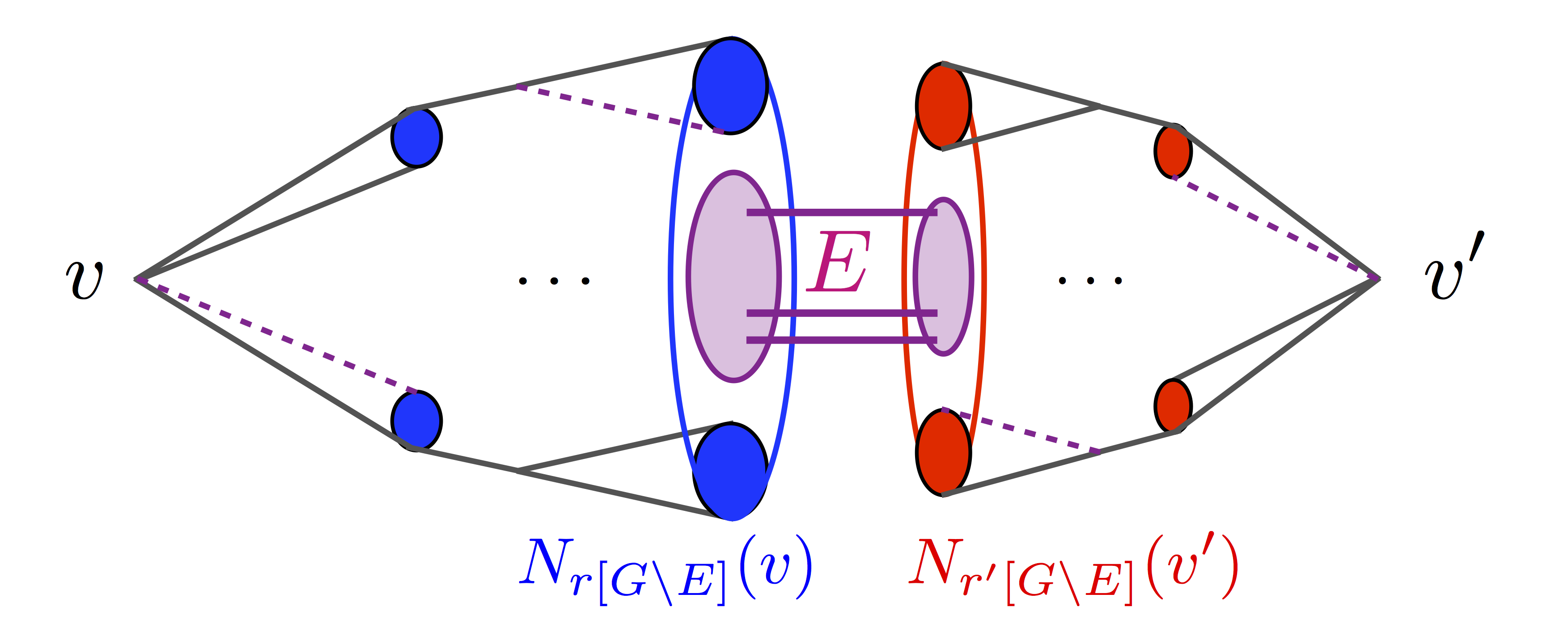
Figure 6.1 provides an illustration of the statistics used. Further, [AS15d] develops an invariant statistics that does not require the knowledge of the model parameters in order to compare the spheres:
Definition 23.
Let be a graph and let be the edge set obtained by sampling each edge with probability (i.e., the graph-split). For two vertices in , define the sign-invariant statistics as
| (6.3) |
The key property is that this statistics with high probability scales as
| (6.4) |
In particular, for odd, will tend to be positive if and are in the same community and negative otherwise, irrespective of the specific values of . That suggests the following agnostic algorithm for partial recovery:
Agnostic-sphere-comparison. Input: an -vertex graph and a parameter . Let be the average degree of the graph:
- 1.
Set and put each of the graph’s edges in with probability .
- 2.
Among distinct vertices such that , pick two of maximal sum-degree, and assign each of these to a different community. Assign each vertex to the community maximizing .
A variant of this algorithm (that applies to the general SBM) is shown in [AS15d] to solve almost exact recovery efficiently under the conditions of Theorem 21. We conclude this section by noting that one can also study more specific almost exact recovery requirements, allowing for a specified number of misclassified vertices . This is investigated in [YP15] when is moderately small (at most logarithmic), with an extension of Theorem 21 that applies to this more general setting. The case where is linear, i.e., a constant fraction of errors, is more challenging and is discussed in the next sections.
6.2 Partial recovery at finite SNR
Recall that partial recovery refers to the case that a fraction of misclassified vertices is constant, whereas the previous section investigates the case that a fraction of misclassified vertices is vanishing.
In the symmetric , the regime for partial recovery takes place when the following notion of SNR is finite:
| (6.5) |
This takes place under two circumstances:
- I.
If are constant, i.e., the constant degree regime,
- II.
If are functions of that diverge such that the numerator and denominator in scale proportionally.
Our main goal is to identify the optimal tradeoff between and the fraction of misclassified vertices, or between and the MMSE or the mutual information of the reconstruction. The latter has particular application to the compression of graphs [Abb16, AAV17]. We first mention some bounds.
Upper bounds on the fraction of incorrectly recovered vertices were demonstrated, among others, in [AS15a, YP14a, CRV15, GMZZ15], taking form when is large. A bound that applies to the general SBM with arbitrary connectivity matrix is also provided in [AS15a]. In [YP14a], a spectral algorithm is shown to reach an upper-bound of for the two-community symmetric case and in a suitable asymptotic sense. An upper bound of the form —again for a spectral algorithm—was obtained earlier in [CRV15]. Further, [GMZZ15] also establishes minimax optimal rate of in the case of large and for certain types of SBMs, further handling a growing number of communities (to the expense of looser bounds).
The optimal fraction of nodes that can be recovered was obtained in [MNS13] for two symmetric communities when the degrees are constant but the SNR is sufficiently large, connecting to the broadcasting problem on tree problem [EKPS00]. This result is further discussed below. It remains open to establish such a result at arbitrary finite SNR.
We next describe a result that gives the optimal tradeoff between the SNR and the MMSE (or the mutual information) for the two-symmetric SBM in the second regime, where SNR is finite (and arbitrary) but where degrees diverge. After that, we discuss results for constant degrees but large enough SNR.
6.3 Mutual Information-SNR tradeoff
In this section, we study the finite SNR regime with diverging degrees and show that the SBM is essentially equivalent to a spiked Wigner model (i.e., a low-rank matrix perturbed by a Wigner random matrix), where the spiked signal has a block structure (rather than a sparse structure as in sparse PCA [BR13, DM14]). To compare the two models, we use the mutual information.
In this section we use in lieu of , i.e., the inner- and outer-cluster probabilities. For , the mutual information of the SBM is , where
and denotes the entropy. We next introduce the normalized MMSE of the SBM:
| (6.6) | ||||
| (6.7) |
where denotes the Frobenius norm.
To state the result that provides a single-letter characterization of the per-vertex MMSE (or mutual information), we need to introduce the effective Gaussian scalar channel. Namely, define the Gaussian channel
| (6.8) |
where independent of . We denote by and the corresponding minimum mean square error and mutual information:
| (6.9) | ||||
| (6.10) |
Note that these quantities can be written explicitly as Gaussian integrals of elementary functions:
| (6.11) | ||||
| (6.12) |
We are now in position to state the result.
Theorem 22.
Let and define11 1 Note that this is asymptotically the same notion of SNR as defined earlier when vanish. Assume that, as , and . Then,
| (6.15) | ||||
| (6.16) |
Further, this implies for (i.e., weak recovery unsolvable) and for (i.e., weak recovery solvable).
Corollary 4.
A few remarks about the previous theorem and corollary:
- •
Theorem 22 shows that the normalized MMSE (or mutual information) is non-trivial if and only if . This extends the results on weak recovery [Mas14, MNS15] discussed in Section 7.2 for the regime of finite SNR with diverging degrees, completing weak recovery in the SSBM with two communities and any choice of parameters;
- •
- •
In [MX15], tight expressions similar to those obtained in Theorem 22 for the MMSE are obtained for the optimal expected agreement with additional scaling requirements. Namely, it is shown that for with and , the least fraction of misclassified vertices is in expectation given by where is the unique fixed point of the equation , is normal distributed, and is the Q-function for the normal distribution. Similar expressions were also derived in [ZMN16] for the overlap metric, and [LKZ15] for the MMSE.
- •
Note that Theorem 22 requires merely diverging degrees (arbitrarily slowly), in contrast to general results from random matrix theory such as [BBAP05] that would require poly-logarithmic degrees to extract communities from the spiked Wigner model point of view. We refer to [PWBM16b, PWB16, BMV+] and references therein for generalizations of the spiked Wigner model discussed here with more general input signals.

6.4 Proof technique and connections to spiked Wigner models
Theorem 22 gives an exact expression for the normalized MMSE and mutual information in terms of an effective Gaussian noise channel. The Gaussian distribution emerges due to a universality result established in the proof: in the regime of the theorem, the SBM model is equivalent to a spiked Wigner model given by
where is a Wigner random matrix (i.e., symmetric with i.i.d. Normal entries), and where we recall that corresponds to the limit of .
The formal statement of the equivalence is as follows:
Theorem 23 (Equivalence of SBM and a spiked Wigner model).
Let be the mutual information of with and , and be the mutual information for spiked Wigner model . Then, there is a constant independent of such that
| (6.20) |
To obtain the limiting expression for the normalized mutual information in Theorem 22, first notice that for ,
Next, (i) use the fundamental theorem of calculus to express these boundary conditions as an integral of the derivative of the mutual information, (ii) use the I-MMSE identity [GSV05] to express this derivative in terms of the MMSE, (iii) upper-bound the MMSE using a specific estimator obtained from the AMP algorithm [DMM09] (or any algorithm performing optimally in this regime), (iv) evaluate the asymptotic performance of the AMP estimate using the density evolution technique [BM11, DM14], and (v) note that the obtained bound matches the original value of in the limit of tending to infinty:
| (6.21) | ||||
| (6.22) | ||||
| (6.23) | ||||
| (6.24) | ||||
| (6.25) |
This implies that (iii) is in fact an equality asymptotically, and using monotonicity and continuity properties of the integrand, the identity must hold for all SNRs as stated in the theorem. The only caveat not discussed here is the fact that AMP needs an initialization that is not fully symmetric to converge to the right solution, which causes the insertion in the proof of a noisy genie on the true labels at the channel output to break the symmetry for AMP. The genie is then removed by taking noise parameters that are arbitrarily large.
6.5 Partial recovery for constant degrees
Obtaining the expression for the optimal agreement at finite and arbitrary SNR when the degrees are constant remains an open problem (see also Sections 6.1 and 10). The problem is settled for high enough SNR in [MNS13], with the following expression relying on reconstruction error for the broadcasting on trees problem.
Define the optimal agreement fraction as
| (6.26) |
Note that the above expression takes into account the symmetry of the problem and can also been interpreted both as a normalized agreement and probability. Let . Define now the counterpart for the broadcasting problem on tree: Back to the notation of Section 5.1, define as the Galton-Watson tree with Poisson offspring, flip probability and depth , and define the optimal inference probability of the root as
| (6.27) |
The reduction from [MNS15] discussed in Section 5.1 allows to deduce that , and this is shown to be an equality for large enough SNR:
Theorem 24.
[MNS13] There exists large enough such that if then , and this normalized agreement is efficiently achievable.
The theorem in [MNS13] has a weaker requirement of , but later developments on weak recovery imply for free the version stated above. Note that gives an implicit expression for the optimal fraction, though it admits a variational representation due to [MM06]. The efficient algorithm is a variant of belief propagation.
In [DKMZ11], it is conjectured that BP gives the optimal agreement at all SNR. However, as discussed in Section 3.4, BP is hard to analyze in the context of loopy graphs with a random initialization. Another strategy is to proceed with a two-round procedure, which is used to establish the above results in [MNS13] for two communities. The idea is to use a simpler algorithm to obtain a non-trivial reconstruction when , see Section 7.2, and then to improve the accuracy using full BP at shorter depth. To show that the accuracy achieved is optimal, one also has to show that a noisy version of the reconstruction on tree problem [JM04], where leaves do not have exact labels but noisy labels, leads to the same probability of error at the root. This is expected to take place for two communities at all SNR above the KS threshold, and it was shown in [MNS13] for the case of large enough SNR. This type of claim is not expected to hold for general . For more than two communities, one needs to first convert the output of the algorithm discussed in Section 5.3.1, which gives two sets that correlated with their communities, into a nontrivial assignment of a belief to each vertex; this is discussed in [AS17]. Then one can use these beliefs as starting probabilities for a belief propagation algorithm of depth , which now runs on a tree-like graph.
Chapter 7 The general SBM
In this section we discuss results for the general SBM, where communities can take arbitrary relative sizes and where connectivity rates among communities are arbitrary.
7.1 Exact recovery and CH-divergence
We provide the fundamental limit for exact recovery in the general SBM, in the regime of the phase transition where scales like for a matrix with positive entries.
Theorem 25.
[AS15a] Exact recovery in is solvable and efficiently so if
and is not solvable if , where is defined by
| (7.1) |
Remark 5.
Regarding the behavior at the threshold: If all the entries of are non-zero, then exact recovery is solvable (and efficiently so) if and only if . In general, exact recovery is solvable at the threshold, i.e., when , if and only if any two columns of have a component that is non-zero and different in both columns.
Remark 6.
In the symmetric case , the CH-divergence is maximized at the value of , and it reduces in this case to the Hellinger divergence between any two columns of ; the theorem’s inequality becomes
matching the expression obtained in Theorem 3 for two symmetric communities.
We now discuss some properties of the functional governing the fundamental limit for exact recovery in Theorem 25. For , let
| (7.2) |
and note that . Since the function satisfies
- •
- •
is convex on ,
the functional is a so-called -divergence [Csi63], like the KL-divergence (), the Hellinger divergence, or the Chernoff divergence. Such functionals have a list of common properties described in [Csi63]. For example, if two distributions are perturbed by additive noise (i.e., convolving with a distribution), then the divergence always increases, or if some of the elements of the distributions’ support are merged, then the divergence always decreases. Each of these properties can be interpreted in terms of community detection (e.g., it is easier to recovery merged communities, etc.). Since collapses to the Hellinger divergence when and since it matches the Chernoff divergence for probability measures, we call (and the Chernoff-Hellinger (CH) divergence in [AS15a].
Theorem 25 thus gives a new operational meaning to an -divergence, showing that the fundamental limit for data clustering in SBMs is governed by the CH-divergence, similarly to the fundamental limit for data transmission in DMCs being governed by the KL-divergence. If the columns of are “different” enough, where difference is measured in CH-divergence, then one can separate the communities. This is analogous to the channel coding theorem that says that when the output’s distributions are “different” enough, where difference is measured in KL-divergence, then one can separate the codewords.
7.1.1 Converse
Let . Recall that to solve exact recovery, we need to find the partition of the vertices, but not necessarily the actual labels. Equivalently, the goal is to find the community partition as defined in Section 2. Recall also that the optimal estimator (see Section 4) is the MAP estimator that maximizes the posterior distribution
| (7.3) |
or equivalently
| (7.4) |
and any such maximizer can be chosen arbitrarily. If MAP fails in solving exact recovery, no other algorithm can succeed.
We proceed similarly to the symmetric case to obtain the impossibility part of Theorem 25, i.e., we reduce the problem to a genie hypothesis test for recovering a single vertex given the other vertices. However, we now work in the Bernoulli community prior model, for slight conveniences.
Imagine that in addition to observing , a genie provides the observation of . Define now for and
| (7.5) |
where ties can be broken arbitrarily if they occur (we assume that an error is declared in case of ties to simplify the analysis). If we fail at recovering a single component when all others are revealed, we must fail at solving exact recovery all at once, thus
| (7.6) |
This lower bound may appear to be loose at first, as recovering the entire communities from the graph seems much more difficult than classifying each vertex by having all others revealed (we call the latter component-MAP). As shown for the two symmetric case in Section 4, the obtained bound is, however, tight.
Let . If the events were independent, we could write and if , this would drive , and thus , to 1. The events are not independent, but their dependencies are weak enough that previous reasoning still applies, and is driven to 1 when . In Section 4, we used the second moment method to obtain this statement, showing that the events are asymptotically independent, which we also pursue below. In [AS15a], a variant of this method is used to obtain the conclusion.
Recall that for the second moment method, one defines
which counts the number of components where component-MAP fails. Note that the right hand side of (7.6) corresponds to as desired. Our goal is to show that stays strictly below 1 in the limit, or equivalently, stays strictly below 2 in the limit. In fact, the latter tends to in the converse of Theorem 25.
Note that where are binary random variables with for all . Hence, tends to 1 if
| (7.7) |
which takes place if and .
The location of the threshold is then dictated by requirement that diverges, and this where the CH-divergence threshold emerges from a moderate deviation analysis. We next summarize what we obtained with the above reasoning, and then specialized to the regime of Theorem 25.
Theorem 26.
Let , , . If the events and are asymptotically independent, then exact recovery is not solvable if
| (7.8) |
The next lemma gives the behavior of in the logarithmic degree regime.
Lemma 14.
[AS15a] Consider the hypothesis test where has prior probability for , and where observable is distributed under hypothesis . This is called degree-profiling in [AS15a], and is illustrated in Figure 7.1. Then the probability of error of MAP decoding for this test satisfies where
and for a symmetric ,
| (7.9) |
where .
Corollary 5.
Let where is constant and . Then
| (7.10) |
A robust extension of this Lemma is proved in [AS15a] that allows for a slight perturbation of the binomial distributions.
7.1.2 Achievability
Two-round algorithms have proved to be powerful in the context of exact recovery. The general idea consists in using a first algorithm to obtain a good but not necessarily exact clustering, solving a joint assignment of all vertices, and then to switch to a local algorithm that “cleans up” the good clustering into an exact one by reclassifying each vertex. This approach has a few advantages:
- •
If the clustering of the first round is accurate enough, the second round becomes approximately the genie-aided hypothesis test discussed in previous section, and the approach is built in to achieve the threshold;
- •
if the clustering of the first round is efficient, then the overall method is efficient since the second round only performs computations for each single node separately and has thus linear complexity.
Some difficulties need to be overome for this program to be carried out:
- •
One needs to obtain a good clustering in the first round, which is typically non-trivial;
- •
One needs to be able to analyze the probability of success of the second round, as the graph is no longer independent of the obtained clusters.
To resolve the latter point, we rely in [ABH16] on the technique which we call “graph-splitting” and which takes again advantage of the sparsity of the graph.
Definition 24 (Graph-splitting).
Let be an -vertex graph and . The graph-splitting of with split-probability produces two random graphs on the same vertex set as . The graph is obtained by sampling each edge of independently with probability , and (i.e., contains the edges from that have not been subsampled in ).
Graph splitting is convenient in part due to the following fact.
Lemma 15.
Let , be a graph splitting of with split-probability , and with independent of . Let be valued in such that . For any , ,
| (7.11) |
where is the degree profile of vertex , i.e., the -dimensional vector counting the number of neighbors of vertex in each community using the clustered graph .
The meaning of this lemma is as follows. We can consider and to be approximately independent, and export the output of an algorithm run on to the graph without worrying about dependencies to proceed with component-MAP. Further, if is to chosen as where , then is distributed as and remains approximately as . This means that from our original SBM graph, we produce essentially ‘for free’ a preliminary graph with expected degrees that can be used to get a preliminary clustering, and we can then improve that clustering on the graph which has still logarithmic expected degree.
Our goal is to obtain on a clustering that is almost exact, i.e., with only a vanishing fraction of misclassified vertices. If this can be achieved for some that is , then a robust version of the genie-aided hypothesis test described in Section 7.1.1 can be run to re-classify each node successfully when . Luckily, as we shall see in Section 6.1, almost exact recovery can be solved with the mere requirement that (i.e., diverges). In particular, setting does the job. We next describe more formally the previous reasoning.
Theorem 27.
If almost exact recovery is solvable in , then exact recovery is solvable in if
| (7.12) |
To see this, let , and be a graph splitting of with split-probability . Let with independent of (note that the same appears twice). Let be valued in such that ; note that such an exists from the theorem’s hypothesis. Since with high probability, are functions of and using a union bound, we have
| (7.13) | ||||
| (7.14) | ||||
| (7.15) | ||||
| (7.16) |
We next replace by . Note that has already the same marginal as , the only issue is that is not independent from since the two graphs are disjoint, and since is derived from , some dependencies are carried along with . However, and are ‘essentially independent’ as stated in Lemma 15, because the probability that samples an edge that is already present in is , and the expected degrees in each graph is . This takes us to
| (7.17) | ||||
| (7.18) |
We can now replace with to the expense that we may blow up this the probability by a factor since , again using the fact that expected degrees are logarithmic. Thus we have
| (7.19) | ||||
| (7.20) |
and the conditioning on can now be removed due to independence, so that
| (7.21) |
The last step consists in closing the loop and replacing by , since , which uses the same type of argument as for the replacement of by , with a blow up that is at most . As a result,
| (7.22) |
and if
| (7.23) |
for , then is vanishing as stated in the theorem.
Therefore, in view of Theorem 27, the achievability part of Theorem 25 reduces to the following result.
Theorem 28.
[AS15a] Almost exact recovery is efficiently solvable in .
This follows from Theorem 31 discussed below, based on the Sphere-comparison algorithm discussed in Section 6.
In conclusion, in the regime of Theorem 25, exact recovery can be shown by using graph-splitting and combining almost exact recovery with degrees that grow sub-logarithmically and an additional clean-up phase. The behavior of the component-MAP error (i.e., the probability of misclassifying a single node when others have been revealed) pings down the behavior of the threshold: if this probability is , exact recovery is not possible, and if it is , exact recovery is possible. Decoding for the latter is then resolved by obtaining the exponent of the component-MAP error, which brings in the CH-divergence.
Local to global amplification. The previous two sections give a lower bound and an upper bound on the probability that MAP fails at recovering the entire clusters, in terms of the probability that MAP fails at recovering a single vertex when others are revealed. Denoting by and these two probabilities of error, we essentially11 1 The upper bound discussed in Section 7.1.2 gives , but the analysis can be tighten to yield a factor instead of . have
| (7.24) |
This implies that has a threshold phenomena as varies:
| (7.25) |
Moreover, deriving this relies mainly on the regime of the model, rather than the specific structure of the SBM. In particular, it mainly relies on the exchangeability of the model (i.e., vertex labels have no relevance) and the fact that the vertex degrees do not grow rapidly. This suggests that this ‘local to global’ phenomenon takes place in a more general class of models. The expression of the threshold for exact recovery in as a function of the parameters is instead specific to the model, and relies on the CH-divergence in the case of the SBM, but the moderate/large deviation analysis of for other models may reveal a different functional or -divergence.
The local to global approach also has an important implication at the computational level. The achievability proof described in the previous section directly gives an algorithm: use graph-splitting to produce two graphs; solve almost exact recovery on the first graph and locally improve the obtained clusters with the second graph. Since the second round is efficient by construction (it corresponds to parallel local computations), it is sufficient to solve almost exact recovery efficiently (in the regime of diverging degrees) to obtain for free an efficient algorithm for exact recovery down to the threshold. Thus this gives a computational reduction. In fact, the process can be iterated to further reduce almost exact recovery to a weaker recovery requirements, until a ‘bottle-neck’ recovery problem is attained.
7.2 Weak recovery and generalized KS threshold
We recall the conjecture stated in [DKMZ11]:
Conjecture 1.
[DKMZ11, MNS15] Let be drawn from , i.e., the symmetric SBM with communities, probability inside the communities and across. Define . Then,
- (i)
For any , it is possible to solve weak recovery efficiently if and only if (the Kesten-Stigum (KS) threshold);
- (ii)
If22 2 The conjecture states that is necessary when imposing the constraint that , but is enough in general. , it is possible to solve weak recovery information-theoretically (i.e., not necessarily in polynomial time in ) for some strictly below 1.33 3 [DKMZ11] made in fact a more precise conjecture, stating that below the KS threshold, there is a second transition for information-theoretic methods when , whereas there is a single threshold (for both efficient or non-efficient algorithms) when .
It was also shown in [BLM15] that for SBMs with communities that are balanced and for parameters that satisfy a certain asymmetry condition, i.e., the requirement that is a simple eigenvalue in Theorem 5 of [BLM15], the KS threshold can be achieved efficiently. The conditions of [BLM15] do not cover Conjecture 1 for . In [AS15c, AS17], the two positive parts of the above conjecture are proved, with an extended result applying to the general SBM. We next discuss these various results.
Given parameters and in the general model , let be the diagonal matrix such that for each . Also, let be the distinct eigenvalues of in order of nonincreasing magnitude.
Definition 25.
Define the signal-to-noise ratio of by
In the community symmetric case where vertices in the same community are connected with probability and vertices in different communities are connected with probability , we have , which matches the quantity in Conjecture 1 and in all previous sections concerned with two communities.
Theorem 29.
[BLM15] Let such that and such that has an eigenvector with corresponding eigenvalue in of single multiplicity. If , then weak recovery is efficiently solvable.
Theorem 30 implies the achievability part of Conjecture 1 part (i).
The algorithm used in [BLM15] is a spectral algorithm using the second eigenvector of the NB matrix discussed in Section 5.3.1. The algorithm used in [AS17] is an approximate acyclic belief propagation (ABP) algorithm, which corresponds to a power iteration method to extract the second eigenvector of the -NB matrix.
Remark 7.
Also note that it is important to use the notion of weak recovery defined in Section 4, where the agreement is normalized by the sizes of the communities. Without this normalization, using naively “beating a random guess” or the definition of [DKMZ11], the conjecture that weak recovery is efficiently solvable if and only if is not true in general; a counter-example is given in [AS17] where the max-detection criteria of [DKMZ11] is not solvable when .
We conjecture that Theorem 30 is tight, i.e., if , then efficient weak recovery is not solvable. However, establishing formally such a converse argument seems out of reach at the moment: as we shall see in the next section, except for a few possible cases with low values of (e.g., symmetric SBMs with ), it is possible to detect information-theoretically when , and thus one cannot get a converse for efficient algorithms by considering all algorithms.
7.3 Partial recovery
The Sphere-comparison algorithm discussed in Section 6.1 gives the following result:
Theorem 31.
[AS15b] For any , and with no two rows equal, there exist such that for all sufficiently large , Sphere-comparison detects communities in SBM with accuracy and complexity .
Chapter 8 The information-computation gap
In this section we discuss SBM regimes where weak recovery can be solved information-theoretically. As stated in Conjecture 1 and proved in Theorem 30, the information-computation gap—defined as the gap between the KS and IT thresholds—takes place when the number of communities is larger than 4. We provide an information-theoretic (IT) bound for that confirms this, showing further that the gap can grow fast with the number of communities.
The information-theoretic bound described below is obtained by using a non-efficient algorithm that samples uniformly at random a clustering that is typical, i.e., that has the right proportions of edges inside and across the clusters. We describe below how this gives a tight expression in various regimes. Note that to capture the exact information-theoretic threshold in all regimes, one would have to rely on tighter estimates on the posterior distribution of the clusters given the graph. A possibility is to estimate the limit of the normalized mutual information between the clusters and the graph, i.e., , as done in [DAM15] for the regime of finite SNR with diverging degrees11 1 Similar results were also obtained recently in a more general context in [CLM16, LM].—see Section 6.3. Recent results also obtained the expression for the finite degree regime in the disassortative case [CKPZ16]. Another possibility is to estimate the limiting total variation or KL-divergence between the graph distribution in the SBM vs. Erdős-Rényi model of matching expected degree. The limiting total variation is positive if and only if an hypothesis test can distinguish between the two models with a chance better than half. The easy implication of this is that if the total variation is vanishing, the weak recovery is not solvable (otherwise we would detect virtual clusters in the Erdős-Rényi model). This used in [BM16] to obtain a lower-bound on the information-theoretic threshold, using a contiguity argument, see further details at the end of this section.
8.1 Crossing KS: typicality
To obtain our information-theoretic upper-bound, we rely on the following sampling algorithm:
Typicality Sampling Algorithm. Given an -vertex graph and , the algorithm draws uniformly at random in
where the above assumes that ; flip the above two inequalities in the case .
We present below a bound that we claim is tight at the extremal regimes of and (see discussions below). Note that for , is simply a patching of disjoint Erdős-Rényi random graphs, and thus the information-theoretic threshold corresponds to the giant component threshold, i.e., , achieved by separating the giants. This breaks down for positive, but we expect that the bound derived below remains tight in the scaling of small . For , the problem corresponds to planted coloring, which is already challenging [AK97]. The bound obtained below gives that, in this case, weak recovery is information-theoretically solvable if , . This scaling is further shown to be tight in [BM16], which also provides a simple upper-bound that scales as for . Overall, the bound below shows that the KS threshold gives a much more restrictive regime than what is possible information-theoretically, as the latter reads for .
Theorem 32.
Let , assume , and let be the unique solution in of , i.e., . The Typicality Sampling Algorithm solves weak recovery22 2 Setting small enough gives the existence of for weak recovery. communities in if
| (8.1) | ||||
| (8.2) | ||||
| (8.3) |
This bound strictly improves on the KS threshold for . See [AS17] for a numerical example.
Corollary 6.
Conjecture 1 part (ii) holds.
Note that (8.3) simplifies to
| (8.4) |
and since when (which is needed for the presence of the giant), weak recovery is already solvable in if
| (8.5) |
The above bound corresponds to the regime where there is no bad clustering that is typical with high probability. The analog of this bound in the unbalanced case already provides examples to crossing KS for two communities, such as for and . However, the above bound is not tight in the extreme regime of , since it reads as opposed to , and it only crosses the KS threshold at . Before explaining how to obtain tight interpolations, we provide further insight on the bound of Theorem 32.
Defining as the unique solution of
| (8.6) | ||||
| (8.7) |
and simplifying the bound in Theorem 32 gives the following.
Corollary 7.
Weak recovery is solvable
| (8.8) | ||||
| (8.9) |
Remark 8.
Note that (8.9) approaches the optimal bound given by the presence of the giant at , and we further conjecture that gives the correct first order approximation of the information-theoretic bound for small .
Remark 9.
Note that the -colorability threshold for Erdős-Rényi graphs grows as [AN05]. This may be used to obtain an information-theoretic bound, which would however be looser than the one obtained above.
It is possible to see that this gives also the correct scaling in for , i.e., that for , , weak recovery is information-theoretically impossible. To see this, consider , , and assume that we know the communities of all vertices more than edges away from . For each vertex edges away from , there will be approximately communities that it has no neighbors in. Then vertices edges away from have approximately neighbors that are potentially in each community, with approximately fewer neighbors suspected of being in its community than in the average other community. At that point, the noise has mostly drowned out the signal and our confidence that we know anything about the vertices’ communities continues to degrade with each successive step towards .
A different approach is developed in [BM16] to prove that the scaling in is in fact optimal, obtaining both upper and lower bounds on the information-theoretic threshold that match in the regime of large when . In terms of the expected degree, the threshold reads as follows.
Theorem 33.
The upper-bound in [BM16] corresponds essentially to (8.5), the regime in which the first moment bound is vanishing. The lower-bound is based on a contiguity argument and second moment estimates from [AN05]. The idea is to compare the distribution of graphs drawn from the SBM, i.e.,
| (8.10) |
with the distribution of graphs drawn from the Erdős-Rényi model with matching expected degree, call it . If one can show that
| (8.11) |
then upon observing a graph drawn from either of the two models, say with probability half for each, it is impossible to decide from which ensemble the graph is drawn with high probability. Thus it is not possible to solve weak recovery (otherwise one would detect clusters in the Erdős-Rényi model). A sufficient condition to imply (8.11) is to show that , i.e., for any sequence of event such that , it must be that . In particular, and are called contiguous if and , but only the first of these conditions is needed here. Further, this is implied from Cauchy-Schwarz if the ratio function
has a bounded second moment, i.e.,
8.2 Nature of the gap
The nature of such gap phenomena can be seen from different perspectives. One interpretation comes from the behavior of belief propagation. See also [Moo17] for further discussions.
Above the Kesten-Stigum threshold, the uniform fixed point is unstable and BP does not get attracted to it and reaches a non-trivial solution on most initializations. In particular, the ABP algorithm discussed in Section 5.3.1, which starts with a random initialization with order vertices towards the true partition (due to the Central Limit Theorem), is enough to make linearized BP reach a non-trivial fixed point. Below the information-theoretic threshold, the non-trivial fixed points are no longer present, and BP settles in a solution that represents a noisy clustering, i.e., one that would also take place in the Erős-Rényi model due to the noise fluctuations in the model. In the gap region, non-trivial fixed points are still present, but the trivial fixed points are locally stable and attract most initializations. One could try multiple initializations until a non-trivial fixed point is reached, using for example the graph-splitting technique discussed in Section 5.2.2 to test such solutions. However, it is believed that an exponential number of initializations is needed to reach a good solution.
This connects to the “energy landscape” of the possible clusterings: in this gap region, the non-trivial fixed points have a very small basin of attraction, and they can only attract an exponentially small fraction of initializations. To connect to the results from Section 7.1, the success of the two-round procedure can also be related to the energy landscape, i.e., the objective function of MAP in this case. Above the CH threshold, an almost exact solution having correctly labeled vertices can be converted to an exact solution by the degree-profiling hypothesis test. This is essentially saying that BP at depth 1, i.e., computing the likelihood of a vertex based on its direct neighbors, allows us to reach the global maximum of the likelihood function with such a strong initialization. In other words, the BP view, or more precisely understanding the question of how accurate our initial beliefs need to be in order to amplify these to non-trivial levels based on neighbors at a given depth, is related to the landscape of the objective function.
The gap phenomenon also admits a local manifestation in the context of ABP, having to do with the approximation discussed in Section 5.3.1, where the non-linear terms behave differently from to due to the loss of a diminishing return property. Better understanding such gap phenomena is an active research area.
8.3 Proof technique for crossing KS
We explain in this section how to obtain the bound in Theorem 32. A first problem is to estimate the likelihood that a bad clustering, i.e., one that has an overlap close to with the true clustering, belongs to the typical set. As clusters sampled from the TS algorithm are balanced, a bad clustering must split each cluster roughly into balanced subgroups that belong to each community, see Figure 8.1. Thus it is unlikely to keep the right proportions of edges inside and across the clusters, but depending on the exponent of this rare event, and since there are exponentially many bad clusterings, there may exist one bad clustering that looks typical.

As illustrated in Figure 8.1, the number of edges that are contained in the clusters of a bad clustering is roughly distributed as the sum of two Binomial random variables,
where we use to emphasize that this is an approximation that ignores the fact that the clustering is not perfect bad and perfectly balanced. Note that the expectation of the above distribution is . In contrast, the true clustering would have a distribution given by , which would give an expectation of . In turn, the number of edges that are crossing the clusters of a bad clustering is roughly distributed as
which has an expectation of . In contrast, the true clustering would have the above replaced by , and an expectation of .
Thus, we need to estimate the rare event that the Binomial sum deviates from its expectation. While there is a large list of bounds on Binomial tail events, the number of trials here is quadratic in and the success bias decays linearly in , which require particular care to ensure tight bounds. We derive these in [AS15c], obtaining that behaves as
when are arbitrarily small, where . One can then use the fact that with high probability, since the planted clustering is typical with high probability, and using a union bound and the fact that there are at most bad clusterings:
| (8.12) | ||||
| (8.13) | ||||
Checking when the above upper-bound vanishes already gives a regime that crosses the KS threshold when for symmetric communities, when for asymmetric communities (deriving the version of the bound for asymmetric communities), and scales properly in when . However, it does not interpolate the correct behavior of the information-theoretic bound in the extreme regime of and does not cross at . In fact, for , the union bound requires to imply no bad typical clustering with high probability, whereas as soon as , an algorithm that simply separates the two giants in and assigns communities uniformly at random for the other vertices solves weak recovery. Thus when , the union bound is loose. To remediate this, we next take into account the topology of the SBM graph to tighten our bound on .
Since the algorithm samples a typical clustering, we only need the number of bad and typical clusterings to be small compared to the total number of typical clusterings, in expectation. Namely, we can get a tighter bound on the probability of error of the TS algorithm by obtaining a tighter bound on the typical set size than simply 1, i.e., estimating (8.12) without relying on the loose bound from (8.13). We proceed here with three levels of refinements to bound the typical set size. In each level, we construct a random labelling of the vertices that remains typical, and then use entropic estimates to count the number of such typical labellings.
First we exploit the large fraction of nodes that are in tree-like components outside of the giant, and the labels are distributed on such trees as in the broadcasting on trees problem 5.1. Specifically, for a uniformly drawn root node , each edge in the tree acts as a -ary symmetric channel. Thus, labelling the nodes in the trees according to the above distribution and freezing the giant to the correct labels leads to a typical clustering with high probability. The resulting bound matches the giant component bound at , but is unlikely to scale properly for small . To improve on this, we next take into account the vertices in the giant that belong to planted trees, and follow the same program as above, except that the root node (in the giant) is now frozen to the correct label rather than being uniformly drawn. This gives a bound that we claim is tight at the first order approximation when is small. Finally, we also take into account vertices that are not saturated, i.e., whose neighbors do not cover all communities and who can thus be swapped without affecting typicality. The final bound allows to cross at .

Chapter 9 Other block models
There are various extensions of the basic SBM discussed in previous section. The variations increase yearly, and we mention here a few basic variants:
- •
- •
- •
Overlapping SBMs: allowing for the communities to overlap, such as in the mixed-membership SBM [ABFX08], where each vertex has a profile of community memberships or a continuous label—see also [For10, NP15, BKN11, Pei15, PDFV05, GB13, AS15a]; also [Abb17] for reductions to non-overlapping community models in some cases and recent results that sharp for MMSBM in [HS17];
- •
Definition 26 (Geometric block models).
We define here two geometric block models with two communities, the sphere-GBM and the mixture-GBM. For each model, has i.i.d. Bernoulli components, which represents the abstract community labels for each vertex. We next add a geometric label for each vertex, and draw the graph depending on both the abstract and geometric labels:
- •
In the sphere-GBM, has i.i.d. components drawn uniformly at random on a sphere of dimension ; the graph is drawn with edges independent conditionally on , such that for ,
(9.1) and . One can have a variant with a special symbol that indicates if .
- •
In the mixture-GBM, has independent components conditionally on with drawn from if and from if (two isotropic Gaussians in dimension at distance ); the graph is drawn with edges independent conditionally on , such that for ,
(9.2) and .
In dimension , we want to be at least of order with a large enough constant in order for the graphs to have giant components, and with a large enough constant for connectivity.
Previous models have a much larger number of short loops than the SBM does, which captures a feature of various real world graphs having transitive attributes (“friends of friends are more likely to be friends”). On the flip side, these models do not have ‘abstract edges’ as in the SBM, which can also occur frequently in applications given the “small-world phenomenon”. This says that real graphs often have relatively low diameter (about 6 in the case of Milgram’s experiment), which does not take place in purely geometric block models. Therefore, a natural candidate is to superpose an SBM and a GBM to form an hybrid block model (HBM), see for example [ABS17b]. The many loops of the GBM can be challenging for some of the algorithms discussed in this monograph, in particular for basic spectral methods and even belief propagation; we discussed in Section 5.3.2 how graph powering provides a more robust alternative in such cases.
Another variant that circumvents the discussions about non-edges is to consider a censored block model (CBM), defined as follows (see [HLM, ABBS14a]).
Definition 27 (Binary symmetric CBM).
Let be a graph and . Let with i.i.d. Bernoulli components. Let be a random vector of dimension taking values in such that
| (9.3) | ||||
| (9.4) |
The case of an Erdős-Rényi graph is discussed in [ABBS14a, ABBS14b, CRV15, SKLZ, CHG14, CG14] and the case of a grid in [AMM+17]. For a random geometric graph on a sphere, it is closely related to the above sphere-GBM. Inserting the symbol simplifies a few aspects compared to SBMs, such as Lemma 12, which is needed in the weak recovery converse of the SBM. In this sense, the CBM is a more convenient model than the SBM from a mathematical viewpoint, while behaving similarly to the SBM (when is an Erdős-Rényi graph of degree and for the two community symmetric case). The CBM can also be viewed as a synchronization model over the binary field, and more general synchronization models have been studied in [PWBM16b, PWBM16a], with a complete description both at the fundamental and algorithmic level (generalizing in particular the results from Section 6.3).
Note all previously mentioned models are different forms of latent variable models. Focusing on the graphical nature, on can also consider the more general inhomogenous random graphs [BJR07], which attach to each vertex a label in a set that is not necessarily finite, and where edges are drawn independently from a given kernel conditionally on these labels. This gives in fact a way to model mixed-membership, and is also related to graphons, which corresponds to the case where each vertex has a continuous label.
It may be worth saying a few words about the theory of graphons and its implications for us. Lovász and co-authors introduced graphons [LS06, BCL+08, Lov12] in the study of large graphs (also related to Szemerédi’s Regularity Lemma [Sze76]), showing that11 1 Initially in dense regimes and more recently for sparse regimes [BCCZ14]. a convergent sequence of graphs admits a limit object, the graphon, that preserves many local and global properties of the sequence. Graphons can be represented by a measurable function , which can be viewed as a continuous extension of the connectivity matrix used throughout this paper. Most relevant to us is that any network model that is invariant under node labelings, such as most models of practical interest, can be described by an edge distribution that is conditionally independent on hidden node labels, via such a measurable map . This gives a de Finetti’s theorem for label-invariant models [Hoo79, Ald81, DJ07], but does not require the topological theory behind it. Thus the theory of graphons may give a broader meaning to the study of block models, which are precisely building blocks to graphons, but for the sole purpose of studying exchangeable network models, inhomogeneous random graphs give enough degrees of freedom.
Further, many problems in machine learning and networks are also concerned with interactions of items that go beyond the pairwise setting. For example, citation or metabolic networks rely on interactions among -tuples of vertices. These can be captured by extending previous models to hypergraphs.22 2 Recent results for community detection in hypergraphs were obtained in [KBG17].
Chapter 10 Concluding remarks and open problems
One may cast the SBM and the previously discussed variants into a comprehensive class of conditional random fields [Laf01] or graphical channels [AM15], where edge labels depend on vertex labels.
Definition 28.
Let and be a hypergraph with . Let and be two finite sets called, respectively, the input and output alphabets, and be a channel from to called the kernel. To each vertex in , assign a vertex-variable in , and to each edge in , assign an edge-variable in . Let denote the edge-variable attached to edge , and denote the node-variables adjacent to . We define a graphical channel with graph and kernel as the channel given by
![[Uncaptioned image]](1703.10146v3/graphical7.png)
Quantities that are key to understanding how much information can be carried in such graphical channels are:
how “rich” is the observation graph and
how “noisy” is the connectivity kernel .
This survey quantifies the tradeoffs between these two quantities in the SBM (which corresponds to a discrete and a specific graph and kernel ), in order to recover the input from the output. It shows that depending on the recovery requirements, different phase transitions take place: For exact recovery, the CH threshold is efficiently achievable for any fixed number of communities. For weak recovery, the KS threshold is efficiently achievable for any fixed number of communities, but it is not necessarily the information-theoretic threshold, leaving a question mark on whether the KS threshold is indeed the fundamental limit for efficient algorithms. We also presented partial results on the optimal tradeoffs between various measures of distortion and the SNR in the partial recovery regime.
In the quest to achieve these thresholds, novel algorithmic ideas emerged, similarly to the quest to achieve the capacity in channel coding, with sphere-comparison, graph-splitting, linearized BP, nonbacktracking operators and graph powering. This program can now be pursued in different directions, refining the models, improving the algorithms and expanding the realm of applications. In particular, similar tradeoffs are expected to take place in other graphical channels, such as ranking, synchronization, topic modelling, collaboration filtering, planted embeddings and more. We list below a series of possible open problems.
- •
Exact recovery for sub-linear communities. The survey gives a comprehensive treatment for exact recovery with linear-size communities, i.e., when the entries of and its dimension do not scale with . If , most of the developed techniques tend to extend. What happens for larger ? In [ABKK15, YC14], some of this is captured by looking at coarse regimes of the parameters. It would be interesting to pursue sub-linear communities in the lens of phase transitions and information-computation gaps.
- •
Partial recovery. What is the fundamental tradeoff between the SNR and the distortion (MMSE, agreement or mutual information) for partial recovery and arbitrary constant degrees? As a preliminary result, one may attempt to show that admits a limit in the constant degree regime. This is proved in [AM15] for two symmetric disassortative communities, but the assortative case remains open. A recent result from [CKPZ16] further gives the expression for the limit in the disassortative case, but the assortative case remains open.
- •
The information-computation gap:
- –
- –
Can we strengthen the evidence that the KS threshold is the computational threshold? In the general sparse SBM, this corresponds to the following conjecture:
Conjecture 2.
Let , be a probability distribution, be a symmetric matrix with nonnegative entries. If , then there is no polynomial time algorithm that can solve weak recovery (using Definition 4) in drawn from .
- •
Learning the general sparse SBM. Under what conditions can we learn the parameters in efficiently or information-theoretically?
- •
Scaling laws: What is the optimal scaling/exponents of the probability of error for the various recovery requirements? How large need the graph be, i.e., what is the scaling in , so that the probability of error in the discussed results11 1 Recent work [YDHD+16] has investigated finite size information-theoretic analysis for weak recovery. is below a given threshold?
- •
Beyond the SBM:
- –
How do previous results and open problems generalize to the extensions of SBMs with labels, degree-corrections, overlaps (see [HS17]), etc. In the related line of work for graphons [CWA12, ACC13, BCS15], are there fundamental limits in learning the model or recovering the vertex parameters up to a given distortion? The approach of [AS15a] and sphere-comparison were generalized to the case of overlapping communities in [BCLS17] with applications to collaborative filtering. Can we establish fundamental limits and algorithms achieving the limits for other unsupervised machine learning problems, such as topic modelling, ranking, Gaussian mixture clustering (see [BMV+]), low-rank matrix recovery (see [DM14] for sparse PCA) or general graphical channels?
- –
How robust are the thresholds to model perturbations or adversaries? It was shown in [MMV, MPW16] that monotone adversaries can interestingly shift the threshold for weak recovery; what is the threshold for such adversarial models or adversaries having a budget of edges to perturb? What are robust algorithms (see also Section 5.3.2)? What are the exact and weak recovery thresholds in geometric block models (see also previous section)?
- –
- •
Semi-supervised extensions: How do the fundamental limits change in a semi-supervised setting,22 2 Partial results and experiments were obtained for a semi-supervised model [ZMZ14]. Another setting with side-information is considered in [CNM04] with metadata available at the network vertices. Effects on the exact recovery threshold have also been recently investigated in [AAV17]. i.e., when some of the vertex labels are revealed, exactly or probabilistically?
- •
Dynamical extensions: In some cases, the network may be dynamical and one may observe different time instances of the network. How does one integrate such dynamics to understand community detection?33 3 Partial results were recently obtained in [GZC+16].
acknowledgements
I am thankful to my collaborators from the main papers discussed in this monograph, in particular, A. Bandeira, Y. Deshpande, J. Fan, A. Montanari, C. Sandon, K. Wang, Y. Zhong. Special thanks to Colin and Kaizheng for their valuable inputs on this monograph. I would like to also thank the many colleagues with whom I had various conservations on the topic over the past years, in particular, C. Bordenave, F. Krzakala, M. Lelarge, L. Massoulié, C. Moore, E. Mossel, Y. Peres, A. Sly, V. Vu, L. Zdeborová, as well as the colleagues, students and anonymous reviewers who contributed to the significant improvements of the drafts. Finally, I would like to thank the Institute for Advanced Study in Princeton for providing an ideal environment to write part of this monograph.
Bibliography
- [AAV17] A. R. Asadi, E. Abbe, and S. Verdú, Compressing data on graphs with clusters, 2017 IEEE International Symposium on Information Theory (ISIT), June 2017, pp. 1583–1587.
- [Abb16] E. Abbe, Graph compression: The effect of clusters, 2016 54th Annual Allerton Conference on Communication, Control, and Computing (Allerton), Sept 2016, pp. 1–8.
- [Abb17] E. Abbe, Community detection and stochastic block models: recent developments, ArXiv:1703.10146 (2017).
- [ABBS14a] E. Abbe, A.S. Bandeira, A. Bracher, and A. Singer, Decoding binary node labels from censored edge measurements: Phase transition and efficient recovery, Network Science and Engineering, IEEE Transactions on 1 (2014), no. 1, 10–22.
- [ABBS14b] , Linear inverse problems on Erdös-Rényi graphs: Information-theoretic limits and efficient recovery, Information Theory (ISIT), 2014 IEEE International Symposium on, June 2014, pp. 1251–1255.
- [ABFX08] E. M. Airoldi, D. M. Blei, S. E. Fienberg, and E. P. Xing, Mixed membership stochastic block models, J. Mach. Learn. Res. 9 (2008), 1981–2014.
- [ABH14] E. Abbe, A. S. Bandeira, and G. Hall, Exact Recovery in the Stochastic Block Model, ArXiv:1405.3267 (2014).
- [ABH16] E. Abbe, A.S. Bandeira, and G. Hall, Exact recovery in the stochastic block model, Information Theory, IEEE Transactions on 62 (2016), no. 1, 471–487.
- [ABKK15] N. Agarwal, A. S. Bandeira, K. Koiliaris, and A. Kolla, Multisection in the Stochastic Block Model using Semidefinite Programming, ArXiv:1507.02323 (2015).
- [ABS17a] E. Abbe, F. Baccelli, and A. Sankararaman, Community Detection on Euclidean Random Graphs, ArXiv:1706.09942 (2017).
- [ABS17b] E. Abbe, E. Boix, and C. Sandon, Graph powering and spectral gap extraction, Manuscript. Results partly presented at the Simons Institute and partly available in E. Boix PACM Thesis, Princeton University (2017).
- [ACC13] E. Airoldi, T. Costa, and S. Chan, Stochastic blockmodel approximation of a graphon: Theory and consistent estimation, arXiv:1311.1731 (2013).
- [AFWZ17] E. Abbe, J. Fan, K. Wang, and Y. Zhong, Entrywise Eigenvector Analysis of Random Matrices with Low Expected Rank, ArXiv:1709.09565 (2017).
- [AG05] L. Adamic and N. Glance, The political blogosphere and the 2004 U.S. election: Divided they blog, Proceedings of the 3rd International Workshop on Link Discovery (New York, NY, USA), LinkKDD ’05, 2005, pp. 36–43.
- [AK97] Noga Alon and Nabil Kahale, A spectral technique for coloring random 3-colorable graphs, SIAM Journal on Computing 26 (1997), no. 6, 1733–1748.
- [AL14] A. Amini and E. Levina, On semidefinite relaxations for the block model, arXiv:1406.5647 (2014).
- [Ald81] David J. Aldous, Representations for partially exchangeable arrays of random variables, Journal of Multivariate Analysis 11 (1981), no. 4, 581 – 598.
- [AM15] E. Abbe and A. Montanari, Conditional random fields, planted constraint satisfaction, and entropy concentration, Theory of Computing 11 (2015), no. 17, 413–443.
- [AMM+17] E. Abbe, L. Massoulié, A. Montanari, A. Sly, and N. Srivastava, Group Synchronization on Grids, ArXiv:1706.08561 (2017).
- [AN05] Dimitris Achlioptas and Assaf Naor, The two possible values of the chromatic number of a random graph, Annals of Mathematics 162 (2005), no. 3, 1335–1351.
- [ANP05] D. Achlioptas, A. Naor, and Y. Peres, Rigorous Location of Phase Transitions in Hard Optimization Problems, Nature 435 (2005), 759–764.
- [AS15a] E. Abbe and C. Sandon, Community detection in general stochastic block models: Fundamental limits and efficient algorithms for recovery, IEEE 56th Annual Symposium on Foundations of Computer Science, FOCS 2015, Berkeley, CA, USA, 17-20 October, 2015, 2015, pp. 670–688.
- [AS15b] , Community detection in general stochastic block models: fundamental limits and efficient recovery algorithms, arXiv:1503.00609. (2015).
- [AS15c] E. Abbe and C. Sandon, Detection in the stochastic block model with multiple clusters: proof of the achievability conjectures, acyclic BP, and the information-computation gap, ArXiv e-prints 1512.09080 (2015).
- [AS15d] E. Abbe and C. Sandon, Recovering communities in the general stochastic block model without knowing the parameters, Advances in Neural Information Processing Systems (NIPS) 28 (C. Cortes, N.D. Lawrence, D.D. Lee, M. Sugiyama, and R. Garnett, eds.), Curran Associates, Inc., 2015, pp. 676–684.
- [AS16] Emmanuel Abbe and Colin Sandon, Achieving the KS threshold in the general stochastic block model with linearized acyclic belief propagation, Advances in Neural Information Processing Systems 29 (D. D. Lee, M. Sugiyama, U. V. Luxburg, I. Guyon, and R. Garnett, eds.), Curran Associates, Inc., 2016, pp. 1334–1342.
- [AS17] Emmanuel Abbe and Colin Sandon, Proof of the achievability conjectures for the general stochastic block model, Communications on Pure and Applied Mathematics 71 (2017), no. 7, 1334–1406.
- [Ban15] A. S. Bandeira, Random laplacian matrices and convex relaxations, arXiv:1504.03987 (2015).
- [BB14] S. Bhattacharyya and P. J. Bickel, Community Detection in Networks using Graph Distance, ArXiv:1401.3915 (2014).
- [BBAP05] Jinho Baik, Gérard Ben Arous, and Sandrine Péché, Phase transition of the largest eigenvalue for nonnull complex sample covariance matrices, Ann. Probab. 33 (2005), no. 5, 1643–1697.
- [BBEKY13] Derek Bean, Peter J Bickel, Noureddine El Karoui, and Bin Yu, Optimal M-estimation in high-dimensional regression, Proceedings of the National Academy of Sciences 110 (2013), no. 36, 14563–14568.
- [BC09] Peter J. Bickel and Aiyou Chen, A nonparametric view of network models and Newman-Girvan and other modularities, Proceedings of the National Academy of Sciences 106 (2009), no. 50, 21068–21073.
- [BCCG15] C. Borgs, J. T. Chayes, H. Cohn, and S. Ganguly, Consistent nonparametric estimation for heavy-tailed sparse graphs, ArXiv:1508.06675 (2015).
- [BCCZ14] C. Borgs, J. T. Chayes, H. Cohn, and Y. Zhao, An theory of sparse graph convergence I: limits, sparse random graph models, and power law distributions, ArXiv:1401.2906 (2014).
- [BCL+08] C. Borgs, J.T. Chayes, L. Lovasz, V.T. Sos, and K. Vesztergombi, Convergent sequences of dense graphs I: Subgraph frequencies, metric properties and testing, Advances in Mathematics 219 (2008), no. 6, 1801 – 1851.
- [BCLS87] T.N. Bui, S. Chaudhuri, F.T. Leighton, and M. Sipser, Graph bisection algorithms with good average case behavior, Combinatorica 7 (1987), no. 2, 171–191.
- [BCLS17] C. Borgs, J. Chayes, C. E. Lee, and D. Shah, Iterative Collaborative Filtering for Sparse Matrix Estimation, ArXiv:1712.00710 (2017).
- [BCMR06] Christian Borgs, Jennifer Chayes, Elchanan Mossel, and Sebastien Roch, The Kesten-Stigum reconstruction bound is tight for roughly symmetric binary channels, Proceedings of the 47th Annual IEEE Symposium on Foundations of Computer Science (Washington, DC, USA), FOCS ’06, IEEE Computer Society, 2006, pp. 518–530.
- [BCS15] Christian Borgs, Jennifer Chayes, and Adam Smith, Private graphon estimation for sparse graphs, Advances in Neural Information Processing Systems 28 (C. Cortes, N. D. Lawrence, D. D. Lee, M. Sugiyama, and R. Garnett, eds.), Curran Associates, Inc., 2015, pp. 1369–1377.
- [BJR07] Béla Bollobás, Svante Janson, and Oliver Riordan, The phase transition in inhomogeneous random graphs, Random Struct. Algorithms 31 (2007), no. 1, 3–122.
- [BKN11] Brian Ball, Brian Karrer, and M. E. J. Newman, An efficient and principled method for detecting communities in networks, Phys. Rev. E 84 (2011), 036103.
- [BLM15] Charles Bordenave, Marc Lelarge, and Laurent Massoulié, Non-backtracking spectrum of random graphs: Community detection and non-regular Ramanujan graphs, Proceedings of the 2015 IEEE 56th Annual Symposium on Foundations of Computer Science (FOCS) (Washington, DC, USA), FOCS ’15, IEEE Computer Society, 2015, pp. 1347–1357.
- [BM11] Mohsen Bayati and Andrea Montanari, The dynamics of message passing on dense graphs, with applications to compressed sensing, Information Theory, IEEE Transactions on 57 (2011), no. 2, 764–785.
- [BM16] J. Banks and C. Moore, Information-theoretic thresholds for community detection in sparse networks, ArXiv:1601.02658 (2016).
- [BMNN16] Jess Banks, Cristopher Moore, Joe Neeman, and Praneeth Netrapalli, Information-theoretic thresholds for community detection in sparse networks, Proc. of COLT (2016).
- [BMV+] J. Banks, C. Moore, N. Verzelen, R. Vershynin, and J. Xu, Information-theoretic bounds and phase transitions in clustering, sparse PCA, and submatrix localization.
- [Bop87] R.B. Boppana, Eigenvalues and graph bisection: An average-case analysis, In 28th Annual Symposium on Foundations of Computer Science (1987), 280–285.
- [BR13] Q. Berthet and P. Rigollet, Optimal detection of sparse principal components in high dimension, Ann. Statist. 41 (2013), no. 4, 1780–1815.
- [BRS16] Q. Berthet, P. Rigollet, and P. Srivastava, Exact recovery in the Ising blockmodel, ArXiv:1612.03880 (2016).
- [BRZ95] P. M. Bleher, J. Ruiz, and V. A. Zagrebnov, On the purity of the limiting Gibbs state for the Ising model on the Bethe lattice, Journal of Statistical Physics 79 (1995), no. 1, 473–482.
- [CAT15] I. Cabreros, E. Abbe, and A. Tsirigos, Detecting Community Structures in Hi-C Genomic Data, Conference on Information Science and Systems, Princeton University. ArXiv e-prints 1509.05121 (2015).
- [CG14] Y. Chen and A. J. Goldsmith, Information recovery from pairwise measurements, In Proc. ISIT, Honolulu. (2014).
- [CHG14] Y. Chen, Q.-X. Huang, and L. Guibas, Near-optimal joint object matching via convex relaxation, Available at arXiv:1402.1473 (2014).
- [CK99] A. Condon and R. M. Karp, Algorithms for graph partitioning on the planted partition model, Lecture Notes in Computer Science 1671 (1999), 221–232.
- [CKPZ16] A. Coja-Oghlan, F. Krzakala, W. Perkins, and L. Zdeborova, Information-theoretic thresholds from the cavity method, ArXiv:1611.00814 (2016).
- [CLM16] Francesco Caltagirone, Marc Lelarge, and Léo Miolane, Recovering asymmetric communities in the stochastic block model, Allerton (2016).
- [CNM04] Aaron Clauset, M. E. J. Newman, and Cristopher Moore, Finding community structure in very large networks, Phys. Rev. E 70 (2004), 066111.
- [CO10] A. Coja-Oghlan, Graph partitioning via adaptive spectral techniques, Comb. Probab. Comput. 19 (2010), no. 2, 227–284.
- [CRV15] P. Chin, A. Rao, and V. Vu, Stochastic block model and community detection in the sparse graphs: A spectral algorithm with optimal rate of recovery, arXiv:1501.05021 (2015).
- [CSC+07] M.S. Cline, M. Smoot, E. Cerami, A. Kuchinsky, N. Landys, C. Workman, R. Christmas, I. Avila-Campilo, M. Creech, B. Gross, K. Hanspers, R. Isserlin, R. Kelley, S. Killcoyne, S. Lotia, S. Maere, J. Morris, K. Ono, V. Pavlovic, A.R. Pico, A. Vailaya, P. Wang, A. Adler, B.R. Conklin, L. Hood, M. Kuiper, C. Sander, I. Schmulevich, B. Schwikowski, G. J. Warner, T. Ideker, and G.D. Bader, Integration of biological networks and gene expression data using cytoscape, Nature Protocols 2 (2007), no. 10, 2366–2382.
- [Csi63] I. Csiszár, Eine informationstheoretische Ungleichung und ihre Anwendung auf den Beweis der Ergodizitat von Markoffschen Ketten, Magyar. Tud. Akad. Mat. Kutató Int. Közl 8 (1963), 85–108.
- [CWA12] D. S. Choi, P. J. Wolfe, and E. M. Airoldi, Stochastic blockmodels with a growing number of classes, Biometrika (2012), 1–12.
- [CY06] J. Chen and B. Yuan, Detecting functional modules in the yeast protein-protein interaction network, Bioinformatics 22 (2006), no. 18, 2283–2290.
- [DAM15] Y. Deshpande, E. Abbe, and A. Montanari, Asymptotic mutual information for the two-groups stochastic block model, arXiv:1507.08685 (2015).
- [DF89] M.E. Dyer and A.M. Frieze, The solution of some random NP-hard problems in polynomial expected time, Journal of Algorithms 10 (1989), no. 4, 451 – 489.
- [DJ07] P. Diaconis and S. Janson, Graph limits and exchangeable random graphs, ArXiv:0712.2749 (2007).
- [DKMZ11] A. Decelle, F. Krzakala, C. Moore, and L. Zdeborová, Asymptotic analysis of the stochastic block model for modular networks and its algorithmic applications, Phys. Rev. E 84 (2011), 066106.
- [DM14] Yash Deshpande and Andrea Montanari, Information-theoretically optimal sparse PCA, Information Theory (ISIT), 2014 IEEE International Symposium on, IEEE, 2014, pp. 2197–2201.
- [DMM09] David L. Donoho, Arian Maleki, and Andrea Montanari, Message-passing algorithms for compressed sensing, Proceedings of the National Academy of Sciences 106 (2009), no. 45, 18914–18919.
- [EKPS00] W. Evans, C. Kenyon, Y. Peres, and L. J. Schulman, Broadcasting on trees and the Ising model, Ann. Appl. Probab. 10 (2000), 410–433.
- [ER60] P. Erdős and A Rényi, On the evolution of random graphs, Publication of the Mathematical Institute of the Hungarian Academy of Sciences, 1960, pp. 17–61.
- [FK01] Uriel Feige and Joe Kilian, Heuristics for semirandom graph problems, Journal of Computer and System Sciences 63 (2001), no. 4, 639–671.
- [FO05] Uriel Feige and Eran Ofek, Spectral techniques applied to sparse random graphs, Random Structures & Algorithms 27 (2005), no. 2, 251–275.
- [For10] S. Fortunato, Community detection in graphs, Physics Reports 486 (3-5) (2010), 75–174.
- [GB13] P. K. Gopalan and D. M. Blei, Efficient discovery of overlapping communities in massive networks, Proceedings of the National Academy of Sciences (2013).
- [GLM15a] L. Gulikers, M. Lelarge, and L. Massoulié, A spectral method for community detection in moderately-sparse degree-corrected stochastic block models, ArXiv:1506.08621 (2015).
- [GLM15b] , An Impossibility Result for Reconstruction in a Degree-Corrected Planted-Partition Model, ArXiv:1511.00546 (2015).
- [GMPS17] S. Galhotra, A. Mazumdar, S. Pal, and B. Saha, The Geometric Block Model, ArXiv:1709.05510 (2017).
- [GMZZ15] C. Gao, Z. Ma, A. Y. Zhang, and H. H. Zhou, Achieving Optimal Misclassification Proportion in Stochastic Block Model, ArXiv:1505.03772 (2015).
- [GN02] M. Girvan and M. E. J. Newman, Community structure in social and biological networks, Proceedings of the National Academy of Sciences 99 (2002), no. 12, 7821–7826.
- [GSV05] Dongning Guo, Shlomo Shamai, and Sergio Verdú, Mutual information and minimum mean-square error in Gaussian channels, Information Theory, IEEE Transactions on 51 (2005), no. 4, 1261–1282.
- [GV16] Olivier Guédon and Roman Vershynin, Community detection in sparse networks via Grothendieck’s inequality, Probability Theory and Related Fields 165 (2016), no. 3, 1025–1049.
- [GW95] M. X. Goemans and D. P. Williamson, Improved approximation algorithms for maximum cut and satisfiability problems using semidefinite programming, Journal of the Association for Computing Machinery 42 (1995), 1115–1145.
- [GZC+16] A. Ghasemian, P. Zhang, A. Clauset, C. Moore, and L. Peel, Detectability Thresholds and Optimal Algorithms for Community Structure in Dynamic Networks, Physical Review X 6 (2016), no. 3, 031005.
- [GZFA10] A. Goldenberg, A. X. Zheng, S. E. Fienberg, and E. M. Airoldi, A survey of statistical network models, Foundations and Trends in Machine Learning 2 (2010), no. 2, 129–233.
- [HLL83] P. W. Holland, K. Laskey, and S. Leinhardt, Stochastic blockmodels: First steps, Social Networks 5 (1983), no. 2, 109–137.
- [HLM] S. Heimlicher, M. Lelarge, and L. Massoulié, Community Detection in the Labelled Stochastic Block Model.
- [Hoo79] D. Hoover, Relations on probability spaces and arrays of random variables, Preprint, Institute for Advanced Study, Princeton., 1979.
- [HS17] S. B. Hopkins and D. Steurer, Bayesian estimation from few samples: community detection and related problems, ArXiv:1710.00264 (2017).
- [HWX15a] B. Hajek, Y. Wu, and J. Xu, Achieving Exact Cluster Recovery Threshold via Semidefinite Programming: Extensions, ArXiv:1502.07738 (2015).
- [HWX15b] , Information Limits for Recovering a Hidden Community, ArXiv:1509.07859 (2015).
- [HWX15c] , Recovering a Hidden Community Beyond the Spectral Limit in Time, ArXiv:1510.02786 (2015).
- [Jin15] Jiashun Jin, Fast community detection by score, Ann. Statist. 43 (2015), no. 1, 57–89.
- [JL15] V. Jog and P.-L. Loh, Information-theoretic bounds for exact recovery in weighted stochastic block models using the Renyi divergence, ArXiv:1509.06418 (2015).
- [JM] Adel Javanmard and Andrea Montanari, De-biasing the lasso: Optimal sample size for Gaussian designs.
- [JM04] Svante Janson and Elchanan Mossel, Robust reconstruction on trees is determined by the second eigenvalue, Ann. Probab. 32 (2004), no. 3B, 2630–2649.
- [JMR16] A. Javanmard, A. Montanari, and F. Ricci-Tersenghi, Performance of a community detection algorithm based on semidefinite programming, ArXiv:1603.09045 (2016).
- [JTZ04] D. Jiang, C. Tang, and A. Zhang, Cluster analysis for gene expression data: a survey, Knowledge and Data Engineering, IEEE Transactions on 16 (2004), no. 11, 1370–1386.
- [JY13] A. Joseph and B. Yu, Impact of regularization on Spectral Clustering, ArXiv:1312.1733 (2013).
- [KBG17] C. Kim, A. S. Bandeira, and M. X. Goemans, Community Detection in Hypergraphs, Spiked Tensor Models, and Sum-of-Squares, ArXiv:1705.02973 (2017).
- [KF06] Robert Krauthgamer and Uriel Feige, A polylogarithmic approximation of the minimum bisection, SIAM Review 48 (2006), no. 1, 99–130.
- [KK15] Tatsuro Kawamoto and Yoshiyuki Kabashima, Limitations in the spectral method for graph partitioning: Detectability threshold and localization of eigenvectors, Phys. Rev. E 91 (2015), no. 6, 062803.
- [KMM+13] Florent Krzakala, Cristopher Moore, Elchanan Mossel, Joe Neeman, Allan Sly, Lenka Zdeborova, and Pan Zhang, Spectral redemption in clustering sparse networks, Proceedings of the National Academy of Sciences 110 (2013), no. 52, 20935–20940.
- [KN11] B. Karrer and M. E. J. Newman, Stochastic blockmodels and community structure in networks, Phys. Rev. E 83 (2011), 016107.
- [KRRT99] Ravi Kumar, Prabhakar Raghavan, Sridhar Rajagopalan, and Andrew Tomkins, Trawling the web for emerging cyber-communities, Comput. Netw. 31 (1999), no. 11-16, 1481–1493.
- [KS66] H. Kesten and B. P. Stigum, A limit theorem for multidimensional galton-watson processes, Ann. Math. Statist. 37 (1966), no. 5, 1211–1223.
- [Laf01] J. Lafferty, Conditional random fields: Probabilistic models for segmenting and labeling sequence data, Morgan Kaufmann, 2001, pp. 282–289.
- [LKZ15] T. Lesieur, F. Krzakala, and L. Zdeborová, MMSE of probabilistic low-rank matrix estimation: Universality with respect to the output channel, ArXiv:1507.03857 (2015).
- [LLV15] C. M. Le, E. Levina, and R. Vershynin, Sparse random graphs: regularization and concentration of the Laplacian, ArXiv:1502.03049 (2015).
- [LM] Marc Lelarge and Léo Miolane, Fundamental limits of symmetric low-rank matrix estimation.
- [Lov12] L. Lovász, Large networks and graph limits, American Mathematical Society colloquium publications, American Mathematical Society, 2012.
- [LS06] L. Lovász and B. Szegedy, Limits of dense graph sequences, Journal of Combinatorial Theory, Series B 96 (2006), no. 6, 933 – 957.
- [LSY03] G. Linden, B. Smith, and J. York, Amazon.com recommendations: Item-to-item collaborative filtering, IEEE Internet Computing 7 (2003), no. 1, 76–80.
- [Mas14] L. Massoulié, Community detection thresholds and the weak Ramanujan property, STOC 2014: 46th Annual Symposium on the Theory of Computing (New York, United States), June 2014, pp. 1–10.
- [McS01] F. McSherry, Spectral partitioning of random graphs, Foundations of Computer Science, 2001. Proceedings. 42nd IEEE Symposium on, 2001, pp. 529–537.
- [MM06] Marc Mézard and Andrea Montanari, Reconstruction on trees and spin glass transition, Journal of Statistical Physics 124 (2006), no. 6, 1317–1350 (English).
- [MMV] K. Makarychev, Y. Makarychev, and A. Vijayaraghavan, Learning Communities in the Presence of Errors.
- [MNS] E. Mossel, J. Neeman, and A. Sly.
- [MNS13] E. Mossel, J. Neeman, and A. Sly, Belief propagation, robust reconstruction, and optimal recovery of block models, Arxiv:arXiv:1309.1380 (2013).
- [MNS14] , Consistency thresholds for binary symmetric block models, Arxiv:arXiv:1407.1591. In proc. of STOC15. (2014).
- [MNS15] Elchanan Mossel, Joe Neeman, and Allan Sly, Reconstruction and estimation in the planted partition model, Probability Theory and Related Fields 162 (2015), no. 3, 431–461.
- [Mon15] A. Montanari, Finding one community in a sparse graph, arXiv:1502.05680 (2015).
- [Moo17] C. Moore, The Computer Science and Physics of Community Detection: Landscapes, Phase Transitions, and Hardness, ArXiv:1702.00467 (2017).
- [Mos17] E. Mossel, Private communications, 2017.
- [MP03] E. Mossel and Y. Peres, Information flow on trees, Ann. Appl. Probab. 13 (2003), 817–844.
- [MPN+99] E.M. Marcotte, M. Pellegrini, H.-L. Ng, D.W. Rice, T.O. Yeates, and D. Eisenberg, Detecting protein function and protein-protein interactions from genome sequences, Science 285 (1999), no. 5428, 751–753.
- [MPW16] Ankur Moitra, William Perry, and Alexander S Wein, How robust are reconstruction thresholds for community detection?, Proceedings of the 48th Annual ACM SIGACT Symposium on Theory of Computing, ACM, 2016, pp. 828–841.
- [MPZ03] M. Mézard, G. Parisi, and R. Zecchina, Analytic and algorithmic solution of random satisfiability problems, Science 297 (2003), 812–815.
- [MS16] Andrea Montanari and Subhabrata Sen, Semidefinite programs on sparse random graphs and their application to community detection, Proceedings of the 48th Annual ACM SIGACT Symposium on Theory of Computing (New York, NY, USA), STOC 2016, ACM, 2016, pp. 814–827.
- [MWJ99] Kevin P. Murphy, Yair Weiss, and Michael I. Jordan, Loopy belief propagation for approximate inference: An empirical study, Proceedings of the Fifteenth Conference on Uncertainty in Artificial Intelligence (San Francisco, CA, USA), UAI’99, Morgan Kaufmann Publishers Inc., 1999, pp. 467–475.
- [MX15] E. Mossel and J. Xu, Density Evolution in the Degree-correlated Stochastic Block Model, ArXiv:1509.03281 (2015).
- [New10] M. Newman, Networks: an introduction, Oxford University Press, Oxford, 2010.
- [New11] M. E. J. Newman, Communities, modules and large-scale structure in networks, Nature Physics 8 (2011), no. 1, 25–31.
- [NN12] Raj Rao Nadakuditi and M. E. J. Newman, Graph spectra and the detectability of community structure in networks, Phys. Rev. Lett. 108 (2012), 188701.
- [NP15] Mark EJ Newman and Tiago P Peixoto, Generalized communities in networks, Phys. Rev. Lett. 115 (2015), no. 8, 088701.
- [NWS] M. E. J. Newman, D. J. Watts, and S. H. Strogatz, Random graph models of social networks, Proc. Natl. Acad. Sci. USA 99, 2566–2572.
- [OVW] S. O’Rourke, V. Vu, and K. Wang, Random perturbation of low rank matrices: Improving classical bounds.
- [OW14] Sofia C. Olhede and Patrick J. Wolfe, Network histograms and universality of blockmodel approximation, Proceedings of the National Academy of Sciences 111 (2014), no. 41, 14722–14727.
- [PDFV05] G. Palla, I. Derenyi, I. Farkas, and T. Vicsek, Uncovering the overlapping community structure of complex networks in nature and society, Nature 435 (2005), 814–818.
- [Pei15] Tiago P Peixoto, Model selection and hypothesis testing for large-scale network models with overlapping groups, Phys. Rev. X 5 (2015), no. 1, 011033.
- [PW] A. Perry and A. S. Wein, A semidefinite program for unbalanced multisection in the stochastic block model.
- [PWB16] A. Perry, A. S. Wein, and A. S. Bandeira, Statistical limits of spiked tensor models, ArXiv:1612.07728 (2016).
- [PWBM16a] A. Perry, A. S. Wein, A. S. Bandeira, and A. Moitra, Message-passing algorithms for synchronization problems over compact groups, ArXiv:1610.04583 (2016).
- [PWBM16b] , Optimality and Sub-optimality of PCA for Spiked Random Matrices and Synchronization, ArXiv:1609.05573 (2016).
- [RL08] Jörg Reichardt and Michele Leone, (Un)detectable cluster structure in sparse networks, Phys. Rev. Lett. 101 (2008), no. 7, 078701.
- [RU01] T. Richardson and R. Urbanke, An introduction to the analysis of iterative coding systems, Codes, Systems, and Graphical Models, IMA Volume in Mathematics and Its Applications, Springer, 2001, pp. 1–37.
- [SC11] S. Sahebi and W. Cohen, Community-based recommendations: a solution to the cold start problem, Workshop on Recommender Systems and the Social Web (RSWEB), held in conjunction with ACM RecSys11, October 2011.
- [Sha48] C. E. Shannon, A mathematical theory of communication, The Bell System Technical Journal 27 (1948), 379–423.
- [SKLZ] A. Saade, F. Krzakala, M. Lelarge, and L. Zdeborová, Spectral detection in the censored block model.
- [SM97] J. Shi and J. Malik, Normalized cuts and image segmentation, IEEE Transactions on Pattern Analysis and Machine Intelligence 22 (1997), 888–905.
- [SN97] T. A. B. Snijders and K. Nowicki, Estimation and Prediction for Stochastic Blockmodels for Graphs with Latent Block Structure, Journal of Classification 14 (1997), no. 1, 75–100.
- [SPT+01] T. Sorlie, C.M. Perou, R. Tibshirani, T. Aas, S. Geisler, H. Johnsen, T. Hastie, Mi.B. Eisen, M. van de Rijn, S.S. Jeffrey, T. Thorsen, H. Quist, J.C. Matese, P.O. Brown, D. Botstein, P.E. Lonning, and A. Borresen-Dale, Gene expression patterns of breast carcinomas distinguish tumor subclasses with clinical implications, no. 19, 10869–10874.
- [SS11] Daniel A. Spielman and Nikhil Srivastava, Graph sparsification by effective resistances, SIAM Journal on Computing 40 (2011), no. 6, 1913–1926.
- [Sze76] E. Szemerédi, Regular partitions of graphs, Problemes combinatoires et theorie des graphes (Colloq. Internat. CNRS, Univ. Orsay, Orsay, 1976) (1976).
- [Vu07] Van H. Vu, Spectral norm of random matrices, Combinatorica 27 (2007), no. 6, 721–736.
- [Vu14] V. Vu, A simple SVD algorithm for finding hidden partitions, Available at arXiv:1404.3918. To appear in CPC (2014).
- [WO13] P. J. Wolfe and S. C. Olhede, Nonparametric graphon estimation, ArXiv:1309.5936 (2013).
- [WXH15] Y. Wu, J. Xu, and B. Hajek, Achieving exact cluster recovery threshold via semidefinite programming under the stochastic block model, 2015 49th Asilomar Conference on Signals, Systems and Computers, Nov 2015, pp. 1070–1074.
- [WXS+15] R. Wu, J. Xu, R. Srikant, L. Massoulié, M. Lelarge, and B. Hajek, Clustering and Inference From Pairwise Comparisons, ArXiv:1502.04631 (2015).
- [XLM14] J. Xu, M. Lelarge, and L. Massoulié, Edge label inference in generalized stochastic block models: from spectral theory to impossibility results, Proceedings of COLT 2014 (2014).
- [YC14] J. Xu Y. Chen, Statistical-computational tradeoffs in planted problems and submatrix localization with a growing number of clusters and submatrices, arXiv:1402.1267 (2014).
- [YDHD+16] Jean-Gabriel Young, Patrick Desrosiers, Laurent Hébert-Dufresne, Edward Laurence, and Louis J Dubé, Finite size analysis of the detectability limit of the stochastic block model, arXiv:1701.00062 (2016).
- [YP14a] S. Yun and A. Proutiere, Accurate community detection in the stochastic block model via spectral algorithms, arXiv:1412.7335 (2014).
- [YP14b] S.-Y. Yun and A. Proutiere, Community Detection via Random and Adaptive Sampling, ArXiv e-prints 1402.3072. In proc. COLT14 (2014).
- [YP15] , Optimal Cluster Recovery in the Labeled Stochastic Block Model, ArXiv:1510.05956 (2015).
- [ZB17] Yiqiao Zhong and Nicolas Boumal, Near-optimal bounds for phase synchronization, arXiv preprint arXiv:1703.06605 (2017).
- [ZMN16] Pan Zhang, Cristopher Moore, and M. E. J. Newman, Community detection in networks with unequal groups, Phys. Rev. E 93 (2016), 012303.
- [ZMZ14] Pan Zhang, Cristopher Moore, and Lenka Zdeborová, Phase transitions in semisupervised clustering of sparse networks, Phys. Rev. E 90 (2014), 052802.