跳到论文正文
W Papers独立论文阅读器 arXiv:1703.10107 论文正文 计算阅读时间 · 0%
引用这篇论文根据当前论文元数据生成,正式投稿前建议核对。


License: arXiv.org perpetual non-exclusive license
arXiv:1703.10107v2 [math.ST] 09 Sep 2017

Asymptotic Expansion of Risk for a Regression Model with respect to α\alpha-Divergence with an Application to the Sample Size Problem

Yo Sheena ††thanks: Faculty of Economics and Law, Shinshu University. Faculty of Data Science, Shiga University
April 2017
Abstract

For a regression model, we consider the risk of the maximum likelihood estimator with respect to α\alpha-divergence, which includes the special cases of Kullback-Leibler divergence, Hellinger distance and χ2\chi^{2} divergence. The asymptotic expansion of the risk with respect to the sample size nn is given up to the order n−2n^{-2}. We observed how the risk convergence speed (to zero) is affected by the error term distributions and the magnitude of the joint moments of the standardized explanatory variables under three concrete error term distributions: a normal distribution, a t-distribution and a skew-normal distribution. We try to use the (approximated) risk of m.l.e. as a measure of the difficulty of estimation for the regression model. Especially comparing the value of the (approximated) risk with that of a binomial distribution, we can give a certain standard for the sample size required to estimate the regression model.

MSC(2010) Subject Classification: Primary 60F99; Secondary 62F12
Key words and phrases: alpha divergence, asymptotic expansion, regression model, asymptotic risk

1 Introduction

We consider the following regression model;

y=β′​x~+σ​ϵ,y=\beta^{\prime}\tilde{x}+\sigma\epsilon, (1)

where

β′=(β0,β1,…,βp)\beta^{\prime}=(\beta_{0},\beta_{1},\ldots,\beta_{p})

is the p+1p+1-dimensional parameter vector, while

x~′=(x0,x′),x0≡1,x′=(x1,…,xp),\tilde{x}^{\prime}=(x_{0},x^{\prime}),\quad x_{0}\equiv 1,\qquad x^{\prime}=(x_{1},\ldots,x_{p}),

and x′=(x1,…,xp)x^{\prime}=(x_{1},\ldots,x_{p}) is a pp-dimensional explanatory random vector. ϵ\epsilon is the error term. We assume that the distributions of ϵ\epsilon is known, but the distribution of xx is unknown. The unknown parameters to be estimated are β∈Rp+1\beta\in R^{p+1} and σ(>0)\sigma(>0). Without loss of generality, we can assume that x′=(x1,…,xp)x^{\prime}=(x_{1},\ldots,x_{p}) is standardized, i.e.

E[xi]=0,i=1,…,p,E[xixj]={1, if 1≤i=j≤p,0, if 1≤i≠j≤p.E[x_{i}]=0,\quad i=1,\ldots,p,\qquad E[x_{i}x_{j}]=\begin{cases}1,\text{ if $1\leq i=j\leq p,$}\\ 0,\text{ if $1\leq i\neq j\leq p.$}\end{cases} (2)

Let f⁡(ϵ)f(\epsilon) and h⁡(x)h(x) respectively be the p.d.f.’s of ϵ\epsilon and xx, then the p.d.f. of (y,x)(y,x) is given by

f(y,x|β,σ)≜fx(y|β,σ)h(x),f(y,x\,|\,\beta,\sigma)\triangleq f_{x}(y|\>\beta,\sigma)\,h(x), (3)

where

fx​(y|β,σ)≜1σ​f​(y−β′​x~σ).f_{x}(y|\>\beta,\sigma)\triangleq\frac{1}{\sigma}f\biggl(\frac{y-\beta^{\prime}\tilde{x}}{\sigma}\biggr).

We assume that f⁡(ϵ)f(\epsilon) is positive and differentiable three times over the real line.

Let’s consider the maximum likelihood estimators (say β^,σ^\hat{\beta},\hat{\sigma}) of β,σ\beta,\sigma. One way to evaluate the performance of m.l.e. is the closeness of the predictive distribution designated by the p.d.f

f(y,x|β^,σ^)=fx(y|β^,σ^)h(x)=1σ^f(y−β^′​x~σ^)h(x)f(y,x\,|\,\hat{\beta},\hat{\sigma})=f_{x}(y|\>\hat{\beta},\hat{\sigma})\,h(x)=\frac{1}{\hat{\sigma}}f\biggl(\frac{y-\hat{\beta}^{\prime}\tilde{x}}{\hat{\sigma}}\biggr)\,h(x) (4)

to the true distribution given by (3).

We adopt divergences as the measure of closeness between two given distributions. A divergence is a premetric. Namely a divergence function D[d1:d2]D[d_{1}:d_{2}] evaluated at two distributions d1d_{1} and d2d_{2} on a same sigma field 𝒳\mathcal{X} satisfies

D[d1:d2]≥0 for any distributions d1 and d2D[d_{1}:d_{2}]\geq 0\text{ for any distributions $d_{1}$ and $d_{2}$}

with equality iff d1=d2d_{1}=d_{2}, but it is asymmetric, and the "triangular inequality" does not always hold.

Among possible divergences, f-divergence is natural in dealing with probability distributions. (See Amari and Nagaoka [3], Vajda [8].) First ff-divergence is parameter-free. If we change the way of parametrization of a parametric model, ff-divergence is invariant in the following sense. Suppose a distribution dd on 𝒳\mathcal{X} can be designated by a parameter θ\theta in a parametric model Pθ={(d|θ)|θ∈Θ}P_{\theta}=\{(d|\theta)\>|\>\theta\in\Theta\}, while it is expressed in another parametrization as (d|η)(d|\eta) in Pη={(d|η)|η∈H}P_{\eta}=\{(d|\eta)\>|\>\eta\in H\}. If (d|θi)(d|\theta_{i}) and (d|ηi)(d|\eta_{i}) is the same distribution for i=1,2i=1,2,

D[(d|θ1):(d|θ2)]=D[(d|η1):(d|η2)].D[(d|\theta_{1}):(d|\theta_{2})]=D[(d|\eta_{1}):(d|\eta_{2})].

Second it is invariant with respect to the transformation between the random variables that retains information. Let Y⁡(X)Y(X) be a sufficient statistic for the parametric model of a random object XX, then ff-divergence satisfies

D[(X|θ1):(X|θ2)]=D[(Y|θ1):(Y|θ2)],D[(X|\theta_{1}):(X|\theta_{2})]=D[(Y|\theta_{1}):(Y|\theta_{2})],

where (X|θi)(X|\theta_{i}) is the distribution of XX given by a parameter θi\theta_{i} (i=1,2)(i=1,2) .

In order to proceed a practical investigation of regression models, we need a more specific form of ff-divergence. In this paper we focus on an α\alpha-divergence. It is an important subclass of ff-divergence. Generally a divergence gives a geometrical structure on the manifold of a parametric distribution model, Pθ={(d|θ)|θ∈Θ}P_{\theta}=\{(d|\theta)\>|\>\theta\in\Theta\}. (See Eguchi [5], Amari and Nagoka [3].) The possible geometrical structures given by ff-divergence can be realized by α\alpha-divergences. Furthermore it is a basic divergence from the perspective of information geometry since it gives rise to a "dual" structure between α\alpha and −α-\alpha for the manifold of the given parametric model (see Eguchi [5], Amari [1], and Amari and Cichocki [2]). Specifically α\alpha-divergence (−∞<α<∞)(-\infty<\alpha<\infty) between the two distributions, each of which is given respectively by the p.d.f. f⁡(x,θ1)f(x;\theta_{1}) and f⁡(x,θ2)f(x;\theta_{2}), is defined as

D𝛼[θ1:θ2]={41−α2​{1−∫𝔛f(1−α)/2​(x,θ1)​f(1+α)/2​(x,θ2)​dμ}, if α≠±1,∫𝔛f⁡(x,θ2)​log⁡(f⁡(x,θ2)/f⁡(x,θ1))​dμ, if α=1,∫𝔛f⁡(x,θ1)​log⁡(f⁡(x,θ1)/f⁡(x,θ2))​dμ, if α=−1.\overset{\alpha}{D}[\theta_{1}:\theta_{2}]=\begin{cases}\frac{4}{1-\alpha^{2}}\Bigl\{1-\int_{\mathfrak{X}}f^{(1-\alpha)/2}(x;\theta_{1})f^{(1+\alpha)/2}(x;\theta_{2})d\mu\Bigr\},&\text{ if $\alpha\neq\pm 1,$}\\ \int_{\mathfrak{X}}f(x;\theta_{2})\log\Bigl(f(x;\theta_{2})/f(x;\theta_{1})\Bigr)d\mu,&\text{ if $\alpha=1$,}\\ \int_{\mathfrak{X}}f(x;\theta_{1})\log\Bigl(f(x;\theta_{1})/f(x;\theta_{2})\Bigr)d\mu,&\text{ if $\alpha=-1$.}\end{cases} (5)

α\alpha-divergence is a broad class of divergences. Actually it includes Kullback–Leibler divergence (α=−1\alpha=-1), the Hellinger distance (α=0\alpha=0) and χ2\chi^{2} divergence (α=3\alpha=3).

We will measure the performance of m.l.e. β^,σ^\hat{\beta},\ \hat{\sigma} by the expected α\alpha-divergence between two distributions (3) and (4);

E​D𝛼(β,σ)≜E[D𝛼[(β^(𝒚,𝒙),σ^(𝒚,𝒙)):(β,σ)]],\overset{\alpha}{E\!D}(\beta,\sigma)\triangleq E\bigl[\overset{\alpha}{D}[(\hat{\beta}(\bm{y},\bm{x}),\hat{\sigma}(\bm{y},\bm{x})):(\beta,\sigma)]\bigr], (6)

where (𝒚,𝒙)=((y1,x1),…,(yn,xn))(\bm{y,x})=\Bigl((y_{1},x_{1}),\ldots,(y_{n},x_{n})\Bigr) are nn independent random samples from the true distribution (3). In other words, we evaluate the performance of m.l.e. using the risk of m.l.e. with respect to an α\alpha-divergence. However, this risk of m.l.e. can not be gained explicitly in many (most in a practical sense) cases, hence its asymptotic expansion with nn is useful since it gives a good approximation under a large size of samples. Sheena [7] gave the asymptotic expansion of E​D𝛼\overset{\alpha}{E\!D} up to the n−2n^{-2} order for a general parametric model. (Henceforth, we will call the truncated E​D𝛼\overset{\alpha}{E\!D} up to the n−2n^{-2} order by the name of "the approximated E​D𝛼\overset{\alpha}{E\!D}".) In this paper, we focused ourselves on the regression model (1), and derived the approximated E​D𝛼\overset{\alpha}{E\!D} for it.

The result for a general regression model (1) is still too lengthy to be out of use for a practical purpose. So we narrowed our scope further to some specific error distributions. (See Mathematica program in Appendix B which enables us to calculate the approximated E​D𝛼\overset{\alpha}{E\!D}, once the p.d.f. (and its derivatives) of an arbitrary error distribution is given.) This paper is constructed as follows; In Section 2, we explained how the general result of [7] is applied to the regression model. In Section 3, we considered three specific error term distributions and observed an explicit form of the expansion of E​D𝛼\overset{\alpha}{E\!D}: a normal distribution (Section 3.1), a tt-distribution (Section 3.2), a skew-normal distribution (Section 3.3). In Section 3.4, we made a comparison among these three error distributions. Throughout Section 3, we considered the case where the explanatory variable xx has a homogeneous distribution (i.e. invariant w.r.t. the permutations of the xi,i=1,…,px_{i},i=1,\ldots,p). We combined the above error term distributions with various types of joint moments of xx to gain a concrete form of the approximated E​D𝛼\overset{\alpha}{E\!D} as the function of n,p,α.n,p,\alpha. We observed how n,p,αn,p,\alpha affect E​D𝛼\overset{\alpha}{E\!D}. In Section 4, we treated two real datasets, which give us examples for non-homogeneous distribution of xx.

As one of the possible applications of E​D𝛼\overset{\alpha}{E\!D}, we considered the sample size problem, that is, "how large sample size is required to estimate the parameters of the regression model (1) ?". When a parametric distribution model is given, the difficulty of estimation (specification) of the parameter for that model could be measured in various ways. Sheena [7] proposed to measure it by the approximated E​D𝛼\overset{\alpha}{E\!D}. In the paper, the author tried to use the approximated E​D𝛼\overset{\alpha}{E\!D} of a binomial distribution model B⁡(n,p)B(n,p) as a benchmark since it gives us an intuitive interpretation. For example, if a parametric distribution model has a similar value of E​D𝛼​(θ)\overset{\alpha}{E\!D}(\theta) (at a given θ\theta) to B⁡(10,0.01)B(10,0.01), we can understand that the task of the estimation is hard, since the value 0.010.01 is too small to be estimated from as little as 10 samples. On the contrary, E​D𝛼​(θ)\overset{\alpha}{E\!D}(\theta) of the model is close to that of B⁡(10,0.5)B(10,0.5), it is a relatively easy task to estimate the parameter.

In this paper, we formalized this idea and proposed two indicators (I.D.E. and R.S.S.) that could be used for a sample size problem. In Section 2, we gave the definition of the both indicators. In Section 3 and 4, we calculated their concrete values under the given error distributions and the moments of xx, and tried to give a solution to the sample size problem.

2 Asymptotic risk of m.l.e. w.r.t. α\alpha-divergence

First we introduce a general result of Sheena [7] on the asymptotic risk of m.l.e. with respect to α\alpha-divergence. In order to improve readability, we use Einstein’s summation convention, that is, the summation carried out as every pair of upper and lower index moves from 1 to pp.

Let 𝒫\mathcal{P} be a parametric family of probability distributions on a space 𝔛\mathfrak{X}, which is given by a family of positive-valued densities f⁡(x,θ)f(x;\theta) on 𝔛\mathfrak{X} with respect to a measure μ\mu:

𝒫={f⁡(x,θ)|θ=(θ1,…,θp)∈Θ},\mathcal{P}=\{f(x;\theta)\>|\>\theta=(\theta^{1},\dots,\theta^{p})\in\Theta\}, (7)

where Θ\Theta is an open set in RpR^{p}.

Consider the maximum likelihood estimator θ^​(𝑿)\hat{\theta}(\bm{X}) of θ\theta based on nn samples 𝑿=(X1,…,Xn)\bm{X}=(X_{1},\ldots,X_{n}) independently chosen from the distribution f⁡(x,θ)f(x;\theta). Closeness θ^\hat{\theta} and the true parameter θ\theta is measured by (5), namely D𝛼[θ^(𝑿):θ]\overset{\alpha}{D}[\hat{\theta}(\bm{X}):\theta]. The risk is defined as the expectation of this random variable;

E​D𝛼(θ)≜Eθ[D𝛼[θ^(𝑿):θ]].\overset{\alpha}{E\!D}(\theta)\triangleq E_{\theta}\bigl[\overset{\alpha}{D}[\hat{\theta}(\bm{X}):\theta]\bigr]. (8)

The asymptotic expansion of E​D𝛼\overset{\alpha}{E\!D} w.r.t. nn is given by

E​D𝛼\displaystyle\overset{\alpha}{E\!D}
=p2​n+124​n2\displaystyle=\frac{p}{2n}+\frac{1}{24n^{2}}
×[(α′)2{3F𝑒+3Ti​j​kTi​j​k−6⟨A𝑒ji,(A𝑚ij−A𝑒ij)⟩−3⟨A𝑒ii,(A𝑚jj−A𝑒jj)⟩+3p2+6p}\displaystyle\times\biggl[(\alpha^{\prime})^{2}\bigl\{3\overset{\>e}{F}+3T^{ijk}T_{ijk}-6\langle\overset{\;e}{A}\hskip-2.0pt\begin{smallmatrix}{j}\\ {i}\end{smallmatrix},(\overset{\;\scalebox{0.6}{$m$}}{A}\hskip-2.0pt\begin{smallmatrix}{i}\\ {j}\end{smallmatrix}-\overset{\;e}{A}\hskip-2.0pt\begin{smallmatrix}{i}\\ {j}\end{smallmatrix})\rangle-3\langle\overset{\;e}{A}\hskip-2.0pt\begin{smallmatrix}{i}\\ {i}\end{smallmatrix},(\overset{\;\scalebox{0.6}{$m$}}{A}\hskip-2.0pt\begin{smallmatrix}{j}\\ {j}\end{smallmatrix}-\overset{\;e}{A}\hskip-2.0pt\begin{smallmatrix}{j}\\ {j}\end{smallmatrix})\rangle+3p^{2}+6p\bigr\}
+α′{3F𝑒−5Ti​j​kTi​j​k−6Ti​siTjj​s+6⟨A𝑒ji,(A𝑚ij−A𝑒ij)⟩+3⟨A𝑒ii,(A𝑚jj−A𝑒jj)⟩\displaystyle\hskip 22.76219pt+\alpha^{\prime}\bigl\{3\overset{\>e}{F}-5T^{ijk}T_{ijk}-6T_{is}^{i}T_{j}^{js}+6\langle\overset{\;e}{A}\hskip-2.0pt\begin{smallmatrix}{j}\\ {i}\end{smallmatrix},(\overset{\;\scalebox{0.6}{$m$}}{A}\hskip-2.0pt\begin{smallmatrix}{i}\\ {j}\end{smallmatrix}-\overset{\;e}{A}\hskip-2.0pt\begin{smallmatrix}{i}\\ {j}\end{smallmatrix})\rangle+3\langle\overset{\;e}{A}\hskip-2.0pt\begin{smallmatrix}{i}\\ {i}\end{smallmatrix},(\overset{\;\scalebox{0.6}{$m$}}{A}\hskip-2.0pt\begin{smallmatrix}{j}\\ {j}\end{smallmatrix}-\overset{\;e}{A}\hskip-2.0pt\begin{smallmatrix}{j}\\ {j}\end{smallmatrix})\rangle
−3p2−6p}\displaystyle\hskip 56.9055pt-3p^{2}-6p\bigr\}
+12⟨A𝑒ij,A𝑒ji⟩−2⟨A𝑒ij,A𝑚ji⟩−⟨A𝑒ii,A𝑚jj⟩+Ti​j​kTi​j​k+9Ti​siTjj​s+8R𝑒i​ji​j−9F𝑒]\displaystyle\hskip 22.76219pt+12\langle\overset{\;e}{A}\hskip-2.0pt\begin{smallmatrix}{i}\\ {j}\end{smallmatrix},\overset{\;e}{A}\hskip-2.0pt\begin{smallmatrix}{j}\\ {i}\end{smallmatrix}\rangle-2\langle\overset{\;e}{A}\hskip-2.0pt\begin{smallmatrix}{i}\\ {j}\end{smallmatrix},\overset{\;\scalebox{0.6}{$m$}}{A}\hskip-2.0pt\begin{smallmatrix}{j}\\ {i}\end{smallmatrix}\rangle-\langle\overset{\;e}{A}\hskip-2.0pt\begin{smallmatrix}{i}\\ {i}\end{smallmatrix},\overset{\;\scalebox{0.6}{$m$}}{A}\hskip-2.0pt\begin{smallmatrix}{j}\\ {j}\end{smallmatrix}\rangle+T_{ijk}T^{ijk}+9T_{is}^{i}T^{js}_{j}+8\overset{\;e}{R}\hskip-10.0pt\begin{smallmatrix}{\ \ \ \ ij}\\ {ij}\end{smallmatrix}-9\overset{\>e}{F}\biggr]
+o⁡(n−2),\displaystyle+o(n^{-2}), (9)

where α′=(1−α)/2.\alpha^{\prime}=(1-\alpha)/2. The main term equals p/2​np/2n. p/np/n is the ratio of the number of the parameters to the sample size. (We will call this quantity “p−np-n ratio” hereafter.) The coefficient of n−2n^{-2}, i.e. the terms inside the bracket have a geometrical meaning if we view 𝒫\mathcal{P} as a Riemannian manifold. We omit the geometrical explanation (see Sheena [7] ), and just describe their formal definitions.

Define the following notations; for 1≤i,j,k,l≤p1\leq i,j,k,l\leq p,

L(i​j)≜Eθ[li​j],Li​j≜Eθ[lilj],L(i​j)​k≜Eθ​[li​j​lk],Li​j​k≜Eθ​[li​lj​lk]L(i​j)​(k​l)≜Eθ[li​jlk​l],L(i​j​k)​l≜Eθ[li​j​kll],L(i​j)​k​l≜Eθ[li​jlkll],Li​j​k​l≜Eθ[liljlkll],\begin{split}&L_{(ij)}\triangleq E_{\theta}[l_{ij}],\quad L_{ij}\triangleq E_{\theta}[l_{i}l_{j}],\\ &L_{(ij)k}\triangleq E_{\theta}[l_{ij}l_{k}],\quad L_{ijk}\triangleq E_{\theta}[l_{i}l_{j}l_{k}]\\ &L_{(ij)(kl)}\triangleq E_{\theta}[l_{ij}l_{kl}],\quad L_{(ijk)l}\triangleq E_{\theta}[l_{ijk}l_{l}],\quad L_{(ij)kl}\triangleq E_{\theta}[l_{ij}l_{k}l_{l}],\quad L_{ijkl}\triangleq E_{\theta}[l_{i}l_{j}l_{k}l_{l}],\end{split} (10)
L11≜gi​jgk​lL(i​l)​j​k,L12≜gi​jgk​lL(i​j)​k​l,L13≜gi​jgk​lLi​j​k​l,L14≜gi​jgk​lL(i​k)​(j​l),L15≜gi​jgk​lL(i​j)​(k​l),L21≜gi​jgk​lgs​uL(i​k)​sLj​l​u,L22≜gi​jgk​lgs​uL(i​j)​kLl​s​u,L23≜gi​jgk​lgs​uLi​k​sLj​l​u,L24≜gi​jgk​lgs​uLi​j​kLl​s​u,L25≜gi​jgk​lgs​uL(i​k)​sL(j​l)​u,L26≜gi​jgk​lgs​uL(i​j)​kL(s​u)​l,\begin{split}&L11\triangleq g^{ij}g^{kl}L_{(il)jk},\quad L12\triangleq g^{ij}g^{kl}L_{(ij)kl},\quad L13\triangleq g^{ij}g^{kl}L_{ijkl},\\ &L14\triangleq g^{ij}g^{kl}L_{(ik)(jl)},\quad L15\triangleq g^{ij}g^{kl}L_{(ij)(kl)},\\ &L21\triangleq g^{ij}g^{kl}g^{su}L_{(ik)s}L_{jlu},\quad L22\triangleq g^{ij}g^{kl}g^{su}L_{(ij)k}L_{lsu},\\ &L23\triangleq g^{ij}g^{kl}g^{su}L_{iks}L_{jlu},\quad L24\triangleq g^{ij}g^{kl}g^{su}L_{ijk}L_{lsu},\\ &L25\triangleq g^{ij}g^{kl}g^{su}L_{(ik)s}L_{(jl)u},\quad L26\triangleq g^{ij}g^{kl}g^{su}L_{(ij)k}L_{(su)l},\end{split} (11)

where (gi​j)(g^{ij}) is the inverse matrix of (gi​j)(g_{ij}) given by

gi​j≜Li​j(≡−L(i​j)),g_{ij}\triangleq L_{ij}(\equiv-L_{(ij)}),

and

li≜li(x;θ)≜∂∂θilogf(x;θ),li​j≜li​j(x;θ)≜∂2∂θi​∂θjlogf(x;θ),⋯,\displaystyle l_{i}\triangleq l_{i}(x;\theta)\triangleq\frac{\partial}{\partial\theta_{i}}\log f(x;\theta),\quad l_{ij}\triangleq l_{ij}(x;\theta)\triangleq\frac{\partial^{2}}{\partial\theta_{i}\partial\theta_{j}}\log f(x;\theta),\quad\cdots,
Eθ​[h⁡(x,θ)]≜∫𝔛h⁡(x,θ)​f​(x,θ)​𝑑μ.\displaystyle E_{\theta}[h(x;\theta)]\triangleq\int_{\mathfrak{X}}h(x;\theta)f(x;\theta)d\mu.

Then each term of (9) is defined as follows.

F𝑒\displaystyle\overset{\>e}{F} =gi​j​gk​s​(2​L(i​s)​j​k+L(k​s)​i​j+Li​j​k​s)\displaystyle=g^{ij}g^{ks}\bigl(2L_{(is)jk}+L_{(ks)ij}+L_{ijks}\bigr)
−gk​s​gu​j​gl​i​Li​j​k​(2​L(s​u)​l+Ls​u​l)\displaystyle\quad-g^{ks}g^{uj}g^{li}L_{ijk}\bigl(2L_{(su)l}+L_{sul}\bigr)
−gt​i​gu​j​gk​s​L(i​t)​s​Lj​u​k\displaystyle\quad-g^{ti}g^{uj}g^{ks}L_{(it)s}L_{juk}
=2​L​11+L​12+L​13−2​L​21−L​23−L​22,\displaystyle=2L11+L12+L13-2L21-L23-L22, (12)
Ti​j​k​Ti​j​k\displaystyle T_{ijk}T^{ijk} =Li​j​k​Ls​t​u​gi​s​gj​t​gk​u=L​23,\displaystyle=L_{ijk}L_{stu}g^{is}g^{jt}g^{ku}=L23, (13)
Ti​si​Tjj​s\displaystyle T_{is}^{i}T_{j}^{js} =Li​j​k​Ls​t​u​gi​j​gs​t​gu​k=L​24,\displaystyle=L_{ijk}L_{stu}g^{ij}g^{st}g^{uk}=L24, (14)
R𝑒​i​ji​j\displaystyle\overset{\;e}{R}\hskip-10.0pt\begin{smallmatrix}{\ \ \ \ ij}\\ {ij}\end{smallmatrix} =gi​j​gs​k​(L(k​i)​(j​s)−L(i​j)​(k​s)+L(k​i)​j​s−L(i​j)​k​s)\displaystyle=g^{ij}g^{sk}\bigl(L_{(ki)(js)}-L_{(ij)(ks)}+L_{(ki)js}-L_{(ij)ks}\bigr)
+gs​k​gt​i​gu​j​(−L(k​i)​j​L(s​t)​u+L(i​t)​s​L(u​j)​k+Ls​i​t​L(u​j)​k−Ls​t​u​L(i​j)​k)\displaystyle\quad+g^{sk}g^{ti}g^{uj}\bigl(-L_{(ki)j}L_{(st)u}+L_{(it)s}L_{(uj)k}+L_{sit}L_{(uj)k}-L_{stu}L_{(ij)k}\bigr)
=L​14−L​15+L​11−L​12−L​25+L​26+L​22−L​21,\displaystyle=L14-L15+L11-L12-L25+L26+L22-L21, (15)
⟨A𝑒​ji,A𝑒​ij⟩\displaystyle\langle\overset{\;e}{A}\hskip-2.0pt\begin{smallmatrix}{j}\\ {i}\end{smallmatrix},\overset{\;e}{A}\hskip-2.0pt\begin{smallmatrix}{i}\\ {j}\end{smallmatrix}\rangle =gj​k​gl​i​L(i​k)​(j​l)−gj​k​gl​i​gs​t​L(i​k)​s​L(j​l)​t−p\displaystyle=g^{jk}g^{li}L_{(ik)(jl)}-g^{jk}g^{li}g^{st}L_{(ik)s}L_{(jl)t}-p
=L​14−L​25−p,\displaystyle=L14-L25-p, (16)
⟨A𝑒​ii,A𝑒​jj⟩\displaystyle\langle\overset{\;e}{A}\hskip-2.0pt\begin{smallmatrix}{i}\\ {i}\end{smallmatrix},\overset{\;e}{A}\hskip-2.0pt\begin{smallmatrix}{j}\\ {j}\end{smallmatrix}\rangle =gi​k​gj​l​L(i​k)​(j​l)−gi​k​gj​l​gs​t​L(i​k)​s​L(j​l)​t−p2\displaystyle=g^{ik}g^{jl}L_{(ik)(jl)}-g^{ik}g^{jl}g^{st}L_{(ik)s}L_{(jl)t}-p^{2}
=L​15−L​26−p2,\displaystyle=L15-L26-p^{2}, (17)
⟨A𝑒​ji,A𝑚​ij⟩\displaystyle\langle\overset{\;e}{A}\hskip-2.0pt\begin{smallmatrix}{j}\\ {i}\end{smallmatrix},\overset{\;\scalebox{0.6}{$m$}}{A}\hskip-2.0pt\begin{smallmatrix}{i}\\ {j}\end{smallmatrix}\rangle =gj​k​gl​i​L(i​k)​j​l+gj​k​gl​i​L(i​k)​(j​l)\displaystyle=g^{jk}g^{li}L_{(ik)jl}+g^{jk}g^{li}L_{(ik)(jl)}
−gj​k​gl​i​gs​t​L(i​k)​s​L(j​l)​t−gj​k​gl​i​gs​t​L(i​k)​s​Lj​l​t\displaystyle\hskip 56.9055pt-g^{jk}g^{li}g^{st}L_{(ik)s}L_{(jl)t}-g^{jk}g^{li}g^{st}L_{(ik)s}L_{jlt}
=L​11+L​14−L​25−L​21,\displaystyle=L11+L14-L25-L21, (18)
⟨A𝑒​ii,A𝑚​jj⟩\displaystyle\langle\overset{\;e}{A}\hskip-2.0pt\begin{smallmatrix}{i}\\ {i}\end{smallmatrix},\overset{\;\scalebox{0.6}{$m$}}{A}\hskip-2.0pt\begin{smallmatrix}{j}\\ {j}\end{smallmatrix}\rangle =gi​k​gj​l​L(i​k)​j​l+gi​k​gj​l​L(i​k)​(j​l)\displaystyle=g^{ik}g^{jl}L_{(ik)jl}+g^{ik}g^{jl}L_{(ik)(jl)}
−gi​k​gj​l​gs​t​L(i​k)​s​L(j​l)​t−gi​k​gj​l​gs​t​L(i​k)​s​Lj​l​t\displaystyle\hskip 56.9055pt-g^{ik}g^{jl}g^{st}L_{(ik)s}L_{(jl)t}-g^{ik}g^{jl}g^{st}L_{(ik)s}L_{jlt}
=L​12+L​15−L​26−L​22.\displaystyle=L12+L15-L26-L22. (19)

Now we apply (9) to the case where 𝒫\mathcal{P} is given by

𝒫={f(y,x|β,σ)|β∈Rp+1,σ>0},\mathcal{P}=\{f(y,x\,|\,\beta,\sigma)\>|\>\beta\in R^{p+1},\>\sigma>0\},

where f(y,x|β,σ)f(y,x\,|\,\beta,\sigma) is given by (3).

Accordingly we define the following notations; for i,j,k,l=0,1,…,p,σi,j,k,l=0,1,\ldots,p,\sigma

L(i​j)≜Eβ,σ​[li​j],Li​j≜Eβ,σ​[li​lj],\displaystyle L_{(ij)}\triangleq E_{\beta,\sigma}[l_{ij}],\quad L_{ij}\triangleq E_{\beta,\sigma}[l_{i}l_{j}],
L(i​j)​k≜Eβ,σ​[li​j​lk],Li​j​k≜Eβ,σ​[li​lj​lk]\displaystyle L_{(ij)k}\triangleq E_{\beta,\sigma}[l_{ij}l_{k}],\quad L_{ijk}\triangleq E_{\beta,\sigma}[l_{i}l_{j}l_{k}]
L(i​j)​(k​l)≜Eβ,σ​[li​j​lk​l],L(i​j​k)​l≜Eβ,σ​[li​j​k​ll],L(i​j)​k​l≜Eβ,σ​[li​j​lk​ll],Li​j​k​l≜Eβ,σ​[li​lj​lk​ll],\displaystyle L_{(ij)(kl)}\triangleq E_{\beta,\sigma}[l_{ij}l_{kl}],\quad L_{(ijk)l}\triangleq E_{\beta,\sigma}[l_{ijk}l_{l}],\quad L_{(ij)kl}\triangleq E_{\beta,\sigma}[l_{ij}l_{k}l_{l}],\quad L_{ijkl}\triangleq E_{\beta,\sigma}[l_{i}l_{j}l_{k}l_{l}],

where

li≜∂ilogf(y,x|β,σ),li​j≜∂i∂jlogf(y,x|β,σ),li​j​k≜∂i∂j∂klogf(y,x|β,σ)l_{i}\triangleq\partial_{i}\log f(y,x|\beta,\sigma),\quad l_{ij}\triangleq\partial_{i}\partial_{j}\log f(y,x|\beta,\sigma),\quad l_{ijk}\triangleq\partial_{i}\partial_{j}\partial_{k}\log f(y,x|\beta,\sigma)

with ∂i(i=0,1,…,p,σ)\partial_{i}(i=0,1,\ldots,p,\sigma) defined by

∂i={∂∂βi if 0≤i≤p,∂∂σ if i=σ,\partial_{i}=\begin{cases}\frac{\partial}{\partial\beta_{i}}&\text{ if $0\leq i\leq p$},\\ \frac{\partial}{\partial\sigma}&\text{ if $i=\sigma$},\end{cases}

and

Eβ,σ[h(y,x;β,σ)]=∫Rp∫Rh(y,x;β,σ)f(y,x|β,σ)dydx.E_{\beta,\sigma}[h(y,x;\beta,\sigma)]=\int_{R^{p}}\int_{R}h(y,x;\beta,\sigma)f(y,x|\beta,\sigma)dydx.

We also define other notations.
For 0≤i,j≤p0\leq i,j\leq p,

δi​j={1 if i=j,0 if i≠j.\delta_{ij}=\begin{cases}1&\text{ if $i=j$,}\\ 0&\text{ if $i\neq j$.}\end{cases}

For 0≤i,j,k,l≤40\leq i,j,k,l\leq 4,

η⁡[i,j,k,l]≜∫−∞∞(d3​log⁡f​(y)d​y3)i​(d2​log⁡f​(y)d​y2)j​(d​log⁡f​(y)d​y)k​yl​f​(y)​𝑑y.\eta[i,j,k,l]\triangleq\int_{-\infty}^{\infty}\Bigl(\frac{d^{3}\log f(y)}{dy^{3}}\Bigr)^{i}\Bigl(\frac{d^{2}\log f(y)}{dy^{2}}\Bigr)^{j}\Bigl(\frac{d\log f(y)}{dy}\Bigr)^{k}y^{l}f(y)dy. (20)

For i,j,k,l∈{0,1,…,p,σ}i,j,k,l\in\{0,1,\ldots,p,\sigma\}

m⁡[i,j,k]≜E⁡[x˙i​x˙j​x˙k]=∫Rpx˙i​x˙j​x˙k​h​(x)​dx,m⁡[i,j,k,l]≜E⁡[x˙i​x˙j​x˙k​x˙l]=∫Rpx˙i​x˙j​x˙k​x˙l​h​(x)​dx,\begin{split}&m[i,j,k]\triangleq E[\dot{x}_{i}\dot{x}_{j}\dot{x}_{k}]=\int_{R^{p}}\dot{x}_{i}\dot{x}_{j}\dot{x}_{k}h(x)dx,\\ &m[i,j,k,l]\triangleq E[\dot{x}_{i}\dot{x}_{j}\dot{x}_{k}\dot{x}_{l}]=\int_{R^{p}}\dot{x}_{i}\dot{x}_{j}\dot{x}_{k}\dot{x}_{l}h(x)dx,\end{split} (21)

where

x˙i={xi if i∈ℐ≜{1,2,…,p},1 if i∈𝒮≜{0,σ}.\dot{x}_{i}=\begin{cases}x_{i}&\text{ if $i\in\mathcal{I}\triangleq\{1,2,\ldots,p\}$},\\ 1&\text{ if $i\in\mathcal{S}\triangleq\{0,\sigma\}.$}\end{cases}

Straightforward calculation leads to the following results (see Appendix A for the detailed calculation).

gi​j\displaystyle g_{ij} =δi​j​σ−2​η​[0,0,2,0]=−δi​j​σ−2​η​[0,1,0,0],0≤i,j≤p.\displaystyle=\delta_{ij}\sigma^{-2}\eta[0,0,2,0]=-\delta_{ij}\sigma^{-2}\eta[0,1,0,0],\quad 0\leq i,j\leq p. (22)
gi​σ\displaystyle g_{i\sigma} ={σ−2​η​[0,0,2,1]=−σ−2​η​[0,1,0,1] if i=0,0 if 1≤i≤p.\displaystyle=\begin{cases}\sigma^{-2}\eta[0,0,2,1]=-\sigma^{-2}\eta[0,1,0,1]&\text{ if $i=0$,}\\ 0&\text{ if $1\leq i\leq p.$}\end{cases} (23)
gσ​σ\displaystyle g_{\sigma\sigma} =σ−2​(1+2​η​[0,0,1,1]+η⁡[0,0,2,2]).\displaystyle=\sigma^{-2}(1+2\eta[0,0,1,1]+\eta[0,0,2,2]).
=−σ−2​(1+η⁡[0,1,0,2]+2​η​[0,0,1,1])\displaystyle=-\sigma^{-2}(1+\eta[0,1,0,2]+2\eta[0,0,1,1]) (24)
gi​j\displaystyle g^{ij} =δi​j​σ2​η−1​[0,0,2,0],1≤i,j≤p.\displaystyle=\delta_{ij}\sigma^{2}\eta^{-1}[0,0,2,0],\quad 1\leq i,j\leq p. (25)
g0​i\displaystyle g^{0i} =gσ​i=0,1≤i≤p.\displaystyle=g^{\sigma i}=0,\quad 1\leq i\leq p. (26)
g00\displaystyle g^{00} =σ2​Δ−1​(1+2​η​[0,0,1,1]+η⁡[0,0,2,2]).\displaystyle=\sigma^{2}\Delta^{-1}(1+2\eta[0,0,1,1]+\eta[0,0,2,2]). (27)
g0​σ\displaystyle g^{0\sigma} =σ2​Δ−1​η​[0,1,0,1].\displaystyle=\sigma^{2}\Delta^{-1}\eta[0,1,0,1]. (28)
gσ​σ\displaystyle g^{\sigma\sigma} =σ2​Δ−1​η​[0,0,2,0].\displaystyle=\sigma^{2}\Delta^{-1}\eta[0,0,2,0]. (29)
(Δ=η⁡[0,0,2,0]​(1+2​η​[0,0,1,1]+η⁡[0,0,2,2])−η2​[0,1,0,1])\displaystyle(\Delta=\eta[0,0,2,0](1+2\eta[0,0,1,1]+\eta[0,0,2,2])-\eta^{2}[0,1,0,1])

For i,j,k,l=0,1,…,p,σi,j,k,l=0,1,\ldots,p,\sigma,

L(i​j)​k\displaystyle L_{(ij)k} =σ−3​m​[i,j,k]​η(i​j)​k\displaystyle=\sigma^{-3}m[i,j,k]\eta_{(ij)k} (30)
Li​j​k\displaystyle L_{ijk} =σ−3​m​[i,j,k]​ηi​j​k\displaystyle=\sigma^{-3}m[i,j,k]\eta_{ijk} (31)
L(i​j)​(k​l)\displaystyle L_{(ij)(kl)} =σ−4​m​[i,j,k,l]​η(i​j)​(k​l)\displaystyle=\sigma^{-4}m[i,j,k,l]\eta_{(ij)(kl)} (32)
L(i​j​k)​l\displaystyle L_{(ijk)l} =σ−4​m​[i,j,k,l]​η(i​j​k)​l\displaystyle=\sigma^{-4}m[i,j,k,l]\eta_{(ijk)l} (33)
L(i​j)​k​l\displaystyle L_{(ij)kl} =σ−4​m​[i,j,k,l]​η(i​j)​k​l\displaystyle=\sigma^{-4}m[i,j,k,l]\eta_{(ij)kl} (34)
Li​j​k​l\displaystyle L_{ijkl} =σ−4​m​[i,j,k,l]​ηi​j​k​l,\displaystyle=\sigma^{-4}m[i,j,k,l]\eta_{ijkl}, (35)

where for 0≤i,j,k,l≤p0\leq i,j,k,l\leq p,

η(i​j)​k\displaystyle\eta_{(ij)k} =−η⁡[0,1,1,0]\displaystyle=-\eta[0,1,1,0] (36)
η(i​σ)​k\displaystyle\eta_{(i\sigma)k} =−(η⁡[0,1,1,1]+η⁡[0,0,2,0])\displaystyle=-(\eta[0,1,1,1]+\eta[0,0,2,0]) (37)
η(i​j)​σ\displaystyle\eta_{(ij)\sigma} =−(η⁡[0,1,0,0]+η⁡[0,1,1,1])\displaystyle=-(\eta[0,1,0,0]+\eta[0,1,1,1]) (38)
η(i​σ)​σ\displaystyle\eta_{(i\sigma)\sigma} =−(η⁡[0,1,0,1]+η⁡[0,1,1,2]+η⁡[0,0,2,1])\displaystyle=-(\eta[0,1,0,1]+\eta[0,1,1,2]+\eta[0,0,2,1]) (39)
η(σ​σ)​i\displaystyle\eta_{(\sigma\sigma)i} =−(η⁡[0,1,1,2]+2​η​[0,0,2,1])\displaystyle=-(\eta[0,1,1,2]+2\eta[0,0,2,1]) (40)
η(σ​σ)​σ\displaystyle\eta_{(\sigma\sigma)\sigma} =−(1+3​η​[0,0,1,1]+η⁡[0,1,0,2]+2​η​[0,0,2,2]+η⁡[0,1,1,3])\displaystyle=-(1+3\eta[0,0,1,1]+\eta[0,1,0,2]+2\eta[0,0,2,2]+\eta[0,1,1,3]) (41)
ηi​j​k\displaystyle\eta_{ijk} =−η⁡[0,0,3,0]\displaystyle=-\eta[0,0,3,0] (42)
ηi​j​σ\displaystyle\eta_{ij\sigma} =−(η⁡[0,0,2,0]+η⁡[0,0,3,1])\displaystyle=-(\eta[0,0,2,0]+\eta[0,0,3,1]) (43)
ηi​σ​σ\displaystyle\eta_{i\sigma\sigma} =−(2​η​[0,0,2,1]+η⁡[0,0,3,2])\displaystyle=-(2\eta[0,0,2,1]+\eta[0,0,3,2]) (44)
ησ​σ​σ\displaystyle\eta_{\sigma\sigma\sigma} =−(1+3​η​[0,0,1,1]+3​η​[0,0,2,2]+η⁡[0,0,3,3])\displaystyle=-(1+3\eta[0,0,1,1]+3\eta[0,0,2,2]+\eta[0,0,3,3]) (45)
η(i​j)​(k​l)\displaystyle\eta_{(ij)(kl)} =η⁡[0,2,0,0]\displaystyle=\eta[0,2,0,0] (46)
η(i​σ)​(k​l)\displaystyle\eta_{(i\sigma)(kl)} =η⁡[0,2,0,1]+η⁡[0,1,1,0]\displaystyle=\eta[0,2,0,1]+\eta[0,1,1,0] (47)
η(i​σ)​(j​σ)\displaystyle\eta_{(i\sigma)(j\sigma)} =η⁡[0,2,0,2]+2​η​[0,1,1,1]+η⁡[0,0,2,0]\displaystyle=\eta[0,2,0,2]+2\eta[0,1,1,1]+\eta[0,0,2,0] (48)
η(i​j)​(σ​σ)\displaystyle\eta_{(ij)(\sigma\sigma)} =η⁡[0,1,0,0]+η⁡[0,2,0,2]+2​η​[0,1,1,1]\displaystyle=\eta[0,1,0,0]+\eta[0,2,0,2]+2\eta[0,1,1,1] (49)
η(i​σ)​(σ​σ)\displaystyle\eta_{(i\sigma)(\sigma\sigma)} =η⁡[0,1,0,1]+η⁡[0,2,0,3]+3​η​[0,1,1,2]+2​η​[0,0,2,1]\displaystyle=\eta[0,1,0,1]+\eta[0,2,0,3]+3\eta[0,1,1,2]+2\eta[0,0,2,1] (50)
η(σ​σ)​(σ​σ)\displaystyle\eta_{(\sigma\sigma)(\sigma\sigma)} =1+η⁡[0,2,0,4]+4​η​[0,0,2,2]+2​η​[0,1,0,2]\displaystyle=1+\eta[0,2,0,4]+4\eta[0,0,2,2]+2\eta[0,1,0,2]
+4​η​[0,0,1,1]+4​η​[0,1,1,3]\displaystyle\quad+4\eta[0,0,1,1]+4\eta[0,1,1,3] (51)
η(i​j​k)​l\displaystyle\eta_{(ijk)l} =η⁡[1,0,1,0]\displaystyle=\eta[1,0,1,0] (52)
η(i​j​k)​σ\displaystyle\eta_{(ijk)\sigma} =η⁡[1,0,0,0]+η⁡[1,0,1,1]\displaystyle=\eta[1,0,0,0]+\eta[1,0,1,1] (53)
η(i​j​σ)​k\displaystyle\eta_{(ij\sigma)k} =2​η​[0,1,1,0]+η⁡[1,0,1,1]\displaystyle=2\eta[0,1,1,0]+\eta[1,0,1,1] (54)
η(i​σ​σ)​j\displaystyle\eta_{(i\sigma\sigma)j} =4​η​[0,1,1,1]+2​η​[0,0,2,0]+η⁡[1,0,1,2]\displaystyle=4\eta[0,1,1,1]+2\eta[0,0,2,0]+\eta[1,0,1,2] (55)
η(i​j​σ)​σ\displaystyle\eta_{(ij\sigma)\sigma} =2​η​[0,1,0,0]+η⁡[1,0,0,1]+2​η​[0,1,1,1]+η⁡[1,0,1,2]\displaystyle=2\eta[0,1,0,0]+\eta[1,0,0,1]+2\eta[0,1,1,1]+\eta[1,0,1,2] (56)
η(i​σ​σ)​σ\displaystyle\eta_{(i\sigma\sigma)\sigma} =4​η​[0,1,0,1]+η⁡[1,0,0,2]+4​η​[0,1,1,2]+2​η​[0,0,2,1]+η⁡[1,0,1,3]\displaystyle=4\eta[0,1,0,1]+\eta[1,0,0,2]+4\eta[0,1,1,2]+2\eta[0,0,2,1]+\eta[1,0,1,3] (57)
η(σ​σ​σ)​i\displaystyle\eta_{(\sigma\sigma\sigma)i} =6​η​[0,1,1,2]+6​η​[0,0,2,1]+η⁡[1,0,1,3]\displaystyle=6\eta[0,1,1,2]+6\eta[0,0,2,1]+\eta[1,0,1,3] (58)
η(σ​σ​σ)​σ\displaystyle\eta_{(\sigma\sigma\sigma)\sigma} =2+6​η​[0,1,0,2]+6​η​[0,0,1,1]+η⁡[1,0,0,3]\displaystyle=2+6\eta[0,1,0,2]+6\eta[0,0,1,1]+\eta[1,0,0,3]
+2​η​[0,0,1,1]+6​η​[0,1,1,3]+6​η​[0,0,2,2]+η⁡[1,0,1,4]\displaystyle\quad+2\eta[0,0,1,1]+6\eta[0,1,1,3]+6\eta[0,0,2,2]+\eta[1,0,1,4] (59)
η(i​j)​k​l\displaystyle\eta_{(ij)kl} =η⁡[0,1,2,0]\displaystyle=\eta[0,1,2,0] (60)
η(i​j)​k​σ\displaystyle\eta_{(ij)k\sigma} =η⁡[0,1,1,0]+η⁡[0,1,2,1]\displaystyle=\eta[0,1,1,0]+\eta[0,1,2,1] (61)
η(i​σ)​j​k\displaystyle\eta_{(i\sigma)jk} =η⁡[0,1,2,1]+η⁡[0,0,3,0]\displaystyle=\eta[0,1,2,1]+\eta[0,0,3,0] (62)
η(i​j)​σ​σ\displaystyle\eta_{(ij)\sigma\sigma} =η⁡[0,1,0,0]+2​η​[0,1,1,1]+η⁡[0,1,2,2]\displaystyle=\eta[0,1,0,0]+2\eta[0,1,1,1]+\eta[0,1,2,2] (63)
η(i​σ)​j​σ\displaystyle\eta_{(i\sigma)j\sigma} =η⁡[0,1,1,1]+η⁡[0,0,2,0]+η⁡[0,1,2,2]+η⁡[0,0,3,1]\displaystyle=\eta[0,1,1,1]+\eta[0,0,2,0]+\eta[0,1,2,2]+\eta[0,0,3,1] (64)
η(σ​σ)​i​j\displaystyle\eta_{(\sigma\sigma)ij} =η⁡[0,0,2,0]+2​η​[0,0,3,1]+η⁡[0,1,2,2]\displaystyle=\eta[0,0,2,0]+2\eta[0,0,3,1]+\eta[0,1,2,2] (65)
η(i​σ)​σ​σ\displaystyle\eta_{(i\sigma)\sigma\sigma} =η⁡[0,1,0,1]+2​η​[0,1,1,2]+2​η​[0,0,2,1]+η⁡[0,1,2,3]+η⁡[0,0,3,2]\displaystyle=\eta[0,1,0,1]+2\eta[0,1,1,2]+2\eta[0,0,2,1]+\eta[0,1,2,3]+\eta[0,0,3,2] (66)
η(σ​σ)​i​σ\displaystyle\eta_{(\sigma\sigma)i\sigma} =2​η​[0,0,2,1]+η⁡[0,1,1,2]+η⁡[0,0,2,1]+2​η​[0,0,3,2]+η⁡[0,1,2,3]\displaystyle=2\eta[0,0,2,1]+\eta[0,1,1,2]+\eta[0,0,2,1]+2\eta[0,0,3,2]+\eta[0,1,2,3] (67)
η(σ​σ)​σ​σ\displaystyle\eta_{(\sigma\sigma)\sigma\sigma} =1+4​η​[0,0,1,1]+η⁡[0,1,0,2]+5​η​[0,0,2,2]\displaystyle=1+4\eta[0,0,1,1]+\eta[0,1,0,2]+5\eta[0,0,2,2]
+2​η​[0,1,1,3]+2​η​[0,0,3,3]+η⁡[0,1,2,4]\displaystyle\quad+2\eta[0,1,1,3]+2\eta[0,0,3,3]+\eta[0,1,2,4] (68)
ηi​j​k​l\displaystyle\eta_{ijkl} =η⁡[0,0,4,0]\displaystyle=\eta[0,0,4,0] (69)
ηi​j​k​σ\displaystyle\eta_{ijk\sigma} =η⁡[0,0,3,0]+η⁡[0,0,4,1]\displaystyle=\eta[0,0,3,0]+\eta[0,0,4,1] (70)
ηi​j​σ​σ\displaystyle\eta_{ij\sigma\sigma} =η⁡[0,0,2,0]+2​η​[0,0,3,1]+η⁡[0,0,4,2]\displaystyle=\eta[0,0,2,0]+2\eta[0,0,3,1]+\eta[0,0,4,2] (71)
ηi​σ​σ​σ\displaystyle\eta_{i\sigma\sigma\sigma} =3​η​[0,0,2,1]+3​η​[0,0,3,2]+η⁡[0,0,4,3]\displaystyle=3\eta[0,0,2,1]+3\eta[0,0,3,2]+\eta[0,0,4,3] (72)
ησ​σ​σ​σ\displaystyle\eta_{\sigma\sigma\sigma\sigma} =1+4​η​[0,0,1,1]+6​η​[0,0,2,2]+4​η​[0,0,3,3]+η⁡[0,0,4,4].\displaystyle=1+4\eta[0,0,1,1]+6\eta[0,0,2,2]+4\eta[0,0,3,3]+\eta[0,0,4,4]. (73)

If we insert these results (25),…,(35) into (11), we can calculate the values of (12) to (19). Note that the summation (by Einstein’s convention) in (11) to (19) is carried over the range 0,1,…,p,σ0,1,\ldots,p,\sigma for each index. The calculation process is so lengthy that we used Mathematica [6]. The general result expressed with abstract notations η⁡[i,j,k,l]\eta[i,j,k,l] (see (20)) and m⁡[i,j,k],m⁡[i,j,k,l]m[i,j,k],m[i,j,k,l] (see (21)) could be given, but it is too complicated to be out of use. Instead we put the Mathematica program in Appendix B so that we can easily calculate the approximated E​D𝛼\overset{\alpha}{E\!D} once the error term distribution and the moments of the explanatory variables are given, which respectively determine η⁡[i,j,k,l]\eta[i,j,k,l] and m⁡[i,j,k],m⁡[i,j,k,l]m[i,j,k],m[i,j,k,l].

Generally E​D𝛼\overset{\alpha}{E\!D} for the parametric model (7) depends on θ\theta. However E​D𝛼\overset{\alpha}{E\!D} for the regression model (1) is independent of β,σ\beta,\sigma. This is obvious from the fact that (25),…,(35) include only σ\sigma, but it vanishes at (11). We report that if the support of f⁡(ϵ)f(\epsilon) is not the whole real line (e.g. f⁡(ϵ)=0f(\epsilon)=0 for negative values of ϵ\epsilon), η⁡[i,j,k,l]\eta[i,j,k,l], hence E​D𝛼\overset{\alpha}{E\!D} could be dependent on (β,σ)(\beta,\sigma).

In the next section, we give the explicit result when an error distribution and the moments of xx are specified. We consider three specific cases where the error term distribution is respectively a normal distribution, a t-distribution and a skew-normal distribution. The different sets of the moments of xx are combined with these error distributions to give illustrating examples.

Now we mention one of the possible applications of the approximated E​D𝛼\overset{\alpha}{E\!D}. For a parametric distribution model (7), we naturally raise the following questions;

  1. 1.

    At which point θ\theta, is the parameter most difficult to be estimated ?

  2. 2.

    Compared with another model, this model is easier or harder to be estimated ?

We propose to use the approximated E​D𝛼\overset{\alpha}{E\!D} to give an answer to these questions. Maximum likelihood is the most common estimation method and intrinsic to the model, hence it is natural to measure “the difficulty of estimating the model “ by its performance such as the risk w.r.t a certain loss function. As we mentioned in Introduction, the risk w.r.t. α\alpha-divergence has favorable properties to answer to the above questions. In this paper we will use the approximated E​D𝛼\overset{\alpha}{E\!D} as a measure of the estimation difficulty.

In the case of the regression model (1), the answer to the first question is obvious. Since E​D𝛼\overset{\alpha}{E\!D} is constant (independent of β,σ2\beta,\sigma^{2}), the difficulty of estimation is same all over the parameter space. Concerning the second question, we take the binomial distribution model B⁡(n,m)B(n,m) (nn: the sample size, mm: the probability of an event) as the benchmark for comparison.

The asymptotic expansion of E​D𝛼\overset{\alpha}{E\!D} for the binomial distribution B⁡(n,m)B(n,m) is given by

E​D𝛼\displaystyle\overset{\alpha}{E\!D}
=12​n+124​n2​[(α′)2​(3​M−9)+α′​(−11​M+29)+10​M−22]+o⁡(n−2),\displaystyle=\frac{1}{2n}+\frac{1}{24n^{2}}\biggl[(\alpha^{\prime})^{2}(3M-9)+\alpha^{\prime}(-11M+29)+10M-22\biggr]+o(n^{-2}), (74)

where α′=(1−α)/2\alpha^{\prime}=(1-\alpha)/2 and M≜1/m+1/(1−m)M\triangleq 1/m+1/(1-m). (See the subsection 3.2 of Sheena [7].) For Kullback-Leibler divergence, put α=−1\alpha=-1, then we have

E​D​​−1=12​n+112​n2​(M−1)+o⁡(n−2).\overset{\scalebox{0.6}{\!\!$-1$}}{E\!D}=\frac{1}{2n}+\frac{1}{12n^{2}}(M-1)+o(n^{-2}).\\ (75)

The graph of the approximated E​D​​−1\overset{\scalebox{0.6}{\!\!$-1$}}{E\!D} for B⁡(10,m)B(10,m) is given in Figure 1. We notice that the approximated E​D​​−1\overset{\scalebox{0.6}{\!\!$-1$}}{E\!D} is stable around the area 0.1≤m≤0.90.1\leq m\leq 0.9, however it rapidly increases outside this area.

Refer to caption
Figure 1: E​D−1\overset{-1}{E\!D} of B⁡(10,m)B(10,m)

Let E​D𝛼B⁡(n,m)\overset{\alpha}{E\!D}_{B(n,m)} denote the approximated E​D𝛼\overset{\alpha}{E\!D} for B⁡(n,m)B(n,m) and E​D𝛼R​(n)\overset{\alpha}{E\!D}_{R}(n) denote that for a specific regression model where all the elements of the regression model (pp, the error term distribution, the moments of xx) are specified, hence E​D𝛼R\overset{\alpha}{E\!D}_{R} is considered as the function of the sample size nn. Here we propose an indicator of the difficulty of estimation.
–Indicator of the Difficulty of Estimation (I.D.E.)–

Use a k times binomial experiment B⁡(k,m)B(k,m) as a benchmark. Solve the equation on mm

E​D𝛼B⁡(k,m)=E​D𝛼R​((p+2)​k)\overset{\alpha}{E\!D}_{B(k,m)}=\overset{\alpha}{E\!D}_{R}((p+2)k) (76)

We easily notice the equation (76) is independent of kk. Taking the sample size for the regression model as (p+2)​k(p+2)k, we get the same p−np-n ratio 1/k1/k between the two models. Hence it makes sense to compare the n−2n^{-2} order terms. The solution mm tells us intuitively how difficult the parameter estimation is for the regression model. For example if m=0.001m=0.001, then we easily understand the estimation is difficult since it is difficult to estimate mm as small as 0.001 based on just 10 samples. On the contrary, if we have m=0.8m=0.8, then the estimation from 10 samples seems not so hard unless we require high precision.

The above equation (76) might have no real roots, that is, the left-hand side of the equation is larger than the right-hand side for any mm. In this case, we can conclude that the regression model could be estimated more easily than the binomial model with the same p−np-n ratio.

In a reverse way, we can use the approximated E​D𝛼\overset{\alpha}{E\!D} of the regression model for giving an answer to the sample size problem, that is, how large sample size is required to estimate the parameters of the regression model (1).
–Required Sample Size (R.S.S.)–

Use a 10 times normal coin toss B⁡(10,0.5)B(10,0.5) as a benchmark. Solve the equation

E​D𝛼B⁡(10,0.5)=E​D𝛼R​(n).\overset{\alpha}{E\!D}_{B(10,0.5)}=\overset{\alpha}{E\!D}_{R}(n). (77)

The solution nn indicates the sample size large enough to guarantee as easy estimation as 10 times normal coin toss.

The equation (77) could have no real roots. This means that the left-hand side of the equation is larger than the right-hand side for any nn. Since the equation is based on the “approximated” E​D𝛼\overset{\alpha}{E\!D}, we must notice that this does not necessarily mean just a small sample (e.g. p+2p+2 samples) is enough for the estimation of the regression model. For the approximation to work well, the appropriate sample size is needed. If we want a concrete solution on the sample size problem, it could be gained by choosing an appropriately large kk of B⁡(k,0.5)B(k,0.5) instead of 10 on the left-hand side of (77).

3 Homogeneous Explanatory Variables

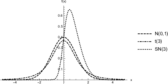
In this section, we consider three concrete forms of error distribution: a normal distribution, a t-distribution and a skew-normal distribution. A normal distribution is a theoretically basic error distribution. We are interested in how the fat tail property of a tt-distribution or the skewness of a skew-normal distribution affects the (approximated) E​D𝛼\overset{\alpha}{E\!D}. For contrasting these properties, we choose 3 for the d.f. of the tt distribution and 3 for the shape parameter of the skew-normal distribution. Figure 2 is the graph of the p.d.f.’s of the three error distributions; the standard normal distribution (N⁡(0,1)N(0,1)), the t-distribution with the d.f. of 3 (t⁡(3)t(3)), the skew-normal distribution with the shape parameter of 3 (S​N​(3)SN(3)).

Refer to caption
Figure 2: p.d.f.’s of three error distributions.

E​D𝛼\overset{\alpha}{E\!D} also depends on the moments of xx. As we can see from the definition (30)–(35), the maximum order of the joint moments of xx is four that appear in the expansion of E​D𝛼\overset{\alpha}{E\!D} up to the n−2n^{-2} order. In this section, we consider the homogeneous case where the distribution of x=(x1,…,xp)x=(x_{1},\ldots,x_{p}) is invariant w.r.t. any permutation of the elements. This is not practical but this case helps us observe the effect of the dimension pp, so called "the curse of dimension".

Here we define the notations of the homogeneous moments of xx as follows. For all distinguished i,j,k,l⁡(1≤i,j,k,l≤p)i,j,k,l\ (1\leq i,j,k,l\leq p),

m4≜E⁡[xi4],m31≜E⁡[xi3​xj],m22≜E⁡[xi2​xj2],\displaystyle m_{4}\triangleq E[x_{i}^{4}],\ m_{31}\triangleq E[x_{i}^{3}x_{j}],\ m_{22}\triangleq E[x_{i}^{2}x_{j}^{2}],
m211≜E⁡[xi2​xj​xk],m1111≜E⁡[xi​xj​xk​xl],\displaystyle m_{211}\triangleq E[x_{i}^{2}x_{j}x_{k}],\ m_{1111}\triangleq E[x_{i}x_{j}x_{k}x_{l}], (78)
m3≜E⁡[xi3],m21≜E⁡[xi2​xj],m111≜E⁡[xi​xj​xk],\displaystyle m_{3}\triangleq E[x_{i}^{3}],\ m_{21}\triangleq E[x_{i}^{2}x_{j}],\ m_{111}\triangleq E[x_{i}x_{j}x_{k}], (79)
m2≜E⁡[xi2]=1,m11≜E⁡[xi​xj]=0,\displaystyle m_{2}\triangleq E[x_{i}^{2}]=1,\ m_{11}\triangleq E[x_{i}x_{j}]=0, (80)
m1≜E⁡[xi]=0,\displaystyle m_{1}\triangleq E[x_{i}]=0, (81)
m0≜E⁡[x0]=1.\displaystyle m_{0}\triangleq E[x_{0}]=1. (82)

Under these homogeneous moments, we can state the approximated E​D𝛼\overset{\alpha}{E\!D} explicitly for each error distribution as a function of n,p,αn,p,\alpha and these moments . The result is given in the following subsections.

We used the following four distributions of xx as specific examples of the moments of xx when we want to analyze the approximated E​D𝛼\overset{\alpha}{E\!D} in a more concrete form:

  1. 1.

    The standard pp-dimensional normal distributions, Np​(0,Ip)N_{p}(0,I_{p})

    m4=3,m31=0,m22=1,m211=0,m1111=0,\displaystyle m_{4}=3,\ m_{31}=0,\ m_{22}=1,\ m_{211=0},\ m_{1111}=0,
    m3=0,m21=0,m111=0.\displaystyle m_{3}=0,\ m_{21}=0,\ m_{111}=0.
  2. 2.

    The standard pp-dimensional tt-distribution, tp​(0,Ip,ν)t_{p}(0,I_{p},\nu), that is, the pp dimensional multivariate tt-distribution with zero mean vector, the unit matrix as the scale matrix and the degree of freedom ν\nu. Its p.d.f. is given by

    h(x)∝(1+ν−1∑i=1pxi2)−(ν+p)/2h(x)\varpropto\Bigl(1+\nu^{-1}\sum_{i=1}^{p}x_{i}^{2}\Bigr)^{-(\nu+p)/2}

    Note that E[xi]=0,i=1,…,pE[x_{i}]=0,\ i=1,\ldots,p and

    C​o​v​(xi,xj)=E⁡[xi​xj]={ν/(ν−2) if i=j,0 if i≠j.Cov(x_{i},x_{j})=E[x_{i}x_{j}]=\begin{cases}\nu/(\nu-2)&\text{ if $i=j$,}\\ 0&\text{ if $i\neq j$.}\end{cases}

    for ν>2\nu>2. Therefore after the normalization (2), we have

    E⁡[xi2​xj2]={3​(ν−2)/(ν−4) if i=j,(ν−2)/(ν−4) if i≠j,E[x_{i}^{2}x_{j}^{2}]=\begin{cases}3(\nu-2)/(\nu-4)&\text{ if $i=j$,}\\ (\nu-2)/(\nu-4)&\text{ if $i\neq j$,}\end{cases}

    under the condition ν>4.\nu>4. Notice that the effect of the fourth moment is enhanced by (ν−2)/(ν−4)(\nu-2)/(\nu-4) compared to the case x∼Np​(0,Ip)x\sim N_{p}(0,I_{p}). We want to check the effect of the fat tail property of a tt-distribution. Here we put ν\nu as 4.2, then we have

    m4=33,m31=0,m22=11,m211=0,m1111=0,\displaystyle m_{4}=33,\ m_{31}=0,\ m_{22}=11,\ m_{211}=0,\ m_{1111}=0,
    m3=0,m21=0,m111=0.\displaystyle m_{3}=0,\ m_{21}=0,\ m_{111}=0.
  3. 3.

    A completely controlled distribution, where each xi,i=1,…,px_{i},i=1,\ldots,p is independently and identically distributed as P⁡(xi=1)=P⁡(xi=−1)=1/2P(x_{i}=1)=P(x_{i}=-1)=1/2.

    m4=1,m31=0,m22=1,m211=0,m1111=0,\displaystyle m_{4}=1,\ m_{31}=0,\ m_{22}=1,\ m_{211}=0,\ m_{1111}=0,
    m3=0,m21=0,m111=0.\displaystyle m_{3}=0,\ m_{21}=0,\ m_{111}=0.
  4. 4.

    Pareto distributions, where each xi,i=1,…,px_{i},i=1,\ldots,p is independently and identically distributed as P⁡(b)P(b), Pareto distributions with Pareto index bb. Its p.d.f. is given by

    h⁡(x)={∏i=1pb​xi−(b+1)if xi>1 for i=1,…,p,0otherwise.h(x)=\begin{cases}\prod_{i=1}^{p}bx_{i}^{-(b+1)}&\text{if $x_{i}>1$ for $i=1,\ldots,p,$}\\ 0&\text{otherwise.}\end{cases}

    After the normalization (2), we have

    m3\displaystyle m_{3} =Skewness of P(b)=2​(b+1)b−3​b−2b,b>3,\displaystyle=\text{Skewness of P(b)}=\frac{2(b+1)}{b-3}\sqrt{\frac{b-2}{b}},\quad b>3,
    m4\displaystyle m_{4} =Kurtosis of P(b)=6​(b3+b2−6​b−2)b​(b−3)​(b−4)+3b>4.\displaystyle=\text{Kurtosis of P(b)}=\frac{6\left(b^{3}+b^{2}-6b-2\right)}{b(b-3)(b-4)}+3\quad b>4.

    We are interested in the effect of the strong skewness and heavy tail of Pareto distribution. Here we put bb as 4.2. Consequently

    m4=812921,m31=0,m22=1,m211=0,m1111=0,\displaystyle m_{4}=\frac{8129}{21},\ m_{31}=0,\ m_{22}=1,\ m_{211}=0,\ m_{1111}=0,
    m3=2663​231,m21=0,m111=0.\displaystyle m_{3}=\frac{26}{63}\sqrt{231},\ m_{21}=0,\ m_{111}=0.

3.1 Normal Error Term Distribution

Suppose that the distribution of ϵ\epsilon is the standard normal distribution, that is,

f⁡(y)=12​π​exp⁡(−y22).f(y)=\frac{1}{\sqrt{2\pi}}\exp\Bigl(-\frac{y^{2}}{2}\Bigr).

Since

log⁡f⁡(y)=−12​log⁡(2​π)−y22,\displaystyle\log f(y)=-\frac{1}{2}\log(2\pi)-\frac{y^{2}}{2},
d​log⁡f​(y)d​y=−y,d2​log⁡f​(y)d​y2=−1,d3​log⁡f​(y)d​y3=0,\displaystyle\frac{d\log f(y)}{dy}=-y,\qquad\frac{d^{2}\log f(y)}{dy^{2}}=-1,\qquad\frac{d^{3}\log f(y)}{dy^{3}}=0,

we have for 0≤i,j,k,l≤40\leq i,j,k,l\leq 4,

η⁡[i,j,k,l]\displaystyle\eta[i,j,k,l] =12​π​∫−∞∞0i​(−1)(j+k)​yk+l​exp⁡(−y22)​𝑑y\displaystyle=\frac{1}{\sqrt{2\pi}}\int_{-\infty}^{\infty}0^{i}(-1)^{(j+k)}y^{k+l}\exp\Bigl(-\frac{y^{2}}{2}\Bigr)dy
={0 if i≥1,0 if i=0 and k+l is odd,(−1)(j+k)​(k+l−1)!! if i=0 and k+l is even,\displaystyle=\begin{cases}0&\text{ if $i\geq 1$,}\\ 0&\text{ if $i=0$ and $k+l$ is odd,}\\ (-1)^{(j+k)}(k+l-1)!!&\text{ if $i=0$ and $k+l$ is even},\end{cases} (83)

where −1!!=1, 1!!=1, 3!!=3⋅1, 5!!=5⋅3⋅1,⋯.-1!!=1,\ 1!!=1,\ 3!!=3\cdot 1,\ 5!!=5\cdot 3\cdot 1,\cdots.

Skipping long calculation (See Appendix B for the calculation procedure using Mathematica [6]. ), we give the final result in three different expressions for n−2n^{-2} order term (each expression focuses on respectively α\alpha, the moments of xx, pp).

E​D𝛼\displaystyle\overset{\alpha}{E\!D}
=p+22​n\displaystyle=\frac{p+2}{2n}
+196​n2​(α2​(84+(48−9​m22+9​m4)​p+9​m22​p2)CLOSE\displaystyle\quad+\frac{1}{96n^{2}}\Bigl(\alpha^{2}\bigl(84+(48-9m_{22}+9m_{4})p+9m_{22}p^{2}\bigr)
−8​α​(−25−3​(6+m22−m4)​p+3​(−1+m22)​p2)\displaystyle\qquad-8\alpha\bigl(-25-3(6+m_{22}-m_{4})p+3(-1+m_{22})p^{2}\bigr)
OPEN+300+240​p+81​m22​p−81​m4​p+48​p2−81​m22​p2)\displaystyle\qquad+300+240p+81m_{22}p-81m_{4}p+48p^{2}-81m_{22}p^{2}\Bigr)
+o⁡(n−2)\displaystyle\qquad+o(n^{-2}) (84)
=p+22​n\displaystyle=\frac{p+2}{2n}
+196​n2​(3​p​(−27−8​α+3​α2)​m4+3​p​(p−1)​(−27−8​α+3​α2)​m22CLOSE\displaystyle\quad+\frac{1}{96n^{2}}\Bigl(3p(-27-8\alpha+3\alpha^{2})m_{4}+3p(p-1)(-27-8\alpha+3\alpha^{2})m_{22}
4​α2​(12​p+21)+4​α​(6​p2+36​p+50)\displaystyle\hskip 85.35826pt4\alpha^{2}(12p+21)+4\alpha(6p^{2}+36p+50)
OPEN+4​(12​p2+60​p+75))\displaystyle\hskip 85.35826pt+4(12p^{2}+60p+75)\Bigr)
+o⁡(n−2)\displaystyle\qquad+o(n^{-2}) (85)
=p+22​n\displaystyle=\frac{p+2}{2n}
+196​n2​((48+24​α−81​m22−24​α​m22+9​α2​m22)​p2CLOSE\displaystyle\quad+\frac{1}{96n^{2}}\Bigl((48+24\alpha-81m_{22}-24\alpha m_{22}+9\alpha^{2}m_{22})p^{2}
+(240+144​α+48​α2+81​m22+24​α​m22−9​α2​m22CLOSE\displaystyle\hskip 85.35826pt+(240+144\alpha+48\alpha^{2}+81m_{22}+24\alpha m_{22}-9\alpha^{2}m_{22}
OPEN−81​m4−24​α​m4+9​α2​m4)​p\displaystyle\hskip 85.35826pt\quad-81m_{4}-24\alpha m_{4}+9\alpha^{2}m_{4})p
OPEN+300+200​α+84​α2)\displaystyle\hskip 85.35826pt+300+200\alpha+84\alpha^{2}\Bigr)
+o⁡(n−2)\displaystyle\qquad+o(n^{-2}) (86)

The n−2n^{-2} order term has the following properties;

  1. 1.

    The maximum dimension of pp is two, hence E​D𝛼\overset{\alpha}{E\!D} is asymptotically determined by the p−np-n ratio.

  2. 2.

    Other moments than m4m_{4} and m22m_{22} do not appear.

  3. 3.

    The coefficients of m4m_{4} and m22m_{22} are non-positive when 3​α2−8​α−27≤03\alpha^{2}-8\alpha-27\leq 0, that is,

    −1.95⋯≤α≤4.62⋯.-1.95\cdots\leq\alpha\leq 4.62\cdots. (87)

    For α\alpha within this interval, the larger m22m_{22} or m4m_{4} gets, the less E​D𝛼\overset{\alpha}{E\!D} becomes. The divergences often used in statistical literature are all included in this interval: K-L divergence (α=−1\alpha=-1), K-L dual divergence (α=1\alpha=1), Hellinger Divergence (α=0\alpha=0), χ2\chi^{2} divergence (α=3\alpha=3).

Most commonly used α\alpha-divergence is Kullback-Leibler divergence given by α=−1\alpha=-1;

E​D​​−1\displaystyle\overset{\scalebox{0.6}{\!\!$-1$}}{E\!D}
=p+22​n+112​n2​(23+6​(3+m22−m4)​p+(3−6​m22)​p2)\displaystyle=\frac{p+2}{2n}+\frac{1}{12n^{2}}\Bigl(23+6(3+m_{22}-m_{4})p+(3-6m_{22})p^{2}\Bigr)
+o⁡(n−2)\displaystyle\quad+o(n^{-2}) (88)

Its "dual" divergence given by α=1\alpha=1 satisfies the relationship

D​​1[θ1:θ2]=D​​−1[θ2:θ1].\overset{\scalebox{0.6}{\!\!$1$}}{D}[\theta_{1}:\theta_{2}]=\overset{\scalebox{0.6}{\!\!$-1$}}{D}[\theta_{2}:\theta_{1}].

The risk of m.l.e. with respect to this divergence is given by;

E​D​​1\displaystyle\overset{\scalebox{0.6}{\!\!$1$}}{E\!D}
=p+22​n+112​n2​(73+6​(9+2​m22−2​m4)​p+(9−12​m22)​p2)\displaystyle=\frac{p+2}{2n}+\frac{1}{12n^{2}}\Bigl(73+6(9+2m_{22}-2m_{4})p+(9-12m_{22})p^{2}\Bigr)
+o⁡(n−2)\displaystyle\quad+o(n^{-2}) (89)

When α=0\alpha=0, the α\alpha-divergence becomes a distance, which is called Hellinger distance;

E​D​​0\displaystyle\overset{\scalebox{0.6}{\!\!$0$}}{E\!D}
=p+22​n+132​n2​(100+(80+27​m22−27​m4)​p+(16−27​m22)​p2)\displaystyle=\frac{p+2}{2n}+\frac{1}{32n^{2}}\Bigl(100+(80+27m_{22}-27m_{4})p+(16-27m_{22})p^{2}\Bigr)
+o⁡(n−2)\displaystyle\quad+o(n^{-2}) (90)

When α=3\alpha=3, it becomes χ2\chi^{2} divergence;

E​D​​3\displaystyle\overset{\scalebox{0.6}{\!\!$3$}}{E\!D}
=p+22​n+14​n2​(69+(46+3​m22−3​m4)​p+(5−3​m22)​p2)\displaystyle=\frac{p+2}{2n}+\frac{1}{4n^{2}}\Bigl(69+(46+3m_{22}-3m_{4})p+(5-3m_{22})p^{2}\Bigr)
+o⁡(n−2)\displaystyle\quad+o(n^{-2}) (91)

For each distribution of xx introduced in the beginning of Section 3, we have the following results.

  1. 1.

    x∼Np​(0,Ip)x\sim N_{p}(0,I_{p})

    E​D𝛼\displaystyle\overset{\alpha}{E\!D}
    =p+22​n\displaystyle=\frac{p+2}{2n}
    +196​n2​(α2​(84+66​p+9​p2)+8​α​(25+12​p)+300+78​p−33​p2)\displaystyle\quad+\frac{1}{96n^{2}}\Bigl(\alpha^{2}(84+66p+9p^{2})+8\alpha(25+12p)+300+78p-33p^{2}\Bigr)
    +o⁡(n−2)\displaystyle\quad+o(n^{-2}) (92)
  2. 2.

    x∼tp​(0,Ip,4.2)x\sim t_{p}(0,I_{p},4.2)

    E​D𝛼\displaystyle\overset{\alpha}{E\!D}
    =p+22​n\displaystyle=\frac{p+2}{2n}
    +196​n2​(3​α2​(28+82​p+33​p2)+8​α​(−25+48​p+30​p2)+300−1542​p−843​p2)\displaystyle\quad+\frac{1}{96n^{2}}\Bigl(3\alpha^{2}(28+82p+33p^{2})+8\alpha(-25+48p+30p^{2})+300-1542p-843p^{2}\Bigr)
    +o⁡(n−2)\displaystyle\quad+o(n^{-2}) (93)
  3. 3.

    xx is controlled.

    E​D𝛼\displaystyle\overset{\alpha}{E\!D}
    =p+22​n\displaystyle=\frac{p+2}{2n}
    +196​n2​(α2​(84+48​p+9​p2)+8​α​(25+18​p)+300+240​p−33​p2)\displaystyle\quad+\frac{1}{96n^{2}}\Bigl(\alpha^{2}(84+48p+9p^{2})+8\alpha(25+18p)+300+240p-33p^{2}\Bigr)
    +o⁡(n−2)\displaystyle\quad+o(n^{-2}) (94)
  4. 4.

    xix_{i} is i.i.d. as P⁡(4.2)P(4.2) (i=1,…,p)(i=1,\ldots,p)

    E​D𝛼\displaystyle\overset{\alpha}{E\!D}
    =p+22​n\displaystyle=\frac{p+2}{2n}
    +1672​n2​(3​α2​(196+8220​p+21​p2)−8​α​(−175+7982​p)CLOSE\displaystyle\quad+\frac{1}{672n^{2}}\Bigl(3\alpha^{2}(196+8220p+21p^{2})-8\alpha(-175+7982p)
    OPEN+3​(700−72412​p−77​p2))\displaystyle\qquad\qquad\qquad+3(700-72412p-77p^{2})\Bigr)
    +o⁡(n−2)\displaystyle\quad+o(n^{-2}) (95)

We made a numerical comparison to see the effect of the joint moments of xx. We set p=10p=10 and n=12​kn=12k, which means p−np-n ratio equals 1/k1/k since the number of the parameters of the regression model (1) equals 12 when p=10p=10. Figure 3 is the graph of the approximated E​D​​−1\overset{\scalebox{0.6}{\!\!$-1$}}{E\!D}’s corresponding to each distribution of xx above-mentioned as kk varies from 5 to 100. (The graph for the controlled distribution is always quite similar to that for the normal distribution, hence for the clarity of the figures we will omit it in every figure hereafter.) Figure 4 magnifies the part k=50,…,100.k=50,\ldots,100. We put as the benchmark the approximated E​D​​−1\overset{\scalebox{0.6}{\!\!$-1$}}{E\!D} of the binomial model B⁡(k,0.5)B(k,0.5), that is, the kk-times normal coin toss model.

Refer to caption
Figure 3: E​D−1\overset{-1}{E\!D} when ϵ∼N⁡(0,1)\epsilon\sim N(0,1)
Refer to caption
Figure 4: E​D−1\overset{-1}{E\!D} when ϵ∼N⁡(0,1)\epsilon\sim N(0,1)
Refer to caption
Figure 5: E​D−6\overset{-6}{E\!D} when ϵ∼N⁡(0,1)\epsilon\sim N(0,1)
Table 1: I.D.E. & R.S.S. for N⁡(0,1)N(0,1) error distribution
I.D.E. R.S.S.
x∼N10​(0,I10)x\sim N_{10}(0,I_{10}) * 111(10)
x∼t10​(0,I10,4.2)x\sim t_{10}(0,I_{10},4.2) * 322(40)
xx is controlled * 112(10)
xx is i.i.d.P⁡(4.2)i.i.d.P(4.2) * 741(110)

We notice that heavy tail property of Pareto distribution P⁡(4.2)P(4.2) or tt-distribution t⁡(4.2)t(4.2) decreases difficulty in estimating the parameter, especially the large m4m_{4} value 8129/21 of P⁡(4.2)P(4.2) makes the estimation easier. On the contrary, if m4m_{4} and m22m_{22} are as small as those of N10​(0,I10)N_{10}(0,I_{10}) (or the controlled distribution), then the difficulty of estimation is close to the normal coin toss.

Here we refer to the question how large sample size is required for the good approximation of E​D𝛼\overset{\alpha}{E\!D} by the expansion up to the n−2n^{-2} order term. It is very difficult to give a general answer to this question, but at least for a specific model, obviously we should not use the approximation unless it is positive or decreasing with respect to nn. For example, in Figure 3, we see that the approximation for t10t_{10} should be used for k>10k>10, namely n>120n>120.

We observed that the effects of m4m_{4} and m22m_{22} depends on α\alpha. If α\alpha is outside the interval (87), the large value of m44m_{44} or m22m_{22} enhances the difficulty of the estimation. For example, if α=−6\alpha=-6, the order of various distributions of xx is completely reversed to that for the case α=−1\alpha=-1 as we can see from Figure 5.

Now we consider I.D.E. and R.S.S. introduced in Section 2. We take Kullback-Leibler divergence (α=−1\alpha=-1) as an example. Let pp be 10. When xx is distributed as Np​(0,Ip)N_{p}(0,I_{p}), we have

E​D​​−1​(n)=6n−21712​n2.\overset{\scalebox{0.6}{\!\!$-1$}}{E\!D}(n)=\frac{6}{n}-\frac{217}{12n^{2}}.

“Indicator of the difficulty of estimation” is given as the solution of mm for the equation

12​k+112​k2​(M−1)=12​k−21712×(12​k)2\frac{1}{2k}+\frac{1}{12k^{2}}(M-1)=\frac{1}{2k}-\frac{217}{12\times(12k)^{2}}

(See (75) for the left-hand side.) Actually this quadratic equation of mm does not have the real roots. The left-hand side is always larger than the right-hand side. This means the estimation of the regression model is easier than the coin toss problem under the same p−np-n ratio.

Sample size determination is solving the next equation;

120+1400=6n−21712​n2.\frac{1}{20}+\frac{1}{400}=\frac{6}{n}-\frac{217}{12n^{2}}.

where n=111n=111 is the rounded solution. For the other distributions (joint moments) of xx, we can similarly calculate I.D.E. and R.S.S..The result is given in Table 1. "*" indicates that the equation has no solutions. The number in the parenthesis in R.S.S. shows the sample size of the binomial model in the left-hand side of (77) (see the last paragraph of Section 2.) With the sample size given by R.S.S., the p−np-n ratio of the regression model equals 12/R.S.S., while that of the coin toss model is equal to the reciprocal of the number in the parenthesis. Hence R.S.S divided by the number in the parenthesis could be another indicator. It is smaller for t10​(0,I10,4.2)t_{10}(0,I_{10},4.2) or P⁡(4.2)P(4.2) than that for N10​(0,I10)N_{10}(0,I_{10}) or the controlled distribution. The large joint moments m4m_{4}, m22m_{22} for t10​(0,I10,4.2)t_{10}(0,I_{10},4.2) or P⁡(4.2)P(4.2) make estimation easier. We can guess that the large oscillation of xx is helpful to estimate the values of β\beta. Nevertheless of these differences, in general, the estimation for the regression model under the normal error distribution is not so troublesome, since 10 times as large sample size as the dimension of the parameter guarantees relatively easy estimation.

3.2 tt Error Term Distribution

In this subsection we investigate the case where ϵ\epsilon has a tt-distribution. Since

f(y)=c(ν)(1+y2/ν)−(ν+1)/2,c(ν)=Γ((ν+1)/2)/(π​νΓ(ν/2)),f(y)=c(\nu)(1+y^{2}/\nu)^{-(\nu+1)/2},\quad c(\nu)=\Gamma((\nu+1)/2)/(\sqrt{\pi\nu}\Gamma(\nu/2)),

we have

log⁡f⁡(y)\displaystyle\log f(y) =log⁡c⁡(ν)−ν+12​log⁡(1+y2ν),\displaystyle=\log c(\nu)-\frac{\nu+1}{2}\log(1+\frac{y^{2}}{\nu}),
dd​y​log⁡f​(y)\displaystyle\frac{d}{dy}\log f(y) =−(ν+1)​yν+y2,\displaystyle=-(\nu+1)\frac{y}{\nu+y^{2}},
d2d​y2​log⁡f​(y)\displaystyle\frac{d^{2}}{dy^{2}}\log f(y) =(ν+1)​y2−ν(ν+y2)2,\displaystyle=(\nu+1)\frac{y^{2}-\nu}{(\nu+y^{2})^{2}},
d3d​y3​log⁡f​(y)\displaystyle\frac{d^{3}}{dy^{3}}\log f(y) =2​(ν+1)​y​3​ν−y2(ν+y2)3.\displaystyle=2(\nu+1)y\frac{3\nu-y^{2}}{(\nu+y^{2})^{3}}.

If we put y~\tilde{y} as ν+y2\nu+y^{2}, then

(d3d​y3​log⁡f⁡(y))i​(d2d​y2​log⁡f⁡(y))j​(dd​y​log⁡f⁡(y))k​yl\displaystyle\Bigl(\frac{d^{3}}{dy^{3}}\log f(y)\Bigr)^{i}\Bigl(\frac{d^{2}}{dy^{2}}\log f(y)\Bigr)^{j}\Bigl(\frac{d}{dy}\log f(y)\Bigr)^{k}y^{l}
=((−1)i​2i​(ν+1)i​yi​(y2−3​ν)i​y~−3​i)​((ν+1)j​(y2−ν)j​y~−2​j)​((−1)k​(ν+1)k​yk​y~−k)​yl\displaystyle=\Bigl((-1)^{i}2^{i}(\nu+1)^{i}y^{i}(y^{2}-3\nu)^{i}\tilde{y}^{-3i}\Bigr)\Bigl((\nu+1)^{j}(y^{2}-\nu)^{j}\tilde{y}^{-2j}\Bigr)\Bigl((-1)^{k}(\nu+1)^{k}y^{k}\tilde{y}^{-k}\Bigr)y^{l}
=2i​(−1)i+k​(ν+1)i+j+k​yi+k+l​(y2−3​ν)i​(y2−ν)j​y~−(3​i+2​j+k)\displaystyle=2^{i}(-1)^{i+k}(\nu+1)^{i+j+k}y^{i+k+l}(y^{2}-3\nu)^{i}(y^{2}-\nu)^{j}\tilde{y}^{-(3i+2j+k)}
=2i​(−1)i+k​(ν+1)i+j+k​yi+k+l\displaystyle=2^{i}(-1)^{i+k}(\nu+1)^{i+j+k}y^{i+k+l}
×(∑s=0iy2​s​(−3​ν)i−s​Csi)​(∑t=0jy2​t​(−ν)j−t​Ctj)​y~−(3​i+2​j+k)\displaystyle\quad\times\Bigl(\sum_{s=0}^{i}y^{2s}(-3\nu)^{i-s}{}_{i}C_{s}\Bigr)\Bigl(\sum_{t=0}^{j}y^{2t}(-\nu)^{j-t}{}_{j}C_{t}\Bigr)\tilde{y}^{-(3i+2j+k)}
=∑s=0i∑t=0j2i​(−1)2​i+j+k−s−t​(ν+1)i+j+k​νi+j−s−t​yi+k+l+2​s+2​t​Csi​Ctj​y~−(3​i+2​j+k).\displaystyle=\sum_{s=0}^{i}\sum_{t=0}^{j}2^{i}(-1)^{2i+j+k-s-t}(\nu+1)^{i+j+k}\nu^{i+j-s-t}y^{i+k+l+2s+2t}\,{}_{i}C_{s}\,{}_{j}C_{t}\,\tilde{y}^{-(3i+2j+k)}.

Consequently

η[i,j,k,,l]\displaystyle\eta[i,j,k,,l]
=∑s=0i∑t=0j2i​(−1)2​i+j+k−s−t​(ν+1)i+j+k​ν−s−t−2​i−j−k​Csi​Ctj\displaystyle=\sum_{s=0}^{i}\sum_{t=0}^{j}2^{i}(-1)^{2i+j+k-s-t}(\nu+1)^{i+j+k}\nu^{-s-t-2i-j-k}\,{}_{i}C_{s}\,{}_{j}C_{t}
×c⁡(ν)​H​(i+k+l+2​s+2​t,ν+6​i+4​j+2​k),\displaystyle\quad\times c(\nu)H(i+k+l+2s+2t,\nu+6i+4j+2k), (96)

where

H⁡(a,b)\displaystyle H(a,b) ≜∫−∞∞ya(1+y2/ν)−(b+1)/2dy\displaystyle\triangleq\int_{-\infty}^{\infty}y^{a}(1+y^{2}/\nu)^{-(b+1)/2}dy
=∫−∞∞ya(1+y2​(b/v)b)−(b+1)/2dy\displaystyle=\int_{-\infty}^{\infty}y^{a}\biggl(1+\frac{y^{2}(b/v)}{b}\biggr)^{-(b+1)/2}dy
=∫−∞∞y~a(νb)a/2(1+y~2b)−(b+1)/2(νb)1/2dy~,y~≜ybv\displaystyle=\int_{-\infty}^{\infty}\tilde{y}^{a}\biggl(\frac{\nu}{b}\biggr)^{a/2}\biggl(1+\frac{\tilde{y}^{2}}{b}\biggr)^{-(b+1)/2}\biggl(\frac{\nu}{b}\biggr)^{1/2}d\tilde{y},\qquad\tilde{y}\triangleq y\sqrt{\frac{b}{v}}
=(νb)(a+1)/2∫−∞∞y~a(1+y~2b)−(b+1)/2dy~\displaystyle=\biggl(\frac{\nu}{b}\biggr)^{(a+1)/2}\int_{-\infty}^{\infty}{\tilde{y}}^{a}\biggl(1+\frac{\tilde{y}^{2}}{b}\biggr)^{-(b+1)/2}d\tilde{y}
=(νb)(a+1)/2​1c⁡(b)​E​[ta],t∼t⁡(b)\displaystyle=\biggl(\frac{\nu}{b}\biggr)^{(a+1)/2}\frac{1}{c(b)}E[t^{a}],\quad t\sim t(b)
={0, if 0<a<b, and a is an odd number,ν(a+1)/2​Γ⁡((a+1)/2)​Γ​((b−a)/2)Γ⁡((b+1)/2), if 0<a<b, and a is a even number.\displaystyle=\begin{cases}0,&\text{ if $0<a<b$, and $a$ is an odd number,}\\ \nu^{(a+1)/2}\>\frac{\Gamma((a+1)/2)\Gamma((b-a)/2)}{\Gamma((b+1)/2)},&\text{ if $0<a<b$, and $a$ is a even number.}\end{cases}

If we insert these results, we get E​D𝛼\overset{\alpha}{E\!D} as a function of p,n,α,νp,n,\alpha,\nu and the joint moments of xx. We are interested in how E​D𝛼\overset{\alpha}{E\!D} is effected by a long tail error distribution compared to the standard normal distribution, hence we set ν\nu as 3. (Mathematica program for a general ν\nu is available in Appendix B) We have the following result;

E​D𝛼\displaystyle\overset{\alpha}{E\!D}
=p+22​n\displaystyle=\frac{p+2}{2n}
+1384​n2​(6​α2​(13+(10−3​m22+3​m4)​p+3​m22​p2)CLOSE\displaystyle\qquad+\frac{1}{384n^{2}}\Bigl(6\alpha^{2}\left(13+(10-3m_{22}+3m_{4})p+3m_{22}p^{2}\right)
−2​α​(−77+(−72−51​m22+51​m4)​p+3​(−5+17​m22)​p2)\displaystyle\hskip 85.35826pt-2\alpha\left(-77+(-72-51m_{22}+51m_{4})p+3(-5+17m_{22})p^{2}\right)
OPEN+3​(287+(296+90​m22−90​m4)​p+(65−90​m22)​p2))\displaystyle\hskip 85.35826pt+3\left(287+(296+90m_{22}-90m_{4})p+(65-90m_{22})p^{2}\right)\Bigr)
+o⁡(n−2)\displaystyle\qquad+o(n^{-2}) (97)
=p+22​n\displaystyle=\frac{p+2}{2n}
+1384​n2​(6​p​(−45−17​α+3​α2)​m4+6​p​(p−1)​(−45−17​α+3​α2)​m22CLOSE\displaystyle\quad+\frac{1}{384n^{2}}\Bigl(6p(-45-17\alpha+3\alpha^{2})m_{4}+6p(p-1)(-45-17\alpha+3\alpha^{2})m_{22}
+α2​(78+60​p)+α⁡(154+144​p+30​p2)\displaystyle\hskip 71.13188pt+\alpha^{2}(78+60p)+\alpha(154+144p+30p^{2})
OPEN+861+888​p+195​p2)\displaystyle\hskip 71.13188pt+861+888p+195p^{2}\Bigr)
+o⁡(n−2)\displaystyle\qquad+o(n^{-2}) (98)
=p+22​n\displaystyle=\frac{p+2}{2n}
+1384​n2​((195+30​α−270​m22−102​α​m22+18​α2​m22)​p2CLOSE\displaystyle\quad+\frac{1}{384n^{2}}\Bigl((195+30\alpha-270m_{22}-102\alpha m_{22}+18\alpha^{2}m_{22})p^{2}
+(888+144​α+60​α2+270​m22+102​α​m22−18​α2​m22CLOSE\displaystyle\hskip 71.13188pt+(888+144\alpha+60\alpha^{2}+270m_{22}+102\alpha m_{22}-18\alpha^{2}m_{22}
OPEN−270​m4−102​α​m4+18​α2​m4)​p\displaystyle\hskip 71.13188pt\qquad-270m_{4}-102\alpha m_{4}+18\alpha^{2}m_{4})p
OPEN+861+154​α+78​α2)\displaystyle\hskip 71.13188pt+861+154\alpha+78\alpha^{2}\Bigr)
+o⁡(n−2)\displaystyle\qquad+o(n^{-2}) (99)

The n−2n^{-2} order term has similar properties as in the case of N⁡(0,1)N(0,1).

  1. 1.

    The dimension of pp is two, hence E​D𝛼\overset{\alpha}{E\!D} is asymptotically determined by the p−np-n ratio.

  2. 2.

    Other moments than m4m_{4} and m22m_{22} do not appear.

  3. 3.

    The coefficients of m4m_{4} and m22m_{22} are non-positive when 3​α2−17​α−45≤03\alpha^{2}-17\alpha-45\leq 0, that is,

    −1.97⋯≤α≤7.63⋯.-1.97\cdots\leq\alpha\leq 7.63\cdots. (100)

    For α\alpha within this interval, the larger m22m_{22} or m4m_{4} gets, the less E​D𝛼\overset{\alpha}{E\!D} becomes. The divergences often used in statistical literature are all included in this interval.

We noticed that if the error term distribution is the standard normal distribution (see (85)) or t⁡(3)t(3) distribution (see (98)), only m4m_{4} and m22m_{22} among the moments (78) and (79) appear in the asymptotic expansion of E​D𝛼\overset{\alpha}{E\!D} up to the n−2n^{-2} order. On this phenomena, we have the following general result.

Proposition 1.

If the error term distribution is quadratic, namely f⁡(ϵ)=g⁡(ϵ2)f(\epsilon)=g(\epsilon^{2}) for some function g⁡(⋅)g(\cdot), then the asymptotic expansion of E​D𝛼\overset{\alpha}{E\!D} up to the order n−2n^{-2} includes only m4m_{4} and m22m_{22} among the third and forth order joint moments of xx.

<Proof> From (11), we notice that the third or forth order moments of xx in the expansion of E​D𝛼\overset{\alpha}{E\!D} up to the order n−2n^{-2} are generated from the terms m⁡[i,j,k,l]m[i,j,k,l] and m⁡[i,j,k]​m​[s,t,u]m[i,j,k]m[s,t,u].

The forth order moments arise from m⁡[i,j,k,l]​(1≤i,j,k,l≤p)m[i,j,k,l](1\leq i,j,k,l\leq p) in L​11L11 to L​15L15. Since m⁡[i,j,k,l]m[i,j,k,l] is multiplied with gi​j​gk​lg^{ij}g^{kl} as in (11), and gi​jg^{ij} vanishes unless i=ji=j, the possible moments coming from E⁡[xi​xj​xk​xl]E[x_{i}x_{j}x_{k}x_{l}] are only m4m_{4} and m22m_{22}.

On the other hand, m⁡[i,j,k]​m​[s,t,u]m[i,j,k]m[s,t,u] come from either term of L​21,…,L​26L21,\ldots,L26. We notice that if the third moments are generated from these terms, they are always multiplied with η⁡[0,1,1,0]\eta[0,1,1,0] or η⁡[0,0,3,0]\eta[0,0,3,0]. (See (30), (31).) If f⁡(ϵ)=g⁡(ϵ2)f(\epsilon)=g(\epsilon^{2}), then we have

dd​y​log⁡f​(y)=2​y​g′​(y2)g⁡(y2),\displaystyle\frac{d}{dy}\log f(y)=2y\frac{g^{\prime}(y^{2})}{g(y^{2})},
d2d​y2​log⁡f⁡(y)=2g2​(y2)​(g′​(y2)+2​y2​g′′​(y2)​g​(y2)+2​y2​(g′​(y2))2).\displaystyle\frac{d^{2}}{dy^{2}}\log f(y)=\frac{2}{g^{2}(y^{2})}\Bigl(g^{\prime}(y^{2})+2y^{2}g^{\prime\prime}(y^{2})g(y^{2})+2y^{2}(g^{\prime}(y^{2}))^{2}\Bigr).

Therefore η⁡[0,1,1,0]\eta[0,1,1,0] and η⁡[0,0,3,0]\eta[0,0,3,0] vanishes. Q.E.D.
Typical four cases α=−1,1,0,3\alpha=-1,1,0,3 are given as follows;

E​D​​−1=p+22​n\displaystyle\overset{\scalebox{0.6}{\!\!$-1$}}{E\!D}=\frac{p+2}{2n}
+1384​n2​(785+6​(134+25​m22−25​m4)​p+(165−150​m22)​p2)+o⁡(n−2),\displaystyle\qquad\quad+\frac{1}{384n^{2}}\Bigl(785+6(134+25m_{22}-25m_{4})p+(165-150m_{22})p^{2}\Bigr)+o(n^{-2}), (101)
E​D​​1=p+22​n\displaystyle\overset{\scalebox{0.6}{\!\!$1$}}{E\!D}=\frac{p+2}{2n}
+1384​n2​(1093+6​(182+59​m22−59​m4)​p+(225−354​m22)​p2)+o⁡(n−2),\displaystyle\qquad\quad+\frac{1}{384n^{2}}\Bigl(1093+6(182+59m_{22}-59m_{4})p+(225-354m_{22})p^{2}\Bigr)+o(n^{-2}), (102)
E​D​​0=p+22​n\displaystyle\overset{\scalebox{0.6}{\!\!$0$}}{E\!D}=\frac{p+2}{2n}
+1384​n2​(287+(296+90​m22−90​m4)​p+(65−90​m22)​p2)+o⁡(n−2),\displaystyle\qquad\quad+\frac{1}{384n^{2}}\Bigl(287+(296+90m_{22}-90m_{4})p+(65-90m_{22})p^{2}\Bigr)+o(n^{-2}), (103)
E​D​​3=p+22​n\displaystyle\overset{\scalebox{0.6}{\!\!$3$}}{E\!D}=\frac{p+2}{2n}
+1128​n2​(675+2​(310+69​m22−69​m4)​p+(95−138​m22)​p2)+o⁡(n−2).\displaystyle\qquad\quad+\frac{1}{128n^{2}}\Bigl(675+2(310+69m_{22}-69m_{4})p+(95-138m_{22})p^{2}\Bigr)+o(n^{-2}). (104)

For each distribution (moments) of xx introduced in Section 2, we have the following results.

  1. 1.

    x∼Np​(0,Ip)x\sim N_{p}(0,I_{p})

    E​D𝛼\displaystyle\overset{\alpha}{E\!D}
    =p+22​n\displaystyle=\frac{p+2}{2n}
    +1384​n2​(6​α2​(13+16​p+3​p2)−2​α​(−77+30​p+36​p2)CLOSE\displaystyle\quad+\frac{1}{384n^{2}}\Bigl(6\alpha^{2}(13+16p+3p^{2})-2\alpha(-77+30p+36p^{2})
    OPEN861+348​p−75​p2)+o⁡(n−2)\displaystyle\qquad\qquad\qquad 861+348p-75p^{2}\Bigr)+o(n^{-2}) (105)
  2. 2.

    x∼tp​(0,Ip,4.2)x\sim t_{p}(0,I_{p},4.2)

    E​D𝛼\displaystyle\overset{\alpha}{E\!D}
    =p+22​n\displaystyle=\frac{p+2}{2n}
    +1384​n2​(6​α2​(13+76​p+33​p2)−14​α​(−11+150​p+78​p2)CLOSE\displaystyle\quad+\frac{1}{384n^{2}}\Bigl(6\alpha^{2}(13+76p+33p^{2})-14\alpha(-11+150p+78p^{2})
    OPEN3​(287−1684​p−925​p2))+o⁡(n−2)\displaystyle\qquad\qquad\qquad 3(287-1684p-925p^{2})\Bigr)+o(n^{-2}) (106)
  3. 3.

    xx is controlled.

    E​D𝛼\displaystyle\overset{\alpha}{E\!D}
    =p+22​n\displaystyle=\frac{p+2}{2n}
    +1384​n2​(6​α2​(13+10​p+3​p2)+α⁡(154+144​p−72​p2)CLOSE\displaystyle\quad+\frac{1}{384n^{2}}\Bigl(6\alpha^{2}(13+10p+3p^{2})+\alpha(154+144p-72p^{2})
    OPEN861+888​p−75​p2)+o⁡(n−2)\displaystyle\qquad\qquad\qquad 861+888p-75p^{2}\Bigr)+o(n^{-2}) (107)
  4. 4.

    xix_{i} is i.i.d. as P⁡(4.2)P(4.2) (i=1,…,p)(i=1,\ldots,p)

    E​D𝛼\displaystyle\overset{\alpha}{E\!D}
    =p+22​n\displaystyle=\frac{p+2}{2n}
    +12688​n2​(6​α2​(91+8178​p+21​p2)−2​α​(−539+137332​p+252​p2)CLOSE\displaystyle\quad+\frac{1}{2688n^{2}}\Bigl(6\alpha^{2}(91+8178p+21p^{2})-2\alpha(-539+137332p+252p^{2})
    OPEN3​(2009−241168​p−175​p2))+o⁡(n−2)\displaystyle\qquad\qquad\qquad 3(2009-241168p-175p^{2})\Bigr)+o(n^{-2}) (108)

We made a numerical comparison under the condition p=10p=10 and n=12​kn=12k, which means p−np-n ratio equals 1/k1/k. Figure 6 is the graph of the approximated E​D​​−1\overset{\scalebox{0.6}{\!\!$-1$}}{E\!D}’s corresponding to each distribution above-mentioned except for the controlled distribution as kk varies from 5 to 100. Figure 7 magnifies the part of kk from 40 to 50. We put as the benchmark the approximated E​D​​−1\overset{\scalebox{0.6}{\!\!$-1$}}{E\!D} of the binomial model B⁡(k,0.5)B(k,0.5).

Just like the case of N⁡(0,1)N(0,1), heavy tail property of Pareto distribution P⁡(4.2)P(4.2) or tt-distribution t⁡(4.2)t(4.2) eases difficulty in estimating the parameter. On the contrary, if m4m_{4} and m22m_{22} are as small as those of N⁡(0,1)N(0,1) (or the controlled distribution), then the difficulty of estimation is close to the normal coin toss.

It was also observed that the effects of m4m_{4} and m22m_{22} depends on α\alpha. If α\alpha is outside the interval (100), the large value of m44m_{44} or m22m_{22} enhances the difficulty of the estimation. For example, see Figure 8 for α=−6\alpha=-6, where the E​D−6\overset{-6}{E\!D} for the tt or Pareto distribution is larger than that of the normal distribution.

We considered I.D.E. and R.S.S. w.r.t. Kullback-Leibler divergence under the condition p=10p=10 for each distribution of xx. Table 2 shows the result.The same comments hold as in the case of N⁡(0,1)N(0,1). The large value of m4m_{4} or m22m_{22} of the tt-distribution or Pareto distribution makes the estimation easier compared to the normal distribution or the controlled distribution. Generally speaking, irrespective of the above difference, the estimation of the regression model under tt-distribution error is not so hard. With 10 times as large sample size as the parameter dimension, we can estimate the parameter without much trouble.

Refer to caption
Figure 6: E​D−1\overset{-1}{E\!D} when ϵ∼t⁡(3)\epsilon\sim t(3)
Refer to caption
Figure 7: E​D−1\overset{-1}{E\!D} when ϵ∼t⁡(3)\epsilon\sim t(3)
Refer to caption
Figure 8: E​D−6\overset{-6}{E\!D} when ϵ∼t⁡(3)\epsilon\sim t(3)
Table 2: I.D.E. & R.S.S. for t⁡(3)t(3) error distribution
I.D.E. R.S.S.
x∼N10​(0,I10)x\sim N_{10}(0,I_{10}) * 117(10)
x∼t10​(0,I10,4.2)x\sim t_{10}(0,I_{10},4.2) * 246(30)
xx is controlled * 118(10)
xx is i.i.d.P⁡(4.2)i.i.d.P(4.2) * 689(90)

3.3 Skew-Normal Error Term Distribution

In this subsection, we take a skew-normal distribution as an error term distribution so that we investigate how the skewness of error effects E​D𝛼.\overset{\alpha}{E\!D}. Suppose that f⁡(y)f(y) is given by

f⁡(y)=2​ϕ​(y)​Φ​(b​y),f(y)=2\phi(y)\Phi(by),

where ϕ⁡(y)\phi(y) is the p.d.f. of the standard normal distribution, and Φ⁡(y)\Phi(y) is its cumulative distribution function. This is the p.d.f. of the (standard) skew-normal distribution with the shape parameter bb. If bb is positive (negative), the distribution is right (left) skewed. When b=0b=0, it is the standard normal distribution.

For this distribution, we have

log⁡f⁡(y)\displaystyle\log f(y) =log⁡2+log⁡ϕ⁡(y)+log⁡Φ⁡(b​y),\displaystyle=\log 2+\log\phi(y)+\log\Phi(by),
dd​y​log⁡f​(y)\displaystyle\frac{d}{dy}\log f(y) =−y+b​ϕ​(b​y)Φ⁡(b​y),\displaystyle=-y+\frac{b\phi(by)}{\Phi(by)},
d2d​y2​log⁡f​(y)\displaystyle\frac{d^{2}}{dy^{2}}\log f(y) =−1−b2​ϕ2​(b​y)Φ2​(b​y)+b2​ϕ′​(b​y)Φ⁡(b​y)=−1−b2​ϕ2​(b​y)Φ2​(b​y)−b3​y​ϕ⁡(b​y)Φ⁡(b​y),\displaystyle=-1-b^{2}\frac{\phi^{2}(by)}{\Phi^{2}(by)}+\frac{b^{2}\phi^{\prime}(by)}{\Phi(by)}=-1-b^{2}\frac{\phi^{2}(by)}{\Phi^{2}(by)}-b^{3}y\frac{\phi(by)}{\Phi(by)},
d3d​y3​log⁡f​(y)\displaystyle\frac{d^{3}}{dy^{3}}\log f(y) =2​b3​ϕ3​(b​y)Φ3​(b​y)−2​b3​ϕ⁡(b​y)​ϕ′​(b​y)Φ2​(b​y)−b3​ϕ⁡(b​y)​ϕ′​(b​y)Φ2​(b​y)+b3​ϕ′′​(b​y)Φ⁡(b​y)\displaystyle=2b^{3}\frac{\phi^{3}(by)}{\Phi^{3}(by)}-2b^{3}\frac{\phi(by)\phi^{\prime}(by)}{\Phi^{2}(by)}-b^{3}\frac{\phi(by)\phi^{\prime}(by)}{\Phi^{2}(by)}+b^{3}\frac{\phi^{\prime\prime}(by)}{\Phi(by)}
=2​b3​ϕ3​(b​y)Φ3​(b​y)−3​b3​ϕ⁡(b​y)​ϕ′​(b​y)Φ2​(b​y)+b3​ϕ′′​(b​y)Φ⁡(b​y)\displaystyle=2b^{3}\frac{\phi^{3}(by)}{\Phi^{3}(by)}-3b^{3}\frac{\phi(by)\phi^{\prime}(by)}{\Phi^{2}(by)}+b^{3}\frac{\phi^{\prime\prime}(by)}{\Phi(by)}
=b3​(2​ϕ3​(b​y)Φ3​(b​y)+3​b​y​ϕ2​(b​y)Φ2​(b​y)+(b2​y2−1)​ϕ⁡(b​y)Φ⁡(b​y))\displaystyle=b^{3}\biggl(2\frac{\phi^{3}(by)}{\Phi^{3}(by)}+3by\frac{\phi^{2}(by)}{\Phi^{2}(by)}+(b^{2}y^{2}-1)\frac{\phi(by)}{\Phi(by)}\biggr)

If we insert these results into the definition (20), we get the formal form of η⁡[i,j,k,l]\eta[i,j,k,l]. However, since the value of η⁡[i,j,k,l]\eta[i,j,k,l] can not be gained theoretically, we have to calculate it numerically after a specific value of bb is chosen. Here we put b=3b=3 for a relatively strong right skewness. The asymptotic expansion of E​D𝛼\overset{\alpha}{E\!D} is given as follows (the numbers are rounded off to three decimal place).

E​D𝛼\displaystyle\overset{\alpha}{E\!D}
=p+22​n\displaystyle=\frac{p+2}{2n}
+1n2​(α2​(0.175​m22​p2+(0.175​m4−0.175​m22+0.689)​p+0.988)CLOSE\displaystyle\quad+\frac{1}{n^{2}}\Bigl(\alpha^{2}\bigl(0.175m_{22}p^{2}+(0.175m_{4}-0.175m_{22}+0.689)p+0.988\bigr)
+α⁡((0.087​m1112+0.130​m212)​p3CLOSE\displaystyle\qquad\qquad+\alpha\bigl((0.087m_{111}^{2}+0.130m_{21}^{2})p^{3}
+(0.385−0.260​m1112−0.430​m22+0.260​m21​m3)​p2\displaystyle\qquad\qquad\qquad+(0.385-0.260m_{111}^{2}-0.430m_{22}+0.260m_{21}m_{3})p^{2}
+(2.074+0.174​m1112−0.130​m212+0.430​m22−0.260​m21​m3CLOSE\displaystyle\qquad\qquad\qquad+(2.074+0.174m_{111}^{2}-0.130m_{21}^{2}+0.430m_{22}-0.260m_{21}m_{3}
OPENOPEN+0.217​m32−0.430​m​4)​p+2.352)\displaystyle\hskip 85.35826pt+0.217m_{3}^{2}-0.430m4)p+2.352\bigr)
+(0.065​m212−0.130​m1112)​p3\displaystyle\qquad\qquad+(0.065m_{21}^{2}-0.130m_{111}^{2})p^{3}
+(0.583+0.392​m1112−0.522​m212−1.503​m22+0.130​m21​m​3)​p2\displaystyle\qquad\qquad+(0.583+0.392m_{111}^{2}-0.522m_{21}^{2}-1.503m_{22}+0.130m_{21}m3)p^{2}
+(2.823−0.261​m1112+0.457​m212+1.503​m22−0.130​m21​m3CLOSE\displaystyle\qquad\qquad+(2.823-0.261m_{111}^{2}+0.457m_{21}^{2}+1.503m_{22}-0.130m_{21}m_{3}
OPENOPEN−0.065​m32−1.503​m4)​p+3.385)\displaystyle\qquad\qquad\qquad-0.065m_{3}^{2}-1.503m_{4})p+3.385\Bigr)
+o⁡(n−2)\displaystyle\quad+o(n^{-2}) (109)
=p+22​n\displaystyle=\frac{p+2}{2n}
+1n2​(0.175​p​(−8.570−2.451​α+α2)​m4CLOSE\displaystyle\quad+\frac{1}{n^{2}}\Bigl(0.175p(-8.570-2.451\alpha+\alpha^{2})m_{4}
+0.175​p​(p−1)​(−8.570−2.451​α+α2)​m22\displaystyle\qquad\qquad+0.175p(p-1)(-8.570-2.451\alpha+\alpha^{2})m_{22}
+0.217​p​(−0.302+α)​m32\displaystyle\qquad\qquad+0.217p(-0.302+\alpha)m_{3}^{2}
+p⁡(0.065​p2+0.130​α​p2−0.522​p+0.457−0.130​α)​m212\displaystyle\qquad\qquad+p(0.065p^{2}+0.130\alpha p^{2}-0.522p+0.457-0.130\alpha)m_{21}^{2}
+0.087​p​(−1.504​p2+α​p2+4.513​p−3​α​p−3.001+2​α)​m1112\displaystyle\qquad\qquad+0.087p(-1.504p^{2}+\alpha p^{2}+4.513p-3\alpha p-3.001+2\alpha)m_{111}^{2}
+0.260​p​(p−1)​(0.500+α)​m3​m21\displaystyle\qquad\qquad+0.260p(p-1)(0.500+\alpha)m_{3}m_{21}
+(0.988+0.689​p)​α2+(2.352+2.074​p+0.385​p2)​α\displaystyle\qquad\qquad+(0.988+0.689p)\alpha^{2}+(2.352+2.074p+0.385p^{2})\alpha
OPEN+3.385+2.823​p+0.583​p2)\displaystyle\qquad\qquad+3.385+2.823p+0.583p^{2}\Bigr)
+o⁡(n−2)\displaystyle\quad+o(n^{-2}) (110)
=p+22​n\displaystyle=\frac{p+2}{2n}
+1n2​(p3​(−0.131​m1112+0.065​m212+α⁡(0.087​m1112+0.130​m212))CLOSE\displaystyle\quad+\frac{1}{n^{2}}\Bigl(p^{3}\bigl(-0.131m_{111}^{2}+0.065m_{21}^{2}+\alpha(0.087m_{111}^{2}+0.130m_{21}^{2})\bigr)
+p2​(α2​0.175​m22+α⁡(0.385−0.260​m1112−0.430​m22+0.260​m21​m3)CLOSE\displaystyle\qquad\qquad+p^{2}\bigl(\alpha^{2}0.175m_{22}+\alpha(0.385-0.260m_{111}^{2}-0.430m_{22}+0.260m_{21}m_{3})
OPEN+0.583+0.392​m1112−0.522​m212−1.503​m22+0.130​m21​m3)\displaystyle\qquad\qquad\qquad+0.583+0.392m_{111}^{2}-0.522m_{21}^{2}-1.503m_{22}+0.130m_{21}m_{3}\bigr)
+p⁡(α2​(0.689−0.175​m22+0.175​m4)CLOSE\displaystyle\qquad\qquad+p\bigl(\alpha^{2}(0.689-0.175m_{22}+0.175m_{4})
+α⁡(2.074+0.174​m1112−0.130​m212+0.430​m22CLOSE\displaystyle\qquad\qquad\qquad+\alpha(2.074+0.174m_{111}^{2}-0.130m_{21}^{2}+0.430m_{22}
OPEN−0.260​m21​m3+0.217​m32−0.430​m4)\displaystyle\qquad\qquad\qquad\qquad-0.260m_{21}m_{3}+0.217m_{3}^{2}-0.430m_{4})
OPEN+2.823−0.261​m1112+0.457​m212+1.503​m22−0.130​m21​m3−0.065​m32)\displaystyle\qquad\qquad\qquad+2.823-0.261m_{111}^{2}+0.457m_{21}^{2}+1.503m_{22}-0.130m_{21}m_{3}-0.065m_{3}^{2}\bigr)
OPEN+3.385+2.352​α+0.988​α2)\displaystyle\qquad\qquad+3.385+2.352\alpha+0.988\alpha^{2}\Bigr)
+o⁡(n−2)\displaystyle\quad+o(n^{-2}) (111)

Typical four cases α=−1,1,0,3\alpha=-1,1,0,3 are given as follows;

E​D​​−1\displaystyle\overset{\scalebox{0.6}{\!\!$-1$}}{E\!D}
=p+22​n+12​n2​(0.435​m1112​p3−0.130​m212​p3CLOSE\displaystyle=\frac{p+2}{2n}+\frac{1}{2n^{2}}\Bigl(0.435m_{111}^{2}p^{3}-0.130m_{21}^{2}p^{3}
0.398​p2+1.304​m1112​p2−1.043​m212​p2−1.796​m22​p2−0.261​m21​m3​p2\displaystyle\qquad 0.398p^{2}+1.304m_{111}^{2}p^{2}-1.043m_{21}^{2}p^{2}-1.796m_{22}p^{2}-0.261m_{21}m_{3}p^{2}
+2.876​p−0.869​m1112​p+1.173​m212​p+1.796​m22​p+0.261​m21​m3​p\displaystyle\qquad+2.876p-0.869m_{111}^{2}p+1.173m_{21}^{2}p+1.796m_{22}p+0.261m_{21}m_{3}p
OPEN−0.565​m32​p−1.796​m4​p+4.043)+o⁡(n−2),\displaystyle\qquad-0.565m_{3}^{2}p-1.796m_{4}p+4.043\Bigr)+o(n^{-2}), (112)
E​D​​1\displaystyle\overset{\scalebox{0.6}{\!\!$1$}}{E\!D}
=p+22​n+12​n2​(−0.088​m1112​p3+0.391​m212​p3CLOSE\displaystyle=\frac{p+2}{2n}+\frac{1}{2n^{2}}\Bigl(-0.088m_{111}^{2}p^{3}+0.391m_{21}^{2}p^{3}
1.936​p2+0.263​m1112​p2−1.044​m212​p2−3.516​m22​p2+0.781​m21​m3​p2+\displaystyle\qquad 1.936p^{2}+0.263m_{111}^{2}p^{2}-1.044m_{21}^{2}p^{2}-3.516m_{22}p^{2}+0.781m_{21}m_{3}p^{2}+
+11.171​p−0.175​m1112​p+0.653​m212​p+3.516​m22​p−0.781​m21​m3​p\displaystyle\qquad+11.171p-0.175m_{111}^{2}p+0.653m_{21}^{2}p+3.516m_{22}p-0.781m_{21}m_{3}p
OPEN+0.303​m32​p−3.516​m4​p+13.450)+o⁡(n−2),\displaystyle\qquad+0.303m_{3}^{2}p-3.516m_{4}p+13.450\Bigr)+o(n^{-2}), (113)
E​D​​0\displaystyle\overset{\scalebox{0.6}{\!\!$0$}}{E\!D}
=p+22​n+12​n2​(0.261​m1112​p3+0.130​m212​p3CLOSE\displaystyle=\frac{p+2}{2n}+\frac{1}{2n^{2}}\Bigl(0.261m_{111}^{2}p^{3}+0.130m_{21}^{2}p^{3}
1.167​p2+0.783​m1112​p2−1.043​m212​p2−3.007​m22​p2+0.260​m21​m3​p2\displaystyle\qquad 1.167p^{2}+0.783m_{111}^{2}p^{2}-1.043m_{21}^{2}p^{2}-3.007m_{22}p^{2}+0.260m_{21}m_{3}p^{2}
+5.645​p−0.522​m1112​p+0.913​m212​p+3.007​m22​p−0.260​m21​m3​p\displaystyle\qquad+5.645p-0.522m_{111}^{2}p+0.913m_{21}^{2}p+3.007m_{22}p-0.260m_{21}m_{3}p
OPEN−0.131​m32​p−3.007​m4​p+6.771)+o⁡(n−2),\displaystyle\qquad-0.131m_{3}^{2}p-3.007m_{4}p+6.771\Bigr)+o(n^{-2}), (114)
E​D​​3\displaystyle\overset{\scalebox{0.6}{\!\!$3$}}{E\!D}
=p+22​n+12​n2​(0.260​m1112​p3+0.911​m212​p3CLOSE\displaystyle=\frac{p+2}{2n}+\frac{1}{2n^{2}}\Bigl(0.260m_{111}^{2}p^{3}+0.911m_{21}^{2}p^{3}
3.474​p2−0.778​m1112​p2−1.044​m212​p2−2.430​m22​p2+1.823​m21​m3​p2\displaystyle\qquad 3.474p^{2}-0.778m_{111}^{2}p^{2}-1.044m_{21}^{2}p^{2}-2.430m_{22}p^{2}+1.823m_{21}m_{3}p^{2}
+30.488​p+0.519​m1112​p+0.133​m212​p+2.430​m22​p−1.823​m21​m3​p\displaystyle\qquad+30.488p+0.519m_{111}^{2}p+0.133m_{21}^{2}p+2.430m_{22}p-1.823m_{21}m_{3}p
OPEN+1.171​m32​p−2.430​m4​p+38.661)+o⁡(n−2),\displaystyle\qquad+1.171m_{3}^{2}p-2.430m_{4}p+38.661\Bigr)+o(n^{-2}), (115)

We observe the following points for n−2n^{-2} order term.

  1. 1.

    The dimension of pp is three, hence if pp increases with a constant p−np-n ratio, n−2n^{-2} order term could diverge for some given α\alpha and the moments of xx. Then it is not enough to increase the sample size proportionally to the number of the explanatory variables in order to keep E​D𝛼\overset{\alpha}{E\!D} at a certain level.

  2. 2.

    m3m_{3}, m21m_{21} and m111m_{111} appear in the expansion that do not appear in the case of Np​(0,Ip)N_{p}(0,I_{p}) or tp​(0,Ip,ν).t_{p}(0,I_{p},\nu). The effect of these moments are rather complicated and depends on α\alpha and pp, For example, when pp is large enough, the larger absolute value of m21m_{21} decreases the approximated E​D𝛼\overset{\alpha}{E\!D} for α=−1\alpha=-1, but vice versa for α=1,0,3\alpha=1,0,3.

  3. 3.

    The larger m4m_{4} and m22m_{22} decreases E​D𝛼\overset{\alpha}{E\!D} if α2−2.451​α−8.570<0\alpha^{2}-2.451\alpha-8.570<0, namely

    −1.95⋯<α<4.40⋯.-1.95\cdots<\alpha<4.40\cdots.

    Again α\alpha’s such as −1,0,1,3-1,0,1,3 are all included in this interval.

For each distribution of xx introduced in Section 2, we have the following results.

  1. 1.

    x∼Np​(0,Ip)x\sim N_{p}(0,I_{p})
    Since m4=3,m22=1,m3=0,m21=0,m111=0m_{4}=3,m_{22}=1,m_{3}=0,\ m_{21}=0,\ m_{111}=0, we have

    E​D𝛼\displaystyle\overset{\alpha}{E\!D}
    =p+22​n\displaystyle=\frac{p+2}{2n}
    +1n2​(α2​(0.988+1.040​p+0.175​p2)+α⁡(2.352+1.214​p−0.046​p2)CLOSE\displaystyle\quad+\frac{1}{n^{2}}\Bigl(\alpha^{2}(0.988+1.040p+0.175p^{2})+\alpha(2.352+1.214p-0.046p^{2})
    OPEN3.385−0.184​p−0.920​p2)+o⁡(n−2)\displaystyle\qquad\qquad\qquad 3.385-0.184p-0.920p^{2}\Bigr)+o(n^{-2}) (116)
  2. 2.

    x∼tp​(0,Ip,4.2)x\sim t_{p}(0,I_{p},4.2)
    Since m4=33,m22=11,m3=0,m21=0,m111=0m_{4}=33,\ m_{22}=11,\ m_{3}=0,\ m_{21}=0,\ m_{111}=0, we have

    E​D𝛼\displaystyle\overset{\alpha}{E\!D}
    =p+22​n\displaystyle=\frac{p+2}{2n}
    +1n2​(α2​(0.988+4.548​p+1.930​p2)+α⁡(2.352−7.387​p−4.346​p2)CLOSE\displaystyle\quad+\frac{1}{n^{2}}\Bigl(\alpha^{2}(0.988+4.548p+1.930p^{2})+\alpha(2.352-7.387p-4.346p^{2})
    OPEN3.385−30.253​p−15.955​p2)+o⁡(n−2)\displaystyle\qquad\qquad\qquad 3.385-30.253p-15.955p^{2}\Bigr)+o(n^{-2}) (117)
  3. 3.

    xx is controlled.
    Since m4=1,m22=1,m3=0,m211=0,m111=0m_{4}=1,m_{22}=1,m_{3}=0,m_{211}=0,m_{111}=0, we have

    E​D𝛼\displaystyle\overset{\alpha}{E\!D}
    =p+22​n\displaystyle=\frac{p+2}{2n}
    +1n2​(α2​(0.988+0.689​p+0.175​p2)+α⁡(2.352+2.074​p−0.046​p2)CLOSE\displaystyle\quad+\frac{1}{n^{2}}\Bigl(\alpha^{2}(0.988+0.689p+0.175p^{2})+\alpha(2.352+2.074p-0.046p^{2})
    OPEN3.385+2.823​p−0.920​p2)+o⁡(n−2)\displaystyle\qquad\qquad\qquad 3.385+2.823p-0.920p^{2}\Bigr)+o(n^{-2}) (118)
  4. 4.

    xix_{i} is i.i.d. as P⁡(4.2)P(4.2) (i=1,…,p)(i=1,\ldots,p)
    Since m4=387.095,m22=1,m3=6.272,m21=0,m111=0m_{4}=387.095,m_{22}=1,m_{3}=6.272,m_{21}=0,m_{111}=0, we have

    E​D𝛼\displaystyle\overset{\alpha}{E\!D}
    =p+22​n\displaystyle=\frac{p+2}{2n}
    +1n2​(α2​(0.988+68.420​p+0.175​p2)+α⁡(2.352−155.433​p−0.046​p2)CLOSE\displaystyle\quad+\frac{1}{n^{2}}\Bigl(\alpha^{2}(0.988+68.420p+0.175p^{2})+\alpha(2.352-155.433p-0.046p^{2})
    OPEN3.385−580.229​p−0.920​p2)+o⁡(n−2)\displaystyle\qquad\qquad\qquad 3.385-580.229p-0.920p^{2}\Bigr)+o(n^{-2}) (119)

We made a numerical comparison under the condition p=10p=10 and n=12​kn=12k, which means p−np-n ratio equals 1/k1/k. Figure 9 is the graph of the approximated E​D​​−1\overset{\scalebox{0.6}{\!\!$-1$}}{E\!D}’s corresponding to each distribution above-mentioned except for the controlled distribution as kk varies from 5 to 100. Figure 10 magnifies the part of kk from 100 to 120. We put as the benchmark the approximated E​D​​−1\overset{\scalebox{0.6}{\!\!$-1$}}{E\!D} of the binomial model B⁡(k,0.5)B(k,0.5).

Refer to caption
Figure 9: E​D−1\overset{-1}{E\!D} when ϵ∼S​N​(3)\epsilon\sim SN(3)
Refer to caption
Figure 10: E​D−1\overset{-1}{E\!D} when ϵ∼S​N​(3)\epsilon\sim SN(3)
Refer to caption
Figure 11: E​D−6\overset{-6}{E\!D} when ϵ∼S​N​(3)\epsilon\sim SN(3)
Table 3: I.D.E. & R.S.S. for S​N​(3)SN(3) error distribution
I.D.E. R.S.S.
x∼N10​(0,I10)x\sim N_{10}(0,I_{10}) * 101(10)
x∼t10​(0,I10,4.2)x\sim t_{10}(0,I_{10},4.2) * 536(70)
xx is controlled * 105(10)
xx is i.i.d.P⁡(4.2)i.i.d.P(4.2) * 1499(210)

The graph of the approximated E​D−1\overset{-1}{E\!D} for the case where xx has Pareto distribution is still decreasing when kk is around 100, hence the approximation is only feasible when k>100k>100. We observe again that large values of m4m_{4} and m22m_{22} of Pareto distribution P⁡(4.2)P(4.2) or tt-distribution t⁡(4.2)t(4.2) lead to easier estimation than the case of normal distribution N⁡(0,1)N(0,1) when α=−1\alpha=-1. However, just like the case when the error term has a normal distribution or t-distribution, the order of difficulty in the estimation is completely reversed with another α\alpha. For example, see Figure 11 for the case when α=−6\alpha=-6.

We considered I.D.E. and R.S.S. w.r.t. Kullback-Leibler divergence under the condition p=10p=10 for each distribution of xx. Table 3 shows the result. I.D.E. tells us that with any case of the moments of xx, the regression model is easier to be estimated than the binomial model with the same p−np-n ratio. If we divide R.S.S. with the number in the parenthesis, it is always less than 12. This means the p−np-n ratio is always larger than that of the binomial model which has the same level of estimation difficulty as the regression model. Especially when the distribution (moments) of xx is given as tt-distribution or Pareto distribution, it makes the estimation easier.

3.4 Comparison between different error distributions

In this subsection, under a fixed distribution (moments) of xx, we compared the approximated E​D𝛼\overset{\alpha}{E\!D}’s for the three error distributions: the standard normal distribution (say E​D𝛼n\overset{\alpha}{E\!D}_{n}), the t-distribution with the d.f. of 3 (say E​D𝛼t\overset{\alpha}{E\!D}_{t}) and the skew-normal distribution with the shape parameter of 3 (say E​D𝛼s\overset{\alpha}{E\!D}_{s}). All comparisons are made under the condition p=10,n=12​kp=10,n=12k.

The order of the approximated E​D𝛼\overset{\alpha}{E\!D} among the three error distributions depends on α\alpha. We pick up two values of α\alpha, α=−1\alpha=-1 and α=−6\alpha=-6 as contrasting cases and summarized the results in Table 4. We notice that the order is completely reversed between α=−1\alpha=-1 and α=−6\alpha=-6. Under the fixed α\alpha, E​D𝛼n\overset{\alpha}{E\!D}_{n}, E​D𝛼t\overset{\alpha}{E\!D}_{t}, E​D𝛼s\overset{\alpha}{E\!D}_{s} keep the same order irrespective of the distribution of xx.

We also present the graphs of E​D𝛼n\overset{\alpha}{E\!D}_{n}, E​D𝛼t\overset{\alpha}{E\!D}_{t}, E​D𝛼s\overset{\alpha}{E\!D}_{s} for each fixed distribution (moments) of xx with the reference to that of the normal coin toss model B⁡(k,0.5)B(k,0.5). We notice that there is only little difference among the three error distributions and the normal coin toss model for the Kullback-Leibler divergence, especially when the distribution of xx is N10​(0,I10)N_{10}(0,I_{10}) or controlled.

As for I.D.E. and R.S.S., we can make the comparison between different error term distributions if we look through Tables 1, 2 and 3 with a fixed distribution of xx. I.D.E. again indicates that the regression model can be more easily estimated than the coin toss model with any of the three error distributions.Though R.S.S. shows the sample size required do not differ so much among the error term distributions, if pressed, t(3) requires a bit larger size of samples. If we divide R.S.S with the number in the parenthesis, we notice that t⁡(3)t(3) is always larger than the other distributions.

Table 4: Comparison between different error distributions
α=−1\alpha=-1 α=−6\alpha=-6
x∼N10​(0,I10)x\sim N_{10}(0,I_{10}) E​D−1t>E​D−1n>E​D−1s\overset{-1}{E\!D}_{t}>\overset{-1}{E\!D}_{n}>\overset{-1}{E\!D}_{s} E​D−6s>E​D−6n>E​D−6t\overset{-6}{E\!D}_{s}>\overset{-6}{E\!D}_{n}>\overset{-6}{E\!D}_{t}
x∼t10​(0,I10,4.2)x\sim t_{10}(0,I_{10},4.2) E​D−1t>E​D−1n>E​D−1s\overset{-1}{E\!D}_{t}>\overset{-1}{E\!D}_{n}>\overset{-1}{E\!D}_{s} E​D−6s>E​D−6n>E​D−6t\overset{-6}{E\!D}_{s}>\overset{-6}{E\!D}_{n}>\overset{-6}{E\!D}_{t}
xx is controlled E​D−1t>E​D−1n>E​D−1s\overset{-1}{E\!D}_{t}>\overset{-1}{E\!D}_{n}>\overset{-1}{E\!D}_{s} E​D−6s>E​D−6n>E​D−6t\overset{-6}{E\!D}_{s}>\overset{-6}{E\!D}_{n}>\overset{-6}{E\!D}_{t}
xx is i.i.d.P⁡(4.2)i.i.d.P(4.2) E​D−1t>E​D−1n>E​D−1s\overset{-1}{E\!D}_{t}>\overset{-1}{E\!D}_{n}>\overset{-1}{E\!D}_{s} E​D−6s>E​D−6n>E​D−6t\overset{-6}{E\!D}_{s}>\overset{-6}{E\!D}_{n}>\overset{-6}{E\!D}_{t}
Refer to caption
Figure 12: E​D−1\overset{-1}{E\!D} when x∼N10​(0,I10)x\sim N_{10}(0,I_{10})
Refer to caption
Figure 13: E​D−6\overset{-6}{E\!D} when x∼N10​(0,I10)x\sim N_{10}(0,I_{10})
Refer to caption
Figure 14: E​D−1\overset{-1}{E\!D} when x∼t10​(0,I10,4.2)x\sim t_{10}(0,I_{10},4.2)
Refer to caption
Figure 15: E​D−6\overset{-6}{E\!D} when x∼t10​(0,I10,4.2)x\sim t_{10}(0,I_{10},4.2)
Refer to caption
Figure 16: E​D−1\overset{-1}{E\!D} when xx is controlled
Refer to caption
Figure 17: E​D−6\overset{-6}{E\!D} when xx is controlled
Refer to caption
Figure 18: E​D−1\overset{-1}{E\!D} when xx is i.i.d. as Pareto(4.2)
Refer to caption
Figure 19: E​D−6\overset{-6}{E\!D} when xx is i.i.d. as Pareto(4.2)

4 Real Data –non-homogeneous explanatory variables–

In this section we deal with two real datasets. As well as examples of non-homogeneous explanatory variables, these datasets serves as concrete cases to which the general results in the previous sections can be applied. We calculate the sample moments of the explanatory variables of those datasets and use them as examples of the following moments of xx (These datasets also include the dependent variables, but we do not use them here.)

m⁡[i,j,k]=E⁡[xi​xj​xk]m⁡[i,j,k,l]=E⁡[xi​xj​xk​xl]1≤i,j,k,l≤p.m[i,j,k]=E[x_{i}x_{j}x_{k}]\qquad m[i,j,k,l]=E[x_{i}x_{j}x_{k}x_{l}]\qquad 1\leq i,j,k,l\leq p. (120)

First in order to standardize xx as in (2), we transform xx into its principal component scores. Then we calculate the moments of the transformed xx,

n−1​∑t=1nxt​i​xt​j​xt​kn−1​∑t=1nxt​i​xt​j​xt​k​xt​l1≤i,j,k,l≤11,n^{-1}\sum_{t=1}^{n}x_{ti}x_{tj}x_{tk}\qquad n^{-1}\sum_{t=1}^{n}x_{ti}x_{tj}x_{tk}x_{tl}\qquad 1\leq i,j,k,l\leq 11,

and use them instead of (120) for the calculation of the aggregated sample moments

M2​a\displaystyle M_{2a} ≜∑i,j,k∈ℐm2​[i,j,k]\displaystyle\triangleq\sum_{i,j,k\in\mathcal{I}}m^{2}[i,j,k] (121)
M2​b\displaystyle M_{2b} ≜∑i,j,k∈ℐm⁡[i,i,k]​m​[j,j,k]\displaystyle\triangleq\sum_{i,j,k\in\mathcal{I}}m[i,i,k]m[j,j,k] (122)
M1\displaystyle M_{1} ≜∑i,k∈ℐm⁡[i,i,k,k].\displaystyle\triangleq\sum_{i,k\in\mathcal{I}}m[i,i,k,k]. (123)

Actually E​D𝛼\overset{\alpha}{E\!D} is affected by the moments of xx only through these aggregated moments. (See the last part of Appendix A)

Since the results for those datasets are quite similar among different α\alpha’s (α=−1,0,1,−6,6\alpha=-1,0,1,-6,6), we focus ourselves on the case α=−1\alpha=-1.

– Example 1: Wine Quality –
This is the famous dataset on wine quality used in Cortez et.al. [4]. The data file is available at U.C.I. Machine Learning Repository (https://archive.ics.uci.edu/ml/datasets
/Wine+Quality). We used the white wine dataset. The dataset is as follows;
y​ (dependent variable)=(yt)1≤t≤ny\text{ (dependent variable)}=(y_{t})_{1\leq t\leq n}: the quality score of the wine form 0 to 10.
x​ (explanatory variables)=(xt​i)1≤t≤n,1≤i≤11x\text{ (explanatory variables)}=(x_{ti})_{1\leq t\leq n,1\leq i\leq 11}: n×11n\times 11 real value data on the quantity of the chemical substances in the wines . Each column is the data for the corresponding explanatory variable. x1x_{1}: “fixed acidity”, x2x_{2}: “volatile acidity”, … , x11x_{11}: “alcohol”.
nn (sample size): 4898

The values of (121) to (123) for this dataset are as follows;

M2​a=0.000326899,M2​b=0.000230836,M1=0.116967.M_{2a}=0.000326899,\qquad M_{2b}=0.000230836,\qquad M_{1}=0.116967. (124)

M2​aM_{2a} or M2​bM_{2b} is the summation over 11311^{3} pieces of the squared 3-dimensional joint moments of xx. Since their averages M2​a/113M_{2a}/11^{3} and M2​b/113M_{2b}/11^{3} are quite small compared to the unit variance of xix_{i}, this indicates xx are quite symmetric around the origin. M1/112M_{1}/11^{2} is also much smaller than 1, hence the distribution of xx has shorter tail than the normal distribution. E​D𝛼\overset{\alpha}{E\!D} is given as

E​D𝛼={6.5n+6.386​α2+48.804​α+91.026n2 if ϵ∼N⁡(0,1),6.5n+1.927​α2+13.948​α+89.043n2 if ϵ∼t⁡(3),6.5n+8.586​α2+71.639​α+104.856n2 if ϵ∼S​N​(3).\displaystyle\overset{\alpha}{E\!D}=\begin{cases}\displaystyle\frac{6.5}{n}+\frac{6.386\alpha^{2}+48.804\alpha+91.026}{n^{2}}&\text{ if $\epsilon\sim N(0,1)$,}\\ \displaystyle\frac{6.5}{n}+\frac{1.927\alpha^{2}+13.948\alpha+89.043}{n^{2}}&\text{ if $\epsilon\sim t(3)$,}\\ \displaystyle\frac{6.5}{n}+\frac{8.586\alpha^{2}+71.639\alpha+104.856}{n^{2}}&\text{ if $\epsilon\sim SN(3)$.}\end{cases} (125)

Figure 21 (kk varies from 5 to 200) and 21 (kk varies from 20 to 50) show the graphs of E​D​​−1\overset{\scalebox{0.6}{\!\!$-1$}}{E\!D} for three error distributions under this moments of xx and n=13​kn=13k. We also put the graph of E​D​​−1\overset{\scalebox{0.6}{\!\!$-1$}}{E\!D} of B⁡(0.5,k)B(0.5,k) as a reference. We see that E​D​​−1\overset{\scalebox{0.6}{\!\!$-1$}}{E\!D}’s of the four cases are quite close to each other. There is almost no difference among the error distributions. Besides, the estimation difficulty of the regression model is similar to that of the normal coin toss with the same p−np-n ratio irrespective of the error distributions.

Refer to caption
Figure 20: E​D−1\overset{-1}{E\!D} for the wine data
Refer to caption
Figure 21: E​D−1\overset{-1}{E\!D} for the wine data
Table 5: I.D.E. & R.S.S. for the wine data
I.D.E. R.S.S.
N⁡(0,1)N(0,1) 0.66 130(10)
t⁡(3)t(3) 0.81 135(10)
S​N​(3)SN(3) * 130(10)

I.D.E. and R.S.S. is stated in Table 5. I.D.E. shows that when the error distribution is S​N​(3)SN(3), the estimation is the easiest and that when ϵ∼t⁡(3)\epsilon\sim t(3), the estimation gets slightly more difficult. As for R.S.S., we notice that there is very little difference among the three error distributions and that the estimation is relatively easy. Around 130 samples guarantee as easy estimation as the 10-times normal coin toss problem.

We can evaluate the actual sample size 4898 of this dataset by answering the following question; how large sample size nn for the normal coin toss model B⁡(0.5,n)B(0.5,n) is required in order to attain the same level of easiness in the estimation as the regression model with the moments of xx as in (124) and the sample size 4898 ? For example, if the error distribution is N⁡(0,1)N(0,1), then the answer is given as the solution of the equation

12​n+18​n2​((α′)2−5​α′+6)=6.54898+6.386​α2+48.804​α+91.02648982,\frac{1}{2n}+\frac{1}{8n^{2}}((\alpha^{\prime})^{2}-5\alpha^{\prime}+6)=\frac{6.5}{4898}+\frac{6.386\alpha^{2}+48.804\alpha+91.026}{4898^{2}}, (126)

where the left-hand side is (74) with M=4M=4.
The rounded solution when α=−1\alpha=-1 equals 376 or 377 for the three error distributions, which means the sample size 4898 for the regression is equivalent to the 376 (377) times normal coin toss in view of the estimation difficulty. We see that the estimation is fairly easy with this sample size.

– Example 2: Communities and Crime –
This data combines socio-economic data for each community within USA from the 1990 US Census, law enforcement data from the 1990 US LEMAS survey, and crime data from the 1995 FBI U.C.R.. You can download the data file from U.C.I. Machine Learning Repository (https://archive.ics.uci.edu/ml/datasets/Communities+and+Crime).

The original data contains 124 explanatory variables from “population” to “PolicBudgPerPop”. We excluded the explanatory variables that contains missing data (denoted by "?" in the original dataset) . Besides we excluded the variable "numbUrban","PctRecImmig8" and "OwnOccMedVal" because the following correlations exceed 0.99: Corr(“population”, “numUrban”), Corr(“PctRecImmig5”,”PctRecImmig8”), Corr(“PctRecImmig8”,”PctRecImmig10”), Corr(“OwnOccLowQuart”,”OwnOccMedVal”). After this process, the dataset is as follows;
y​ (dependent variable)=(yt)1≤t≤ny\text{ (dependent variable)}=(y_{t})_{1\leq t\leq n}: The candidates of yy are 18 attributes from “murders” (the number of the murders committed in the community) to “nonViolPerPop”(the number per capita of non-violent crimes committed in the community). They are the numbers of the committed crimes categorized in various ways.
x​ (explanatory variables)=(xt​i)1≤t≤n,1≤i≤99x\text{ (explanatory variables)}=(x_{ti})_{1\leq t\leq n,1\leq i\leq 99}: n×99n\times 99 real value data on the socio-economic character of the community. x1x_{1}: “population”, x2x_{2}: “household”(mean people per household) ,…, x99x_{99}: “LemasPctOfficDrugUn”(the percent of officers assigned to drug units ).
nn (sample size): 2215
We used principle component sores as the standardized xx. The aggregated sample moments are given by

M2​a=1708.97,M2​b=1749.28,M1=2604.5.M_{2a}=1708.97,\qquad M_{2b}=1749.28,\qquad M_{1}=2604.5.

M2​a/993M_{2a}/99^{3}, M2​b/993M_{2b}/99^{3} and M1/992M_{1}/99^{2} are much smaller than unit. Like the wine data, the distribution of xx is symmetric and short-tailed. Using these values we calculated E​D𝛼\overset{\alpha}{E\!D}, which is given by

E​D𝛼={50.5n+294.547​α2+1949.71​α+2953.58n2 if ϵ∼N⁡(0,1),50.5n+137.758​α2+111.409​α+3376.96n2 if ϵ∼t⁡(3),50.5n+526.088​α2+3232.22​α+1976.26n2 if ϵ∼S​N​(3).\displaystyle\overset{\alpha}{E\!D}=\begin{cases}\displaystyle\frac{50.5}{n}+\frac{294.547\alpha^{2}+1949.71\alpha+2953.58}{n^{2}}&\text{ if $\epsilon\sim N(0,1)$,}\\ \displaystyle\frac{50.5}{n}+\frac{137.758\alpha^{2}+111.409\alpha+3376.96}{n^{2}}&\text{ if $\epsilon\sim t(3)$,}\\ \displaystyle\frac{50.5}{n}+\frac{526.088\alpha^{2}+3232.22\alpha+1976.26}{n^{2}}&\text{ if $\epsilon\sim SN(3)$.}\end{cases} (127)

Figure 23 (kk varies from 5 to 200) and 23 (kk varies from 20 to 50) show shows the graphs of E​D​​−1\overset{\scalebox{0.6}{\!\!$-1$}}{E\!D} for the three error distributions under these moments of xx and n=101​kn=101k. We also put the graph of E​D​​−1\overset{\scalebox{0.6}{\!\!$-1$}}{E\!D} of B⁡(0.5,k)B(0.5,k) as a reference. The comment for Example 1 holds for this data. We see that E​D​​−1\overset{\scalebox{0.6}{\!\!$-1$}}{E\!D}’s for the three error distributions are almost same. Compared to the normal coin toss with the same p−np-n ratio, the regression model is on the same level for the estimation difficulty.

You can see I.D.E. and R.S.S. in Table 6. We notice that it is slightly harder to estimate the parameters when ϵ∼t⁡(3)\epsilon\sim t(3), but, generally speaking, for the regression model with these moments of xx, estimating the parameters is not a hard task if we have around 1000 samples.

Refer to caption
Figure 22: E​D−1\overset{-1}{E\!D} for the crime data
Refer to caption
Figure 23: E​D−1\overset{-1}{E\!D} for the crime data
Table 6: I.D.E. & R.S.S. for the crime data
I.D.E. R.S.S.
N⁡(0,1)N(0,1) * 987(10)
t⁡(3)t(3) 0.72 1025(10)
S​N​(3)SN(3) * 947(10)

We evaluate the sample size 2215 in a similar way to (126). If the error distribution is N⁡(0,10)N(0,10), then solving the equation

12​n+18​n2​((α′)2−5​α′+6)=50.52215+294.547​α2+1949.71​α+2953.5822152\frac{1}{2n}+\frac{1}{8n^{2}}((\alpha^{\prime})^{2}-5\alpha^{\prime}+6)=\frac{50.5}{2215}+\frac{294.547\alpha^{2}+1949.71\alpha+2953.58}{2215^{2}} (128)

gives us an evaluation of the actual sample size. When α=−1\alpha=-1, the rounded solution is 22 or 23 for the three error distributions. Though this number is much smaller than 376(377) in Example 1, the estimation is still not a hard task since 22-times normal coin toss gives us plenty of information.

5 Summary and Discussion

  • •

    E​D𝛼\overset{\alpha}{E\!D} is constant for the parameter β,σ\beta,\sigma.

  • •

    The main term (n−1n^{-1} term) of the asymptotic expansion of E​D𝛼\overset{\alpha}{E\!D} is (p+2)/n(p+2)/n, that is, p−np-n ratio.

  • •

    For the second term (n−2n^{-2} term) of the expansion, we observe the following points.

    1. 1.

      The maximum dimension of pp depends on the error term distribution. It can be more than two as in the case ϵ∼S​N​(3)\epsilon\sim SN(3), where it is not enough to increase the sample size proportionally to pp for reliable estimation (so called "the curse of dimension").

    2. 2.

      The joint moments that appear in the term is maximally of the forth order. What moments appear is different among the error term distributions. If it is a quadratic distribution (e.g. N⁡(0,1)N(0,1), t⁡(ν)t(\nu) ), then the moments m4m_{4} and m22m_{22} only appear.

    3. 3.

      The effect of m4m_{4} and m22m_{22} depends on α.\alpha. When α=−1,0,1,3\alpha=-1,0,1,3, the larger m4m_{4} and m22m_{22} decreases the difficulty of the estimation. In a geometrical view, there is no preference among α\alpha’s. Each α\alpha gives its own geometrical structure to Riemannian manifold formed by the parametric distribution model (see e.g. Amari and Nagaoka [3]). However there might be values for α\alpha that is “natural” in a statistical sense or “appropriate” for a purpose of the statistical analysis.

    4. 4.

      The effect of the error term distributions also depends on α\alpha. For example, the order of the estimation difficulty among the three error distributions is quite different between α=−1\alpha=-1 and α=−6\alpha=-6.

    5. 5.

      The difference between the three error term distributions we investigated is relatively small if we use Kullback-Leibler divergence.This might be due to the assumption that we know the error term distributions, hence are able to use m.l.e. In most applications, the actual error term distribution is unknown, and m.l.e. is not applicable. It is of much interest what would happen to the risk of the predictive distribution, if we use another estimator such as the least squares estimator.

  • •

    We proposed measuring the (asymptotic) difficulty of estimation by the approximated E​D𝛼\overset{\alpha}{E\!D} and tried to give a suggestion on the sample size. It is a method comparing the approximated E​D𝛼\overset{\alpha}{E\!D} of the regression model to that of a binomial model B⁡(n,m)B(n,m). I.D.E. tells the difficulty of estimation by the value of mm of B⁡(k,m)B(k,m), which has the same p−np-n ratio as the regression model (1) of the sample size (p+2)​k(p+2)k. R.S.S. gives the sample size nn for the regression model which leads to the same difficulty of estimation as B⁡(10,0.5)B(10,0.5) (If it is needed, a more large value than 10 will be used for the binomial model).

    1. 1.

      Though there exist small difference between the error term distributions and the moments of xx, in most cases we investigated, the regression model is easier to be estimated than the normal coin toss B⁡(k,0.5)B(k,0.5) under the same p−np-n ratio 1/k1/k.

    2. 2.

      The sample size n=10​(p+2)n=10(p+2) guarantees the good performance of the estimation at the same level as the 10-times normal coin toss irrespective of the error term distributions and the moments of xx which we investigated in this paper.

Appendix A Calculation of (22) – (73) and (11)

First we give the detailed calculation process of the results from (22) to (73). Since

logf(y,x|β,σ)=−logσ+logf(y∗)+logh(x),y∗≜y−β′​x~σ,\log f(y,x\,|\,\beta,\sigma)=-\log\sigma+\log f(y^{*})+\log h(x),\qquad y^{*}\triangleq\frac{y-\beta^{\prime}\tilde{x}}{\sigma},

and

∂y∗∂σ=−σ−1​y∗,∂y∗∂βi=−σ−1​xi​ for 0≤i≤p,\frac{\partial y^{*}}{\partial\sigma}=-\sigma^{-1}y^{*},\qquad\frac{\partial y^{*}}{\partial\beta_{i}}=-\sigma^{-1}x_{i}\text{ for $0\leq i\leq p$},

we have the following results;

li\displaystyle l_{i} =−σ−1​xi​log′⁡f⁡(y∗)​ for 0≤i≤p,\displaystyle=-\sigma^{-1}x_{i}\log^{\prime}f(y^{*})\text{ for $0\leq i\leq p$}, (129)
lσ\displaystyle l_{\sigma} =−σ−1​(1+log′⁡f⁡(y∗)​y∗),\displaystyle=-\sigma^{-1}(1+\log^{\prime}f(y^{*})y^{*}), (130)
li​j\displaystyle l_{ij} =σ−2​xi​xj​log′′⁡f⁡(y∗)​ for 0≤i,j≤p,\displaystyle=\sigma^{-2}x_{i}x_{j}\log^{\prime\prime}f(y^{*})\text{ for $0\leq i,j\leq p$}, (131)
li​σ\displaystyle l_{i\sigma} =σ−2​xi​(y∗​log′′⁡f⁡(y∗)+log′⁡f⁡(y∗))​ for 0≤i≤p,\displaystyle=\sigma^{-2}x_{i}(y^{*}\log^{\prime\prime}f(y^{*})+\log^{\prime}f(y^{*}))\text{ for $0\leq i\leq p$}, (132)
lσ​σ\displaystyle l_{\sigma\sigma} =σ−2​(1+log′⁡f⁡(y∗)​y∗+log′′⁡f⁡(y∗)​(y∗)2+log′⁡f⁡(y∗)​y∗)\displaystyle=\sigma^{-2}(1+\log^{\prime}f(y^{*})y^{*}+\log^{\prime\prime}f(y^{*})(y^{*})^{2}+\log^{\prime}f(y^{*})y^{*})
=σ−2​(1+2​log′⁡f⁡(y∗)​y∗+log′′⁡f⁡(y∗)​(y∗)2),\displaystyle=\sigma^{-2}(1+2\log^{\prime}f(y^{*})y^{*}+\log^{\prime\prime}f(y^{*})(y^{*})^{2}), (133)
li​j​k\displaystyle l_{ijk} =−σ−3​xi​xj​xk​log′′′⁡f⁡(y∗)​ for 0≤i,j,k≤p,\displaystyle=-\sigma^{-3}x_{i}x_{j}x_{k}\log^{\prime\prime\prime}f(y^{*})\text{ for $0\leq i,j,k\leq p$}, (134)
li​j​σ\displaystyle l_{ij\sigma} =−σ−3​xi​xj​(2​log′′⁡f⁡(y∗)+log′′′⁡f⁡(y∗)​y∗)​ for 0≤i,j≤p,\displaystyle=-\sigma^{-3}x_{i}x_{j}(2\log^{\prime\prime}f(y^{*})+\log^{\prime\prime\prime}f(y^{*})y^{*})\text{ for $0\leq i,j\leq p$}, (135)
li​σ​σ\displaystyle l_{i\sigma\sigma} =−σ−3​xi​(2​y∗​log′′⁡(y∗)+2​log′⁡f⁡(y∗)+y∗​log′′⁡f⁡(y∗)CLOSE\displaystyle=-\sigma^{-3}x_{i}(2y^{*}\log^{\prime\prime}(y^{*})+2\log^{\prime}f(y^{*})+y^{*}\log^{\prime\prime}f(y^{*})
OPEN+(y∗)2​log′′′⁡f⁡(y∗)+y∗​log′′⁡f⁡(y∗))\displaystyle\qquad+(y^{*})^{2}\log^{\prime\prime\prime}f(y^{*})+y^{*}\log^{\prime\prime}f(y^{*}))
=−σ−3​xi​(4​y∗​log′′⁡f⁡(y∗)+2​log′⁡f⁡(y∗)+(y∗)2​log′′′⁡f⁡(y∗))​ for 0≤i≤p,\displaystyle=-\sigma^{-3}x_{i}(4y^{*}\log^{\prime\prime}f(y^{*})+2\log^{\prime}f(y^{*})+(y^{*})^{2}\log^{\prime\prime\prime}f(y^{*}))\text{ for $0\leq i\leq p$}, (136)
lσ​σ​σ\displaystyle l_{\sigma\sigma\sigma} =−σ−3​(2​(y∗)2​log′′⁡f⁡(y∗)+2​y∗​log′⁡f⁡(y∗)+log′′′⁡f⁡(y∗)​(y∗)3CLOSE\displaystyle=-\sigma^{-3}(2(y^{*})^{2}\log^{\prime\prime}f(y^{*})+2y^{*}\log^{\prime}f(y^{*})+\log^{\prime\prime\prime}f(y^{*})(y^{*})^{3}
OPEN+2​log′′⁡f⁡(y∗)​(y∗)2+2+4​log′⁡f⁡(y∗)​y∗+2​(y∗)2​log′′⁡f⁡(y∗))\displaystyle\qquad+2\log^{\prime\prime}f(y^{*})(y^{*})^{2}+2+4\log^{\prime}f(y^{*})y^{*}+2(y^{*})^{2}\log^{\prime\prime}f(y^{*}))
=−σ−3​(2+6​(y∗)2​log′′⁡f⁡(y∗)+6​y∗​log′⁡f⁡(y∗)+(y∗)3​log′′′⁡f⁡(y∗)).\displaystyle=-\sigma^{-3}(2+6(y^{*})^{2}\log^{\prime\prime}f(y^{*})+6y^{*}\log^{\prime}f(y^{*})+(y^{*})^{3}\log^{\prime\prime\prime}f(y^{*})). (137)

Now we state the proof of each result from (22) to (73). The next formula will be often used in those proofs. Suppose that an integrable function h⁡(y)h(y) on RR allows the following exchangeability between the integral and the differentiation,

∫Rdd​ϵ​h​(y+ϵ)|ϵ=0​𝑑y=dd​ϵ​∫Rh⁡(y+ϵ)​𝑑y|ϵ=0,\int_{R}\frac{d}{d\epsilon}h(y+\epsilon)\biggl|_{\epsilon=0}dy=\frac{d}{d\epsilon}\int_{R}h(y+\epsilon)dy\biggl|_{\epsilon=0},

then

∫Rh′​(y)​𝑑y\displaystyle\int_{R}h^{\prime}(y)dy =∫Rdd​ϵ​h​(y+ϵ)|ϵ=0​𝑑y\displaystyle=\int_{R}\frac{d}{d\epsilon}h(y+\epsilon)\biggl|_{\epsilon=0}dy
=dd​ϵ​∫Rh⁡(y+ϵ)​𝑑y|ϵ=0\displaystyle=\frac{d}{d\epsilon}\int_{R}h(y+\epsilon)dy\biggl|_{\epsilon=0}
=dd​ϵ​∫Rh⁡(y)​𝑑y|ϵ=0=0.\displaystyle=\frac{d}{d\epsilon}\int_{R}h(y)dy\biggl|_{\epsilon=0}=0. (138)

In the following proofs, all the functions derived from f⁡(y)f(y) are supposed to satisfy this exchangeability. We also use the notation

E⁡[h⁡(y)]≜∫−∞∞h⁡(y)​f​(y)​𝑑yE[h(y)]\triangleq\int_{-\infty}^{\infty}h(y)f(y)dy

– Proof of (22) –

gi​j\displaystyle g_{ij}
=Li​j\displaystyle=L_{ij}
=σ−3​∫Rpxi​xj​h​(x)​∫R(f′​(y∗)f⁡(y∗))2​f​(y∗)​𝑑y​𝑑x\displaystyle=\sigma^{-3}\int_{R^{p}}x_{i}x_{j}h(x)\int_{R}\Bigl(\frac{f^{\prime}(y^{*})}{f(y^{*})}\Bigr)^{2}f(y^{*})dydx
=σ−2​∫Rpxi​xj​h​(x)​∫R(f′​(y)f⁡(y))2​f​(y)​𝑑y​𝑑x\displaystyle=\sigma^{-2}\int_{R^{p}}x_{i}x_{j}h(x)\int_{R}\Bigl(\frac{f^{\prime}(y)}{f(y)}\Bigr)^{2}f(y)dydx
=σ−2​∫Rpxi​xj​h​(x)​𝑑x​E​[(log′⁡f⁡(y))2]\displaystyle=\sigma^{-2}\int_{R^{p}}x_{i}x_{j}h(x)dx\>E\bigl[\bigl(\log^{\prime}f(y)\bigr)^{2}\bigr]
=σ−2​m​[i,j]​η​[0,0,2,0]\displaystyle=\sigma^{-2}m[i,j]\eta[0,0,2,0]

From the fact x0≡1x_{0}\equiv 1 and (2), m⁡[i,j]=δi​jm[i,j]=\delta_{ij}. The following equation also holds;

η⁡[0,0,2,0]+η⁡[0,1,0,0]\displaystyle\eta[0,0,2,0]+\eta[0,1,0,0] =∫R((log′⁡f⁡(y))2+log′′⁡f⁡(y))​f​(y)​𝑑y\displaystyle=\int_{R}\Bigl(\bigl(\log^{\prime}f(y)\bigr)^{2}+\log^{\prime\prime}f(y)\Bigr)f(y)dy
=∫Rf′′​(y)​𝑑y\displaystyle=\int_{R}f^{\prime\prime}(y)dy
=0.\displaystyle=0.

– Proof of (23) –

gi​σ\displaystyle g_{i\sigma}
=Li​σ\displaystyle=L_{i\sigma}
=σ−3​∫Rpxi​h​(x)​∫R(y∗​(log′⁡f⁡(y∗))2+log′⁡f⁡(y∗))​f​(y∗)​𝑑y​𝑑x\displaystyle=\sigma^{-3}\int_{R^{p}}x_{i}h(x)\int_{R}\bigl(y^{*}\bigl(\log^{\prime}f(y^{*})\bigr)^{2}+\log^{\prime}f(y^{*})\bigr)f(y^{*})dydx
=σ−2​∫Rpxi​h​(x)​𝑑x​∫R(y​(log′⁡f⁡(y))2+log′⁡f⁡(y))​f​(y)​𝑑y\displaystyle=\sigma^{-2}\int_{R^{p}}x_{i}h(x)dx\int_{R}\bigl(y\bigl(\log^{\prime}f(y)\bigr)^{2}+\log^{\prime}f(y)\bigr)f(y)dy
=σ−2​∫Rpxi​h​(x)​𝑑x​∫Ry​(log′⁡f⁡(y))2​f​(y)​𝑑y\displaystyle=\sigma^{-2}\int_{R^{p}}x_{i}h(x)dx\int_{R}y\bigl(\log^{\prime}f(y)\bigr)^{2}f(y)dy
=σ−2​m​[i]​η​[0,0,2,1]\displaystyle=\sigma^{-2}m[i]\eta[0,0,2,1]
={σ−2​η​[0,0,2,1] if i=0,0 if 1≤i≤p.\displaystyle=\begin{cases}\sigma^{-2}\eta[0,0,2,1]&\text{ if $i=0$,}\\ 0&\text{ if $1\leq i\leq p$.}\end{cases}

The fourth equation is due to the following relation;

∫Rlog′⁡f⁡(y)​f​(y)​𝑑y\displaystyle\int_{R}\log^{\prime}f(y)f(y)dy
=∫Rf′​(y)​𝑑y\displaystyle=\int_{R}f^{\prime}(y)dy
=0.\displaystyle=0.

We also have the equation,

η⁡[0,0,2,1]+η⁡[0,1,0,1]\displaystyle\eta[0,0,2,1]+\eta[0,1,0,1] =∫R((log′⁡f⁡(y))2+log′′⁡f⁡(y))​y​f​(y)​𝑑y\displaystyle=\int_{R}\Bigl(\bigl(\log^{\prime}f(y)\bigr)^{2}+\log^{\prime\prime}f(y)\Bigr)yf(y)dy
=∫Ry​f′′​(y)​𝑑y\displaystyle=\int_{R}yf^{\prime\prime}(y)dy
=∫Ry​f′′​(y)+f′​(y)​𝑑y\displaystyle=\int_{R}yf^{\prime\prime}(y)+f^{\prime}(y)dy
=∫R(y​f′​(y))′​𝑑y\displaystyle=\int_{R}(yf^{\prime}(y))^{\prime}dy
=0.\displaystyle=0.

– Proof of (24) –

gσ​σ\displaystyle g_{\sigma\sigma}
=Lσ​σ\displaystyle=L_{\sigma\sigma}
=σ−3​∫R(1+log′⁡f⁡(y∗)​y∗)2​f​(y∗)​𝑑y\displaystyle=\sigma^{-3}\int_{R}\bigl(1+\log^{\prime}f(y^{*})y^{*}\bigr)^{2}f(y^{*})dy
=σ−2​∫R(1+log′⁡f⁡(y)​y)2​f​(y)​𝑑y\displaystyle=\sigma^{-2}\int_{R}\bigl(1+\log^{\prime}f(y)y\bigr)^{2}f(y)dy
=σ−2​∫R(1+2​log′⁡f⁡(y)​y+y2​(log′⁡f⁡(y))2)​f​(y)​𝑑y\displaystyle=\sigma^{-2}\int_{R}\bigl(1+2\log^{\prime}f(y)y+y^{2}\bigl(\log^{\prime}f(y)\bigr)^{2}\bigr)f(y)dy
=σ−2​(1+2​η​[0,0,1,1]+η⁡[0,0,2,2]).\displaystyle=\sigma^{-2}(1+2\eta[0,0,1,1]+\eta[0,0,2,2]).

The following equations hold;

η⁡[0,1,0,2]+2​η​[0,0,1,1]+η⁡[0,0,2,2]\displaystyle\eta[0,1,0,2]+2\eta[0,0,1,1]+\eta[0,0,2,2]
=∫R(y2​log′′⁡f⁡(y)+2​y​log′⁡f⁡(y)+(log′⁡f⁡(y))2​y2)​f​(y)​𝑑y\displaystyle=\int_{R}\bigl(y^{2}\log^{\prime\prime}f(y)+2y\log^{\prime}f(y)+\bigl(\log^{\prime}f(y)\bigr)^{2}y^{2}\bigr)f(y)dy =∫R(log′⁡f⁡(y)​y2​f​(y))′​𝑑y\displaystyle=\int_{R}\big(\log^{\prime}f(y)y^{2}f(y)\bigr)^{\prime}dy =0,\displaystyle=0,
1+η⁡[0,0,1,1]\displaystyle 1+\eta[0,0,1,1]
=∫R(y​f​(y))′​𝑑y\displaystyle=\int_{R}\bigl(yf(y)\bigr)^{\prime}dy
=0.\displaystyle=0.

Therefore

1+2​η​[0,0,1,1]+η⁡[0,0,2,2]=−(1+2​η​[0,0,1,1]+η⁡[0,1,0,2]).1+2\eta[0,0,1,1]+\eta[0,0,2,2]=-(1+2\eta[0,0,1,1]+\eta[0,1,0,2]).

– Proof of (25), (26), (27), (28) and (29)–
From (22), (23) and (24), we notice that

(g00g0​σg0​σgσ​σ)\displaystyle\begin{pmatrix}g^{00}&g^{0\sigma}\\ g^{0\sigma}&g^{\sigma\sigma}\end{pmatrix} =(g00g0​σg0​σgσ​σ)−1\displaystyle=\begin{pmatrix}g_{00}&g_{0\sigma}\\ g_{0\sigma}&g_{\sigma\sigma}\end{pmatrix}^{-1}
=σ2​(η⁡[0,0,2,0]−η⁡[0,1,0,1]−η⁡[0,1,0,1]1+2​η​[0,0,1,1]+η⁡[0,0,2,2])−1\displaystyle=\sigma^{2}\begin{pmatrix}\eta[0,0,2,0]&-\eta[0,1,0,1]\\ -\eta[0,1,0,1]&1+2\eta[0,0,1,1]+\eta[0,0,2,2]\end{pmatrix}^{-1}
=Δ−1​σ2​(1+2​η​[0,0,1,1]+η⁡[0,0,2,2]η⁡[0,1,0,1]η⁡[0,1,0,1]η⁡[0,0,2,0])\displaystyle=\Delta^{-1}\sigma^{2}\begin{pmatrix}1+2\eta[0,0,1,1]+\eta[0,0,2,2]&\eta[0,1,0,1]\\ \eta[0,1,0,1]&\eta[0,0,2,0]\end{pmatrix}

(25) and (26) are obvious.

– Proof of (36), (37),(38), (39), (40) and (41)–
The equations from (36) to (40) are straightforward from the results (129) to (133). (41) is gained as follows;

L(σ​σ)​σ\displaystyle L_{(\sigma\sigma)\sigma}
=−σ−4∫Rph(x)∫R(1+log′′f(y∗)(y∗)2+2log′f(y∗)y∗)\displaystyle=-\sigma^{-4}\int_{R^{p}}h(x)\int_{R}\bigl(1+\log^{\prime\prime}f(y^{*})(y^{*})^{2}+2\log^{\prime}f(y^{*})y^{*}\bigr)
×(1+log′⁡f⁡(y∗)​y∗)​f​(y∗)​d​y​d​x\displaystyle\hskip 113.81102pt\times\bigl(1+\log^{\prime}f(y^{*})y^{*}\bigr)f(y^{*})dydx
=−σ−3∫R(1+log′′f(y)y2+2log′f(y)y)(1+log′f(y)y)f(y)dy\displaystyle=-\sigma^{-3}\int_{R}\bigl(1+\log^{\prime\prime}f(y)y^{2}+2\log^{\prime}f(y)y\bigr)\bigl(1+\log^{\prime}f(y)y\bigr)f(y)dy
=−σ−3​(1+η⁡[0,1,0,2]+2​η​[0,0,1,1]+η⁡[0,0,1,1]+η⁡[0,1,1,3]+2​η​[0,0,2,2])\displaystyle=-\sigma^{-3}\bigl(1+\eta[0,1,0,2]+2\eta[0,0,1,1]+\eta[0,0,1,1]+\eta[0,1,1,3]+2\eta[0,0,2,2]\bigr)
=−σ−3​(1+3​η​[0,0,1,1]+η⁡[0,1,0,2]+2​η​[0,0,2,2]+η⁡[0,1,1,3])\displaystyle=-\sigma^{-3}\bigl(1+3\eta[0,0,1,1]+\eta[0,1,0,2]+2\eta[0,0,2,2]+\eta[0,1,1,3]\bigr)

– Proof of (42), (43),(44) and (45) –
These equations are almost obvious from (129) and (130).

– Proof of (46), (47), (48), (49), (50) and (51) –
(46), (47), (48), (49) are obvious from (131) to (133). (50) and (51) are gained as follows;

L(i​σ)​(σ​σ)\displaystyle L_{(i\sigma)(\sigma\sigma)}
=σ−4​∫Rpxi​𝑑x​∫R(y​log′′⁡f⁡(y)+log′⁡f⁡(y))\displaystyle=\sigma^{-4}\int_{R^{p}}x_{i}dx\int_{R}\bigl(y\log^{\prime\prime}f(y)+\log^{\prime}f(y)\bigr)
×(1+2​log′⁡f⁡(y)​y+log′′⁡f⁡(y)​y2)​d​y\displaystyle\hskip 113.81102pt\times\bigl(1+2\log^{\prime}f(y)y+\log^{\prime\prime}f(y)y^{2}\bigr)dy
=σ−4​m​[i]​(η⁡[0,1,0,1]+η⁡[0,2,0,3]+2​η​[0,1,1,2]+η⁡[0,1,1,2]+2​η​[0,0,2,1])\displaystyle=\sigma^{-4}m[i]\bigl(\eta[0,1,0,1]+\eta[0,2,0,3]+2\eta[0,1,1,2]+\eta[0,1,1,2]+2\eta[0,0,2,1]\bigr)
=σ−4​m​[i]​(η⁡[0,1,0,1]+η⁡[0,2,0,3]+3​η​[0,1,1,2]+2​η​[0,0,2,1]),\displaystyle=\sigma^{-4}m[i]\bigl(\eta[0,1,0,1]+\eta[0,2,0,3]+3\eta[0,1,1,2]+2\eta[0,0,2,1]\bigr),
L(σ​σ)​(σ​σ)\displaystyle L_{(\sigma\sigma)(\sigma\sigma)}
=σ−4​∫R(1+2​log′⁡f⁡(y)​y+log′′⁡f⁡(y)​y2)2​f​(y)​𝑑y\displaystyle=\sigma^{-4}\int_{R}\bigl(1+2\log^{\prime}f(y)y+\log^{\prime\prime}f(y)y^{2}\bigr)^{2}f(y)dy
=σ−4​(1+η⁡[0,2,0,4]+4​η​[0,0,2,2]+2​η​[0,1,0,2]+4​η​[0,0,1,1]+4​η​[0,1,1,3]).\displaystyle=\sigma^{-4}\bigl(1+\eta[0,2,0,4]+4\eta[0,0,2,2]+2\eta[0,1,0,2]+4\eta[0,0,1,1]+4\eta[0,1,1,3]\bigr).


– Proof of (52) to (59)–
We only describe the proof of (57). Other equations are instantly gained from (129), (130), (134) – (137).

L(i​σ​σ)​σ\displaystyle L_{(i\sigma\sigma)\sigma}
=σ−4​∫Rpxi​h​(x)​𝑑x​∫R(1+log′⁡f⁡(y)​y)\displaystyle=\sigma^{-4}\int_{R^{p}}x_{i}h(x)dx\int_{R}\bigl(1+\log^{\prime}f(y)y)
×(4​y​log′′⁡f⁡(y)+2​log′⁡f⁡(y)+y2​log′′′⁡f⁡(y))​d​y\displaystyle\hskip 113.81102pt\times\bigl(4y\log^{\prime\prime}f(y)+2\log^{\prime}f(y)+y^{2}\log^{\prime\prime\prime}f(y)\bigr)dy
=m⁡[i]​(4​η​[0,1,0,1]+η⁡[1,0,0,2]+4​η​[0,1,1,2]+2​η​[0,0,2,1]+η⁡[1,0,1,3]).\displaystyle=m[i]\bigl(4\eta[0,1,0,1]+\eta[1,0,0,2]+4\eta[0,1,1,2]+2\eta[0,0,2,1]+\eta[1,0,1,3]\bigr).


– Proof of (60) to (68)–
All the equations are instantly gained from (129) – (133).

– Proof of (69) to (73)–
All the equations are instantly gained from (129) and (130).

– Calculation of (11) –
We state here the calculation process of (11), which is actually used in Mathematica programming in Appendix B. Let

g~i​j=σ−2​gi​j,i,j∈{0,1,…,p,σ},\tilde{g}^{ij}=\sigma^{-2}g^{ij},\quad i,j\in\{0,1,\ldots,p,\sigma\},

and

M2​a\displaystyle M_{2a} ≜∑i,j,k∈ℐm2​[i,j,k]\displaystyle\triangleq\sum_{i,j,k\in\mathcal{I}}m^{2}[i,j,k] (139)
M2​b\displaystyle M_{2b} ≜∑i,j,k∈ℐm⁡[i,i,k]​m​[j,j,k]\displaystyle\triangleq\sum_{i,j,k\in\mathcal{I}}m[i,i,k]m[j,j,k] (140)
M1\displaystyle M_{1} ≜∑i,k∈ℐm⁡[i,i,k,k]\displaystyle\triangleq\sum_{i,k\in\mathcal{I}}m[i,i,k,k] (141)

Note that if xx is homogeneous, M2​a,M2​b,M1M_{2a},M_{2b},M_{1} are respectively given by

M2​a\displaystyle M_{2a} =∑i∈ℐm2​[i,i,i]+3​∑i,j∈ℐ,i≠jm2​[i,i,j]+∑i,j,k∈ℐ,i≠j,i≠k,j≠km2​[i,j,k]\displaystyle=\sum_{i\in\mathcal{I}}m^{2}[i,i,i]+3\sum_{i,j\in\mathcal{I},i\neq j}m^{2}[i,i,j]+\sum_{i,j,k\in\mathcal{I},i\neq j,i\neq k,j\neq k}m^{2}[i,j,k]
=p​m32+3​p​(p−1)​m212+p⁡(p−1)​(p−2)​m1112\displaystyle=pm_{3}^{2}+3p(p-1)m_{21}^{2}+p(p-1)(p-2)m_{111}^{2} (142)
M2​b\displaystyle M_{2b} =∑i∈ℐm2​[i,i,i]+∑i,j∈ℐ,i≠jm2​[i,i,j]+∑i,j∈ℐ,i≠jm⁡[i,i,i]​m​[j,j,i]\displaystyle=\sum_{i\in\mathcal{I}}m^{2}[i,i,i]+\sum_{i,j\in\mathcal{I},i\neq j}m^{2}[i,i,j]+\sum_{i,j\in\mathcal{I},i\neq j}m[i,i,i]m[j,j,i]
+∑i,j∈ℐ,i≠jm[i,i,j]m[j,j,j]+∑i,j,k∈ℐ,i≠j,i≠k,j≠km[i,i,k]m[j,j,k]\displaystyle\hskip 99.58464pt+\sum_{i,j\in\mathcal{I},i\neq j}m[i,i,j]m[j,j,j]+\sum_{i,j,k\in\mathcal{I},i\neq j,i\neq k,j\neq k}m[i,i,k]m[j,j,k]
=p​m32+p⁡(p−1)​m212+2​p​(p−1)​m3​m21+p⁡(p−1)​(p−2)​m212\displaystyle=pm_{3}^{2}+p(p-1)m_{21}^{2}+2p(p-1)m_{3}m_{21}+p(p-1)(p-2)m_{21}^{2}
=p​m32+p​(p−1)2​m212+2​p​(p−1)​m3​m21\displaystyle=pm_{3}^{2}+p(p-1)^{2}m_{21}^{2}+2p(p-1)m_{3}m_{21} (143)
M1\displaystyle M_{1} =∑i∈ℐm⁡[i,i,i,i]+∑i,k∈ℐ,i≠km⁡[i,i,k,k]\displaystyle=\sum_{i\in\mathcal{I}}m[i,i,i,i]+\sum_{i,k\in\mathcal{I},i\neq k}m[i,i,k,k]
=p​m4+p⁡(p−1)​m22\displaystyle=pm_{4}+p(p-1)m_{22} (144)

Preliminarily we have the following results.

∑i,j,k∈ℐg~i​i​g~j​j​g~k​k​m2​[i,j,k]\displaystyle\sum_{i,j,k\in\mathcal{I}}\tilde{g}^{ii}\tilde{g}^{jj}\tilde{g}^{kk}m^{2}[i,j,k]
=η−3​[0,0,2,0]​M2​a\displaystyle=\eta^{-3}[0,0,2,0]M_{2a}
∑i,j∈ℐg~i​i​g~j​j​m2​[i,j]\displaystyle\sum_{i,j\in\mathcal{I}}\tilde{g}^{ii}\tilde{g}^{jj}m^{2}[i,j]
=η−2​[0,0,2,0]​∑i,j∈ℐm2​[i,j]\displaystyle=\eta^{-2}[0,0,2,0]\sum_{i,j\in\mathcal{I}}m^{2}[i,j]
=η−2​[0,0,2,0]​(p​m22+p⁡(p−1)​m112)\displaystyle=\eta^{-2}[0,0,2,0]\Bigl(pm_{2}^{2}+p(p-1)m_{11}^{2}\Bigr)
=η−2​[0,0,2,0]​p,\displaystyle=\eta^{-2}[0,0,2,0]p, (145)
∑i∈ℐg~i​i​m2​[i]=0.\displaystyle\sum_{i\in\mathcal{I}}\tilde{g}^{ii}m^{2}[i]=0. (146)
∑i,j,k∈ℐg~i​i​g~j​j​g~k​k​m​[i,i,k]​m​[j,j,k]\displaystyle\sum_{i,j,k\in\mathcal{I}}\tilde{g}^{ii}\tilde{g}^{jj}\tilde{g}^{kk}m[i,i,k]m[j,j,k]
=η−3​[0,0,2,0]​M2​b\displaystyle=\eta^{-3}[0,0,2,0]M_{2b} (147)
∑i,j∈ℐg~i​i​g~j​j​m​[i,i]​m​[j,j]\displaystyle\sum_{i,j\in\mathcal{I}}\tilde{g}^{ii}\tilde{g}^{jj}m[i,i]m[j,j]
=η−2​[0,0,2,0]​(∑i∈ℐm2​[i,i]+∑i,j∈ℐ,i≠jm⁡[i,i]​m​[j,j])\displaystyle=\eta^{-2}[0,0,2,0]\Bigl(\sum_{i\in\mathcal{I}}m^{2}[i,i]+\sum_{i,j\in\mathcal{I},i\neq j}m[i,i]m[j,j]\Bigr)
=η−2​[0,0,2,0]​(p​m22+p⁡(p−1)​m22)\displaystyle=\eta^{-2}[0,0,2,0]\Bigl(pm_{2}^{2}+p(p-1)m_{2}^{2}\Bigr)
=η−2​[0,0,2,0]​p2,\displaystyle=\eta^{-2}[0,0,2,0]p^{2}, (148)
∑i,j∈ℐ,i≠jg~i​i​g~j​j​m​[i,i,j]​m​[j]=0\displaystyle\sum_{i,j\in\mathcal{I},i\neq j}\tilde{g}^{ii}\tilde{g}^{jj}m[i,i,j]m[j]=0 (149)
∑i∈ℐg~i​i​m2​[i]=0\displaystyle\sum_{i\in\mathcal{I}}\tilde{g}^{ii}m^{2}[i]=0 (150)
∑i∈ℐg~i​i​m​[i,i]=η−1​[0,0,2,0]​p\displaystyle\sum_{i\in\mathcal{I}}\tilde{g}^{ii}m[i,i]=\eta^{-1}[0,0,2,0]p (151)
∑i,j,k,l∈ℐg~i​j​g~k​l​m​[i,j,k,l]\displaystyle\sum_{i,j,k,l\in\mathcal{I}}\tilde{g}^{ij}\tilde{g}^{kl}m[i,j,k,l]
=η−2​[0,0,2,0]​M1\displaystyle=\eta^{-2}[0,0,2,0]M_{1} (152)
∑i,j∈ℐg~i​j​m​[i,j]=η−1​[0,0,2,0]​p\displaystyle\sum_{i,j\in\mathcal{I}}\tilde{g}^{ij}m[i,j]=\eta^{-1}[0,0,2,0]p (153)

Let’s consider L​21L21 first.

L​21\displaystyle L21 ≜gi​j​gk​l​gs​u​L(i​k)​s​Lj​l​u\displaystyle\triangleq g^{ij}g^{kl}g^{su}L_{(ik)s}L_{jlu}
=∑i,j,k,l,s,u∈ℐg~i​j​g~k​l​g~s​u​m​[i,k,s]​m​[j,l,u]​η(i​k)​s​ηj​l​u\displaystyle=\sum_{i,j,k,l,s,u\in\mathcal{I}}\tilde{g}^{ij}\tilde{g}^{kl}\tilde{g}^{su}m[i,k,s]m[j,l,u]\eta_{(ik)s}\eta_{jlu}
+∑i,j,k,l∈ℐ,s,u∈𝒮g~i​jg~k​lg~s​um[i,k,s]m[j,l,u]η(i​k)​sηj​l​u\displaystyle\quad+\sum_{i,j,k,l\in\mathcal{I},s,u\in\mathcal{S}}\tilde{g}^{ij}\tilde{g}^{kl}\tilde{g}^{su}m[i,k,s]m[j,l,u]\eta_{(ik)s}\eta_{jlu}
+∑i,j,s,u∈ℐ,k,l∈𝒮g~i​jg~k​lg~s​um[i,k,s]m[j,l,u]η(i​k)​sηj​l​u\displaystyle\quad+\sum_{i,j,s,u\in\mathcal{I},k,l\in\mathcal{S}}\tilde{g}^{ij}\tilde{g}^{kl}\tilde{g}^{su}m[i,k,s]m[j,l,u]\eta_{(ik)s}\eta_{jlu}
+∑k,l,s,u∈ℐ,i,j∈𝒮g~i​jg~k​lg~s​um[i,k,s]m[j,l,u]η(i​k)​sηj​l​u\displaystyle\quad+\sum_{k,l,s,u\in\mathcal{I},i,j\in\mathcal{S}}\tilde{g}^{ij}\tilde{g}^{kl}\tilde{g}^{su}m[i,k,s]m[j,l,u]\eta_{(ik)s}\eta_{jlu}
+∑i,j∈ℐ,k,l,s,u∈𝒮g~i​jg~k​lg~s​um[i,k,s]m[j,l,u]η(i​k)​sηj​l​u\displaystyle\quad+\sum_{i,j\in\mathcal{I},k,l,s,u\in\mathcal{S}}\tilde{g}^{ij}\tilde{g}^{kl}\tilde{g}^{su}m[i,k,s]m[j,l,u]\eta_{(ik)s}\eta_{jlu}
+∑k,l∈ℐ,i,j,s,u∈𝒮g~i​jg~k​lg~s​um[i,k,s]m[j,l,u]η(i​k)​sηj​l​u\displaystyle\quad+\sum_{k,l\in\mathcal{I},i,j,s,u\in\mathcal{S}}\tilde{g}^{ij}\tilde{g}^{kl}\tilde{g}^{su}m[i,k,s]m[j,l,u]\eta_{(ik)s}\eta_{jlu}
+∑s,u∈ℐ,i,j,k,l∈𝒮g~i​jg~k​lg~s​um[i,k,s]m[j,l,u]η(i​k)​sηj​l​u\displaystyle\quad+\sum_{s,u\in\mathcal{I},i,j,k,l\in\mathcal{S}}\tilde{g}^{ij}\tilde{g}^{kl}\tilde{g}^{su}m[i,k,s]m[j,l,u]\eta_{(ik)s}\eta_{jlu}
+∑i,j,k,l,s,u∈𝒮g~i​jg~k​lg~s​um[i,k,s]m[j,l,u]η(i​k)​sηj​l​u\displaystyle\quad+\sum_{i,j,k,l,s,u\in\mathcal{S}}\tilde{g}^{ij}\tilde{g}^{kl}\tilde{g}^{su}m[i,k,s]m[j,l,u]\eta_{(ik)s}\eta_{jlu}
=η(00)​0​η000​∑i,j,k∈ℐg~i​i​g~j​j​g~k​k​m2​[i,j,k]\displaystyle=\eta_{(00)0}\eta_{000}\sum_{i,j,k\in\mathcal{I}}\tilde{g}^{ii}\tilde{g}^{jj}\tilde{g}^{kk}m^{2}[i,j,k]
+∑i,j∈ℐg~i​ig~j​jm2[i,j]∑s,u∈𝒮g~s​uη(00)​sη00​u\displaystyle\quad+\sum_{i,j\in\mathcal{I}}\tilde{g}^{ii}\tilde{g}^{jj}m^{2}[i,j]\sum_{s,u\in\mathcal{S}}\tilde{g}^{su}\eta_{(00)s}\eta_{00u}
+∑i,j∈ℐg~i​ig~j​jm2[i,j]∑k,l∈𝒮g~k​lη(0​k)​0η0​l​0\displaystyle\quad+\sum_{i,j\in\mathcal{I}}\tilde{g}^{ii}\tilde{g}^{jj}m^{2}[i,j]\sum_{k,l\in\mathcal{S}}\tilde{g}^{kl}\eta_{(0k)0}\eta_{0l0}
+∑k,l∈ℐg~k​kg~l​lm2[k,l]∑i,j∈𝒮gi​jη(i​0)​0ηj​00\displaystyle\quad+\sum_{k,l\in\mathcal{I}}\tilde{g}^{kk}\tilde{g}^{ll}m^{2}[k,l]\sum_{i,j\in\mathcal{S}}g^{ij}\eta_{(i0)0}\eta_{j00}
+∑i∈ℐg~i​im2[i]∑k,l,s,u∈𝒮g~k​lg~s​uη(0​k)​sη0​l​u\displaystyle\quad+\sum_{i\in\mathcal{I}}\tilde{g}^{ii}m^{2}[i]\sum_{k,l,s,u\in\mathcal{S}}\tilde{g}^{kl}\tilde{g}^{su}\eta_{(0k)s}\eta_{0lu}
+∑k∈ℐg~k​km2[k]∑i,j,s,u∈𝒮g~i​jg~s​uη(i​0)​sηj​0​u\displaystyle\quad+\sum_{k\in\mathcal{I}}\tilde{g}^{kk}m^{2}[k]\sum_{i,j,s,u\in\mathcal{S}}\tilde{g}^{ij}\tilde{g}^{su}\eta_{(i0)s}\eta_{j0u}
+∑s∈ℐg~s​sm2[s]∑i,j,k,l∈𝒮g~i​jg~k​lη(i​k)​0ηj​l​0\displaystyle\quad+\sum_{s\in\mathcal{I}}\tilde{g}^{ss}m^{2}[s]\sum_{i,j,k,l\in\mathcal{S}}\tilde{g}^{ij}\tilde{g}^{kl}\eta_{(ik)0}\eta_{jl0}
+∑i,j,k,l,s,u∈𝒮g~i​jg~k​lg~s​um[i,k,s]m[j,l,u]η(i​k)​sηj​l​u\displaystyle\quad+\sum_{i,j,k,l,s,u\in\mathcal{S}}\tilde{g}^{ij}\tilde{g}^{kl}\tilde{g}^{su}m[i,k,s]m[j,l,u]\eta_{(ik)s}\eta_{jlu}
=η−3​[0,0,2,0]​M2​a​η(00)​0​η000\displaystyle=\eta^{-3}[0,0,2,0]M_{2a}\eta_{(00)0}\eta_{000}
+η−2[0,0,2,0]p∑s,u∈𝒮g~s​uη(00)​sη00​u\displaystyle\quad+\eta^{-2}[0,0,2,0]p\sum_{s,u\in\mathcal{S}}\tilde{g}^{su}\eta_{(00)s}\eta_{00u}
+η−2[0,0,2,0]p∑k,l∈𝒮g~k​lη(0​k)​0η0​l​0\displaystyle\quad+\eta^{-2}[0,0,2,0]p\sum_{k,l\in\mathcal{S}}\tilde{g}^{kl}\eta_{(0k)0}\eta_{0l0}
+η−2[0,0,2,0]p∑i,j∈𝒮g~i​jη(i​0)​0ηj​00\displaystyle\quad+\eta^{-2}[0,0,2,0]p\sum_{i,j\in\mathcal{S}}\tilde{g}^{ij}\eta_{(i0)0}\eta_{j00}
+∑i,j,k,l,s,u∈𝒮g~i​jg~k​lg~s​uη(i​k)​sηj​l​u.\displaystyle\quad+\sum_{i,j,k,l,s,u\in\mathcal{S}}\tilde{g}^{ij}\tilde{g}^{kl}\tilde{g}^{su}\eta_{(ik)s}\eta_{jlu}.

Similarly we have

L​22\displaystyle L22 =η−3​[0,0,2,0]​M2​b​η(00)​0​η000\displaystyle=\eta^{-3}[0,0,2,0]M_{2b}\eta_{(00)0}\eta_{000}
+η−2[0,0,2,0]p2∑k,l∈𝒮g~k​lη(00)​kηl​00\displaystyle\quad+\eta^{-2}[0,0,2,0]p^{2}\sum_{k,l\in\mathcal{S}}\tilde{g}^{kl}\eta_{(00)k}\eta_{l00}
+η−1[0,0,2,0]p∑k,l,s,u∈𝒮g~k​lg~s​uη(00)​kηl​s​u\displaystyle\quad+\eta^{-1}[0,0,2,0]p\sum_{k,l,s,u\in\mathcal{S}}\tilde{g}^{kl}\tilde{g}^{su}\eta_{(00)k}\eta_{lsu}
+η−1[0,0,2,0]p∑i,j,k,l∈𝒮g~i​jg~k​lη(i​j)​kηl​00\displaystyle\quad+\eta^{-1}[0,0,2,0]p\sum_{i,j,k,l\in\mathcal{S}}\tilde{g}^{ij}\tilde{g}^{kl}\eta_{(ij)k}\eta_{l00}
+∑i,j,k,l,s,u∈𝒮g~i​jg~k​lg~s​uη(i​j)​kηl​s​u.\displaystyle\quad+\sum_{i,j,k,l,s,u\in\mathcal{S}}\tilde{g}^{ij}\tilde{g}^{kl}\tilde{g}^{su}\eta_{(ij)k}\eta_{lsu}.
L​23\displaystyle L23 =η−3​[0,0,2,0]​M2​a​η000​η000\displaystyle=\eta^{-3}[0,0,2,0]M_{2a}\eta_{000}\eta_{000}
+η−2[0,0,2,0]p∑s,u∈𝒮g~s​uη00​sη00​u\displaystyle\quad+\eta^{-2}[0,0,2,0]p\sum_{s,u\in\mathcal{S}}\tilde{g}^{su}\eta_{00s}\eta_{00u}
+η−2[0,0,2,0]p∑k,l∈𝒮g~k​lη0​k​0η0​l​0\displaystyle\quad+\eta^{-2}[0,0,2,0]p\sum_{k,l\in\mathcal{S}}\tilde{g}^{kl}\eta_{0k0}\eta_{0l0}
+η−2[0,0,2,0]p∑i,j∈𝒮g~i​jηi​00ηj​00\displaystyle\quad+\eta^{-2}[0,0,2,0]p\sum_{i,j\in\mathcal{S}}\tilde{g}^{ij}\eta_{i00}\eta_{j00}
+∑i,j,k,l,s,u∈𝒮g~i​jg~k​lg~s​uηi​k​sηj​l​u.\displaystyle\quad+\sum_{i,j,k,l,s,u\in\mathcal{S}}\tilde{g}^{ij}\tilde{g}^{kl}\tilde{g}^{su}\eta_{iks}\eta_{jlu}.
L​24\displaystyle L24 =η−3​[0,0,2,0]​M2​b​η000​η000\displaystyle=\eta^{-3}[0,0,2,0]M_{2b}\eta_{000}\eta_{000}
+η−2[0,0,2,0]p2∑k,l∈𝒮g~k​lη00​kηl​00\displaystyle\quad+\eta^{-2}[0,0,2,0]p^{2}\sum_{k,l\in\mathcal{S}}\tilde{g}^{kl}\eta_{00k}\eta_{l00}
+η−1[0,0,2,0]p∑k,l,s,u∈𝒮g~k​lg~s​uη00​kηl​s​u\displaystyle\quad+\eta^{-1}[0,0,2,0]p\sum_{k,l,s,u\in\mathcal{S}}\tilde{g}^{kl}\tilde{g}^{su}\eta_{00k}\eta_{lsu}
+η−1[0,0,2,0]p∑i,j,k,l∈𝒮g~i​jg~k​lηi​j​kηl​00\displaystyle\quad+\eta^{-1}[0,0,2,0]p\sum_{i,j,k,l\in\mathcal{S}}\tilde{g}^{ij}\tilde{g}^{kl}\eta_{ijk}\eta_{l00}
+∑i,j,k,l,s,u∈𝒮g~i​jg~k​lg~s​uηi​j​kηl​s​u.\displaystyle\quad+\sum_{i,j,k,l,s,u\in\mathcal{S}}\tilde{g}^{ij}\tilde{g}^{kl}\tilde{g}^{su}\eta_{ijk}\eta_{lsu}.
L​25\displaystyle L25 =η−3​[0,0,2,0]​M2​a​η(00)​0​η(00)​0\displaystyle=\eta^{-3}[0,0,2,0]M_{2a}\eta_{(00)0}\eta_{(00)0}
+η−2[0,0,2,0]p∑s,u∈𝒮g~s​uη(00)​sη(00)​u\displaystyle\quad+\eta^{-2}[0,0,2,0]p\sum_{s,u\in\mathcal{S}}\tilde{g}^{su}\eta_{(00)s}\eta_{(00)u}
+η−2[0,0,2,0]p∑k,l∈𝒮g~k​lη(0​k)​0η(0​l)​0\displaystyle\quad+\eta^{-2}[0,0,2,0]p\sum_{k,l\in\mathcal{S}}\tilde{g}^{kl}\eta_{(0k)0}\eta_{(0l)0}
+η−2[0,0,2,0]p∑i,j∈𝒮g~i​jη(i​0)​0η(j​0)​0\displaystyle\quad+\eta^{-2}[0,0,2,0]p\sum_{i,j\in\mathcal{S}}\tilde{g}^{ij}\eta_{(i0)0}\eta_{(j0)0}
+∑i,j,k,l,s,u∈𝒮g~i​jg~k​lg~s​uη(i​k)​sη(j​l)​u.\displaystyle\quad+\sum_{i,j,k,l,s,u\in\mathcal{S}}\tilde{g}^{ij}\tilde{g}^{kl}\tilde{g}^{su}\eta_{(ik)s}\eta_{(jl)u}.
L​26\displaystyle L26 =η−3​[0,0,2,0]​M2​b​η(00)​0​η(00)​0\displaystyle=\eta^{-3}[0,0,2,0]M_{2b}\eta_{(00)0}\eta_{(00)0}
+η−2[0,0,2,0]p2∑k,l∈𝒮g~k​lη(00)​kη(00)​l\displaystyle\quad+\eta^{-2}[0,0,2,0]p^{2}\sum_{k,l\in\mathcal{S}}\tilde{g}^{kl}\eta_{(00)k}\eta_{(00)l}
+η−1[0,0,2,0]p∑k,l,s,u∈𝒮g~k​lg~s​uη(00)​kη(s​u)​l\displaystyle\quad+\eta^{-1}[0,0,2,0]p\sum_{k,l,s,u\in\mathcal{S}}\tilde{g}^{kl}\tilde{g}^{su}\eta_{(00)k}\eta_{(su)l}
+η−1[0,0,2,0]p∑i,j,k,l∈𝒮g~i​jg~k​lη(i​j)​kη(00)​l\displaystyle\quad+\eta^{-1}[0,0,2,0]p\sum_{i,j,k,l\in\mathcal{S}}\tilde{g}^{ij}\tilde{g}^{kl}\eta_{(ij)k}\eta_{(00)l}
+∑i,j,k,l,s,u∈𝒮g~i​jg~k​lg~s​uη(i​j)​kη(s​u)​l.\displaystyle\quad+\sum_{i,j,k,l,s,u\in\mathcal{S}}\tilde{g}^{ij}\tilde{g}^{kl}\tilde{g}^{su}\eta_{(ij)k}\eta_{(su)l}.
L​11\displaystyle L11 =∑i,j,k,l∈ℐg~i​j​g~k​l​m​[i,j,k,l]​η(i​l)​j​k\displaystyle=\sum_{i,j,k,l\in\mathcal{I}}\tilde{g}^{ij}\tilde{g}^{kl}m[i,j,k,l]\eta_{(il)jk}
+∑i,j∈ℐ,k,l∈𝒮g~i​jg~k​lm[i,j,k,l]η(i​l)​j​k\displaystyle\quad+\sum_{i,j\in\mathcal{I},k,l\in\mathcal{S}}\tilde{g}^{ij}\tilde{g}^{kl}m[i,j,k,l]\eta_{(il)jk}
+∑i,j∈𝒮,k,l∈ℐg~i​jg~k​lm[i,j,k,l]η(i​l)​j​k\displaystyle\quad+\sum_{i,j\in\mathcal{S},k,l\in\mathcal{I}}\tilde{g}^{ij}\tilde{g}^{kl}m[i,j,k,l]\eta_{(il)jk}
+∑i,j,k,l∈𝒮g~i​jg~k​lm[i,j,k,l]η(i​l)​j​k\displaystyle\quad+\sum_{i,j,k,l\in\mathcal{S}}\tilde{g}^{ij}\tilde{g}^{kl}m[i,j,k,l]\eta_{(il)jk}
=η−2​[0,0,2,0]​M1​η(00)​00\displaystyle=\eta^{-2}[0,0,2,0]M_{1}\eta_{(00)00}
+η−1[0,0,2,0]p∑k,l∈𝒮g~k​lη(0​l)​0​k\displaystyle\quad+\eta^{-1}[0,0,2,0]p\sum_{k,l\in\mathcal{S}}\tilde{g}^{kl}\eta_{(0l)0k}
+η−1[0,0,2,0]p∑i,j∈𝒮g~i​jη(i​0)​j​0\displaystyle\quad+\eta^{-1}[0,0,2,0]p\sum_{i,j\in\mathcal{S}}\tilde{g}^{ij}\eta_{(i0)j0}
+∑i,j,k,l∈𝒮g~i​jg~k​lη(i​l)​j​k.\displaystyle\quad+\sum_{i,j,k,l\in\mathcal{S}}\tilde{g}^{ij}\tilde{g}^{kl}\eta_{(il)jk}.
L​12\displaystyle L12 =η−2​[0,0,2,0]​M1​η(00)​00\displaystyle=\eta^{-2}[0,0,2,0]M_{1}\eta_{(00)00}
+η−1[0,0,2,0]p∑k,l∈𝒮g~k​lη(00)​k​l\displaystyle\quad+\eta^{-1}[0,0,2,0]p\sum_{k,l\in\mathcal{S}}\tilde{g}^{kl}\eta_{(00)kl}
+η−1[0,0,2,0]p∑i,j∈𝒮g~i​jη(i​j)​00\displaystyle\quad+\eta^{-1}[0,0,2,0]p\sum_{i,j\in\mathcal{S}}\tilde{g}^{ij}\eta_{(ij)00}
+∑i,j,k,l∈𝒮g~i​jg~k​lη(i​j)​k​l.\displaystyle\quad+\sum_{i,j,k,l\in\mathcal{S}}\tilde{g}^{ij}\tilde{g}^{kl}\eta_{(ij)kl}.
L​13\displaystyle L13 =η−2​[0,0,2,0]​M1​η0000\displaystyle=\eta^{-2}[0,0,2,0]M_{1}\eta_{0000}
+η−1[0,0,2,0]p∑k,l∈𝒮g~k​lη00​k​l\displaystyle\quad+\eta^{-1}[0,0,2,0]p\sum_{k,l\in\mathcal{S}}\tilde{g}^{kl}\eta_{00kl}
+η−1[0,0,2,0]p∑i,j∈𝒮g~i​jηi​j​00\displaystyle\quad+\eta^{-1}[0,0,2,0]p\sum_{i,j\in\mathcal{S}}\tilde{g}^{ij}\eta_{ij00}
+∑i,j,k,l∈𝒮g~i​jg~k​lηi​j​k​l.\displaystyle\quad+\sum_{i,j,k,l\in\mathcal{S}}\tilde{g}^{ij}\tilde{g}^{kl}\eta_{ijkl}.
L​14\displaystyle L14 =η−2​[0,0,2,0]​M1​η(00)​(00)\displaystyle=\eta^{-2}[0,0,2,0]M_{1}\eta_{(00)(00)}
+η−1[0,0,2,0]p∑k,l∈𝒮g~k​lη(0​k)​(0​l)\displaystyle\quad+\eta^{-1}[0,0,2,0]p\sum_{k,l\in\mathcal{S}}\tilde{g}^{kl}\eta_{(0k)(0l)}
+η−1[0,0,2,0]p∑i,j∈𝒮g~i​jη(i​0)​(j​0)\displaystyle\quad+\eta^{-1}[0,0,2,0]p\sum_{i,j\in\mathcal{S}}\tilde{g}^{ij}\eta_{(i0)(j0)}
+∑i,j,k,l∈𝒮g~i​jg~k​lη(i​k)​(j​l).\displaystyle\quad+\sum_{i,j,k,l\in\mathcal{S}}\tilde{g}^{ij}\tilde{g}^{kl}\eta_{(ik)(jl)}.
L​15\displaystyle L15 =η−2​[0,0,2,0]​M1​η(00)​(00)\displaystyle=\eta^{-2}[0,0,2,0]M_{1}\eta_{(00)(00)}
+η−1[0,0,2,0]p∑k,l∈𝒮g~k​lη(00)​(k​l)\displaystyle\quad+\eta^{-1}[0,0,2,0]p\sum_{k,l\in\mathcal{S}}\tilde{g}^{kl}\eta_{(00)(kl)}
+η−1[0,0,2,0]p∑i,j∈𝒮g~i​jη(i​j)​(00)\displaystyle\quad+\eta^{-1}[0,0,2,0]p\sum_{i,j\in\mathcal{S}}\tilde{g}^{ij}\eta_{(ij)(00)}
+∑i,j,k,l∈𝒮g~i​jg~k​lη(i​j)​(k​l).\displaystyle\quad+\sum_{i,j,k,l\in\mathcal{S}}\tilde{g}^{ij}\tilde{g}^{kl}\eta_{(ij)(kl)}.

Appendix B Programming with Mathematica

For the error term distributions, N⁡(0,1)N(0,1), t⁡(ν)t(\nu), we theoretically derived the function η⁡[i,j,k,l]\eta[i,j,k,l] respectively as in (83), (96). When the error term distribution is a skew-normal, we derived its values numerically by Monte Carlo simulation. We will call this process of the Mathematica programming "eta part". In the next step (called “main part” in the programming), we first calculated g~i​j​(i,j∈ℐ∪𝒮)\tilde{g}^{ij}(i,j\in\mathcal{I}\cup\mathcal{S}) and (36) to (73), and then (11) with another input m⁡[i,j,k],m⁡[i,j,k,l]m[i,j,k],m[i,j,k,l] (instead m4,m22,m3,m21,m111m_{4},m_{22},m_{3},m_{21},m_{111} when xx is homogeneous), The actual process for the calculation of (11) is stated in the last part of Appendix A. Here we put the “main part” of the program of Mathematica.

Main Part
Inputs:
1. eta[i, j, k, l] (which is calculated in Eta Part for each error distribution)
2-a. m4, m22, m3, m21, m111 ( m_{4}, m_{22}, m_{3}, m{21}, m{111} in the text) for homogeneous x
2-b. m[i, j, k], m[i, j, k, l] for nonhomogeneous x

Outputs:
eedn[a_,n_,p_] (\overset{\alpha}{E\!D} in the text).

Note: In this program, "a" is used instead of  "alpha" in the text.

Delta
delta=eta[0,0,2,0](1+2eta[0,0,1,1]+eta[0,0,2,2])-(eta[0,1,0,1])^2

\tilde{g}^{ij} denoted by tgin[i,j]
tgin[0,0]=(1+2eta[0,0,1,1]+eta[0,0,2,2])/delta
tgin[0,sigma]=eta[0,1,0,1]/delta
tgin[sigma,0]=eta[0,1,0,1]/delta
tgin[sigma,sigma]=eta[0,0,2,0]/delta

eta_{(i,j),k} denoted by etau[{i_,j_},k_]
etau[{i_,j_}, k_]:=-eta[0,1,1,0]/;i==0&&j==0 &&k==0
etau[{i_,j_}, k_]:=-(eta[0,1,1,1]+eta[0,0,2,0])/;i==0 && j==sigma && k==0
etau[{i_,j_}, k_]:=-(eta[0,1,1,1]+eta[0,0,2,0])/;j==0 && i==sigma && k==0
etau[{i_,j_}, k_]:=-(eta[0,1,0,0]+eta[0,1,1,1])/;i==0&&j==0 && k==sigma
etau[{i_,j_}, k_]:=-(eta[0,1,0,1]+eta[0,1,1,2]+eta[0,0,2,1])/;i==0 && j==sigma && k==sigma
etau[{i_,j_}, k_]:=-(eta[0,1,0,1]+eta[0,1,1,2]+eta[0,0,2,1])/;j==0 && i==sigma && k==sigma
etau[{i_,j_}, k_]:=-(eta[0,1,1,2]+2*eta[0,0,2,1])/;i==sigma && j==sigma && k==0
etau[{i_,j_}, k_]:=-(1+3*eta[0,0,1,1]+eta[0,1,0,2]+2*eta[0,0,2,2]+eta[0,1,1,3])
/;i==sigma && j==sigma && k==sigma

eta_{i,j,k} denoted by etau[i_,j_,k_]
etau[i_,j_,k_]:=-eta[0,0,3,0]/;i==0&&j==0 &&k==0
etau[i_,j_,k_]:=-(eta[0,0,2,0]+eta[0,0,3,1])/;i==0&&j==0 &&k==sigma
etau[i_,j_,k_]:=-(eta[0,0,2,0]+eta[0,0,3,1])/;i==0&&j==sigma &&k==0
etau[i_,j_,k_]:=-(eta[0,0,2,0]+eta[0,0,3,1])/;i==sigma&&j==0 &&k==0
etau[i_,j_,k_]:=-(eta[0,0,1,0]+2*eta[0,0,2,1]+eta[0,0,3,2])/;i==0&&j==sigma &&k==sigma
etau[i_,j_,k_]:=-(eta[0,0,1,0]+2*eta[0,0,2,1]+eta[0,0,3,2])/;i==sigma&&j==0 &&k==sigma
etau[i_,j_,k_]:=-(eta[0,0,1,0]+2*eta[0,0,2,1]+eta[0,0,3,2])/;i==sigma&&j==sigma &&k==0
etau[i_,j_,k_]:=-(1+3*eta[0,0,1,1]+3*eta[0,0,2,2]+eta[0,0,3,3])
/;i==sigma&&j==sigma
&&k==sigma

eta_{(i,j)(k,l)} denoted by etau[{i_,j_},{k_,l_}]
etau[{i_,j_},{k_,l_}]:=eta[0,2,0,0]/;i==0&&j==0 &&k==0 &&l==0
etau[{i_,j_},{k_,l_}]:=eta[0,2,0,1]+eta[0,1,1,0]/;i==sigma&&j==0 &&k==0 &&l==0
etau[{i_,j_},{k_,l_}]:=eta[0,2,0,1]+eta[0,1,1,0]/;i==0&&j==sigma &&k==0 &&l==0
etau[{i_,j_},{k_,l_}]:=eta[0,2,0,1]+eta[0,1,1,0]/;i==0&&j==0 &&k==sigma &&l==0
etau[{i_,j_},{k_,l_}]:=eta[0,2,0,1]+eta[0,1,1,0]/;i==0&&j==0&&k==0 &&l==sigma
etau[{i_,j_},{k_,l_}]:=eta[0,2,0,2]+2*eta[0,1,1,1]+eta[0,0,2,0]
/;i==0&&j==sigma&&k==0 &&l==sigma
etau[{i_,j_},{k_,l_}]:=eta[0,2,0,2]+2*eta[0,1,1,1]+eta[0,0,2,0]
/;i==0&&j==sigma&&k==sigma &&l==0
etau[{i_,j_},{k_,l_}]:=eta[0,2,0,2]+2*eta[0,1,1,1]+eta[0,0,2,0]
/;i==sigma&&j==0&&k==0 &&l==sigma
etau[{i_,j_},{k_,l_}]:=eta[0,2,0,2]+2*eta[0,1,1,1]+eta[0,0,2,0]
/;i==sigma&&j==0&&k==sigma &&l==0
etau[{i_,j_},{k_,l_}]:=eta[0,1,0,0]+eta[0,2,0,2]+2*eta[0,1,1,1]
/;i==0&&j==0&&k==sigma &&l==sigma
etau[{i_,j_},{k_,l_}]:=eta[0,1,0,0]+eta[0,2,0,2]+2*eta[0,1,1,1]
/;i==sigma&&j==sigma&&k==0&&l==0
etau[{i_,j_},{k_,l_}]:=eta[0,1,0,1]+eta[0,2,0,3]+3*eta[0,1,1,2]+2*eta[0,0,2,1]
/;i==0&&j==sigma&&k==sigma &&l==sigma
etau[{i_,j_},{k_,l_}]:=eta[0,1,0,1]+eta[0,2,0,3]+3*eta[0,1,1,2]+2*eta[0,0,2,1]
/;i==sigma&&j==0&&k==sigma &&l==sigma
etau[{i_,j_},{k_,l_}]:=eta[0,1,0,1]+eta[0,2,0,3]+3*eta[0,1,1,2]+2*eta[0,0,2,1]
/;i==sigma&&j==sigma&&k==0 &&l==sigma
etau[{i_,j_},{k_,l_}]:=eta[0,1,0,1]+eta[0,2,0,3]+3*eta[0,1,1,2]+2*eta[0,0,2,1]
/;i==sigma&&j==sigma&&k==sigma &&l==0
etau[{i_,j_},{k_,l_}]:=1+eta[0,2,0,4]+4*eta[0,0,2,2]+2*eta[0,1,0,2]
+4*eta[0,0,1,1]+4*eta[0,1,1,3]
/;i==sigma&&j==sigma&&k==sigma &&l==sigma

eta_{(i,j,k),l} denoted by etau[{i_,j_,k_},l_]
etau[{i_,j_,k_},l_]:=eta[1,0,1,0]/;i==0&&j==0 &&k==0 &&l==0
etau[{i_,j_,k_},l_]:=eta[1,0,0,0]+eta[1,0,1,1]/;i==0&&j==0 &&k==0 &&l==sigma
etau[{i_,j_,k_},l_]:=2*eta[0,1,1,0]+eta[1,0,1,1]/;i==0&&j==0 &&k==sigma &&l==0
etau[{i_,j_,k_},l_]:=2*eta[0,1,1,0]+eta[1,0,1,1]/;i==0&&j==sigma &&k==0 &&l==0
etau[{i_,j_,k_},l_]:=2*eta[0,1,1,0]+eta[1,0,1,1]/;i==sigma&&j==0 &&k==0 &&l==0
etau[{i_,j_,k_},l_]:=4*eta[0,1,1,1]+2*eta[0,0,2,0]+eta[1,0,1,2]
/;i==0&&j==sigma &&k==sigma &&l==0
etau[{i_,j_,k_},l_]:=4*eta[0,1,1,1]+2*eta[0,0,2,0]+eta[1,0,1,2]
/;i==sigma&&j==0&&k==sigma &&l==0
etau[{i_,j_,k_},l_]:=4*eta[0,1,1,1]+2*eta[0,0,2,0]+eta[1,0,1,2]
/;i==sigma&&j==sigma &&k==0&&l==0
etau[{i_,j_,k_},l_]:=2*eta[0,1,0,0]+eta[1,0,0,1]+2*eta[0,1,1,1]+eta[1,0,1,2]
/;i==0&&j==0 &&k==sigma &&l==sigma
etau[{i_,j_,k_},l_]:=2*eta[0,1,0,0]+eta[1,0,0,1]+2*eta[0,1,1,1]+eta[1,0,1,2]
/;i==0&&j==sigma &&k==0 &&l==sigma
etau[{i_,j_,k_},l_]:=2*eta[0,1,0,0]+eta[1,0,0,1]+2*eta[0,1,1,1]+eta[1,0,1,2]
/;i==sigma&&j==0 &&k==0 &&l==sigma
etau[{i_,j_,k_},l_]:=4*eta[0,1,0,1]+eta[1,0,0,2]+4*eta[0,1,1,2]
+2*eta[0,0,2,1]+eta[1,0,1,3]/;i==0&&j==sigma &&k==sigma &&l==sigma
etau[{i_,j_,k_},l_]:=4*eta[0,1,0,1]+eta[1,0,0,2]+4*eta[0,1,1,2]
+2*eta[0,0,2,1]+eta[1,0,1,3]/;i==sigma&&j==0 &&k==sigma &&l==sigma
etau[{i_,j_,k_},l_]:=4*eta[0,1,0,1]+eta[1,0,0,2]+4*eta[0,1,1,2]
+2*eta[0,0,2,1]+eta[1,0,1,3]/;i==sigma&&j==sigma &&k==0 &&l==sigma
etau[{i_,j_,k_},l_]:=6*eta[0,1,1,2]+6*eta[0,0,2,1]+eta[1,0,1,3]
/;i==sigma&&j==sigma &&k==sigma &&l==0
etau[{i_,j_,k_},l_]:=2+6*eta[0,1,0,2]+6*eta[0,0,1,1]+eta[1,0,0,3]
+2*eta[0,0,1,1]+6*eta[0,1,1,3]+6*eta[0,0,2,2]+eta[1,0,1,4]
/;i==sigma&&j==sigma &&k==sigma &&l==sigma

eta_{(i,j),k,l} denoted by etau[{i_,j_},k_,l_]
etau[{i_,j_},k_,l_]:=eta[0,1,2,0]/;i==0&&j==0 &&k==0 &&l==0
etau[{i_,j_},k_,l_]:=eta[0,1,1,0]+eta[0,1,2,1]/;i==0&&j==0 &&k==0 &&l==sigma
etau[{i_,j_},k_,l_]:=eta[0,1,1,0]+eta[0,1,2,1]/;i==0&&j==0 &&k==sigma &&l==0
etau[{i_,j_},k_,l_]:=eta[0,1,2,1]+eta[0,0,3,0]/;i==0&&j==sigma &&k==0 &&l==0
etau[{i_,j_},k_,l_]:=eta[0,1,2,1]+eta[0,0,3,0]/;i==sigma&&j==0 &&k==0 &&l==0
etau[{i_,j_},k_,l_]:=eta[0,1,0,0]+2*eta[0,1,1,1]+eta[0,1,2,2]
/;i==0&&j==0 &&k==sigma &&l==sigma
etau[{i_,j_},k_,l_]:=eta[0,1,1,1]+eta[0,0,2,0]+eta[0,1,2,2]+eta[0,0,3,1]
/;i==0&&j==sigma &&k==0 &&l==sigma
etau[{i_,j_},k_,l_]:=eta[0,1,1,1]+eta[0,0,2,0]+eta[0,1,2,2]+eta[0,0,3,1]
/;i==0&&j==sigma &&k==sigma &&l==0
etau[{i_,j_},k_,l_]:=eta[0,1,1,1]+eta[0,0,2,0]+eta[0,1,2,2]+eta[0,0,3,1]
/;i==sigma&&j==0 &&k==0 &&l==sigma
etau[{i_,j_},k_,l_]:=eta[0,1,1,1]+eta[0,0,2,0]+eta[0,1,2,2]+eta[0,0,3,1]
/;i==sigma&&j==0 &&k==sigma &&l==0
etau[{i_,j_},k_,l_]:=eta[0,0,2,0]+2*eta[0,0,3,1]+eta[0,1,2,2]
/;i==sigma&&j==sigma &&k==0 &&l==0
etau[{i_,j_},k_,l_]:=eta[0,1,0,1]+2*eta[0,1,1,2]+2*eta[0,0,2,1]
+eta[0,1,2,3]+eta[0,0,3,2]/;i==0&&j==sigma &&k==sigma &&l==sigma
etau[{i_,j_},k_,l_]:=eta[0,1,0,1]+2*eta[0,1,1,2]+2*eta[0,0,2,1]
+eta[0,1,2,3]+eta[0,0,3,2]/;i==sigma&&j==0 &&k==sigma &&l==sigma
etau[{i_,j_},k_,l_]:=2*eta[0,0,2,1]+eta[0,1,1,2]+eta[0,0,2,1]
+2*eta[0,0,3,2]+eta[0,1,2,3]/;i==sigma&&j==sigma &&k==0 &&l==sigma
etau[{i_,j_},k_,l_]:=2*eta[0,0,2,1
]+eta[0,1,1,2]+eta[0,0,2,1]+2*eta[0,0,3,2]+eta[0,1,2,3]
/;i==sigma&&j==sigma &&k==sigma &&l==0
etau[{i_,j_},k_,l_]:=1+4*eta[0,0,1,1]+eta[0,1,0,2]+5*eta[0,0,2,2]
+2*eta[0,1,1,3]+2*eta[0,0,3,3]+eta[0,1,2,4]
/;i==sigma&&j==sigma &&k==sigma &&l==sigma

eta_{i,j,k,l} denoted by etau[i_,j_,k_,l_]
etau[i_,j_,k_,l_]:=eta[0,0,4,0]/;i==0&&j==0 &&k==0 &&l==0
etau[i_,j_,k_,l_]:=eta[0,0,3,0]+eta[0,0,4,1]/;i==0&&j==0 &&k==0 &&l==sigma
etau[i_,j_,k_,l_]:=eta[0,0,3,0]+eta[0,0,4,1]/;i==0&&j==0 &&k==sigma &&l==0
etau[i_,j_,k_,l_]:=eta[0,0,3,0]+eta[0,0,4,1]/;i==0&&j==sigma &&k==0 &&l==0
etau[i_,j_,k_,l_]:=eta[0,0,3,0]+eta[0,0,4,1]/;i==sigma&&j==0 &&k==0 &&l==0
etau[i_,j_,k_,l_]:=eta[0,0,2,0]+2*eta[0,0,3,1]+eta[0,0,4,2]
/;i==sigma&&j==sigma &&k==0 &&l==0
etau[i_,j_,k_,l_]:=eta[0,0,2,0]+2*eta[0,0,3,1]+eta[0,0,4,2]
/;i==sigma&&j==0 &&k==sigma &&l==0
etau[i_,j_,k_,l_]:=eta[0,0,2,0]+2*eta[0,0,3,1]+eta[0,0,4,2]
/;i==sigma&&j==0 &&k==0 &&l==sigma
etau[i_,j_,k_,l_]:=eta[0,0,2,0]+2*eta[0,0,3,1]+eta[0,0,4,2]
/;i==0&&j==sigma &&k==sigma &&l==0
etau[i_,j_,k_,l_]:=eta[0,0,2,0]+2*eta[0,0,3,1]+eta[0,0,4,2]
/;i==0&&j==sigma &&k==0&&l==sigma
etau[i_,j_,k_,l_]:=eta[0,0,2,0]+2*eta[0,0,3,1]+eta[0,0,4,2]
/;i==0&&j==0 &&k==sigma &&l==sigma
etau[i_,j_,k_,l_]:=3*eta[0,0,2,1]+3*eta[0,0,3,2]+eta[0,0,4,3]
/;i==0&&j==sigma &&k==sigma &&l==sigma
etau[i_,j_,k_,l_]:=3*eta[0,0,2,1]+3*eta[0,0,3,2]+eta[0,0,4,3]
/;i==sigma&&j==0 &&k==sigma &&l==sigma
etau[i_,j_,k_,l_]:=3*eta[0,0,2,1]+3*eta[0,0,3,2]+eta[0,0,4,3]
/;i==sigma&&j==sigma &&k==0 &&l==sigma
etau[i_,j_,k_,l_]:=3*eta[0,0,2,1]+3*eta[0,0,3,2]+eta[0,0,4,3]
/;i==sigma&&j==sigma &&k==sigma &&l==0
etau[i_,j_,k_,l_]:=1+4*eta[0,0,1,1]+6*eta[0,0,2,2]+4*eta[0,0,3,3]+eta[0,0,4,4]
/;i==sigma&&j==sigma &&k==sigma &&l==sigma

M_{2a}(p), M_{2b}(p), M_1(p) denoted respectively by mmu2a[p_], mmu2b[p_],mmu1[p_]
(*mmu2a[p_]:=Sum[m[i, j, k]^2, {i, 1,p},{j,1,p},{k,1,p}]*)
(*mmu2b[p_]:=Sum[m[i, i, k]*m[j,j,k], {i, 1,p},{j,1,p},{k,1,p}]*)
(*mmu1[p_]:=Sum[m[i,i,j,j],{i, 1,p},{j,1,p}]*)
M_{2a}(p), M_{2b}(p), M_1(p) for the special case when $x$ is homogeneous
mmu2a[p_]:=p*m3^2+3*p*(p-1)*m21^2+p*(p-1)*(p-2)*m111^2
mmu2b[p_]:=p*m3^2+p*(p-1)^2*m21^2+2*p*(p-1)*m3*m21
mmu1[p_]:=p*m4+p*(p-1)*m22

L21,..., L26, L11,...,L15 denoted by ll21,...,ll26,ll11,...,ll15
ll21[p_]:=eta[0,0,2,0]^{-3}mmu2a[p]etau[{0,0},0]etau[0,0,0]
+eta[0,0,2,0]^{-2}p*Sum[tgin[s,u]etau[{0,0},s]etau[0,0,u],{s,{0,sigma}},{u,{0,sigma}}]
+eta[0,0,2,0]^{-2}p*Sum[tgin[k,l]etau[{0,k},0]etau[0,l,0],{k,{0,sigma}},{l,{0,sigma}}]+
eta[0,0,2,0]^{-2}p*Sum[tgin[i,j]etau[{i,0},0]etau[j,0,0],{i,{0,sigma}},{j,{0,sigma}}]+
Sum[tgin[i,j]tgin[k,l]tgin[s,u]etau[{i,k},s]etau[j,l,u],{i,{0,sigma}},{j,{0,sigma}},
{k,{0,sigma}},{l,{0,sigma}},{s,{0,sigma}},{u,{0,sigma}}]

ll22[p_]:=eta[0,0,2,0]^{-3}mmu2b[p]etau[{0,0},0]etau[0,0,0]
+eta[0,0,2,0]^{-2}p^2*Sum[tgin[k,l]etau[{0,0},k]etau[l,0,0],{k,{0,sigma}},{l,{0,sigma}}]
+eta[0,0,2,0]^{-1}p*Sum[tgin[k,l]tgin[s,u]etau[{0,0},k]etau[l,s,u],{k,{0,sigma}},
{l,{0,sigma}},{s,{0,sigma}},{u,{0,sigma}}]+eta[0,0,2,0]^{-1}p*Sum[tgin[i,j]tgin[k,l]etau[{i,j},k]
etau[l,0,0],{i,{0,sigma}},{j,{0,sigma}},{k,{0,sigma}},{l,{0,sigma}}]+Sum[tgin[i,j]tgin[k,l]tgin[s,u]
etau[{i,j},k]etau[l,s,u],{i,{0,sigma}},{j,{0,sigma}},{k,{0,sigma}},{l,{0,sigma}},{s,{0,sigma}},{u,{0,sigma}}]

ll23[p_]:=eta[0,0,2,0]^{-3}mmu2a[p]etau[0,0,0]etau[0,0,0]
+eta[0,0,2,0]^{-2}p*Sum[tgin[s,u]etau[0,0,s]etau[0,0,u],{s,{0,sigma}},{u,{0,sigma}}]
+eta[0,0,2,0]^{-2}p*Sum[tgin[k,l]etau[0,k,0]etau[0,l,0],{k,{0,sigma}},{l,{0,sigma}}]+
eta[0,0,2,0]^{-2}p*Sum[tgin[i,j]etau[i,0,0]etau[j,0,0],{i,{0,sigma}},{j,{0,sigma}}]+
Sum[tgin[i,j]tgin[k,l]tgin[s,u]etau[i,k,s]etau[j,l,u],{i,{0,sigma}},{j,{0,sigma}},{k,{0,sigma}},
{l,{0,sigma}},{s,{0,sigma}},{u,{0,sigma}}]

ll24[p_]:=eta[0,0,2,0]^{-3}mmu2b[p]etau[0,0,0]etau[0,0,0]
+eta[0,0,2,0]^{-2}p^2*Sum[tgin[k,l]etau[0,0,k]etau[l,0,0],{k,{0,sigma}},{l,{0,sigma}}]
+eta[0,0,2,0]^{-1}p*Sum[tgin[k,l]tgin[s,u]etau[0,0,k]etau[l,s,u],{k,{0,sigma}},{l,{0,sigma}},
{s,{0,sigma}},{u,{0,sigma}}]+eta[0,0,2,0]^{-1}p*Sum[tgin[i,j]tgin[k,l]etau[i,j,k]etau[l,0,0],
{i,{0,sigma}},{j,{0,sigma}},{k,{0,sigma}},{l,{0,sigma}}]
+Sum[tgin[i,j]tgin[k,l]tgin[s,u]etau[i,j,k]etau[l,s,u],{i,{0,sigma}},{j,{0,sigma}},
{k,{0,sigma}},{l,{0,sigma}},{s,{0,sigma}},{u,{0,sigma}}]

ll25[p_]:=eta[0,0,2,0]^{-3}mmu2a[p]etau[{0,0},0]etau[{0,0},0]
+eta[0,0,2,0]^{-2}p*Sum[tgin[s,u]etau[{0,0},s]etau[{0,0},u],{s,{0,sigma}},{u,{0,sigma}}]
+eta[0,0,2,0]^{-2}p*Sum[tgin[k,l]etau[{0,k},0]etau[{0,l},0],{k,{0,sigma}},{l,{0,sigma}}]
+eta[0,0,2,0]^{-2}p*Sum[tgin[i,j]etau[{i,0},0]etau[{j,0},0],{i,{0,sigma}},{j,{0,sigma}}]
+Sum[tgin[i,j]tgin[k,l]tgin[s,u]etau[{i,k},s]etau[{j,l},u],{i,{0,sigma}},{j,{0,sigma}},{k,{0,sigma}},
{l,{0,sigma}},{s,{0,sigma}},{u,{0,sigma}}]

ll26[p_]:=eta[0,0,2,0]^{-3}mmu2b[p]etau[{0,0},0]etau[{0,0},0]
+eta[0,0,2,0]^{-2}p^2*Sum[tgin[k,l]etau[{0,0},k]etau[{0,0},l],{k,{0,sigma}},{l,{0,sigma}}]
+eta[0,0,2,0]^{-1}p*Sum[tgin[k,l]tgin[s,u]etau[{0,0},k]etau[{s,u},l],{k,{0,sigma}},
{l,{0,sigma}},{s,{0,sigma}},{u,{0,sigma}}]+eta[0,0,2,0]^{-1}p*Sum[tgin[i,j]tgin[k,l]
etau[{i,j},k]etau[{0,0},l],{i,{0,sigma}},{j,{0,sigma}},{k,{0,sigma}},{l,{0,sigma}}]
+Sum[tgin[i,j]tgin[k,l]tgin[s,u]etau[{i,j},k]etau[{s,u},l],{i,{0,sigma}},{j,{0,sigma}},
{k,{0,sigma}},{l,{0,sigma}},{s,{0,sigma}},{u,{0,sigma}}]

ll11[p_]:=eta[0,0,2,0]^{-2}mmu1[p]etau[{0,0},0,0]
+eta[0,0,2,0]^{-1}p*Sum[tgin[k,l]etau[{0,l},0,k],{k,{0,sigma}},{l,{0,sigma}}]
+eta[0,0,2,0]^{-1}p*Sum[tgin[i,j]etau[{i,0},j,0],{i,{0,sigma}},{j,{0,sigma}}]+Sum[tgin[i,j]tgin[k,l]etau[{i,l},j,k],
{i,{0,sigma}},{j,{0,sigma}},{k,{0,sigma}},{l,{0,sigma}}]

ll12[p_]:=eta[0,0,2,0]^{-2}mmu1[p]etau[{0,0},{0,0}]
+eta[0,0,2,0]^{-1}p*Sum[tgin[k,l]etau[{0,0},k,l],{k,{0,sigma}},{l,{0,sigma}}]
+eta[0,0,2,0]^{-1}p*Sum[tgin[i,j]etau[{i,j},0,0],{i,{0,sigma}},{j,{0,sigma}}]
+Sum[tgin[i,j]tgin[k,l]etau[{i,j},k,l],{i,{0,sigma}},{j,{0,sigma}},{k,{0,sigma}},{l,{0,sigma}}]

ll13[p_]:=eta[0,0,2,0]^{-2}mmu1[p]etau[0,0,0,0]
+eta[0,0,2,0]^{-1}p*Sum[tgin[k,l]etau[0,0,k,l],{k,{0,sigma}},{l,{0,sigma}}]
+eta[0,0,2,0]^{-1}p*Sum[tgin[i,j]etau[i,j,0,0],{i,{0,sigma}},{j,{0,sigma}}]
+Sum[tgin[i,j]tgin[k,l]etau[i,j,k,l],{i,{0,sigma}},{j,{0,sigma}},{k,{0,sigma}},{l,{0,sigma}}]

ll14[p_]:=eta[0,0,2,0]^{-2}mmu1[p]etau[{0,0},{0,0}]
+eta[0,0,2,0]^{-1}p*Sum[tgin[k,l]etau[{0,l},{0,k}],{k,{0,sigma}},{l,{0,sigma}}]
+eta[0,0,2,0]^{-1}p*Sum[tgin[i,j]etau[{i,0},{j,0}],{i,{0,sigma}},{j,{0,sigma}}]
+Sum[tgin[i,j]tgin[k,l]etau[{i,k},{j,l}],{i,{0,sigma}},{j,{0,sigma}},{k,{0,sigma}},{l,{0,sigma}}]

ll15[p_]:=eta[0,0,2,0]^{-2}mmu1[p]etau[{0,0},{0,0}]
+eta[0,0,2,0]^{-1}p*Sum[tgin[k,l]etau[{0,0},{k,l}],{k,{0,sigma}},{l,{0,sigma}}]
+eta[0,0,2,0]^{-1}p*Sum[tgin[i,j]etau[{i,j},{0,0}],{i,{0,sigma}},{j,{0,sigma}}]
+Sum[tgin[i,j]tgin[k,l]etau[{i,j},{k,l}],{i,{0,sigma}},{j,{0,sigma}},{k,{0,sigma}},{l,{0,sigma}}]

F^e denoted by  ffe
ffe[p_]:=2ll11[p]+ll12[p]+ll13[p]-2ll21[p]-ll23[p]-ll22[p]

T_{ijk}T^{ijk} denoted by tt1
tt1[p_]:=ll23[p]

T_{is}^iT_j^{js} denoted by tt2
tt2[p_]:=ll24[p]

R^e_{ij}^{ij} denoted by rre
rre[p_]:=ll14[p]-ll15[p]+ll11[p]-ll12[p]-ll25[p]+ll26[p]+ll22[p]-ll21[p]

<A^e_i^j, A^e_j^i> denoted by aaee1
aaee1[p_]:=ll14[p]-ll25[p]-p

<A^e_i^i, A^e_j^j> denoted by aaee2
aaee2[p_]:=ll15[p]-ll26[p]-p^2

<A^e_i^j, A^m_j^i> denoted by aaem1
aaem1[p_]:=ll11[p]+ll14[p]-ll25[p]-ll21[p]

<A^e_i^i, A^m_j^j> denoted by aaem2
aaem2[p_]:=ll12[p]+ll15[p]-ll26[p]-ll22[p]

\overset{\alpha}{E\!D} denoted by eedn[a_,n_,p_]
eedn[a_,n_,p_]:=(p+2)/(2n)+1/(24n^2)*(((1-a)/2)^2
*(3ffe[p]+3tt1[p]-6aaem1[p]+6aaee1[p]-3aaem2[p]+3aaee2[p]+3p^2+6p)
+((1-a)/2)*(3ffe[p]-5tt1[p]-6tt2[p]+6aaem1[p]-6aaee1[p]+3aaem2[p]-3aaee2[p]-3p^2-6p)
+12aaee1[p]-2aaem1[p]-aaem2[p]+tt1[p]+9tt2[p]+8rre[p]-9ffe[p])
Simplify[eedn[-1,n,p]]
Simplify[eedn[1,n,p]]
Simplify[eedn[0,n,p]]
Simplify[eedn[2,n,p]]

Acknowledgment

This research was supported by JSPS KAKENHI Grant Number 25380265.

References

  • [1] S. Amari. Alpha divergence is unique, belonging to both classes of f-divergence and Bregman divergence IEEE Trans. Information Theory, 55:4925-4931, 2009.
  • [2] S. Amari and A. Chichocki. Information geometry of divergence function. Bulletin of the Polish Academy of Sciences : Technical Sciences, 58:183-195, 2010.
  • [3] S. Amari and H. Nagaoka. Methods of Information Geometry. Translations of Mathematical Monographs 191. American Mathematical Society, 2000.
  • [4] P. Cortez, A. Cerdeira, F. Almeida, T. Matos and J. Reis. Modeling wine preferences by data mining from physicochemical properties. Decision Support Systems, 47(4): 547-553, 2009.
  • [5] S. Eguchi. A differential geometric approach to statistical inference on the basis of contrast functionals. Hiroshima Mathematical Journal, 15: 341-391, 1985.
  • [6] Wolfram Research, Inc. Mathematica 10.4, 2016.
  • [7] Y. Sheena. Asymptotic expansion of the risk of maximum likelihood estimator with respect to α\alpha-divergence as a measure of the difficulty of specifying a parametric model, arXiv:1510.08226, 2016.
  • [8] I. Vajda. Theory of Statistical Inference and Information, Kluwer Academic Publishers, 1989.