Cooperative Abnormality Detection via Diffusive Molecular Communications

In recent years, there has been a significant amount of work on various aspects of MC systems, including transmitter and receiver design [4, 5, 6, 7], multiple access protocols [8], and network layer issues [9]. However, the problem of abnormality detection, which is one of the key challenges in many of the applications envisioned for nano-networks such as environmental and health monitoring and disease diagnosis, has not been fully investigated yet. For example, to enable smart drug delivery, first an abnormality has to be detected and its progress has to be monitored [10]. Then, depending on the condition of the target site, a drug can be released at an appropriate rate. This motivates the investigation of abnormality detection at micro-scale using MCs.

Abnormality detection has been extensively studied in different fields, see e.g. [11, 12]. In this context, abnormalities are also referred to as anomalies, outliers, exceptions, aberrations, surprises, and peculiarities in various areas of application including failure detection in computer science [13], fraud detection for credit cards [14], and the segmentation of signals in biomedical applications [15]. In most applications, abnormality detection is crucial and requires a high degree of accuracy. A widely-adopted strategy to increase the detection accuracy is through cooperative sensing where several distributed sensors send their sensing results to a common fusion center (FC) which makes the final decision [16, 17].

Abnormality detection via MC introduces certain new challenges which are not encountered in other fields. In particular, for collaborative abnormality detection in MC applications, the communication between the sensors and the FC is challenging due the inherent randomness of the MC channel. Very few prior works have considered this problem. Recently in [18], a cooperative MC system has been considered, where one transmitter and several receivers send their local hard decisions about a transmitted bit to an FC which makes the final decision. However, [18] does not consider the abnormality detection problem in particular. In another recent work [19], the abnormality detection problem in MC sensor networks is studied and the sub-optimal OR fusion rule is employed to combine the observations received at the FC based on hard decisions made at the sensors. In [19], it is assumed that all sensors employ the same type of molecules and the reporting channels, i.e., the sensor-FC channels, are modeled as additive white Gaussian noise (AWGN) channels. In the next subsection, we discuss in detail how this paper expands [19] in several important directions, e.g., by allowing soft decisions at the sensors, making more realistic assumptions regarding the MC channel, deriving optimal detectors, and developing low-complexity sub-optimal detectors.

We consider collaborative abnormality detection where multiple sensors sense a surface, e.g. an area of tissue, and send their soft noisy sensing values to an FC via diffusion-based MC. We consider two different transmission schemes where the sensors employ different types of molecules (DTM) and the same type of molecule (STM), respectively. The considered DTM and STM schemes provide a trade-off between complexity and performance. Moreover, we model the diffusion channel as a Poisson channel with an arbitrary memory length, i.e., inter-symbol interference (ISI) is present and we assume that the environmental background noise is also Poisson distributed as in [5, 20, 21]. We note that the Poisson model is more realistic for MC systems with molecule counting receivers than the AWGN model assumed in [19], see [21].

For the considered MC system, we first derive optimal fusion rules for both DTM and STM. We note that the optimal detectors entail high computational complexity as log-likelihood ratios (LLRs) have to be computed. To overcome this issue, we show that for STM, the optimal decision rule can be transformed into an equivalent low-complexity decision rule. Since a similar transformation is not possible for DTM, we propose several simple low-complexity sub-optimal detectors based on different approximations of the LLR. The proposed low-complexity detectors are more suitable for practical MC systems than the complex optimal decision rule, particularly when the FC is a nano-machine with limited computational capabilities. Furthermore, we propose an analytical approach for numerical evaluation of the performance of the proposed optimal and sub-optimal detectors in terms of their false alarm and missed detection probabilities. In addition, the performance of some of the detectors is analyzed in closed form. We further provide asymptotic performance bounds for the presented detectors and derive approximate error exponents for a large number of sensors. These bounds allow us to compare the asymptotic performance of different detectors. Simulation results verify our analytical derivations and provide interesting insights regarding the trade-off between complexity and performance for the proposed optimal and sub-optimal detectors and for the considered DTM and STM schemes.

The remainder of this paper is organized as follows. In Section II, we describe the system model, the sensing model, and the reporting channel model. In Sections III, we derive optimal detectors for both the DTM and STM reporting schemes, whereas, in Section IV, several sub-optimal low-complexity detectors for DTM are proposed. The performance analysis and asymptotic performance bounds for the proposed schemes are presented in Section V. Finally, Section VI provides extensive numerical performance results and comparisons, and Section VII concludes the paper.

We adopt a general and abstract model for the sensing process. In particular, let $X^{\{m\}}\in[0,1]$ be a random variable (RV) which models the sensed value at the $m$-th sensor and let $x_{m}$ be a realization of RV $X^{\{m\}}$. Hereby, small and large values of $x_{m}$ are used to indicate that the sensing observation at sensor $m$ leans towards hypotheses $\mathcal{H}_{0}$ and $\mathcal{H}_{1}$, respectively. In fact, for ideal (noise-free) sensors, we have $x_{m}=0$ and $x_{m}=1$ for hypotheses $\mathcal{H}_{0}$ and $\mathcal{H}_{1}$, respectively; however, for non-ideal (noisy) sensors, we have in general $x_{m}\in[0,1]$ for both hypotheses. Due to practical considerations, we assume $x_{m}\in\mathcal{X}=\{0,1/(L-1),\dots,(L-2)/(L-1),1\}$ where $\mathcal{X}$ is the set of $L$ possible sensed values at the sensors. Given each hypothesis, RVs $X^{\{m\}},\,\,\forall m$, are assumed to be independent and identically distributed (i.i.d.), i.e., the sensors are assumed to be spatially uncorrelated. In particular, we mathematically model $X^{\{m\}}$ as

where $\text{g}_{0}(\cdot)$ and $\text{g}_{1}(\cdot)$ denote the probability distribution functions (PDFs) of $x_{m},\,\,\forall m$, under hypotheses $\mathcal{H}_{0}$ and $\mathcal{H}_{1}$, respectively. For ideal sensors, we have $\text{g}_{0}(x_{m})=\delta(x_{m})$ and $\text{g}_{1}(x_{m})=\delta(x_{m}-1)$ where $\delta(\cdot)$ denotes the Dirac delta function. However, for practical sensors, we expect that the PDFs $\text{g}_{0}(x_{m})$ and $\text{g}_{1}(x_{m})$ are decreasing and increasing functions of $x_{m}$, respectively. As a special case, for $L=2$, which corresponds to a hard decision at the sensor, the probabilities of false alarm and missed detection at each sensor are denoted by $p_{0}$ and $p_{1}$, respectively. That is $\text{g}_{0}(0)=1-p_{0}$, $\text{g}_{0}(1)=p_{0}$ and $\text{g}_{1}(0)=p_{1}$, $\text{g}_{1}(1)=1-p_{1}$.

We consider a time-slotted transmission with time slots of duration $T$, and a reporting period of $[0,NT]$ where $N$ is the number of time slots. We assume that, after sensing, each sensor releases $x_{m}A^{\max}$ molecules into the environment at the beginning of each of the $N$ time slots within the reporting period¹¹ 1 Practical sensors may not be able to release a large number of molecules at once due to a limited molecule production rate. To cope with this issue, instead of releasing a large number of molecules in one time slot, we assume that each sensor releases a small number of molecules in multiple time slots.. Here, $A^{\max}$ denotes the maximum number of molecules that the sensors are able to release into the channel. We consider two different reporting schemes depending on the type of molecule released by the sensors, namely DTM and STM, see Fig. 1. In DTM, each sensor releases a different type of molecule, whereas in STM, all sensors release the same type of molecule.

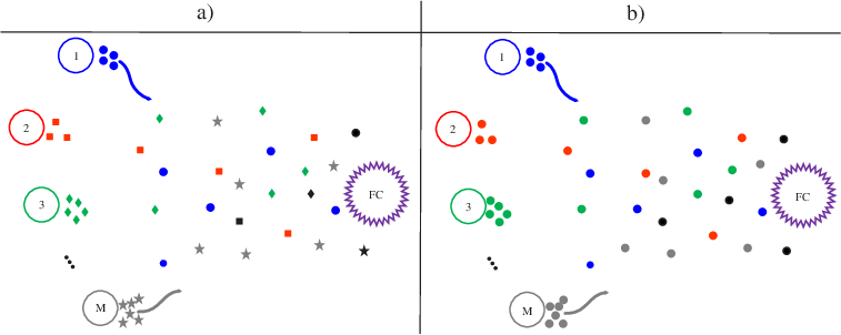
The molecules released by the sensors propagate through the channel and are observed at the FC. We assume that a molecule is absorbed at the FC when it hits the surface of the FC. For simplicity of analysis, we assume that the channels between the sensors and the FC are statistically identical, i.e., the distances between all sensors and the FC are identical. In particular, let $h_{k}$ denote the hitting probability, i.e., the probability that the molecule released in the current time slot hits the receiver during the $k$-th next time slot. The hitting probability $h_{k}$ depends on the communication medium [22]. For instance, for a general three-dimensional environment with a point-source transmitter located at the origin and having a distance of $r_{1}$ from the center of a spherical receiver with radius $r_{2}$, the hitting probability is given by [22]

where $D$ is the diffusion coefficient of the transmitted molecule and $\text{erfc}(x)=\frac{2}{\sqrt{\pi}}\int_{x}^{\infty}\text{e}^{-t^{2}}\text{d}t$ is the complementary error function. For general MC channels, the hitting probabilities $h_{k},\,\,\forall k$, can be estimated using training sequence-based channel estimators [23].

Let $Y_{n}^{\{m\}}$ be a RV which models the number of molecules of the type that the $m$-th sensor employs observed at the FC in the $n$-th time slot and let $y_{n}^{\{m\}}$ be a realization of RV $Y_{n}^{\{m\}}$. Therefore, the $y_{n}^{\{m\}}$, $m\in\{1,\ldots,M\}$, constitute the received signals at the FC for DTM. In contrast, for STM, the FC is not able to distinguish between the molecules released by different sensors as all sensors employ the same type of molecule. In this case, the total number of molecules absorbed at the FC in the $n$-th time slot is modelled by RV $Y_{n}=\sum_{m=1}^{M}Y_{n}^{\{m\}}$. Hereby, we denote a particular realization of RV $Y_{n}$ by $y_{n}$ which constitutes the received signal at the FC. Assuming synchronous transmission [24], the input-output relationships of the channels between the sensors and the FC are modeled as independent Poisson channels with additive Poisson noise [5, 20, 25], i.e.,

where $J_{m}$ and $J$ are the expected numbers of environmental noise molecules observed at the FC in each time slot. We assume that the expected number of noise molecules is identical for all types of signaling molecules employed, i.e., $J_{m}=J,\,\,\forall m$, holds. From (3), we observe that both $Y_{n}^{\{m\}}$ and $Y_{n}$ comprise three independent terms: i) $J$, the noise term, ii) $h_{0}x_{m}A^{\max}$, the expected number of received molecules due to the current transmission, and iii) $\sum_{k=1}^{n}h_{k}x_{m}A^{\max}$, the expected number of received molecules due to previous transmissions.

The term $A_{n}\triangleq\sum_{k=0}^{n}h_{n}A^{\max}$ increases with increasing $n$ and saturates to constant $A\triangleq\sum_{k=0}^{\infty}h_{k}A^{\max}$ for $n\rightarrow\infty$. The speed of convergence depends on the environment, i.e., the values of the $h_{k},\,\,\forall k$. If the channel has a finite memory of $\bar{k}T$, i.e., $h_{k}=0,\,\,\forall k\geq\bar{k}$, the transient effect vanishes after $\bar{k}$ time slots, and then, the expected number of molecules received in each time slot will be constant, i.e., $A_{n}=A,\,\,\forall n>\bar{k}$. The transient period during $0\leq n\leq\bar{k}$, adds a non-uniformity to the hypothesis testing problem. However, for a channel memory $\bar{k}T$ much less than the reporting period of $NT$, the transient period can be neglected. In fact, there are several options for mitigating the effect of the transient period: i) choosing $N\gg\bar{k}$ so that we can neglect the first $\bar{k}$ time slots without compromising the performance, ii) choosing $T$ sufficiently large such that $h_{k}\approx 0,~\forall k\geq 1$, and iii) employing enzymes [26] to speed up the decaying of the channel impulse response (CIR) as a function of time, see [6, Section 2] for further justification. Using either of these approaches, the expected number of molecules received at the FC from a given sensor will be constant in each time slot. Thus, assuming that observations at the FC in different time slots are identically distributed, for DTM, the probability distribution of $(Y^{\{m\}}_{1},\dots,Y^{\{m\}}_{N})$ is given by

where $\mathsf{P}(\cdot)$ denotes probability. Eq. (4) also holds for STM after removing superscript $\{m\}$.

The FC is assumed to be a node with sufficient processing capability that is able to make decisions based on the molecules received from the sensors. A promising approach for implementing such a node is using engineered bacteria [27] where the bacteria can be designed to individually detect and count different types of molecules. Such engineered bacteria may also be able to perform simple processing tasks. To perform more sophisticated processing, one approach is to employ a synthetic/electronic nano-machine with sufficient processing capability to aid the engineered bacteria. Alternatively, for applications where a nano-machine only collects observations and forwards them to an external processing unit which serves as the FC outside the MC environment, high computational complexity may be affordable. This case may apply e.g. in health monitoring when a computer outside the body may be available for offline processing [23].

To calculate the LLR in (7), we have to first derive the conditional distributions of the received molecules at the FC, i.e., $\mathsf{P}\left(\vec{Y}=\vec{y}|\mathcal{H}_{i}\right),\,\,i=0,1$. In particular, we have

where $\vec{Y}^{\{m\}}=[Y_{1}^{\{m\}},\dots,Y_{N}^{\{m\}}]^{T}$ denotes an RV modelling the DTM observation originating from sensor $m$ at the FC, i.e., the numbers of the molecules received from the $m$-th sensor in the $N$ time slots of the reporting period, and $\vec{y}^{\{m\}}=[y_{1}^{\{m\}},\dots,y_{N}^{\{m\}}]^{T}$ denotes a particular realization of $\vec{Y}^{\{m\}}$. Moreover, for $i=0,1$ and $m=1,\ldots,M$, $\mathsf{P}\left(\vec{Y}^{\{m\}}|\mathcal{H}_{i}\right)$ is obtained as

where equality $(a)$ follows from the fact that the observations in different time slots, i.e., $Y_{n}^{\{m\}},\,\,\forall n$, are independent, and equality $(b)$ is obtained by substituting $\mathsf{P}\big(\vec{Y}^{\{m\}}=\vec{y}^{\{m\}}|X^{\{m\}}=\\ x_{m},\mathcal{H}_{i}\big)$ by the Poisson distribution with mean $x_{m}A+J$. Since the sensors are assumed to be independent, the total LLR is the sum of the LLRs of all sensors [11], i.e., we have

where

For the special case of $L=2$, i.e., hard decisions at the sensors, the total LLR can be simplified to

Using (10), the optimal decision can be obtained from (III).

The following theorem reveals the monotonicity of $\mathsf{LLR}(\vec{y}^{\{m\}})$ with respect to $\sigma_{y}^{\{m\}}=\sum_{n=1}^{N}y^{\{m\}}_{n}$ under some mild conditions. In Section IV, we exploit this property to present a low-complexity two-stage detector for DTM.

Assuming the probability functions $\text{g}_{0}(x_{m})$ and $\text{g}_{1}(x_{m})$ are decreasing and increasing functions of $x_{m}$, respectively, the condition in Theorem 1 always holds. In fact, it is expected that $\text{g}_{0}(x)$ and $\text{g}_{1}(x)$ have the aforementioned properties for practical sensors. For instance, under hypothesis $\mathcal{H}_{1}$, a sensor with a reasonable performance would be expected to yield $\text{g}_{1}(x)>\text{g}_{1}(x^{\prime})$ for $x>x^{\prime}$.

In this subsection, we focus on sensors employing STM reporting, i.e., all sensors employ the same type of molecule for signaling their observations to the FC. Therefore, the FC cannot distinguish between the molecules released by different sensors. In this case, the conditional probability distribution of the received molecules at the FC can be written as

where $X=\sum_{m=1}^{M}X^{\{m\}}$ is the sum of all sensing values. The possible values, $x$, of $X$, lie in the set $\mathcal{X}^{\prime}\triangleq\{l/(L-1):l=0,1,\cdots,M(L-1)\}$, i.e., $x\in\mathcal{X}^{\prime}$. The probability $\mathsf{P}\left(\vec{Y}=\vec{y}\big|X=x,\mathcal{H}_{i}\right)$ is obtained as

where for equality $(a)$, we exploit the mutual independence of the observations, $Y_{n},\,\,\forall n$, and for equality $(b)$, the expression for the Poisson distribution with mean $xA+J$ is substituted for $\mathsf{P}\big(Y_{n}=y_{n}\big|X=x,\mathcal{H}_{i}\big)$. The probability $\mathsf{P}\left(X=x|\mathcal{H}_{i}\right)$ can be calculated as

where “$\otimes$” represents the convolution operator. Using (16) and (17), we can rewrite (15) as

Therefore, the LLR for STM can be calculated as

Having the LLR in (19), the optimal decision can be readily obtained from (III). In the following corollary, we prove the monotonicity of the above LLR function in $\sum_{n=1}^{N}y_{n}^{\{m\}}$. Then, based on this property, we propose a low-complexity optimal detector.

Based on Corollary 1, $\overline{\mathsf{LLR}}(\vec{y})$ is strictly increasing in terms of $\sum_{n=1}^{N}y_{n}$. Let us denote this mapping by $\overline{\mathsf{LLR}}(\vec{y})=f(\sum_{n=1}^{N}y_{n})$ and its inverse by $f^{-1}(\overline{\mathsf{LLR}}(\vec{y}))=\sum_{n=1}^{N}y_{n}$. Therefore, comparing $\overline{\mathsf{LLR}}(\vec{y})$ with threshold $\gamma$, cf. (III), is equivalent to comparing $\sum_{n=1}^{N}y_{n}$ with a new threshold $\gamma_{\text{STM}}=f^{-1}(\gamma)$. This leads to the following equivalent optimal detector

We note that the above detector is much simpler than that in (III) since the computation of the LLR in (19) is avoided.

This approximation, first introduced in [28] for classical wireless sensor networks, takes into account only the maximum terms in both the numerator and denominator of $\mathsf{LLR}_{\text{opt}}$ in (22). That is,

Since the $\mathsf{log}(\cdot)$ function is monotonically increasing, we have $\max_{x}f(x)=\mathsf{exp}(\max_{x}\mathsf{log}(f(x)))$. Applying this rule to (23), we obtain

As can be seen from (24), unlike the optimal $\mathsf{LLR}_{\text{opt}}\left(\sigma_{y}^{\{m\}}\right)$ in (22), the expression for the sub-optimal $\mathsf{LLR}_{\text{Max-Log}}\left(\sigma_{y}^{\{m\}}\right)$ is a linear function of $\sigma_{y}^{\{m\}}$ which facilitates its numerical evaluation. The sub-optimal detector for the max-log approximation is obtained from (III) by substituting $\mathsf{LLR}_{\text{Max-Log}}$ for $\mathsf{LLR}\left(\vec{y}^{\{m\}}\right)$ in (10).

For the MRC approximation [29], all sensors are assumed to be ideal, i.e., $\text{g}_{0}(x_{m})=\delta(x_{m})$ and $\text{g}_{1}(x_{m})=\delta(x_{m}-1)$. By substituting the ideal sensing distributions into (22), we obtain

The sub-optimal $\mathsf{LLR}_{\text{MRC}}\left(\sigma_{y}^{\{m\}}\right)$ is in fact a linear function in $\sigma_{y}^{\{m\}}$ which again facilitates its numerical evaluation. In addition, applying the MRC approximation given in (25) in (III), the detector essentially compares the summation of all molecules received from all sensors in all time slots with a suitable threshold, denoted by $\gamma_{\text{MRC}}$. This leads to the following simple detector

The MRC detector is expected to perform well when the sensors are reliable but the reporting channel is unreliable.

For the CV approximation, which was first introduced in [30] for classical sensor networks, instead of substituting the numerator and denominator of the LLR in (22) with their corresponding maximum terms as in the Max-Log decision rule, we first find the value of $x_{m}$ in (22) that maximizes only the Poisson terms in the numerator and denominator denoted by $\hat{x}_{m}$. This leads to

where for equality $(a)$, we exploited that the $\mathsf{log}(\cdot)$ function is monotonically increasing. Then, the LLR is approximated as

By substituting the above approximated LLR into (10), the corresponding sub-optimal detector is given by (III). The CV detector is expected to perform well in situations where the reporting channel is reliable but the sensors are unreliable.

In this part, we consider a simple sub-optimum detector, where the decision is made in two stages. In the first stage, the FC makes a separate decision on the observations received from each sensor. Then, in the second stage, the global final decision is made using the $M$ individual decisions. Our motivation for considering this sub-optimum detector is that it is simple and it may be more practical when the adopted FC is a biological entity. In particular, for some biological cells, the processing unit of a cell does not have direct access to the counted molecules. Rather, a preliminary decision may be made by the signaling pathway which connects the receptors to the processing unit of the cell [2].

For each sensor $m$, the detector makes a local decision by comparing $\mathsf{LLR}(\vec{y}^{\{m\}})$, given in (11), with threshold level $\tau$, that is

Using Theorem 1, the optimum local decision rule in (IV-D) can be further simplified for ease of implementation. In particular, in Theorem 1, we showed that $\mathsf{LLR}(\vec{y}^{\{m\}})$ is strictly increasing in terms of $\sum_{n=1}^{N}y^{\{m\}}_{n}$. That is, $\mathsf{LLR}(\vec{y}^{\{m\}})$ is a monotonic function in $\sum_{n=1}^{N}y^{\{m\}}_{n}$. This property implies that, comparing $\sum_{n=1}^{N}y^{\{m\}}_{n}$ with an appropriate new threshold, denoted by $\gamma_{\text{local}}$, is equivalent to comparing the LLR, $\mathsf{LLR}(\vec{y}^{\{m\}})$, with the original threshold, $\tau$. Therefore, the optimal local decision can be simplified to

In the second stage, the detector makes the final decision based on the number of sensors that have made a local decision in favor of $\mathcal{H}_{1}$. If the number of sensors with $\text{d}_{\text{local}}^{\{m\}}=1$ is larger than a new threshold, $\gamma_{\text{global}}$, the final decision is $\mathcal{H}_{1}$, otherwise it is $\mathcal{H}_{0}$. This leads to

We note that the above two-stage detector has been also considered in the context of spectrum sensing in cognitive radio networks and is there referred to as “hard decision” with “$K$-out-of-$M$” decision rule where $K=\gamma_{\text{global}}-1$ [31]. Special cases of the $K$-out-of-$M$ decision rule are the “OR” rule where $K=1$ and the “AND” rule where $K=M$.

The proposed sub-optimal LLRs for DTM are computationally much simpler compared to the optimal LLR. However, it is expected that this simplicity is accompanied by a loss in performance. Hence, in the following, we study the accuracy of the proposed LLR approximations for a simple example. Fig. 2 shows $\mathsf{LLR}_{\text{opt}}\left(\sigma_{y}^{\{m\}}\right)$ and its approximations, namely $\mathsf{LLR}_{\text{Max-Log}}\left(\sigma_{y}^{\{m\}}\right)$, $\mathsf{LLR}_{\text{MRC}}\left(\sigma_{y}^{\{m\}}\right)$, and $\mathsf{LLR}_{\text{CV}}\left(\sigma_{y}^{\{m\}}\right)$, versus $\sigma_{y}^{\{m\}}=\sum_{n=1}^{N}y_{n}^{\{m\}}$ for $L=4$, $J=4$, $N=10$, and $A=6$. While the optimum LLR is generally non-linear, all approximated LLRs are piecewise linear. Among the different approximations, the Max-Log approximation follows the optimum LLR most closely. Thus, we expect that the Max-Log detector outperforms the other proposed sub-optimal detectors. More detailed discussions regarding the relative performance of the proposed detectors are provided in Section VI.

For STM, we can adopt $\sigma_{y}=\sum_{m=1}^{M}\sum_{n=1}^{N}y_{n}^{\{m\}}$ as the decision variable instead of the LLR, see Corollary 1 and (21). This facilitates the derivation of closed-form expressions for the false alarm and detection probabilities. In particular, the false alarm probability can be derived as

References

- [1] T. Nakano, A. Eckford, and T. Haraguchi Molecular communication. Cambridge Univ. Press, Cambridge, U.K., 2013.
- [2] B. Alberts, D. Bray, K. Hopkin, A. Johnson, J. Lewis, M. Raff, K. Roberts, and P. Walter, Essential Cell Biology. Garland Science, 4th ed., 2014.
- [3] I. F. Akyildiz, J. M. Jornet, and M. Pierobon, “Nanonetworks: A new frontier in communications,” Commun. of the ACM, vol. 54, no. 11, pp. 84-89, 2011.
- [4] M. Kuran, H. Yilmaz, T. Tugcu, and I. Akyildiz, “Modulation techniques for communication via diffusion in nanonetworks,” in Proc. IEEE Int. Conf. Commun. (ICC), pp. 1-5, Jun. 2011.
- [5] R. Mosayebi, H. Arjmandi, A. Gohari, M. Nasiri-Kenari, and U. Mitra, “Receivers for diffusion-based molecular communication: exploiting memory and sampling rate,” IEEE J. Select. Areas in Commun., vol. 32, no. 12, pp. 2368-2380, Dec. 2014.
- [6] V. Jamali, N. Farsad, R. Schober, and A. Goldsmith, “Non-coherent multiple-symbol detection for diffusive molecular communications,” in Proc. ACM Int. Conf. Nanoscale Comput. Commun. (Nanocom), Sept. 2016.
- [7] A. Ahmadzadeh, H. Arjmandi, A. Burkovski, and R. Schober, “Comprehensive reactive receiver modeling for diffusive molecular communication systems: reversible binding, molecule degradation, and finite number of receptors,” IEEE Trans. Nanobiosci., vol. 15, no. 7, pp. 713-727, Oct. 2016.
- [8] B. Atakan, O. B. Akan, “On molecular multiple-access, broadcast, and relay channels in nanonetworks,” in Proc. Int. Conf. Bio-Inspired Models Netw., Inf. Comput. Sys. (BIONETICS), Nov. 2008.
- [9] T. Nakano, J. Moore, F. Wei, V. Vasilakos, and Jianwei Shuai, “Molecular communication and networking: Opportunities and challenges,” IEEE Trans. Nanobiosci., vol. 11, no. 2, pp. 135-148, June 2012.
- [10] U. A. K. Chude-Okonkwo, R. Malekian, and B. T. S. Maharaj, “Molecular communication model for targeted drug delivery in multiple disease sites with diversely expressed enzymes,” IEEE Trans. Nanobiosci., vol. 15, no. 3, pp. 230-245, Apr. 2016.
- [11] H. V. Poor, An introduction to signal detection and estimation theory, Springer Verlag, New York, 1994.
- [12] V. Chandola, A. Baaerjee and V. Kumar, “Anomaly detection : A survey,” ACM Computing Surveys, Sept. 2009.
- [13] V. V. Phoha, The springer internet security dictionary. Springer Verlag, 2002.
- [14] T. Fawcett, and F. Provost, “Activity monitoring: Noticing interesting changes in behavior,” in Proc. ACM SIGKDD Int. Conf. Knowledge Discovery, Data Mining, pp. 53-62, Aug. 1999.
- [15] M. Basseville and I. V. Nikiforov, Detection of abrupt changes - Theory and application, Prentice-Hall, Inc., 1998.
- [16] K. Cichoń, A. Kliks and H. Bogucka, “Energy-efficient cooperative spectrum sensing: A survey,” IEEE Commun. Surveys & Tutorials, vol. 18, no. 3, pp. 1861-1886, 2016.
- [17] V. Jamali, N. Reisi, M. Ahmadian, and S. Salari “Optimization of Linear Cooperation in Spectrum Sensing Over Correlated Log-normal Shadow Fading Channels,” Wireless Personal Commun., Springer, vol. 73, no. 3, pp. 1691-1706, 2013.
- [18] Y. Fang, A. Noel, N. Yang, A. W. Eckford, and R. A. Kennedy, “Distributed cooperative detection for multi-receiver molecular communication,” in Proc. IEEE Global Commun. Conf. (Globecom), pp. 1-7, Dec. 2016.
- [19] S. Ghavami and F. Lahouti, “Abnormality detection in correlated Gaussian molecular nano-networks: design and analysis,” IEEE Trans. NanoBiosci., 2017.
- [20] H. B. Yilmaz and C. B. Chae, “Arrival modelling for molecular communication via diffusion,” Electron. Lett., vol. 50, no. 23, pp. 1667–1669, 2014.
- [21] H. Arjmandi, A. Gohari, M. Nasiri-Kenari and Farshid Bateni, “Diffusion based nanonetworking: A new modulation technique and performance analysis,” IEEE Commun. Lett., vol. 17, no. 4, pp. 645-648, Apr. 2013.
- [22] H. B. Yilmaz, A. C. Heren, T. Tugcu, and C.-B. Chae, “Three dimensional channel characteristics for molecular communications with an absorbing receiver,” IEEE Commun. Lett., vol. 18, no. 6, pp. 929-932, Jun. 2014.
- [23] V. Jamali, A. Ahmadzadeh, C. Jardin, C. Sticht, and R. Schober, “Channel estimation for diffusive molecular communications,” IEEE Trans. Commun., vol. 64, no. 10, pp. 4238–4252, Oct. 2016.
- [24] V. Jamali, A. Ahmadzadeh and R. Schober, “Symbol synchronization for diffusive molecular communication systems,” accepted for presentation at IEEE Int. Conf. Commun. (ICC) 2017, available online on arXiv: 1610.09141.
- [25] R. Mosayebi, H. Arjmandi, A. Gohari, M. Nasiri-Kenari, and U. Mitra, “Diffusion based molecular communication: A simple near optimal receiver,” in Proc. IEEE Iran Workshop Commun. Inf. Theory (IWCIT), pp. 1-4, May 2014.
- [26] A. Noel, K. Cheung, and R. Schober, “Improving receiver performance of diffusive molecular communication with enzymes,” IEEE Trans. NanoBiosci., vol. 13, no. 1, pp. 31–43, Mar. 2014.
- [27] M. Wells, M. Gosch, R. Rigler, H. Harms, T. Lasser, and J. Roelof van der Meer, “Ultrasensitive reporter protein detection in genetically engineered bacteria,” Analytical Chemistry, no. 77, vol. 9, pp. 2683-2689, May 2005.
- [28] A. Lei and R. Schober, “Coherent max–log decision fusion in wireless sensor networks” IEEE Trans. Commun., vol. 58, no. 5, May 2010.
- [29] R. Niu, B. Chen, and P. K. Varshney, “Fusion of decisions transmitted over Rayleigh fading channels in wireless sensor networks,” IEEE Trans. Sig. Process., vol. 54, pp. 1018–1027, Mar. 2006.
- [30] B. Chen, R. Jiang, T. Kasetkasem, and R. K. Varshney, “Channel aware decision fusion in wireless sensor networks,” IEEE Trans. Sig. Process., vol. 52, pp. 3454–3458, Dec. 2004.
- [31] K. Cichon, A. Kliks, and H. Bogucka, “Energy-efficient cooperative spectrum sensing: A survey,” in IEEE Commun. Surveys & Tutorials, vol. 18, no. 3, pp. 1861-1886, third quarter 2016.
- [32] J. A. Bucklew and J.S. Sadowsky, “A contribution to the theory of Chernoff bounds,” IEEE Trans. Inf. Theory, vol. 39, no. 1, pp. 249-254, Jan. 1993.