Modular Bayes screening for high-dimensional predictors
Yuhan Chen
Affiliation: Department of Statistical Science
Affiliation: Duke University, Durham, NC 27708
Affiliation: email: yuhan.chen@duke.eduDavid Dunson
Affiliation: Department of Statistical Science
Affiliation: Duke University, Durham, NC 27708
Affiliation: email: dunson@duke.edu
Abstract
With the routine collection of massive-dimensional predictors in many application areas, screening methods that rapidly identify a small subset of promising predictors have become commonplace. We propose a new MOdular Bayes Screening (MOBS) approach, which involves several novel characteristics that can potentially lead to improved performance. MOBS first applies a Bayesian mixture model to the marginal distribution of the response, obtaining posterior samples of mixture weights, cluster-specific parameters, and cluster allocations for each subject. Hypothesis tests are then introduced, corresponding to whether or not to include a given predictor, with posterior probabilities for each hypothesis available analytically conditionally on unknowns sampled in the first stage and tuning parameters controlling borrowing of information across tests. By marginalizing over the first stage posterior samples, we avoid under-estimation of uncertainty typical of two-stage methods. We greatly simplify the model specification and reduce computational complexity by using modularization. We provide basic theoretical support for this approach, and illustrate excellent performance relative to competitors in simulation studies and the ability to capture complex shifts beyond simple differences in means. The method is illustrated with applications to genomics by using a very high-dimensional cis-eQTL dataset with roughly 38 million SNPs.
Keywords: Genomics; High-dimensional; Independent screening; Large p small n; Mixture model; Modularization; Nonparametric Bayes; Variable selection.
1 Introduction
In modern scientific research, it has become routine to collect massive dimensional data for each study subject, leading to a massive small to moderate statistical problem. In most scientific studies collecting high-dimensional data, the over-arching interest is not in developing a black-box model for prediction; instead the focus is on variable selection. In particular, the scientists would like to select the subset of features out of a high-dimensional set of candidates , which are predictive of a response , with indexing the subject under study. There is a vast recent literature on high-dimensional feature/variable selection, with the overwhelming focus on one of two strategies. The first is to use a penalized optimization method, such as Lasso (Tibshirani 1996), SCAD (Fan and Li 2001), Dantzig selector (Candes and Tao 2007) or other variants, to obtain a sparse estimate of the regression coefficient vector. In general, such an approach has adequate performance only when the feature matrix satisfies a number of stringent conditions, which seldom hold in scientific applications even approximately. When these assumptions are violated, performance can degrade badly.
This fact has lead to an emphasis on the second strategy, which is to first apply an independent screening algorithm using measures of association between and separately for , and then select features based on thresholding the corresponding p-values, test statistics or association estimates to maintain a superset containing most of the important features along with a number of false positives. This strategy was proposed by Fan and Lv (2008) using marginal correlation for sure independence screening (SIS). Fan and Song (2010) extended the idea to generalized linear models and Fan et al. (2011) considered nonparametric additive models. Zhu et al. (2011) introduced model-free screening via sure independent ranking and screening (SIRS). Other model-free procedures include the distance correlation screening (DCS) in Li et al. (2012) and the fused Kolmogorov filter in Mai and Zou (2013) and Mai and Zou (2015).
The focus of this article is on improving upon high-dimensional screening methodology through using Bayesian nonparametric and hierarchical models to avoid parametric assumptions on the data generating model, while borrowing information across the many tests being conducted. A potentially key disadvantage of most existing screening methods is the lack of any borrowing of information across the different tests. A novel idea we propose, which should have impact beyond the screening case, is to place a nonparametric Bayes model on the marginal distribution of the response, with inclusion tests for each predictor then defined conditionally on unknowns in the marginal distribution. This approach has the dual advantages of avoiding parametric assumptions on the distribution of the response, while also automatically borrowing information across the screening tests through their shared conditioning on a common set of unknowns. In addition to this novel type of borrowing, we additionally place a more convention Bayesian hierarchical structure on the probability of variable inclusion, related to Scott and Berger (2010). A key advantage of the proposed formulation is that we can characterize uncertainty in posterior computation for the marginal response distribution via integrating conditional posterior probabilities of variable inclusion across first stage posterior samples. This is computationally scalable and avoids the under-estimation of uncertainty typical of two-stage procedures..
One caveat about our proposed approach is that it is not a coherent fully Bayes probability model in that we ignore certain dependencies for simplicity, robustness and computational tractability. In particular, to define a fully Bayes model for the marginal distribution of the response in settings involving predictors , we would require a model for the conditional distribution of the response given all the predictors along with a model for the joint distribution of the predictors . In very large settings, computational and complexity considerations force a focus on relatively simple settings involving strong constraints (e.g., Gaussian, linear, highly sparse, etc). In most settings, such constraints are inconsistent with available prior information, and results are therefore highly questionable. Instead, we take the more mild approach of ignoring information on in defining the marginal distribution of . This is a type of modularization (Liu et al. 2009). The idea of modularization is that Bayesian models can be defined in modules, with posterior computation in certain modules not taking into account the model structure and data in other modules. In our case, the model for the marginal density is one module, and we do not attempt to take into account information about the predictors in fitting this module. We suspect that closely related ideas may be a game changer in making (approximately) Bayesian approaches practical in modern massive dimensional data settings.
The existing literature on nonparametric Bayes variable selection is sparse. There are several methods for two group comparisons (Dunson and Peddada 2008; Ma and Wong 2011; Holmes et al. 2015), but such methods are computationally intensive for each group, and would need to be applied separately times. There are also several approaches that are designed for variable selection in Bayesian nonparametric models for conditional response distributions, . For example, Chung and Dunson (2009) proposed a stochastic search variable selection algorithm under a probit stick-breaking mixture model for . Kessler et al. (2014) and Yang and Dunson (2016) used tensor factorizations to characterize the conditional distribution in order to capture complex interactions between the predictors. Jiang et al. (2017) introduced a nonparametric test using a nonparametric Bayesian slice inversed regression based on modeling the conditional distribution of a covariate given the discretized response. Their method is less computationally intensive than previous attempts, but is restricted to univariate . Finally, Filippi et al. (2016) tested for pairwise dependence between two variables using Dirichlet process mixtures, improving efficiency by running MCMC for each marginal in parallel.
In Section 2 we propose the general MOdular Bayes Screening (MOBS) framework, provide basic theoretical support, and sketch a general approach to computation. In Section 3 we focus on the case in which the response is continuous and univariate, motivating a location-scale mixture of Gaussians for the marginal distribution. Section 4 contains a simulation study assessing operating characteristics relative to a variety of high-dimensional screening methods. Section 5 applies the screening method to a massive-dimensional cis-eQTL dataset with approximately 38 million SNPs. Section 6 contains a discussion. Technical details are included in an Appendix.
2 Modular Bayes screening framework
2.1 General framework
MOdular Bayes Screening (MOBS) uses a two stage set-up and starts with a mixture model for the marginal density of the response. For subjects , let denote the response, which can be either univariate or multivariate. Let denote a high-dimensional vector of categorical predictors for subject , with having levels. Suppose that marginally we have independently for ; we refer to as the baseline density. Treating this baseline density as unknown, we apply a finite over-fitted mixture model (Rousseau and Mengersen 2011):
(1)
where is the kernel density, are the weights, the kernel parameters, is the prior distribution for each and is a conservative upper bound on the number of mixture components needed to produce an accurate approximation of the unknown density. Let denote a latent variable vector with being the cluster membership of and . As increases, (1) converges weakly to a Dirichlet process mixture model. This represents a common approximation to the Dirichlet Process mixture model (Ishwaran and Zarepour 2002) facilitating practical implementation.
To generalize the baseline density to allow dependence on the th predictor , we let
(2)
where and , , represent the weights and component parameters for subjects with . Expression (2) modifies the baseline density (1) to allow the weights and kernel parameters to vary with . Let
(3)
correspond to discarding and including the th predictor, respectively. The alternative hypothesis is composed of three cases: , where varies but remains the same, , where varies but is the same and , where both vary. By testing both the weights and the cluster parameters, MOBS is able to capture deeper and more complex shifts in distribution than traditional methods that focus primarily on the mean. Clearly, . Let be the prior probabilities of the four subhypotheses, where is the prior probability of and are the prior probabilities of the alternative hypotheses respectively.
We suppose that the weight and component parameter vectors specific to each level of each predictor are distributed randomly about their baseline values according to the hierarchical model:
(4)
where is a distribution centered on with scale parameter and is the Dirichlet precision controlling variability about the mean . Using a Dirichlet prior for maintains conjugacy with the Multinomial distribution of the component memberships and facilitates marginalizing out when calculating the likelihood. For the same reason, should ideally be conjugate to the kernel density . The precisions control how much changes with predictor for each such that holds. The hierarchical structure favors borrowing of information in learning across different predictors and levels of .
2.2 Algorithmic details
Using (3) allows direct calculation of an analytic form for , where denotes , the baseline weights and component parameters, and denotes , the hyperparameters controlling borrowing of information and multiplicity adjustment in hypothesis testing. The key idea in our proposed MOBS approach is to run MCMC for posterior computation only for the baseline nonparametric model for the marginal response density . We do not know the exact kernel memberships, weights or parameters, and there does not exist a tractable, analytic form for , so MOBS instead takes the Monte Carlo integration of over the samples of generated from the posterior distribution under the baseline model.
Let and be the likelihood conditional on the baseline MCMC output and hyperparameters controlling borrowing of information and multiplicity adjustment in hypothesis testing for and , respectively. Then, we have
where is the conditional likelihood for for . The posterior probabilities of and conditional on the baseline weights and parameters are then, respectively,
(5)
(6)
where for ,
is the Bayes factor in favor of over conditional on the hyperparameters and the baseline weights and parameters.
We calculate the conditional likelihoods given the baseline unknowns and hyperparameters as follows. First, under , we have the simple form:
where , with the number of subjects having and belonging to cluster , and the total number of subjects allocated to each component. For the three alternative subhypotheses
These results imply after some calculations that
Here, provides a weight of evidence of changes in mixture weights with , while provides the same for different kernels. provides evidence for both weights and kernels being different and interestingly ends up being the product of and .
Algorithm 1 Modular Bayes Screening
1:Inputs:
2:data
3:Initialize:
4:
5:
Obtain samples for from the posterior distribution under baseline mixture model using MCMC or an alternative algorithm.
6:repeat
7:
Estimate and for by averaging and , respectively, over the baseline samples for each .
8:
Set using the average of the , , , and estimated above, respectively.
9:until convergence
We initialize , . Estimating involves iteratively taking the average of the posterior probabilities for each subhypothesis, which is effectively an empirical Bayes procedure. Our proposed MOBS approach leverages on the simplicity of posterior computation for and the simple analytic forms shown above via Algorithm 1.
3 Univariate continuous response
3.1 Computation
While the proposed method allows for complex, arbitrary responses, this section provides an example under a simple univariate, continuous setting. The baseline density is represented as a mixture of univariate location-scale Gaussian kernels:
(7)
where are the mean and variance parameters of the component with prior . Details on the Gibbs sampler for the base distribution can be found in the Appendix. The conditional density can similarly be represented as
(8)
where with prior with , and the scale parameters .
To derive , note that for each and ,
where is the multivariate beta function. Hence
(9)
Similarly to find for each , first note that
and
where
It follows that
(10)
Running MOBS requires first generating samples of and from the posterior under the baseline mixture model. One then iteratively alternates between estimation of using (9) and (10) over the samples of the baseline and and estimation of as the average of the estimated posterior probabilities. The strength of MOBS lies in the ease of computing and in a trivially parallelizable manner. The overall algorithm has computational complexity . The approach can be trivially modified to accommodate multivariate and discrete settings; in such cases, expression (10) will take a different form.
3.2 Hyperparameters selection
An important question when running MOBS is the selection of hyperparameters, especially that of the precision parameters . The various can be interpreted as the precisions controlling the distance between the density of under the null hypothesis and that of under the alternative hypothesis. Naturally, higher values of would suggest a smaller distance, as converges to when .
We aim to tune such that the prior signal-to-noise ratio is within a reasonable range somewhere between and . For any fixed and , let . Given , the densities of and are
Let
be the average square of -norm distances between the densities of and and between those of and respectively. Since , we know
While and are both intractable, we can estimate their values by averaging and over samples of . Empirically, we find that for a given , setting provides a reasonable default specification that is relatively stable and has a signal-to-noise ratio between 0.05 and 0.1.
3.3 Theoretical properties
We initially study asymptotic properties of MOBS treating parameters as known, and then consider sure screening consistency under general settings. We first investigate properties of . The posterior odds conditioned on and are
Set . For , and , let
Therefore, and where . Let and be the true values of and , respectively, for . Then under , , and .
Theorem 3.1
Let , with for some fixed . Treat as known.
(1) When is true, we have with rate and
with rate . These two estimates imply that with rate .
(2) Under the condition , we have with rate and under the condition , we have with rate where
Therefore under , with rate .
The above theorem shows rates of convergence of hypothesis probabilities and Bayes factors for the different hypotheses in the event that the true weights, parameters and cluster allocations are known. However, in practice MOBS uses posterior samples for the baseline parameters to account for uncertainty. Now consider the situation where the parameters are unknown and the model may be misspecified. In particular, we extend our above results using misspecification techniques given in Kleijn and van der Vaart (2006) and used in Lock and Dunson (2015). Let be the set of all convex combinations of Gaussian distributions where and let define a prior on . Let be the true distribution and the closest convex combination in to under Kullback-Leibler divergence. We define to be a neighborhood of the density under the measure induced by the density :
and define to be the weighted Hellinger distance
Lemma 3.2
Let be independent with density . Assume exists and for all where is the posterior measure given prior . Let be the component weights and be the kernel parameters corresponding to and let and be the true weights and kernel parameters. Assume and are unique in that only if . Then for any fixed ,
Theorem 3.3
For , let denote the subset of with size such that . Assume are independent with density and are independent with density . Let
Assume the uniqueness condition for the previous theorem holds for and . If , as and if , as .
This result suggests that our posterior probability is consistent under and holds under weak conditions under for each . However, consistency can fail under when and have the same closest point under K-L divergence in . In practice, and would need to be extremely close to have the same closest point, so this is a very mild condition.
Next, we use the previous theorem to establish sure screening consistency for MOBS. Following standard screening conventions (Li et al. 2012), let denote the conditional distribution function of given the predictors . Define
to be the true set of relevant predictors. A good screening method can identify a small subset such that . Existing literature have focused predominantly on frequentist methods that select based on rankings or thresholding using some test statistic such as marginal correlation in SIS or distance correlation in DCS. MOBS instead relies on thresholding of the estimated posterior null probabilities for . In particular, let
where are the order values and is an integer. Let if the th predictor is marginally related to and otherwise. We impose the following two conditions:
(C1) All jointly important predictors are also marginally important (i.e. ) and .
(C2) All jointly important predictors satisfy the constraint that and are not the closest in K-L divergence to the same .
Condition 1 is similar to conditions found in the screening literature (Fan and Lv 2008), restricting metrics of marginal importance for important predictors to be non-zero. Condition 2 requires Theorem 3.3 to be satisfied, and is mild as noted above.
Theorem 3.4
Under conditions (C1) and (C2), when ,
4 Simulation
4.1 Screening accuracy
In this section, we assess the performance of MOBS against five existing screening methods using simulated datasets. The first competitor is sure independence screening or SIS (Fan and Lv 2008), and we use the SISR package. We also compare against three frequentist model-free methods, sure independent ranking and screening or SIRS (Zhu et al. 2011), using code found at
http://users.stat.umn.edu/ wangx346/research/example1b.txt, the distance correlation screening or DCS (Li et al. 2012), using the energyR package and the fused Kolmogorov filter (Mai and Zou 2015) using code provided by the authors. Finally, we compare to the JYL Bayesian nonparametric test (Jiang et al. 2017) with code found at http://www.people.fas.harvard.edu/ junliu/BF/bfslice.html.
We simulate 100 replicates for all methods under six different models. Under these settings, we test observations and total predictors and generate and . First, we consider the case where is independent and generate the features with , , for all 2000 predictors. However, in biological applications (e.g. involving SNPs), can often exhibit moderate correlations in blocks of predictors. To mimic such settings, we randomly select 600 predictors and draw them in the following fashion with correlation . We first draw for each for and . Next, construct by replacing the first rows of such that for for some constant ,
To convert this continuous data to multinomial, for each predictor, we can simply assign them by quantiles. The remaining 1900 predictors are generated from independent Gaussians without correlation.
, where is independent of and is uncorrelated.
is generated the same as with Model 1 but with a block of predictors with correlation described above.
, where is independent of and is uncorrelated.
is generated the same as with Model 3 but with a block of predictors with correlation described above.
is generated using 6 predictors at positions chosen at random from . Let be the true vector of jointly important indices. The resulting marginal density is then sampled from mixtures of Gaussian distributions with mean and standard deviation each corresponding to different permutations of . If , we subsequently draw . is generated to be uncorrelated.
is generated the same as with Model 5 but with a block of predictors with correlation described above.
In order to implement MOBS, we use the computational strategy described in Section 2 and Section 3 and set the deafult hyperparameters , with for the linear case since we expect the response to be mostly unimodal and for the more multimodal single index and mixture models. We run the Markov chain of the baseline model 6000 times and perform Monte Carlo integration using the last 500 samples. If potential issues involving label-switching for the samples of arise, we use methods found in Stephens (2000) and Papastamoulis (2016).
Figure 1: ROC curves for all six methods under linear, single index and mixture settings, both correlated and uncorrelated.
Figure 1 summarizes the ROC curves for the six different methods by comparing the true positive rate against the false positive rate. In each of the simulations, MOBS exhibits the best or one of the best performance in comparison to the SIS, SIRS, DCS, the fused Kolmogorov filter and the JYL approaches. In the mixture setting, the nonparametric methods dominate as expected. For the linear regression case and single index case, the other two nonparametric methods, the fused Kolmogorov filter and JYL both demonstrate weakness in these settings, but MOBS still performs strongly and is comparable to SIS. In a multimodal mixture setting, both and play large roles in detecting change, whereas in a unimodal setting, is less relevant and MOBS reduces to essentially a -test.
4.2 Computational efficiency
Understanding the computational efficiency of variable screening is important as the various methods should be scalable to huge data sets. We measure the total time taken to run each of the six methods under two different settings using data generated from an uncorrelated linear regression model setting in Model 1 but with varying and . Our first example fixes the number of subjects at 250 and then alter the number of predictors. Next, we fix the number of predictors at 2500 and instead change the number of subjects.
Figure 2: Computational speed against number of samples when and computational speed against number of predictors when .
Figure 2 summarize the results under both methods. As expected, the linear predictor SIS exhibits significantly faster performance as a simple parametric model though MOBS remains competitive against the other nonparametric and model-free screening methods. All six screening methods are simple to parallelize and scale linearly with the number of predictors . However, in regards to the number of samples , MOBS scales linearly unlike slower competitors such as JYL and DCS.
5 Applications
5.1 Data
Figure 3: Histogram of (Ensemble ID: ENSG00000007968) with the estimated density from sampling the baseline model with clusters.
In this section, we illustrate our approach by analyzing the GEUVADIS cis-eQTL dataset (Lappalainen et al. 2013), publicly available at http://www.ebi.ac.uk/Tools/geuvadis-das/. The data set consists of messenger RNA and microRNA on lymphoblastoid cell line (LCL) samples from 462 individuals provided by the 1000 Genomes Project along with roughly 38 million SNPs. These individuals are taken from 5 different populations: the Yoruba (YRI), CEPH (CEU), Toscani (TSI), British (GBR) and Finns (FIN). We focus on the gene (Ensemble ID: ENSG00000007968) as our response. plays a key role in the control of the cell cycle (Attwooll et al. 2004). Traditional eQTL analysis is often limited by the daunting size of the dataset, so our objective is to use screening to select a subset of SNPs that are associated with the gene.
5.2 Results
We first ignore the SNPs. We standardize the response and then run the baseline model under the univariate continuous setting using 7000 iterations with 6500 burn-in and default hyperparameters described in the previous sections with clusters. Figure 3 contains a histogram of the standardized as well as the estimated marginal density from the Gibbs sampler in the first stage.
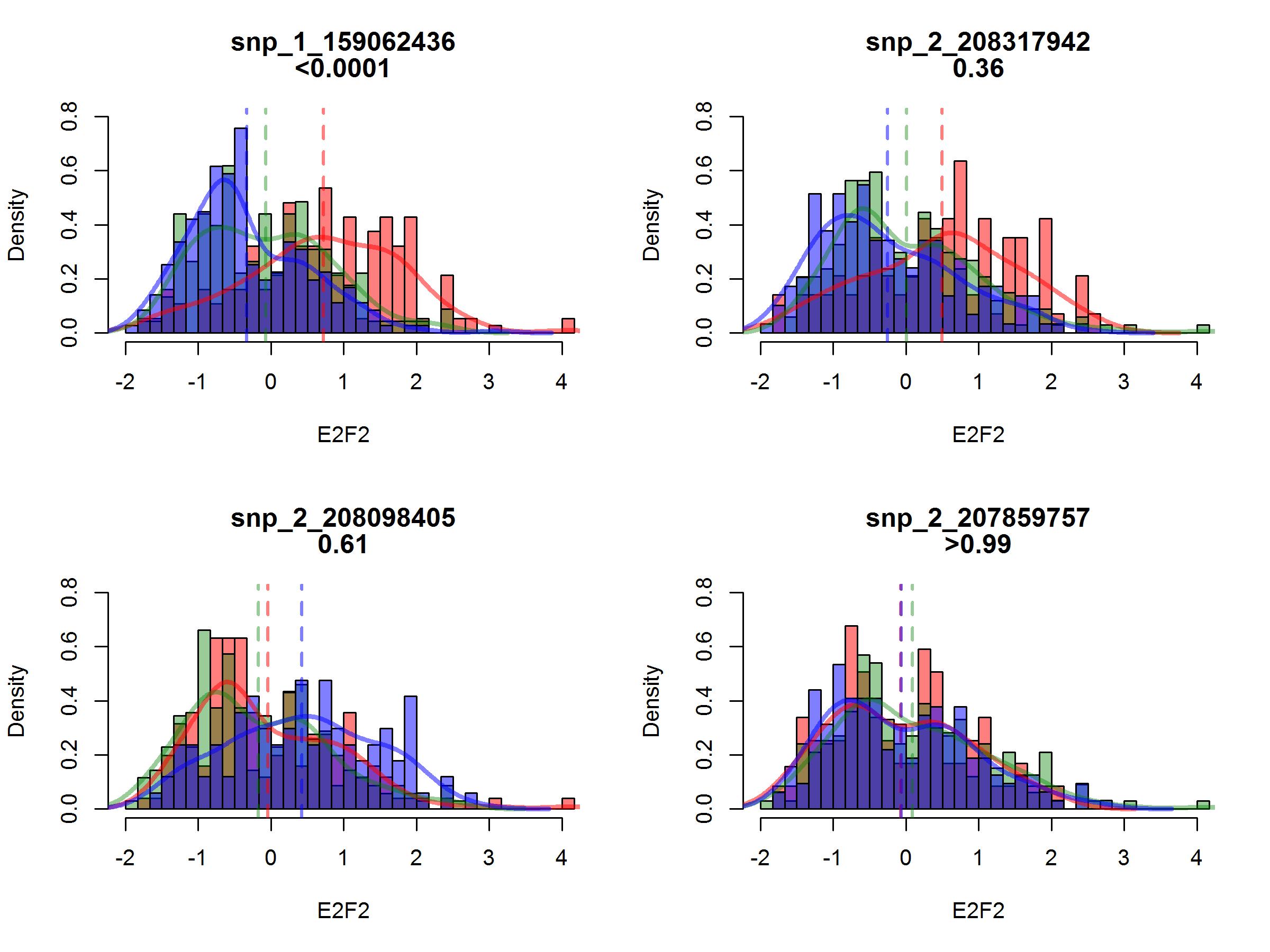
Next, we run the second stage and estimate by averaging over the baseline samples, after first removing the SNPs that contain missing data or have values being all 0, all 1 or all 2. The resulting posterior probabilities are displayed in Figure 4. Note that the majority of posterior probabilities are concentrated near 1, with roughly having a posterior probability of 0.95 or greater. On the other hand, about of posterior probabilities have values 0.05 or less, with the smallest being . Figure 5 shows the estimated densities at four selected SNPs where red represents samples with , green with and blue with . The SNPs are chosen with their at four different values of under-0.0001, 0.36, 0.61 and over-0.99. Overall, the results suggest that MOBS performs well. SNPs with close to 1 have all three estimated distributions nearly identical consistent with the raw data histograms. On the other hand, SNPs with close to 0 have three highly varying estimated densities, which are again consistent with smoothed versions of the data histograms.
Figure 4: Histogram of , measuring the association between and the SNPs.Figure 5: The estimated densities for for (red), (green) and (blue) at four selected SNPs with varying values of at under 0.0001, 0.36, 0.61 and over 0.99. Histograms are also displayed in red, green and blue for each of the three groups.
Traditional screening methods generally focus on testing the differences in mean. However, such methods miss more complex shifts in variance or density shape. MOBS is sensitive to not only mean shifts but also shifts in the shape and variance. To judge how much of the SNP selection is due to differences in means, we run the six methods MOBS, DCS, SIS, SIRS, the fused Kolmogorov filter and the JYL Bayesian nonparametric test and then select the 50 most significant predictors across all six models. For DCS, SIS, SIRS, the fused Kolmogorov filter, we convert each into and where and are 0/1 indicators for and respectively. We then run the models on both and and take the overall test statistic as the maximum of the two. Across all models, we take the sum of the absolute value of the mean for each of the three groups and and display their values in Table 1. The results show that the SNPs selected by DCS, SIS, SIRS and JYL have higher values of total absolute mean distance, which imply that they are predominantly identifying the shifts in the mean. On the other hand, MOBS and FUSEDK have significantly lower values and hence are focusing not just on the mean but on more complex differences.
MOBS
DCS
SIS
SIRS
FUSEDK
JYL
Total Absolute Mean Distance
1.12
1.88
1.91
1.86
1.14
1.64
Table 1: The sum of the absolute value of the mean of each cluster for the six models.
Finally, we assess whether the SNPs identified by MOBS have good predictive performance compared with those identified by DCS, SIS, SIRS, FUSEDK and JYL. We split the data with 370 samples for training and 92 for testing and run 5-fold cross validation. For each screening method, we select the 50 most significant SNPs. In order to examine the predictive capabilities of each method, we fit LASSO after screening. Therefore, the resulting algorithms are MOBS-L, DCS-L, SIS-L, SIRS-L, FUSEDK-L and the JYL-L and their average measure squared errors (MSE) are given in Table 2. While the nonparametric MOBS-L, JYL-L and FUSEDK-L perform better than the SIS-L, DCS-L and SIRS-L, all six methods suffer from poor predictive performance with relatively high MSE. This is not surprising as it tends to be very difficult to accurately predict gene expression based on SNPs alone. The main focus of the analysis is on identifying a promising set of SNPs for further study and not on prediction. A nice feature of MOBS is that it can pick up SNPs different from those identified by existing screening methods.
MOBS-L
DCS-L
SIS-L
SIRS-L
FUSEDK-L
JYL-L
Average MSE
0.850
0.882
0.880
0.886
0.847
0.852
Table 2: Comparison of the predictive performance of the six models using the 50 most significant predictors over .
6 Discussion
In this paper, we introduce MOBS, a Bayesian nonparametric class of screening procedures for arbitrary response and categorical predictors . By using a type of modularization, MOBS first runs an MCMC algorithm over a baseline model for the marginal response density and then uses these baseline samples to rapidly estimate each conditional density . Through simulations, MOBS performs very competitively in terms of both screening performance and computational cost. An analysis on the cis-eQTL genomics dataset reveals that MOBS is able to capture complex shifts beyond a simple difference in means, while maintaining a competitive predictive performance.
The main focus of the paper is on introducing our novel modular screening technique, and providing an illustration through univariate continuous outcome data with massive-dimensional categorical predictors; the cis-eQTL dataset analyzed in Section 5 involved roughly 38 million SNP predictors, which is orders of magnitude larger than is considered in most articles on ”high-dimensional” methods. The proposed MOBS strategy can be applied much more broadly; for example, it is straightforward to consider outcome variables that are multivariate and complex, as long as a Bayesian mixture model and MCMC algorithm has been developed for data of that type. This is the case not just for multivariate and mixed scale data but also for object data ranging from shapes and curves to graphs. It is also possible to adapt the methods to accommodate continuous or mixed categorical and continuous predictors. One approach is define pre-specified knots for each continuous predictor (e.g., spaced at quantiles of the empirical distribution of ) and use kernels to interpolate between these knots.
Acknowledgements
The authors thank Barbara Engelhardt of Princeton University for generously providing the cis-eQTL dataset used in Section 5. This research was partially funded by grant 1546130 of the US National Science Foundation (NSF) and grant 3130624 of the US Office for Naval Research (ONR).
REFERENCES
Attwooll et al. (2004)
Attwooll, C., Denchi, E. L., and Helin, K. (2004), “The E2F Family:
Specific Functions and Overlapping Interests,” The EMBO Journal, 23,
4709–4716.
Candes and Tao (2007)
Candes, E. and Tao, T. (2007), “The Dantzig Selector: Statistical
Estimation When Is Much Larger Than ,” The Annals of
Statistics, 35, 2313–2351.
Chung and Dunson (2009)
Chung, Y. and Dunson, D. B. (2009), “Nonparametric Bayes Conditional
Distribution Modeling with Variable Selection,” Journal of the American
Statistical Association, 104, 1646–1660.
Dunson and Peddada (2008)
Dunson, D. B. and Peddada, S. D. (2008), “Bayesian Nonparametric
Inference on Stochastic Ordering,” Biometrika, 95, 859–874.
Fan and Li (2001)
Fan, J. and Li, R. (2001), “Variable Selection via Nonconcave Penalized
Likelihood and Its Oracle Properties,” Journal of the American
Statistical Association, 96, 1348–1360.
Fan and Lv (2008)
Fan, J. and Lv, J. (2008), “Sure Independence Screening for Ultrahigh
Dimensional Feature Space (with Discussion),” Journal of the Royal
Statistical Society, Series B, 70, 849–911.
Fan and Song (2010)
Fan, J. and Song, R. (2010), “Sure Independence Screening in
Generalized Linear Models with NP-Dimensionality,” The Annals of
Statistics, 38, 3567–3604.
Fan et al. (2011)
Fan, J., Feng, Y., and Song, R. (2011), “Nonparametric Independence
Screening in Sparse Ultra-High Dimensional Additive Models,” Journal of
the American Statistical Association, 106, 544–557.
Filippi et al. (2016)
Filippi, S., Holmes, C., and Nieto-Barajas, L. (2016), “Scalable
Bayesian Nonparametric Measures for Exploring Pairwise Dependence via
Dirichlet Process Mixtures,” Electronic Journal of Statistics, 10,
3338–3354.
Holmes et al. (2015)
Holmes, C. C., Caron, F., Griffin, J. E., and Stephens, D. A. (2015),
“Two-Sample Bayesian Nonparametric Hypothesis Testing,”
Bayesian Analysis, 10, 297–320.
Ishwaran and Zarepour (2002)
Ishwaran, H. and Zarepour, M. (2002), “Exact and Approximate Sum
Representations for Dirichlet Process,” The Canadian Journal of
Statistics, 30, 269–283.
Jiang et al. (2017)
Jiang, B., Ye, C., and Liu, J. S. (2017), “Bayesian Nonparametric Tests
via Sliced Inverse Modeling,” Bayesian Analysis, 12, 89–112.
Kessler et al. (2014)
Kessler, D. C., Taylor, J. A., and Dunson, D. B. (2014), “Learning
Phenotype Densities Conditional on Many Interacting Predictors,”
Bioinformatics, 30, 1562–1568.
Kleijn and van der Vaart (2006)
Kleijn, B. J. K. and van der Vaart, A. W. (2006), “Misspecification in
Infinite-Dimensional Bayesian Statistics,” The Annals of Statistics,
34, 837–877.
Lappalainen et al. (2013)
Lappalainen, T., Sammeth, M., Friedländer, M. R., ‘t Hoen, P. A.,
Monlong, J., Rivas, M. A., Gonzàlez-Porta, M., Kurbatova, N., Griebel,
T., Ferreira, P. G., Barann, M., Wieland, T., Greger, L., van Iterson, M.,
Almlöf, J., Ribeca, P., Pulyakhina, I., Esser, D., Giger, T., Tikhonov,
A., Sultan, M., Bertier, G., MacArthur, D. G., Lek, M., Lizano, E., Buermans,
H. P., Padioleau, I., Schwarzmayr, T., Karlberg, O., Ongen, H., Kilpinen, H.,
Beltran, S., Gut, M., Kahlem, K., Amstislavskiy, V., Stegle, O., Pirinen, M.,
Montgomery, S. B., Donnelly, P., McCarthy, M. I., Flicek, P., Strom, T. M.,
Lehrach, H., Schreiber, S., Sudbrak, R., Carracedo, Á., Antonarakis,
S. E., Häsler, R., Syvänen, A. C., van Ommen, G. J., Brazma, A.,
Meitinger, T., Rosenstiel, P., Guigó, R., Gut, I. G., Estivill, X., and
Dermitzakis, E. T. (2013), “Transcriptome and Genome Sequencing
Uncovers Functional Variation in Humans,” Nature, 501, 506–511.
Li et al. (2012)
Li, R., Zhong, W., and Zhu, L. (2012), “Feature Screening via Distance
Correlation Learning,” Journal of the American Statistical
Association, 107, 1129–1139.
Liu et al. (2009)
Liu, F., Bayarri, M. J., and Berger, J. (2009), “Modularization in
Bayesian Analysis, with Emphasis on Analysis of Computer Models,”
Bayesian Analysis, 4, 119–150.
Lock and Dunson (2015)
Lock, E. and Dunson, D. B. (2015), “Shared Kernel Bayesian Screening,”
Biometrika, 102, 829–842.
Ma and Wong (2011)
Ma, L. and Wong, W. H. (2011), “Coupling Optional Pólya Trees and
the Two Sample Problem,” Journal of the American Statistical
Association, 106, 1553–1565.
Mai and Zou (2013)
Mai, Q. and Zou, H. (2013), “The Kolmogorov Filter for Variable
Screening in High-Dimensional Binary Classification,” Biometrika, 100,
229–234.
Mai and Zou (2015)
Mai, Q. and Zou, H. (2015), “The Fused Kolmogorov Filter: A
Nonparametric Model-Free Screening Method,” The Annals of Statistics,
43, 1471–1497.
Papastamoulis (2016)
Papastamoulis, P. (2016), “Label.Switching: An R Package for Dealing
with the Label Switching Problem in MCMC Outputs,” Journal of
Statistical Software, 69, 1–24.
Rousseau and Mengersen (2011)
Rousseau, J. and Mengersen, K. (2011), “Asymptotic Behaviour of the
Posterior Distribution in Overfitted Mixture Models,” Journal of the
Royal Statistical Society, Series B, 73, 689–710.
Scott and Berger (2010)
Scott, J. G. and Berger, J. O. (2010), “Bayes and Empirical-Bayes
Multiplicity Adjustment in the Variable-Selection Problem,” The Annals
of Statistics, 38, 2587–2619.
Stephens (2000)
Stephens, M. (2000), “Dealing with Label Switching in Mixture Models,”
Journal of the Royal Statistical Society, Series B, 62, 795–809.
Tibshirani (1996)
Tibshirani, R. (1996), “Regression Shrinkage and Selection via the
Lasso,” Journal of the Royal Statistical Society, Series B, 58,
267–288.
Yang and Dunson (2016)
Yang, Y. and Dunson, D. B. (2016), “Bayesian Conditional Tensor
Factorizations for High-Dimensional Classification,” Journal of the
American Statistical Association, 111, 656–669.
Zhu et al. (2011)
Zhu, L., Li, L., Li, R., and Zhu, L. (2011), “Model-Free Feature
Screening for Ultrahigh-Dimensional Data,” Journal of the American
Statistical Association, 106, 1464–1475.
Appendix
Algorithm for univariate Gaussian base mixture model
In this section, we provide algorithmic details to sample from the base univariate Gaussian mixture model described in Algorithm 1. Let be the number of individuals in component and be the mean of within component . We use a Gibbs sampler to update parameters using the full conditionals:
1.
Sample the cluster allocations from multinomial conditional distributions with
2.
Sample the component-specific means and variances from
where
3.
Sample the vector of weights on the different mixture components
Proof of Theorem 3.1
Lemma 6.1
As , with for some fixed , we have
where
and
where
Proof.
By Stirling’s formula, for and , we have
Thus,
When , we know
Therefore,
where
As for , we see that
Thus
Also
Thus
where
To prove Theorem 3.1, we first set and fix .
We see that for each and , for given , the integer is the number of with in component . As the event that belongs to component has probability , by Central Limit Theorem, we know
The sum can be seen as Kullback-Leibler divergence between distributions and . Under the condition for some , the Kullback-Leibler divergence . Therefore diverges to with rate .
with equality holding if and only if
Therefore, and if and only if for all . This implies under the condition , with rate of .
Under , then either or . In either case, at least one of or goes to infinity with rate or and hence with rate of .
Proof of Lemma 3.2
Lemma 6.2
. Let be independent with density . Assume exists and for all . Then, for any fixed ,
Proof.
The proof follows from Theorem 2 from Lock and Dunson (2015). Note that the positive neighborhood condition can be satisfied since has a Dirichlet prior, which induces positive support over .
The uniqueness assumption implies and . Because is continuous with respect to , there exists such that implies . Hence by the previous lemma:
(18)
.
Proof of Theorem 3.3
Since is a continuous function of and , and by the previous theorem, we know that when .
Under , , so it follows that , and , . By Theorem 3.1, , thus and hence .
On the other hand, if under , then by Theorem 3.1, , and thus and .
Proof of Theorem 3.4
By (C1), all jointly important predictors are marginally important which implies that the alternative hypothesis is true for all . Hence by (C2) and Theorem 3.3, . Thus asymptotically as , .