Randomized Benchmarking, Correlated Noise, and Ising Models
Abstract
We compute the expected randomized benchmarking sequence fidelity for a system subject to Gaussian time-correlated noise. For single qubit benchmarking we show that the expected sequence fidelity is given by the partition function of a long-range coupled spin-one Ising model, with each site in the Ising model corresponding to a free evolution interval. For -state systems, the expected sequence fidelity is given by an Ising-like model partition function whose site variables are given by the weights of the adjoint representation of SU(). A high effective temperature expansion for the partition function in the single qubit case shows decay of sequence fidelity varying from exponential for uncorrelated noise to a power law for quasistatic noise. Fitting an exponential to the sequence fidelity decay under correlated noise gives unreliable estimates of the average gate error rate.
Randomized benchmarking (RB) [1, 2, 3, 4, 5] has become a standard method for characterizing gate error rates in quantum computing. The RB protocol is simple: prepare an initial state, apply a sequence of quantum gates, measure the fidelity of the final state, repeat with sequences of increasing length, and fit the fidelity versus sequence length to an exponential to obtain the average gate error rate. The simplicity and efficiency of the protocol has led to its widespread use in many qubit technologies, including superconductors [6, 3, 7], ions [1, 8, 9], solid state quantum dots [10, 11], and atomic nuclei [12]. Though the protocol was originally developed to characterize uncorrelated Markovian noise, the qubit systems where RB has been used are generally subject to non-Markovian correlated noise [13, 14, 15, 16, 17, 18, 10, 19, 11]. In this paper we analyze the effects of correlated noise on RB. We show a surprising formal equivalence between single qubit RB and a long-range coupled spin-one Ising model. The connection to the Ising model leads to a determinant formula that gives RB sequence fidelity decays ranging from exponential to power law, depending on noise correlations.
The effects of correlated noise on RB have previously been examined, both analytically and numerically. Magesan et al. [4] as well as Wallman and Flammia [20] demonstrated the robustness of the RB estimated error rate to weakly time dependent gate noise. For correlated noise, Epstein et al. [5] showed through numerical simulations that RB gives an error rate within a factor of two of the true average gate error rate. For general Hamiltonian-driven correlated noise, Ball et al. [21] derived sequence fidelity probability density functions valid to linear order in the product of sequence length and average gate error rate . The determinant formula for the average sequence fidelity that we derive is valid for general , allowing us to quantify the degree to which sequence fidelity is nonexponential.
Our analysis shows that the expected RB sequence fidelity is given by a spin-one Ising model partition function. The Ising model has effective coupling strengths given by the covariance matrix of error phases accumulated in benchmarking intervals and an effective temperature given by the inverse of the gate error rate. We use the techniques of statistical field theory [22] to obtain a high temperature series expansion for the RB sequence fidelity, and also to make explicit the relationship between RB and random dynamical decoupling [23, 24]. The lowest order term in the high temperature expansion takes the form of a finite rank Toeplitz determinant [25], giving dependence in the sequence fidelity varying from exponential for uncorrelated noise to power law for quasistatic noise. Because fitting the power law decay to an exponential produces unreliable results, we propose an alternative fitting procedure based on the observation that the initial fidelity decay is independent of noise correlations [21]. Finally, we show that the formal equivalence between RB and long-range coupled Ising models extends to benchmarking of -state systems, with Ising model site variables that are the weights of the adjoint representation of SU().
The expected value of the RB sequence fidelity is given by the noise-averaged -fold composition of the twirled (group-averaged) free evolution operator :
| (1) |
for an initial density matrix that is a pure state. The twirled free evolution operator in interval is defined as
| (2) |
where U() is the -dimensional unitary group, is the Haar measure for U(), and is the noisy unitary free evolution in interval . The twirled free evolution operator is implemented experimentally using a unitary 2-design for U(), converting the integral over the Haar measure in Eq. (2) to a finite sum over the design. For qubit systems, the 2-design is usually the Clifford group. Eq. (1) then contains two averages: a noise average and a group (or sequence) average. We assume that these averages are independent so that each sequence sees all noise realizations. Experimentally, there may be noise correlations between sequence executions not fully captured by the present formalism.
For a single qubit subject to Hamiltonian noise, the unitary free evolution operator is , where is the error phase accumulated in free evolution interval , is a unit vector giving the axis of rotation in 3-space, and is the vector of Pauli matrices. Taking as a basis for the space of density matrices the identity matrix and Pauli matrices , the matrix representation of the twirled free evolution operator Eq. (2) is , for ; all other components are 0 [5]. For any initial pure-state density matrix the repeated application of the twirled free evolution map results in a sequence fidelity of
| (3) |
where we have defined as the noise-averaged product.
Assuming that the length vector of accumulated error phases is Gaussian distributed,
| (4) |
where is the vector of mean accumulated error phases, is the positive semi-definite covariance matrix of the noise, and is the determinant of . In the case that has zero eigenvalues, we take the distribution as giving Dirac delta functions in the directions of the eigenvectors whose associated eigenvalues are zero. We assume that the mean accumulated error phase in each interval is the same, so that , where is the length vector of all ones. Before evaluating for general covariance matrices, we examine the uncorrelated (Markovian) and quasistatic noise limits.
For noise that is uncorrelated between intervals and identical on each interval, the covariance matrix is , where parameterizes the strength of the noise (, with the average gate error rate) and is the identity matrix. Because the covariance matrix is diagonal, the -dimensional integral in Eq. (4) becomes the product of identical integrals:
| (5) |
leading to the standard exponential decay in sequence fidelity for DC and/or uncorrelated noise. For quasistatic noise, the covariance matrix is singular: it has one eigenvalue of and zero eigenvalues. Integrating over the delta functions associated with the zero eigenvalues leaves the single integral:
| (6) | |||||
| (7) |
where is a trinomial coefficient [26]. These exact expressions for uncorrelated and quasistatic noise are useful in assessing the accuracy of approximate expressions for the sequence fidelity presented below. For both uncorrelated and quasistatic noise, the case of a single free evolution interval allows us to identify as parameterizing the envelope decay of a driven oscillation . Defining to be the length in time of the free evolution interval, is related to through , with the exponent and characteristic noise time depending on the noise process, while for a DC field characterized by strength .
Returning to the general expression Eq. (4), we rewrite the product of terms as a sum of cosines:
| (8) |
Here is a length vector each of whose components is , , or ; the sum is over all configurations of . The validity of this equality can be shown by induction using the cosine addition formula. Eq. (4) then takes the form
| (9) | |||||
| (10) |
The equality of Eqs. (9) and (10) is the Hubbard-Stratonovich transformation [27, 28], used to convert an Ising model to an associated field theory. We use the inverse transformation here, converting the “field theory” of the sequence fidelity to an Ising model. The right hand side of Eq. (10) is a partition function for an -site spin-one Ising model with long-range coupling, normalized to an infinite temperature value of . Interactions between site variables have coupling strength determined by the covariance matrix , and the site couples to an imaginary magnetic field . If both and scale with , we can identify as the inverse temperature. Because it characterizes the noise strength, must be small, corresponding to the high temperature limit; otherwise a RB experiment would not be useful. Though Eq. (10) has the form of a partition function sum, it is not used in the same way that a normal partition function is used. The expected RB sequence fidelity is directly proportional to : is not used as a probability density function whose normalization is immaterial, but instead the actual value of is its key property.
Equation (10) reveals a pleasing connection between single qubit RB and a spin-one Ising model partition function. However, using Eq. (10) to determine the sequence fidelity for given and requires evaluating a sum with a number of terms exponential in the sequence length . Using as an expansion parameter, we perform a high temperature/weak coupling expansion of Eq. (4) to derive an approximate expression for the single qubit sequence fidelity, presented in the supplementary material. When the mean noise , the approximate form for the partition function is
| (11) |
where . The leading order dependence of the sequence fidelity depends only on the determinant of a symmetric positive definite matrix; for wide-sense stationary noise this matrix is also Toeplitz. Since the determinant expression is common to all terms in the series expansion, the correction terms within the parentheses specify relative errors compared to the leading order term. The first correction term nominally has scaling, with the actual scaling dependent on the covariance matrix .
For uncorrelated and quasistatic noise the Toeplitz determinants are readily computed analytically. For the case of uncorrelated noise ,
| (12) |
and the sequence fidelity decays exponentially with increasing , with error rate the same to as that given by Eq. (5). The previously stated dependence of the correction term is apparent. Though the relative error may become large for large , the absolute error will be exponentially small because of the prefactor. For the case of quasistatic noise, , and
| (13) |
The quasistatic noise sequence fidelity decays as the inverse square root of , significantly slower than in the case of uncorrelated noise. The correction term now scales as for large , so that both the relative and absolute errors of the leading order quasistatic series expansion compared to the exact expression Eq. (7) decrease with large . One may compute additional terms of the series expansion in Eq. (11) if high accuracy in sequence fidelity is required.
Uncorrelated and quasistatic noise display significantly different decay dependence on . Figure 1 shows the decay of sequence fidelity for uncorrelated and quasistatic noise computed from the exact expressions Eqs. (5) and (7), respectively, for the same noise parameter and .

Fitting the uncorrelated noise decay to the standard RB decay expression recovers the original noise parameter ; fitting the quasistatic noise decay to the leading order decay in Eq. (13) also recovers . Fitting quasistatic noise decay to gives inconsistent estimates of the noise parameter . Magenta curves in Fig. 1 show four fitting scenarios, with and held fixed or allowed to vary, and with equal weighting of sequence fidelity data or weighting by inverse sequence length in the least squares objective. All curves shown here underestimate the average gate error rate by factors of two to six; overestimation is also possible if only short RB sequence lengths are used for fitting. A more detailed analysis of fitting power law decay to an exponential is given in the supplementary information. This example demonstrates the danger in assuming that all benchmarking experiments can be fit to exponential decay.
If the form but not the overall scale of the covariance matrix is known, fitting benchmarking data to Eq. (11) estimates . With no prior knowledge of , an alternative procedure for determining or emerges from the observation that the sequence fidelity for small is independent of the noise correlations, a result previously noted in [21]. To lowest order in , Eq. (11) gives , independent of all the off-diagonal elements of the covariance matrix. The initial decay in sequence fidelity can be fit to , where is determined by the asymptotic value of for large . Fitting the quasistatic expression Eq. (7) shown in Fig. 1 with yields , a 7% relative error in the average gate error rate. Errors in fitting of and arise from the linear approximation and the error in the asymptotic value for , respectively.
If we assume that the noise is limited to a single axis, the covariance matrix can be expressed simply in terms of the noise power spectral density (PSD). For dephasing noise with Hamiltonian , the error phase accumulated in a free evolution interval is . Using the Wiener-Khinchin theorem, the covariance matrix components for , are
| (14) | |||||
where is the PSD of . Define to be the quantity in the square brackets in Eq. (14). With the effective Ising model Hamiltonian in Eq. (10) as , we recognize as giving filter functions used in dynamical decoupling analyses [21, 29, 30, 31, 32]. For a dynamical decoupling pulse sequence of length , a single configuration of site variables taking only values of or specifies the decoupling sequence and associated filter function . In the RB context, we can interpret the partition function sum Eq. (10) and corresponding sequence fidelity Eq. (3) as the average fidelity over “decoupling” (really randomization) sequences. An additional value of for each site variable is permitted by the twirled free evolution map, in contrast to dynamical decoupling where only “forward” (1) and “echoed” () intervals are allowed. This is because the twirled free evolution map takes values from the weights of the adjoint representation of SU(2) while single axis dynamical decoupling takes values from the non-trivial irreducible representation of .
| orange (uncorrelated) | – | 1 | |||
|---|---|---|---|---|---|
| brown | 1 | ||||
| purple | 2 | ||||
| red | 2 | ||||
| green | 2 | ||||
| blue (quasistatic) | – | – | – | 2 |

For a PSD of the form [33]
| (15) |
a variety of different sequence fidelity decay behaviors is possible. This continuous, piecewise PSD is constant at low frequency, at medium frequencies, and at high frequencies. For a PSD of this functional form the covariance matrix integrals Eq. (14) have (large) closed form expressions as functions of , , , and , with which approximate sequence fidelities are computed using Eq. (11). Figure 2 shows the sequence fidelity decay for four choices for the , , and parameters given in Table 1; all sequence fidelities are computed with . Uncorrelated (orange) and quasistatic (blue) sequence fidelity data are shown for comparison in Fig. 2, with all six curves having and . From , one can determine and from a -series expansion of . and for the different PSDs are also given in Table 1. Since all six curves have the same value, small behavior is almost identical. For large the decays behave differently, with the brown and purple curves exhibiting nearly uncorrelated noise behavior, and the green curve exhibiting more quasistatic noise behavior. Free evolution decay for the brown and purple PSDs are different—exponential and Gaussian, respectively, but their benchmarking decays are nearly identical. The green curve has PSD behavior at the pulsing frequency, and the red curve has PSD at the pulsing frequency; both give rise to decays between uncorrelated and quasistatic.
Finally, we note that the relationship between RB sequence fidelity and Ising model partition functions can be generalized to -state systems. The progression from Eq. (4) to Eq. (10) for is structurally the same for general : the non-trivial term in the twirled free evolution matrix is the sum of cosines over weights of the adjoint representation of SU(); products of cosine terms are converted into sums using the cosine addition formula; the Hubbard-Stratonovich transformation converts the integral over all error phases at different intervals into a partition function sum over all possible configurations of SU() adjoint representation weights at sites. The details of the analysis are given in the supplementary material.
In summary, we have shown that RB on one or more qubits has a deep connection to the Ising model and admits long-range (power law) and short range (exponential) decay behavior for noises with different spectra. On the surface, this implies that fitting RB experiments to an exponential decay model can be dangerous and can lead to undependable estimates of the error rate. This can be mitigated by fitting only the short sequence (linear decay) and asymptotic regime data, which always gives a consistent estimate of the average single gate error rate.
There is however a deeper issue. For generic noise, the average gate error rate does not uniquely determine the long time behavior. Even if we can correctly estimate the average gate error with RB we may learn nothing about a system’s fault-tolerant behavior [34]. Nonexponential RB decay implies that there exist error correction/control procedures that are more favorable than simply comparing the average gate error rate to fault tolerance thresholds, thresholds that are generally calculated using Markovian error models. A trivial example is that for perfect quasistatic noise one could completely eliminate errors with decoupling sequences, but whether there generically exist error mitigation techniques for correlated noise is an interesting open problem.
References
- [1] E. Knill, D. Leibfried, R. Reichle, J. Britton, R. B. Blakestad, J. D. Jost, C. Langer, R. Ozeri, S. Seidelin, and D. J. Wineland, Phys. Rev. A 77, 012307 (2008).
- [2] E. Magesan, J. M. Gambetta, and J. Emerson, Phys. Rev. Lett. 106, 180504 (2011).
- [3] E. Magesan, J. M. Gambetta, B. R. Johnson, C. A. Ryan, J. M. Chow, S. T. Merkel, M. P. da Silva, G. A. Keefe, M. B. Rothwell, T. A. Ohki, M. B. Ketchen, and M. Steffen, Phys. Rev. Lett. 109, 080505 (2012a).
- [4] E. Magesan, J. M. Gambetta, and J. Emerson, Phys. Rev. A 85, 042311 (2012b).
- [5] J. M. Epstein, A. W. Cross, E. Magesan, and J. M. Gambetta, Phys. Rev. A 89, 062321 (2014).
- [6] J. M. Chow, J. M. Gambetta, L. Tornberg, J. Koch, L. S. Bishop, A. A. Houck, B. R. Johnson, L. Frunzio, S. M. Girvin, and R. J. Schoelkopf, Phys. Rev. Lett. 102, 090502 (2009).
- [7] R. Barends, J. Kelly, A. Megrant, A. Veitia, D. Sank, E. Jeffrey, T. C. White, J. Mutus, A. G. Fowler, B. Campbell, Y. Chen, Z. Chen, B. Chiaro, A. Dunsworth, C. Neill, P. O/’Malley, P. Roushan, A. Vainsencher, J. Wenner, A. N. Korotkov, A. N. Cleland, and J. M. Martinis, Nature 508, 500 (2014).
- [8] J. P. Gaebler, A. M. Meier, T. R. Tan, R. Bowler, Y. Lin, D. Hanneke, J. D. Jost, J. P. Home, E. Knill, D. Leibfried, and D. J. Wineland, Phys. Rev. Lett. 108, 260503 (2012).
- [9] T. P. Harty, D. T. C. Allcock, C. J. Ballance, L. Guidoni, H. A. Janacek, N. M. Linke, D. N. Stacey, and D. M. Lucas, Phys. Rev. Lett. 113, 220501 (2014).
- [10] M. Veldhorst, J. C. C. Hwang, C. H. Yang, A. W. Leenstra, B. de Ronde, J. P. Dehollain, J. T. Muhonen, F. E. Hudson, K. M. Itoh, A. Morello, and A. S. Dzurak, Nat Nano 9, 981 (2014).
- [11] M. A. Fogarty, M. Veldhorst, R. Harper, C. H. Yang, S. D. Bartlett, S. T. Flammia, and A. S. Dzurak, Phys. Rev. A 92, 022326 (2015).
- [12] J. J. Pla, K. Y. Tan, J. P. Dehollain, W. H. Lim, J. J. L. Morton, F. A. Zwanenburg, D. N. Jamieson, A. S. Dzurak, and A. Morello, Nature 496, 334 (2013).
- [13] F. C. Wellstood, C. Urbina, and J. Clarke, Applied Physics Letters 50, 772 (1987), http://dx.doi.org/10.1063/1.98041 .
- [14] F. Yoshihara, K. Harrabi, A. O. Niskanen, Y. Nakamura, and J. S. Tsai, Phys. Rev. Lett. 97, 167001 (2006).
- [15] J. Bylander, S. Gustavsson, F. Yan, F. Yoshihara, K. Harrabi, G. Fitch, D. G. Cory, Y. Nakamura, J.-S. Tsai, and W. D. Oliver, Nat Phys 7, 565 (2011).
- [16] D. H. Slichter, R. Vijay, S. J. Weber, S. Boutin, M. Boissonneault, J. M. Gambetta, A. Blais, and I. Siddiqi, Phys. Rev. Lett. 109, 153601 (2012).
- [17] S. M. Anton, J. S. Birenbaum, S. R. O’Kelley, V. Bolkhovsky, D. A. Braje, G. Fitch, M. Neeley, G. C. Hilton, H.-M. Cho, K. D. Irwin, F. C. Wellstood, W. D. Oliver, A. Shnirman, and J. Clarke, Phys. Rev. Lett. 110, 147002 (2013).
- [18] J. M. Taylor, J. R. Petta, A. C. Johnson, A. Yacoby, C. M. Marcus, and M. D. Lukin, Phys. Rev. B 76, 035315 (2007).
- [19] K. Eng, T. D. Ladd, A. Smith, M. G. Borselli, A. A. Kiselev, B. H. Fong, K. S. Holabird, T. M. Hazard, B. Huang, P. W. Deelman, I. Milosavljevic, A. E. Schmitz, R. S. Ross, M. F. Gyure, and A. T. Hunter, Science Advances 1, e1500214 (2015).
- [20] J. J. Wallman and S. T. Flammia, New Journal of Physics 16, 103032 (2014).
- [21] H. Ball, T. M. Stace, S. T. Flammia, and M. J. Biercuk, Phys. Rev. A 93, 022303 (2016).
- [22] D. J. Amit, Field Theory, the Renormalization Group, and Critical Phenomena; 3rd ed. (World Scientific, Singapore, 2005).
- [23] L. Viola, E. Knill, and S. Lloyd, Phys. Rev. Lett. 82, 2417 (1999).
- [24] L. Viola and E. Knill, Phys. Rev. Lett. 94, 060502 (2005).
- [25] M. E. Fisher and R. E. Hartwig, “Toeplitz determinants: Some applications, theorems, and conjectures,” (John Wiley & Sons, Inc., 2007) pp. 333–353.
- [26] L. Euler, in Opera Omnia, Series Prima, Vol. 15 (Teubner, Leipzig, Germany, 1911) pp. 50–69.
- [27] R. L. Stratonovich, Soviet Physics Doklady 2, 416 (1957).
- [28] J. Hubbard, Phys. Rev. Lett. 3, 77 (1959).
- [29] Ł. Cywiński, R. M. Lutchyn, C. P. Nave, and S. D. Sarma, Phys. Rev. B 77, 174509 (2008).
- [30] M. J. Biercuk, A. C. Doherty, and H. Uys, Journal of Physics B: Atomic, Molecular and Optical Physics 44, 154002 (2011).
- [31] T. Green, H. Uys, and M. J. Biercuk, Phys. Rev. Lett. 109, 020501 (2012).
- [32] T. J. Green, J. Sastrawan, H. Uys, and M. J. Biercuk, New Journal of Physics 15, 095004 (2013).
- [33] E. Paladino, Y. M. Galperin, G. Falci, and B. L. Altshuler, Rev. Mod. Phys. 86, 361 (2014).
- [34] R. Kueng, D. M. Long, A. C. Doherty, and S. T. Flammia, Phys. Rev. Lett. 117, 170502 (2016).
Randomized Benchmarking, Correlated Noise, and Ising Models:
Supplementary Material
I High Effective Temperature Expansion for Partition Function
Here we derive the approximate expression, Eq. (11) of the main text, for the single qubit sequence fidelity partition function discussed in the main text. Our starting point is Eq. (4) of the main text,
| (1) |
We define new integration variables , where ( is the standard deviation of the random noise in each free evolution interval). Here we are using to parameterize the strength of the random noise only; can take finite values, independent of the size of the random noise. With respect to the spin-one Ising model, only really represents an effective inverse temperature when also scales with . By excluding scaling from , however, we can obtain approximate expressions that hold for small random noise (small ) and finite mean .
We expand the product in the square brackets in Eq. (1) in an series,
| (2) | |||||
This series expansion is obtained by taking the exponential of the Taylor series expansion of the logarithm of the left hand side product, keeping the first and second orders in in the exponential, and re-expanding in a Taylor series the exponential of all the remaining terms in the logarithm expansion. Such an expansion plays a similar role to the expansion of in field theory. The expansion allows us to express all terms in the integral of Eq. (1) as moments of a Gaussian distribution with modified covariance matrix and modified mean ,
| (3) | |||||
| (4) | |||||
| (5) |
Notice that retains the scaling of and that also is first order in . Performing the Gaussian moment integrations (Wick contractions) and setting results in the following series expansion for the partition function:
| (6) | |||||
In the limit of zero mean noise , and . The approximate form for the partition function then becomes
| (7) |
Eq. (11) in the main text.
II Fitting Quasistatic Noise Sequence Fidelity Decay to an Exponential
In this section we illustrate the inconsistencies in fitting quasistatic sequence fidelity decay to an exponential. We assume that the quasistatic sequence fidelity decay is described by the lowest order term in the approximate partition function, Eq. (13) of the main text, with the nominal average gate error rate . With “data” generated from Eq. (13) of the main text, we perform a weighted least-squares fit to an exponential functional form minimizing the objective
| (8) |
where , , and are the possible fitting parameters, and is the maximum RB sequence length used in the fit. measures how far the fit deviates from the nominal average gate error rate .
We consider four fitting scenarios:
- 1.
and are fixed at and
- 2.
and are fixed at and
- 3.
and are fitting parameters and
- 4.
and are fitting parameters and .
Scenarios 1 and 3 are equally weighted with respect to sequence length, while scenarios 2 and 4 have shorter sequences more heavily weighted than longer sequences, corresponding to fitting to sequence lengths that are evenly sampled in . For the figures that follow, we take and correspondingly, . For exponential decay, corresponds to the sequence length giving the -point.
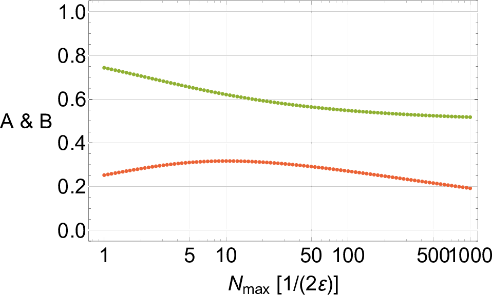
Figures 1 and 2 show the inverse of the error rate deviation parameter for the four fitting scenarios, as a function of maximum RB sequence length used in the fits. Both over- and underestimation of the average gate error rate is possible, dependent on the maximum sequence lengths used for fitting, and whether and are allowed to vary. For scenarios 3 and 4, where and are allowed to vary, and can differ substantially from their nominal values of . For scenario 3, equally weighted data, as increases, the objective is minimized by correctly fitting the nominal value of , and severely underestimating both and the average gate error rate since most of the fitting data is at large RB sequence lengths. For scenario 4, which weights shorter sequences more heavily, and are approaching their nominal values as increases, with the average gate error rate underestimated by a factor of . Note that the objective Eq. (8) is almost scale invariant for small —the summand depends on the product rather than and separately. Figures 1–4 are essentially unchanged for different values of (small) .
Figure 5 shows fits to the quasistatic sequence fidelity for scenario 4, for four different values of . For (blue curve in figure) the fit appears to be very good, but is incorrect: , , and , giving a factor of overestimate of the average gate error rate. Because and are allowed to vary, the initial nonexponential decay can be fit by changing and from their nominal values. When longer sequences are included in the fitting data, the exponential functional fitting form no longer can be made to match the full nonexponential decay.




III Benchmarking of -State Systems
Here we show that the analysis of single qubit benchmarking and its relationship to the Ising model can be extended to the benchmarking of -state systems. Following the derivation in the main text, we compute the expected benchmarking sequence fidelity in Eq. (1) of the main text, via the repeated application of the twirled free evolution operator. Because the Haar measure integration in the definition of the twirled free evolution operator (Eq. (2) of the main text) is translation invariant, without loss of generality we assume a diagonal free evolution unitary in ,
| (9) |
where is the error phase accumulated on the state in the interval. (Note that the error phase angle convention here differs from the standard SU(2) expression by a factor of 2.) This free evolution matrix can be substituted into Eq. (2) of the main text, and the integration over the Haar measure performed explicitly; however, a few group theoretical observations obviate the need for explicitly performing -dimensional integrals.
The action of the twirled free evolution map on a density matrix is the product of the defining and conjugate representations of SU(), which in turn is the direct sum of the (irreducible) trivial and adjoint representations. The twirled free evolution map in any irreducible representation (irrep) commutes with all elements in the irrep, again because of Haar measure invariance. By Schur’s lemma, the twirled free evolution map must be proportional to the identity on each irrep. The proportionality constant for each irrep is given by
| (10) |
Taking the trace of both sides gives where is the character of the free evolution operator on the irrep , and is the dimension of irrep . The character can be written in terms of the weights of irrep and the angles of [1, 2]. (The Weyl character formula is customarily used to express in terms of the highest weight of , the Cartan subalgebra, and a sum over the Weyl group, but to perform the integrations over Gaussian distributed variables, it is more convenient to express the character explicitly as a sum over all the weights.)
For the trivial and adjoint irreps, in a basis of Hermitian matrices orthogonal with respect to the trace inner product, the matrix for the twirled free evolution map is then
| (11) |
where we assume that (i.e., the upper left block of corresponds to the trivial irrep, and the lower right block of corresponds to the adjoint irrep), and is the multiset of weights of the SU() adjoint representation, in the standard basis. Adjoint representation weights in the standard basis are -component vectors with either all zero entries (of which there are repeated weights), or two non-zero entries of and (of which there are unique weights).
Repeated application of the twirled free evolution map to a pure state, again assuming a Gaussian distribution for the noise, results in cosine-weighted Gaussian integrals for the expected sequence fidelity. As in the case, we convert products of cosines into sums using the cosine addition formula, and we again use the (inverse) Hubbard-Stratonovich transformation to convert the continuous error phase variables to discrete weight variables. The final sequence fidelity expression is
| (12) |
The tensor gives the covariance between the error phase at state and free evolution interval , and the error phase at state and free evolution interval , and is the mean error accumulated in state in interval . We again have an site Ising model partition function, where each site variable is a -dimensional vector, whose possible states are the weights of the adjoint representation of SU(). Specializing to recovers the single qubit partition function of Eq. (10) of the main text.
References
- [1] J. Elliott and P. Dawber, Symmetry in Physics, Volume 2, Further Applications (Oxford University Press, New York, 1979).
- [2] R. Cahn, Semi-Simple Lie Algebras and Their Representations, Frontiers in Physics (Benjamin-Cummings Publishing Company, 1984).