跳到论文正文
W Papers独立论文阅读器 arXiv:1703.09532 论文正文 计算阅读时间 · 0%
引用这篇论文根据当前论文元数据生成,正式投稿前建议核对。


License: arXiv.org perpetual non-exclusive license
arXiv:1703.09532v1 [hep-ph] 28 Mar 2017

red

DESY 17-045
Three-loop evolution equation for flavor-nonsinglet operators in off-forward kinematics

V. M. Braun Affiliation:  Institut für Theoretische Physik, Universität Regensburg
D-93040 Regensburg, Germany
Email: alexander.manashov@desy.de
   A. N. Manashov Affiliation:  Institut für Theoretische Physik, Universität Regensburg
D-93040 Regensburg, Germany
Affiliation:  Institut für Theoretische Physik, Universität Hamburg
D-22761 Hamburg, Germany
Email: sven-olaf.moch@desy.de
   S. Moch Affiliation:  Institut für Theoretische Physik, Universität Hamburg
D-22761 Hamburg, Germany
Email: matthias.strohmaier@ur.de
   and M. Strohmaier Affiliation:  Institut für Theoretische Physik, Universität Regensburg
D-93040 Regensburg, Germany
Abstract

Using the approach based on conformal symmetry we calculate the three-loop (NNLO) contribution to the evolution equation for flavor-nonsinglet leading twist operators in the MS¯\overline{\text{MS}} scheme. The explicit expression for the three-loop kernel is derived for the corresponding light-ray operator in coordinate space. The expansion in local operators is performed and explicit results are given for the matrix of the anomalous dimensions for the operators up to seven covariant derivatives. The results are directly applicable to the renormalization of the pion light-cone distribution amplitude and flavor-nonsinglet generalized parton distributions.

Keywords
evolution equation, conformal symmetry, generalized parton distribution, pion distribution amplitude

1 Introduction

The remarkable progress in experimental techniques in the past two decades has provided a fresh impetus to the study of hard exclusive and semi-inclusive reactions with identified particles in the final state. Such processes are interesting as they allow one to access the hadron structure on a much more detailed level as compared to totally inclusive reactions. A (probably still distant) major goal is to understand the full three-dimensional proton structure by “holographic imaging” of quark and gluon distributions in transverse distance and momentum spaces. The related experiments have become a prominent part of the research program at all major existing and planned accelerator facilities, e.g. the Electron Ion Collider (EIC) [1].

The relevant nonperturbative input in such processes in many cases involves operator matrix elements between states with different momenta, dubbed generalized parton distributions (GPDs), or vacuum-to-hadron matrix elements related to light-front hadron wave functions at small trans- verse separations, the distribution amplitudes (DAs). The scale-dependence of such distributions is governed by the renormalization group (RG) equations for the corresponding operators, where, in contrast to standard parton densities, mixing with the operators involving total derivatives has to be taken into account. Going over to local operators one has to deal with a triangular mixing matrix where the diagonal entries are the anomalous dimensions, the same as in deep-inelastic scattering, but the off-diagonal elements require a separate calculation.

The projected very high accuracy of future experimental data, e.g. on the Deeply Virtual Compton Scattering (DVCS) at the JLAB 12 GeV upgrade [2] and the EIC, and the γ∗→π​γ\gamma^{*}\to\pi\gamma transition form factor at Belle II at KEK [3], has to be matched by the increasing theoretical precision; in the ideal case one would like to reach the same level of accuracy as in inclusive reactions. The NNLO (three-loop) analysis of parton distributions and fragmentation functions is becoming the standard in this field [4], so that the NNLO evolution equations for off-forward distributions are appearing on the agenda.

In this work we derive the explicit expression for the three-loop contribution to the flavor-nonsinglet evolution kernel in the so-called light-ray operator representation. This kernel can be converted to the evolution equation for the GPDs by a Fourier transformation, whereas its expansion at small distances provides one with the matrix of the anomalous dimensions for local leading twist operators. In the latter form, our results are directly relevant for the lattice calculations of pion DAs in which case the uncertainty due to the conversion of lattice results to the MS¯\overline{\text{MS}} scheme currently proves to be one of the dominant sources of the error [5]. The three-loop (NNLO) anomalous dimensions of the leading-twist operators are known for about a decade [6], however, a direct calculation of the missing off-diagonal terms in the mixing matrix to the same precision is quite challenging.

Conformal symmetry of the QCD Lagrangian allows one to restore the nondiagonal entries in the mixing matrix and, hence, full evolution kernels at a given order of perturbation theory from the calculation of the special conformal anomaly at one order less [7]. This result was used to calculate the complete two-loop mixing matrix for twist-two operators in QCD [8, 9, 10], and to derive the two-loop evolution kernels for the GPDs [11, 12, 13].

In Ref. [14] we have proposed to use a somewhat different technique to implement the same idea. Instead of studying conformal symmetry breaking in the physical theory [8, 9, 10] we suggest to make use of the exact conformal symmetry of large-nfn_{f} QCD in d=4−2​ϵd=4-2\epsilon dimensions at critical coupling. Due to specifics of the minimal subtraction scheme (MS¯\overline{\text{MS}}) the renormalization group equations in the physical four-dimensional theory inherit a conformal symmetry so that the evolution kernel commutes with the generators of conformal transformations. This symmetry is exact, however, the generators are modified by quantum corrections and differ from their canonical form. The consistency relations that follow from the conformal algebra can be used in order to restore the ℓ\ell-loop off-forward kernel from the ℓ\ell-loop anomalous dimensions and the (ℓ−1)(\ell-1)-loop result for the deformation of the generators, which is equivalent to the statement in Ref. [7].

Exact conformal symmetry of modified QCD allows one to use algebraic group-theory methods to resolve the constraints on the operator mixing and also suggests the optimal representation for the results in terms of light-ray operators. In this way one avoids the need to restore the evolution kernels from the results for local operators, which is not straightforward. This modified approach was tested in [14] on several examples to two- and three-loop accuracy for scalar theories, and in [15] for flavor-nonsinglet operators in QCD to two-loop accuracy. As a major step towards the NNLO calculation, in [16] we have calculated the two-loop quantum correction to the generator of special conformal transformations. In this work we use this result to obtain the three-loop (NNLO) evolution equation for flavor-nonsinglet leading twist operators in the light-ray operator representation in the MS¯\overline{\text{MS}} scheme. The relation to the representation in terms of local operators [7, 8, 9] is worked out in detail and explicit results are given for the matrix of the anomalous dimensions for the operators with up to seven covariant derivatives. Our results are directly applicable e.g. to the studies of the pion light-cone DA and flavor-nonsinglet GPDs.

The presentation is organized as follows. Sect. 2 is introductory, it contains a very short general description of the light-ray operator formalism and the conformal algebra. In this section we also explain our notation and conventions. In Sect. 3 we show that the contributions to the evolution kernel due to the conformal anomaly can be isolated by a similarity transformation. As the result, the evolution kernel can be written as a sum of several contributions with a simpler structure. This construction is similar in spirit to the “conformal scheme” of Refs. [8, 9, 10]. We find that the remaining (canonically) S​L​(2)SL(2)-invariant part of the three-loop kernel satisfies the reciprocity relation [17, 18, 19, 20], discussed in Sect. 4. The explicit construction of the invariant kernel is presented in Sect. 5. We provide analytic expressions for the terms that correspond to the leading asymptotic behavior at small and large Bjorken xx, and a simple parametrization for the remainder that has sufficient accuracy for all potential applications. In Sect. 6 we explain how our results for the renormalization of light-ray operators can be translated into anomalous dimension matrices for local operators. In this way also the formal relation to the results in [7, 8, 9] is established. The final Sect. 7 is reserved for a summary and outlook. The paper also contains several Appendices where we collect the analytic expressions for the kernels.

2 Evolution equations for light-ray operators

A renormalized light-ray operator,

[𝒪]​(x,z1,z2)=Z​𝒪​(x,z1,z2)=Z​q¯​(x+z1​n)​n̸​q​(x+z2​n),\displaystyle[\mathcal{O}](x;z_{1},z_{2})=Z\mathcal{O}(x;z_{1},z_{2})=Z\bar{q}(x+z_{1}n)\not{n}q(x+z_{2}n), (1)

where the Wilson line is implied between the quark fields on the light-cone, is defined as the generating function for renormalized local operators:

[𝒪]​(x,z1,z2)\displaystyle[\mathcal{O}](x;z_{1},z_{2}) ≡\displaystyle\equiv ∑m,kz1m​z2km!​k![q¯(x)(D←⋅n)mn̸(n⋅D→)kq(x)],\displaystyle\sum_{m,k}\frac{z_{1}^{m}z_{2}^{k}}{m!k!}\left[\bar{q}(x)(\stackrel{{\scriptstyle\leftarrow}}{{D}}\!\cdot n)^{m}\not{n}(n\cdot\!\stackrel{{\scriptstyle\rightarrow}}{{D}})^{k}q(x)\right], (2)

where Dμ=∂μ−igAμD_{\mu}=\partial_{\mu}-igA_{\mu} is the covariant derivative. Here and below we use square brackets to denote renormalized composite operators (in a minimal subtraction scheme). Due to Poincare invariance in most situations one can put x=0x=0 without loss of generality; we will therefore often drop the xx dependence and write

𝒪⁡(z1,z2)≡𝒪⁡(0,z1,z2).\mathcal{O}(z_{1},z_{2})\equiv\mathcal{O}(0;z_{1},z_{2}).

The renormalization factor ZZ is an integral operator in z1,z2z_{1},z_{2} which is given by a series in 1/ϵ1/\epsilon, d=4−2​ϵd=4-2\epsilon,

Z=1+∑k=0∞1ϵk​Zk​(a),\displaystyle Z=1+\sum_{k=0}^{\infty}\frac{1}{\epsilon^{k}}Z_{k}(a)\,, Zk​(a)=∑ℓ=k∞aℓ​Zk(ℓ).\displaystyle Z_{k}(a)=\sum_{\ell=k}^{\infty}a^{\ell}Z_{k}^{(\ell)}\,. (3)

The RG equation for the light-ray operator [𝒪][\mathcal{O}] takes the form

(M∂M+β(a)∂a+ℍ(a))[𝒪](x;z1,z2)=0,\displaystyle\Big(M{\partial_{M}}+\beta(a)\partial_{a}+\mathbb{H}(a)\Big)[\mathcal{O}](x;z_{1},z_{2})=0\,, (4)

where MM is the renormalization scale,

a\displaystyle a =αs4​π,β⁡(a)=M​d​ad​M=−2​a​(ϵ+a​β0+a2​β1+…)=−2​a​(ϵ+β¯​(a))\displaystyle=\frac{\alpha_{s}}{4\pi}\,,\qquad\beta(a)=M\frac{da}{dM}=-2a\big(\epsilon+a\beta_{0}+a^{2}\beta_{1}+\ldots\big)=-2a(\epsilon+\bar{\beta}(a))\, (5)

with

β0\displaystyle\beta_{0} =113​Nc−23​nf,\displaystyle=\frac{11}{3}N_{c}-\frac{2}{3}n_{f}\,, β1=23​[17​CA2−5​CA​nf−3​CF​nf].\displaystyle\beta_{1}=\frac{2}{3}\left[17C_{A}^{2}-5C_{A}n_{f}-3C_{F}n_{f}\right]\,. (6)

ℍ⁡(a)\mathbb{H}(a) is an integral operator acting on the light-cone coordinates of the fields, which has a perturbative expansion

ℍ⁡(a)\displaystyle\mathbb{H}(a) =a​ℍ(1)+a2​ℍ(2)+a3​ℍ(3)+…\displaystyle=a\,\mathbb{H}^{(1)}+a^{2}\,\mathbb{H}^{(2)}+a^{3}\,\mathbb{H}^{(3)}+\ldots (7)

It is related to the renormalization factor (3) as follows

ℍ⁡(a)=−M​dd​M​ℤ​ℤ−1=2​γq​(a)+2​∑ℓ=1∞ℓ​aℓ​Z1(ℓ),\displaystyle\mathbb{H}(a)=-M\frac{d}{dM}\mathbb{Z}\mathbb{Z}^{-1}=2\gamma_{q}(a)+2\sum_{\ell=1}^{\infty}\ell\,a^{\ell}Z_{1}^{(\ell)}\,, (8)

where ℤ=Z​Zq−2\mathbb{Z}=ZZ_{q}^{-2}; ZqZ_{q} is the quark wave function renormalization factor and γq=M​∂Mln⁡Zq\gamma_{q}=M\partial_{M}\ln Z_{q} the quark anomalous dimension. The QCD β\beta-function β⁡(a)\beta(a) and γq\gamma_{q} are known to 𝒪⁡(a5)\mathcal{O}(a^{5}) [21, 22, 23, 24, 25].

The evolution operator can be written as [26]

ℍ⁡(a)​[𝒪]​(z1,z2)=∫01d​α​∫01d​β​h​(α,β)​[𝒪]​(z12α,z21β),\displaystyle\mathbb{H}(a)[\mathcal{O}](z_{1},z_{2})=\int_{0}^{1}\!d\alpha\int_{0}^{1}\!d\beta\,h(\alpha,\beta)\,[\mathcal{O}](z_{12}^{\alpha},z_{21}^{\beta})\,, (9)

where

z12α=z1​α¯+z2​α\displaystyle z_{12}^{\alpha}=z_{1}\bar{\alpha}+z_{2}\alpha α¯=1−α,\displaystyle\bar{\alpha}=1-\alpha\,, (10)

and h⁡(α,β)=a​h(1)​(α,β)+a2​h(2)​(α,β)+…h(\alpha,\beta)=a\,h^{(1)}(\alpha,\beta)+a^{2}h^{(2)}(\alpha,\beta)+\ldots is a certain weight function (evolution kernel).

It is easy to see [14] that translation-invariant polynomials (z1−z2)N(z_{1}-z_{2})^{N} are eigenfunctions of the evolution kernel,

ℍ⁡(a)​z12N\displaystyle\mathbb{H}(a)z_{12}^{N} =γN​(a)​z12Nz12=z1−z2.\displaystyle=\gamma_{N}(a)\,z_{12}^{N}\qquad\qquad z_{12}=z_{1}-z_{2}\,. (11)

The eigenvalues γN​(a)\gamma_{N}(a) correspond to moments of the evolution kernel in the representation (9),

γN\displaystyle\gamma_{N} =∫01d​α​∫01d​β​(1−α−β)N​h​(α,β)=a​γN(1)+a2​γN(2)+a3​γN(3)+….\displaystyle=\int_{0}^{1}\!d\alpha\int_{0}^{1}\!d\beta\,(1-\alpha-\beta)^{N}h(\alpha,\beta)=a\gamma_{N}^{(1)}+a^{2}\gamma_{N}^{(2)}+a^{3}\gamma_{N}^{(3)}+\ldots\,. (12)

They define the anomalous dimensions of leading-twist local operators in Eq. (2) where N=m+kN=m+k is the total number of covariant derivatives acting either on the quark or the antiquark field. The corresponding mixing matrix in the Gegenbauer polynomial basis is constructed in Sect. 6.

The leading-order (LO) result for the evolution kernel in this representation reads [26]:

ℍ(1)​f​(z1,z2)\displaystyle\mathbb{H}^{(1)}f(z_{1},z_{2}) =4CF{∫01dαα¯α[2f(z1,z2)−f(z12α,z2)−f(z1,z21α)]\displaystyle=4C_{F}\biggl\{\int_{0}^{1}d\alpha\frac{\bar{\alpha}}{\alpha}\Big[2f(z_{1},z_{2})-f(z_{12}^{\alpha},z_{2})-f(z_{1},z_{21}^{\alpha})\Big]
−∫01dα∫0α¯dβf(z12α,z21β)+12f(z1,z2)}.\displaystyle\quad-\int_{0}^{1}d\alpha\int_{0}^{\bar{\alpha}}d\beta\,f(z_{12}^{\alpha},z_{21}^{\beta})+\frac{1}{2}f(z_{1},z_{2})\biggr\}\,. (13)

The expression in Eq. (13) gives rise to all classical leading-order (LO) QCD evolution equations: the DGLAP equation for parton distributions, the ERBL equation for the meson light-cone DAs, and the general evolution equation for GPDs.

The LO evolution kernel ℍ(1)\mathbb{H}^{(1)} commutes with the (canonical) generators of collinear conformal transformations

S−(0)\displaystyle S^{(0)}_{-} =−∂z1−∂z2,\displaystyle=-\partial_{z_{1}}-\partial_{z_{2}}\,,
S0(0)\displaystyle S^{(0)}_{0} =z1∂z1+z2∂z2+2,\displaystyle=z_{1}\partial_{z_{1}}+z_{2}\partial_{z_{2}}+2,
S+(0)\displaystyle S^{(0)}_{+} =z12∂z1+z22∂z2+2(z1+z2)\displaystyle=z_{1}^{2}\partial_{z_{1}}+z_{2}^{2}\partial_{z_{2}}+2(z_{1}+z_{2})\, (14)

which satisfy the usual S​L​(2)SL(2) algebra

[S0,S±]=±S±,\displaystyle{}[S_{0},S_{\pm}]=\pm S_{\pm}\,, [S+,S−]=2​S0.\displaystyle{}[S_{+},S_{-}]=2S_{0}\,. (15)

It can be shown that as a consequence of the commutation relations [ℍ(1),Sα(0)]=0[\mathbb{H}^{(1)},S^{(0)}_{\alpha}]=0 the corresponding kernel h(1)​(α,β)h^{(1)}(\alpha,\beta) is effectively a function of one variable τ\tau called the conformal ratio [27]

h(1)​(α,β)=h¯​(τ),\displaystyle h^{(1)}(\alpha,\beta)=\bar{h}(\tau)\,, τ=α​βα¯​β¯,\displaystyle\tau=\frac{\alpha\beta}{\bar{\alpha}\bar{\beta}}\,, (16)

up to trivial terms ∼δ⁡(α)​δ​(β)\sim\delta(\alpha)\delta(\beta) that correspond to the unit operator. This function can easily be reconstructed from its moments (12), alias from the anomalous dimensions.

Indeed, it is easy to verify that the result in Eq. (13) can be written in the following, remarkably simple form [27]

h(1)​(α,β)=−4​CF​[δ+​(τ)+θ⁡(1−τ)−12​δ​(α)​δ​(β)],\displaystyle h^{(1)}(\alpha,\beta)=-4C_{F}\left[\delta_{+}(\tau)+\theta(1-\tau)-\frac{1}{2}\delta(\alpha)\delta(\beta)\right], (17)

where the regularized δ\delta-function, δ+​(τ)\delta_{+}(\tau), is defined as

∫d​α​𝑑β​δ+​(τ)​f​(z12α,z21β)\displaystyle\int d\alpha d\beta\,\delta_{+}(\tau)f(z_{12}^{\alpha},z_{21}^{\beta}) ≡∫01d​α​∫01d​β​δ​(τ)​[f⁡(z12α,z21β)−f⁡(z1,z2)]\displaystyle\equiv\int_{0}^{1}d\alpha\int_{0}^{1}d\beta\,\delta(\tau)\Big[f(z_{12}^{\alpha},z_{21}^{\beta})-f(z_{1},z_{2})\Big]
=−∫01dαα¯α[2f(z1,z2)−f(z12α,z2)−f(z1,z21α)].\displaystyle=-\int_{0}^{1}d\alpha\frac{\bar{\alpha}}{\alpha}\Big[2f(z_{1},z_{2})-f(z_{12}^{\alpha},z_{2})-f(z_{1},z_{21}^{\alpha})\Big]. (18)

Beyond the LO this property is lost. However, the evolution kernels for leading twist operators in minimal subtraction schemes retain exact conformal symmetry. Indeed, the renormalization factors for composite operators in this scheme do not depend on ϵ\epsilon by construction. As a consequence, the anomalous dimension matrices in QCD in four dimensions are exactly the same as in QCD in d=4−2​ϵd=4-2\epsilon dimensions that enjoys conformal symmetry for the specially chosen “critical” value of the coupling [14, 15, 16]. The precise statement is that the QCD evolution kernel ℍ⁡(a)\mathbb{H}(a) commutes with three operators

[ℍ⁡(a),S+]=[ℍ⁡(a),S−]=[ℍ⁡(a),S0]=0\displaystyle[\mathbb{H}(a),S_{+}]~=~[\mathbb{H}(a),S_{-}]~=~[\mathbb{H}(a),S_{0}]~=~0 (19)

that satisfy the S​L​(2)SL(2) algebra (15). These operators can be constructed as the generators of collinear conformal transformations in the 4−2​ϵ4-2\epsilon-dimensional QCD at the critical point and have the following structure [14, 15, 16]:

S−\displaystyle S_{-} =S−(0),\displaystyle=S_{-}^{(0)}\,, (20a)
S0\displaystyle S_{0}\, =S0(0)+Δ​S0=S0(0)+(β¯​(a)+12​ℍ​(a)),\displaystyle=S_{0}^{(0)}+\Delta S_{0}~=~S_{0}^{(0)}+\left(\bar{\beta}(a)+\frac{1}{2}\mathbb{H}(a)\right)\,, (20b)
S+\displaystyle S_{+} =S+(0)+Δ​S+=S+(0)+(z1+z2)​(β¯​(a)+12​ℍ​(a))+(z1−z2)​Δ​(a),\displaystyle=S_{+}^{(0)}+\Delta S_{+}~=~S_{+}^{(0)}+(z_{1}+z_{2})\left(\bar{\beta}(a)+\frac{1}{2}\mathbb{H}(a)\right)+(z_{1}-z_{2})\,\Delta(a)\,, (20c)

where β¯​(a)\bar{\beta}(a) is the QCD β\beta-function (5) and Sα(0)S_{\alpha}^{(0)} are the canonical generators (14).

Note that the generator S−S_{-} corresponds to translations along the light cone and does not receive any corrections as compared to its canonical expression, S−(0)S_{-}^{(0)}. The generator S0S_{0} corresponds to dilatations; its modification in interacting theory Δ​S0=S0−S0(0)\Delta S_{0}=S_{0}-S_{0}^{(0)} can be related to the evolution kernel ℍ⁡(a)\mathbb{H}(a) from general considerations [14]. Finally S+S_{+} is the generator of special conformal transformations and Eq. (20c) is the most general expression consistent with the commutation relations (15). To see that, note that Δ​S+=S+−S+(0)\Delta S_{+}=S_{+}-S_{+}^{(0)} must have the same canonical dimension [mass]−1[\text{mass}]^{-1} as S+(0)S_{+}^{(0)}, meaning that [S0(0),Δ​S+]=Δ​S+[S_{0}^{(0)},\Delta S_{+}]=\Delta S_{+}. Thus we can write Δ​S+=(z1+z2)​Δ1+(z1−z2)​Δ2\Delta S_{+}=(z_{1}+z_{2})\Delta_{1}+(z_{1}-z_{2})\Delta_{2} where [S0(0),Δ1,2]=0[S_{0}^{(0)},\Delta_{1,2}]=0. Plugging this expression in the commutation relation [S+,S−]=2​S0[S_{+},S_{-}]=2S_{0} one obtains Δ1=Δ​S0\Delta_{1}=\Delta S_{0} and [S−,Δ2]=0[S_{-},\Delta_{2}]=0. Changing notation Δ2↦Δ\Delta_{2}\mapsto\Delta we arrive at the expression given in Eq. (20c).

Using (20) in the commutation relation [S0,S+]=S+[S_{0},S_{+}]=S_{+}, or equivalently [ℍ⁡(a),S+]=0[\mathbb{H}(a),S_{+}]=0, results in

[S+(0),ℍ⁡(a)]=−[Δ​S+,ℍ⁡(a)]=[ℍ⁡(a),z1+z2]​(β¯​(a)+12​ℍ​(a))+[ℍ⁡(a),z12​Δ​(a)].\displaystyle\big[S_{+}^{(0)},\mathbb{H}(a)\big]=-\big[\Delta S_{+},\mathbb{H}(a)\big]=\big[\mathbb{H}(a),z_{1}+z_{2}\big]\left(\bar{\beta}(a)+\frac{1}{2}\mathbb{H}(a)\right)+\big[\mathbb{H}(a),z_{12}\Delta(a)\big]. (21)

If ℍ⁡(a)\mathbb{H}(a) is known, this equation can be used to find Δ⁡(a)\Delta(a) and in this way construct the S​L​(2)SL(2) generators that commute with the evolution kernel in a theory with broken conformal symmetry. The main point is, however, that Δ⁡(a)\Delta(a) can be calculated independently from the analysis of the conformal Ward identity [7, 13, 16]. In this way Eq. (21) can be used to calculate the non-invariant part of the evolution kernel with respect to the canonical generators S±,0(0)S_{\pm,0}^{(0)}.

Indeed, expanding the kernels in a power series in coupling constant

ℍ⁡(a)=a​ℍ(1)+a2​ℍ(2)+a3​ℍ(3)+…,\displaystyle\mathbb{H}(a)=a\mathbb{H}^{(1)}+a^{2}\mathbb{H}^{(2)}+a^{3}\mathbb{H}^{(3)}+\ldots, Δ⁡(a)=a​Δ(1)+a2​Δ(2)+…\displaystyle\Delta(a)=a\Delta^{(1)}+a^{2}\Delta^{(2)}+\ldots (22)

one obtains from (21) a nested set of equations [14]

[S+(0),ℍ(1)]\displaystyle[S_{+}^{(0)},\mathbb{H}^{(1)}] =0,\displaystyle=0\,, (23a)
[S+(0),ℍ(2)]\displaystyle[S_{+}^{(0)},\mathbb{H}^{(2)}] =[ℍ(1),z1+z2]​(β0+12​ℍ(1))+[ℍ(1),z12​Δ(1)],\displaystyle=\big[\mathbb{H}^{(1)},z_{1}+z_{2}\big]\left(\beta_{0}+\frac{1}{2}\mathbb{H}^{(1)}\right)+\big[\mathbb{H}^{(1)},z_{12}\Delta^{(1)}\big]\,, (23b)
[S+(0),ℍ(3)]\displaystyle[S_{+}^{(0)},\mathbb{H}^{(3)}] =[ℍ(1),z1+z2]​(β1+12​ℍ(2))+[ℍ(2),z1+z2]​(β0+12​ℍ(1))\displaystyle=\big[\mathbb{H}^{(1)},z_{1}+z_{2}\big]\left(\beta_{1}+\frac{1}{2}\mathbb{H}^{(2)}\right)+\big[\mathbb{H}^{(2)},z_{1}+z_{2}\big]\left(\beta_{0}+\frac{1}{2}\mathbb{H}^{(1)}\right)
+[ℍ(2),z12​Δ(1)]+[ℍ(1),z12​Δ(2)],\displaystyle\quad+\big[\mathbb{H}^{(2)},z_{12}\Delta^{(1)}\big]+\big[\mathbb{H}^{(1)},z_{12}\Delta^{(2)}\big]\,, (23c)

so that the commutator [S+(0),ℍ(ℓ)][S_{+}^{(0)},\mathbb{H}^{(\ell)}] is expressed in terms of the lower order kernels, ℍ(k)\mathbb{H}^{(k)} and Δ(k)\Delta^{(k)} with k≤ℓ−1k\leq\ell-1.

The first of them, Eq. (23a), is the usual statement that the LO evolution kernel commutes with canonical generators of the conformal transformation. As a consequence, the corresponding kernel h(1)​(α,β)h^{(1)}(\alpha,\beta) can be written as a function of the conformal ratio (16) and restored from the spectrum of LO anomalous dimensions. The result is presented in Eqs. (13), (17).

The second equation, Eq. (23b), is, technically, a first-order inhomogeneous differential equation on the NLO evolution kernel ℍ(2)\mathbb{H}^{(2)}. To solve this equation one needs to find a particular solution with the given inhomogeneity (the expression on the r.h.s.), and add a solution of the homogeneous equation [S+(0),ℍ(2)][S_{+}^{(0)},\mathbb{H}^{(2)}] such that the sum reproduces the known NLO anomalous dimensions. This calculation was done in Ref. [15] and the final expression for ℍ(2)\mathbb{H}^{(2)} is reproduced in a somewhat different form below in App. A.

In this work we solve Eq. (23c) and in this way calculate the three-loop (NNLO) evolution kernel ℍ(3)\mathbb{H}^{(3)}. The main input in this calculation is provided by the recent result for the two-loop conformal anomaly Δ(2)\Delta^{(2)} [16]. Since the algebraic structure of the expressions at the three-loop level is quite complicated, we separate the calculation in several steps in order to disentangle contributions of different origin. The basic idea is to simplify the structure as much as possible by separating parts of the three-loop kernel that can be written as a product of simpler kernels.

3 Similarity transformation

The symmetry generators SαS_{\alpha} in a generic interacting theory (20) involve the evolution kernel ℍ⁡(a)\mathbb{H}(a) and additional contributions Δ⁡(a)\Delta(a) due to the conformal anomaly. These two terms can be separated by a similarity transformation

ℍ=U−1​𝐇​U,S±,0=U−1​𝐒±,0​U.\displaystyle\mathbb{H}=\mathrm{U}^{-1}\,\mathbf{H}\,\mathrm{U}\,,\qquad S_{\pm,0}=\mathrm{U}^{-1}\,\mathbf{S}_{\pm,0}\,\mathrm{U}\,. (24)

Note that ℍ\mathbb{H} and 𝐇\mathbf{H} obviously have the same eigenvalues (anomalous dimensions). Going over to the “boldface” operators can be thought of as a change of the renormalization scheme,

[𝒪⁡(z1,z2)]U=U​[𝒪⁡(z1,z2)]MS¯.\displaystyle{}[\mathcal{O}(z_{1},z_{2})]_{U}=\mathrm{U}\,[\mathcal{O}(z_{1},z_{2})]_{\overline{\text{MS}}}. (25)

The “rotated” light-ray operator [𝒪⁡(z1,z2)]U[\mathcal{O}(z_{1},z_{2})]_{U} satisfies the RG equation

(M∂M+β(a)∂a+𝐇(a)−β(a)∂aU⋅U−1)[𝒪(z1,z2)]U=0.\displaystyle\Big(M{\partial_{M}}+\beta(a)\partial_{a}+\mathbf{H}(a)-{\beta}(a)\partial_{a}\mathrm{U}\cdot\mathrm{U}^{-1}\Big)[\mathcal{O}(z_{1},z_{2})]_{U}=0\,. (26)

Looking for the operator U\mathrm{U} in the form

U=e𝕏,𝕏⁡(a)=a​𝕏(1)+a2​𝕏(2)+…,\displaystyle\mathrm{U}=e^{\mathbb{X}}\,,\qquad\mathbb{X}(a)=a\mathbb{X}^{(1)}+a^{2}\mathbb{X}^{(2)}+\ldots\,, (27)

we require that the “boldface” generators do not include conformal anomaly terms,

𝐒−\displaystyle\mathbf{S}_{-} =S−(0),\displaystyle={S}_{-}^{(0)}\,, (28a)
𝐒0\displaystyle\mathbf{S}_{0}\, =S0(0)+Δ​𝐒0=S0(0)+(β¯​(a)+12​𝐇​(a)),\displaystyle={S}_{0}^{(0)}+\Delta\mathbf{S}_{0}~=~{S}_{0}^{(0)}+\left(\bar{\beta}(a)+\frac{1}{2}\mathbf{H}(a)\right)\,, (28b)
𝐒+\displaystyle\mathbf{S}_{+} =S+(0)+Δ​𝐒+=S+(0)+(z1+z2)​(β¯​(a)+12​𝐇​(a)).\displaystyle={S}_{+}^{(0)}+\Delta\mathbf{S}_{+}~=~{S}_{+}^{(0)}+(z_{1}+z_{2})\left(\bar{\beta}(a)+\frac{1}{2}\mathbf{H}(a)\right)\,. (28c)

With this choice the generators 𝐒α\mathbf{S}_{\alpha} on the subspace of the eigenfunctions of the operator 𝐇\mathbf{H} with a given anomalous dimension γN\gamma_{N} take the canonical form with shifted conformal spin j=1→1+12​β¯​(a)+14​γN​(a)j=1\to 1+\frac{1}{2}\bar{\beta}(a)+\frac{1}{4}\gamma_{N}(a) so that the eigenfunctions of 𝐇\mathbf{H} can be constructed explicitly. The evolution equation in this form (26) still contains, however, an extra term β⁡(a)​∂aU⋅U−1\beta(a)\partial_{a}\mathrm{U}\cdot\mathrm{U}^{-1} and is not diagonalized.

Since the evolution kernel commutes with the canonical generators S−(0)S^{(0)}_{-} and S0(0)S^{(0)}_{0} we can assume that 𝕏(k)\mathbb{X}^{(k)} commute with the same generators as well,

[S−(0),𝕏(k)]=[S0(0),𝕏(k)]=0,\displaystyle[S_{-}^{(0)},\mathbb{X}^{(k)}]=[S_{0}^{(0)},\mathbb{X}^{(k)}]=0\,, (29)

whereas comparing Eqs. (20c) and (28c) yields the following set of equations:

[S+(0),𝕏(1)]\displaystyle\big[S_{+}^{(0)},\mathbb{X}^{(1)}\big] =z12​Δ(1),\displaystyle=z_{12}\Delta^{(1)}\,, (30a)
[S+(0),𝕏(2)]\displaystyle\big[S_{+}^{(0)},\mathbb{X}^{(2)}\big] =z12​Δ(2)+[𝕏(1),z1+z2]​(β0+12​ℍ(1))+12​[𝕏(1),z12​Δ(1)].\displaystyle=z_{12}\Delta^{(2)}+\Big[\mathbb{X}^{(1)},z_{1}+z_{2}\Big]\left(\beta_{0}+\frac{1}{2}\mathbb{H}^{(1)}\right)+\frac{1}{2}\Big[\mathbb{X}^{(1)},z_{12}\Delta^{(1)}\Big]. (30b)

These equations can be used to fix 𝕏(1)\mathbb{X}^{(1)} and 𝕏(2)\mathbb{X}^{(2)} from the known one- and two-loop expressions for the conformal anomaly, Δ(1)\Delta^{(1)} and Δ(2)\Delta^{(2)} [15, 16], up to S​L​(2)SL(2) (canonically) invariant terms. In other words, the transformation U\mathrm{U} that brings the conformal generators to the form (28) is not unique; there is some freedom and we specify our choice later on. The one-loop result, 𝕏(1)\mathbb{X}^{(1)}, turns out to be rather simple whereas the two-loop operator, 𝕏(2)\mathbb{X}^{(2)}, is considerably more involved. Explicit expressions are presented in App. B.

The rotated, “boldface” evolution kernels satisfy a simpler set of equations as compared to Eqs. (23), as the terms involving the conformal anomaly are removed,

[S+(0),𝐇(1)]\displaystyle[S_{+}^{(0)},\mathbf{H}^{(1)}] =0,\displaystyle=0, (31a)
[S+(0),𝐇(2)]\displaystyle[S_{+}^{(0)},\mathbf{H}^{(2)}] =[𝐇(1),z1+z2]​(β0+12​𝐇(1)),\displaystyle=\big[\mathbf{H}^{(1)},z_{1}+z_{2}\big]\left(\beta_{0}+\frac{1}{2}\mathbf{H}^{(1)}\right), (31b)
[S+(0),𝐇(3)]\displaystyle[S_{+}^{(0)},\mathbf{H}^{(3)}] =[𝐇(1),z1+z2]​(β1+12​𝐇(2))+[𝐇(2),z1+z2]​(β0+12​𝐇(1)).\displaystyle=\big[\mathbf{H}^{(1)},z_{1}+z_{2}\big]\left(\beta_{1}+\frac{1}{2}\mathbf{H}^{(2)}\right)+\big[\mathbf{H}^{(2)},z_{1}+z_{2}\big]\left(\beta_{0}+\frac{1}{2}\mathbf{H}^{(1)}\right). (31c)

These equations are solved by

𝐇(1)\displaystyle\mathbf{H}^{(1)} =𝐇inv(1),\displaystyle=\mathbf{H}^{(1)}_{\rm inv}\,,
𝐇(2)\displaystyle\mathbf{H}^{(2)} =𝐇inv(2)+𝕋(1)​(β0+12​𝐇inv(1)),\displaystyle=\mathbf{H}^{(2)}_{\rm inv}+\mathbb{T}^{(1)}\left(\beta_{0}+\frac{1}{2}\mathbf{H}_{\rm inv}^{(1)}\right), (32)
𝐇(3)\displaystyle\mathbf{H}^{(3)} =𝐇inv(3)+𝕋(1)​(β1+12​𝐇inv(2))+𝕋1(2)​(β0+12​𝐇inv(1))2+(𝕋(2)+12​(𝕋(1))2)​(β0+12​𝐇inv(1)),\displaystyle=\mathbf{H}^{(3)}_{\rm inv}+\mathbb{T}^{(1)}\left(\beta_{1}+\frac{1}{2}\mathbf{H}_{\rm inv}^{(2)}\right)+\mathbb{T}^{(2)}_{1}\left(\beta_{0}+\frac{1}{2}\mathbf{H}_{\rm inv}^{(1)}\right)^{2}+\left(\mathbb{T}^{(2)}+\frac{1}{2}\big(\mathbb{T}^{(1)}\big)^{2}\right)\left(\beta_{0}+\frac{1}{2}\mathbf{H}_{\rm inv}^{(1)}\right)\,,

where 𝐇inv(k)\mathbf{H}^{(k)}_{\rm inv} are (canonically) S​L​(2)SL(2)-invariant operators with kernels that are functions of the conformal ratio (16) and the operators 𝕋(i)\mathbb{T}^{(i)} commute with S−(0)S_{-}^{(0)} and S0(0)S_{0}^{(0)} and obey the following equations:

[S+(0),𝕋(1)]\displaystyle[S_{+}^{(0)},\mathbb{T}^{(1)}] =[𝐇inv(1),z1+z2],\displaystyle=[\mathbf{H}_{\rm inv}^{(1)},z_{1}+z_{2}],
[S+(0),𝕋(2)]\displaystyle[S_{+}^{(0)},\mathbb{T}^{(2)}] =[𝐇inv(2),z1+z2],[S+(0),𝕋1(2)]=[𝕋(1),z1+z2].\displaystyle=[\mathbf{H}_{\rm inv}^{(2)},z_{1}+z_{2}]\,,\qquad\qquad[S_{+}^{(0)},\mathbb{T}^{(2)}_{1}]=[\mathbb{T}^{(1)},z_{1}+z_{2}]\,. (33)

Similar to the 𝕏\mathbb{X} kernels defined as the solutions to Eqs. (30), the 𝕋\mathbb{T} kernels are fixed by Eqs. (33) up to S​L​(2)SL(2) (canonically) invariant terms. Explicit expressions are collected in App. C.

Note that the expressions for the perturbative expansion of the evolution kernel in Eq. (32) can be assembled in the following single expression:

β¯​(a)+12​𝐇​(a)={1l−12​(a​𝕋(1)+a2​(𝕋(2)+𝕋1(2)​𝐇inv​(a))+O⁡(a3))}−1​(β¯​(a)+12​𝐇inv​(a)).\displaystyle\bar{\beta}(a)+\frac{1}{2}\mathbf{H}(a)=\left\{\hbox{{1}\kern-2.5pt\hbox{l}}-\frac{1}{2}\left(a\mathbb{T}^{(1)}+a^{2}\left(\mathbb{T}^{(2)}+\mathbb{T}^{(2)}_{1}\mathbf{H}_{\rm inv}(a)\right)+O(a^{3})\right)\right\}^{-1}\,\biggl(\bar{\beta}(a)+\frac{1}{2}\mathbf{H}_{\rm inv}(a)\biggr). (34)

Finally, adding the contributions from the rotation matrix U=exp⁡{a​𝕏(1)+a2​𝕏(2)+…}\mathrm{U}=\exp\{a\mathbb{X}^{(1)}+a^{2}\mathbb{X}^{(2)}+\ldots\} we obtain the following results for the first three orders of the evolution kernel in the MS¯\overline{\text{MS}} scheme:

ℍ(1)\displaystyle\mathbb{H}^{(1)} =𝐇(1)=𝐇inv(1),\displaystyle=\mathbf{H}^{(1)}=\mathbf{H}^{(1)}_{\rm inv}\,,
ℍ(2)\displaystyle\mathbb{H}^{(2)} =𝐇(2)+[𝐇(1),𝕏(1)]=𝐇inv(2)+𝕋(1)​(β0+12​𝐇inv(1))+[𝐇inv(1),𝕏(1)],\displaystyle=\mathbf{H}^{(2)}+[\mathbf{H}^{(1)},\mathbb{X}^{(1)}]=\mathbf{H}^{(2)}_{\rm inv}+\mathbb{T}^{(1)}\Big(\beta_{0}+\frac{1}{2}\mathbf{H}_{\rm inv}^{(1)}\Big)+[\mathbf{H}_{\rm inv}^{(1)},\mathbb{X}^{(1)}]\,,
ℍ(3)\displaystyle\mathbb{H}^{(3)} =𝐇(3)+[𝐇(2),𝕏(1)]+[𝐇(1),𝕏(2)]+12​{𝐇(2),(𝕏(1))2}\displaystyle=\mathbf{H}^{(3)}+[\mathbf{H}^{(2)},\mathbb{X}^{(1)}]+[\mathbf{H}^{(1)},\mathbb{X}^{(2)}]+\frac{1}{2}\{\mathbf{H}^{(2)},(\mathbb{X}^{(1)})^{2}\}
=𝐇inv(3)+𝕋(1)​(β1+12​𝐇inv(2))+𝕋1(2)​(β0+12​𝐇inv(1))2+(𝕋(2)+12​(𝕋(1))2)​(β0+12​𝐇inv(1))\displaystyle=\mathbf{H}^{(3)}_{\rm inv}+\mathbb{T}^{(1)}\left(\beta_{1}+\frac{1}{2}\mathbf{H}_{\rm inv}^{(2)}\right)+\mathbb{T}^{(2)}_{1}\left(\beta_{0}+\frac{1}{2}\mathbf{H}_{\rm inv}^{(1)}\right)^{2}+\left(\mathbb{T}^{(2)}+\frac{1}{2}\big(\mathbb{T}^{(1)}\big)^{2}\right)\left(\beta_{0}+\frac{1}{2}\mathbf{H}_{\rm inv}^{(1)}\right)
+[𝐇inv(2),𝕏(1)]+12​[𝕋(1)​𝐇inv(1),𝕏(1)]+12​[𝐇inv(1),𝕏(2,1)]​𝐇inv(1)+[𝐇inv(1),𝕏I(2)]\displaystyle\quad+[\mathbf{H}_{\rm inv}^{(2)},\mathbb{X}^{(1)}]+\frac{1}{2}\big[\mathbb{T}^{(1)}\mathbf{H}_{\rm inv}^{(1)},\mathbb{X}^{(1)}\big]+\frac{1}{2}\big[\mathbf{H}_{\rm inv}^{(1)},\mathbb{X}^{(2,1)}\big]\mathbf{H}^{(1)}_{\rm inv}+[\mathbf{H}^{(1)}_{\rm inv},\mathbb{X}_{\rm I}^{(2)}]
+β0​([𝐓inv(1),𝕏(1)]+[𝐇inv(1),𝕏(2,1)])+12​[[𝐇inv(1),𝕏(1)],𝕏(1)]−12​[𝐇inv(1),𝕏(2,2)],\displaystyle\quad+\beta_{0}\Big(\big[\mathbf{T}_{\rm inv}^{(1)},\mathbb{X}^{(1)}\big]+\big[\mathbf{H}_{\rm inv}^{(1)},\mathbb{X}^{(2,1)}\big]\Big)+\frac{1}{2}\big[\big[\mathbf{H}_{\rm inv}^{(1)},\mathbb{X}^{(1)}\big],\mathbb{X}^{(1)}\big]-\frac{1}{2}\big[\mathbf{H}_{\rm inv}^{(1)},\mathbb{X}^{(2,2)}\big], (35)

where all entries are known except for the S​L​(2)SL(2)-invariant part of the three-loop kernel 𝐇inv(3)\mathbf{H}^{(3)}_{\rm inv} that has yet to be determined. Explicit expressions for the 𝕏\mathbb{X} and 𝕋\mathbb{T} kernels are given in App. B and App. C, respectively.11 1 The 𝕏(2)\mathbb{X}^{(2)} kernels with an extra index, 𝕏I(2)\mathbb{X}_{\rm I}^{(2)}, 𝕏(2,1)\mathbb{X}^{(2,1)} and 𝕏(2,2)\mathbb{X}^{(2,2)}, correspond to different contributions to 𝕏(2)\mathbb{X}^{(2)} as described in App. B. The S​L​(2)SL(2)-invariant kernels 𝐇inv(k)\mathbf{H}^{(k)}_{\rm inv} can be written in the following general form

𝐇inv(k)​f​(z1,z2)\displaystyle\mathbf{H}_{\rm inv}^{(k)}f(z_{1},z_{2}) =Γcusp(k)​∫01d​α​α¯α​(2​f​(z1,z2)−f⁡(z12α,z2)−f⁡(z1,z21α))+χ0(k)​f​(z1,z2)\displaystyle=\Gamma_{\rm cusp}^{(k)}\int_{0}^{1}d\alpha\frac{\bar{\alpha}}{\alpha}\Big(2f(z_{1},z_{2})-f(z_{12}^{\alpha},z_{2})-f(z_{1},z_{21}^{\alpha})\Big)+\chi^{(k)}_{0}f(z_{1},z_{2})
+∫01dα∫0α¯dβ(χinv(k)(τ)+χinvℙ⁡(k)(τ)ℙ12)f(z12α,z21β).\displaystyle\quad+\int_{0}^{1}d\alpha\int_{0}^{\bar{\alpha}}d\beta\Big(\chi_{\rm inv}^{(k)}(\tau)+\chi_{\rm inv}^{\mathbb{P}(k)}(\tau)\mathbb{P}_{12}\Big)f(z_{12}^{\alpha},z_{21}^{\beta})\,. (36)

Here z12αz_{12}^{\alpha} is defined in Eq. (10), τ=α​β/(α¯​β¯)\tau=\alpha\beta/(\bar{\alpha}\bar{\beta}) and ℙ12\mathbb{P}_{12} is the permutation operator, ℙ12​f​(z1,z2)=f⁡(z2,z1)\mathbb{P}_{12}f(z_{1},z_{2})=f(z_{2},z_{1}). Γcusp\Gamma_{\rm cusp} is the cusp anomalous dimension which is known to the required accuracy [6]:

Γcusp(1)\displaystyle\Gamma_{\rm cusp}^{(1)} =4​CF,\displaystyle=4C_{F}\,,
Γcusp(2)\displaystyle\Gamma_{\rm cusp}^{(2)} =16​[CA​CF​(6736−π212)−518​nf​CF],\displaystyle=16\left[C_{A}C_{F}\left(\frac{67}{36}-\frac{\pi^{2}}{12}\right)-\frac{5}{18}n_{f}C_{F}\right],
Γcusp(3)\displaystyle\Gamma_{\rm cusp}^{(3)} =64[CA2CF(24596−67​π2216+11​π4720+1124ζ3)+CACFnf12(−209216+5​π254−76ζ3)\displaystyle=64\biggl[C_{A}^{2}C_{F}\left(\frac{245}{96}-\frac{67\pi^{2}}{216}+\frac{11\pi^{4}}{720}+\frac{11}{24}\zeta_{3}\right)+C_{A}C_{F}n_{f}\frac{1}{2}\left(-\frac{209}{216}+\frac{5\pi^{2}}{54}-\frac{7}{6}\zeta_{3}\right)
+CF2nf12(ζ3−5548)−1108CFnf2].\displaystyle\quad+C^{2}_{F}n_{f}\frac{1}{2}\left(\zeta_{3}-\frac{55}{48}\right)-\frac{1}{108}C_{F}n_{f}^{2}\biggr]. (37)

The LO expression (13) corresponds to

χ0(1)=2​CF,\displaystyle\chi_{0}^{(1)}=2C_{F}\,, χinv(1)​(τ)=−4​CF,\displaystyle\chi_{\rm inv}^{(1)}(\tau)=-4C_{F}\,, χinvℙ⁡(1)​(τ)=0.\displaystyle\chi_{\rm inv}^{\mathbb{P}(1)}(\tau)=0\,. (38)

The two-loop constant term χ0(2)\chi_{0}^{(2)} and the functions χinv(2)​(τ)\chi_{\rm inv}^{(2)}(\tau), χinvℙ⁡(2)​(τ)\chi_{\rm inv}^{\mathbb{P}(2)}(\tau) are given in App. A. The three-loop expressions will be derived below.

Note that the expression for the two-loop kernel in Eq. (35) differs from the one derived in Ref. [15] where the non-invariant part is written in form of a single expression. The representation of the non-invariant part of the two- and three-loop kernel as a product of simpler operators suggested here seems to be sufficient and probably more convenient for most applications.

4 Reciprocity relation

The eigenvalues of ℍ(k)\mathbb{H}^{(k)}

ℍ(k)​(z1−z2)N\displaystyle\mathbb{H}^{(k)}(z_{1}-z_{2})^{N} =γ(k)​(N)​(z1−z2)N\displaystyle=\gamma^{(k)}(N)\,(z_{1}-z_{2})^{N} (39)

correspond to the flavor-nonsinglet anomalous dimensions in the MS¯\overline{\text{MS}} scheme that are known to three-loop accuracy [6]. Note that our definition of the anomalous dimension γ(k)​(N)\gamma^{(k)}(N) differs from the one used in Ref. [6] by an overall factor of two. In addition, in our work NN refers to the number of derivatives whereas in [6] the anomalous dimensions are given as functions of Lorentz spin of the operator. Thus

γ(k)​(N)|this​work=2​γ(k)​(N+1)|Ref. [6].\displaystyle\gamma^{(k)}(N)\Big|_{\rm this~work}=2\,\gamma^{(k)}(N+1)\Big|_{\text{Ref.~\cite[cite]{\@@bibref{Authors Phrase1YearPhrase2}{Moch:2004pa}{\@@citephrase{(}}{\@@citephrase{)}}}}}. (40)

One can show that the eigenvalues of the invariant kernels 𝐇inv(3)\mathbf{H}^{(3)}_{\rm inv}

𝐇inv(k)​(z1−z2)N=γinv(k)​(N)​(z1−z2)N\displaystyle\mathbf{H}_{\rm inv}^{(k)}(z_{1}-z_{2})^{N}=\gamma_{\rm inv}^{(k)}(N)\,(z_{1}-z_{2})^{N} (41)

with a “natural” choice of 𝕋\mathbb{T} operators specified in App. C satisfy the following symmetry relation: Let jN=N+2j_{N}=N+2 (conformal spin); the asymptotic expansion of γinv(k)​(N)\gamma_{\rm inv}^{(k)}(N) at large j→∞j\to\infty only contains terms symmetric under the replacement jN→1−jNj_{N}\to 1-j_{N}. Note that this symmetry does not hold for the anomalous dimensions γ(k)​(N)\gamma^{(k)}(N) themselves.

The argument goes as follows. As well known [28], conformal symmetry implies that the evolution kernels can be expressed in terms of the quadratic Casimir operator of the symmetry group. As a consequence it is natural to parameterize the anomalous dimensions in the form

γ⁡(N)=f⁡(N+2+β¯​(a)+12​γ​(N))=f⁡(jN+β¯​(a)+12​γ​(N)).\displaystyle\gamma(N)=f\Big(N+2+\bar{\beta}(a)+\frac{1}{2}\gamma(N)\Big)=f\Big(j_{N}+\bar{\beta}(a)+\frac{1}{2}\gamma(N)\Big)\,. (42)

It has been shown [18, 19, 20] that the asymptotic expansion of the function f⁡(j)=a​f(1)​(j)+a2​f(2)​(j)+…f(j)=af^{(1)}(j)+a^{2}f^{(2)}(j)+\ldots at large jj only contains terms that are symmetric under reflection j→1−jj\to 1-j. In all known examples the ff-function also proves to be simpler than the anomalous dimension itself. Expanding both sides of Eq. (42) in a power series in the coupling one obtains 22 2 See also Ref. [17] for a derivation in terms of the corresponding splitting functions in xx-space.

f(1)​(jN)\displaystyle f^{(1)}(j_{N}) =γ(1)​(N),\displaystyle=\gamma^{(1)}(N)\,, (43a)
f(2)​(jN)\displaystyle f^{(2)}(j_{N}) =γ(2)​(N)−dd​N​(β0+12​γ(1)​(N))2=γ(2)​(N)−(β0+12​γ(1)​(N))​dd​N​f(1)​(jN),\displaystyle=\gamma^{(2)}(N)-\frac{d}{dN}\left(\beta_{0}+\frac{1}{2}\gamma^{(1)}(N)\right)^{2}=\gamma^{(2)}(N)-\left(\beta_{0}+\frac{1}{2}\gamma^{(1)}(N)\right)\frac{d}{dN}f^{(1)}(j_{N})\,, (43b)
f(3)​(jN)\displaystyle f^{(3)}(j_{N}) =γ(3)​(N)−(β1+12​γ(2)​(N))​dd​N​f(1)​(jN)−12​(β0+12​γ(1)​(N))2​d2d​N2​f(1)​(jN)\displaystyle=\gamma^{(3)}(N)-\left(\beta_{1}+\frac{1}{2}\gamma^{(2)}(N)\right)\frac{d}{dN}f^{(1)}(j_{N})-\frac{1}{2}\left(\beta_{0}+\frac{1}{2}\gamma^{(1)}(N)\right)^{2}\frac{d^{2}}{dN^{2}}f^{(1)}(j_{N})
−(β0+12​γ(1)​(N))​dd​N​f(2)​(jN),\displaystyle\quad-\left(\beta_{0}+\frac{1}{2}\gamma^{(1)}(N)\right)\frac{d}{dN}f^{(2)}(j_{N})\,, (43c)

so that the values of f(k)​(jN)f^{(k)}(j_{N}) are related to the anomalous dimensions at the same order of perturbation theory up to subtractions of certain lower-order terms.

Let us compare this expansion with the relations between the eigenvalues of ℍ(k)\mathbb{H}^{(k)} in Eq. (39) and of the invariant kernel 𝐇inv(k)\mathbf{H}_{\rm inv}^{(k)} in Eq. (41). Using Eq. (35) and explicit expressions for the eigenvalues of the 𝕋\mathbb{T} kernels in Eq. (C.144) one obtains (note that the commutator terms do not contribute to the spectrum)

γ(1)​(N)\displaystyle\gamma^{(1)}(N) =γinv(1)​(N),\displaystyle=\gamma_{\rm inv}^{(1)}(N)\,,
γ(2)​(N)\displaystyle\gamma^{(2)}(N) =γinv(2)​(N)+(β0+12​γ(1)​(N))​dd​N​γinv(1)​(N),\displaystyle=\gamma_{\rm inv}^{(2)}(N)+\Big(\beta_{0}+\frac{1}{2}\gamma^{(1)}(N)\Big)\frac{d}{dN}\gamma_{\rm inv}^{(1)}(N)\,,
γ(3)​(N)\displaystyle\gamma^{(3)}(N) =γinv(3)​(N)+(β1+12​γinv(2)​(N))​dd​N​γinv(1)​(N)+12​(β0+12​γinv(1)​(N))2​d2d​N2​γinv(1)​(N)\displaystyle=\gamma_{\rm inv}^{(3)}(N)+\left(\beta_{1}+\frac{1}{2}\gamma_{\rm inv}^{(2)}(N)\right)\frac{d}{dN}\gamma_{\rm inv}^{(1)}(N)+\frac{1}{2}\left(\beta_{0}+\frac{1}{2}\gamma_{\rm inv}^{(1)}(N)\right)^{2}\frac{d^{2}}{dN^{2}}\gamma_{\rm inv}^{(1)}(N)
+(β0+12​γinv(1)​(N))​[dd​N​γinv(2)​(N)+12​(dd​N​γinv(1)​(N))2].\displaystyle\quad+\left(\beta_{0}+\frac{1}{2}\gamma_{\rm inv}^{(1)}(N)\right)\biggl[\frac{d}{dN}\gamma_{\rm inv}^{(2)}(N)+\frac{1}{2}\left(\frac{d}{dN}\gamma_{\rm inv}^{(1)}(N)\right)^{2}\biggr]. (44)

Comparing this expansion to the one in Eq. (43) we see that

f(k)​(jN)\displaystyle f^{(k)}(j_{N}) =γinv(k)​(N).\displaystyle=\gamma_{\rm inv}^{(k)}(N)\,. (45)

In other words, the QCD anomalous dimension in the MS¯\overline{\text{MS}} scheme can be written in terms of the eigenvalues of the invariant kernel as

γ⁡(N)=γinv​(N+2+β¯​(a)+12​γ​(N)),\displaystyle\gamma(N)=\gamma_{\rm inv}\Big(N+2+\bar{\beta}(a)+\frac{1}{2}\gamma(N)\Big), (46)

and the asymptotic expansion of γinv​(N)\gamma_{\rm inv}(N) at large NN only contains terms invariant under the reciprocity transformation jN=N+2↦1−jN=−N−1j_{N}=N+2\mapsto 1-j_{N}=-N-1 [18, 19, 20].

This relation implies a certain condition for the choice of 𝕋\mathbb{T} kernels which appears to be natural in the first few orders of perturbation theory, see App. C.

5 Three-loop invariant kernel 𝐇inv(3)\mathbf{H}^{(3)}_{\rm inv}

The three-loop invariant kernel 𝐇inv(3)\mathbf{H}^{(3)}_{\rm inv} takes the form

𝐇inv(3)​f​(z1,z2)\displaystyle\mathbf{H}_{\rm inv}^{(3)}f(z_{1},z_{2}) =Γcusp(3)​∫01d​α​α¯α​(2​f​(z1,z2)−f⁡(z12α,z2)−f⁡(z1,z21α))+χ0(3)​f​(z1,z2)\displaystyle=\Gamma_{\rm cusp}^{(3)}\int_{0}^{1}d\alpha\frac{\bar{\alpha}}{\alpha}\Big(2f(z_{1},z_{2})-f(z_{12}^{\alpha},z_{2})-f(z_{1},z_{21}^{\alpha})\Big)+\chi^{(3)}_{0}f(z_{1},z_{2})
+∫01dα∫0α¯dβ(χinv(3)(τ)+χinvℙ⁡(3)(τ)ℙ12)f(z12α,z21β).\displaystyle\quad+\int_{0}^{1}d\alpha\int_{0}^{\bar{\alpha}}d\beta\Big(\chi_{\rm inv}^{(3)}(\tau)+\chi_{\rm inv}^{\mathbb{P}(3)}(\tau)\mathbb{P}_{12}\Big)f(z_{12}^{\alpha},z_{21}^{\beta})\,. (47)

The three-loop cusp anomalous dimension Γcusp(3)\Gamma_{\rm cusp}^{(3)} is known (37) so that our task is to determine the constant χ0(3)\chi^{(3)}_{0} and two functions of one variable, χinv(3)​(τ)\chi_{\rm inv}^{(3)}(\tau) and χinvℙ⁡(3)​(τ)\chi_{\rm inv}^{\mathbb{P}(3)}(\tau). This can be done by using the information on the spectrum of 𝐇inv(3)\mathbf{H}_{\rm inv}^{(3)}

𝐇inv(3)​(z1−z2)N=γinv(3)​(N)​(z1−z2)N,\displaystyle\mathbf{H}_{\rm inv}^{(3)}(z_{1}-z_{2})^{N}=\gamma_{\rm inv}^{(3)}(N)\,(z_{1}-z_{2})^{N}\,, (48)

where

γinv(3)​(N)\displaystyle\gamma_{\rm inv}^{(3)}(N) =γ(3)​(N)−(β1+12​γ(2)​(N))​dd​N​γ(1)​(N)−(β0+12​γ(1)​(N))​dd​N​γ(2)​(N)\displaystyle=\gamma^{(3)}(N)-\left(\beta_{1}+\frac{1}{2}\gamma^{(2)}(N)\right)\frac{d}{dN}\gamma^{(1)}(N)-\left(\beta_{0}+\frac{1}{2}\gamma^{(1)}(N)\right)\frac{d}{dN}\gamma^{(2)}(N)
+12​(β0+12​γ(1)​(N))​(dd​N​γ(1)​(N))2\displaystyle\quad+\frac{1}{2}\left(\beta_{0}+\frac{1}{2}\gamma^{(1)}(N)\right)\left(\frac{d}{dN}\gamma^{(1)}(N)\right)^{2} (49)

can easily be calculated from the known one-, two-, and three-loop flavor-nonsinglet anomalous dimensions [6].

The constant term χ0(3)\chi^{(3)}_{0} in the invariant kernel (47) corresponds to the constant term in the large-NN asymptotic of the anomalous dimension

γinv(3)​(N)\displaystyle\gamma_{\rm inv}^{(3)}(N) =2​Γcusp(3)​[ψ⁡(N+2)−ψ⁡(2)]+χ0(3)+O⁡(1/N2)\displaystyle=2\,\Gamma^{(3)}_{\rm cusp}\Big[\psi(N+2)-\psi(2)\Big]+\chi^{(3)}_{0}+O(1/N^{2})\, (50)

and is straightforward to obtain. Using the expressions from Ref. [6] we find

χ0(3)\displaystyle\chi^{(3)}_{0} =CF3​[31769​ζ3−320​ζ5+1672​π4135−23954​π281+134549]\displaystyle=C_{F}^{3}\Big[\dfrac{3176}{9}\zeta_{3}-320\zeta_{5}+\dfrac{1672\pi^{4}}{135}-\dfrac{23954\pi^{2}}{81}+\dfrac{13454}{9}\Big]
+CF2​nf​[−7529​ζ3−128​π4135+3452​π281−624227]+CF​nf2​[329​ζ3−80​π281+7027]\displaystyle\quad+C_{F}^{2}n_{f}\Big[-\dfrac{752}{9}\zeta_{3}-\dfrac{128\pi^{4}}{135}+\dfrac{3452\pi^{2}}{81}-\dfrac{6242}{27}\Big]+C_{F}n^{2}_{f}\Big[\dfrac{32}{9}\zeta_{3}-\dfrac{80\pi^{2}}{81}+\dfrac{70}{27}\Big]
+CF2Nc​[−163​π2​ζ3+94649​ζ3−560​ζ5+322​π427−27158​π281+2878918]\displaystyle\quad+\dfrac{C^{2}_{F}}{N_{c}}\Big[-\dfrac{16}{3}\pi^{2}\zeta_{3}+\dfrac{9464}{9}\zeta_{3}-560\zeta_{5}+\dfrac{322\pi^{4}}{27}-\dfrac{27158\pi^{2}}{81}+\dfrac{28789}{18}\Big]
+CF​nfNc​[−10729​ζ3−2​π445+1816​π281−275227]\displaystyle\quad+\dfrac{C_{F}n_{f}}{N_{c}}\Big[-\dfrac{1072}{9}\zeta_{3}-\dfrac{2\pi^{4}}{45}+\dfrac{1816\pi^{2}}{81}-\dfrac{2752}{27}\Big]
+CFNc2​[36329​ζ3−80​ζ5+31​π415−7712​π281+753718].\displaystyle\quad+\dfrac{C_{F}}{N^{2}_{c}}\Big[\dfrac{3632}{9}\zeta_{3}-80\zeta_{5}+\dfrac{31\pi^{4}}{15}-\dfrac{7712\pi^{2}}{81}+\dfrac{7537}{18}\Big]. (51)

The calculation of the functions χinv(3)​(τ)\chi_{\rm inv}^{(3)}(\tau) and χinvℙ⁡(3)​(τ)\chi_{\rm inv}^{\mathbb{P}(3)}(\tau) is much more involved. As usual one has to consider even and odd values of NN separately. We write

γinv(3)​(N)=γinv(3+)​(N)+(−1)N​γinv(3−)​(N),\displaystyle\gamma_{\rm inv}^{(3)}(N)=\gamma_{\rm inv}^{(3+)}(N)+(-1)^{N}\gamma_{\rm inv}^{(3-)}(N)\,, (52)

so that the combinations γinv(3+)​(N)±γinv(3−)​(N)\gamma_{\rm inv}^{(3+)}(N)\pm\gamma_{\rm inv}^{(3-)}(N) correspond to the eigenvalues of the invariant kernel for even (odd) NN. Using the representation in (47) one obtains

γinv(3+)​(N)\displaystyle\gamma_{\rm inv}^{(3+)}(N) =2​Γcusp(3)​[ψ⁡(N+2)−ψ⁡(2)]+χ0(3)+∫01d​α​∫0α¯d​β​χinv(3)​(τ)​(1−α−β)N,\displaystyle=2\Gamma^{(3)}_{\rm cusp}\big[\psi(N+2)-\psi(2)\big]+\chi_{0}^{(3)}+\int_{0}^{1}d\alpha\int_{0}^{\bar{\alpha}}d\beta\,\chi^{(3)}_{\rm inv}(\tau)\,(1-\alpha-\beta)^{N}\,, (53a)
γinv(3−)​(N)\displaystyle\gamma_{\rm inv}^{(3-)}(N) =∫01d​α​∫0α¯d​β​χinvℙ⁡(3)​(τ)​(1−α−β)N.\displaystyle=\int_{0}^{1}d\alpha\int_{0}^{\bar{\alpha}}d\beta\,\chi_{\rm inv}^{\mathbb{P}(3)}(\tau)\,(1-\alpha-\beta)^{N}. (53b)

These relations can be inverted to express the kernels as functions of the anomalous dimensions [15]

χinv(3)​(τ)\displaystyle\chi^{(3)}_{\rm inv}(\tau) =12​π​i​∫c−i​∞c+i​∞d​N​(2​N+3)​Δ​γinv(3+)​(N)​PN+1​(1+τ1−τ),\displaystyle=\frac{1}{2\pi i}\int_{c-i\infty}^{c+i\infty}dN\,(2N+3)\,\Delta\gamma_{\rm inv}^{(3+)}(N)\,P_{N+1}\left(\frac{1+\tau}{1-\tau}\right),
χinvℙ⁡(3)​(τ)\displaystyle\chi_{\rm inv}^{\mathbb{P}(3)}(\tau) =12​π​i​∫c−i​∞c+i​∞d​N​(2​N+3)​γinv(3−)​(N)​PN+1​(1+τ1−τ),\displaystyle=\frac{1}{2\pi i}\int_{c-i\infty}^{c+i\infty}dN\,(2N+3)\,\gamma_{\rm inv}^{(3-)}(N)\,P_{N+1}\left(\frac{1+\tau}{1-\tau}\right)\,, (54)

where

Δ​γinv(3+)​(N)=γinv(3+)​(N)−2​Γcusp(3)​[ψ⁡(N+2)−ψ⁡(2)]−χ0(3),\displaystyle\Delta\gamma_{\rm inv}^{(3+)}(N)=\gamma_{\rm inv}^{(3+)}(N)-2\Gamma^{(3)}_{\rm cusp}\big[\psi(N+2)-\psi(2)\big]-\chi_{0}^{(3)}\,, (55)

and PN+1P_{N+1} is the Legendre function. All singularities of the anomalous dimensions have to lie to the left of the integration contour.

The algebraic structure of the three-loop anomalous dimension γinv(3)​(N)\gamma_{\rm inv}^{(3)}(N) [6] is, unfortunately, too complicated to do the integrals in (54) analytically. We, therefore, adopted the following strategy: We will provide analytic expressions for the terms that correspond to

  1. 1.

    the leading contributions ∼(ψ⁡(j)−ψ⁡(2))kj⁡(j−1)\sim\dfrac{(\psi(j)-\psi(2))^{k}}{j(j-1)}, j=N+2j=N+2, to the large-NN expansion of the anomalous dimensions,

  2. 2.

    the contribution of the leading singularity (pole at N=−1N=-1) in the complex plane.

The remainder will be parameterized by a sufficiently simple function with a few fit parameters.

5.1 Splitting functions

It turns out to be advantageous to use the representation for the anomalous dimensions in terms of the splitting functions. The three-loop splitting functions are available from Ref. [6] and involve harmonic polylogarithms (HPL) up to weight five, see Ref. [29]. Using this result and Eq. (49) it is straightforward to calculate the splitting functions for the invariant kernels such that

γinv(3±)(N)=−∫01dxxNHinv(3±)(x).\displaystyle\gamma_{\rm inv}^{(3\pm)}(N)=-\int_{0}^{1}dx\,x^{N}H_{\rm inv}^{(3\pm)}(x)\,. (56)

The “plus” function can be written as

Hinv(3+)​(x)\displaystyle H_{\rm inv}^{(3+)}(x) =2​Γcusp(3)​x(1−x)+−(χ0(3)−2​Γcusp(3))​δ​(1−x)+Δ​Hinv(3+)​(x),\displaystyle=2\Gamma^{(3)}_{\rm cusp}\,\frac{x}{(1-x)_{+}}-\big(\chi^{(3)}_{0}-2\Gamma^{(3)}_{\rm cusp}\big)\delta(1-x)+\Delta H_{\rm inv}^{(3+)}(x)\,, (57)

where the first two terms are related to the logarithmic and the constant contributions in the large-NN expansion of the anomalous dimension, cf. (53a) and for Hinv(3−)​(x)H_{\rm inv}^{(3-)}(x) there are no such terms, cf. (53b). The symmetry property under jN↦1−jNj_{N}\mapsto 1-j_{N} for the eigenvalues of the invariant kernel is equivalent to the Gribov-Lipatov reciprocity relation for the corresponding splitting functions

Δ​Hinv(3±)​(x)=−x​Δ​Hinv(3±)​(1/x).\displaystyle\Delta H_{\rm inv}^{(3\pm)}(x)=-x\Delta H_{\rm inv}^{(3\pm)}(1/x)\,. (58)

We want to find a parametrization for the splitting functions consistent with the reciprocity relations (58) and separating the leading contributions at x→0x\to 0 and x→1x\to 1.

To this end, let us define the set of functions ϕk​(x)\phi_{k}(x) such that

∫01d​x​xj−2​ϕk​(x)=(1j⁡(j−1))k+1.\displaystyle\int_{0}^{1}dx\,x^{j-2}\,\phi_{k}(x)=\left(\frac{1}{j(j-1)}\right)^{k+1}\,. (59)

They can be constructed recursively,

ϕ0​(x)=1−x,ϕk​(x)=∫x1d​ξξ​ϕk−1​(ξ)​ϕ0​(x/ξ),\displaystyle\phi_{0}(x)=1-x\,,\qquad\phi_{k}(x)=\int_{x}^{1}\frac{d\xi}{\xi}\phi_{k-1}(\xi)\phi_{0}(x/\xi)\,, (60)

so that

ϕ1​(x)\displaystyle\phi_{1}(x) =−2​x¯−(1+x)​ln⁡x,\displaystyle=-2\bar{x}-(1+x)\ln x\,,
ϕ2​(x)\displaystyle\phi_{2}(x) =2​x¯2+x¯​(3+x)​ln⁡x+(1+x)​ln2​x,\displaystyle=2\bar{x}^{2}+\bar{x}(3+x)\ln x+(1+x)\ln^{2}x\,, (61)

where here and below

x¯=1−x.\displaystyle\bar{x}=1-x\,. (62)

We write the splitting functions as

Δ​Hinv(3+)​(x)\displaystyle\Delta H_{\rm inv}^{(3+)}(x) =∑k=14Bk(3+)​ϕk​(x)+x¯​C0(3+)+x¯​C1(3+)​ln⁡(xx¯2)+δ​Hinv(3+)​(x),\displaystyle=\sum_{k=1}^{4}B^{(3+)}_{k}\phi_{k}(x)+\bar{x}\,C^{(3+)}_{0}+\bar{x}\,C^{(3+)}_{1}\ln\left(\frac{x}{\bar{x}^{2}}\right)+\delta H_{\rm inv}^{(3+)}(x)\,,
Hinv(3−)​(x)\displaystyle H_{\rm inv}^{(3-)}(x) =∑k=14Bk(3−)​ϕk​(x)+x¯​C0(3−)+δ​Hinv(3−)​(x),\displaystyle=\sum_{k=1}^{4}B^{(3-)}_{k}\phi_{k}(x)+\bar{x}\,C^{(3-)}_{0}+\delta H_{\rm inv}^{(3-)}(x)\,, (63)

where the addenda, δ​Hinv(3+)​(x)\delta H_{\rm inv}^{(3+)}(x) and δ​Hinv(3−)​(x)\delta H_{\rm inv}^{(3-)}(x), do not include, by construction, terms lnk⁡x\ln^{k}x, k≥1k\geq 1 (for x→0x\to 0) and x¯​lnk​x¯\bar{x}\,\ln^{k}\bar{x}, k≥0k\geq 0 (for x→1x\to 1). The maximum powers of the logarithms are found by inspection of the known analytic expression. Thus, with normalization constants H0±H_{0}^{\pm}

δ​Hinv(3±)​(x)​=x→1​𝒪​(x¯3),\displaystyle\delta H_{\rm inv}^{(3\pm)}(x)\underset{x\to 1}{=}\mathcal{O}(\bar{x}^{3})\,, δ​Hinv(3±)​(x)​=x→0​H0±+𝒪⁡(x),\displaystyle\delta H_{\rm inv}^{(3\pm)}(x)\underset{x\to 0}{=}H_{0}^{\pm}+\mathcal{O}(x)\,, (64)

or, equivalently, in moment space,

δγinv(3±)(N)=−∫01dxxNδHinv(3±)(x),\displaystyle\delta\gamma_{\rm inv}^{(3\pm)}(N)=-\int_{0}^{1}dx\,x^{N}\,\delta H_{\rm inv}^{(3\pm)}(x)\,, (65)

vanishes as 1/N41/N^{4} at large NN and its only possible singularity at N=−1N=-1 is a simple pole.

The constants Bk(3±)B^{(3\pm)}_{k}, Ck(3±)C^{(3\pm)}_{k} are collected in Table 1 where, for completeness, we also repeat the expressions for χ0(3)\chi^{(3)}_{0} (51) and Γcusp(3)\Gamma^{(3)}_{\rm cusp} (37). In all cases we show the coefficients for the following color decomposition:

F\displaystyle F =CF3​F⟨1⟩+CF2​nf​F⟨2⟩+CF​nf2​F⟨3⟩+CF2Nc​F⟨4⟩+CF​nfNc​F⟨5⟩+CFNc2​F⟨6⟩,\displaystyle=C_{F}^{3}F_{\langle 1\rangle}+C_{F}^{2}n_{f}F_{\langle 2\rangle}+C_{F}n^{2}_{f}F_{\langle 3\rangle}+\frac{C_{F}^{2}}{N_{c}}F_{\langle 4\rangle}+\frac{C_{F}n_{f}}{N_{c}}F_{\langle 5\rangle}+\frac{C_{F}}{N^{2}_{c}}F_{\langle 6\rangle}\,, (66)

where F=Ak(3±),Bk(3±),χ0(3),Γcusp(3)F=A^{(3\pm)}_{k},\,B^{(3\pm)}_{k},\,\chi^{(3)}_{0},\,\Gamma^{(3)}_{\rm cusp}.

χ0(3)\chi_{0}^{(3)} Γcusp(3)\Gamma^{(3)}_{\rm cusp}
CF3C_{F}^{3} 31769​ζ3−320​ζ5+1672​π4135−23954​π281+134549\dfrac{3176}{9}\zeta_{3}-320\zeta_{5}+\dfrac{1672\pi^{4}}{135}-\dfrac{23954\pi^{2}}{81}+\dfrac{13454}{9} 3523​ζ3+19603−2144​π227+176​π445\dfrac{352}{3}\zeta_{3}+\dfrac{1960}{3}-\dfrac{2144\pi^{2}}{27}+\dfrac{176\pi^{4}}{45}
CF2​nfC_{F}^{2}n_{f} −7529​ζ3−128​π4135+3452​π281−624227-\dfrac{752}{9}\zeta_{3}-\dfrac{128\pi^{4}}{135}+\dfrac{3452\pi^{2}}{81}-\dfrac{6242}{27} −1283​ζ3−266227+160​π227-\dfrac{128}{3}\zeta_{3}-\dfrac{2662}{27}+\dfrac{160\pi^{2}}{27}
CF​nf2C_{F}n^{2}_{f} 329​ζ3−80​π281+7027\dfrac{32}{9}\zeta_{3}-\dfrac{80\pi^{2}}{81}+\dfrac{70}{27} −1627-\dfrac{16}{27}
CF2Nc\dfrac{C_{F}^{2}}{N_{c}} −16​π23​ζ3+94649​ζ3−560​ζ5+322​π427−27158​π281+2878918-\dfrac{16\pi^{2}}{3}\zeta_{3}+\dfrac{9464}{9}\zeta_{3}-560\zeta_{5}+\dfrac{322\pi^{4}}{27}-\dfrac{27158\pi^{2}}{81}+\dfrac{28789}{18} 3523​ζ3+19603−2144​π227+176​π445\dfrac{352}{3}\zeta_{3}+\dfrac{1960}{3}-\dfrac{2144\pi^{2}}{27}+\dfrac{176\pi^{4}}{45}
CF​nfNc\dfrac{C_{F}n_{f}}{N_{c}} −10729​ζ3−2​π445+1816​π281−275227-\dfrac{1072}{9}\zeta_{3}-\dfrac{2\pi^{4}}{45}+\dfrac{1816\pi^{2}}{81}-\dfrac{2752}{27} −1123​ζ3−83627+80​π227-\dfrac{112}{3}\zeta_{3}-\dfrac{836}{27}+\dfrac{80\pi^{2}}{27}
CFNc2\dfrac{C_{F}}{N_{c}^{2}} 36329​ζ3−80​ζ5+31​π415−7712​π281+753718\dfrac{3632}{9}\zeta_{3}-80\zeta_{5}+\dfrac{31\pi^{4}}{15}-\dfrac{7712\pi^{2}}{81}+\dfrac{7537}{18} 883​ζ3+4903−536​π227+44​π445\dfrac{88}{3}\zeta_{3}+\dfrac{490}{3}-\dfrac{536\pi^{2}}{27}+\dfrac{44\pi^{4}}{45}
B1(3+)B^{(3+)}_{1} B2(3+)B^{(3+)}_{2} B3(3+)\!B^{(3+)}_{3} B4(3+)\!\!B^{(3+)}_{4} C0(3+)C^{(3+)}_{0} C1(3+)C^{(3+)}_{1}
CF3\!C_{F}^{3} −7469−40​π29-\dfrac{746}{9}-\dfrac{40\pi^{2}}{9} 20−16​π2320-\dfrac{16\pi^{2}}{3} 00 00 3523​ζ3+7076827−3488​π227+176​π445\dfrac{352}{3}\zeta_{3}+\dfrac{70768}{27}-\dfrac{3488\pi^{2}}{27}+\dfrac{176\pi^{4}}{45} −1843-\dfrac{184}{3}
CF2​nf\!C_{F}^{2}n_{f} 289−16​π29\dfrac{28}{9}-\dfrac{16\pi^{2}}{9} 00 00 00 −1283​ζ3−1196627+256​π227-\dfrac{128}{3}\zeta_{3}-\dfrac{11966}{27}+\dfrac{256\pi^{2}}{27} −163-\dfrac{16}{3}
CF​nf2\!C_{F}n^{2}_{f} 00 00 00 00 649\dfrac{64}{9} 00
CF2Nc\!\dfrac{C_{F}^{2}}{N_{c}} −176​ζ3+18863−52​π29\!-176\zeta_{3}+\dfrac{1886}{3}-\dfrac{52\pi^{2}}{9} 36329−16​π23\!\dfrac{3632}{9}-\dfrac{16\pi^{2}}{3} −5203-\dfrac{520}{3} −64-64 3523​ζ3+7442827−3488​π227+176​π445\dfrac{352}{3}\zeta_{3}+\dfrac{74428}{27}-\dfrac{3488\pi^{2}}{27}+\dfrac{176\pi^{4}}{45} 16​π23−3763\dfrac{16\pi^{2}}{3}-\dfrac{376}{3}
CF​nfNc\!\dfrac{C_{F}n_{f}}{N_{c}} −5129−8​π29-\dfrac{512}{9}-\dfrac{8\pi^{2}}{9} −4009-\dfrac{400}{9} −163-\dfrac{16}{3} 00 −1123​ζ3−593227+128​π227-\dfrac{112}{3}\zeta_{3}-\dfrac{5932}{27}+\dfrac{128\pi^{2}}{27} −83-\dfrac{8}{3}
CFNc2\!\dfrac{C_{F}}{N^{2}_{c}} −112​ζ3+32729−76​π29\!-112\zeta_{3}+\dfrac{3272}{9}-\dfrac{76\pi^{2}}{9} 18169−16​π23\!\dfrac{1816}{9}-\dfrac{16\pi^{2}}{3} −1763-\dfrac{176}{3} −24-24 883​ζ3+1790227−836​π227+44​π445\dfrac{88}{3}\zeta_{3}+\dfrac{17902}{27}-\dfrac{836\pi^{2}}{27}+\dfrac{44\pi^{4}}{45} 8​π23−1963\dfrac{8\pi^{2}}{3}-\dfrac{196}{3}
B1(3−)B^{(3-)}_{1} B2(3−)B^{(3-)}_{2} B3(3−)B^{(3-)}_{3} B4(3−)B^{(3-)}_{4} C0(3−)C^{(3-)}_{0}
CF2Nc\dfrac{C_{F}^{2}}{N_{c}} −128​ζ3+72889+52​π29-128\zeta_{3}+\dfrac{7288}{9}+\dfrac{52\pi^{2}}{9} 36329+32​π23\dfrac{3632}{9}+\dfrac{32\pi^{2}}{3} −5203-\dfrac{520}{3} −64-64 883\dfrac{88}{3}
CF​nfNc\dfrac{C_{F}n_{f}}{N_{c}} 16​π29−4889\dfrac{16\pi^{2}}{9}-\dfrac{488}{9} −4009-\dfrac{400}{9} −163-\dfrac{16}{3} 00 −83-\dfrac{8}{3}
CFNc2\dfrac{C_{F}}{N^{2}_{c}} −112​ζ3+38609+164​π29-112\zeta_{3}+\dfrac{3860}{9}+\dfrac{164\pi^{2}}{9} 18169+44​π23\dfrac{1816}{9}+\dfrac{44\pi^{2}}{3} −1763-\dfrac{176}{3} −24-24 443\dfrac{44}{3}
Table 1: Cusp anomalous dimension Γcusp(3)\Gamma^{(3)}_{\rm cusp} (37), constant term χ0(3)\chi^{(3)}_{0} (51) and the coefficients Bk(3±)B^{(3\pm)}_{k}, Ck(3±)C^{(3\pm)}_{k} (63) in the splitting function representation of the invariant kernel.

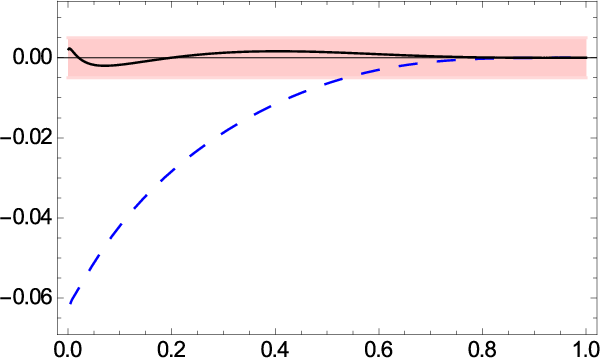
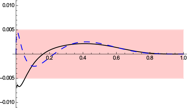
The remaining terms δ​Hinv(3±)​(x)\delta H^{(3\pm)}_{\rm inv}(x) contain the whole algebraic complexity of the full result but numerically they are rather small. For illustration we show the ratio δ​Hinv(3+)​(x)/Hinv(3+)​(x)\delta H^{(3+)}_{\rm inv}(x)/H^{(3+)}_{\rm inv}(x) for Nc=3N_{c}=3 and nf=4n_{f}=4 in Fig. 1 (dashed blue curve on the left panel). One sees that δ​Hinv(3+)​(x)\delta H^{(3+)}_{\rm inv}(x) contributes at most 6%6\% to the full splitting function in the whole range 0<x<10<x<1 so that for all practical purposes it can be approximated by a simple expression with a few parameters.

Refer to caption
Refer to caption
Figure 1: Left panel shows the ratio δ​Hinv(3+)​(x)/Hinv(3+)​(x)\delta H^{(3+)}_{\rm inv}(x)/H^{(3+)}_{\rm inv}(x) (dashed curve) for exact splitting functions and the error in using the approximation (68), (δ​Hinv(3+)|fit−δ​Hinv(3+)|exact)/Hinv(3+)(\delta H^{(3+)}_{\rm inv}|_{\rm fit}-\delta H^{(3+)}_{\rm inv}|_{\rm exact})/H^{(3+)}_{\rm inv} (solid curve) for nf=4n_{f}=4. The shaded area indicates an error band of 0.5%0.5\%. The similarly defined approximation error for the combinations H(+)+H(−)H^{(+)}+H^{(-)} (dashes) and H(+)−H(−)H^{(+)}-H^{(-)} (solid) which give rise to moments with odd and even NN, respectively, is shown on the right panel.

Due to the reciprocity property (58) the functions δ​Hinv(3±)​(x)\delta H^{(3\pm)}_{\rm inv}(x) can be parameterized in the form

δ​Hinv(3±)​(x)=x¯​h±​(x/x¯2).\displaystyle\delta H^{(3\pm)}_{\rm inv}(x)=\bar{x}\,h_{\pm}(x/\bar{x}^{2})\,. (67)

We choose the following ansatz

h±​(t)=H0±​a±t+a±​(1+b±​tt+a±),\displaystyle h_{\pm}(t)=H^{\pm}_{0}\frac{a_{\pm}}{t+a_{\pm}}\left(1+\frac{b_{\pm}\,t}{t+a_{\pm}}\right)\,, (68)

where a±a_{\pm} and b±b_{\pm} are fit parameters and the normalization constants H0±H_{0}^{\pm} are determined analytically from the condition δ​Hinv(3±)​(x)​=x→0​H0±+𝒪⁡(x)\delta H_{\rm inv}^{(3\pm)}(x)\underset{x\to 0}{=}H_{0}^{\pm}+\mathcal{O}(x) (64). The fitted values of the parameters a±a_{\pm} and b±b_{\pm} for the different color structures can be found in Table 2. With this simple parametrization we reduce the deviation from the exact splitting functions to less than 0.5%, see Fig. 1.

H0+H_{0}^{+} a+a_{+} b+b_{+}
CF3C_{F}^{3} 2723−28​π29−64​π445\dfrac{272}{3}-\dfrac{28\pi^{2}}{9}-\dfrac{64\pi^{4}}{45} 0.22630.2263 00
CF2​nfC_{F}^{2}n_{f} 323−16​π29\dfrac{32}{3}-\dfrac{16\pi^{2}}{9} 0.53400.5340 00
CF2Nc\dfrac{C_{F}^{2}}{N_{c}} −368​ζ33−9929+176​π29+4​π49-\dfrac{368\zeta_{3}}{3}-\dfrac{992}{9}+\dfrac{176\pi^{2}}{9}+\dfrac{4\pi^{4}}{9} 0.051740.05174 4.1164.116
CF​nfNc\dfrac{C_{F}n_{f}}{N_{c}} −32​ζ33+2569−8​π29-\dfrac{32\zeta_{3}}{3}+\dfrac{256}{9}-\dfrac{8\pi^{2}}{9} 0.096260.09626 −1.526-1.526
CF2Nc2\dfrac{C_{F}^{2}}{N^{2}_{c}} −328​ζ33−7369+140​π29+8​π45-\dfrac{328\zeta_{3}}{3}-\dfrac{736}{9}+\dfrac{140\pi^{2}}{9}+\dfrac{8\pi^{4}}{5} 0.065950.06595 00
H0−H_{0}^{-} a−a_{-} b−b_{-}
CF2Nc\dfrac{C_{F}^{2}}{N_{c}} 128​ζ3−24−2200​π227+28​π49128\zeta_{3}-24-\dfrac{2200\pi^{2}}{27}+\dfrac{28\pi^{4}}{9} 0.40400.4040 −0.7986-0.7986
CF​nfNc\dfrac{C_{F}n_{f}}{N_{c}} 176​π227−16​ζ3\dfrac{176\pi^{2}}{27}-16\zeta_{3} 0.12520.1252 00
CF2Nc2\dfrac{C_{F}^{2}}{N^{2}_{c}} 64​ζ3−24−1208​π227+7​π4964\zeta_{3}-24-\dfrac{1208\pi^{2}}{27}+\dfrac{7\pi^{4}}{9} 0.22060.2206 −1.077-1.077
Table 2: Values of the parameters in the ansatz for δ​Hinv(3±)​(x)\delta H^{(3\pm)}_{\rm inv}(x) (67), (68).

5.2 Mellin transformation

The following Mellin representation of the kernels χinv​(τ)\chi_{\rm inv}(\tau) and χinvℙ​(τ)\chi_{\rm inv}^{\mathbb{P}}(\tau) proves to be useful in order to restore them from the splitting functions and allows one to write all terms in the form that automatically respects the reciprocity relation:

χ⁡(τ)\displaystyle\chi(\tau) =12​π​i​∫c−i​∞c+i​∞d​ρ​χ~​(ρ)​(τ¯/τ)−ρ,\displaystyle=\frac{1}{2\pi i}\int_{c-i\infty}^{c+i\infty}\,d\rho\,\widetilde{\chi}(\rho)\left({\bar{\tau}}/{\tau}\right)^{-\rho}\,, (69a)
χ~​(ρ)\displaystyle\widetilde{\chi}(\rho) =∫01d​ττ​τ¯​(τ¯/τ)ρ​χ​(τ).\displaystyle=\int_{0}^{1}\frac{d\tau}{\tau\bar{\tau}}\left(\bar{\tau}/\tau\right)^{\rho}\,\chi(\tau)\,. (69b)

The integration contour in the first integral, (69a), must be chosen in the analyticity strip of the second integral, (69b), (the strip where integral converges). Making use of this representation one obtains

Δ​γinv(3+)​(N)\displaystyle\Delta\gamma_{\rm inv}^{(3+)}(N) =12​π​i​∫c−i​∞c+i​∞d​ρ​χ~inv(3)​(ρ)​Γ2​(1+ρ)​Γ⁡(jN−1−ρ)Γ⁡(jN+1+ρ),\displaystyle=\frac{1}{2\pi i}\int_{c-i\infty}^{c+i\infty}\,d\rho\,\widetilde{\chi}^{(3)}_{\rm inv}(\rho)\Gamma^{2}(1+\rho)\frac{\Gamma(j_{N}-1-\rho)}{\Gamma(j_{N}+1+\rho)}\,, (70a)
γinv(3−)​(N)\displaystyle\gamma_{\rm inv}^{(3-)}(N) =12​π​i​∫c−i​∞c+i​∞d​ρ​χ~invℙ⁡(3)​(ρ)​Γ2​(1+ρ)​Γ⁡(jN−1−ρ)Γ⁡(jN+1+ρ).\displaystyle=\frac{1}{2\pi i}\int_{c-i\infty}^{c+i\infty}\,d\rho\,\widetilde{\chi}^{\mathbb{P}(3)}_{\rm inv}(\rho)\Gamma^{2}(1+\rho)\frac{\Gamma(j_{N}-1-\rho)}{\Gamma(j_{N}+1+\rho)}. (70b)

Since for large jNj_{N} the ratio Γ⁡(jN−1−ρ)/Γ⁡(jN+1+ρ)∼jN−2​(1+ρ)\Gamma(j_{N}-1-\rho)/{\Gamma(j_{N}+1+\rho)}\sim j_{N}^{-2(1+\rho)}, the asymptotic expansion of the integrals in Eqs. (70) at jN→∞j_{N}\to\infty can be obtained by moving the integration contour to the right and picking up the corresponding residues. It is easy to check that if the only singularities of the Mellin-transformed kernels χ~​(ρ)\widetilde{\chi}(\rho) in the right half-plane are poles (of arbitrary order) at real integer values of ρ\rho, then a generic term of the asymptotic expansion of the anomalous dimensions has the form

(ψ⁡(jN)−ψ⁡(1))m(jN​(jN−1))k,k>0,m≥0,\frac{(\psi(j_{N})-\psi(1))^{m}}{(j_{N}(j_{N}-1))^{k}},\qquad k>0,m\geq 0\,,

which is required by the reciprocity symmetry under the jN↦1−jNj_{N}\mapsto 1-j_{N} transformation [18, 19, 20]. Under the same condition (χ~​(ρ)\widetilde{\chi}(\rho) only has poles at integer ρ\rho values in the right half-plane), the kernels χ⁡(τ)\chi(\tau) at small values of the conformal ratio have the expansion

χ⁡(τ)=∑k​mck​m​τk​lnm​τ.\chi(\tau)=\sum_{km}c_{km}\tau^{k}\ln^{m}\tau\,.

The Mellin transform of the one-loop kernel is very simple:

χinv(1)=−4CF↔χ~inv(1)=−4CF[2πiδ(ρ)].\displaystyle\chi_{\rm inv}^{(1)}=-4C_{F}\qquad\leftrightarrow\qquad\widetilde{\chi}_{\rm inv}^{(1)}=-4C_{F}\Big[2\pi i\delta(\rho)\Big]\,. (71)

More examples are collected in Table A, see App. A. One finds that the Mellin space kernels have a rather simple form, while the corresponding anomalous dimensions can be quite involved. Also the two-loop evolution kernels in Mellin space are given by rather compact expressions, see Eq. (A.119).

If the anomalous dimensions are written in terms of the splitting functions, Eq. (56),

γinv(k±)(N)=−∫01dxxNHinv(k±)(x),\displaystyle\gamma_{\rm inv}^{(k\pm)}(N)=-\int_{0}^{1}dx\,x^{N}H_{\rm inv}^{(k\pm)}(x)\,, (72)

the corresponding Mellin-transformed invariant kernels can be calculated as

χ~inv(k)​(ρ)\displaystyle\widetilde{\chi}_{\rm inv}^{(k)}(\rho) =−Γ⁡(2​ρ+2)Γ2​(1+ρ)∫01dxHinv(k+)(x)1x​x¯(1+x1−x)(xx¯2)ρ\displaystyle=-\frac{\Gamma(2\rho+2)}{\Gamma^{2}(1+\rho)}\int_{0}^{1}dx\,H_{\rm inv}^{(k+)}(x)\,\frac{1}{x\bar{x}}\left(\frac{1+x}{1-x}\right)\left(\frac{x}{\bar{x}^{2}}\right)^{\rho}\, (73)

and similar for χ~invℙ⁡(k)​(ρ)\widetilde{\chi}_{\rm inv}^{\mathbb{P}(k)}(\rho), with the replacement Hinv(k+)​(x)→Hinv(k−)​(x)H_{\rm inv}^{(k+)}(x)\to H_{\rm inv}^{(k-)}(x). The kernels in τ\tau space can finally be obtained by the inverse Mellin transformation (69a). We found this two-step approach to be the most effective for the three-loop case.

For the remainder function δ​Hinv(3±)​(x)\delta H^{(3\pm)}_{\rm inv}(x) written in the form (67) one obtains in Mellin space

δχ~inv(3±)(ρ)=−Γ⁡(2​ρ+2)Γ2​(1+ρ)∫0∞dth±(t)tρ−1,\displaystyle\delta\widetilde{\chi}^{(3\pm)}_{\rm inv}(\rho)=-\frac{\Gamma(2\rho+2)}{\Gamma^{2}(1+\rho)}\int_{0}^{\infty}dt\,h_{\pm}(t)\,t^{\rho-1}\,, (74)

and for the simple ansatz in Eq. (68)

δ​χ~inv(3±)​(ρ)\displaystyle\delta\widetilde{\chi}^{(3\pm)}_{\rm inv}(\rho) =−Γ⁡(2​ρ+2)Γ2​(1+ρ)​πsin⁡(π​ρ)​H0±​(1+b±​ρ)​a±ρ.\displaystyle=-\frac{\Gamma(2\rho+2)}{\Gamma^{2}(1+\rho)}\frac{\pi}{\sin(\pi\rho)}H^{\pm}_{0}(1+b_{\pm}\rho)a_{\pm}^{\rho}\,. (75)

Using Eq. (69a) we finally obtain the following expression for the corresponding contribution to the invariant kernel

δ​χinv(3±)​(τ)=H0±(1+4​a±​τ/τ¯)5/2​[1+a±​ττ¯​(4−6​b±)]−H0±.\displaystyle\delta{\chi}^{(3\pm)}_{\rm inv}(\tau)=\frac{H^{\pm}_{0}}{\left(1+4a_{\pm}\tau/\bar{\tau}\right)^{5/2}}\left[1+a_{\pm}\frac{\tau}{\bar{\tau}}(4-6\,b_{\pm})\right]-H^{\pm}_{0}\,. (76)

We also need the expressions for the functions ϕk\phi_{k} (60) in ρ\rho- and τ\tau-space defined as

ϕ~k​(ρ)\displaystyle\widetilde{\phi}_{k}(\rho) ≡−Γ⁡(2​ρ+2)Γ2​(1+ρ)∫01dxϕk(x)1x​x¯(1+x1−x)(xx¯2)ρ≡∫01d​ττ​τ¯(τ¯/τ)ρφk(τ).\displaystyle\equiv-\frac{\Gamma(2\rho+2)}{\Gamma^{2}(1+\rho)}\int_{0}^{1}dx\,\phi_{k}(x)\,\frac{1}{x\bar{x}}\left(\frac{1+x}{1-x}\right)\left(\frac{x}{\bar{x}^{2}}\right)^{\rho}\equiv\int_{0}^{1}\frac{d\tau}{\tau\bar{\tau}}\left(\bar{\tau}/\tau\right)^{\rho}\,\varphi_{k}(\tau)\,. (77)

One obtains

ϕ~1​(ρ)\displaystyle\widetilde{\phi}_{1}(\rho) =−π/(ρsinπρ),\displaystyle=-{\pi}/(\rho\sin\pi\rho),
ϕ~2​(ρ)\displaystyle\widetilde{\phi}_{2}(\rho) =ϕ~1​(ρ)​ρ¯ρ,\displaystyle=\widetilde{\phi}_{1}(\rho)\,\frac{\bar{\rho}}{\rho},
ϕ~3​(ρ)\displaystyle\widetilde{\phi}_{3}(\rho) =ϕ~1​(ρ)​(−2​ρ¯ρ+ψ′​(ρ)−π26),\displaystyle=\widetilde{\phi}_{1}(\rho)\,\Big(-2\,\frac{\bar{\rho}}{\rho}+\psi^{\prime}(\rho)-\frac{\pi^{2}}{6}\Big),
ϕ~4​(ρ)\displaystyle\widetilde{\phi}_{4}(\rho) =ϕ~1​(ρ)​(5​ρ¯ρ+(1−3​ρ)ρ​[ψ′​(ρ)−π26]),\displaystyle=\widetilde{\phi}_{1}(\rho)\,\Big(5\,\frac{\bar{\rho}}{\rho}+\frac{(1-3\rho)}{\rho}\Big[\psi^{\prime}(\rho)-\frac{\pi^{2}}{6}\Big]\Big), (78)

and

φ1​(τ)\displaystyle\varphi_{1}(\tau) =ln⁡τ¯=H1​(−ττ¯),\displaystyle=\ln\bar{\tau}=H_{1}\left(-\frac{\tau}{\bar{\tau}}\right)\,,
φ2​(τ)\displaystyle\varphi_{2}(\tau) =−φ1(τ)+H01(−ττ¯)=−lnτ¯+Li2(−τ/τ¯),\displaystyle=-\varphi_{1}(\tau)+H_{01}\left(-\frac{\tau}{\bar{\tau}}\right)=-\ln\bar{\tau}+\Li_{2}\left(-\tau/\bar{\tau}\right)\,,
φ3​(τ)\displaystyle\varphi_{3}(\tau) =−2​φ2​(x)−H101​(−ττ¯)=2​H1​(−ττ¯)−2​H01​(−ττ¯)−H101​(−ττ¯),\displaystyle=-2\varphi_{2}(x)-H_{101}\left(-\frac{\tau}{\bar{\tau}}\right)=2H_{1}\left(-\frac{\tau}{\bar{\tau}}\right)-2H_{01}\left(-\frac{\tau}{\bar{\tau}}\right)-H_{101}\left(-\frac{\tau}{\bar{\tau}}\right)\,,
=2lnτ¯−2Li2(−τ/τ¯)−2(Li3(τ¯)−Li3(1))+lnτ¯(Li2(τ¯)+π26)+16ln3τ¯\displaystyle=2\ln\bar{\tau}-2\Li_{2}\left(-\tau/\bar{\tau}\right)-2\Big(\Li_{3}(\bar{\tau})-\Li_{3}(1)\Big)+\ln\bar{\tau}\left(\Li_{2}(\bar{\tau})+\frac{\pi^{2}}{6}\right)+\frac{1}{6}\ln^{3}\bar{\tau}
φ4​(τ)\displaystyle\varphi_{4}(\tau) =−3​φ3​(τ)−φ2​(τ)−H0101​(−ττ¯)\displaystyle=-3\varphi_{3}(\tau)-\varphi_{2}(\tau)-H_{0101}\left(-\frac{\tau}{\bar{\tau}}\right)
=−5​H1​(−ττ¯)+5​H01​(−ττ¯)+3​H101​(−ττ¯)−H0101​(−ττ¯),\displaystyle=-5H_{1}\left(-\frac{\tau}{\bar{\tau}}\right)+5H_{01}\left(-\frac{\tau}{\bar{\tau}}\right)+3H_{101}\left(-\frac{\tau}{\bar{\tau}}\right)-H_{0101}\left(-\frac{\tau}{\bar{\tau}}\right), (79)

where Hp​…​q​(z)H_{p\ldots q}(z) are harmonic polylogarithms, see Ref. [29].

With these expressions at hand, our result for the invariant kernel (47) is complete. We obtain

χinv(3)​(τ)\displaystyle\chi_{\rm inv}^{(3)}(\tau) =∑k=14Bk(3+)​φk​(τ)−C0(3+)+C1(3+)​[ln⁡(τ/τ¯)+2]+δ​χinv(3+)​(τ),\displaystyle=\sum_{k=1}^{4}B^{(3+)}_{k}\varphi_{k}(\tau)-C^{(3+)}_{0}+C^{(3+)}_{1}\big[\ln\left(\tau/\bar{\tau}\right)+2\big]+\delta{\chi}^{(3+)}_{\rm inv}(\tau)\,,
χinvℙ⁡(3)​(τ)\displaystyle\chi_{\rm inv}^{\mathbb{P}(3)}(\tau) =∑k=14Bk(3−)​φk​(τ)−C0(3−)+δ​χinv(3−)​(τ),\displaystyle=\sum_{k=1}^{4}B^{(3-)}_{k}\varphi_{k}(\tau)-C^{(3-)}_{0}+\delta{\chi}^{(3-)}_{\rm inv}(\tau)\,, (80)

where the functions φk​(τ)\varphi_{k}(\tau) are defined in Eq. (79), the coefficients Bk(3±)B^{(3\pm)}_{k}, Ck(3±)C^{(3\pm)}_{k} can be found in Table 1 and the parameters for δ​χinv(3±)​(τ)\delta{\chi}^{(3\pm)}_{\rm inv}(\tau) (76) are collected in Table 2.

For illustration, in Fig. 2 we compare the full NNLO invariant functions χ⁡(a)=a​χ(1)+a2​χ(2)+a3​χ(3)\chi(a)=a\chi^{(1)}+a^{2}\chi^{(2)}+a^{3}\chi^{(3)} with the NLO, 𝒪⁡(a2)\mathcal{O}(a^{2}), and the LO, 𝒪⁡(a)\mathcal{O}(a), results for a typical value of the coupling αs/π=0.1\alpha_{s}/\pi=0.1 and, for definiteness, nf=4n_{f}=4. In the same plot the NNLO results using the exact three-loop functions obtained by the numerical integration of Eq. (54) are shown by dots. One sees that the accuracy of our parametrization is rather good. The remaining entries in the invariant kernel are, for the same values nf=4n_{f}=4 and αs/π=0.1\alpha_{s}/\pi=0.1,

Γcusp\displaystyle\Gamma_{\rm cusp} =a​Γ(1)​(1+8.019​a+80.53​a2+…)=a​Γ(1)​(1+0.2005+0.0503+…),\displaystyle=a\Gamma^{(1)}(1+8.019a+80.53a^{2}+\ldots)=a\Gamma^{(1)}(1+0.2005+0.0503+\ldots)\,,
χ0\displaystyle\chi_{0} =a​χ0(1)​(1−0.7935​a−141.3​a2+…)=a​χ0(1)​(1−0.0198−0.0883+…).\displaystyle=a\chi_{0}^{(1)}(1-0.7935a-141.3a^{2}+\ldots)=a\chi_{0}^{(1)}(1-0.0198-0.0883+\ldots)\,. (81)
Refer to caption ⁢ χ inv ( τ ) τ
Refer to caption ⁢ χ inv P ( τ ) τ
Figure 2: Invariant functions χinv​(τ)\chi_{\rm inv}(\tau) (left panel) and χinvℙ​(τ)\chi_{\rm inv}^{\mathbb{P}}(\tau) (right panel) for αs/π=0.1\alpha_{s}/\pi=0.1. The LO result (short dashes) is shown together with the NLO (long dashes) and NNLO (solid curves). The NNLO results using exact 𝒪⁡(a3)\mathcal{O}(a^{3}) functions obtained by the numerical integration of Eq. (54) are shown by black dots for comparison.

6 From light-ray to local operators

Light-ray operators are nothing but the generating functions for the renormalized local operators so that the mixing matrices for flavor-nonsinglet local operators can be calculated, in principle, by evaluating the evolution kernels on the test functions of the form f⁡(z1,z2)=z1m​z2kf(z_{1},z_{2})=z_{1}^{m}z_{2}^{k}, cf. (2). The results in this form are required for several applications, e.g. the calculation of moments of the distribution amplitudes and generalized nucleon parton distributions using lattice QCD techniques where the precision is increasing steadily and in some case already now requires NNLO accuracy [5].

Instead of using mixing matrices for the operators with a given number of left and right derivatives, as in Eq. (2), it proves to be more convenient to go over to the Gegenbauer polynomial basis. To the leading-order accuracy these operators diagonalize the evolution equations. Apart from convenience, writing the results in this form will allow us to make explicit connection to the formalism and notations used in [13] where the NLO expressions have been presented in this basis. We will see that the local operator formalism has its own advantages, e.g., solving the conformal constraint (21) is significantly easier in this language. Also the final step, reconstructing the invariant kernels from the eigenvalues, can be completely avoided here, as they directly enter the anomalous dimension matrices as diagonal elements.

Our goal is to translate the evolution kernels for light-ray operators into the anomalous dimension matrices for local operators of the form

𝒪n​k\displaystyle\mathcal{O}_{nk} =(∂z1+∂z2)kCn3/2(∂z1−∂z2∂z1+∂z2)𝒪(z1,z2)|z1=z2=0,k≥n.\displaystyle=(\partial_{z_{1}}+\partial_{z_{2}})^{k}C_{n}^{3/2}\left(\frac{\partial_{z_{1}}-\partial_{z_{2}}}{\partial_{z_{1}}+\partial_{z_{2}}}\right)\mathcal{O}(z_{1},z_{2})\bigg|_{z_{1}=z_{2}=0}\,,\qquad k\geq n\,. (82)

Here kk is the total number of derivatives and the operator of the lowest dimension for given nn, 𝒪n≡𝒪n​n\mathcal{O}_{n}\equiv\mathcal{O}_{nn}, is a conformal operator (lowest weight of the representation of the S​L​(2)SL(2) group). Increasing kk for fixed nn corresponds to adding total derivatives.

The operators 𝒪n​k\mathcal{O}_{nk} mix under the evolution

(μ∂∂μ+β(a)∂∂a)[𝒪n​k]=−∑n′=0nγn​n′[𝒪n′​k].\displaystyle\left(\mu\frac{\partial}{\partial\mu}+\beta(a)\frac{\partial}{\partial a}\right)[\mathcal{O}_{nk}]=-\sum_{n^{\prime}=0}^{n}\gamma_{nn^{\prime}}\,[\mathcal{O}_{n^{\prime}k}]\,. (83)

The mixing matrix γn​n′\gamma_{nn^{\prime}} is triangular and its diagonal elements are equal to the anomalous dimensions

γn​n′=0ifn′>n,\displaystyle\gamma_{nn^{\prime}}=0\quad\text{if}\quad n^{\prime}>n\,, γn​n=γn.\displaystyle\gamma_{nn}=\gamma_{n}\,. (84)

Since γn​n′\gamma_{nn^{\prime}} does not depend on kk, the second subscript kk is essentially redundant. In what follows we will use a “hat” for the anomalous dimensions and other quantities in matrix notation

𝜸^≡γn​n′.\displaystyle\widehat{\boldsymbol{\gamma}}\equiv\gamma_{nn^{\prime}}\,. (85)

The light-ray operator (2) can be expanded in terms of the local operators defined in Eq. (82)

𝒪⁡(x,z1,z2)=∑n=0∞∑k=n∞Φn​k​(z1,z2)​𝒪n​k​(x),\displaystyle\mathcal{O}(x;z_{1},z_{2})=\sum_{n=0}^{\infty}\sum_{k=n}^{\infty}\Phi_{nk}(z_{1},z_{2})\mathcal{O}_{nk}(x)\,, (86)

where the coefficients Φn​k​(z1,z2)\Phi_{nk}(z_{1},z_{2}) are homogeneous polynomials of two variables of degree kk [30]:

Φn​k​(z1,z2)=ωn​k​(S+(0))k−n​z12n,\displaystyle\Phi_{nk}(z_{1},z_{2})=\omega_{nk}(S_{+}^{(0)})^{k-n}z_{12}^{n}\,, ωn​k=2​2​n+3(k−n)!​Γ⁡(n+2)Γ⁡(n+k+4).\displaystyle\omega_{nk}=2\frac{2n+3}{(k-n)!}\frac{\Gamma(n+2)}{\Gamma(n+k+4)}\,. (87)

These polynomials are mutually orthogonal and form a complete set of functions33 3 Our notation in this section is adapted to facilitate the comparison with Ref. [13] and differs from the notation used in [30]. In particular the functions Φn​k\Phi_{nk} defined in (87) correspond to Φn,k−n\Phi_{n,k-n} in  [30]. w.r.t. the canonical S​L​(2)SL(2) scalar product (see, e.g., [30])

⟨Φn​k|Φn′​k′⟩=δk​k′​δn​n′​‖Φn​k‖2=δk​k′​δn​n′​ωn​k​ρn−1,\displaystyle\langle\Phi_{nk}|\Phi_{n^{\prime}k^{\prime}}\rangle=\delta_{kk^{\prime}}\delta_{nn^{\prime}}||\Phi_{nk}||^{2}=\delta_{kk^{\prime}}\delta_{nn^{\prime}}\,\omega_{nk}\rho_{n}^{-1}\,, ρn=12​(n+1)​(n+2)!\displaystyle\rho_{n}=\frac{1}{2}{(n+1)(n+2)!} (88)

so that the local operators (82) can be obtained by the projection on the corresponding “state”

𝒪n​k\displaystyle\mathcal{O}_{nk} =ρn​ωn​k−1​⟨Φn​k|𝒪⁡(z1,z2)⟩=ρn​⟨(S+)k−n​z12n|𝒪⁡(z1,z2)⟩.\displaystyle=\rho_{n}\omega_{nk}^{-1}\langle\Phi_{nk}|\mathcal{O}(z_{1},z_{2})\rangle=\rho_{n}\langle\left(S_{+}\right)^{k-n}z_{12}^{n}|\mathcal{O}(z_{1},z_{2})\rangle\,. (89)

The (canonical) conformal spin generators S±(0)S^{(0)}_{\pm} act as rising and lowering operators on this space whereas S0(0CLOSES^{(0}_{0} is diagonal

S0(0)​Φn​k​(z1,z2)=\displaystyle S_{0}^{(0)}\Phi_{nk}(z_{1},z_{2})= (k+2)​Φn​k​(z1,z2),\displaystyle~(k+2)\Phi_{nk}(z_{1},z_{2})\,,
S+(0)​Φn​k​(z1,z2)=\displaystyle S_{+}^{(0)}\Phi_{nk}(z_{1},z_{2})= (k−n+1)​(n+k+4)​Φn​k+1​(z1,z2),\displaystyle~(k-n+1)(n+k+4)\Phi_{nk+1}(z_{1},z_{2})\,,
S−(0)​Φn​k​(z1,z2)=\displaystyle S_{-}^{(0)}\Phi_{nk}(z_{1},z_{2})= −Φn​k−1​(z1,z2).\displaystyle~-\Phi_{nk-1}(z_{1},z_{2})\,. (90)

Thus the set of coefficient functions Φn,k​(z1,z2)\Phi_{n,k}(z_{1},z_{2}) for k={n​…​∞}k=\{n\ldots\infty\} forms an irreducible representation of the S​L​(2)SL(2) algebra, which is usually referred to as the conformal tower.

Let 𝒜\mathcal{A} be a certain operator 𝒜\mathcal{A} acting on quantum fields. Its action can be realized by the expansion in terms of local operators with “matrix elements” serving as expansion coefficients

[𝒜,𝒪n​k]=∑n′​k′An​n′k​k′​𝒪n′​k′.\displaystyle[\mathcal{A},\mathcal{O}_{nk}]=\sum_{n^{\prime}k^{\prime}}A_{nn^{\prime}}^{kk^{\prime}}\,\mathcal{O}_{n^{\prime}k^{\prime}}\,. (91)

Alternatively one can represent 𝒜\mathcal{A} by some integro-differential operator 𝐀{\bf A} acting on the arguments z1,z2z_{1},z_{2} of the light-ray operator 𝒪⁡(z1,z2)\mathcal{O}(z_{1},z_{2}) and, by means of the expansion (86), on the coefficient functions,

[𝒜,O]​(z1,z2)=∑n​kΦn​k​(z1,z2)​∑n′​k′An​n′k​k′​𝒪n′​k′≡[𝐀​O]​(z1,z2)=∑n​k[𝐀​Φn​k]​(z1,z2)​On​k.\displaystyle[\mathcal{A},O](z_{1},z_{2})=\sum_{nk}\Phi_{nk}(z_{1},z_{2})\sum_{n^{\prime}k^{\prime}}A_{nn^{\prime}}^{kk^{\prime}}\,\mathcal{O}_{n^{\prime}k^{\prime}}~\equiv~[{\bf A}O](z_{1},z_{2})=\sum_{nk}[{\bf A}\Phi_{nk}](z_{1},z_{2})O_{nk}\,. (92)

Comparing the representations in Eqs. (91) and (92) we see that the action of 𝐀{\bf A} on the coefficient functions of local operators is given by the transposed matrix

[𝐀​Φn​k]​(z1,z2)=∑n′​k′An′​nk′​k​Φn′​k′​(z1,z2).\displaystyle[{\bf A}\Phi_{nk}](z_{1},z_{2})=\sum_{n^{\prime}k^{\prime}}A_{n^{\prime}n}^{k^{\prime}k}\Phi_{n^{\prime}k^{\prime}}(z_{1},z_{2})\,. (93)

Using the orthogonality relation (88) one obtains

An​n′k​k′=‖Φn​k‖−2​⟨Φn​k​(z1,z2)|[𝐀​Φn′​k′]​(z1,z2)⟩≡⟨n​k​|𝐀|​n′​k′⟩,\displaystyle A_{nn^{\prime}}^{kk^{\prime}}=||\Phi_{nk}||^{-2}\langle\Phi_{nk}(z_{1},z_{2})|[{\bf A}\Phi_{n^{\prime}k^{\prime}}](z_{1},z_{2})\rangle~\equiv~\langle{nk}|{\bf A}|{n^{\prime}k^{\prime}}\rangle\,, (94)

which is the desired conversion, for a generic operator, between the light-ray and local operator representations.

The “matrix elements” An​n′k​k′A_{nn^{\prime}}^{kk^{\prime}} depend in general on four indices. However, if the operator 𝐀\bf A has a certain (canonical) dimension, i.e [S0(0),𝐀]=d𝐀​𝐀[S^{(0)}_{0},{\bf A}]=d_{\bf A}\bf A, then its matrix elements are nonzero only if the indices satisfy the constraint d𝐀=k−k′d_{\bf A}=k-k^{\prime}. This reduces the number of independent indices by one and allows one to write An​n′k​k′≡An​n′​(k)​δk,k′+d𝐀A_{nn^{\prime}}^{kk^{\prime}}\equiv A_{nn^{\prime}}(k)\delta_{k,k^{\prime}+d_{\bf A}}. If, in addition, the operator 𝒜\mathcal{A} is invariant under translations, i.e. [S−,𝐀]=0[S_{-},{\bf A}]=0, then it follows from Eqs. (90) that the matrix elements An​n′k​k′≡An​n′A_{nn^{\prime}}^{kk^{\prime}}\equiv A_{nn^{\prime}} do not depend on the upper indices at all.

Constraints on the operator mixing in the light-ray operator representation that follow from conformal algebra take the form (21)

[S+(0),ℍ⁡(a)]\displaystyle\big[S_{+}^{(0)},\mathbb{H}(a)\big] =[ℍ⁡(a),z1+z2]​(β¯​(a)+12​ℍ​(a))+[ℍ⁡(a),z12​Δ​(a)].\displaystyle=\big[\mathbb{H}(a),z_{1}+z_{2}\big]\left(\bar{\beta}(a)+\frac{1}{2}\mathbb{H}(a)\right)+\big[\mathbb{H}(a),z_{12}\Delta(a)\big]. (95)

To translate this equation into the local operator representation, we define the matrices

𝐚m​n​(k)\displaystyle\mathbf{a}_{mn}(k) =⟨m,k​|S+(0)|​n,k−1⟩,\displaystyle=\langle m,k|S_{+}^{(0)}|n,k-1\rangle\,,
𝐛m​n​(k)\displaystyle\mathbf{b}_{mn}(k) =⟨m,k​|z1+z2|​n,k−1⟩,\displaystyle=\langle m,k|z_{1}+z_{2}|n,k-1\rangle\,,
𝜸m​n\displaystyle\boldsymbol{\gamma}_{mn} =⟨m,k​|ℍ|​n,k⟩,\displaystyle=\langle m,k|\mathbb{H}|n,k\rangle\,,
𝐰m​n\displaystyle\mathbf{w}_{mn} =⟨m,k​|z12​Δ|​n,k−1⟩.\displaystyle=\langle m,k|z_{12}\Delta|n,k-1\rangle\,. (96)

The first two matrix elements are easily computed,

𝐚m​n​(k)\displaystyle\mathbf{a}_{mn}(k) =−(m−k)​(m+k+3)​δm​n≡−𝐚⁡(m,k)​δm​n,\displaystyle=-(m-k)(m+k+3)\delta_{mn}\equiv-{\bf a}(m,k)\delta_{mn}\,,
𝐛m​n​(k)\displaystyle\mathbf{b}_{mn}(k) =2​(k−n)​δm​n−2​(2​n+3)​ϑm​n,\displaystyle=2(k-n)\delta_{mn}-2(2n+3)\vartheta_{mn}\,, (97)

where we introduced a discrete step function

ϑm​n={1​ if ​m−n>0​ and even0​ else.\displaystyle\vartheta_{mn}=\begin{cases}1\text{ if }m-n>0\text{ and even}\\ 0\text{ else.}\end{cases}

The remaining two are nontrivial and can be written as a perturbative expansion

𝜸^​(a)\displaystyle\widehat{\boldsymbol{\gamma}}(a) =a​𝜸^(1)+a2​𝜸^(2)+a3​𝜸^(3)+…,a=αs4​π.\displaystyle=a\widehat{\boldsymbol{\gamma}}^{(1)}+a^{2}\widehat{\boldsymbol{\gamma}}^{(2)}+a^{3}\widehat{\boldsymbol{\gamma}}^{(3)}+\ldots\,,\qquad a=\frac{\alpha_{s}}{4\pi}\,.
𝐰^​(a)\displaystyle\widehat{\mathbf{w}}(a) =a​𝐰^(1)+a2​𝐰^(2)+….\displaystyle=a\widehat{\mathbf{w}}^{(1)}+a^{2}\widehat{\mathbf{w}}^{(2)}+\ldots\,. (98)

Eq. (95) becomes in matrix notation

[𝐚^,𝜸^​(a)]=[𝜸^​(a),𝐛^]​(β¯​(a)+12​𝜸^​(a))+[𝜸^,𝐰^​(a)].\displaystyle[\widehat{\bf a},\widehat{\boldsymbol{\gamma}}(a)]=[\widehat{\boldsymbol{\gamma}}(a),\widehat{\bf b}]\left(\bar{\beta}(a)+\frac{1}{2}\widehat{\boldsymbol{\gamma}}(a)\right)+[\widehat{\boldsymbol{\gamma}},\widehat{\bf w}(a)]\,. (99)

Note that the matrices 𝐚^​(k)\widehat{\bf a}(k) and 𝐛^​(k){\widehat{\bf b}}(k) (97) depend in principle on the total number of derivatives kk. However, due to the fact that only diagonal elements depend on this parameter, the dependence on kk drops out in the commutator. Hence we can safely omit it.

In complete analogy to the light-ray operator formulation, this equation fixes the non-diagonal (i.e. canonically non-invariant) part of the anomalous dimension matrix. Indeed, the commutator on the l.h.s. of Eq. (99) takes the form

[𝐚^,𝜸^​(a)]m​n\displaystyle[\widehat{\bf a},\widehat{\boldsymbol{\gamma}}(a)]_{mn} =(−𝐚⁡(m,k)+𝐚⁡(n,k))​γm​n=−𝐚⁡(m,n)​γm​n,\displaystyle=(-\mathbf{a}(m,k)+\mathbf{a}(n,k))\gamma_{mn}=-\mathbf{a}(m,n)\gamma_{mn}\,, (100)

so that the non-diagonal elements of the mixing matrix are given by [8]

𝜸^ND​(a)=𝒢⁡{[𝜸^​(a),𝐛^]​(12​𝜸^​(a)+β¯​(a))+[𝜸^​(a),𝐰^​(a)]},\displaystyle\widehat{\boldsymbol{\gamma}}^{\text{ND}}(a)=\mathcal{G}\left\{[\widehat{\boldsymbol{\gamma}}(a),\widehat{\bf b}]\left(\frac{1}{2}\widehat{\boldsymbol{\gamma}}(a)+\bar{\beta}(a)\right)+[\widehat{\boldsymbol{\gamma}}(a),\widehat{\bf w}(a)]\right\}, (101)

where

𝒢​{M^}m​n=−Mm​n𝐚⁡(m,n).\displaystyle\mathcal{G}\big\{\widehat{M}\big\}_{mn}=-\frac{M_{mn}}{{\bf a}(m,n)}\,. (102)

In particular to the two-loop accuracy

𝜸^(2),ND=𝒢⁡{[𝜸^(1),𝐛^]​(12​𝜸^(1)+β0)+[𝜸^(1),𝐰^(1)]}.\displaystyle\widehat{\boldsymbol{\gamma}}^{(2),\text{ND}}=\mathcal{G}\left\{[\widehat{\boldsymbol{\gamma}}^{(1)},\widehat{\bf b}]\left(\frac{1}{2}\widehat{\boldsymbol{\gamma}}^{(1)}+\beta_{0}\right)+[\widehat{\boldsymbol{\gamma}}^{(1)},\widehat{\bf w}^{(1)}]\right\}. (103)

Here 𝜸^(1)\widehat{\boldsymbol{\gamma}}^{(1)} is the well-known (diagonal) matrix of one-loop anomalous dimensions

γm​n(1)\displaystyle{\gamma}_{mn}^{(1)} =γn(1)​δm​n=2​δm​n​CF​(4​S1​(n+1)−2(n+1)​(n+2)−3)\displaystyle=\gamma^{(1)}_{n}\delta_{mn}=2\delta_{mn}C_{F}\big(4S_{1}(n+1)-\frac{2}{(n+1)(n+2)}-3\big) (104)

and 𝐰^(1)\widehat{\bf w}^{(1)} is the one-loop conformal anomaly

𝐰m​n(1)\displaystyle{\bf w}_{mn}^{(1)} =4​CF​(2​n+3)​𝐚​(m,n)​(Am​n−S1​(m+1)(n+1)​(n+2)+2​Am​n𝐚⁡(m,n))​ϑm​n,\displaystyle=4C_{F}(2n+3)\,\mathbf{a}(m,n)\left(\frac{A_{mn}-S_{1}(m+1)}{(n+1)(n+2)}+\frac{2A_{mn}}{\mathbf{a}(m,n)}\right)\vartheta_{mn}\,, (105)

where

Am​n=S1​(m+n+22)−S1​(m−n−22)+2​S1​(m−n−1)−S1​(m+1).\displaystyle A_{mn}=S_{1}\left(\frac{m+n+2}{2}\right)-S_{1}\left(\frac{m-n-2}{2}\right)+2S_{1}(m-n-1)-S_{1}(m+1). (106)

Collecting everything one obtains the two-loop anomalous dimension matrix:

γm​n(2)\displaystyle\gamma^{(2)}_{mn} =δm​n​γn(2)−γm(1)−γn(1)𝐚⁡(m,n)​{−2​(2​n+3)​(β0+12​γn(1))​ϑm​n+𝐰m​n(1)}.\displaystyle=\delta_{mn}\gamma^{(2)}_{n}-\frac{\gamma^{(1)}_{m}-\gamma^{(1)}_{n}}{\mathbf{a}(m,n)}\biggl\{-2(2n+3)\left(\beta_{0}+\frac{1}{2}\gamma^{(1)}_{n}\right)\vartheta_{mn}+{\bf w}_{mn}^{(1)}\biggr\}. (107)

The first few elements (0≤n≤7,0≤m≤7)(0\leq n\leq 7,~0\leq m\leq 7) for Nc=3N_{c}=3 are

γm​n(2)\displaystyle{\gamma}_{mn}^{(2)} =(0000000002348824300000026090344502430000008668243052419143037500005290851224306628463375000012069285050261232787508336325438587500−205414175034243202502208998708750718751707308700000226526357210982399551250732074225004705570987512032250423000)\displaystyle=\begin{pmatrix}0&0&0&0&0&0&0&0\\ 0&\frac{23488}{243}&0&0&0&0&0&0\\ \frac{260}{9}&0&\frac{34450}{243}&0&0&0&0&0\\ 0&\frac{8668}{243}&0&\frac{5241914}{30375}&0&0&0&0\\ \frac{52}{9}&0&\frac{8512}{243}&0&\frac{662846}{3375}&0&0&0\\ 0&\frac{120692}{8505}&0&\frac{261232}{7875}&0&\frac{83363254}{385875}&0&0\\ -\frac{2054}{14175}&0&\frac{34243}{2025}&0&\frac{2208998}{70875}&0&\frac{718751707}{3087000}&0\\ 0&\frac{226526}{35721}&0&\frac{982399}{55125}&0&\frac{7320742}{250047}&0&\frac{557098751203}{2250423000}\end{pmatrix}
−nf​(00000000051281000000409083081000000882702654220250000104450106440503113220250000114456702321050171247699225004108283502421350180494503745727198450002372170105063150286017010362419431786050).\displaystyle\hskip 28.45274pt-n_{f}\begin{pmatrix}0&0&0&0&0&0&0&0\\ 0&\frac{512}{81}&0&0&0&0&0&0\\ \frac{40}{9}&0&\frac{830}{81}&0&0&0&0&0\\ 0&\frac{88}{27}&0&\frac{26542}{2025}&0&0&0&0\\ \frac{104}{45}&0&\frac{1064}{405}&0&\frac{31132}{2025}&0&0&0\\ 0&\frac{1144}{567}&0&\frac{232}{105}&0&\frac{1712476}{99225}&0&0\\ \frac{4108}{2835}&0&\frac{242}{135}&0&\frac{1804}{945}&0&\frac{3745727}{198450}&0\\ 0&\frac{2372}{1701}&0&\frac{506}{315}&0&\frac{2860}{1701}&0&\frac{36241943}{1786050}\\ \end{pmatrix}. (108)

Our expressions for the one-loop conformal anomaly and the two-loop anomalous dimension matrix coincide identically with the results in [13].44 4 The explicit relation to the notations in [13] is as follows: 𝐚^​(k)|[13]=−12​𝐚^​(k)\widehat{\mathbf{a}}(k)|_{\text{\cite[cite]{\@@bibref{Authors Phrase1YearPhrase2}{Belitsky:1998gc}{\@@citephrase{(}}{\@@citephrase{)}}}}}=-\frac{1}{2}\widehat{\mathbf{a}}(k), 𝐛^​(k)|[13]=𝐛^​(k)\widehat{\mathbf{b}}(k)|_{\text{\cite[cite]{\@@bibref{Authors Phrase1YearPhrase2}{Belitsky:1998gc}{\@@citephrase{(}}{\@@citephrase{)}}}}}=\widehat{\mathbf{b}}(k), 𝐰^(1)|[13]=−𝐰^(1)\widehat{\mathbf{w}}^{(1)}|_{\text{\cite[cite]{\@@bibref{Authors Phrase1YearPhrase2}{Belitsky:1998gc}{\@@citephrase{(}}{\@@citephrase{)}}}}}=-\widehat{\mathbf{w}}^{(1)}, and γ^[13](i)=2i​γ^(i−1)\widehat{\gamma}^{(i)}_{\text{\cite[cite]{\@@bibref{Authors Phrase1YearPhrase2}{Belitsky:1998gc}{\@@citephrase{(}}{\@@citephrase{)}}}}}=2^{i}\widehat{\gamma}^{(i-1)}. A perturbative expansion in [13] is done in powers of αs/(2​π)\alpha_{s}/(2\pi), e.g., 𝜸^​(a)=∑i(2​a)i​𝜸^(i−1)\widehat{\boldsymbol{\gamma}}(a)=\sum_{i}(2a)^{i}\widehat{\boldsymbol{\gamma}}^{(i-1)}.

Expanding Eq. (101) to the third order, we obtain the three-loop nondiagonal anomalous dimension matrix in the form

𝜸^(3),ND=𝒢⁡{[𝜸^(2),𝐛^]​(12​𝜸^(1)+β0)+[𝜸^(2),𝐰^(1)]+[𝜸^(1),𝐛^]​(12​𝜸^(2)+β1)+[𝜸^(1),𝐰^(2)]}.\displaystyle\widehat{\boldsymbol{\gamma}}^{(3),\text{ND}}=\mathcal{G}\bigg\{[\widehat{\boldsymbol{\gamma}}^{(2)},\widehat{\bf b}](\frac{1}{2}\widehat{\boldsymbol{\gamma}}^{(1)}+\beta_{0})+[\widehat{\boldsymbol{\gamma}}^{(2)},\widehat{\bf w}^{(1)}]+[\widehat{\boldsymbol{\gamma}}^{(1)},\widehat{\bf b}](\frac{1}{2}\widehat{\boldsymbol{\gamma}}^{(2)}+\beta_{1})+[\widehat{\boldsymbol{\gamma}}^{(1)},\widehat{\bf w}^{(2)}]\bigg\}\,. (109)

In addition to the already known quantities, this expression involves the matrix element of the two-loop conformal anomaly (B.126),

𝐰m​n(2)=⟨m,k​|z12​Δ(2)|​n,k−1⟩=14​[𝜸^(2),𝐛^]+Δ​𝐰m​n(2)\displaystyle\mathbf{w}_{mn}^{(2)}=\langle m,k|z_{12}\Delta^{(2)}|n,k-1\rangle=\frac{1}{4}[\widehat{\boldsymbol{\gamma}}^{(2)},\widehat{\mathbf{b}}]+\Delta{\bf w}_{mn}^{(2)} (110)

where

Δ​𝐰m​n(2)=⟨m,k​|z12​Δ+(2)|​n,k−1⟩.\displaystyle\Delta{\bf w}_{mn}^{(2)}=\langle m,k|z_{12}\Delta_{+}^{(2)}|n,k-1\rangle\,. (111)

The explicit expression for the operator Δ+(2)\Delta_{+}^{(2)} (B.127) can be found in [16]. We have not found a closed analytic expression for the matrix Δ​𝐰m​n(2)\Delta{\bf w}_{mn}^{(2)}, but the values for given m,nm,n can be evaluated in a straightforward way.

Splitting the result into different color structures,

Δ​𝐰^(2)=CF2​Δ​𝐰^P+CFNc​Δ​𝐰^F​A+β0​CF​Δ​𝐰^b​F,\displaystyle\Delta\widehat{\bf w}^{(2)}=C_{F}^{2}\Delta\widehat{\bf w}^{P}+\frac{C_{F}}{N_{c}}\Delta\widehat{\bf w}^{FA}+\beta_{0}C_{F}\Delta\widehat{\bf w}^{bF},

we get for the first few elements (0≤n≤5,1≤m≤7)(0\leq n\leq 5,~1\leq m\leq 7)

Δ​𝐰^F​A=\displaystyle\Delta\widehat{\bf w}^{FA}= (000000−754000000−50751080000−679150−587237200000−7399900−724339600000−1070777168000−12001960−12335709175600000−229746772116800−1015076275880000−3083848691481760),\displaystyle\begin{pmatrix}0&0&0&0&0&0\\ -\frac{75}{4}&0&0&0&0&0\\ 0&-\frac{5075}{108}&0&0&0&0\\ -\frac{679}{15}&0&-\frac{58723}{720}&0&0&0\\ 0&-\frac{7399}{90}&0&-\frac{724339}{6000}&0&0\\ -\frac{1070777}{16800}&0&-\frac{12001}{96}&0&-\frac{123357091}{756000}&0\\ 0&-\frac{22974677}{211680}&0&-\frac{101507627}{588000}&0&-\frac{308384869}{1481760}\\ \end{pmatrix},
Δ​𝐰^P=\displaystyle\Delta\widehat{\bf w}^{P}= (000000−2965144000000−1176553108000000−14095990000−7387709360000000−752083916174000−2111899581686000000−6837234354880000−5045910661211680000−30745779392974088000000−999113242938001504000−80893123457922226400000−29426151034675601052800),\displaystyle\begin{pmatrix}0&0&0&0&0&0\\ -\frac{2965}{144}&0&0&0&0&0\\ 0&-\frac{1176553}{10800}&0&0&0&0\\ -\frac{140959}{9000}&0&-\frac{7387709}{36000}&0&0&0\\ 0&-\frac{75208391}{617400}&0&-\frac{2111899581}{6860000}&0&0\\ -\frac{68372343}{5488000}&0&-\frac{5045910661}{21168000}&0&-\frac{307457793929}{740880000}&0\\ 0&-\frac{99911324293}{800150400}&0&-\frac{808931234579}{2222640000}&0&-\frac{2942615103467}{5601052800}\\ \end{pmatrix},
Δ​𝐰^b​F=\displaystyle\Delta\widehat{\bf w}^{bF}= (00000035000000185527000010520255524000028913001468391000006459100039031327000255240713500002028291764047983132450001436501361740).\displaystyle\begin{pmatrix}0&0&0&0&0&0\\ 35&0&0&0&0&0\\ 0&\frac{1855}{27}&0&0&0&0\\ \frac{105}{2}&0&\frac{2555}{24}&0&0&0\\ 0&\frac{2891}{30}&0&\frac{146839}{1000}&0&0\\ \frac{6459}{100}&0&\frac{390313}{2700}&0&\frac{2552407}{13500}&0\\ 0&\frac{202829}{1764}&0&\frac{4798313}{24500}&0&\frac{14365013}{61740}\\ \end{pmatrix}. (112)

Using these expressions and the diagonal matrix elements from [6] we obtain the full three-loop anomalous dimension matrix

𝜸^(3)=diag⁡{γ0(3),γ1(3),…}+𝜸^⟨1⟩(3)+nf​𝜸^⟨nf⟩(3)+nf2​𝜸^⟨nf2⟩(3),\displaystyle\widehat{\boldsymbol{\gamma}}^{(3)}={\rm diag}\{\gamma_{0}^{(3)},\gamma_{1}^{(3)},\ldots\}+\widehat{\boldsymbol{\gamma}}^{(3)}_{\langle 1\rangle}+n_{f}\,\widehat{\boldsymbol{\gamma}}^{(3)}_{\langle n_{f}\rangle}+n_{f}^{2}\,\widehat{\boldsymbol{\gamma}}^{(3)}_{\langle n_{f}^{2}\rangle}\,, (113)

where the off-diagonal matrices for Nc=3N_{c}=3 and different powers of nfn_{f} in the range 0≤n≤7,0≤m≤70\leq n\leq 7,~0\leq m\leq 7 are given by the following expressions:

𝜸^⟨1⟩(3)\displaystyle\widehat{\boldsymbol{\gamma}}^{(3)}_{\langle 1\rangle} =(000000000000000049024810000000036623912546750000003911270235998913645000000080493047233125587503206579817315209312500000281851388261750141000002080521942477144200000218982695060473750705000000007192640196053567106596000159898280729473525098700000022002377525170939697461720000),\displaystyle=\begin{pmatrix}0&0&0&0&0&0&0&0\\ 0&0&0&0&0&0&0&0\\ \frac{49024}{81}&0&0&0&0&0&0&0\\ 0&\frac{36623912}{54675}&0&0&0&0&0&0\\ \frac{3911}{27}&0&\frac{23599891}{36450}&0&0&0&0&0\\ 0&\frac{8049304723}{31255875}&0&\frac{320657981731}{520931250}&0&0&0&0\\ \frac{281851388261}{7501410000}&0&\frac{208052194247}{714420000}&0&\frac{21898269506047}{37507050000}&0&0&0\\ 0&\frac{7192640196053}{56710659600}&0&\frac{159898280729473}{525098700000}&0&\frac{220023775251709}{396974617200}&0&0\\ \end{pmatrix},
𝜸^⟨nf⟩(3)\displaystyle\widehat{\boldsymbol{\gamma}}^{(3)}_{\langle n_{f}\rangle} =(0000000000000000−2870024300000000−576218854675000000−1279108303750−26434828273375000000−849255644187535250−51607766857881250000−5494282725004700−636248861133953750−775078310719376762500000−1660976917675126900−74961724611562793750−3640609352947258883000),\displaystyle=\begin{pmatrix}0&0&0&0&0&0&0&0\\ 0&0&0&0&0&0&0&0\\ -\frac{28700}{243}&0&0&0&0&0&0&0\\ 0&-\frac{5762188}{54675}&0&0&0&0&0&0\\ -\frac{1279108}{30375}&0&-\frac{26434828}{273375}&0&0&0&0&0\\ 0&-\frac{849255644}{18753525}&0&-\frac{516077668}{5788125}&0&0&0&0\\ -\frac{54942827}{2500470}&0&-\frac{636248861}{13395375}&0&-\frac{77507831071}{937676250}&0&0&0\\ 0&-\frac{1660976917}{67512690}&0&-\frac{7496172461}{156279375}&0&-\frac{36406093529}{472588830}&0&0\\ \end{pmatrix},
𝜸^⟨nf2⟩(3)\displaystyle\widehat{\boldsymbol{\gamma}}^{(3)}_{\langle n_{f}^{2}\rangle} =(00000000000000002368100000000317212150000001316202504135618225000000187412178605022012110250000551698930250107939450017653999225000072619316074450681503595350051535932148900).\displaystyle=\begin{pmatrix}0&0&0&0&0&0&0&0\\ 0&0&0&0&0&0&0&0\\ \frac{236}{81}&0&0&0&0&0&0&0\\ 0&\frac{3172}{1215}&0&0&0&0&0&0\\ \frac{1316}{2025}&0&\frac{41356}{18225}&0&0&0&0&0\\ 0&\frac{187412}{178605}&0&\frac{22012}{11025}&0&0&0&0\\ \frac{55169}{893025}&0&\frac{10793}{9450}&0&\frac{176539}{99225}&0&0&0\\ 0&\frac{726193}{1607445}&0&\frac{681503}{595350}&0&\frac{515359}{321489}&0&0\end{pmatrix}. (114)

For completeness we also write the first few anomalous dimensions [6]:

γ0(3)=\displaystyle\gamma^{(3)}_{0}= 0,\displaystyle 0\,,
γ1(3)=\displaystyle\gamma^{(3)}_{1}= 256081​ζ3+110284166561−(256027​ζ3+3344002187)​nf−1792729​nf2,\displaystyle\frac{2560}{81}\zeta_{3}+\frac{11028416}{6561}-\left(\frac{2560}{27}\zeta_{3}+\frac{334400}{2187}\right)n_{f}-\frac{1792}{729}n_{f}^{2}\,,
γ2(3)=\displaystyle\gamma_{2}^{(3)}= 220081​ζ3+6448619926244−(400027​ζ3+9674954374)​nf−2569729​nf2,\displaystyle\frac{2200}{81}\zeta_{3}+\frac{64486199}{26244}-\left(\frac{4000}{27}\zeta_{3}+\frac{967495}{4374}\right)n_{f}-\frac{2569}{729}n_{f}^{2}\,,
γ3(3)=\displaystyle\gamma_{3}^{(3)}= 11512405​ζ3+24578790565182012500−(502427​ζ3+7265912712733750)​nf−38427791125​nf2,\displaystyle\frac{11512}{405}\zeta_{3}+\frac{245787905651}{82012500}-\left(\frac{5024}{27}\zeta_{3}+\frac{726591271}{2733750}\right)n_{f}-\frac{384277}{91125}n_{f}^{2}\,,
γ4(3)=\displaystyle\gamma_{4}^{(3)}= 11312405​ζ3+559048023977164025000−(582427​ζ3+90842989303750)​nf−43124291125​nf2,\displaystyle\frac{11312}{405}\zeta_{3}+\frac{559048023977}{164025000}-\left(\frac{5824}{27}\zeta_{3}+\frac{90842989}{303750}\right)n_{f}-\frac{431242}{91125}n_{f}^{2}\,,
γ5(3)=\displaystyle\gamma_{5}^{(3)}= 55889619845​ζ3+103373346851366872756768175000−(45376189​ζ3+7138103329432187911250)​nf−16069514231255875​nf2,\displaystyle\frac{558896}{19845}\zeta_{3}+\frac{10337334685136687}{2756768175000}-\left(\frac{45376}{189}\zeta_{3}+\frac{713810332943}{2187911250}\right)n_{f}-\frac{160695142}{31255875}n_{f}^{2}\,,
γ6(3)=\displaystyle\gamma_{6}^{(3)}= 1854826615​ζ3+5938857531795763914702763600000−(1643263​ζ3+1222518688750335006580000)​nf−1369936511250047000​nf2,\displaystyle\frac{185482}{6615}\zeta_{3}+\frac{59388575317957639}{14702763600000}-\left(\frac{16432}{63}\zeta_{3}+\frac{12225186887503}{35006580000}\right)n_{f}-\frac{1369936511}{250047000}n_{f}^{2}\,,
γ7(3)=\displaystyle\gamma_{7}^{(3)}= 5020814178605​ζ3+4602864819209954443110718314664400000−(158128567​ζ3+349136571992501945177660000)​nf−389209777976751269000​nf2.\displaystyle\frac{5020814}{178605}\zeta_{3}\!+\frac{46028648192099544431}{10718314664400000}-\!\left(\!\frac{158128}{567}\zeta_{3}\!+\!\frac{349136571992501}{945177660000}\!\right)n_{f}\!-\frac{38920977797}{6751269000}n_{f}^{2}\,. (115)

To visualize the size of the three-loop correction we consider the full NNLO nondiagonal part of the anomalous dimension matrix for nf=4n_{f}=4 in the same range (0≤n≤7,0≤m≤7)(0\leq n\leq 7,~0\leq m\leq 7):

𝜸^ND=a2​(000000000000000011.1+179​a0000000022.6+290​a000000−3.47−13.2​a024.5+297​a0000006.12+93.2​a024.3+291​a0000−5.94−49.3​a09.74+120​a023.5+282​a00000.0764+35.6​a011.4+131​a022.6+272​a00).\displaystyle\widehat{\boldsymbol{\gamma}}^{\rm ND}=a^{2}\begin{pmatrix}0&0&0&0&0&0&0&0\\ 0&0&0&0&0&0&0&0\\ 11.1+179a &0&0&0&0&0&0&0\\ 0&22.6+290a&0&0&0&0&0&0\\ -3.47-13.2a&0&24.5+297a&0&0&0&0&0\\ 0&6.12+93.2a&0&24.3+291a&0&0&0&0\\ -5.94-49.3a&0&9.74+120a&0&23.5+282a&0&0&0\\ 0&0.0764+35.6a&0&11.4+131a&0&22.6+272a&0&0\end{pmatrix}. (116)

For realistic values of the strong coupling a=αs/(4​π)∼1/40a=\alpha_{s}/(4\pi)\sim 1/40 the three-loop contribution is on the average about 30% of the two-loop result.

7 Conclusions

Using the two-loop result for the conformal anomaly obtained in Ref. [16] we have completed here the calculation of the three-loop evolution kernel for the flavor-nonsinglet leading-twist operators in off-forward kinematics. The result is presented in the form of the evolution equation for the relevant nonlocal light-ray operator. In addition we derive the explicit expression for the three-loop anomalous dimension matrix for the local operators of dimension D≤10D\leq 10, i.e., containing up to seven covariant derivatives. In the latter form, our result is directly applicable to the renormalization of meson distribution amplitudes and will be useful for lattice calculations of their first few moments.

Practical methods for the solution of the three-loop evolution equations in more general GPD kinematics still have to be developed. Our results can, in principle, be translated to the evolution equation for GPDs by a Fourier transformation, although algebraic complexities of this transformation may prohibit obtaining the analytic expressions. An alternative method using the Mellin transformation in the conformal spin [31, 32] is very attractive and it has become the standard tool in the NLO analysis of the DVCS [33, 34, 35] and deeply-virtual meson production [36, 37]. The extension of this technique to NNLO was considered in [33, 34, 35] in a special “conformal” renormalization scheme. The transformation to the conventional MS¯\overline{\text{MS}} scheme can be done using the results of our paper, but it remains to be seen whether this works in practice without major complications. The NNLO analysis of the DVCS data will, of course, require the extension of our results to flavor-singlet operators.

Acknowledgments

This study was supported by Deutsche Forschungsgemeinschaft (DFG) with the grants MO 1801/1-2 and SFB/TRR 55.

Appendices

Appendix A Two-loop invariant kernel

The two-loop constant term χ0(2)\chi_{0}^{(2)} and the functions χinv(2)​(τ)\chi_{\rm inv}^{(2)}(\tau), χinvℙ⁡(2)​(τ)\chi_{\rm inv}^{\mathbb{P}(2)}(\tau) in the invariant kernel (36) are given by the following expressions:

χ0(2)\displaystyle\chi_{0}^{(2)} =13​CF​{β0​(37−4​π2)+CF​(43−4​π2)+1Nc​(26−8​π2+72​ζ3)},\displaystyle=\frac{1}{3}C_{F}\biggl\{\beta_{0}\big(37-4\pi^{2}\big)+C_{F}\big(43-4\pi^{2}\big)+\frac{1}{N_{c}}\big(26-8\pi^{2}+72\zeta_{3}\big)\biggr\}\,, (A.117)

and

χinv(2)​(τ)\displaystyle\chi_{\rm inv}^{(2)}(\tau) =4​CF​{−113​β0+CF​[ln⁡τ¯−203+2​π23]−2Nc​(Li2⁡(τ)+12​ln2​τ¯−1τ​ln⁡τ¯−π26+53)},\displaystyle=4C_{F}\biggl\{-\frac{11}{3}\beta_{0}+C_{F}\left[\ln\bar{\tau}-\frac{20}{3}+\frac{2\pi^{2}}{3}\right]-\frac{2}{N_{c}}\left(\Li_{2}(\tau)+\frac{1}{2}\ln^{2}\bar{\tau}-\frac{1}{\tau}\ln\bar{\tau}-\frac{\pi^{2}}{6}+\frac{5}{3}\right)\biggr\}\,,
χinvℙ⁡(2)​(τ)\displaystyle\chi_{\rm inv}^{\mathbb{P}(2)}(\tau) =−4​CFNc​(ln2⁡τ¯−2​τ​ln⁡τ¯).\displaystyle=-\frac{4C_{F}}{N_{c}}\Big(\ln^{2}\bar{\tau}-2\tau\ln\bar{\tau}\Big)\,. (A.118)

The corresponding kernels in Mellin space take a rather simple form

χ~inv(2)​(ρ)\displaystyle\widetilde{\chi}_{\rm inv}^{(2)}(\rho) =4​CF​{r0​(2​π​i)​δ​(−i​ρ)−πρ​sin⁡π​ρ​(CF+2Nc​2​ρ+1ρ⁡(ρ+1))},\displaystyle=4C_{F}\biggl\{r_{0}(2\pi i)\delta(-i\rho)-\frac{\pi}{\rho\sin\pi\rho}\left(C_{F}+\frac{2}{N_{c}}\frac{2\rho+1}{\rho(\rho+1)}\right)\biggr\}\,,
χ~invℙ⁡(2)​(ρ)\displaystyle\widetilde{\chi}_{\rm inv}^{\mathbb{P}(2)}(\rho) =−8​CFNc​πρ​sin⁡π​ρ​(ρ−1)​S1​(ρ−1),\displaystyle=-\frac{8C_{F}}{N_{c}}\frac{\pi}{\rho\sin\pi\rho}(\rho-1)S_{1}(\rho-1)\,, (A.119)

where

r0=−113​β0+CF​[2​π23−203]−2Nc​(83−π26).\displaystyle r_{0}=-\frac{11}{3}\beta_{0}+C_{F}\left[\frac{2\pi^{2}}{3}-\frac{20}{3}\right]-\frac{2}{N_{c}}\left(\frac{8}{3}-\frac{\pi^{2}}{6}\right)\,. (A.120)

The following table of Mellin transforms in Tab. A is helpful to arrive at this representation:

χ⁡(τ)\chi(\tau) −1π​ρ​sin⁡(π​ρ)​χ~​(ρ)-\dfrac{1}{\pi}\rho\sin(\pi\rho)\widetilde{\chi}(\rho) γ⁡(N),n=N+1\gamma(N),\ \ n=N+1
ln⁡τ¯\ln\bar{\tau} 11 −1(n⁡(n+1))2-\dfrac{1}{(n(n+1))^{2}}
τ¯τ​ln⁡τ¯+1\dfrac{\bar{\tau}}{\tau}\ln\bar{\tau}+1 −ρρ+1-\dfrac{\rho}{\rho+1} 2​S3​(n)−2​ζ3+1n⁡(n+1)2S_{3}(n)-2\zeta_{3}+\dfrac{1}{n(n+1)}
τ¯​ln⁡τ¯\bar{\tau}\ln\bar{\tau} ρ​S1​(ρ)\rho\,S_{1}(\rho) (−1)n​{2​S−3​(n)−4​S−2,1​(n)+2​S1​(n)​(2​S−2​(n)+π26)−ζ3}(-1)^{n}\biggl\{2S_{-3}(n)-4S_{-2,1}(n)+2S_{1}(n)\left(2S_{-2}(n)+\dfrac{\pi^{2}}{6}\right)-\zeta_{3}\biggr\}
12​ln2​τ¯\dfrac{1}{2}\ln^{2}\bar{\tau} S1​(ρ−1)S_{1}(\rho-1) n2+n+1n3​(n+1)3−(−1)nn⁡(n+1)​(2​S−2​(n)+π26)\dfrac{n^{2}+n+1}{n^{3}(n+1)^{3}}-\dfrac{(-1)^{n}}{n(n+1)}\left(2S_{-2}(n)+\dfrac{\pi^{2}}{6}\right)
Li2⁡(τ)\Li_{2}(\tau) −S1​(ρ)-S_{1}(\rho) (−1)nn⁡(n+1)​(2​S−2​(n)+π26)\dfrac{(-1)^{n}}{n(n+1)}\left(2S_{-2}(n)+\dfrac{\pi^{2}}{6}\right)
Table A: Mellin transformation (69) for several typical kernels and the corresponding contributions to the anomalous dimensions. Here S1​(ρ)=ψ⁡(ρ+1)−ψ⁡(1)S_{1}(\rho)=\psi(\rho+1)-\psi(1).

Appendix B 𝕏\mathbb{X} kernels

In this appendix we present explicit expressions for the kernels 𝕏(k)\mathbb{X}^{(k)} appearing in the operator of similarity transformation (24).

The one-loop kernel 𝕏(1)\mathbb{X}^{(1)} is defined as a solution to the differential equation (30a)

[S+(0),𝕏(1)]\displaystyle\big[S_{+}^{(0)},\mathbb{X}^{(1)}\big] =z12​Δ(1),\displaystyle=z_{12}\Delta^{(1)}\,, (B.121)

where Δ(1)\Delta^{(1)} is the 𝒪⁡(a)\mathcal{O}(a) conformal anomaly [15]

Δ(1)​f​(z1,z2)\displaystyle\Delta^{(1)}f(z_{1},z_{2}) =−2CF∫01dα(α¯α+lnα)[f(z12α,z2)−f(z1,z21α)].\displaystyle=-2C_{F}\int_{0}^{1}d\alpha\Big(\frac{\bar{\alpha}}{\alpha}+\ln\alpha\Big)\Big[f(z_{12}^{\alpha},z_{2})-f(z_{1},z_{21}^{\alpha})\Big]\,. (B.122)

The result reads

𝕏(1)​f​(z1,z2)\displaystyle\mathbb{X}^{(1)}f(z_{1},z_{2}) =2​CF​(∫01d​α​ln⁡αα​[2​f​(z1,z2)−f⁡(z12α,z2)−f⁡(z1,z21α)]+Δ​𝕏inv(1)),\displaystyle=2C_{F}\left(\int_{0}^{1}d\alpha\frac{\ln\alpha}{\alpha}\Big[2f(z_{1},z_{2})-f(z_{12}^{\alpha},z_{2})-f(z_{1},z_{21}^{\alpha})\Big]+\Delta\mathbb{X}^{(1)}_{\rm inv}\right)\,, (B.123)

where Δ​𝕏i​n​v(1)\Delta\mathbb{X}^{(1)}_{inv} is an invariant kernel (solution of the corresponding homogeneous equation) which has the following generic form (cf. (36)):

Δ​𝕏inv(1)​f​(z1,z2)\displaystyle\Delta\mathbb{X}^{(1)}_{\rm inv}f(z_{1},z_{2}) =X0​f​(z1,z2)+X1​∫01d​α​α¯α​(2​f​(z1,z2)−f⁡(z12α,z2)−f⁡(z1,z21α))\displaystyle=X_{0}f(z_{1},z_{2})+X_{1}\int_{0}^{1}d\alpha\frac{\bar{\alpha}}{\alpha}\Big(2f(z_{1},z_{2})-f(z_{12}^{\alpha},z_{2})-f(z_{1},z_{21}^{\alpha})\Big)
+∫01dα∫0α¯dβ(Δχ(τ)+ΔχP(τ)ℙ12)f(z12α,z21β).\displaystyle\quad+\int_{0}^{1}d\alpha\int_{0}^{\bar{\alpha}}d\beta\Big(\Delta\chi(\tau)+\Delta\chi_{P}(\tau)\mathbb{P}_{12}\Big)f(z_{12}^{\alpha},z_{21}^{\beta})\,. (B.124)

The choice of Δ​𝕏i​n​v(1)\Delta\mathbb{X}^{(1)}_{inv} is a matter of convenience, e.g., it can be put to zero.

The two-loop kernel 𝕏(2)\mathbb{X}^{(2)} is defined as a solution to Eq. (30b)

[S+(0),𝕏(2)]\displaystyle\big[S_{+}^{(0)},\mathbb{X}^{(2)}\big] =z12​Δ(2)+[𝕏(1),z1+z2]​(β0+12​ℍ(1))+12​[𝕏(1),z12​Δ(1)],\displaystyle=z_{12}\Delta^{(2)}+\Big[\mathbb{X}^{(1)},z_{1}+z_{2}\Big]\left(\beta_{0}+\frac{1}{2}\mathbb{H}^{(1)}\right)+\frac{1}{2}\Big[\mathbb{X}^{(1)},z_{12}\Delta^{(1)}\Big]\,, (B.125)

where [16]

z12​Δ(2)=z12​Δ+(2)+14​[ℍ(2),z1+z2].\displaystyle z_{12}\Delta^{(2)}=z_{12}\Delta^{(2)}_{+}+\frac{1}{4}\big[\mathbb{H}^{(2)},z_{1}+z_{2}\big]. (B.126)

The operator Δ+(2)\Delta^{(2)}_{+} takes the form

Δ+(2)​f​(z1,z2)\displaystyle\Delta_{+}^{(2)}f(z_{1},z_{2}) =∫01d​α​∫0α¯d​β​[ω⁡(α,β)+ωℙ​(α,β)​ℙ12]​[f⁡(z12α,z21β)−f⁡(z12β,z21α)]\displaystyle=\int_{0}^{1}\!d\alpha\!\int_{0}^{\bar{\alpha}}d\beta\Big[\omega(\alpha,\beta)+\omega^{\mathbb{P}}(\alpha,\beta)\mathbb{P}_{12}\Big]\Big[f(z_{12}^{\alpha},z_{21}^{\beta})-f(z_{12}^{\beta},z_{21}^{\alpha})\Big]
+∫01du∫01dtϰ(t)[f(z12u​t,z2)−f(z1,z21u​t)].\displaystyle\quad+\int_{0}^{1}\!du\int_{0}^{1}\!dt\,\varkappa(t)\,\Big[f(z_{12}^{ut},z_{2})-f(z_{1},z_{21}^{ut})\Big]. (B.127)

Explicit expressions for the functions ω⁡(α,β)\omega(\alpha,\beta), ωℙ​(α,β)\omega^{\mathbb{P}}(\alpha,\beta) and ϰ⁡(τ)\varkappa(\tau) can be found in [16] (see App. C2).

The solution can be written as a sum of three terms corresponding to the three contributions on the r.h.s. of Eq. (B.125),

𝕏(2)\displaystyle\mathbb{X}^{(2)} =𝕏I(2)+𝕏II(2)+𝕏III(2),\displaystyle=\mathbb{X}_{\rm I}^{(2)}+\mathbb{X}_{\rm II}^{(2)}+\mathbb{X}_{\rm III}^{(2)}, (B.128)

where

𝕏I(2)\displaystyle\mathbb{X}_{\rm I}^{(2)} =14​(𝕋(2)+β0​𝕋(2,1))+CF​(1−π26)​𝕋(1)+𝕏IA(2)+𝕏IB(2),\displaystyle=\frac{1}{4}\left(\mathbb{T}^{(2)}+\beta_{0}\mathbb{T}^{(2,1)}\right)+C_{F}\left(1-\frac{\pi^{2}}{6}\right)\mathbb{T}^{(1)}+\mathbb{X}_{\rm IA}^{(2)}+\mathbb{X}_{\rm IB}^{(2)}\,,
𝕏II(2)\displaystyle\mathbb{X}_{\rm II}^{(2)} =𝕏(2,1)​(β0+12​ℍ(1)),\displaystyle=\mathbb{X}^{(2,1)}\left(\beta_{0}+\frac{1}{2}\mathbb{H}^{(1)}\right)\,,
𝕏III(2)\displaystyle\mathbb{X}_{\rm III}^{(2)} =12​[Δ​𝕏i​n​v(1),𝕏(1)]−12​𝕏(2,2).\displaystyle=\frac{1}{2}\Big[\Delta\mathbb{X}_{inv}^{(1)},\mathbb{X}^{(1)}\Big]-\frac{1}{2}\mathbb{X}^{(2,2)}. (B.129)

The operators 𝕋(2)\mathbb{T}^{(2)}, 𝕋(2,1)\mathbb{T}^{(2,1)} are given in App. C and 𝕏(2,1)\mathbb{X}^{(2,1)}, 𝕏(2,2)\mathbb{X}^{(2,2)} are defined as solutions to the following equations:

[S+(0),𝕏(2,1)]=[𝕏(1),z1+z2],\displaystyle[S_{+}^{(0)},\mathbb{X}^{(2,1)}]=[\mathbb{X}^{(1)},z_{1}+z_{2}]\,, [S+(0),𝕏(2,2)]=[z12​Δ(1),𝕏(1)].\displaystyle[S_{+}^{(0)},\mathbb{X}^{(2,2)}]=[z_{12}\Delta^{(1)},\mathbb{X}^{(1)}]\,. (B.130)

One obtains

𝕏(2,1)​f​(z1,z2)\displaystyle\mathbb{X}^{(2,1)}f(z_{1},z_{2}) =2CF{−∫01dα(α¯α(1−X1)lnα¯+lnα)[2f(z1,z2)−f(z12α,z2)−f(z1,z21α)]\displaystyle=2C_{F}\biggl\{-\int_{0}^{1}d\alpha\left(\frac{\bar{\alpha}}{\alpha}(1-X_{1})\ln\bar{\alpha}+\ln\alpha\right)\Big[2f(z_{1},z_{2})-f(z_{12}^{\alpha},z_{2})-f(z_{1},z_{21}^{\alpha})\Big]
+∫01dα∫0α¯dβln(−α−β)(Δχ(τ)+ΔχP(τ)ℙ12)f(z12α,z21β)},\displaystyle\quad+\int_{0}^{1}d\alpha\int_{0}^{\bar{\alpha}}d\beta\,\ln(1\!-\!\alpha\!-\!\beta)\Big(\Delta\chi(\tau)+\Delta\chi_{P}(\tau)\mathbb{P}_{12}\Big)f(z_{12}^{\alpha},z_{21}^{\beta})\biggr\}\,, (B.131)

where X1X_{1}, Δ​χ​(τ)\Delta\chi(\tau), χP​(τ)\chi_{P}(\tau) are the entries in (B.124), and

𝕏(2,2)​f​(z1,z2)=\displaystyle\mathbb{X}^{(2,2)}f(z_{1},z_{2})= (B.132)
=\displaystyle= 4CF2{∫01dα∫01du[ln⁡α¯α(12lnα¯+2)+u¯uϑ⁡(α)α¯][2f(z1,z2)−f(z12α​u,z2)−f(z1,z21α​u)]\displaystyle 4C_{F}^{2}\biggl\{\int_{0}^{1}d\alpha\int_{0}^{1}du\left[\frac{\ln\bar{\alpha}}{\alpha}\left(\frac{1}{2}\ln\bar{\alpha}+2\right)+\frac{\bar{u}}{u}\frac{\vartheta(\alpha)}{\bar{\alpha}}\right]\Big[2f(z_{1},z_{2})-f(z_{12}^{\alpha u},z_{2})-f(z_{1},z_{21}^{\alpha u})\Big]
+∫01dα∫0α¯dβ[1τ(ϑ+(α)+ϑ+(β))[f(z12α,z21β)−f(z1,z21β)−f(z12α,z2)+f(z1,z2)]\displaystyle{}+\int_{0}^{1}d\alpha\int_{0}^{\bar{\alpha}}d\beta\biggl[\frac{1}{\tau}\Big(\vartheta_{+}(\alpha)+\vartheta_{+}(\beta)\Big)\Big[f(z_{12}^{\alpha},z_{21}^{\beta})-f(z_{1},z_{21}^{\beta})-f(z_{12}^{\alpha},z_{2})+f(z_{1},z_{2})\Big]
+(ϑ0(α)+ϑ0(β))f(z12α,z21β)]},\displaystyle{}\hskip 28.45274pt+\Big(\vartheta_{0}(\alpha)+\vartheta_{0}(\beta)\Big)f(z_{12}^{\alpha},z_{21}^{\beta})\biggr]\biggr\}\,,

where

ϑ+​(α)\displaystyle\vartheta_{+}(\alpha) =−1α¯​(ln⁡α​ln​α¯+2​α​ln​α+2​α¯​ln​α¯),\displaystyle=-\frac{1}{\bar{\alpha}}\Big(\ln\alpha\ln\bar{\alpha}+2\alpha\ln\alpha+2\bar{\alpha}\ln\bar{\alpha}\Big)\,,
ϑ0​(α)\displaystyle\vartheta_{0}(\alpha) =2​(Li3⁡(α¯)−Li3⁡(α)−ln⁡α¯​Li2⁡(α¯)+ln⁡α​Li2⁡(α))+1α​ln​α​ln​α¯+2α​ln​α¯,\displaystyle=2\Big(\Li_{3}(\bar{\alpha})-\Li_{3}(\alpha)-\ln\bar{\alpha}\,\Li_{2}(\bar{\alpha})+\ln\alpha\,\Li_{2}(\alpha)\Big)+\frac{1}{\alpha}\ln\alpha\ln\bar{\alpha}+\frac{2}{\alpha}\ln\bar{\alpha}\,, (B.133)
ϑ⁡(α)\displaystyle\vartheta(\alpha) =αα¯​(Li2⁡(α¯)−ln2⁡α)−12​α¯α​ln2​α¯+(α−2α)​ln​α​ln​α¯−(3+1α¯)​ln​α−(α−α¯)​α¯α​ln​α¯−2.\displaystyle=\frac{\alpha}{\bar{\alpha}}\Big(\Li_{2}(\bar{\alpha})-\ln^{2}\alpha\Big)-\frac{1}{2}\frac{\bar{\alpha}}{\alpha}\ln^{2}\bar{\alpha}+\left(\alpha-\frac{2}{\alpha}\right)\ln\alpha\ln\bar{\alpha}-\left(3+\frac{1}{\bar{\alpha}}\right)\ln\alpha-(\alpha-\bar{\alpha})\frac{\bar{\alpha}}{\alpha}\ln\bar{\alpha}-2\,.

The operators 𝕏IA(2)\mathbb{X}^{(2)}_{\rm IA}, 𝕏IB(2)\mathbb{X}^{(2)}_{\rm IB} which originate from the two-loop anomaly Δ+(2)\Delta^{(2)}_{+} are rather involved. We obtain

𝕏IA(2)​f​(z1,z2)\displaystyle\mathbb{X}^{(2)}_{\rm IA}f(z_{1},z_{2}) =∫01d​u​u¯u​∫01d​αα¯​[ϰ⁡(α)−ϰ⁡(1)]​[2​f​(z1,z2)−f⁡(z12α​u,z2)−f⁡(z1,z21α​u)]\displaystyle=\int_{0}^{1}\!du\,\frac{\bar{u}}{u}\int_{0}^{1}\frac{d\alpha}{\bar{\alpha}}\,\big[\varkappa(\alpha)-\varkappa(1)\big]\Big[2f(z_{1},z_{2})-f(z_{12}^{\alpha u},z_{2})-f(z_{1},z_{21}^{\alpha u})\Big]
+∫01dαξIA(α)[2f(z1,z2)−f(z12α,z2)−f(z1,z21α)],\displaystyle\quad+\int_{0}^{1}d\alpha\,\xi_{\rm IA}(\alpha)\Big[2f(z_{1},z_{2})-f(z_{12}^{\alpha},z_{2})-f(z_{1},z_{21}^{\alpha})\Big], (B.134)

where ϰ⁡(α)\varkappa(\alpha) is one of the functions entering the two-loop conformal anomaly (B.127) and

ξIA​(α)\displaystyle\xi_{\rm IA}(\alpha) =2CF2α¯α[−Li3(α¯)+lnα¯Li2(α¯)+13ln3α¯+Li2(α)+1α¯lnαlnα¯−14ln2α¯\displaystyle=2C_{F}^{2}\frac{\bar{\alpha}}{\alpha}\biggl[-\Li_{3}(\bar{\alpha})+\ln\bar{\alpha}\,\Li_{2}(\bar{\alpha})+\frac{1}{3}\ln^{3}\bar{\alpha}+\Li_{2}(\alpha)+\frac{1}{\bar{\alpha}}\ln\alpha\ln\bar{\alpha}-\frac{1}{4}\ln^{2}\bar{\alpha}
−3​αα¯lnα−3lnα¯]+CFNc(lnα+α¯αlnα¯).\displaystyle\quad-\frac{3\alpha}{\bar{\alpha}}\ln\alpha-3\ln\bar{\alpha}\biggr]+\frac{C_{F}}{N_{c}}\left(\ln\alpha+\frac{\bar{\alpha}}{\alpha}\ln\bar{\alpha}\right). (B.135)

Finally

𝕏IB(2)​f​(z1,z2)\displaystyle\mathbb{X}^{(2)}_{\rm IB}f(z_{1},z_{2}) =CF​∫01d​α​∫0α¯d​β​[CF​ξIBF​(α,β)+1Nc​(ξIBA​(α,β)+ξIBA​ℙ​(α,β)​ℙ12)]​f​(z12α,z21β),\displaystyle=C_{F}\int_{0}^{1}d\alpha\int_{0}^{\bar{\alpha}}d\beta\biggl[C_{F}\,\xi_{\rm IB}^{F}(\alpha,\beta)+\frac{1}{N_{c}}\Big(\xi_{\rm IB}^{A}\,(\alpha,\beta)+\xi_{\rm IB}^{A\mathbb{P}}(\alpha,\beta)\mathbb{P}_{12}\Big)\biggr]f(z_{12}^{\alpha},z_{21}^{\beta})\,, (B.136)

where

ξIBA​ℙ​(α,β)\displaystyle\xi_{\rm IB}^{A\mathbb{P}}(\alpha,\beta) =−2[Li3(α¯)−Li3(1−αβ¯)+1α¯[Li2(α)−Li2(αβ¯)]+lnτ¯Li2(1−αβ¯)\displaystyle=-2\biggl[\Li_{3}(\bar{\alpha})-\Li_{3}\left(1-\frac{\alpha}{\bar{\beta}}\right)+\frac{1}{\bar{\alpha}}\left[\Li_{2}(\alpha)-\Li_{2}\left(\frac{\alpha}{\bar{\beta}}\right)\right]+\ln\bar{\tau}\,\Li_{2}\left(1-\frac{\alpha}{\bar{\beta}}\right)
+1+α2​α¯lnα¯lnβ¯+(α↔β)],\displaystyle\quad+\frac{1+\alpha}{2\bar{\alpha}}\ln\bar{\alpha}\ln\bar{\beta}+(\alpha\leftrightarrow\beta)\biggr]\,,
ξIBA​(α,β)\displaystyle\xi_{\rm IB}^{A}(\alpha,\beta) =2[Li3(β¯)−2Li3(β)−Li3(1−βα¯)−Li3(βα¯)+lnτ¯Li2(1−βα¯)+ln(βα¯)Li2(β)\displaystyle=2\biggl[\Li_{3}(\bar{\beta})-2\Li_{3}(\beta)-\Li_{3}\left(1-\frac{\beta}{\bar{\alpha}}\right)-\Li_{3}\left(\frac{\beta}{\bar{\alpha}}\right)+\ln\bar{\tau}\,\Li_{2}\left(1-\frac{\beta}{\bar{\alpha}}\right)+\ln\left(\frac{\beta}{\bar{\alpha}}\right)\Li_{2}(\beta)
+1α(Li2(β)−Li2(βα¯))+2β¯βLi2(β)+12lnα¯lnβ¯+β¯βlnβlnβ¯+(α↔β)]\displaystyle\quad+\frac{1}{\alpha}\left(\Li_{2}(\beta)-\Li_{2}\left(\frac{\beta}{\bar{\alpha}}\right)\right)+2\frac{\bar{\beta}}{\beta}\Li_{2}(\beta)+\frac{1}{2}\ln\bar{\alpha}\ln\bar{\beta}+\frac{\bar{\beta}}{\beta}\ln\beta\ln\bar{\beta}+(\alpha\leftrightarrow\beta)\biggr] (B.137)

and

ξIBF​(α,β)\displaystyle\xi_{\rm IB}^{F}(\alpha,\beta) =ln⁡(1−α−β)​ln⁡(τ​τ¯)−13​ln3⁡(1−α−β)+3​ln​α¯​ln​β¯−ln⁡α​ln​β\displaystyle=\ln(1-\alpha-\beta)\ln(\tau\,\bar{\tau})-\frac{1}{3}\ln^{3}(1-\alpha-\beta)+3\ln\bar{\alpha}\ln\bar{\beta}-\ln\alpha\ln\beta
+[−6Li3(α¯)−10Li3(α)+2lnα¯Li2(α¯)+6lnαLi2(α)+lnαlnα¯(lnα+lnα¯−2)\displaystyle\quad+\biggl[-6\Li_{3}(\bar{\alpha})-10\Li_{3}(\alpha)+2\ln\bar{\alpha}\Li_{2}(\bar{\alpha})+6\ln\alpha\Li_{2}(\alpha)+\ln\alpha\ln\bar{\alpha}\big(\ln\alpha+\ln\bar{\alpha}-2\big)
−4​1+αα​(Li2⁡(α¯)−Li2⁡(1))−13​ln3​α¯−α¯α​ln2​α¯+12​ln2​α−2α¯​ln​α+4α​ln​α¯+15​ln​α¯\displaystyle\quad-4\frac{1+\alpha}{\alpha}\Big(\Li_{2}(\bar{\alpha})-\Li_{2}(1)\Big)-\frac{1}{3}\ln^{3}\bar{\alpha}-\frac{\bar{\alpha}}{\alpha}\ln^{2}\bar{\alpha}+\frac{1}{2}\ln^{2}\alpha-\frac{2}{\bar{\alpha}}\ln\alpha+\frac{4}{\alpha}\ln\bar{\alpha}+15\ln\bar{\alpha}
+(α↔β)].\displaystyle\quad+(\alpha\leftrightarrow\beta)\biggr]. (B.138)

In all expressions τ=α​βα¯​β¯\tau=\frac{\alpha\beta}{\bar{\alpha}\bar{\beta}}.

Appendix C 𝕋\mathbb{T} kernels

The 𝕋(k)\mathbb{T}^{(k)} operators, k=1,2,…k=1,2,\ldots are defined as solutions to the differential equation (33)

[S+(0),𝕋(k)]\displaystyle[S_{+}^{(0)},\mathbb{T}^{(k)}] =[𝐇inv(k),z1+z2],\displaystyle=[\mathbf{H}_{\rm inv}^{(k)},z_{1}+z_{2}], (C.139)

where 𝐇inv(k)\mathbf{H}_{\rm inv}^{(k)} are the S​L​(2)SL(2) invariant parts of the evolution kernel which have the general decomposition as shown in Eq. (36). This equation can easily be solved:

𝕋(k)​f​(z1,z2)\displaystyle\mathbb{T}^{(k)}f(z_{1},z_{2}) =−Γcusp(k)∫01dαα¯​ln⁡α¯α(f(z12α,z2)+f(z1,z21α))\displaystyle=-\Gamma_{\rm cusp}^{(k)}\int_{0}^{1}d\alpha\frac{\bar{\alpha}\ln\bar{\alpha}}{\alpha}\Big(f(z_{12}^{\alpha},z_{2})+f(z_{1},z_{21}^{\alpha})\Big)
+∫01dα∫0α¯dβln(1−α−β)(χinv(k)(τ)+χinvℙ⁡(k)(τ)ℙ12)f(z12α,z21β),\displaystyle\quad+\int_{0}^{1}d\alpha\int_{0}^{\bar{\alpha}}d\beta\ln(1-\alpha-\beta)\Big(\chi_{\rm inv}^{(k)}(\tau)+\chi_{\rm inv}^{\mathbb{P}(k)}(\tau)\mathbb{P}_{12}\Big)f(z_{12}^{\alpha},z_{21}^{\beta})\,, (C.140)

where the functions χinv(k)\chi_{\rm inv}^{(k)}, χinvℙ⁡(k)\chi_{\rm inv}^{\mathbb{P}(k)} for one loop, k=1k=1, and two loops, k=2k=2, are given in Eqs. (38) and (A.118), respectively.

The 𝕋1(2)\mathbb{T}^{(2)}_{1} kernel is defined as the solution to

[S+(0),𝕋1(2)]=[𝕋(1),z1+z2].\displaystyle[S_{+}^{(0)},\mathbb{T}^{(2)}_{1}]=[\mathbb{T}^{(1)},z_{1}+z_{2}]\,. (C.141)

Using the explicit expression for 𝕋(1)=𝐓inv(1)\mathbb{T}^{(1)}=\mathbf{T}_{\rm inv}^{(1)} (13) one obtains after a short calculation

𝕋1(2)​f​(z1,z2)\displaystyle\mathbb{T}^{(2)}_{1}f(z_{1},z_{2}) =−12∫01dαα¯​ln2​α¯α(f(z12α,z2)+f(z1,z21α))+12∫01dα∫0α¯dβln2(−α−β)f(z12α,z21β).\displaystyle=-\frac{1}{2}\int_{0}^{1}\!d\alpha\frac{\bar{\alpha}\ln^{2}\bar{\alpha}}{\alpha}\Big(f(z_{12}^{\alpha},z_{2})+f(z_{1},z_{21}^{\alpha})\Big)+\frac{1}{2}\int_{0}^{1}\!d\alpha\int_{0}^{\bar{\alpha}}\!d\beta\ln^{2}(1\!-\!\alpha\!-\!\beta)f(z_{12}^{\alpha},z_{21}^{\beta})\,. (C.142)

We stress again that Eqs. (33) determine the 𝕋\mathbb{T}-kernels up to the S​L​(2)SL(2) (canonically) invariant parts. Our choice in (C.140) and (C.142) corresponds to the following condition on the eigenvalues of these kernels: Let γinv(k)​(N)\gamma_{\rm inv}^{(k)}(N) be the eigenvalues of the invariant kernels 𝐇inv(k)\mathbf{H}_{\rm inv}^{(k)} (corresponding contributions to the anomalous dimensions),

𝐇inv(k)​z12N\displaystyle\mathbf{H}_{\rm inv}^{(k)}z_{12}^{N} =γinv(k)​(N)​z12N.\displaystyle=\gamma_{\rm inv}^{(k)}(N)z_{12}^{N}\,. (C.143)

It is easy to check that eigenvalues of the kernels defined in (C.140) and (C.142) are given by the following expressions:

𝕋(k)​z12N\displaystyle\mathbb{T}^{(k)}z_{12}^{N} =T(k)​(N)​z12N,T(k)​(N)=dd​N​γinv(k)​(N),\displaystyle={T}^{(k)}(N)z_{12}^{N}\,,\qquad{T}^{(k)}(N)=\frac{d}{dN}\gamma_{\rm inv}^{(k)}(N)\,,
𝕋1(2)​z12N\displaystyle\mathbb{T}_{1}^{(2)}z_{12}^{N} =T1(2)​(N)​z12N,T1(2)​(N)=12​d2d​N2​γinv(1)​(N).\displaystyle={T}_{1}^{(2)}(N)z_{12}^{N}\,,\qquad{T}_{1}^{(2)}(N)=\frac{1}{2}\frac{d^{2}}{dN^{2}}\gamma_{\rm inv}^{(1)}(N)\,. (C.144)

This choice is convenient for our present purposes as it leads to a certain symmetry of the three-loop invariant kernel 𝐇inv(3)\mathbf{H}_{\rm inv}^{(3)} that allows one to obtain somewhat simpler expressions, see Sec. 5.

References

  • (1) D. Boer et al., Gluons and the quark sea at high energies: Distributions, polarization, tomography, arXiv:1108.1713 [nucl-th].
  • (2) J. Dudek et al., Physics Opportunities with the 12 GeV Upgrade at Jefferson Lab, Eur. Phys. J. A 48 (2012) 187.
  • (3) T. Abe et al. [Belle-II Collaboration], Belle II Technical Design Report, arXiv:1011.0352 [physics.ins-det].
  • (4) A. Accardi et al., A Critical Appraisal and Evaluation of Modern PDFs, Eur. Phys. J. C 76 (2016) no.8, 471.
  • (5) V. M. Braun, S. Collins, M. Göckeler, P. Pérez-Rubio, A. Schäfer, R. W. Schiel and A. Sternbeck, Second Moment of the Pion Light-cone Distribution Amplitude from Lattice QCD, Phys. Rev. D 92 (2015) no.1, 014504.
  • (6) S. Moch, J. A. M. Vermaseren and A. Vogt, The Three loop splitting functions in QCD: The Nonsinglet case, Nucl. Phys. B 688 (2004) 101.
  • (7) D. Müller, Constraints for anomalous dimensions of local light cone operators in ϕ3\phi^{3} in six-dimensions theory, Z. Phys. C 49 (1991) 293.
  • (8) D. Müller, Conformal constraints and the evolution of the nonsinglet meson distribution amplitude, Phys. Rev. D 49 (1994) 2525.
  • (9) D. Müller, Restricted conformal invariance in QCD and its predictive power for virtual two photon processes, Phys. Rev. D 58 (1998) 054005.
  • (10) A. V. Belitsky and D. Müller, Predictions from conformal algebra for the deeply virtual Compton scattering, Phys. Lett. B 417 (1998) 129.
  • (11) A. V. Belitsky and D. Müller, Next-to-leading order evolution of twist-2 conformal operators: The Abelian case, Nucl. Phys. B 527 (1998) 207.
  • (12) A. V. Belitsky, A. Freund and D. Müller, Evolution kernels of skewed parton distributions: Method and two loop results, Nucl. Phys. B 574 (2000) 347.
  • (13) A. V. Belitsky and D. Müller, Broken conformal invariance and spectrum of anomalous dimensions in QCD, Nucl. Phys. B 537 (1999) 397.
  • (14) V. M. Braun and A. N. Manashov, Evolution equations beyond one loop from conformal symmetry, Eur. Phys. J. C 73 (2013) 2544.
  • (15) V. M. Braun and A. N. Manashov, Two-loop evolution equations for light-ray operators, Phys. Lett. B 734 (2014) 137.
  • (16) V. M. Braun, A. N. Manashov, S. Moch and M. Strohmaier, Two-loop conformal generators for leading-twist operators in QCD, JHEP 1603 (2016) 142.
  • (17) Y. L. Dokshitzer, G. Marchesini and G. P. Salam, Revisiting parton evolution and the large-x limit, Phys. Lett. B 634 (2006) 504.
  • (18) B. Basso and G. P. Korchemsky, Anomalous dimensions of high-spin operators beyond the leading order, Nucl. Phys. B 775 (2007) 1.
  • (19) L. F. Alday, A. Bissi and T. Lukowski, Large spin systematics in CFT, JHEP 1511 (2015) 101.
  • (20) L. F. Alday and A. Zhiboedov, An Algebraic Approach to the Analytic Bootstrap, arXiv:1510.08091 [hep-th].
  • (21) P. A. Baikov, K. G. Chetyrkin and J. H. Kühn, Quark Mass and Field Anomalous Dimensions to 𝒪⁡(αs5){\cal O}(\alpha_{s}^{5}), JHEP 1410 (2014) 76.
  • (22) P. A. Baikov, K. G. Chetyrkin and J. H. Kühn, Five-Loop Running of the QCD coupling constant, Phys. Rev. Lett. 118 (2017) no.8, 082002.
  • (23) T. Luthe, A. Maier, P. Marquard and Y. Schröder, Five-loop quark mass and field anomalous dimensions for a general gauge group, JHEP 1701 (2017) 081.
  • (24) T. Luthe, A. Maier, P. Marquard and Y. Schröder, Complete renormalization of QCD at five loops, JHEP 1703 (2017) 020.
  • (25) P. A. Baikov, K. G. Chetyrkin and J. H. Kühn, Five-loop fermion anomalous dimension for a general gauge group from four-loop massless propagators, arXiv:1702.01458 [hep-ph].
  • (26) I. I. Balitsky and V. M. Braun, Evolution Equations for QCD String Operators, Nucl. Phys. B 311 (1989) 541.
  • (27) V. M. Braun, S. E. Derkachov, G. P. Korchemsky and A. N. Manashov, Baryon distribution amplitudes in QCD, Nucl. Phys. B 553 (1999) 355.
  • (28) A. P. Bukhvostov, G. V. Frolov, L. N. Lipatov and E. A. Kuraev, Evolution Equations for Quasi-Partonic Operators, Nucl. Phys. B 258 (1985) 601.
  • (29) E. Remiddi and J. A. M. Vermaseren, Harmonic polylogarithms, Int. J. Mod. Phys. A 15 (2000) 725.
  • (30) V. M. Braun and A. N. Manashov, Operator product expansion in QCD in off-forward kinematics: Separation of kinematic and dynamical contributions, JHEP 1201 (2012) 085
  • (31) D. Müller and A. Schäfer, Complex conformal spin partial wave expansion of generalized parton distributions and distribution amplitudes, Nucl. Phys. B 739 (2006) 1.
  • (32) M. Kirch, A. Manashov and A. Schäfer, Evolution equation for generalized parton distributions, Phys. Rev. D 72 (2005) 114006.
  • (33) D. Müller, Next-to-next-to leading order corrections to deeply virtual Compton scattering: The Non-singlet case, Phys. Lett. B 634 (2006) 227.
  • (34) K. Kumerički, D. Müller, K. Passek-Kumerički and A. Schäfer, Deeply virtual Compton scattering beyond next-to-leading order: the flavor singlet case, Phys. Lett. B 648 (2007) 186.
  • (35) K. Kumerički, D. Müller and K. Passek-Kumerički, Towards a fitting procedure for deeply virtual Compton scattering at next-to-leading order and beyond, Nucl. Phys. B 794 (2008) 244.
  • (36) D. Müller, T. Lautenschlager, K. Passek-Kumerički and A. Schäfer, Towards a fitting procedure to deeply virtual meson production - the next-to-leading order case, Nucl. Phys. B 884 (2014) 438.
  • (37) G. Duplančič, D. Müller and K. Passek-Kumerički, Next-to-leading order corrections to deeply virtual production of pseudoscalar mesons, arXiv:1612.01937 [hep-ph].