Point cloud discretization of Fokker-Planck operators for committor functions

In recent years, several numerical schemes have been proposed for solving partial differential equations on point clouds without a global mesh or grid in the ambient space. These methods are particularly useful in high dimensions where a global triangulation or grid is intractable. Among those methods, a popular class of methods is kernel based, where the Laplace-Beltrami operator on point clouds is approximated by heat diffusion in the ambient Euclidean space [5] or in the tangent space [1] among nearby points. In other words, the metric on the manifold is approximated by Euclidean metric locally. The main advantage of such methods is their simplicity and generality for approximating diffusion type operators. Among those, the methods based on the ideas of diffusion map [5] have been rather popular. For discretizing the Fokker-Planck operator $-\beta^{-1}\Delta+\nabla U\cdot\nabla$ in (3) on the point cloud, one uses $L=D^{-1}K-I_{n}$ where $K$ is the normalized kernel function according to the Gibbs weight $\exp(-\beta U)$:

and $D$ being a diagonal matrix with

and $I_{n}$ being the identity matrix of size $n\times n$. Note that $\epsilon_{i}$ can be chosen either as a constant or adaptively depending on the local information of the data set using the multiscale SVD method proposed in [18, 28]. Therefore, if we denote $C=\Omega-A\cup B$ (recall that these sets are interpreted as the subsets of points in $\mathcal{P}$), then the committor function $q=[q_{A},q_{B},q_{C}]$ can be solved by the linear equation

where $q_{B}\equiv 1$ and $q_{A}\equiv 0$ according to the boundary conditions of the committor function. We remark that $L(C,C)$ and $L(C,B)$ are denoted as the restriction of the matrix $L$ on the index set of $(C,C)$ and $(C,B)$, respectively.

The above kernel based methods however usually render low order approximation. More recently, two new methods for solving PDEs on point clouds are introduced in [16, 17, 14], where the differential operators are approximated systematically and intrinsically at each point from local approximation of the manifold and its metric through nearby neighbors. These methods can achieve high order accuracy and can be used to approximate general differential operators (i.e., other than diffusion type operators) on point clouds sampling manifolds with arbitrary dimensions and co-dimensions. Moreover, the computational complexity depends mainly on the intrinsic dimension of the manifold rather than the dimension of the embedded space.

To solve (5) on a point cloud, we will focus on generalizing the local mesh method discussed in [14] to Fokker-Planck operators. The local mesh method is natural to handle the Neumann boundary conditions, which is more advantageous in the current scenario. The crucial part of solving the weak formula (6) is to numerically approximate $\int_{\Omega}\nabla q\nabla\eta e^{-\beta U}\mathrm{d}x$ on the given point cloud. Note that the definition of differential operators only rely on local information of point clouds. Thus, our idea is composed of constructing local connectivity to approximate the gradient operator and estimating the stiffness matrix on point clouds. In the rest of this section, we will discuss technical details about local connectivity construction and the stiffness matrix approximation on point clouds. After that, a numerical method of solving the Fokker-Planck equation (5) will be proposed.

Given a point cloud $\mathcal{P}=\{\bm{p}_{i}\in\mathbb{R}^{N}~|~i=1,\dots,n\}$ sampled from a $d$-dimensional manifold $\mathcal{M}$ in $\mathbb{R}^{N}$, let us denote the indices set of K-nearest neighborhood (KNN) of each point $\bm{p}_{i}\in\mathcal{P}$ by $\mathcal{I}(i)$ and write $\mathcal{P}(i)=\{\bm{p}_{k}\in\mathcal{P}~|~k\in\mathcal{I}(i)\}$. Based on $\mathcal{P}(i)$, the tangent space and normal space of $\mathcal{M}$ at $\bm{p}_{i}$ can be approximated by the standard principle component analysis (PCA) [12]. More precisely, one can first construct the following covariance matrix $\mathrm{Cov}_{i}$ of $\mathcal{P}(i)$:

where $\bm{c}_{i}$ is the local barycenter of $\mathcal{P}(i)$, given by

As the point cloud is sampled from a $d$-dimensional manifold $\mathcal{M}$, if the local sampling is dense enough to resolve local features, then eigenvalues of $\mathrm{Cov}_{i}$ have a natural jump $\lambda_{i}^{1}\geq\cdots\geq\lambda_{i}^{d}\gg\lambda_{i}^{d+1}\geq\cdots\geq\lambda_{i}^{N}\geq 0$ which guides the splitting $\mathbb{R}^{N}=\mathcal{T}_{i}\oplus\mathcal{N}_{i}$. Here $\mathcal{T}_{i}$ represents the tangent space spanned by $\{\bm{e}_{i}^{1},\cdots,\bm{e}_{i}^{d}\}$ corresponding to the $d$ largest eigenvectors of $\mathrm{Cov}_{i}$, and $\mathcal{N}_{i}$ represents the normal space spanned by $\{\bm{e}_{i}^{d+1},\cdots,\bm{e}_{i}^{N}\}$. For noisy data set, a technique called multiscale SVD method [18] is an effective way to estimate the intrinsic dimension. To construct the local connectivity and a mesh at the point $\bm{p}_{i}$, we project its K-nearest neighborhood $\mathcal{N}(i)$ on the tangent plane $\mathcal{T}_{i}$ of $\bm{p}_{i}$. Namely, we have the following construction:

For convenience, we have translated the K-nearest neighborhood $\mathcal{P}(i)$ to center $\bm{p}_{i}$ at the origin. With this projection, all points in $\{\hat{\bm{p}}_{k},k\in I(i)\}$ belong to the tangent plane $\mathcal{T}_{i}$. Then, the local mesh structure near $\bm{p}_{i}$ can be obtained by the standard Delaunay triangulation. Denote by $\mathcal{R}(i)=\{F_{i}^{1},\cdots,F_{i}^{l_{i}}\}$ all simplexes adjacent to $\bm{p}_{i}$, referred as $\bm{p}_{i}$’s first ring and $\mathcal{V}(i)$ all vertices in the first ring of $\bm{p}_{i}$. The local connectivity of $\bm{p}_{i}$ is provided by $\mathcal{C}_{i}=\{\bm{p}_{i};\mathcal{V}(i),\mathcal{R}(i)\}$. Figure 1 illustrates an example of a set of point sampled in a 2D manifold in $\mathbb{R}^{3}$. After obtaining the local connectively, we are ready to discretize the weak formula (6) to solve the Fokker-Planck equation (5). Our basic idea is to represent $q$ as a linear combination of a nodal basis on the point cloud. Derivatives of all nodal basis can be approximated by linear interpolation. After that, we approximate the stiffness matrix using the nodal basis and solve the weak equation.

Suppose that we have a point cloud $\mathcal{P}$ with local connectivity $\mathcal{C}=\{\mathcal{C}_{i}=\{\bm{p}_{i};\mathcal{V}(i),\mathcal{R}(i)\}~|~i=1,\cdots,n\}$ constructed in section 2.2, we define the set of nodal basis $\{\eta_{j}\}_{j=1}^{n}$ on $\mathcal{P}$ as:

Inspired by the idea from the finite element method, we consider $\{\eta_{i}\}_{i=1}^{n}$ as the set of linear elements defined on $\mathcal{P}$ given in (13), and write $E=\text{Span}_{\mathbb{R}}\{\eta_{i}\}_{i=1}^{n}$. We approximate the desired committor function $q=(q(\bm{p}_{1}),\cdots,q(\bm{p}_{n}))^{T}$ defined on $\mathcal{P}$ as $q=\sum_{i}^{n}v_{i}\eta_{i}$.

Then the discrete version of the equation (6) on $\mathcal{P}$ can be defined by the following weak formulation:

Therefore, the essential part of the above problem is a numerical approximation of the stiffness matrix $S=(S_{ij})_{n\times n}$ for the given point cloud $\mathcal{P}$ with:

To clearly indicate the proposed method, we would like to assume the point cloud is sampled from a two dimensional manifold in $\mathbb{R}^{N}$.²² 2 We emphasize that the proposed idea can be easily adapted to other cases that the intrinsic dimension $\mathcal{M}$ is not two. In this case, the local connectivity is a set of local triangle mesh structure. Ideally, we would like $S$ to be symmetric and non-negative definite, similar to the usual properties of the stiffness matrix for a triangulated surface [7]. Unfortunately, these global properties might not be possible to achieve due to the use of only local mesh in our discretization. To be more specific, the first ring structure of $\bm{p}_{i}$ is not necessary compatible with the first ring structure of $\bm{p}_{j}$ although $\bm{p}_{j}$ belongs to the first ring of $\bm{p}_{i}$. To have a numerical approximation of the stiffness matrix, we first define

where $\int_{F}e^{-\beta U}\nabla_{F}\eta_{i}\cdot\nabla_{F}\eta_{j}$ is computed by linear interpolation of $U,\eta_{j}$ and $\eta_{j}$ on $F$,$w_{ij}^{F}$ is the average of $e^{-\beta U}$ on $F$ and $\alpha^{F}_{ij}(\bm{p}_{i})$ are the angles opposite to the edge connecting points $\bm{p}_{i}$ and $\bm{p}_{j}$ in the face $F$. Note that $A_{ij}$ may not be equal to $A_{ji}$ due to the possible incompatibility of the first ring structures of $\bm{p}_{i}$ and $\bm{p}_{j}$. One simple symmetrized definition of the stiffness matrix is the following:

The above definition of the diagonal elements is to enforce the consistency condition, i.e., constant function is an eigenfunction of $S$ with zero eigenvalue. In particular, if all triangles in the first ring structure are acute, off-diagonal elements are non-positive and diagonal elements $S_{ii}=|\sum_{k\neq i}S_{ik}|$ are positive. Hence all eigenvalues are real and non-negative. When the density of points is reasonably uniform on $\mathcal{M}$, this definition of stiffness matrix works quite well. However, when the density of points are non-uniformly as the data produced from the SDE (1) used in our experiments, the first ring structure of $\bm{p}_{i}$ is more likely incompatible with the first ring structure of neighboring points $\bm{p}_{j}$. To overcome this issue, we use a similar strategy used in [14] to construct $S$ as follows:

As long as the stiffness matrix are constructed, we can approximate the committor function, the solution of the equation (5), in the following way.

Remember that we write $C=\Omega-A\cup B$, then we obtain the following discretization of the equation (5).

This provides a matrix equation

which solves the committor function we desired.

We first conduct numerical experiments on 1D interval $[-1,~1]$ for the standard double well potential $U=(x^{2}-1)^{2}$ with $\beta=1$. We choose the sets $A=[-1,~-1+0.1]$ and $B=[1-0.1,~1]$. We will compare our method with the diffusion map discretization of the Fokker-Planck operator, following the works [5, 4, 28, 30]. The numerical experiments illustrate that the local mesh method achieves better accuracy and robustness.

We first compare results using our method and diffusion map method on $1000$ equally sampled points distributed on $[-1,~1]$. In this case, we also apply a standard finite element based method to solve the weak equation (6), serving as a reference. Figure 2 illustrates comparisons among these three methods on the same point cloud data set (for finite element, we interpret the points as grid points). It is clear to see that solutions obtained from the finite element method and the proposed method are nearly identical. The diffusion map approach yields a similar result, however not quite as accurate as the proposed method. To quantify this, we denote $q_{\text{FE}}$, $q_{\text{LM}}$ and $q_{\text{DM}}$ as solutions obtained from the finite element method, the proposed local mesh method and the diffusion map method, respectively. The maximum absolute error

between solutions using finite element and the proposed method is $3.3317e$-$7$, while the maximum absolute error between solutions using finite element and the diffusion map method is $0.0112$.

In the second experiment, we consider points simulated by the SDE (1) using an Euler-Maruyama scheme. We take 1000 time snapshots from a long trajectory generated by the SDE (1) and only keep those points inside $[-1,~1]$, which provides 596 points. We apply both local mesh method and diffusion map method to this data set, and compare to the reference solution obtained by the finite element method based on $1000$ equally distributed points on $[-1,~1]$. As we can see from the left panel in Figure 3, although the data does not well sample the invariant measure associated with the double well as we only choose $1000$ points to discretize the SDE (in particular, the empirical distribution is far from symmetric), our method still provides almost identical result as the solution obtained from the standard finite element method. The diffusion map method on the other hand does not provide satisfactory result in this case. Note that the information of the invariant measure has been also used in the diffusion map method as the way of constructing $K(\bm{p_{i}},\bm{p_{j}})$ in (10).

It is natural to ask about the performance of the methods when more data points are available; in particular, the accuracy of the diffusion map discretization will improve. In the third experiment, we compare our method with diffusion map method using more points obtained from the same SDE (1) than the previous experiment: For each test, we take $10000$ time snapshots from a long trajectory generated by the SDE and only keep those points inside the interval $[-1,~1]$, which provides around $6000$ points for each test. The test is repeated for $10$ times with independent drawing of the point clouds. Figure 4 reports the approximation of committor functions as solution of equation (3). The left panel of Figure 4 shows results obtained from the diffusion map method, where curves with different color-coding indicate solutions for different realization of the test (note that the point cloud changes from test to test). It is clear to see that the diffusion map based method is quite sensitive to sampling quality of the point clouds, thus the approximated solutions of the committor function is not quite reproducible due to the different sampling quality. As a comparison, the corresponding solutions using our method are plotted in the right picture of Figure 4 using exactly the same samples. We found that solutions obtained from our method are stacked on top of each other as they are all essentially identical to the result obtained from the finite element method based regular grid. This shows that our method is very robust to points sample quality, and thus yields better reproducibility, besides provides more accurate approximation of the committor function.

Next we test our methods on a $2D$ problem with the rugged Mueller potential, which is a well-established test problem in chemical physics. The point cloud is sampled in $2D$ domain $\Omega=[-1.5,~1]\times[-0.5,~2]$ and the potential is given by

with $U$ being the original Mueller potential

with the parameters chosen as:

In addition, we choose $\gamma=9,k=5$. Thus the rugged Mueller potential increases the roughness of the potential.

The reactant and product sets are chosen to be

In the left panel of Figure 5, we plot the above rugged Mueller potential and its level contours. As a reference, we also use the weak formula (6) to solve the Fokker-Planck equation using the finite element method in the domain $[-1.5,~1]\times[-0.5,~2]$ and denote the resulting committor function as $q_{\text{FE}}$. The right panel of Figure 5 illustrates this committor function and its level contours. Using the stiffness matrix and the mass matrix constructed in the finite element method, we also numerically evaluate the transition rate $\nu_{R}$ given by equation (7), measures the total probability of reactive trajectories out of the set $A$ to the set $B$. In this case, we obtain the transition rate is $0.92960$, which we denote it as $\nu_{R}^{\text{FE}}$ for later comparisons.

We now consider point clouds generated by numerically integrating the overdamped Langevin equation (1) with the above rugged Mueller potential using the Euler-Maruyama method. We only keep those points inside the domain $[-1.5,~1]\times[-0.5,~2]$. Based on an input set of irregular data points, the proposed local mesh method will be applied to solve for the committor function $q$. In Figure 6, the left panel shows a realization of the point cloud obtained with $\beta=1/22$. The numerical approximation of a committor function $q$ is color-coded on the point cloud and illustrated in the right panel of Figure 6. Qualitatively, the obtained function $q$ represents an increase trend of probability that moving from the set $A$ to the set $B$, consistent with the intuition behind the committor functions.

To test the accuracy and convergence of the proposed local mesh method, we chose the number of snapshots in SDE (1) from $20,000$ to $200,000$ with an incremental size $10,000$. Thus, we obtain a sequence of point clouds which are sampled in $[-1.5,~1]\times[-0.5,~2]$ and accumulate near the minimal energy path connecting two deep wells of the ragged Mueller potential.

The local mesh method thus produces a sequence approximation of the committor function. For comparison, we use committor function $q_{\text{FE}}$ based on the regular grid $[-1.5,~1]\times[-0.5,~2]$ as a reference. As can be seen from Figure 7, level contours, represented by black curve, of the approximated committor function match very well to the blue curves representing level contours of $q_{\text{FE}}$. Moreover, the transition rate $\nu_{R}$ defined in  (7) can be approximated by evaluating $\int_{\Omega}|\nabla q|e^{\beta U}\mathrm{d}x$ using the stiffness matrix constructed in (18) and approximating $Z=\int_{\Omega}e^{-\beta U}\mathrm{d}x$ using the method proposed in [14] based on a numerical approximation of the mass matrix. After that, we measure the relative error

between the approximated transition rate $\nu_{R}$ and the transition rate $\nu_{R}^{\text{FE}}$. We also compute the relative error

between $q$ and $q_{\text{FE}}$. We remark that the original $q_{\text{FE}}$ is defined on regular grid. The above $\tilde{q}_{\text{FE}}$ is calculated using the interpolation of $q_{\text{FE}}$ from regular grid to the input points and the standard $l_{2}$ norm is used here to measure difference between these two vectors. Our numerical results reported in Figure 8 indicate that the approximation error can be controlled around $1\%$ for moderate size of points.

As a direct application based on the committor function obtained from the Fokker-Planck equation, we trace a deterministic reactive flow $X(s)$ by solving the following ODE on the point clouds

The idea of solving the above ODE is to interpolate the point cloud locally using the moving least square method [16, 17], then the solution curve can be extended based on the locally interpolated manifold.

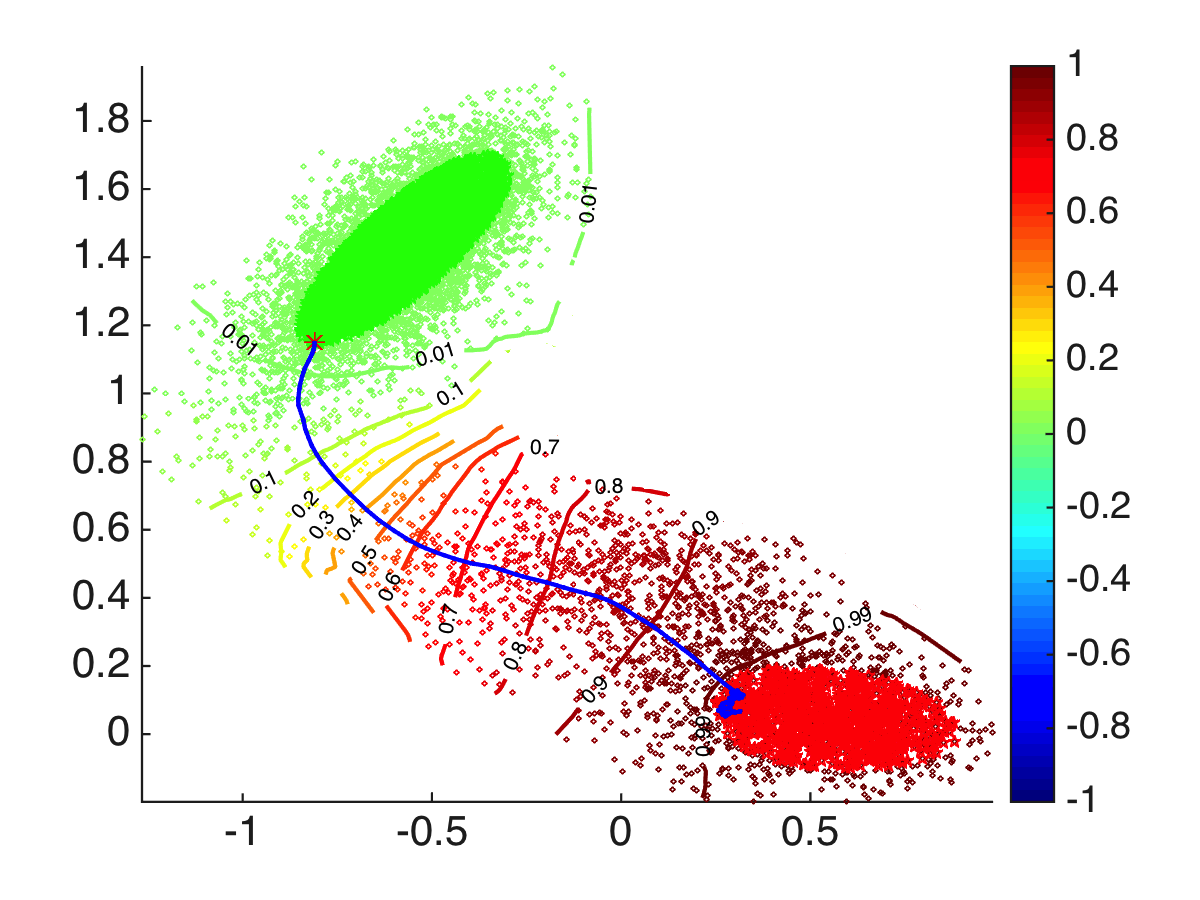
To clearly indicate our method of solving (22), we assume that the given point cloud is sampled on a two dimensional manifold embedded in $\mathbb{R}^{3}$. We emphasize that the following idea can be straightforwardly extended to high dimension cases. Suppose a point $\bm{p}_{c}$ (current point on the reactive flow) has already been obtained, we intend to find the next point on the reactive flow. Without loss of generality, suppose $\bm{p}_{1},\bm{p}_{2},\cdots,\bm{p}_{K}\in\mathcal{P}$ are KNN of $\bm{p}_{c}$ in the point cloud $\mathcal{P}$. Using PCA, we can build a local coordinate system $\{\bm{e}_{\bm{p}_{c}}^{1},\bm{e}_{\bm{p}_{c}}^{2},\bm{e}_{\bm{p}_{c}}^{3}\}$ centered at $\bm{p}_{c}$ and the KNN of $\bm{p}_{c}$ has local coordinates $(x_{i},y_{i},z_{i})$. We use moving least squares (MLS) to locally approximate the surface as $\Gamma=(x,y,z(x,y))$ and estimate $k_{B}T\rho(\bm{p}_{c})\ \nabla q(\bm{p}_{c})$ (more details can be found in [16, 17]). We construct the Delaunay triangulation of the projections $\{\hat{\bm{p}}_{c},\hat{\bm{p}}_{1},\hat{\bm{p}}_{2},\cdots,\hat{\bm{p}}_{K}\}$ and find the first ring $\mathcal{R}=\{T_{c}^{1},\cdots,T_{c}^{l}\}$ of $p_{c}$, which is the same as we did in Section 2.2. Suppose that $k_{B}T\rho(\bm{p}_{c})\ \nabla q(\bm{p}_{c})$ has a local coordinate $(v_{1},v_{2},v_{3})$ in $\{\bm{e}_{\bm{p}_{c}}^{1},\bm{e}_{\bm{p}_{c}}^{2},\bm{e}_{\bm{p}_{c}}^{3}\}$, we find the intersection of line segment starting at $\bm{p}_{c}$ with the direction $(-v_{1},-v_{2},0)$ and the first ring. Notice that this computation is done within the tangent space of $\bm{p}_{c}$. Denote the intersection as $\hat{\bm{p}}_{new}=(x_{0},y_{0},0)$, we then project it back to the approximated surface to obtain the next point on the geodesic path $\bm{p}_{new}=(x_{0},y_{0},z(x_{0},y_{0}))$. This process is illustrated in Figure 9. We refer [14] for more detailed discussion about solving the above equation on point clouds. Figure 10 plots the trajectory starting from the red star point $p_{0}$ in state $A$ to finally hit the region in state $B$, which clearly show that the reactive flow jump from state $A$ to state $B$.

As an advantage of the proposed intrinsic method, the solver we designed can handle point clouds sampled from a low-dimensional manifold in a high dimension space. To illustrate the robustness of the proposed method, we next test the our solver for point clouds embedded in a high dimensional ambient space with an artificial Gaussian noise. In other words, we first simulate 2D point clouds as we conducted in the previous numerical experiments. After that, we embed the point cloud to $\mathbb{R}^{10}$ by setting the last eight coordinates to be zero. In addition, we also perturb this point cloud in $\mathbb{R}^{10}$ by adding Gaussian noise with variance $\sigma=\gamma d_{max}$. Here we choose $d$ to be the maximal number of the 50th smallest distance to each point. Namely, $d_{max}=\max_{i}\{d_{i}~|~d_{i}=\mbox{the 50-th smallest distance to }\bm{p}_{i}\}$. In our experiments, we solve the Fokker-Planck equation based on the point cloud perturbed by Gaussian noise with different level $\gamma=10\%,20\%,50\%,100\%$, and also compute the reactive trajectory from the starting point. For better visualization, figure 11 shows 2D projection of the Gaussian noise perturbed point clouds color-coded with the resulting commitor function $q$. In addition, reactive trajectories are also plotted for different noise level with the same starting point. This figure clearly demonstrates the robustness of the proposed method.

References

- [1] M. Belkin, J. Sun, and Y. Wang, Constructing Laplace operator from point clouds in , in Proceedings of the Twentieth Annual ACM-SIAM Symposium on Discrete Algorithms, Philadelphia, PA, USA, 2009, pp. 1031–1040, http://dl.acm.org/citation.cfm?id=1496770.1496882.
- [2] P. G. Bolhuis, D. Chandler, C. Dellago, and P. L. Geissler, Transition path sampling: throwing ropes over rough mountain passes, in the dark, Annu. Rev. Phys. Chem., 53 (2002), pp. 291–318.
- [3] M. Cameron and E. Vanden-Eijnden, Flows in complex networks: Theory, algorithms, and application to Lennard-Jones cluster rearrangement, J. Stat. Phys., 156 (2014), pp. 427–454.
- [4] R. Coifman, I. Kevrekidis, S. Lafon, M. Maggioni, and B. Nadler, Diffusion maps, reduction coordinates, and low dimensional representation of stochastic systems, Multiscale Model. Simul., 7 (2008), pp. 842–864.
- [5] R. R. Coifman and S. Lafon, Diffusion maps, Appl. Comput. Harmon. Anal., 21 (2006), pp. 5–30.
- [6] C. Dellago, P. G. Bolhuis, and P. L. Geissler, Transition path sampling, Adv. Chem. Phys., 123 (2002).
- [7] G. Dziuk, Finite elements for the beltrami operator on arbitrary surfaces, in Partial differential equations and calculus of variations, Lecture Notes in Math., Springer, Berlin, 1988, pp. 142–155.
- [8] W. E, W. Ren, and E. Vanden-Eijnden, Finite temparture string method for the study of rare events, J. Phys. Chem. B, 109 (2005), pp. 6688–6693.
- [9] W. E and E. Vanden-Eijnden, Toward a theory of transition paths, J. Stat. Phys., 123 (2006), pp. 503–523.
- [10] W. E and E. Vanden-Eijnden, Transition path theory and path-finding algorithms for the study of rare events, Ann. Rev. Phys. Chem., 61 (2010), pp. 391–420.
- [11] G. Hummer, From transition paths to transition states and rate coefficients, J. Chem. Phys., 120 (2004), pp. 516–523.
- [12] I. Jolliffe, Principal component analysis, Wiley Online Library, 2002.
- [13] S. Kirmizialtin and R. Elber, Revisiting and computing reaction coordinates with directional milestoning, J. Phys. Chem. A, 115 (2011), pp. 6137–6148.
- [14] R. Lai, J. Liang, and H.-K. Zhao, A local mesh method for solving PDEs on point clouds, Inverse Probl. Imaging, 7 (2013), pp. 737–755.
- [15] W. Lechner, J. Rogal, J. Juraszek, B. Ensing, and P. G. Bolhuis, Nonlinear reaction coordinate analysis in the reweighted path ensemble, J. Chem. Phys., 133 (2010), p. 174110.
- [16] J. Liang, R. Lai, T. Wong, and H. Zhao, Geometric understanding of point clouds using Laplace-Beltrami operator, Computer Vision and Pattern Recognition (CVPR), (2012), pp. 214–221.
- [17] J. Liang and H. Zhao, Solving partial differential equations on point clouds, SIAM Journal on Scientific Computing, 35 (2013), pp. A1461–A1486.
- [18] A. V. Little, Y.-M. Jung, and M. Maggioni, Multiscale estimation of intrinsic dimensionality of data sets., in AAAI fall symposium: manifold learning and its applications, vol. 9, 2009, p. 04.
- [19] J. Lu and J. Nolen, Reactive trajectories and the transition path process, Probab. Theory Related Fields, 161 (2015), pp. 195–244.
- [20] A. Ma and A. R. Dinner, Automatic method for identifying reaction coordinates in complex systems, J. Phys. Chem. B, 109 (2005), pp. 6769–6779.
- [21] P. Majek and R. Elber, Milestoning without a reaction coordinate, J. Chem. Theory Comput., 6 (2010), pp. 1805–1817.
- [22] R. Metzler, G. Oshanin, and S. Redner, First-passage phenomena and their applications, World Scientific, 2014.
- [23] P. Metzner, C. Schütte, and E. Vanden-Eijnden, Illustration of transition path theory on a collection of simple examples, J. Chem. Phys., (2006), p. 084110.
- [24] P. Metzner, C. Schütte, and E. Vanden-Eijnden, Transition path theory for Markov jump processes, Multiscale Model. Sim., 7 (2009), pp. 1192–1219.
- [25] B. Nadler, S. Lafon, R. R. Coifman, and I. G. Kevrekidis, Diffusion maps, spectral clustering and reaction coordinates of dynamical systems, Appl. Comput. Harmon. Anal., 21 (2006), pp. 113–127.
- [26] B. Peters, Reaction coordinates and mechanicstic hypothesis tests, Ann. Rev. Phys. Chem., 67 (2016), pp. 669–690.
- [27] B. Peters and B. L. Trout, Obtaining reaction coordinates by likelihood maximization, J. Chem. Phys., 125 (2006), p. 054108.
- [28] M. A. Rohrdanz, W. Zheng, M. Maggioni, and C. Clementi, Determination of reaction coordinates via locally scaled diffusion map, J. Chem. Phys., 134 (2011), p. 124116.
- [29] E. Vanden-Eijnden and M. Venturoli, Revisiting the finite temperature string method for the calculation of reaction tubes and free energies, J. Chem. Phys., 130 (2009), p. 194103.
- [30] W. Zheng, M. A. Rohrdanz, M. Maggioni, and C. Clementi, Polymer reversal rate calculated via locally scaled diffusion map, J. Chem. Phys., 134 (2011), p. 144108.