跳到论文正文
W Papers独立论文阅读器 arXiv:1703.08995 论文正文 计算阅读时间 · 0%
引用这篇论文根据当前论文元数据生成,正式投稿前建议核对。


License: arXiv.org perpetual non-exclusive license
arXiv:1703.08995v2 [stat.ME] 18 Apr 2018

The Limit Imbalanced Logistic Regression by Binary Predictors and its fast Lasso computation

Vincent Runge Note: E-mail: runge.vincent@gmail.com Affiliation: LaMME - Laboratoire de Mathématiques et Modélisation d’Evry.
UEVE - Université d’Evry-Val-d’Essonne.
Abstract

In this work, we introduce a modified (rescaled) likelihood for imbalanced logistic regression. This new approach makes easier the use of exponential priors and the computation of lasso regularization path. Precisely, we study a limiting behavior for which class imbalance is artificially increased by replication of the majority class observations. If some strong overlap conditions are satisfied, the maximum likelihood estimate converges towards a finite value close to the initial one (intercept excluded) as shown by simulations with binary predictors. This solution corresponds to the extremum of a strictly concave function that we refer to as ”rescaled” likelihood. In this context, the use of exponential priors has a clear interpretation as a shift on the predictor means for the minority class. Thanks to the simple binary structure, some random designs give analytic path estimators for the lasso regularization problem. An effective approximate path algorithm by piecewise logarithmic functions based on matrix inversions is also presented. This work was motivated by its potential application to spontaneous reports databases in a pharmacovigilance context.

Keywords: path estimator, pharamacovigilance model, piecewise logarithmic approximate path, limit class imbalance, rescaled likelihood, spontaneous reports database, square exact solution.

MS classification : Primary 62J12, 62F12, 62F15; secondary 34E05, 49M29, 62P10.

1 Introduction

If the response y=1y=1 is very rare compared with the response y=0y=0, we are in presence of a rare event configuration also called class imbalance. This problem recently got computer scientists’ attention: they aimed at reducing computational costs by bypassing the class imbalance with resampling methods [12] [21] [6]. With these methods, the variance in estimating model parameters increases. Statisticians are aware of this problem and complex procedures such as local case-control sampling were proposed [8] (a method initiated in epidemiology [19]).

In a recent work (2007) by Art B. Owen [22], the opposite approach is considered: the class imbalance is infinitely increased in order to reach the theoretical distribution of the majority class observations. Owen proved that under some overlap conditions the model parameters are finite (apart from the intercept) and built a limit system of equations related to exponential tilting, whose solution is the new estimate. The resulting equations include the distribution of the infinite class expressed through integrals, which are not easy to infer. This may explain that this work was broadly ignored (The author found it when Sections 2 and 3 were already completed).

In our approach, the observations of the majority class are infinitely replicated and the Owen’s limit distribution becomes the observed distribution. This situation is a kind of degenerate case between resampling (we repeat observations) and infinitely class imbalance (the observed distribution is chosen as the theoretical one). Unlike Owen’s result, our limit normal equations can be interpretated as the first order conditions of a new likelihood.

The idea of this work comes from the analysis of highly imbalanced binary spontaneous reports databases. Such databases are gathered by many countries and institutions (FDA, MHRA, WHO,…). Imbalanced logistic regression with binary predictors gives maximum likelihood estimate (MLE) very close to its limit imbalanced counterpart. This result makes possible the study of lasso-type regularization problem and the development of effective algorithms to provide model selection.

So far, only disproportionality methods are routinely used [18] for spontaneous report databases: predictors are analysed one by one, leading to a great number of false positive signals [13]. Mathematical tools adjusted to binary data for regression are surprisingly barely developed by scientists (only boolean matrices have been studied by some authors [16]). This results in an inflation of empiric methods using lasso regularization in recent years (from [3] to [1]). This is a worrying trend because recommendations made by these experts shift towards more complicated experimental methods and time-consuming algorithms, not towards a deeper mathematical understanding. This work is motivated by the need to better analyse this kind of applied problem.

The paper contains three main sections in which we present the following results:

  • •

    In Section 2, we investigate the properties of the logistic normal equations with binary predictors. Simple existence and uniqueness conditions of Silvapulle’s type are found and some exact solutions presented. An invariance property in presence of intercept links this particular solution (called ”square solution”) to the limit imbalanced problem. We then acquaint ourselves with the issue of variance inflation of the imbalanced problem by computing the Fisher information.

  • •

    In Section 3, we derive Owen-type equations with a first order term evaluating the convergence rate. For the limit system of equations, the existence and uniqueness of the solution is proved with a new method leading to the minimization of a Kullback-Leibler divergence under linear constraints. A rescaling procedure on the initial likelihood and the previously found divergence justify the introduction of a rescaled likelihood corresponding to our limit imbalanced logistic regression problem. In a Bayesian framework, the Jeffreys penalty does not significantly decrease the variance of the estimator but other more appropriate priors, such that exponential ones, could help to reduce it (chosen according to the situation). The closeness in simulation between limit estimates and classical estimates compels us to go one step further with the study of regularization paths, in particular if the model is known to be sparse.

  • •

    In Section 4, we look at a lasso regularization problem for the rescaled likelihood, which has a clear interpretation as a shift on the predictor means for the class of interest. We succeed in finding some path estimators in a few particular cases (independence and orthogonal design). In presence of correlation, we present an effective path following algorithm by piecewise logarithmic functions giving precise estimates. We conclude by explaining the need of an analysis of the correlation structure between predictors. This leads to simple algorithmic procedures with small computational costs for which many different prior penalties could be easily tested. Two examples are given using the French spontaneous reports database.

The expressions ”infinitely imbalance” and ”limit imbalance” are considered as synonymous, although we recommend the use of the second one in our context due to the simple unique limit we impose and an analogy with hydrodynamic limits (in fluid dynamics) while the first expression is related to the underlying distribution introduced by Owen.

We conclude this article by discussing the many opportunities that arise with the introduction of a rescaled likelihood in a Bayesian context and of the path following algorithm by logarithmic functions.

2 The logistic regression by binary predictors

2.1 Logistic normal equations

The binary logistic regression (BLR) problem consists in the determination of coefficients β^\hat{\beta} maximizing a smooth and concave likelihood function given by the relation

L⁡(β|I0,I1,n0,n1)=∏i=1q1(e(I1​β)i1+e(I1​β)i)ni1​∏i=1q0(1+e(I0​β)i)−ni0,L(\beta|I_{0},I_{1},n^{0},n^{1})=\prod_{i=1}^{q_{1}}\left(\frac{e^{(I_{1}\beta)_{i}}}{1+e^{(I_{1}\beta)_{i}}}\right)^{n_{i}^{1}}\prod_{i=1}^{q_{0}}\left(1+e^{(I_{0}\beta)_{i}}\right)^{-n_{i}^{0}}\,,

where β=(βi)∈ℝp+1\beta=(\beta_{i})\in\mathbb{R}^{p+1} is indexed from zero with β0\beta_{0} corresponding to the intercept. Binary design matrices I1∈ℳq1×(p+1)​(𝔹)I_{1}\in\mathcal{M}_{q_{1}\times(p+1)}(\mathbb{B}) and I0∈ℳq0×(p+1)​(𝔹)I_{0}\in\mathcal{M}_{q_{0}\times(p+1)}(\mathbb{B}) with 𝔹={0,1}\mathbb{B}=\{0,1\} are of full rank: they aggregate the pp binary predictors. Vectors of weights n0=(n10,…,nq00)T∈(ℕ∗)q0n^{0}=(n_{1}^{0},...,n_{q_{0}}^{0})^{T}\in(\mathbb{N}^{*})^{q_{0}} and n1=(n11,…,nq11)T∈(ℕ∗)q1n^{1}=(n_{1}^{1},...,n_{q_{1}}^{1})^{T}\in(\mathbb{N}^{*})^{q_{1}} save repetitions for distinct observations in response classes 00 and 11 separately. The binary structure favours repetitions in the sequence of observations, which justifies these notations. Moreover (I0​β)i(I_{0}\beta)_{i} is the i-th component of vector I0​β∈ℝq0I_{0}\beta\in\mathbb{R}^{q_{0}} (the same for (I1​β)i(I_{1}\beta)_{i}).

We introduce other notations thereafter used within this article. The modulus of a vector denotes its l1l^{1} norm, while the overline sign on lower cases stands for l1l^{1} normalization. For example |n1|=∑i=1q1ni1|n^{1}|=\sum_{i=1}^{q_{1}}n_{i}^{1} and n¯i1=ni1/|n1|\overline{n}^{1}_{i}=n^{1}_{i}/|n^{1}| gives the vector n¯1\overline{n}^{1}. AiA_{i} is the i-th row of the matrix AA and its roman upper case equivalent 𝙰\mathtt{A} is the matrix AA in which the first column filled by ones (associated to the intercept) was removed. We also need N1=𝙸1T​n1∈ℝpN^{1}=\mathtt{I}_{1}^{T}n^{1}\in\mathbb{R}^{p} with TT standing for the matrix transpose operator. An important feature in our study is the predictor means vector N¯1\overline{N}^{1} for class 11 obtained by the relation 𝙸1T​n¯1=N¯1\mathtt{I}^{T}_{1}\overline{n}^{1}=\overline{N}^{1}. For vectors of same size u,v∈ℝqu,\,v\in\mathbb{R}^{q}, u​vuv (resp. uv\frac{u}{v}) is the vector with components uk​vku_{k}v_{k} (resp. ukvk\frac{u_{k}}{v_{k}}), k∈{1,…,q}k\in\{1,...,q\}. β~\tilde{\beta} is the vector β\beta without the intercept coefficient β0\beta_{0}. From Subsection 3.2, the notations II and 𝙸\mathtt{I} for matrices I0I_{0} and 𝙸0\mathtt{I}_{0} respectively are often used (as well as qq for integer q0q_{0}).

For ease of calculation, we consider the opposite of the log-likelihood. If I1=I0=ℐI_{1}=I_{0}=\mathcal{I}, we have q1=q0=qq_{1}=q_{0}=q and we can introduce vectors n=n1+n0n=n^{1}+n^{0} and Δ​n=n1−n0\Delta n=n^{1}-n^{0}. In this latter case, we write

l⁡(β)=−log⁡(L⁡(β))=|n|​log​2+∑i=1q(−Δ​ni​(12​(ℐ​β)i)+ni​log​cosh⁡(12​(ℐ​β)i)),l(\beta)=-\log(L(\beta))=|n|\log 2+\sum_{i=1}^{q}\left(-\Delta n_{i}(\frac{1}{2}(\mathcal{I}\beta)_{i})+n_{i}\log\cosh(\frac{1}{2}(\mathcal{I}\beta)_{i})\right)\,,

and first order conditions are computed, differentiating ll with respect to each βj\beta_{j} coefficient. We obtain

0=∂l⁡(β)∂βj=∑i=1q(−Δ​ni​(12​ℐi​j)+12​ni​ℐi​j​tanh⁡(12​(ℐ​β)i)),j∈{0,…,p},0=\frac{\partial l(\beta)}{\partial\beta_{j}}=\sum_{i=1}^{q}\left(-\Delta n_{i}(\frac{1}{2}\mathcal{I}_{ij})+\frac{1}{2}n_{i}\mathcal{I}_{ij}\tanh(\frac{1}{2}(\mathcal{I}\beta)_{i})\right)\,,\quad j\in\{0,...,p\}\,,

or in matrix form

ℐT​Δ​n=ℐT​(n​tanh⁡(12​ℐ​β)).\mathcal{I}^{T}\Delta n=\mathcal{I}^{T}\left(n\tanh(\frac{1}{2}\mathcal{I}\beta)\right)\,. (2.1)

In a general framework with non-identical matrices I0I_{0} and I1I_{1}, we likewise derive

I1T​n1−I0T​n0=I1T​(n1​tanh⁡(12​I1​β))+I0T​(n0​tanh⁡(12​I0​β)).I_{1}^{T}n^{1}-I_{0}^{T}n^{0}=I_{1}^{T}\left(n^{1}\tanh(\frac{1}{2}I_{1}\beta)\right)+I_{0}^{T}\left(n^{0}\tanh(\frac{1}{2}I_{0}\beta)\right)\,. (2.2)

This system of equations (2.2) gathers the so-called logistic normal equations and will be widely used within this article.

Remark 2.1.

These equations are usually presented with a logistic function but we chose another expression to highlight the link with existence and uniqueness conditions.

2.2 Existence and uniqueness

Necessary and sufficient conditions to ensure existence and uniqueness of the MLE are well-known, they were established by Silvapulle in 1981 [27]. They consist in satisfying an overlap condition C1∩C0≠∅C_{1}\cap C_{0}\neq\emptyset between the cones

C1={I1T​u1|u1∈(ℝ+∗)q1}​and​C0={I0T​u0|u0∈(ℝ+∗)q0}.C_{1}=\left\{I_{1}^{T}u_{1}\,|\,u_{1}\in(\mathbb{R}^{*}_{+})^{q_{1}}\right\}\,\,\hbox{and}\,\,C_{0}=\left\{I_{0}^{T}u_{0}\,|\,u_{0}\in(\mathbb{R}^{*}_{+})^{q_{0}}\right\}\,.

For the BLR problem, a more convenient description is possible:

Theorem 2.1.

The BLR problem admits a unique solution if and only if there exist n+∈(ℕ∗)q1n^{+}\in(\mathbb{N}^{*})^{q_{1}} and n∗∈(ℕ∗)q0n^{*}\in(\mathbb{N}^{*})^{q_{0}}, such that I1T​n+=I0T​n∗I_{1}^{T}n^{+}=I_{0}^{T}n^{*}.

Looking at equations (2.2), this theorem means that a MLE exists and is unique if one can find a couple (n+,n∗)(n^{+},n^{*}) of observations of the rows in I1I_{1} and in I0I_{0} such that |n+|=|n∗||n^{+}|=|n^{*}| vanishing all the regression coefficients (intercept included). An easy necessary condition to check is that at least one 00 and one 11 are present in each column of I0I_{0} and I1I_{1} (at the exception of the first column of ones corresponding to intercept).

Proof.

If I1T​n+=I0T​n∗I_{1}^{T}n^{+}=I_{0}^{T}n^{*}, the Silvapulle’s condition is immediately verified. Reciprocally, C1∩C0C_{1}\cap C_{0} is an open subset of ℝp+1\mathbb{R}^{p+1} with positive measure because I0I_{0} and I1I_{1} are full rank matrices. By a density argument, there exist q∈(ℚ∩]0,1[)p+1q\in(\mathbb{Q}\cap]0,1[)^{p+1}, λ∈(ℝ+∗)q0\lambda\in(\mathbb{R}^{*}_{+})^{q_{0}} and μ∈(ℝ+∗)q1\mu\in(\mathbb{R}^{*}_{+})^{q_{1}} satisfying I0T​λ=I1T​μ=qI^{T}_{0}\lambda=I^{T}_{1}\mu=q. We reorder the rows in I0I_{0} and I1I_{1} such that the first p+1p+1 rows are linearly independent. Let H0H_{0} in ℳq0×(q0−p−1)​(ℝ)\mathcal{M}_{q_{0}\times(q_{0}-p-1)}(\mathbb{R}) and H1H_{1} in ℳq1×(q1−p−1)​(ℝ)\mathcal{M}_{q_{1}\times{(q_{1}-p-1)}}(\mathbb{R}) be orthogonal matrices to I0I_{0} and I1I_{1} respectively. Because of the reorganization of the rows in IiI_{i} (i∈{0,1}i\in\{0,1\}) we can choose a HiH_{i} where its last qi−p−1q_{i}-p-1 rows form an identity matrix 𝕀qi−p−1\mathbb{I}_{q_{i}-p-1}. For all α0∈ℝq0−p−1\alpha_{0}\in\mathbb{R}^{q_{0}-p-1} and α1∈ℝq1−p−1\alpha_{1}\in\mathbb{R}^{q_{1}-p-1} we have the relation I0T​(λ+H0​α0)=I1T​(μ+H1​α1)=qI^{T}_{0}(\lambda+H_{0}\alpha_{0})=I^{T}_{1}(\mu+H_{1}\alpha_{1})=q. Again with a density argument, we find α0\alpha_{0} such that λi+(α0)i∈ℚ+∗\lambda_{i}+(\alpha_{0})_{i}\in\mathbb{Q}^{*}_{+} for all i∈{p+2,…,q0}i\in\{p+2,...,q_{0}\} and satisfying the constraint λ+H0​α0∈(ℝ+∗)q0\lambda+H_{0}\alpha_{0}\in(\mathbb{R}_{+}^{*})^{q_{0}}. For a matrix A∈ℳn×m​(ℝ)A\in\mathcal{M}_{n\times m}(\mathbb{R}), a vector v∈ℝmv\in\mathbb{R}^{m} and J⊂{1,…,m}J\subset\{1,...,m\}, let [A​v]J[Av]_{J} denote the vector AJ​vJA_{J}v_{J}, where AJA_{J} (resp. vJv_{J}) corresponds to the submatrix of AA (resp. subvector of vv) obtained by removing from AA (resp. from vv) the columns (resp. rows) that do not correspond to the indices in JJ. With this notation, we have [I0T​(λ+H0​α0)]{1,…,p+1}=q−[I0T​(λ+H0​α0)]{p+2,…,q0}∈ℚp+1[I^{T}_{0}(\lambda+H_{0}\alpha_{0})]_{\{1,...,p+1\}}=q-[I^{T}_{0}(\lambda+H_{0}\alpha_{0})]_{\{p+2,...,q_{0}\}}\in\mathbb{Q}^{p+1}. The binary matrix (I0T){1,…,p+1}(I^{T}_{0})_{\{1,...,p+1\}} is then nonsingular and using its inverse in ℳ(p+1)×(p+1)​(ℚ)\mathcal{M}_{(p+1)\times(p+1)}(\mathbb{Q}) we obtain (λ+H0​α0){1,…,p+1}∈(ℚ+∗)p+1(\lambda+H_{0}\alpha_{0})_{\{1,...,p+1\}}\in(\mathbb{Q}_{+}^{*})^{p+1}. Finally α0∗=λ+H0​α0∈(ℚ+∗)q0\alpha_{0}^{*}=\lambda+H_{0}\alpha_{0}\in(\mathbb{Q}_{+}^{*})^{q_{0}}. The same arguments lead to a set of coefficients α1∗=μ+H1​α1∈(ℚ+∗)q1\alpha_{1}^{*}=\mu+H_{1}\alpha_{1}\in(\mathbb{Q}_{+}^{*})^{q_{1}}. Multiplying the vector (α0∗,α1∗)(\alpha_{0}^{*},\alpha_{1}^{*}) by the ppcm of all its denominators proves the result.∎

2.3 The square case

The situation with identical square design matrices I0I_{0} and I1I_{1} is worthwhile in itself because it leads to explicit analytic formulae for the MLE and their variance (in the asymptotic case). In particular, we focus on the introduction of imbalance between n1n^{1} and n0n^{0} to emphasize the simple solution for MLE and the problem of variance inflation.

Theorem 2.2.

If I0=I1=II_{0}=I_{1}=\mathrm{I} is a square matrix, we have the following closed form for the maximum likelihood estimator:

β^=I−1​log⁡(n1n0).\hat{\beta}=\mathrm{I}^{-1}\log\left(\frac{n^{1}}{n^{0}}\right)\,. (2.3)
Proof.

the matrix I\mathrm{I} verifies the condition q=p+1q=p+1 and is nonsingular with I−1\mathrm{I}^{-1} its inverse (because I\mathrm{I} is of full rank). The vector TT is defined as T=tanh⁡(12​I​β)∈ℝp+1T=\tanh\left(\frac{1}{2}\mathrm{I}\beta\right)\in\mathbb{R}^{p+1} i.e. I​β=log⁡(1+T1−T)\mathrm{I}\beta=\log\left(\frac{1+T}{1-T}\right). Multiplying (2.1) by (I−1)T=(IT)−1(\mathrm{I}^{-1})^{T}=(\mathrm{I}^{T})^{-1}, we get T=Δ​nnT=\frac{\Delta n}{n}. Hence, β=I−1​log⁡(n+Δ​nn−Δ​n)\beta=\mathrm{I}^{-1}\log\left(\frac{n+\Delta n}{n-\Delta n}\right), which achieves the proof. ∎

Remark 2.2.

If one of the components in the vectors of weights n1n^{1} or n0n^{0} vanishes, some of the regression coefficients become infinite (but not necessarily all of them).

To our knowledge, this is the first general closed form found in the resolution of a logisitic regression. There exist partial results for a unique categorical predictor exposed by Lipovetsky in 2014 [17]. An explanation for the lack of such a simple result stands in the poorly studied finite observation structure made possible through binary predictors with repetitions. In Appendix A, some particular solutions to equations (2.3) are presented.

2.3.1 Invariance if intercept

We establish an invariance property making a link with the imbalanced problem.

Proposition 2.1.

In the square case with intercept, multiplying all the components of n1n^{1} or n0n^{0} by a same integer does not change the value of the MLE apart from the intercept.

Proof.

The inverse of a matrix with an intercept term verifies the relation

I−1​(11)=(100),\mathrm{I}^{-1}\begin{pmatrix}1\\ \vdots\\ 1\\ \end{pmatrix}=\begin{pmatrix}1\\ 0\\ \vdots\\ 0\\ \end{pmatrix}\,,

which means that we can rewrite equations (2.3) as

β^i=log⁡(∏j=0p(nj1nj0)ai​j),i∈{0,…,p},ai​j=(I−1)i​j​and​∑j=0pai​j=δ0​i.\hat{\beta}_{i}=\log\left(\prod_{j=0}^{p}\left(\frac{n^{1}_{j}}{n^{0}_{j}}\right)^{a_{ij}}\right)\,,\,i\in\{0,...,p\}\,,\,\,a_{ij}=(\mathrm{I}^{-1})_{ij}\,\,\hbox{and}\,\,\sum_{j=0}^{p}a_{ij}=\delta_{0i}\,.

Substituting nj0n_{j}^{0} by s×nj0s\times n_{j}^{0} (or nj1n_{j}^{1} by s×nj1s\times n_{j}^{1}) with s∈ℕ∗s\in\mathbb{N}^{*} gives the same result for all βi,i∈{1,…,p}\beta_{i}\,,\,i\in\{1,...,p\}. ∎

2.3.2 Asymptotic variance

To conclude this section, we study the asymptotic behavior of the estimator for large |n1||n^{1}| and |n0||n^{0}|. Since the MLE (intercept excluded) remains the same with or without a class imbalance (see the invariance property), we have a glimpse of a general property in class imbalance.

Proposition 2.2.

In the square case BLR problem, the variance of the maximum likelihood estimator is approximately given by relations

V⁡(β^i)≈∑j=0pai​j2​(1nj1+1nj0),i∈{0,…,p},ai​j=(I−1)i​j.V(\hat{\beta}_{i})\approx\sum_{j=0}^{p}a_{ij}^{2}\left(\frac{1}{n_{j}^{1}}+\frac{1}{n_{j}^{0}}\right)\,,\quad i\in\{0,...,p\}\,,\quad a_{ij}=(\mathrm{I}^{-1})_{ij}\,.
Proof.

We compute the observed Fisher information ℐ⁡(β^)=IT​D​I\mathcal{I}(\hat{\beta})=\mathrm{I}^{T}D\mathrm{I} with DD a diagonal matrix with elements ni​p^i​(1−p^i)n_{i}\hat{p}_{i}(1-\hat{p}_{i}) and p^i=1/(1+e−(I​β^)i)\hat{p}_{i}=1/(1+e^{-(I\hat{\beta})_{i}}). Its inverse gives the desired result, knowing that ni​p^i=ni1n_{i}\hat{p}_{i}=n_{i}^{1} and ni​(1−p^i)=ni0n_{i}(1-\hat{p}_{i})=n_{i}^{0}. ∎

Remark 2.3.

Another method uses the closed form (2.3) to perform variance and bias estimations by Taylor expansions with the multinomial random vector (n1,n0)(n^{1},n^{0}). We obtain V⁡(β^i)≈∑j=0pai​j2​(1nj1+1nj0−2|n|)V(\hat{\beta}_{i})\approx\sum_{j=0}^{p}a_{ij}^{2}(\frac{1}{n_{j}^{1}}+\frac{1}{n_{j}^{0}}-\frac{2}{|n|}) and B​i​a​s​(β^i)≈∑j=0pai​j2​(1nj0−1nj1),i∈{0,…,p}Bias(\hat{\beta}_{i})\approx\sum_{j=0}^{p}\frac{a_{ij}}{2}(\frac{1}{n_{j}^{0}}-\frac{1}{n_{j}^{1}})\,,i\in\{0,...,p\}\,. However, simulations give inaccurate results and only the Fisher information method should be retained.

We investigate the variation of the variance with respect to the sample size |n||n| and the value of the intercept β0\beta_{0} for a simple fixed model (β1,…,β5)=(−0.5,−0.25,0,0.25,0.5)(\beta_{1},...,\beta_{5})=(-0.5,-0.25,0,0.25,0.5). With these two parameters given, we simulate 10410^{4} data sets with a different random binary square matrix I\mathrm{I} and different random vectors n1n^{1} and n0n^{0} for each of them (but |n1|+|n0||n^{1}|+|n^{0}| is fixed). In table 1, we compare the estimated standard deviation (sd.) with the Fisher standard deviation given in Proposition 2.2 (F.sd.) accompanied by an estimation of the bias (bias) for coefficient β4=0.25\beta_{4}=0.25.

β0\beta_{0} -7 -6 -5 -4 -3 -2 -1 0
|n||n| |n0|/|n1||n_{0}|/|n_{1}| 1052 385 142 52 19 7.1 2.7 1.0
sd. . . . . 0.768 0.467 0.333 0.286
10310^{3} F.sd. . . . . 0.762 0.464 0.334 0.293
bias . . . . 0.019 0.0037 0.0065 -0.0021
sd. . . 0.633 0.369 0.224 0.145 0.105 0.0931
10410^{4} F.sd. . . 0.618 0.361 0.221 0.145 0.104 0.0918
bias . . 0.019 9.4e-3 -2.4e-4 1.e-3 -3.0e-4 -2.9e-4
sd. 0.528 0.303 0.187 0.110 0.0690 0.0450 0.0328 0.0300
10510^{5} F.sd. 0.512 0.301 0.183 0.111 0.0685 0.0451 0.0327 0.0291
bias 0.020 5.4e-4 3.4e-3 -3.2e-5 -5.6e-5 4.5e-4 -2.8e-5 1.9e-4
Table 1: Variance analysis in the square case with intercept for coefficient β4=0.25\beta_{4}=0.25. We used the following quantities : (sd.)2=10−4∑i=1104(0.25−(β^4)i)2(sd.)^{2}=10^{-4}\sum_{i=1}^{10^{4}}(0.25-(\hat{\beta}_{4})_{i})^{2}, (F.sd.)2=10−4∑i=1104V(β^4)i(F.sd.)^{2}=10^{-4}\sum_{i=1}^{10^{4}}V(\hat{\beta}_{4})_{i} and b​i​a​s=10−4​∑i=1104(0.25−(β^4)i)bias=10^{-4}\sum_{i=1}^{10^{4}}(0.25-(\hat{\beta}_{4})_{i}).

These simulations highlight the accuracy of the ”Fisher variance” in all configurations, which is very close to the estimated one. Bias is negligible compared with variance. For a constant number of observations |n||n|, the variance increases when the disbalance between classes strengthens. This variance inflation is a key issue in class imbalance, we further explain how one can easily add a prior information to a rescaled likelihood to deal with this problem (see Subsection 3.4).

3 Limit imbalanced study

3.1 Owen-type equations

The limit case consists in infinitely replicating the majority class observations as if the theoretical distribution of this class was the observed one. This is a degenerate case of the Owen’s study, that is why we know that the intercept coefficient tends to minus infinity whereas other regression coefficients are finite if a stronger overlap condition is satisfied [22]. For the limit equations, an information reduction for the majority class occurs: only the means of the predictors matter, the correlation structure in this class of interest ”disappears”.

The following proposition presents the logistic normal equations (2.2) in a new form with a remainder term arising in case of class imbalance.

Proposition 3.1.

For an imbalanced binary logisitic regression with a class size for response y=0y=0 ’ss’ times greater than the one for response y=1y=1, we obtained the system of equations

𝕟𝟙𝟘n10=N¯1+1s​(n20(n10)2​(𝕟𝟚𝟘n20−N¯1)−n11n10​(𝕟𝟙𝟙n11−N¯1))+o⁡(1s),\frac{\mathbb{n_{1}^{0}}}{n_{1}^{0}}=\overline{N}^{1}+\frac{1}{s}\left(\frac{n_{2}^{0}}{(n_{1}^{0})^{2}}\left(\frac{\mathbb{n_{2}^{0}}}{n_{2}^{0}}-\overline{N}^{1}\right)-\frac{n_{1}^{1}}{n_{1}^{0}}\left(\frac{\mathbb{n_{1}^{1}}}{n_{1}^{1}}-\overline{N}^{1}\right)\right)+o(\frac{1}{s})\,,

with s=|n0||n1|≫1s=\frac{|n^{0}|}{|n^{1}|}\gg 1. We used notations:

n10=∑i=1q0n¯i0​e(𝙸0​β~)i,n11=∑i=1q1n¯i1​e(𝙸1​β~)i,n20=∑i=1q0n¯i0​e2​(𝙸0​β~)i,n21=∑i=1q1n¯i1​e2​(𝙸1​β~)i,n_{1}^{0}=\sum_{i=1}^{q_{0}}\overline{n}^{0}_{i}e^{(\mathtt{I}_{0}\tilde{\beta})_{i}}\,,\,\,n_{1}^{1}=\sum_{i=1}^{q_{1}}\overline{n}^{1}_{i}e^{(\mathtt{I}_{1}\tilde{\beta})_{i}}\,,\,\,n_{2}^{0}=\sum_{i=1}^{q_{0}}\overline{n}^{0}_{i}e^{2(\mathtt{I}_{0}\tilde{\beta})_{i}}\,,\,\,n_{2}^{1}=\sum_{i=1}^{q_{1}}\overline{n}^{1}_{i}e^{2(\mathtt{I}_{1}\tilde{\beta})_{i}}\,,

and for vectors in ℝp\mathbb{R}^{p}:

𝕟𝟙𝟘=𝙸0T​(n¯0​e𝙸0​β~),𝕟𝟙𝟙=𝙸1T​(n¯1​e𝙸1​β~),𝕟𝟚𝟘=𝙸0T​(n¯0​e2​𝙸0​β~),𝕟𝟚𝟙=𝙸1T​(n¯1​e2​𝙸1​β~).\mathbb{n_{1}^{0}}=\mathtt{I}_{0}^{T}(\overline{n}^{0}e^{\mathtt{I}_{0}\tilde{\beta}})\,,\,\,\mathbb{n_{1}^{1}}=\mathtt{I}_{1}^{T}(\overline{n}^{1}e^{\mathtt{I}_{1}\tilde{\beta}})\,,\,\,\mathbb{n_{2}^{0}}=\mathtt{I}_{0}^{T}(\overline{n}^{0}e^{2\mathtt{I}_{0}\tilde{\beta}})\,,\,\,\mathbb{n_{2}^{1}}=\mathtt{I}_{1}^{T}(\overline{n}^{1}e^{2\mathtt{I}_{1}\tilde{\beta}})\,.

The technical proof of this result is exposed in Appendix B.

As shown by simulations (see table 2), the first order and remainder terms are negligible quantities with binary predictors, even if there is no imbalance! This suggests the introduction of the following limit imbalanced equations, obtained with s=+∞s=+\infty in Proposition 3.1.

Theorem 3.1.

For infinitely imbalanced binary logisitic regression verifying a strong overlap condition (see Theorem 3.2), the following system of pp limit imbalanced equations holds11 1 With non-binary design matrices X1X_{1} and X0X_{0} and no vectors of weights, we obtain 𝚇0T​(e𝚇0​β~∑ie(𝚇0​β~)i)=N¯1.\mathtt{X}_{0}^{T}\left(\frac{e^{\mathtt{X}_{0}\tilde{\beta}}}{\sum_{i}e^{(\mathtt{X}_{0}\tilde{\beta})_{i}}}\right)=\overline{N}^{1}\,. These equations also differ from Owen’s [22].

𝙸0T​(n¯0​e𝙸0​β~∑in¯i0​e(𝙸0​β~)i)=N¯1.\mathtt{I}_{0}^{T}\left(\frac{\overline{n}^{0}e^{\mathtt{I}_{0}\tilde{\beta}}}{\sum_{i}\overline{n}^{0}_{i}e^{(\mathtt{I}_{0}\tilde{\beta})_{i}}}\right)=\overline{N}^{1}\,. (3.1)

Notice that the β~\tilde{\beta} coefficients do not depend on the structure in rows of the design matrix associated to response y=1y=1 but only on the means of ones for each predictor: N¯1\overline{N}^{1}.

We give a direct simple proof, avoiding the complicated previous proof of Appendix B.

Proof.

For xx near minus infinity, the hyperbolic tangent has the following first order expansion:

tanh⁡(x2)=−1+2​ex+o⁡(ex).\tanh\left(\frac{x}{2}\right)=-1+2e^{x}+o(e^{x})\,.

From [22] we know that the intercept term tends to minus infinity, then with x=I0​βx=I_{0}\beta or x=I1​βx=I_{1}\beta, we use the previous expansion neglecting the remainder term. Thus, equations (2.2) become

I1T​n1=I1T​(n1​eI1​β)+I0T​(n0​eI0​β),I_{1}^{T}n^{1}=I_{1}^{T}\left(n^{1}e^{I_{1}\beta}\right)+I_{0}^{T}\left(n^{0}e^{I_{0}\beta}\right)\,, (3.2)

and factoring by exp⁡(β0)\exp(\beta_{0}) in the first equation of this system we have

exp⁡(β0)=|n1|∑i=1q1ni1​e(𝙸1​β~)i+∑i=1q0ni0​e(𝙸0​β~)i≈|n1|∑i=1q0ni0​e(𝙸0​β~)i,\exp(\beta_{0})=\frac{|n^{1}|}{\sum_{i=1}^{q_{1}}n_{i}^{1}e^{(\mathtt{I}_{1}\tilde{\beta})_{i}}+\sum_{i=1}^{q_{0}}n_{i}^{0}e^{(\mathtt{I}_{0}\tilde{\beta})_{i}}}\approx\frac{|n^{1}|}{\sum_{i=1}^{q_{0}}n_{i}^{0}e^{(\mathtt{I}_{0}\tilde{\beta})_{i}}}\,, (3.3)

because |n0||n1|→+∞\frac{|n^{0}|}{|n^{1}|}\to+\infty. Looking back at (3.2) without the first equation, we have

𝙸1T​n¯1=𝙸1T​(n1​e𝙸1​β~∑i=1q0ni0​e(𝙸0​β~)i)+𝙸0T​(n0​e𝙸0​β~∑i=1q0ni0​e(𝙸0​β~)i)\mathtt{I}_{1}^{T}\overline{n}^{1}=\mathtt{I}_{1}^{T}\left(\frac{n^{1}e^{\mathtt{I}_{1}\tilde{\beta}}}{\sum_{i=1}^{q_{0}}n_{i}^{0}e^{(\mathtt{I}_{0}\tilde{\beta})_{i}}}\right)+\mathtt{I}_{0}^{T}\left(\frac{n^{0}e^{\mathtt{I}_{0}\tilde{\beta}}}{\sum_{i=1}^{q_{0}}n_{i}^{0}e^{(\mathtt{I}_{0}\tilde{\beta})_{i}}}\right)

but

n1​e𝙸1​β~∑i=1q0ni0​e(𝙸0​β~)i=|n1||n0|​n¯1​e𝙸1​β~∑i=1q0n¯i0​e(𝙸0​β~)i→0\frac{n^{1}e^{\mathtt{I}_{1}\tilde{\beta}}}{\sum_{i=1}^{q_{0}}n_{i}^{0}e^{(\mathtt{I}_{0}\tilde{\beta})_{i}}}=\frac{|n^{1}|}{|n^{0}|}\frac{\overline{n}^{1}e^{\mathtt{I}_{1}\tilde{\beta}}}{\sum_{i=1}^{q_{0}}\overline{n}_{i}^{0}e^{(\mathtt{I}_{0}\tilde{\beta})_{i}}}\to 0

because |n1||n0|→0\frac{|n^{1}|}{|n^{0}|}\to 0 and we obtain the desired result. ∎

In table 2, we present simulation results based on limit imbalanced equations (3.1) compared with classical logistic regression (2.2). The sample procedure is the same as the one used for table 1 except that we fixed sample size at |n|=|n1|+|n0|=104|n|=|n^{1}|+|n^{0}|=10^{4} and vary dimension for the matrix I0I_{0} (we chose q0=10,21,32q_{0}=10,21,32).

β0\beta_{0} -5 -4 -3 -2 -1 0
q0q_{0} |n0|/|n1||n^{0}|/|n^{1}| 141 51 19 7.0 2.6 1.0
sd. 0.3614 0.2154 0.1331 0.08765 0.06384 0.05730
sd. imb. 0.3614 0.2154 0.1331 0.08766 0.06402 0.05757
1010 bias 2.533e-3 7.572e-4 -9.553e-4 1.407e-3 2.797e-4 4.954e-4
bias imb. 2.532e-3 7.527e-4 -9.433e-4 1.439e-3 3.261e-4 5.073e-4
l1l^{1} 4.702e-4 6.849e-4 1.089e-3 1.762e-3 2.869e-3 4.806e-3
sd. 0.2643 0.1583 0.09879 0.06468 0.04839 0.04382
sd. imb. 0.2643 0.1583 0.09879 0.06474 0.04860 0.04451
2121 bias 2.148e-3 1.956e-3 -1.583e-5 7.601e-4 2.461e-4 -6.280e-4
bias imb. 2.130e-3 1.967e-3 -8.450e-6 7.752e-4 3.000e-4 -5.337e-4
l1l^{1} 5.950e-4 8.864e-4 1.399e-3 2.281e-3 3.698e-3 5.952e-3
sd. 0.2438 0.1470 0.09346 0.06112 0.04585 0.04090
sd. imb. 0.2438 0.1471 0.09349 0.06117 0.04628 0.04171
3232 bias 4.385e-3 1.034e-3 8.025e-4 3.584e-4 1.259e-3 -1.905e-4
bias imb. 4.383e-3 1.048e-3 7.894e-4 3.537e-4 1.313e-3 -4.297e-5
l1l^{1} 6.220e-4 9.239e-4 1.472e-3 2.341e-3 3.920e-3 6.306e-03
Table 2: Variance and bias analysis in standard and imbalanced situations for coefficient β4=0.25\beta_{4}=0.25. The l1l^{1} is given by the formula l1=10−4​∑i=1104|(β^4i​m​b)i−(β^4)i|l^{1}=10^{-4}\sum_{i=1}^{10^{4}}|(\hat{\beta}_{4}^{imb})_{i}-(\hat{\beta}_{4})_{i}|.

The two estimates β^4\hat{\beta}_{4} for standard and imbalanced regressions are very close to each other as shown by the mean of the l1l^{1} norm – even if the problem is not imbalanced – so that standard deviation and bias are almost the same. This means that, if interesting properties can be established with the limit equations, this context will be appropriate to highlight new features in classical logistic regression.

The 1/s1/s first order term in Proposition 3.1 should be estimated to understand how good the limit imbalanced approximation is, without having to estimate the standard regression coefficients. Simulations show that this term is very small and we choose not to dwell on this intermediate situation, but it could be a more important result if non-binary design matrices are involved.

3.2 Strong overlap condition and rescaled likelihood

Existence and uniqueness conditions to solve (3.1) are well-known [22], they consist in an overlap condition a little bit stronger than the one given by Silvapulle. In fact, we need the point N¯1\overline{N}^{1} to be surrounded by the rows of 𝙸0\mathtt{I}_{0} (hereafter denoted by the letter 𝙸\mathtt{I}). We give this result in the framework of the binary problem (simpler than Owen’s general case) and establish a new proof leading to a minimum relative entropy problem. From there and using duality, we build the corresponding rescaled likelihood also justified by a rescaling on the initial likelihood.

Theorem 3.2.

There exists a unique finite solution to the limit imbalanced BLR problem if and only if there exists λ∈(ℝ+∗)q\lambda\in(\mathbb{R}_{+}^{*})^{q} such that 𝙸T​λ=N¯1\mathtt{I}^{T}\lambda=\overline{N}^{1} and ∑i=1qλi=1\sum_{i=1}^{q}\lambda_{i}=1. (If present, the null row (such that 𝙸i=(0,…,0)\mathtt{I}_{i}=(0,...,0)) is removed22 2 in order to have non-zero coefficients λ\lambda as for the overlap condition in Theorem 2.1..)

Remark 3.1.

The condition 𝙸T​λ=N¯1\mathtt{I}^{T}\lambda=\overline{N}^{1} means that we have I0T​λ=I1T​n¯1I^{T}_{0}\lambda=I^{T}_{1}\overline{n}^{1} with λ∈(ℝ+∗)q0\lambda\in(\mathbb{R}_{+}^{*})^{q_{0}} and n¯1∈(ℝ+∗)q1\overline{n}^{1}\in(\mathbb{R}_{+}^{*})^{q_{1}} so that C1∩C0≠∅C_{1}\cap C_{0}\neq\emptyset. In other words, the existence and uniqueness of a solution for the limit problem implies existence and uniqueness for its associated BLR problem.

Our proof of this theorem is based on the following three lemmas.

Lemma 3.1.

The log-sum-exp function h:ℝq↦ℝh:\mathbb{R}^{q}\mapsto\mathbb{R}, defined by h⁡(z)=log⁡(∑i=1qezi)h(z)=\log(\sum_{i=1}^{q}e^{z_{i}}) is a convex, continuous, increasing function on ℝq\mathbb{R}^{q}. The function f:ℝp↦ℝf:\mathbb{R}^{p}\mapsto\mathbb{R}, f⁡(β~)=log⁡(∑i=1qn¯i0​e(𝙸​β~)i)f(\tilde{\beta})=\log(\sum_{i=1}^{q}\overline{n}^{0}_{i}e^{(\mathtt{I}\tilde{\beta})_{i}}) is continuous and convex on ℝp\mathbb{R}^{p}.

Proof.

Function h has a positive semi-definite Hessian and is then convex. Furthermore for all y,z∈ℝqy,z\in\mathbb{R}^{q} such that yi≤ziy_{i}\leq z_{i}, i∈{1,…,q}i\in\{1,...,q\}, we have h⁡(y)≤h⁡(z)h(y)\leq h(z) and the function is increasing on ℝq\mathbb{R}^{q}. The composition with an affine mapping preserves continuity and convexity. Thus, with z=𝙸​β~+bz=\mathtt{I}\tilde{\beta}+b and n¯0=eb\overline{n}^{0}=e^{b} we obtain a convex continuous f⁡(β~)=h⁡(𝙸​β~+b)f(\tilde{\beta})=h(\mathtt{I}\tilde{\beta}+b) and d​o​m​f=ℝpdom\,f=\mathbb{R}^{p}. ∎

Lemma 3.2.

The function f:ℝp↦ℝf:\mathbb{R}^{p}\mapsto\mathbb{R}, f⁡(β~)=log⁡(∑i=1qn¯i0​e(𝙸​β~)i)f(\tilde{\beta})=\log(\sum_{i=1}^{q}\overline{n}^{0}_{i}e^{(\mathtt{I}\tilde{\beta})_{i}}) is strictly convex on ℝp\mathbb{R}^{p}.

Proof.

The Hessian HH of h:ℝq↦ℝh:\mathbb{R}^{q}\mapsto\mathbb{R}, h⁡(z)=log⁡(∑i=1qezi)h(z)=\log(\sum_{i=1}^{q}e^{z_{i}}), is the following:

Hi​j=δi​j​ezi∑k=1qezk−ezi∑k=1qezk​ezj∑k=1qezk,i,j∈{1,…,q}.H_{ij}=\delta_{ij}\frac{e^{z_{i}}}{\sum_{k=1}^{q}e^{z_{k}}}-\frac{e^{z_{i}}}{\sum_{k=1}^{q}e^{z_{k}}}\frac{e^{z_{j}}}{\sum_{k=1}^{q}e^{z_{k}}}\,,\quad i,j\in\{1,...,q\}.

For all v=(v1,…,vq)T∈ℝqv=(v_{1},...,v_{q})^{T}\in\mathbb{R}^{q}, we have

∑i,j=1qvi​Hi​j​vj=(∑k=1qezk​vk2)​(∑k=1qezk)−(∑k=1qezk​vk)2(∑k=1qezk)2,\sum_{i,j=1}^{q}v_{i}H_{ij}v_{j}=\frac{(\sum_{k=1}^{q}e^{z_{k}}v_{k}^{2})(\sum_{k=1}^{q}e^{z_{k}})-(\sum_{k=1}^{q}e^{z_{k}}v_{k})^{2}}{(\sum_{k=1}^{q}e^{z_{k}})^{2}}\,,

which is non-negative due to the Cauchy-Schwarz inequality. This expression is equal to zero if and only if there exists λ∈ℝ\lambda\in\mathbb{R} such that ezk​vk2=λ​ezk,∀k∈{1,…,q}e^{z_{k}}v_{k}^{2}=\lambda e^{z_{k}}\,,\forall k\in\{1,...,q\}. Thus, only in the constant direction zk​(t)=t+zk​(0),k∈{1,…,q},t∈ℝz_{k}(t)=t+z_{k}(0)\,,k\in\{1,...,q\},t\in\mathbb{R}, the function hh is affine, in any others, this function is strictly convex.
Suppose that there exists a family of parameters Fa={β~​(t)∈ℝp,t∈[0,a],a>0}F_{a}=\{\tilde{\beta}(t)\in\mathbb{R}^{p},t\in[0,a],a>0\} such that z⁡(t)=𝙸​β~​(t)+b=t+z⁡(0)z(t)=\mathtt{I}\tilde{\beta}(t)+b=t+z(0) and eb=n¯0e^{b}=\overline{n}^{0}. This means that along the path described by β~​(t)\tilde{\beta}(t) the function ff is affine. We obtain 𝙸​(β~​(t)−β~​(0))=t\mathtt{I}(\tilde{\beta}(t)-\tilde{\beta}(0))=t and with t≠0t\neq 0, we have γ=(−t,β~​(t)−β~​(0))T∈ℝp+1∖{0}p+1\gamma=(-t,\tilde{\beta}(t)-\tilde{\beta}(0))^{T}\in\mathbb{R}^{p+1}\setminus\{0\}^{p+1} such that I​γ=0I\gamma=0. This is impossible because the matrix II is of full rank, which proves the lemma. ∎

We present a corollary to a theorem on the Legendre-Fenchel transform of convex composite functions exposed in [14].

Lemma 3.3.

If functions gi:ℝp↦ℝg_{i}:\mathbb{R}^{p}\mapsto\mathbb{R}, i∈{1,…,q}i\in\{1,...,q\} are convex and continuous with d​o​m​gi=ℝpdom\,g_{i}=\mathbb{R}^{p} and h:ℝq↦ℝh:\mathbb{R}^{q}\mapsto\mathbb{R} is convex, continuous and increasing with d​o​m​h=ℝqdom\,h=\mathbb{R}^{q}, then the convex conjugate of h⁡(g1,…,gq)h(g_{1},...,g_{q}) is given by

[h⁡(g1,…,gq)]∗​(m)=minα1≥0,…,αq≥0m1+…+mq=m⁡(h∗​(α1,…,αq)+∑i=1qαi​gi∗​(miαi)),[h(g_{1},...,g_{q})]^{*}(m)=\min_{\underset{m_{1}+...+m_{q}=m}{\alpha_{1}\geq 0,...,\alpha_{q}\geq 0}}\left(h^{*}(\alpha_{1},...,\alpha_{q})+\sum_{i=1}^{q}\alpha_{i}g_{i}^{*}(\frac{m_{i}}{\alpha_{i}})\right)\,,

with m∈(ℝp)Tm\in(\mathbb{R}^{p})^{T}.

Proof of the theorem.

Let us define the function FmF_{m} such that

Fm:{ℝp→ℝ,β~↦m⋅β~−log⁡(∑in¯i0​e(𝙸​β~)i).F_{m}:\left\{\begin{array}[]{cl}\mathbb{R}^{p}&\to\mathbb{R}\,,\\ \tilde{\beta}&\mapsto m\cdot\tilde{\beta}-\log(\sum_{i}\overline{n}^{0}_{i}e^{(\mathtt{I}\tilde{\beta})_{i}})\,.\end{array}\right.

FmF_{m} is differentiable on ℝp\mathbb{R}^{p} and the first order equations

∂∂β~j​(∑i=1pmi⋅β~i−f⁡(β~))=0,j∈{1,…,p},\frac{\partial}{\partial\tilde{\beta}_{j}}(\sum_{i=1}^{p}m_{i}\cdot\tilde{\beta}_{i}-f(\tilde{\beta}))=0\,,\,j\in\{1,...,p\}\,,

are equal to the system (3.1) with N¯1=mT\overline{N}^{1}=m^{T}. Function FmF_{m} is strictly concave as the sum of a concave function and a strictly concave function (see Lemma 3.2). Consequently, the solution γ\gamma to ∇FN¯1​(γ)=0\nabla F_{\overline{N}^{1}}(\gamma)=0 is unique.

We now introduce the convex conjugate of the function ff:

f∗:{(ℝp)T↦ℝ,m↦supβ~∈ℝp(m⋅β~−log⁡(∑in¯i0​e(𝙸​β~)i))=supβ~∈ℝp(Fm​(β~)).f^{*}:\left\{\begin{array}[]{cl}(\mathbb{R}^{p})^{T}&\mapsto\mathbb{R}\,,\\ m&\mapsto\sup\limits_{\tilde{\beta}\in\mathbb{R}^{p}}\left(m\cdot\tilde{\beta}-\log(\sum_{i}\overline{n}^{0}_{i}e^{(\mathtt{I}\tilde{\beta})_{i}})\right)=\sup\limits_{\tilde{\beta}\in\mathbb{R}^{p}}\left(F_{m}(\tilde{\beta})\right)\,.\end{array}\right.

We will prove that the three following sets are identical

A={m∈(ℝp)T|∃β~∈ℝp,𝙸T(n¯0​e𝙸​β~∑in¯i0​e(𝙸​β~)i)=mT},A=\bigg\{m\in(\mathbb{R}^{p})^{T}\,|\,\exists\tilde{\beta}\in\mathbb{R}^{p}\,,\,\mathtt{I}^{T}\left(\frac{\overline{n}^{0}e^{\mathtt{I}\tilde{\beta}}}{\sum_{i}\overline{n}^{0}_{i}e^{(\mathtt{I}\tilde{\beta})_{i}}}\right)=m^{T}\bigg\}\,,
B={m∈(ℝp)T|f∗​(m)<+∞},B=\bigg\{m\in(\mathbb{R}^{p})^{T}\,|\,f^{*}(m)<+\infty\bigg\}\,,
C={m∈(ℝp)T|∃λ∈(ℝ+∗)q,m=λT𝙸,∑i=1qλi=1}.C=\bigg\{m\in(\mathbb{R}^{p})^{T}\,|\,\exists\,\lambda\in(\mathbb{R^{*}_{+}})^{q}\,,\,m=\lambda^{T}\mathtt{I}\,,\,\sum_{i=1}^{q}\lambda_{i}=1\bigg\}\,.

i) A⊂BA\subset B. If m0∈Am_{0}\in A there exists β~∈ℝp\tilde{\beta}\in\mathbb{R}^{p} solution to (3.1), that is ∇Fm0​(β~)=0\nabla F_{m_{0}}(\tilde{\beta})=0. Moreover f∗​(m0)=Fm0​(β~)f^{*}(m_{0})=F_{m_{0}}(\tilde{\beta}) because of the strict concavity of Fm0F_{m_{0}}. Thus m0∈Bm_{0}\in B.

ii) B⊂CB\subset C. We use the Lemma 3.3 with gi​(β~)=(𝙸​β~)i+big_{i}(\tilde{\beta})=(\mathtt{I}\tilde{\beta})_{i}+b_{i} and hh the log-sum-exp function verifying the necessary conditions (Lemma 3.1). We have the convex conjugate gi∗​(ui)=−big_{i}^{*}(u_{i})=-b_{i} if ui=𝙸iu_{i}=\mathtt{I}_{i} and +∞+\infty elsewhere (we do not consider the presence of a null row 𝙸i=(0,…,0)\mathtt{I}_{i}=(0,...,0)). The only way to obtain a finite result is to impose the constraint ui=miαi=𝙸iu_{i}=\frac{m_{i}}{\alpha_{i}}=\mathtt{I}_{i} for all i∈{1,…,q}i\in\{1,...,q\}. Therefore, knowing that

h∗​(α1,…,αq)={∑i=1qαi​log⁡(αi)i​f​α1≥0,…,αq≥0,α1+…+αq=1,+∞o​t​h​e​r​w​i​s​e,h^{*}(\alpha_{1},...,\alpha_{q})=\left\{\begin{array}[]{cc}\sum_{i=1}^{q}\alpha_{i}\log(\alpha_{i})&if\,\,\alpha_{1}\geq 0,...,\alpha_{q}\geq 0\,,\,\alpha_{1}+...+\alpha_{q}=1\,,\\ +\infty&otherwise\,,\end{array}\right.

we have

f∗​(m)=[h⁡(g1,…,gq)]∗​(m)=minα1≥0,…,αq≥0α1+…+αq=1α1​𝙸1+…+αq​𝙸q=m⁡(∑i=1qαi​log⁡(αi)+∑i=1qαi​(−bi))f^{*}(m)=[h(g_{1},...,g_{q})]^{*}(m)=\min_{\underset{\alpha_{1}\mathtt{I}_{1}+...+\alpha_{q}\mathtt{I}_{q}=m}{\underset{\alpha_{1}+...+\alpha_{q}=1}{\alpha_{1}\geq 0,...,\alpha_{q}\geq 0}}}\left(\sum_{i=1}^{q}\alpha_{i}\log(\alpha_{i})+\sum_{i=1}^{q}\alpha_{i}(-b_{i})\right)
=minα1≥0,…,αq≥0α1+…+αq=1α1​𝙸1+…+αq​𝙸q=m⁡(∑i=1qαi​log⁡(αin¯i0)).=\min_{\underset{\alpha_{1}\mathtt{I}_{1}+...+\alpha_{q}\mathtt{I}_{q}=m}{\underset{\alpha_{1}+...+\alpha_{q}=1}{\alpha_{1}\geq 0,...,\alpha_{q}\geq 0}}}\left(\sum_{i=1}^{q}\alpha_{i}\log(\frac{\alpha_{i}}{\overline{n}_{i}^{0}})\right)\,.

We minimize a Kullback–Leibler divergence between two distributions under linear constraints. If one of the αi\alpha_{i} is zero, 0​gi∗​(mi0)=σd​o​m​gi​(mi)=00g_{i}^{*}(\frac{m_{i}}{0})=\sigma_{dom\,g_{i}}(m_{i})=0 if mi=0m_{i}=0 elsewhere +∞+\infty (see [14]) and the previous equalities remain true with mi=αi​𝙸im_{i}=\alpha_{i}\mathtt{I}_{i}. The KKT conditions of this problem impose the constraint αi>0\alpha_{i}>0 for all i∈{1,…,q}i\in\{1,...,q\}. Thus,

f∗​(m)=[h⁡(g1,…,gq)]∗​(m)=minα1>0,…,αq>0α1+…+αq=1α1​𝙸1+…+αq​𝙸q=m⁡(∑i=1qαi​log⁡(αin¯i0)).f^{*}(m)=[h(g_{1},...,g_{q})]^{*}(m)=\min_{\underset{\alpha_{1}\mathtt{I}_{1}+...+\alpha_{q}\mathtt{I}_{q}=m}{\underset{\alpha_{1}+...+\alpha_{q}=1}{\alpha_{1}>0,...,\alpha_{q}>0}}}\left(\sum_{i=1}^{q}\alpha_{i}\log(\frac{\alpha_{i}}{\overline{n}_{i}^{0}})\right)\,. (3.4)

This minimum exists: this is a linear restriction to a convex and continuous function in a simplex and therefore B=d​o​m​f∗⊂CB=dom\,f^{*}\subset C.

iii) C⊂B⊂AC\subset B\subset A. If m0∈Cm_{0}\in C, then there exists λ∈(ℝ+∗)q\lambda\in(\mathbb{R}^{*}_{+})^{q} such that ∑i=1qλi=1\sum_{i=1}^{q}\lambda_{i}=1 and λT​𝙸=m0\lambda^{T}\mathtt{I}=m_{0} so that

f∗​(m0)=supβ~∈ℝp(m0⋅β~−log⁡(∑in¯i0​e(𝙸​β~)i))=supβ~∈ℝp(log⁡(e∑iλi​(𝙸​β~)i∑in¯i0​e(𝙸​β~)i)).f^{*}(m_{0})=\sup_{\tilde{\beta}\in\mathbb{R}^{p}}\left(m_{0}\cdot\tilde{\beta}-\log(\sum_{i}\overline{n}^{0}_{i}e^{(\mathtt{I}\tilde{\beta})_{i}})\right)=\sup_{\tilde{\beta}\in\mathbb{R}^{p}}\left(\log(\frac{e^{\sum_{i}\lambda_{i}(\mathtt{I}\tilde{\beta})_{i}}}{\sum_{i}\overline{n}^{0}_{i}e^{(\mathtt{I}\tilde{\beta})_{i}}})\right)\,.

If the supremum is reached, there is a miximizing element γ∈ℝp\gamma\in\mathbb{R}^{p} and m0∈Bm_{0}\in B, this element is the solution to the system (3.1) and thus m0∈Am_{0}\in A. To state this result, it is enough to have −Fm0-F_{m_{0}} coercive. Let ϵ∈ℝp∖{0}p\epsilon\in\mathbb{R}^{p}\setminus\{0\}^{p} be an arbitrary vector and β~=x​ϵ\tilde{\beta}=x\epsilon with x∈ℝx\in\mathbb{R}. Then,

Fm0​(x​ϵ)=log⁡(e∑iλi​(𝙸​ϵ)i​x∑in¯i0​e(𝙸​ϵ)i​x)=log⁡(e∑iλi​ωi​x∑in¯i0​eωi​x),F_{m_{0}}(x\epsilon)=\log\left(\frac{e^{\sum_{i}\lambda_{i}(\mathtt{I}\epsilon)_{i}x}}{\sum_{i}\overline{n}^{0}_{i}e^{(\mathtt{I}\epsilon)_{i}x}}\right)=\log\left(\frac{e^{\sum_{i}\lambda_{i}\omega_{i}x}}{\sum_{i}\overline{n}^{0}_{i}e^{\omega_{i}x}}\right)\,,

with ω=𝙸​ϵ\omega=\mathtt{I}\epsilon. Notice that the vector ω\omega can not satisfy the relations ω1=…=ωp\omega_{1}=...=\omega_{p} because II is of full rank. Thus, if W=maxi∈{1,…,q}⁡(ωi)W=\max\limits_{i\in\{1,...,q\}}(\omega_{i}), we have

Fm0​(x​ϵ)=log⁡(e(∑i(λi​ωi)−W)​x∑in¯i0​e(ωi−W)​x),F_{m_{0}}(x\epsilon)=\log\left(\frac{e^{(\sum_{i}(\lambda_{i}\omega_{i})-W)x}}{\sum_{i}\overline{n}^{0}_{i}e^{(\omega_{i}-W)x}}\right)\,,

and ∑i(λi​ωi)−W<0\sum_{i}(\lambda_{i}\omega_{i})-W<0 because ∑λi=1\sum\lambda_{i}=1. Therefore, with Ω={i∈{1,…,p}|ωi=W}\Omega=\{i\in\{1,...,p\}\,|\,\omega_{i}=W\}

limx→+∞e(∑i(λi​ωi)−W)​x=0,limx→+∞∑in¯i0​e(ωi−W)​x=∑i∈Ωn¯i0>0,\lim_{x\to+\infty}e^{(\sum_{i}(\lambda_{i}\omega_{i})-W)x}=0\,,\quad\lim_{x\to+\infty}\sum_{i}\overline{n}^{0}_{i}e^{(\omega_{i}-W)x}=\sum_{i\in\Omega}\overline{n}^{0}_{i}>0\,,

which proves that the function −Fm0-F_{m_{0}} is coercive when m0∈Cm_{0}\in C and achieves the proof. ∎

The expression f∗​(m)f^{*}(m) in (3.4) is the minimization of a relative entropy between the class 0 distribution and a kind of ghost class 1 distribution (built on the I=I0I=I_{0} design matrix). With the duality property, we can introduce a new likelihood. The following proposition leads to the same ”limit” likelihood and justifies the use of the adjective ”rescaled”. Indeed:

Proposition 3.2.

The limit imbalanced equations arise from the following rescaled likelihood:

L∗​(β~|𝙸0,𝙸1,n¯0,n1)=∏j=1q1(e(𝙸1​β~)j∑in¯i0​e(𝙸0​β~)i)nj1.L^{*}(\tilde{\beta}|\mathtt{I}_{0},\mathtt{I}_{1},\overline{n}^{0},n^{1})=\prod_{j=1}^{q_{1}}\left(\frac{e^{(\mathtt{I}_{1}\tilde{\beta})_{j}}}{\sum_{i}\overline{n}^{0}_{i}e^{(\mathtt{I}_{0}\tilde{\beta})_{i}}}\right)^{n^{1}_{j}}\,.
Proof.

With the initial likelihood

L⁡(β|I0,I1,n0,n1)=∏j=1q1(e(I1​β)j1+e(I1​β)j)nj1​∏j=1q0(1+e(I0​β)j)−nj0,L(\beta|I_{0},I_{1},n^{0},n^{1})=\prod_{j=1}^{q_{1}}\left(\frac{e^{(I_{1}\beta)_{j}}}{1+e^{(I_{1}\beta)_{j}}}\right)^{n_{j}^{1}}\prod_{j=1}^{q_{0}}\left(1+e^{(I_{0}\beta)_{j}}\right)^{-n_{j}^{0}}\,,

and the relation exp⁡(β0)=|n1|∑i=1q0ni0​e(𝙸0​β~)i+∑i=1q1ni1​e(𝙸1​β~)i=|n1||n0|​C​(|n1||n0|)\exp(\beta_{0})=\frac{|n^{1}|}{\sum_{i=1}^{q_{0}}n_{i}^{0}e^{(\mathtt{I}_{0}\tilde{\beta})_{i}}+\sum_{i=1}^{q_{1}}n_{i}^{1}e^{(\mathtt{I}_{1}\tilde{\beta})_{i}}}=\frac{|n^{1}|}{|n^{0}|}C(\frac{|n^{1}|}{|n^{0}|}) (see 3.3), we obtain the following expression for the likelihood, using notation x=|n1||n0|x=\frac{|n^{1}|}{|n^{0}|}:

x|n1|​∏j=1q1(e(𝙸1​β~)j​C​(x))nj1​∏j=1q1(11+x​C​(x)​e(𝙸1​β~)j)nj1​∏j=1q0(11+x​C​(x)​e(𝙸0​β~)j)nj0.x^{|n^{1}|}\prod_{j=1}^{q_{1}}\left(e^{(\mathtt{I}_{1}\tilde{\beta})_{j}}C(x)\right)^{n^{1}_{j}}\prod_{j=1}^{q_{1}}\left(\frac{1}{1+xC(x)e^{(\mathtt{I}_{1}\tilde{\beta})_{j}}}\right)^{n^{1}_{j}}\prod_{j=1}^{q_{0}}\left(\frac{1}{1+xC(x)e^{(\mathtt{I}_{0}\tilde{\beta})_{j}}}\right)^{n^{0}_{j}}\,.

We consider that |n0||n^{0}| is large enough to consider the limit (with |n1||n^{1}| fixed) "​x→0​""x\to 0" and to make the approximations

(e(𝙸1​β~)j​C​(x))nj1→(e(𝙸1​β~)j∑in¯i0​e(𝙸0​β~)i)nj1,∏j=1q1(11+x​C​(x)​e(𝙸1​β~)j)nj1→1,\left(e^{(\mathtt{I}_{1}\tilde{\beta})_{j}}C(x)\right)^{n_{j}^{1}}\to\left(\frac{e^{(\mathtt{I}_{1}\tilde{\beta})_{j}}}{\sum_{i}\overline{n}^{0}_{i}e^{(\mathtt{I}_{0}\tilde{\beta})_{i}}}\right)^{n_{j}^{1}}\,,\quad\prod_{j=1}^{q_{1}}\left(\frac{1}{1+xC(x)e^{(\mathtt{I}_{1}\tilde{\beta})_{j}}}\right)^{n^{1}_{j}}\to 1\,,

and

∏j=1q0(11+x​C​(x)​e(𝙸0​β~)j)nj0→e−|n1|,\prod_{j=1}^{q_{0}}\left(\frac{1}{1+xC(x)e^{(\mathtt{I}_{0}\tilde{\beta})_{j}}}\right)^{n^{0}_{j}}\to e^{-|n^{1}|}\,,

thus, using a rescaling term,

L⁡(β)×(|n0||n1|)|n1|​e|n1|→L∗​(β~),L(\beta)\times\left(\frac{|n^{0}|}{|n^{1}|}\right)^{|n^{1}|}e^{|n^{1}|}\to L^{*}(\tilde{\beta})\,,

as β0\beta_{0} tends to minus infinity because |n0||n1|→+∞\frac{|n^{0}|}{|n^{1}|}\to+\infty. ∎

The reader can see an analogy in physics with the existence of different scales of modelization. For example, the discrete mincroscopic N-body problem changed into the mesoscopic Boltzmann equation using the Boltzmann-Grad limit. See the book [25] for further information on hydrodynamic limits.
This new likelihood makes now possible to consider a wide range of problems, related to variance reduction using simple prior penalties (Subsection 3.4) or regularization (Section 4).

3.3 The relative entropy dual problem

With a likelihood and an entropy, we benefit from two points of view in order to numerically estimate the regression coefficients. The classical approach using a Newton-Raphson algorithm associated to the likelihood can be challenged by other algorithms on the primal or dual problems as described in [20] and [30] for classical logistic regression. We present here the dual problem and its link with initial regression coefficients. We leave the numerical analysis to another study.

Proposition 3.3.

The regression coefficients of the limit imbalanced regression are given by the formulae

β~^=(PT​P)−1​PT​log⁡(n∗n¯0​e−A),\hat{\tilde{\beta}}=(P^{T}P)^{-1}P^{T}\log\left(\frac{n^{*}}{\overline{n}^{0}}e^{-A}\right)\,,

where n∗n^{*} is the probability distribution solving a relative entropy problem with linear constraints

n∗=argminα1>0,…,αq>0α1+…+αq=1𝙸T​α=N¯1DL(α||n¯0),n^{*}=\operatornamewithlimits{argmin}\limits_{\underset{\mathtt{I}^{T}\alpha=\overline{N}^{1}}{\underset{\alpha_{1}+...+\alpha_{q}=1}{\alpha_{1}>0,...,\alpha_{q}>0}}}DL(\alpha||\overline{n}^{0})\,,

A=∑i=1qni∗​log⁡(ni∗n¯i0)A=\sum_{i=1}^{q}n^{*}_{i}\log(\frac{n^{*}_{i}}{\overline{n}_{i}^{0}}) and P=𝙸−MP=\mathtt{I}-M with Pi​j=𝙸i​j−N¯j1P_{ij}=\mathtt{I}_{ij}-\overline{N}^{1}_{j}.

Proof.

With the existence of a unique solution (see Subsection 3.2), there exists a solution n∗∈(ℝ+∗)qn^{*}\in(\mathbb{R}^{*}_{+})^{q} such that 𝙸T​n∗=N¯1\mathtt{I}^{T}n^{*}=\overline{N}^{1}, ∑ini∗=1\sum_{i}n^{*}_{i}=1, and

N¯1⋅β~−log⁡(∑in¯i0​e(𝙸​β~)i)=∑i=1qni∗​log⁡(ni∗n¯i0)=A.\overline{N}^{1}\cdot\tilde{\beta}-\log(\sum_{i}\overline{n}^{0}_{i}e^{(\mathtt{I}\tilde{\beta})_{i}})=\sum_{i=1}^{q}n^{*}_{i}\log(\frac{n^{*}_{i}}{\overline{n}_{i}^{0}})=A\,.

Then, using equations (3.1) we obtain

𝙸T​n∗=𝙸T​(n¯0​eA​eP​β~).\mathtt{I}^{T}n^{*}=\mathtt{I}^{T}(\overline{n}^{0}e^{A}e^{P\tilde{\beta}})\,.

Let HH in ℳq×(q−p−1)​(ℝ)\mathcal{M}_{q\times(q-p-1)}(\mathbb{R}) be an orthogonal matrix to II (the previous relation remains true with II instead of 𝙸\mathtt{I}) and γ∈ℝq−p−1\gamma\in\mathbb{R}^{q-p-1}, such that we can remove 𝙸\mathtt{I} to obtain the relation

n∗+H​γ=n¯0​eA​eP​β~,n^{*}+H\gamma=\overline{n}^{0}e^{A}e^{P\tilde{\beta}}\,,

hence,

−∑i=1qni∗log(ni∗n¯i0)+log(nk∗+(H​γ)kn¯k0)=∑j=1p(𝙸k​j−N¯j1)β~j,k∈{1,…,q}.-\sum_{i=1}^{q}n^{*}_{i}\log(\frac{n^{*}_{i}}{\overline{n}_{i}^{0}})+\log(\frac{n^{*}_{k}+(H\gamma)_{k}}{\overline{n}_{k}^{0}})=\sum_{j=1}^{p}(\mathtt{I}_{kj}-\overline{N}^{1}_{j})\tilde{\beta}_{j}\,,\quad k\in\{1,...,q\}\,.

Summing all these relations with weights nk∗+(H​γ)kn^{*}_{k}+(H\gamma)_{k}, using the fact that ∑k=1q(H​γ)k=0\sum_{k=1}^{q}(H\gamma)_{k}=0, gives

∑i=1qni∗​log⁡(ni∗n¯i0)−∑k=1q(nk∗+(H​γ)k)​log⁡(nk∗+(H​γ)kn¯k0)=0.\sum_{i=1}^{q}n^{*}_{i}\log(\frac{n^{*}_{i}}{\overline{n}_{i}^{0}})-\sum_{k=1}^{q}(n^{*}_{k}+(H\gamma)_{k})\log(\frac{n^{*}_{k}+(H\gamma)_{k}}{\overline{n}_{k}^{0}})=0\,.

Due to convexity of the Kullback-Leibler divergence, we have a unique minimum obtained (by definition of n∗n^{*}) at γ=0\gamma=0. Therefore

P​β~=log⁡(n∗n¯0​e−A),P\tilde{\beta}=\log\left(\frac{n^{*}}{\overline{n}^{0}}e^{-A}\right)\,,

and the result is proved if PP is of full rank. Suppose that this is not the case. Then, there exists γ∈ℝp∖{0}p\gamma\in\mathbb{R}^{p}\setminus\{0\}^{p} such that P​γ=(𝙸−M)​γ=0P\gamma=(\mathtt{I}-M)\gamma=0, therefore 𝙸​γ=C\mathtt{I}\gamma=C with CC a vector with identical components all equal to ∑i=1pN¯i1​γi\sum_{i=1}^{p}\overline{N}^{1}_{i}\gamma_{i}. Consequently, the matrix II (that is 𝙸\mathtt{I} with the intercept column of ones) is no more of full rank, which is, by definition of I=I0I=I_{0}, impossible. ∎

3.4 Priors for variance reduction and a priori information

The rare events structure of class imbalance goes hand in hand with the problem of precision for estimates. A classical solution consists in introducing an a priori distribution in a Bayesian context. This can be done using a Jeffreys non-informative prior [15] allowing both first order bias removal and variance shrinkage [7]. Thus, we have to maximize the expression

LJ∗​(β~|𝙸0,𝙸1,n¯0,n1)=∏j=1q1(e(𝙸1​β~)j∑in¯i0​e(𝙸0​β~)i)nj1×|ℐ⁡(β~)|1/2,L^{*}_{J}(\tilde{\beta}|\mathtt{I}_{0},\mathtt{I}_{1},\overline{n}^{0},n^{1})=\prod_{j=1}^{q_{1}}\left(\frac{e^{(\mathtt{I}_{1}\tilde{\beta})_{j}}}{\sum_{i}\overline{n}^{0}_{i}e^{(\mathtt{I}_{0}\tilde{\beta})_{i}}}\right)^{n^{1}_{j}}\times|\mathcal{I}(\tilde{\beta})|^{1/2}\,,

with |ℐ||\mathcal{I}| the determinant of the Fisher information matrix. This approach is implemented in the R package logistf for logistic regressions. In the imbalanced case, we search for a method conserving the shape of the limit equations and achieving at the same time variance reduction: we choose the following approximation

12​log⁡(|ℐ⁡(β~)|)≈12​∑i=1plog⁡(𝙸iT​(n¯0​e𝙸​β~)∑jn¯j0​e(𝙸​β~)j−(𝙸iT​(n¯0​e𝙸​β~)∑jn¯j0​e(𝙸​β~)j)2),\frac{1}{2}\log(|\mathcal{I}(\tilde{\beta})|)\approx\frac{1}{2}\sum_{i=1}^{p}\log\left(\frac{\mathtt{I}_{i}^{T}(\overline{n}^{0}e^{\mathtt{I}\tilde{\beta}})}{\sum_{j}\overline{n}^{0}_{j}e^{(\mathtt{I}\tilde{\beta})_{j}}}-(\frac{\mathtt{I}_{i}^{T}(\overline{n}^{0}e^{\mathtt{I}\tilde{\beta}})}{\sum_{j}\overline{n}^{0}_{j}e^{(\mathtt{I}\tilde{\beta})_{j}}})^{2}\right)\,,

supposing an absence of correlation between predictors in a random design framework (see Section 4). With this hypothesis, we derive first order equations

Ni1−|n1|​𝙸iT​n¯0​e𝙸​β~∑jn¯j0​e(𝙸​β~)j+12​(1−2​𝙸iT​(n¯0​e𝙸​β~)∑jn¯j0​e(𝙸​β~)j)=0,i∈{1,…,p},N^{1}_{i}-|n^{1}|\frac{\mathtt{I}_{i}^{T}\overline{n}^{0}e^{\mathtt{I}\tilde{\beta}}}{\sum_{j}\overline{n}^{0}_{j}e^{(\mathtt{I}\tilde{\beta})_{j}}}+\frac{1}{2}\left(1-2\frac{\mathtt{I}_{i}^{T}(\overline{n}^{0}e^{\mathtt{I}\tilde{\beta}})}{\sum_{j}\overline{n}^{0}_{j}e^{(\mathtt{I}\tilde{\beta})_{j}}}\right)=0\,,\quad i\in\{1,...,p\}\,,

thus,

𝙸T​(n¯0​e𝙸​β~∑jn¯j0​e(𝙸​β~)j)=N1+12|n1|+1=N¯J1.\mathtt{I}^{T}\left(\frac{\overline{n}^{0}e^{\mathtt{I}\tilde{\beta}}}{\sum_{j}\overline{n}^{0}_{j}e^{(\mathtt{I}\tilde{\beta})_{j}}}\right)=\frac{N^{1}+\frac{1}{2}}{|n^{1}|+1}=\overline{N}^{1}_{J}\,.

In table 3, we simulate data sets as previously done with the length for n0=(n10,…,n100)Tn^{0}=(n^{0}_{1},...,n^{0}_{10})^{T} fixed (to 1010) and we compare estimated bias and variance for coefficient β4=0.25\beta_{4}=0.25 with three different methods: a classical logistic regression (bias and sd.), the imbalanced case with means N¯J1\overline{N}^{1}_{J} (im. bias and im. sd.) and the Jeffreys exact penalty (J. bias and J. sd.).

β0\beta_{0} -5 -4 -3 -2 -1 0
|n0|/|n1||n^{0}|/|n^{1}| 143 52 19 7.1 2.7 1.0
sd. 0.3720 0.2173 0.1328 0.08835 0.06388 0.05645
im. sd. 0.3672 0.2165 0.1326 0.08837 0.06406 0.05677
J. sd. 0.3575 0.2141 0.1322 0.08814 0.06382 0.05641
bias 6.367e-3 4.247e-3 -8.032e-4 1.281e-3 -2.822e-4 3.048e-4
im. bias 3.284e-3 3.025e-3 -1.176e-3 1.159e-3 -3.229e-4 2.987e-4
J. bias -1.631e-3 1.419e-3 -1.858e-3 8.354e-4 -5.028e-4 1.345e-4
Table 3: Variance and bias analysis with prior distributions for coefficient β4=0.25\beta_{4}=0.25

Variance reduction is about 2 percents with the Jeffreys prior and the half as much its easily computable approximation in class imbalance. Bias was already small and gets a little smaller. The shrinkage of the variance is limitated by the Cramér-Rao bound (see Fisher variance in table 1) and no miraculous reduction was conceivable.

In the next section, we consider path following methods to complete regularization and highlight its ”simplicity” with binary data. The initial parameters being the maximum a posteriori estimate (MAP), this estimation is a central problem of the limit imbalanced study. The benefit of the rescaled likelihood compared with the standard one is in the easy use of exponential a priori penalties. Indeed, with the penalty33 3 P could be written as a probability distribution with a normalization term (the support of regression coefficients is finite).

P⁡(β~)=exp⁡(∑i=1pϵi​β~i),P(\tilde{\beta})=\exp\left(\sum_{i=1}^{p}\epsilon_{i}\tilde{\beta}_{i}\right)\,, (3.5)

where ϵ∈ℝp\epsilon\in\mathbb{R}^{p}, we maintain the shape of the likelihood by only perturbing the predictor means vector N¯1\overline{N}^{1} by ϵ|n1|\frac{\epsilon}{|n^{1}|} (the MAP exists if and only if N¯1+ϵ|n1|\overline{N}^{1}+\frac{\epsilon}{|n^{1}|} is surrounded by the rows of II, see Theorem 3.2).

4 Path estimators for Lasso-type regularization

In ths section, we consider that each observation 𝙸i\mathtt{I}_{i} (i∈{1,…,q}i\in\{1,...,q\}) is generated by a random binary vector XiT=(Xi​1,…,Xi​p)T∈{0,1}pX_{i}^{T}=(X_{i1},...,X_{ip})^{T}\in\{0,1\}^{p} with 𝔼⁡[Xi​j]=bj∈]0,1[\mathbb{E}[X_{ij}]=b_{j}\in\,]0,1[, j∈{1,…,p}j\in\{1,...,p\}. With this modelization, we find many path estimators depending on the underlying correlation structure of the random design.

4.1 Limit lasso properties

The well-known lasso regularization consists in introducing a positive parameter λ\lambda defining the strength of a Laplace prior distribution [29]. We search for the maximum of the expression

ℒ(β,λ)=L∗(β)×exp(−λ∑i=1p|βi|),{\cal L}(\beta,\lambda)=L^{*}(\beta)\times\exp\left(-\lambda\sum_{i=1}^{p}|\beta_{i}|\right)\,,

which verifies the following simple first order conditions. Notice that we use, from now on, the notation β\beta instead of β~\tilde{\beta} to facilitate the reading.

Proposition 4.1.

The limit imbalanced BLR problem with lasso penalty leads to the system of equations

𝙸T​(n¯0​e𝙸​β∑in¯i0​e(𝙸​β)i)=N¯1−t​ν​(β),\mathtt{I}^{T}\left(\frac{\overline{n}^{0}e^{\mathtt{I}\beta}}{\sum_{i}\overline{n}^{0}_{i}e^{(\mathtt{I}\beta)_{i}}}\right)=\overline{N}^{1}-t\nu(\beta)\,, (4.1)

with t=λ|n1|t=\frac{\lambda}{|n^{1}|} and νj​(β)=sign⁡(βj)\nu_{j}(\beta)={\rm sign}(\beta_{j}), if βj≠0\beta_{j}\neq 0, νj​(β)∈[−1,1]\nu_{j}(\beta)\in[-1,1], if βj=0\beta_{j}=0 for all j∈{1,…,p}j\in\{1,...,p\} (ν\nu is the subgradient of the l1l^{1} norm).

Thus, the lasso has a clear interpretation as a shift operating on the observed proportions N¯1\overline{N}^{1}. Thereafter, we often use the vector p⁡(t)∈ℝpp(t)\in\mathbb{R}^{p} defined as p⁡(t)=N¯1−t​ν​(β)p(t)=\overline{N}^{1}-t\,\nu(\beta).

Proposition 4.2.

If the strong overlap condition in Theorem 3.2 is satisfied, then the function

β^:{ℝ→ℝp,t↦argmaxβ∈ℝp(ℒ⁡(β,t)),\hat{\beta}:\left\{\begin{array}[]{cl}\mathbb{R}&\to\mathbb{R}^{p}\,,\\ t&\mapsto\operatornamewithlimits{argmax}\limits_{\beta\in\mathbb{R}^{p}}({\cal L}(\beta,t))\,,\end{array}\right.

is continuous for all t≥0t\geq 0 and there exists T∈[0,1]T\in[0,1], such that β⁡(t)=0,∀t≥T\beta(t)=0\,,\,\forall t\geq T.

Proof.

With the positivity of ℒ\cal L, we have,

argmaxβ∈ℝp(ℒ⁡(β,t))=argminβ∈ℝp(−log⁡(ℒ⁡(β,t))),\operatornamewithlimits{argmax}\limits_{\beta\in\mathbb{R}^{p}}({\cal L}(\beta,t))=\operatornamewithlimits{argmin}\limits_{\beta\in\mathbb{R}^{p}}(-\log({\cal L}(\beta,t)))\,,

and for all t≥0t\geq 0, −log⁡(ℒ)-\log({\cal L}) is a strictly convex and coercive function in β\beta if the strong overlap condition is satisfied (see proof of Theorem 3.2). Therefore, the function β^\hat{\beta} is well defined for all t≥0t\geq 0. Furthermore, this function is continuous because of the continuity in (β,t)(\beta,t) of log⁡(ℒ)\log(\cal L) and its strict concavity in β\beta. The equations (4.1) with t=1t=1 have no solution if one of the components of ν⁡(β)\nu(\beta) is equal to −1-1 or +1+1, therefore β^j​(1)=0\hat{\beta}_{j}(1)=0 for all j∈{1,…,p}j\in\{1,...,p\}. ∎

Remark 4.1.

Using the law of large numbers, the family of model parameters {β⁡(t)}t≥0\{\beta(t)\}_{t\geq 0} solves the system of equations

𝔼⁡[X1​j​eX1​β​(t)]𝔼⁡[eX1​β​(t)]=pj​(t),j∈{1,…,p},\frac{\mathbb{E}[X_{1j}e^{X_{1}\beta(t)}]}{\mathbb{E}[e^{X_{1}\beta(t)}]}=p_{j}(t)\,,\quad j\in\{1,...,p\}\,, (4.2)

with 𝔼\mathbb{E} being the expectation operator. This previous system of equations takes the same form as in (4.1) because X1X_{1} is a discrete random vector and therefore the path estimator {β⁡(t)}t≥0\{\beta(t)\}_{t\geq 0} is continuous. Notice that the function ν∘β\nu\circ\beta: ℝ+→ℝ\mathbb{R}^{+}\to\mathbb{R} is also continuous in tt.

4.2 Path estimators

Thanks to this previous remark, we are able to find precise analytic estimators of the path in the case of independent and orthogonal random designs. Notice that such solutions already exist in the framework of linear regression (see [29]). From now on, the strong overlap condition is considered to be always satisfied at t=0t=0.

Theorem 4.1.

If the random vector XX generating the observations 𝙸\mathtt{I} has independent components, a precise path estimator {β^​(t)}t≥0\{\hat{\beta}(t)\}_{t\geq 0} is given by the formulae

β^j​(t)=β^j​(0)+log⁡(1−t​sign⁡(β^j)N¯j11+t​sign⁡(β^j)1−N¯j1),j∈{1,…,p},\hat{\beta}_{j}(t)=\hat{\beta}_{j}(0)+\log\left(\frac{1-t\frac{{\rm sign}(\hat{\beta}_{j})}{\overline{N}_{j}^{1}}}{1+t\frac{{\rm sign}(\hat{\beta}_{j})}{1-\overline{N}_{j}^{1}}}\right)\,,\quad j\in\{1,...,p\}\,,
ift∈[0,t0​j],t0​j=N¯j1​|1−e−β^j​(0)|1+N¯j11−N¯j1​e−β^j​(0)andβ^j​(t)=0,if​t>t0​j.{\rm if}\quad t\in\left[0,\,t_{0j}\right]\,,\quad t_{0j}=\overline{N}_{j}^{1}\frac{|1-e^{-\hat{\beta}_{j}(0)}|}{1+\frac{\overline{N}_{j}^{1}}{1-\overline{N}_{j}^{1}}e^{-\hat{\beta}_{j}(0)}}\quad{\rm and}\quad\hat{\beta}_{j}(t)=0\,,\quad{\rm if}\,\,t>t_{0j}\,.

The coefficients β^​(0)\hat{\beta}(0) are give by the classical MLE (solution of equations (2.2) without intercept) if we want to estimate the path obtained by an (imbalanced) logisitic regression. If we use the limit equations, we need the MLE of the rescaled likelihood (Proposition 3.2 and equations (3.1)) and in this case:

β^j​(0)=log⁡(N¯j11−N¯j1​1−N¯j0N¯j0),j∈{1,…,p}.\hat{\beta}_{j}(0)=\log\left(\frac{\overline{N}^{1}_{j}}{1-\overline{N}^{1}_{j}}\frac{1-\overline{N}^{0}_{j}}{\overline{N}^{0}_{j}}\right)\,,\quad j\in\{1,...,p\}\,.
Proof.

For all j∈{1,…,p}j\in\{1,...,p\} we use the hypothesis of independence:

pj​(t)=𝔼⁡[Xj​eX​β​(t)]𝔼⁡[eX​β​(t)]=𝔼⁡[Xj​eXj​βj​(t)]​𝔼​[∏k≠jeXk​βk​(t)]𝔼⁡[eXj​βj​(t)]​𝔼​[∏k≠jeXk​βk​(t)]=𝔼⁡[Xj​eXj​βj​(t)]𝔼⁡[eXj​βj​(t)]p_{j}(t)=\frac{\mathbb{E}[X_{j}e^{X\beta(t)}]}{\mathbb{E}[e^{X\beta(t)}]}=\frac{\mathbb{E}[X_{j}e^{X_{j}\beta_{j}(t)}]\mathbb{E}[\prod_{k\neq j}e^{X_{k}\beta_{k}(t)}]}{\mathbb{E}[e^{X_{j}\beta_{j}(t)}]\mathbb{E}[\prod_{k\neq j}e^{X_{k}\beta_{k}(t)}]}=\frac{\mathbb{E}[X_{j}e^{X_{j}\beta_{j}(t)}]}{\mathbb{E}[e^{X_{j}\beta_{j}(t)}]}
=eβj​(t)​P​(Xj=1)eβj​(t)​P​(Xj=1)+P⁡(Xj=0)=eβj​(t)​bjeβj​(t)​bj+(1−bj),=\frac{e^{\beta_{j}(t)}P(X_{j}=1)}{e^{\beta_{j}(t)}P(X_{j}=1)+P(X_{j}=0)}=\frac{e^{\beta_{j}(t)}b_{j}}{e^{\beta_{j}(t)}b_{j}+(1-b_{j})}\,,

and the solution is

βj​(t)=log⁡(pj​(t)1−pj​(t))−log⁡(bj1−bj),t∈[0,|N¯j1−bj|],\beta_{j}(t)=\log\left(\frac{p_{j}(t)}{1-p_{j}(t)}\right)-\log\left(\frac{b_{j}}{1-b_{j}}\right)\,,\quad t\in\left[0,|\overline{N}_{j}^{1}-b_{j}|\right]\,,

and βj​(t)=0\beta_{j}(t)=0 if t>|N¯j1−bj|t>|\overline{N}_{j}^{1}-b_{j}|. Indeed, βj˙\dot{\beta_{j}} is negative in region βj>0\beta_{j}>0 and positive in region βj<0\beta_{j}<0. βj​(0)=log⁡(N¯j11−N¯j1​1−bjbj)\beta_{j}(0)=\log\left(\frac{\overline{N}_{j}^{1}}{1-\overline{N}_{j}^{1}}\frac{1-b_{j}}{b_{j}}\right) for a random design with independent predictors (see Appendix A.2 with p=1p=1). We replace all the bjb_{j} by the frequencies of observations N¯j0\overline{N}^{0}_{j} to obtain the estimator. ∎

The orthogonal case, when the inner product between columns of the design matrix vanishes (X1​j​X1​k=0X_{1j}X_{1k}=0, j≠kj\neq k), is also tractable.

Theorem 4.2.

If the random design is orthogonal, we have 𝙸∈ℳ(p+1)×p​(𝔹)\mathtt{I}\in\mathcal{M}_{(p+1)\times p}(\mathbb{B}) filled by zeros except at positions (i+1,i)(i+1,i), i=1,…,pi=1,...,p and the derivative of the path estimator takes the form

β^˙i​(t)=log⁡(pi​(t)1−∑s∈Stps​(t))⏞˙,i∈St,t≥0,\dot{\hat{\beta}}_{i}(t)=\dot{\overbrace{\log\left(\frac{p_{i}(t)}{1-\sum_{s\in S_{t}}p_{s}(t)}\right)}}\,,\quad i\in S_{t}\,,\quad t\geq 0\,,

with {St}t≥0\{S_{t}\}_{t\geq 0} a family of subsets of {1,…,p}\{1,...,p\} containing the indexes of non-zero coefficients of vector β\beta at time t≥0t\geq 0. The algorithm that describes the positions of the change-points in StS_{t} is described in the proof.

Proof.

With the hypothesis of orthogonality, equations (4.2) are reducted to

{b1​eβ1​(t)b0+b1​eβ1​(t)+⋯+bp​eβp​(t)=N¯11−t​ν1​(t),....…bp​eβp​(t)b0+b1​eβ1​(t)+⋯+bp​eβp​(t)=N¯p1−t​νp​(t),\left\{\begin{array}[]{cl}\frac{b_{1}e^{\beta_{1}(t)}}{b_{0}+b_{1}e^{\beta_{1}(t)}+\cdots+b_{p}e^{\beta_{p}(t)}}&=\overline{N}^{1}_{1}-t\nu_{1}(t)\,,\\ ...&....\\ \frac{b_{p}e^{\beta_{p}(t)}}{b_{0}+b_{1}e^{\beta_{1}(t)}+\cdots+b_{p}e^{\beta_{p}(t)}}&=\overline{N}^{1}_{p}-t\nu_{p}(t)\,,\end{array}\right. (4.3)

and we obtain

eβi​(t)=b0bipi​(t)1−∑j=1ppj​(t),i=1,…,p.e^{\beta_{i}(t)}=\frac{b_{0}}{b_{i}}\frac{p_{i}(t)}{1-\sum_{j=1}^{p}p_{j}(t)}\,,\quad i=1,...,p\,.

Let S¯t={0,1,…,p}∖St\overline{S}_{t}=\{0,1,...,p\}\setminus S_{t} and S¯t∗=S¯t∖{0}\overline{S}^{*}_{t}=\overline{S}_{t}\setminus\{0\}, then

{eβi​(t)=b0bi​N¯i1−t​sign​(βi)1−∑j=1pN¯j1+t​∑s∈Stsign⁡(βs)+t​∑s∈S¯t∗νs​(t),i∈St,1=b0bi​N¯i1−t​νi​(t)1−∑j=1pN¯j1+t​∑s∈Stsign⁡(βs)+t​∑s∈S¯t∗νs​(t),i∈S¯t∗.\left\{\begin{array}[]{ll}e^{\beta_{i}(t)}=\frac{b_{0}}{b_{i}}\frac{\overline{N}^{1}_{i}-t{\rm sign}(\beta_{i})}{1-\sum_{j=1}^{p}\overline{N}^{1}_{j}+t\sum_{s\in S_{t}}{\rm sign}(\beta_{s})+t\sum_{s\in\overline{S}^{*}_{t}}\nu_{s}(t)}\,,&i\in S_{t}\,,\\ 1=\frac{b_{0}}{b_{i}}\frac{\overline{N}^{1}_{i}-t\nu_{i}(t)}{1-\sum_{j=1}^{p}\overline{N}^{1}_{j}+t\sum_{s\in S_{t}}{\rm sign}(\beta_{s})+t\sum_{s\in\overline{S}^{*}_{t}}\nu_{s}(t)}\,,&i\in\overline{S}^{*}_{t}\,.\\ \end{array}\right. (4.4)

After computation, we have explicit formulae for the continuous functions βi\beta_{i} and νi\nu_{i} (i∈{1,…,p}i\in\{1,...,p\}):

{eβi​(t)=bSbi​pi​(t)1−∑s∈Stps​(t),i∈St,νi​(t)=1t​bS​N¯i1−bi​N¯SbS−bi​RSbS,i∈S¯t∗,\left\{\begin{array}[]{cll}e^{\beta_{i}(t)}&=\frac{b^{S}}{b_{i}}\frac{p_{i}(t)}{1-\sum_{s\in S_{t}}p_{s}(t)}\,,&\quad i\in S_{t}\,,\\ \nu_{i}(t)&=\frac{1}{t}\frac{b^{S}\overline{N}^{1}_{i}-b_{i}\overline{N}^{S}}{b^{S}}-\frac{b_{i}R^{S}}{b^{S}}\,,&\quad i\in\overline{S}^{*}_{t}\,,\end{array}\right. (4.5)

with bS=∑s∈S¯tbsb^{S}=\sum_{s\in\overline{S}_{t}}b_{s}, N¯S=∑s∈S¯tN¯s1\overline{N}^{S}=\sum_{s\in\overline{S}_{t}}\overline{N}^{1}_{s} and RS=∑s∈Stsign⁡(βs)R^{S}=\sum_{s\in S_{t}}{\rm sign}(\beta_{s}). These functions are monotonous, we need the change-points to draw the path, that is the finite sequence of different models {St}t≥0={St0,St1,…,Stm}\{S_{t}\}_{t\geq 0}=\{S_{t_{0}},S_{t_{1}},...,S_{t_{m}}\}, m∈ℕ∗m\in\mathbb{N}^{*}. For all i∈{0,…,m−1}i\in\{0,...,m-1\}, {St}t∈[ti,ti+1[\{S_{t}\}_{t\in[t_{i},t_{i+1}[} is a unique subset. If t∈[ti,ti+1[t\in[t_{i},t_{i+1}[ and we know StS_{t} we determine Sti−1S_{t_{i-1}},Sti+1S_{t_{i+1}}, tit_{i} and ti+1t_{i+1} by solving

{βi​(ui)=0⇔ui=bS​N¯i1−bi​N¯SbS​sign​(βi)+bi​RS,i∈St,νi​(vi+)=1⇔vi+=bS​N¯i1−bi​N¯SbS+bi​RS,i∈S¯t∗,νi​(vi−)=−1⇔vi−=bS​N¯i1−bi​N¯S−bS+bi​RS,i∈S¯t∗.\left\{\begin{array}[]{llll}\beta_{i}(u_{i})=0&\Leftrightarrow&u_{i}=\frac{b^{S}\overline{N}^{1}_{i}-b_{i}\overline{N}^{S}}{b^{S}{\rm sign}(\beta_{i})+b_{i}R^{S}}\,,&\quad i\in S_{t}\,,\\ \nu_{i}(v_{i}^{+})=1&\Leftrightarrow&v_{i}^{+}=\frac{b^{S}\overline{N}^{1}_{i}-b_{i}\overline{N}^{S}}{b^{S}+b_{i}R^{S}}\,,&\quad i\in\overline{S}^{*}_{t}\,,\\ \nu_{i}(v_{i}^{-})=-1&\Leftrightarrow&v_{i}^{-}=\frac{b^{S}\overline{N}^{1}_{i}-b_{i}\overline{N}^{S}}{-b^{S}+b_{i}R^{S}}\,,&\quad i\in\overline{S}^{*}_{t}\,.\\ \end{array}\right. (4.6)

We define W={wi}={ui,vj+,vj−,i∈St,j∈S¯t∗}W=\{w_{i}\}=\{u_{i},v_{j}^{+},v_{j}^{-}\,,\,i\in S_{t}\,,\,j\in\overline{S}^{*}_{t}\} and the two adjacent change-points are given by

ti+1=minj⁡{wj|wj>t}andti=maxj⁡{wj|wj≤t}.t_{i+1}=\min_{j}\{w_{j}\,|\,w_{j}>t\}\quad{\rm and}\quad t_{i}=\max_{j}\{w_{j}\,|\,w_{j}\leq t\}\,.

Therefore,

Sti+1=St∪Vi+1∖Ui+1andSti−1=St∪Vi∖Ui,S_{t_{i+1}}=S_{t}\cup V_{i+1}\setminus U_{i+1}\quad{\rm and}\quad S_{t_{i-1}}=S_{t}\cup V_{i}\setminus U_{i}\,,

with Ui={j∈{1,…,p}|uj=ti},Vi={j∈{1,…,p}|vj+=ti​or​vj−=ti}U_{i}=\{j\in\{1,...,p\}\,|\,u_{j}=t_{i}\}\,,V_{i}=\{j\in\{1,...,p\}\,|\,v_{j}^{+}=t_{i}\,\,{\rm or}\,\,v_{j}^{-}=t_{i}\}.

The path can be built forward or backward. If we choose the path following approach (forward), St0S_{t_{0}} is found using the MLE of the rescaled likelihood (see Section 3) and t0=0t_{0}=0. In the other configuration (backward), we have Stm=∅S_{t_{m}}=\emptyset and for t>tmt>t_{m}, bS=N¯S=1b^{S}=\overline{N}^{S}=1 and RS=0R^{S}=0, so that tm=maxi∈{1,…,p}⁡|N¯i1−bi|t_{m}=\max\limits_{i\in\{1,...,p\}}|\overline{N}^{1}_{i}-b_{i}|. ∎

Simulations with this type of design show that each path usually vanishes only one time (and does not reappear) and thus m>pm>p is a very rare (impossible?) configuration.

The opposite situation to orthogonality is inclusion. For example, if X12X_{12} is included in X11X_{11} meaning that for the observed data 𝙸i​1=1\mathtt{I}_{i1}=1 if 𝙸i​2=1\mathtt{I}_{i2}=1, we find an analytic description of the estimator given by the formulae

β^˙1​(t)=log⁡(p1​(t)p2​(t)−p1​(t))⏞˙,β^˙2​(t)=log⁡(p2​(t)−p1​(t)1−p2​(t))⏞˙,∀t∈{u,β^1​(u)​β^2​(u)≠0}.\dot{\hat{\beta}}_{1}(t)=\dot{\overbrace{\log\left(\frac{p_{1}(t)}{p_{2}(t)-p_{1}(t)}\right)}}\,,\,\dot{\hat{\beta}}_{2}(t)=\dot{\overbrace{\log\left(\frac{p_{2}(t)-p_{1}(t)}{1-p_{2}(t)}\right)}}\,,\quad\forall t\in\{u\,,\hat{\beta}_{1}(u)\hat{\beta}_{2}(u)\neq 0\}\,.

This solution is likely generalizable (with a design in stairs as presented in Appendix A.4), however, this case is meaningless in the analysis of spontaneous reports databases and then left aside.

We give examples of plots of path estimates compared with a standard (using LL not L∗L^{*}) lasso path for different imbalance strengths in appendix C. The results highlight the high quality of the analytic path estimators, even in absence of class imbalance.

Remark 4.2.

Another regularization method is called the elastic net penalization and uses, in addition to the lasso, a second penalized term of ridge (or Tikhonov) kind [31]:

ℒ⁡(β|y)=L∗​(β|y)×exp⁡(−λ⁡[α​∑i=1p|βi|+1−α2​∑i=1pβi2]),{\cal L}(\beta|y)=L^{*}(\beta|y)\times\exp\left(-\lambda\left[\alpha\sum_{i=1}^{p}|\beta_{i}|+\frac{1-\alpha}{2}\sum_{i=1}^{p}\beta_{i}^{2}\right]\right)\,,

with α∈]0,1]\alpha\in]0,1]. In the case of independence in random vector XX, we have an explicit formula for tt with respect to β\beta:

t=N¯1α​sign​(β^)+(1−α)​β^​1−e−β^​(0)+β^1+N¯11−N¯1​e−β^​(0)+β^,t=\frac{\overline{N}^{1}}{\alpha\,{\rm sign}(\hat{\beta})+(1-\alpha)\hat{\beta}}\frac{1-e^{-\hat{\beta}(0)+\hat{\beta}}}{1+\frac{\overline{N}^{1}}{1-\overline{N}^{1}}e^{-\hat{\beta}(0)+\hat{\beta}}}\,,

for β^\hat{\beta} between 00 and β^​(0)\hat{\beta}(0). The coefficients vanish when t0e​n=1α​t0l​a​s​s​o.t_{0}^{en}=\frac{1}{\alpha}t_{0}^{lasso}\,. The proof of this result is a simple adaptation of the proof for the lasso in Theorem 4.1.

4.3 Negative correlation structure

If the random design verifies the relations 𝔼⁡[X1​j​X1​k​eX1​β]​𝔼​[eX1​β]≤𝔼⁡[X1​j​eX1​β]​𝔼​[X1​k​eX1​β]\mathbb{E}[X_{1j}X_{1k}e^{X_{1}\beta}]\mathbb{E}[e^{X_{1}\beta}]\leq\mathbb{E}[X_{1j}e^{X_{1}\beta}]\mathbb{E}[X_{1k}e^{X_{1}\beta}], ∀j≠k\forall j\neq k, ∀t≥0\forall t\geq 0, this in-between situation of a β\beta-dependent negative correlation between variables XjX_{j} (j=1,…,pj=1,...,p) is also tractable and particularly interesting in the sparse context of near-zero components for vector N¯1\overline{N}^{1}44 4 Spontaneous reports databases are an example of such a sparsity with negative correlation.. We find two estimators that sourrunded the real path.

Theorem 4.3.

The path estimator in the β\beta-dependent negative correlation case is surrouned by estimators, whose derivatives are given by

log⁡(pj​(t)1−∑s∈St+ps​(t))⏞˙≤β^˙j​(t)≤log⁡(pj​(t)1−∑s∈St−ps​(t))⏞˙,j∈St,\dot{\overbrace{\log\left(\frac{p_{j}(t)}{1-\sum_{s\in S^{+}_{t}}p_{s}(t)}\right)}}\leq\dot{\hat{\beta}}_{j}(t)\leq\dot{\overbrace{\log\left(\frac{p_{j}(t)}{1-\sum_{s\in S^{-}_{t}}p_{s}(t)}\right)}}\,,\quad j\in S_{t}\,,

with St+={j∈St|sign⁡(βj)>0}S_{t}^{+}=\{j\in S_{t}\,|\,{\rm sign}(\beta_{j})>0\} and St−={j∈St|sign⁡(βj)<0}S_{t}^{-}=\{j\in S_{t}\,|\,{\rm sign}(\beta_{j})<0\}. With the rare occurrence of resurgence of a coefficient after vanishing, we neglect this possibility and we easily find the pp vanishing points and thus the family of subsets {St}t≥0\{S_{t}\}_{t\geq 0}.

Proof.

We differentiate equations (4.1) with respect to tt considering only the equations verifying the condition βj​(t)≠0\beta_{j}(t)\neq 0, i.e. j∈Stj\in S_{t}. We obtain at time tt,

βj˙​(t)​(𝙸jT​(n¯0​e𝙸​β)∑in¯i0​e(𝙸​β)i−(𝙸jT​(n¯0​e𝙸​β)∑in¯i0​e(𝙸​β)i)2)+\dot{\beta_{j}}(t)\left(\frac{\mathtt{I}_{j}^{T}(\overline{n}^{0}e^{\mathtt{I}\beta})}{\sum_{i}\overline{n}^{0}_{i}e^{(\mathtt{I}\beta)_{i}}}-\left(\frac{\mathtt{I}_{j}^{T}(\overline{n}^{0}e^{\mathtt{I}\beta})}{\sum_{i}\overline{n}^{0}_{i}e^{(\mathtt{I}\beta)_{i}}}\right)^{2}\right)+
∑k≠j,k∈Stβk˙​(t)​(∑i𝙸i​j​𝙸i​k​n¯i0​e(𝙸​β)i∑in¯i0​e(𝙸​β)i−𝙸jT​(n¯0​e𝙸​β)∑in¯i0​e(𝙸​β)i​𝙸kT​(n¯0​e𝙸​β)∑in¯i0​e(𝙸​β)i)=−sign⁡(βj),\sum_{k\neq j,k\in S_{t}}\dot{\beta_{k}}(t)\left(\frac{\sum_{i}\mathtt{I}_{ij}\mathtt{I}_{ik}\overline{n}^{0}_{i}e^{(\mathtt{I}\beta)_{i}}}{\sum_{i}\overline{n}^{0}_{i}e^{(\mathtt{I}\beta)_{i}}}-\frac{\mathtt{I}_{j}^{T}(\overline{n}^{0}e^{\mathtt{I}\beta})}{\sum_{i}\overline{n}^{0}_{i}e^{(\mathtt{I}\beta)_{i}}}\frac{\mathtt{I}_{k}^{T}(\overline{n}^{0}e^{\mathtt{I}\beta})}{\sum_{i}\overline{n}^{0}_{i}e^{(\mathtt{I}\beta)_{i}}}\right)=-{\rm sign}(\beta_{j})\,,

or written differently,

βj˙​(t)​pj​(t)​(1−pj​(t))+∑k≠j,k∈Stβk˙​(t)​(Rj​k​(t)−pj​(t)​pk​(t))=p˙j​(t),\dot{\beta_{j}}(t)p_{j}(t)(1-p_{j}(t))+\sum_{k\neq j,k\in S_{t}}\dot{\beta_{k}}(t)\left(R_{jk}(t)-p_{j}(t)p_{k}(t)\right)=\dot{p}_{j}(t)\,, (4.7)

where Rj​k​(t)=∑i𝙸i​j​𝙸i​k​n¯i0​e(𝙸​β)i∑in¯i0​e(𝙸​β)iR_{jk}(t)=\frac{\sum_{i}\mathtt{I}_{ij}\mathtt{I}_{ik}\overline{n}^{0}_{i}e^{(\mathtt{I}\beta)_{i}}}{\sum_{i}\overline{n}^{0}_{i}e^{(\mathtt{I}\beta)_{i}}} is a t-dependent proportion of rows with a one on the columns jj and kk. With only negative correlations or independence between components of XX, we define the matrix F⁡(t)∈ℳr×r​([0,1])F(t)\in\mathcal{M}_{r\times r}([0,1]) with r=#​Str=\#S_{t} as long as Rj​k​(t)≤pj​(t)​pk​(t)R_{jk}(t)\leq p_{j}(t)p_{k}(t),

Rj​k​(t)−pj​(t)​pk​(t)=(Fj​k​(t)−1)​pj​(t)​pk​(t),R_{jk}(t)-p_{j}(t)p_{k}(t)=(F_{jk}(t)-1)p_{j}(t)p_{k}(t)\,,

if observations 𝙸\mathtt{I} give such a matrix FF. We obtain (𝕀r−(D−F)​P)​β˙=P−1​P˙​(1)(\mathbb{I}_{r}-(D-F)P)\dot{\beta}=P^{-1}\dot{P}(1) with PP a diagonal matrix filled with the elements {pi​(t),i∈St}\{p_{i}(t)\,,\,i\in S_{t}\}. Matrix DD is the correlation-track matrix containing ones at positions (j,k)(j,k) if Fj​k​(0)<1F_{jk}(0)<1 and we have55 5 the non-singularity of the matrix C⁡(t)C(t) in (4.7), C⁡(t)​β˙=log⁡p⁡(t)⏞˙C(t)\dot{\beta}=\dot{\overbrace{\log p(t)}}, will be proven with Proposition 5.1.

β˙​(t)=∑i=0+∞((D−F)​P)i​P−1​P˙​(1)=P−1​P˙​(1)+∑i=1+∞((D−F)​P)i​P−1​P˙​(1),\dot{\beta}(t)=\sum_{i=0}^{+\infty}((D-F)P)^{i}P^{-1}\dot{P}(1)=P^{-1}\dot{P}(1)+\sum_{i=1}^{+\infty}((D-F)P)^{i}P^{-1}\dot{P}(1)\,,

so that, using the positivity of all the elements in matrix D−FD-F:

log⁡(P⁡(1))⏞˙−log⁡(1−D​P+​(1))⏞˙≤β˙​(t)≤log⁡(P⁡(1))⏞˙−log⁡(1−D​P−​(1))⏞˙,\dot{\overbrace{\log(P(1))}}-\dot{\overbrace{\log(1-DP^{+}(1))}}\leq\dot{\beta}(t)\leq\dot{\overbrace{\log(P(1))}}-\dot{\overbrace{\log(1-DP^{-}(1))}}\,,

with P+P^{+} the diagonal matrix filled with vector OPENp+​(t)=(max⁡(s​i​g​n​(βi),0))​pi​(t))i∈Stp^{+}(t)=(\max(sign(\beta_{i}),0))p_{i}(t))_{i\in S_{t}} and P−P^{-} with vector OPENp−​(t)=(max⁡(−s​i​g​n​(βi),0))​pi​(t))i∈Stp^{-}(t)=(\max(-sign(\beta_{i}),0))p_{i}(t))_{i\in S_{t}}. Finally,

log⁡(pj​(t)1−(D​p+​(t))j)⏞˙≤β^˙j​(t)≤log⁡(pj​(t)1−(D​p−​(t))j)⏞˙,j∈St.\dot{\overbrace{\log\left(\frac{p_{j}(t)}{1-(Dp^{+}(t))_{j}}\right)}}\leq\dot{\hat{\beta}}_{j}(t)\leq\dot{\overbrace{\log\left(\frac{p_{j}(t)}{1-(Dp^{-}(t))_{j}}\right)}}\,,\quad j\in S_{t}\,.

∎

In presence of sparsity (small components in N¯1\overline{N}^{1}), 0<pj​(t)≪1−(D​p−​(t))j​(t)0<p_{j}(t)\ll 1-(Dp^{-}(t))_{j}(t) and 0<pj​(t)≪1−(D​p+​(t))j​(t)0<p_{j}(t)\ll 1-(Dp^{+}(t))_{j}(t), which makes previous upper and lower bounds good path estimators. The pp (or more) change-points are determined step by step as in previous subsection and the estimated path β⁡(t)\beta(t) is stucked between a lower path and an upper paths.

5 Efficient algorithms for Lasso regularization

In this last section, we propose two new algorithms drawing piecewise logarithmic approximate paths derived from a small amount of matrix inversions (pp or more). The logarithmic function naturally arised in the expression of all previously found path estimators, consequently, we build approximations involving this function. The main benefit of our algorithms is the direct computation of the sequence {ti}\{t_{i}\} as done by the LARS [5] for linear regression. Our first algorithm follows the path (tt increases) and is a simplified procedure adapted to data with a low correlation structure. The second algorithm is a backward procedure (tt decreases toward zero) and can challenge the classic coordinate descent approach [9]. The efficiency of the algorithms are eventually illustrated on pharmacovigilance data.

5.1 Cauchy problem

The derivative of the first order equations for the Lasso with respect to tt leads to a Cauchy problem.

Proposition 5.1.

The Lasso regularization path is described by the following system of differential equations

β˙​(t)=C​(t)−1​log⁡p⁡(t)⏞˙,t>0,\dot{\beta}(t)=C(t)^{-1}\,\dot{\overbrace{\log p(t)}}\,,\quad t>0\,,

with C​(t)∈ℳrt×rt​(ℝ)C(t)\in\mathcal{M}_{r_{t}\times r_{t}}(\mathbb{R}) (ri=#​Str_{i}=\#S_{t}), β∈ℝrt\beta\in\mathbb{R}^{r_{t}}, log⁡p⁡(t)∈ℝrt\log p(t)\in\mathbb{R}^{r_{t}} and

Cj​k​(t)=(∑u𝙸u​j​𝙸u​k​n¯u0​e(𝙸​β)u​(t)𝙸jT​(n¯0​e𝙸​β​(t))−pk​(t)),j,k∈St⊂{1,…,p}.C_{jk}(t)=\left(\frac{\sum_{u}\mathtt{I}_{uj}\mathtt{I}_{uk}\overline{n}^{0}_{u}e^{(\mathtt{I}\beta)_{u}(t)}}{\mathtt{I}_{j}^{T}(\overline{n}^{0}e^{\mathtt{I}\beta(t)})}-p_{k}(t)\right)\,,\quad j,k\in S_{t}\subset\{1,...,p\}\,.
Proof.

Equations (4.7) are divided by vector p⁡(t)p(t) and we obtain the desired equations. It remains to be proven the non-singularity of matrix C⁡(t)C(t) for all t>0t>0.
With diagonal matrix P∈ℳrt×rt​(ℝ)P\in\mathcal{M}_{r_{t}\times r_{t}}(\mathbb{R}) filled by elements (pj)j∈St(p_{j})_{j\in S_{t}} we build a matrix C~=P​C\tilde{C}=PC whose elements are:

(P​C)j​k=C~j​k=∑u𝙸u​j​𝙸u​k​n¯u0​e(𝙸​β)u∑un¯u0​e(𝙸​β)u−pj​(t)​pk​(t),j,k∈St.(PC)_{jk}=\tilde{C}_{jk}=\frac{\sum_{u}\mathtt{I}_{uj}\mathtt{I}_{uk}\overline{n}^{0}_{u}e^{(\mathtt{I}\beta)_{u}}}{\sum_{u}\overline{n}_{u}^{0}e^{(\mathtt{I}\beta)_{u}}}-p_{j}(t)p_{k}(t)\,,\quad\quad j,k\in S_{t}\,.

Suppose that this matrix C~​(t)\tilde{C}(t) is singular, then there exists a non-identically null vector γ∈ℝrt\gamma\in\mathbb{R}^{r_{t}} such that C~​(t)​γ=0\tilde{C}(t)\gamma=0 or written component-by-component

(C~​γ)j=∑u𝙸u​j​(∑k𝙸u​k​γk)​n¯u0​e(𝙸​β)u∑un¯u0​e(𝙸​β)u−pj​(t)​∑u(∑k𝙸u​k​γk)​n¯u0​e(𝙸​β)u∑un¯u0​e(𝙸​β)u=0,j∈St(\tilde{C}\gamma)_{j}=\frac{\sum_{u}\mathtt{I}_{uj}(\sum_{k}\mathtt{I}_{uk}\gamma_{k})\overline{n}^{0}_{u}e^{(\mathtt{I}\beta)_{u}}}{\sum_{u}\overline{n}_{u}^{0}e^{(\mathtt{I}\beta)_{u}}}-p_{j}(t)\frac{\sum_{u}(\sum_{k}\mathtt{I}_{uk}\gamma_{k})\overline{n}^{0}_{u}e^{(\mathtt{I}\beta)_{u}}}{\sum_{u}\overline{n}_{u}^{0}e^{(\mathtt{I}\beta)_{u}}}=0\,,\quad j\in S_{t}

We compute the linear combination ∑jγj​(C~​γ)j=0\sum_{j}\gamma_{j}(\tilde{C}\gamma)_{j}=0 to obtain after computations

(∑uJu2​n¯u0​e(𝙸​β)u)​(∑un¯u0​e(𝙸​β)u)−(∑uJu​n¯u0​e(𝙸​β)u)​(∑uJu​n¯u0​e(𝙸​β)u)=0,(\sum_{u}J_{u}^{2}\overline{n}^{0}_{u}e^{(\mathtt{I}\beta)_{u}})(\sum_{u}\overline{n}_{u}^{0}e^{(\mathtt{I}\beta)_{u}})-(\sum_{u}J_{u}\overline{n}^{0}_{u}e^{(\mathtt{I}\beta)_{u}})(\sum_{u}J_{u}\overline{n}^{0}_{u}e^{(\mathtt{I}\beta)_{u}})=0\,,

with Ju=∑l𝙸u​l​γlJ_{u}=\sum_{l}\mathtt{I}_{ul}\gamma_{l}. This relation is expanded and simplified into

∑u≠v(Ju−Jv)2​n¯u0​n¯v0​e(𝙸​β)u+(𝙸​β)v=0.\sum_{u\neq v}(J_{u}-J_{v})^{2}\overline{n}^{0}_{u}\overline{n}^{0}_{v}e^{(\mathtt{I}\beta)_{u}+(\mathtt{I}\beta)_{v}}=0\,.

This is a sum of positive terms equals to zero, meaning that each term wanishes and we get Ju=c​o​n​s​tJ_{u}=const for all u=1,…,nu=1,...,n. Thus 𝙸​γ=c​o​n​s​t\mathtt{I}\gamma=const which is impossible because matrix II is a full rank matrix. ∎

5.2 The piecewise logarithmic approximate path : a first simple algorithm

Path following algorithms [23] are competing methods with more used coordinate descent algorithms [9] [10]. We here present a simple algorithm for an increasing regularization parameter tt. Within this procedure, we are able to estimate at each step the value tt of the next wanishing component in vector β⁡(t)\beta(t) and thus speeding up the classical Newton-Raphson step [23]. We consider that correlation between predictors is ”low”, so that an emergence of a coefficient along the path after wanishing is not taken into account (but this case is included in the second algorithm).

Proposition 5.2.

The path following algorithm for limit imbalanced logisitic regression by binary predictors (with low correlation) is the following:
i=0i=0, t0=0t_{0}=0, β⁡(t0)=β⁡(0)\beta(t_{0})=\beta(0) given. S0={j|βj(0)≠0,j=1,…,p}S_{0}=\{j\,|\,\beta_{j}(0)\neq 0\,,\,j=1,...,p\}.
WHILE ri=#​Sti≠0r_{i}=\#S_{t_{i}}\neq 0 DO

ti+1=ti+minΔTi,ΔTi={Δtj|Δtj=1−e−βj​(ti)(Ci−1​(sign⁡(β)p⁡(ti)))j>0,j∈Sti},t_{i+1}=t_{i}+\min\Delta T_{i}\,,\quad\Delta T_{i}=\{\Delta t_{j}\,|\,\Delta t_{j}=\frac{1-e^{-\beta_{j}(t_{i})}}{(C_{i}^{-1}(\frac{{\rm sign}(\beta)}{p(t_{i})}))_{j}}>0\,,\,j\in S_{t_{i}}\}\,, (5.1)

with Ci∈ℳri×ri​(ℝ)C_{i}\in\mathcal{M}_{r_{i}\times r_{i}}(\mathbb{R}) such that

(Ci)j​k​(ti)=(∑u𝙸u​j​𝙸u​k​n¯u0​e(𝙸​β)u​(ti)𝙸jT​(n¯0​e𝙸​β​(ti))−pk​(ti)),j,k∈Sti⊂{1,…,p}.(C_{i})_{jk}(t_{i})=\left(\frac{\sum_{u}\mathtt{I}_{uj}\mathtt{I}_{uk}\overline{n}^{0}_{u}e^{(\mathtt{I}\beta)_{u}(t_{i})}}{\mathtt{I}_{j}^{T}(\overline{n}^{0}e^{\mathtt{I}\beta(t_{i})})}-p_{k}(t_{i})\right)\,,\quad j,k\in S_{t_{i}}\subset\{1,...,p\}\,.

The path, on the segment [ti,ti+1][t_{i},t_{i+1}], is given by

β⁡(t)−β⁡(ti)=log⁡(1−Ci−1​(sign⁡(β)p⁡(ti))​(t−ti)),t∈[ti,ti+1],\beta(t)-\beta(t_{i})=\log\left(1-C_{i}^{-1}\left(\frac{{\rm sign}(\beta)}{p(t_{i})}\right)(t-t_{i})\right)\,,\quad t\in[t_{i},t_{i+1}]\,,
Sti+1=Sti∖Ui,Ui={j∈Sti|Δ​tj=min⁡Δ​Ti}.S_{t_{i+1}}=S_{t_{i}}\setminus U_{i}\,,\quad U_{i}=\Big\{j\in S_{t_{i}}\,|\,\Delta t_{j}=\min\Delta T_{i}\Big\}\,.

ii becomes i+1i+1.
END DO.

Proof.

Equations (4.7) take the form C⁡(t)​β˙=log⁡(p⁡(t))⏞˙C(t)\dot{\beta}=\dot{\overbrace{\log\left(p(t)\right)}} with C⁡(t)C(t) called correction matrix.

Cj​k​(t)=(∑u𝙸u​j​𝙸u​k​n¯u0​e(𝙸​β)u𝙸jT​(n¯0​e𝙸​β)−pk​(t)),j,k∈St.C_{jk}(t)=\left(\frac{\sum_{u}\mathtt{I}_{uj}\mathtt{I}_{uk}\overline{n}^{0}_{u}e^{(\mathtt{I}\beta)_{u}}}{\mathtt{I}_{j}^{T}(\overline{n}^{0}e^{\mathtt{I}\beta})}-p_{k}(t)\right)\,,\quad\quad j,k\in S_{t}\,.

Between two annulations of regression coefficients along the path (tit_{i} and ti+1t_{i+1}), we consider this matrix to be constant (C⁡(ti)=CiC(t_{i})=C_{i}). In this case,

β⁡(ti+1)−β⁡(ti)=Ci−1​[log⁡(p⁡(ti+1))−log⁡(p⁡(ti))].\beta(t_{i+1})-\beta(t_{i})=C_{i}^{-1}\left[\log(p(t_{i+1}))-\log(p(t_{i}))\right]\,.

We have t0=0t_{0}=0, but the sequence of values {ti}\{t_{i}\} is unknown. However, we iteratively approximate them as follows. With

β⁡(ti+1)−β⁡(ti)=Ci−1​log⁡(1−(sign⁡(β)p⁡(ti))​(ti+1−ti))\beta(t_{i+1})-\beta(t_{i})=C_{i}^{-1}\log\left(1-\left(\frac{{\rm sign}(\beta)}{p(t_{i})}\right)(t_{i+1}-t_{i})\right)
≈log⁡(1−Ci−1​(sign⁡(β)p⁡(ti))​(ti+1−ti)),\approx\log\left(1-C_{i}^{-1}\left(\frac{{\rm sign}(\beta)}{p(t_{i})}\right)(t_{i+1}-t_{i})\right)\,, (5.2)

because |Ci−1​(sign⁡(β)p⁡(ti))​(ti+1−ti)||C_{i}^{-1}\left(\frac{{\rm sign}(\beta)}{p(t_{i})}\right)(t_{i+1}-t_{i})| is small for relative small step ti+1−tit_{i+1}-t_{i}. We obtain the piecewise logarithmic path:

β⁡(t)−β⁡(ti)=log⁡(1−Ci−1​(sign⁡(β)p⁡(ti))​(t−ti)),t∈[ti,ti+1],\beta(t)-\beta(t_{i})=\log\left(1-C_{i}^{-1}\left(\frac{{\rm sign}(\beta)}{p(t_{i})}\right)(t-t_{i})\right)\,,\quad t\in[t_{i},t_{i+1}]\,,

with

ti+1=ti+minΔTi,ΔTi={Δtj|Δtj=1−eβj​(ti)(Ci−1​(sign⁡(β)p⁡(ti)))j>0,j∈Sti},i=0,1,…t_{i+1}=t_{i}+\min\Delta T_{i}\,,\quad\Delta T_{i}=\{\Delta t_{j}\,|\,\Delta t_{j}=\frac{1-e^{\beta_{j}(t_{i})}}{(C_{i}^{-1}(\frac{{\rm sign}(\beta)}{p(t_{i})}))_{j}}>0\,,\,j\in S_{t_{i}}\}\,,\quad i=0,1,...

Δ​Ti\Delta T_{i} is the set of values for ti+1−tit_{i+1}-t_{i} solving (5.2) with βj​(ti+1)=0\beta_{j}(t_{i+1})=0 (for each j∈Stij\in S_{t_{i}}). The set UiU_{i} gives at each step the indexes of regression coefficients to remove from StiS_{t_{i}}. ∎

Other approximations could be performed, for example using a second order term in the previous approximation (5.2). Simulation tests show that our choice seems to give better results. We notice that the size of the matrix CiC_{i} decreases during this procedure, speeding up the computation at each new step tit_{i}.

Remark 5.1.

This algorithm has two main computational advantages. Firstly, the sequence {ti}i=1,…,p\{t_{i}\}_{i=1,...,p} is directely determined, whereas other algorithms use a regular discretization on a logarithmic scale (coordinate descent) or Newton-Raphson steps (path following). Secondly, the sum ∑in¯i0​e(𝙸​β)i\sum_{i}\overline{n}^{0}_{i}e^{(\mathtt{I}\beta)_{i}} does not appear in the CiC_{i} matrices, which can highly reduce the computational cost especially if the matrix 𝙸\mathtt{I} is sparse (0.03%0.03\% of ones in the French spontaneous reports data base): this algorithm handles sparsity!

To explore the efficiency of the algorithm, we simulate data sets with different correlation structures. Model selection is often provided with the BIC [26], which requires to know the different models arising along the path. Hence, we decide to evaluate the algorithm accuracy using a simple indicator: a comparison of the sequence of coefficients in the order of wanishing along the path. The indicator is p′/pp^{\prime}/p if a simulation with our algorithm gives p′p^{\prime} coefficients at the same index as in the sequence obtained by a classical lasso algorithm (coordinate descent in R package glmnet). The correlation coefficient (from r=0r=0 to r=0.9r=0.9) means that we chose initial Rj​k=(1−r)​bj​bk+r​min⁡(bj,bk)R_{jk}=(1-r)b_{j}b_{k}+r\min(b_{j},b_{k}).
We simulate 10310^{3} paths for each number n​bnb and rr, n​bnb being the number of predictors in correlation. For each path, β0=−5\beta_{0}=-5 and the 1010 regression coefficients (β1,…,β10)(\beta_{1},...,\beta_{10}) are always the same and chosen on a regular scale between −0.5-0.5 and 0.50.5.

nb/r 0 0.1 0.2 0.3 0.4 0.5 0.6 0.7 0.8 0.9
3 (i) 0.977 0.909 0.862 0.809 0.740 0.706 0.678 0.642 0.620 0.564
3 (a) 0.777 0.710 0.736 0.730 0.735 0.720 0.727 0.726 0.725 0.755
5 (i) 0.970 0.859 0.771 0.671 0.613 0.552 0.513 0.488 0.410 0.361
5 (a) 0.785 0.752 0.725 0.715 0.700 0.760 0.708 0.693 0.699 0.705
8 (i) 0.969 0.868 0.750 0.609 0.550 0.486 0.433 0.363 0.341 0.309
8 (a) 0.773 0.742 0.717 0.756 0.722 0.698 0.714 0.675 0.684 0.622
Table 4: Path model sequence analysis. The simple algorithm (a) has a stronger robustness to the presence of correlation than the analytic path obtained with an asumption of independence (i).

With n​b=3,5nb=3,5 or 88 correlated predictors over the 10 used, the exact solution with assumption of independence (i) (see Theorem 4.1) deteriorates with the increase in correlation (r), which is (almost) not the case if we use our algorithm (a). Notice that, with a result around 0.80.8, the approximate path is often very close to the exact one, this is due to the inversion in the sequence of two close tit_{i} terms (see (5.1)).

5.3 A new algorithm

The second algorithm presented in this section computes forward selection. It is more suitable for problems with a large number of predictors (when we are looking for a sparse model) or/and in presence of a strong correlation structure.

The standard approach for computing regularization path by decreasing tt with logistic regression consists in using a first order quadratic approximation of the first derivative of the likelihood between two consecutive closed solutions (that is in practice, two parameters tit_{i} and ti+1t_{i+1} such that ti+1−ti<0t_{i+1}-t_{i}<0 is small). Using small steps for the parameter sequence {ti}\{t_{i}\} to ensure a good approximation, the path is drawn by the cyclical coordinate method (see [9] and the R package glmnet). Our new algorithm is a kind of equivalent of the LARS algorithm for the logistic regression : we compute large step in tt. Furthermore, in comparison with the cyclic coordinate descent algorithm, there is no loop at a fixed parameter tt. After presenting the algorithm, we challenge the glmnet package with our approach.

Proposition 5.3.

The backward algorithm for limit imbalanced logisitic regression by binary predictors is the following:
i=0i=0, t0=maxi⁡{|Ni1¯−Ni0¯|}=|Nk1¯−Nk0¯|t_{0}=\max_{i}\{|\overline{N^{1}_{i}}-\overline{N^{0}_{i}}|\}=|\overline{N^{1}_{k}}-\overline{N^{0}_{k}}|, β⁡(t0)=(0,…,0)T∈ℝp\beta(t_{0})=(0,...,0)^{T}\in\mathbb{R}^{p} and ϵ>0\epsilon>0 given. St0={βk}S_{t_{0}}=\{\beta_{k}\}.
WHILE (ti>ϵt_{i}>\epsilon or #​Sti<p\#S_{t_{i}}<p) DO

ti+1=ti+max⁡{Δ​Ti,Δ​Ti¯},t_{i+1}=t_{i}+\max\{\Delta T_{i},\overline{\Delta T_{i}}\}\,,

with

ΔTi={Δtu|Δtu=1−e−βu​(ti)Φi​u<0,u∈Sti}\Delta T_{i}=\{\Delta t_{u}\,|\,\Delta t_{u}=\frac{1-e^{-\beta_{u}(t_{i})}}{\Phi_{iu}}<0\,,\,u\in S_{t_{i}}\}

and

Δ​Ti¯={Δ​tj+¯,Δ​tj−¯|Δ​tj+¯=ti1−νj​(ti)−1+Ψi​j​pj​(ti)<0,Δ​tj−¯=ti1+νj​(ti)−1−Ψi​j​pj​(ti)<0,j∈S¯ti∗}.\overline{\Delta T_{i}}=\{\overline{\Delta t_{j}^{+}},\,\overline{\Delta t_{j}^{-}}\,|\,\overline{\Delta t_{j}^{+}}=t_{i}\frac{1-\nu_{j}(t_{i})}{-1+\Psi_{ij}p_{j}(t_{i})}<0\,,\,\overline{\Delta t_{j}^{-}}=t_{i}\frac{1+\nu_{j}(t_{i})}{-1-\Psi_{ij}p_{j}(t_{i})}<0\,,\,j\in\overline{S}^{*}_{t_{i}}\}\,.

Definitions for matrices Φ\Phi and Ψ\Psi are given in the proof. Notice that Φ=Φ⁡(ti,β⁡(ti))\Phi=\Phi(t_{i},\beta(t_{i})) (as for Ψ\Psi). The path, on the segment [ti+1,ti][t_{i+1},t_{i}], is given by

βj​(t)−βj​(ti)=log⁡(1−Φi​j​(t−ti)),t∈[ti+1,ti],j∈Sti,\beta_{j}(t)-\beta_{j}(t_{i})=\log\left(1-\Phi_{ij}(t-t_{i})\right)\,,\quad t\in[t_{i+1},t_{i}]\,,\quad j\in S_{t_{i}}\,,

and for the subgradients

νj​(t)=tit​νj​(ti)+(1−tit)​Ψi​j​pj​(ti),t∈[ti+1,ti],j∈S¯ti∗.\nu_{j}(t)=\frac{t_{i}}{t}\nu_{j}(t_{i})+(1-\frac{t_{i}}{t})\Psi_{ij}p_{j}(t_{i})\,,\quad t\in[t_{i+1},t_{i}]\,,\quad j\in\overline{S}^{*}_{t_{i}}\,.

The new set Sti+1S_{t_{i+1}} is given by

Sti+1=(Sti∖Ui)∪Ui′,S_{t_{i+1}}=(S_{t_{i}}\setminus U_{i})\cup U^{\prime}_{i}\,,

with

Ui={j∈Sti|Δ​tj=max⁡{Δ​Ti,Δ​Ti¯}},Ui′={u∈S¯ti∗|Δ​tu+¯​or​Δ​tu−¯=max⁡{Δ​Ti,Δ​Ti¯}}.U_{i}=\Big\{j\in S_{t_{i}}\,|\,\Delta t_{j}=\max\{\Delta T_{i},\overline{\Delta T_{i}}\}\Big\}\,,\quad U^{\prime}_{i}=\Big\{u\in\overline{S}^{*}_{t_{i}}\,|\,\overline{\Delta t_{u}^{+}}\,{\rm or}\,\overline{\Delta t_{u}^{-}}=\max\{\Delta T_{i},\overline{\Delta T_{i}}\}\Big\}\,.

ii becomes i+1i+1.
END DO

Proof.

We differentiate equations (4.1) for all jj in {1,…,,p}\{1,...,,p\} (see also (4.7)):

∑k∈St(∑i𝙸i​j​𝙸i​k​n¯i0​e(𝙸​β)i𝙸jT​(n¯0​e𝙸​β)−pk​(t))​βk˙​(t)=log⁡(pj​(t))⏞˙,\sum_{k\in S_{t}}\left(\frac{\sum_{i}\mathtt{I}_{ij}\mathtt{I}_{ik}\overline{n}^{0}_{i}e^{(\mathtt{I}\beta)_{i}}}{\mathtt{I}_{j}^{T}(\overline{n}^{0}e^{\mathtt{I}\beta})}-p_{k}(t)\right)\dot{\beta_{k}}(t)=\dot{\overbrace{\log(p_{j}(t))}}\,,

or in matrix form with C​(t)∈ℳr×r​(ℝ)C(t)\in\mathcal{M}_{r\times r}(\mathbb{R}), D​(t)∈ℳ(p−r)×r​(ℝ)D(t)\in\mathcal{M}_{(p-r)\times r}(\mathbb{R}), r=#​Str=\#S_{t} and vectors p≠​(t)=(pj​(t))j∈StTp^{\neq}(t)=(p_{j}(t))_{j\in S_{t}}^{T}, p=​(t)=(pj​(t))j∈S¯tTp^{=}(t)=(p_{j}(t))_{j\in\overline{S}_{t}}^{T} and β≠​(t)=(βj​(t))j∈StT\beta^{\neq}(t)=(\beta_{j}(t))_{j\in S_{t}}^{T} we get

C⁡(t)​β≠​(t)⏞˙=log⁡(p≠​(t))⏞˙,D⁡(t)​β≠​(t)⏞˙=log⁡(p=​(t))⏞˙.C(t)\dot{\overbrace{\beta^{\neq}(t)}}=\dot{\overbrace{\log(p^{\neq}(t))}}\,,\quad D(t)\dot{\overbrace{\beta^{\neq}(t)}}=\dot{\overbrace{\log(p^{=}(t))}}\,.

C⁡(t)C(t) is a square non-singular matrix for all tt in [0,t0[[0,t_{0}[ (see Remark 5.1). Between two consecutive values tit_{i} and ti+1t_{i+1} (ti+1<tit_{i+1}<t_{i}) of the tt sequence, we consider that C⁡(t)≈C⁡(ti)C(t)\approx C(t_{i}) and D⁡(t)≈D⁡(ti)D(t)\approx D(t_{i}), thus

β≠​(t)⏞˙≈C−1​(ti)​log⁡(p≠​(t))⏞˙,log⁡(p=​(t))⏞˙≈D⁡(ti)​C−1​(ti)​log⁡(p≠​(t))⏞˙=E⁡(ti)​log⁡(p≠​(t))⏞˙,\dot{\overbrace{\beta^{\neq}(t)}}\approx C^{-1}(t_{i})\dot{\overbrace{\log(p^{\neq}(t))}}\,,\quad\dot{\overbrace{\log(p^{=}(t))}}\approx D(t_{i})C^{-1}(t_{i})\dot{\overbrace{\log(p^{\neq}(t))}}=E(t_{i})\dot{\overbrace{\log(p^{\neq}(t))}}\,,

with E⁡(ti)∈ℳ(p−ri)×ri​(ℝ)E(t_{i})\in\mathcal{M}_{(p-r_{i})\times r_{i}}(\mathbb{R}) and ri=#​Stir_{i}=\#S_{t_{i}}. The system of equations involving matrix C−1C^{-1} is solved as in the proof of Proposition 5.2 and we get

βj​(t)−βj​(ti)=log⁡(1−Φi​j​(t−ti)),t∈[ti+1,ti],j∈Sti,\beta_{j}(t)-\beta_{j}(t_{i})=\log\left(1-\Phi_{ij}(t-t_{i})\right)\,,\quad t\in[t_{i+1},t_{i}]\,,\quad j\in S_{t_{i}}\,,

with Φi​j=(Ci−1​(sign⁡(β≠)p≠​(ti)))j\Phi_{ij}=\left(C_{i}^{-1}(\frac{{\rm sign}(\beta^{\neq})}{p^{\neq}(t_{i})})\right)_{j}. The second set of equations gives

log⁡(p=​(t))−log⁡(p=​(ti))=Ei​(log⁡(p≠​(t)−log⁡(p≠​(ti))CLOSECLOSE,\log(p^{=}(t))-\log(p^{=}(t_{i}))=E_{i}(\log(p^{\neq}(t)-\log(p^{\neq}(t_{i}))\,,

and using the usual approximation

log⁡(pj​(t))−log⁡(pj​(ti))≈log⁡(1−Ψi​j​(t−ti)),j∈S¯ti∗,\log(p_{j}(t))-\log(p_{j}(t_{i}))\approx\log\left(1-\Psi_{ij}(t-t_{i})\right)\,,\quad j\in\overline{S}^{*}_{t_{i}}\,,

with Ψi​j=(Ei​(sign⁡(β≠)p≠​(ti)))j\Psi_{ij}=\left(E_{i}(\frac{{\rm sign}(\beta^{\neq})}{p^{\neq}(t_{i})})\right)_{j} and we find

νj​(t)=tit​νj​(ti)+(1−tit)​Ψi​j​pj​(ti),t∈[ti+1,ti],j∈S¯ti∗.\nu_{j}(t)=\frac{t_{i}}{t}\nu_{j}(t_{i})+(1-\frac{t_{i}}{t})\Psi_{ij}p_{j}(t_{i})\,,\quad t\in[t_{i+1},t_{i}]\,,\quad j\in\overline{S}^{*}_{t_{i}}\,.

We solve 2​ri+(p−ri)=p+ri2r_{i}+(p-r_{i})=p+r_{i} equations (νj​(ti+1)=±1\nu_{j}(t_{i+1})=\pm 1, j∈S¯ti∗j\in\overline{S}^{*}_{t_{i}} and βj​(tt+1)=0\beta_{j}(t_{t+1})=0, j∈Stij\in S_{t_{i}}) to find the possible values for ti+1−tit_{i+1}-t_{i}. The maximum of obtained negative values within the p+rip+r_{i} results is used to build the tt sequence. ∎

To visualize what is happening during the algorithm, we define linear functions Bj=:t↦t​νj​(t)B^{=}_{j}:t\mapsto t\nu_{j}(t) and Bj≠:t↦eβj​(t)−1+sign⁡(βj)​tB^{\neq}_{j}:t\mapsto e^{\beta_{j}(t)}-1+{\rm sign}(\beta_{j})t leading to the pp functions BjB_{j} (j=1,…,pj=1,...,p) such that

Bj​(t)={Bj=​(t),if|Bj=​(t)|≤t,Bj≠​(t),if|Bj≠​(t)|>t.B_{j}(t)=\left\{\begin{array}[]{cll}B_{j}^{=}(t)\,,&{\rm if}&|B_{j}^{=}(t)|\leq t\,,\\ B_{j}^{\neq}(t)\,,&{\rm if}&|B_{j}^{\neq}(t)|>t\,.\\ \end{array}\right.

Functions BjB_{j} are all piecewise linear and can be drawn in the plane shown in Figure 1.

Refer to caption
Figure 1: The BjB_{j} functions are piecewise linear in this plane. When Bj​(t)=±tB_{j}(t)=\pm t, tt is one of the value of the sequence (ti)i≥1(t_{i})_{i\geq 1}.

5.4 Path reconstruction with the French spontaneous reports database

We illustrate the efficiency of the limit path construction by piecewise logarithmic functions on the French spontaneous reports database. We look at two examples, a first one with no evidence of correlation and a second with strong correlations. The database contains about 330000 reports in 2016 and the imbalance is high or very high for all the adverse effects [2]. In the following graphs, the dotted lines represent results obtained by our algorithm, the solid ones result from the classical glmnet package.
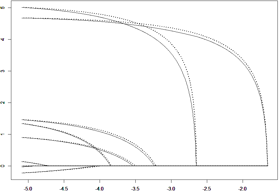
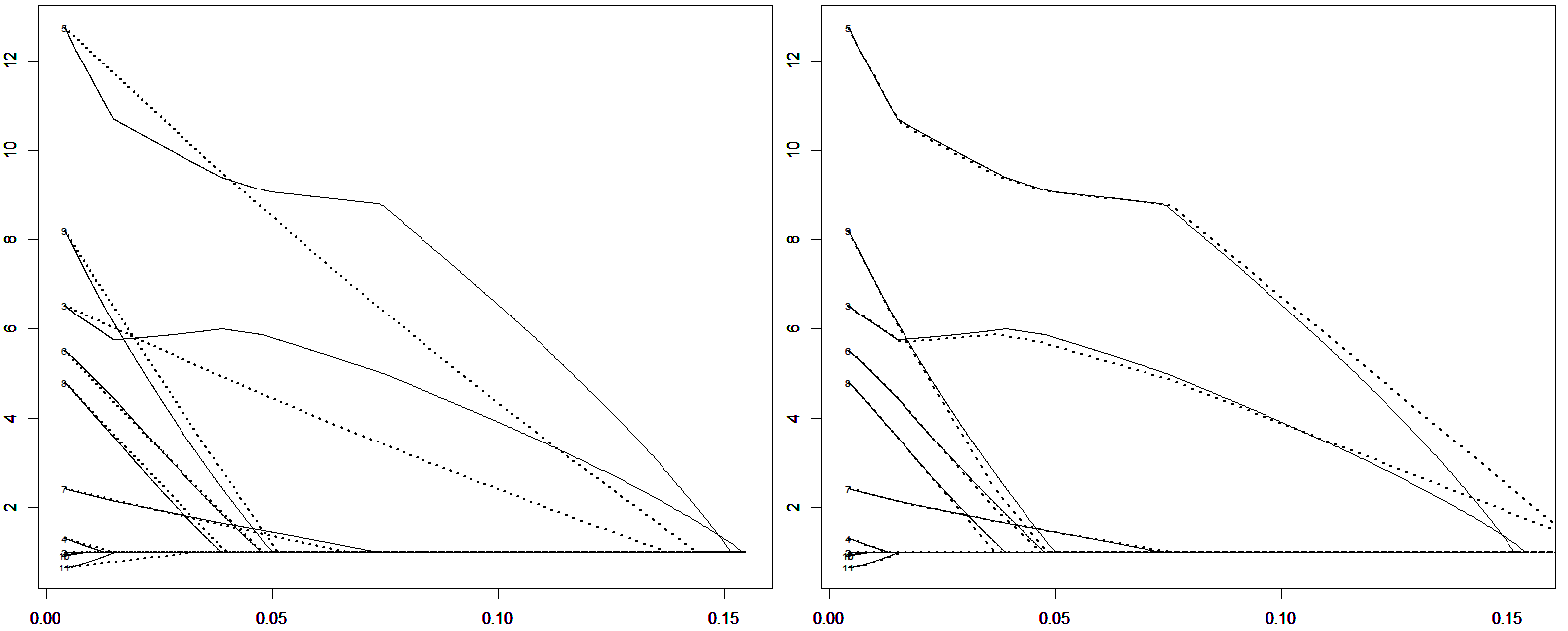
Refer to caption
Figure 2: Example 1. Path of regression coefficients with respect to log(t). The correlation between predictors is weak and the path given by the exact solution with independent predictors is a good approximation of the result.
Refer to caption
Figure 3: Example 2. We plotted the exponential of the beta coefficients with respect to t. On the left side by the assumption of no correlation, on the right side with the correction due to the approximate path algorithm. In presence of stong correlations, the algorithm of the approximate path (described in previous subsection) gives better adjusted graphs.

The Figure 3 shows common features encountered with other examples. The path of the exponential of the coefficients shapes a set of piecewise linear functions and the algorithm remains efficient even if the number of predictors is high (150 for examples). It seems that there is no case of a path with a curve reappearing after a first canceling (due to a strong correlation between predictors with opposite signs of initial coefficients). Thus, the sets AiA_{i} in the algorithm do not have to be determined.

We notice that the accuracy of this path following algorithm can easily be increased by adding intermediate steps (in variable t). The main computing limitation being the matrix inversion, one could study the inner product (Gram) matrix for class 0 and reorder rows and columns to reveal patterns and form a block diagonal matrix. These blocks could result from a statistical study of the Gram matrix66 6 To that end, see the literature of the block clustering problem [11]. (finding the pairwise independent predictors) as well as from pharmacological assumptions (medical treatments also shape patterns). Thus, computational costs become a marginal problem and one can concentrate on the bias correction by adding priors related to temporal bias, under-reporting or the introduction of similarity modifying the RR matrix77 7 With a similarity matrix S∈ℳp×p​([0,1])S\in\mathcal{M}_{p\times p}([0,1]), the similarity is defined as follows: coefficient Rj​kR_{jk} becomes (1−Sj​k)​Rj​k+Sj​k​min⁡(pj,pk)(1-S_{jk})R_{jk}+S_{jk}\min(p_{j},p_{k})..

6 Conclusion and perspectives

The central novelty of this work is the introduction of a rescaled likelihood for the limit imbalanced logistic regression problem. The expression of this likelihood could have some connexions with the well-known likelihoods of the self-controlled case series method [28] and of the proportional hazards model [4] used in epidemiology.

Most results exposed for binary data can be extented to other data types. However, simulations have been done only with binary data, having in mind the underlying applied problem of pharmacovigilance. The new estimate is always very close to the initial MLE because data are located on the vertexes of the hypercube and then one another ”close”. A convergence study of all possible existing algorithms for the primal and dual problems could be performed with different class imbalances and an evaluation of the first order term.

The variance reduction is a central issue that has to be treated in a Bayesian framework. Whereas the prior to add in the standard logistic regression is unclear, the rescaled likelihood takes a well-adapted form for exponential priors. We considered model selection using the BIC and the lasso to answer this question. Due to binary data, the lasso regularization problem became easier to understand in our limit imbalanced case: we found many precise estimators. Piecewise logarithmic approximate paths are built by an effective path following procedure which determines step by step the vanishing time of each path, do not use any loops as in coordinate descent algorithms and computes expressions only involving non-zero data. Moreover, this algorithm can take into account the correlation structure between predictors to further shrink computational costs. The values for N¯1\overline{N}^{1}, n¯0\overline{n}^{0} and for matrix RR could be shifted in order to incorporate absolute bias, temporal bias, under-reporting and similarity or correlation corrections.

7 A pharmacovigilance project?

Within this paper, we have had in mind the pharmacovigilance context as this work was carried out in parallel of a one-year engineering job at the French National Institute of Health and Medical Research88 8 B2PHI laboratory UMR 1181, INSERM, UVSQ, Institut Pasteur, Villejuif 94807, France. We hope this article could contribute a little to the developement of mathematical tools for pharmacovigilance purposes. The science of drug safety at a postmarketing level is nearly non-existent in France as in many other countries: the reporting process of spontaneous reports is inadequate and resulting databases are badly processed with unadapted tools. Public health scandals related to medication are steadily increasing and the spotlights are turned towards big pharmaceutical companies while patient associations should firstly require public authorities to establish a modern drug safety structure. To that end, the statistical community has a major role to play by proposing trustworthy decision-support tools, opposing science to political and financial influences. Creating a useful tool was the guideline of this present work and the author hopes that other mathematicians will embrace the direction initiated by this article.

We would like to conclude by giving our opinion about the work that remains to be done to obtain an operational tool (in five points), hoping that it will inspire epidemiologists.

1) Building priors related to bias (temporal bias, under-reporting…) with the help of pharmacologists. 2) Developing the proposed regularization algorithms evaluating their complexity and accuracy levels. 3) Introducing simple indicators to control the quality of the limit approximation. 4) Working on path visualization and new indicators (that are not thresholds). 5) Evaluating the obtained tool in the hands of pharmacologists (the use of reference sets is, to our mind, inadequate).

Acknowlegment

I would like to deeply thank Laetitia Comminges from the Paris-Dauphine University for relevant comments that greatly improved the manuscript. I also thank my colleague Mohammed Sedki from the INSERM laboratory of Villejuif for his constant encouragement to complete this work.

Appendix A Exact solutions

We give a collection of examples consisting in simple solutions of the equation (2.3).

A.1 No intercept

If there is no intercept and no interaction between the regressors, the matrix I\mathrm{I} equals the identity matrix 𝕀p\mathbb{I}_{p} and

β1=log⁡(n11n10),…,βp=log⁡(np1np0).\beta_{1}=\log\left(\frac{n_{1}^{1}}{n_{1}^{0}}\right)\,,\quad...\quad,\,\beta_{p}=\log\left(\frac{n_{p}^{1}}{n_{p}^{0}}\right)\,.

If one row contains other ones, the inverse matrix is the same matrix with the added ones transformed into its opposite.

A.2 Intercept

If the square matrix Ip+1\mathrm{I}_{p+1} is the following

Ip+1=(10⋯⋯010⋯00⋱⋱⋱⋱010⋯01),thenIp+1−1=(10⋯⋯0−110⋯00⋱⋱⋱⋱0−10⋯01)\mathrm{I}_{p+1}=\begin{pmatrix}1&0&\cdots&\cdots&0\\ \vdots&1&0&\cdots&0\\ \vdots&0&\ddots&\ddots&\vdots\\ \vdots&\vdots&\ddots&\ddots&0\\ 1&0&\cdots&0&1\\ \end{pmatrix}\,,\quad\hbox{then}\quad\mathrm{I}_{p+1}^{-1}=\begin{pmatrix}1&0&\cdots&\cdots&0\\ -1&1&0&\cdots&0\\ \vdots&0&\ddots&\ddots&\vdots\\ \vdots&\vdots&\ddots&\ddots&0\\ -1&0&\cdots&0&1\\ \end{pmatrix}

for the inverse matrix, so that the β\beta coefficients take the form

β0=log(n01n00),β1=log(n11n10n00n01),…,βp=log(np1np0n00n01).\beta_{0}=\log\left(\frac{n_{0}^{1}}{n_{0}^{0}}\right)\,,\quad\beta_{1}=\log\left(\frac{n_{1}^{1}}{n_{1}^{0}}\frac{n_{0}^{0}}{n_{0}^{1}}\right)\,,\quad...\quad,\,\beta_{p}=\log\left(\frac{n_{p}^{1}}{n_{p}^{0}}\frac{n_{0}^{0}}{n_{0}^{1}}\right)\,.

A.3 Intercept with one correlation

The first row of the following matrix

Ip+1=(1?⋯⋯?10⋯00⋱⋱⋱⋱010⋯01)\mathrm{I}_{p+1}=\begin{pmatrix}1&?&\cdots&\cdots&?\\ \vdots&1&0&\cdots&0\\ \vdots&0&\ddots&\ddots&\vdots\\ \vdots&\vdots&\ddots&\ddots&0\\ 1&0&\cdots&0&1\\ \end{pmatrix}

definies the set K={j∈{0,…,p},I1​j=1}K=\{j\in\{0,...,p\}\,,\,\mathrm{I}_{1j}=1\}. The case #​J=2\#J=2 is left out because it does not coincide with a non-singular matrix. The case #​J=1\#J=1 corresponds to the previous example. The easiest way to solve this example is to look at initial equations (2.1). We write down the p+1p+1 equations, where only the first one has a different form:

∑i=0p(ni1−ni0)=∑i=1p(ni1+ni0)​tanh⁡(β0+βi2)+(n01+n00)​tanh⁡(12​∑j∈Kβj)\sum_{i=0}^{p}(n_{i}^{1}-n_{i}^{0})=\sum_{i=1}^{p}(n_{i}^{1}+n_{i}^{0})\tanh(\frac{\beta_{0}+\beta_{i}}{2})+(n_{0}^{1}+n_{0}^{0})\tanh(\frac{1}{2}\sum_{j\in K}\beta_{j})

and for k∈{1,…,p}k\in\{1,...,p\},

(nk1−nk0)+1k∈K​(n01−n00)=(nk1+nk0)​tanh⁡(β0+βk2)+1k∈K​(n01+n00)​tanh⁡(12​∑j∈Kβj).(n_{k}^{1}-n_{k}^{0})+1_{k\in K}(n_{0}^{1}-n_{0}^{0})=(n_{k}^{1}+n_{k}^{0})\tanh(\frac{\beta_{0}+\beta_{k}}{2})+1_{k\in K}(n_{0}^{1}+n_{0}^{0})\tanh(\frac{1}{2}\sum_{j\in K}\beta_{j})\,. (A.1)

Subtracting all the pp equations to the first one, we obtain

(1−#​K)​(n01−n00)=(1−#​K)​(n01+n00)​tanh⁡(12​∑j∈Kβj),(1-\#K)(n_{0}^{1}-n_{0}^{0})=(1-\#K)(n_{0}^{1}+n_{0}^{0})\tanh(\frac{1}{2}\sum_{j\in K}\beta_{j}),\,

which can be used to simplify equations (A.1) into

(nk1−nk0)=(nk1+nk0)​tanh⁡(β0+βk2).(n_{k}^{1}-n_{k}^{0})=(n_{k}^{1}+n_{k}^{0})\tanh(\frac{\beta_{0}+\beta_{k}}{2})\,.

Finally, we have

exp⁡(∑j∈Kβj)=n01n00andexp⁡(β0+βk)=nk1nk0,k∈{1,…,p},\exp(\sum_{j\in K}\beta_{j})=\frac{n_{0}^{1}}{n_{0}^{0}}\quad\hbox{and}\quad\exp(\beta_{0}+\beta_{k})=\frac{n_{k}^{1}}{n_{k}^{0}}\,,\quad k\in\{1,...,p\}\,,

so that we deduce the following closed form for the β\beta coefficients

exp⁡(β0)=(n00n01​∏j∈J,j≠0(nj1nj0))1#​J−2,\exp(\beta_{0})=\left(\frac{n_{0}^{0}}{n_{0}^{1}}\prod_{j\in J,\,j\neq 0}\left(\frac{n_{j}^{1}}{n_{j}^{0}}\right)\right)^{\frac{1}{\#J-2}}\,,
exp⁡(βi)=ni1ni0​(n01n00​∏j∈J,j≠0nj0nj1)1#​J−2,i∈{1,…,p}.\exp(\beta_{i})=\frac{n_{i}^{1}}{n_{i}^{0}}\left(\frac{n_{0}^{1}}{n_{0}^{0}}\prod_{j\in J,\,j\neq 0}\frac{n_{j}^{0}}{n_{j}^{1}}\right)^{\frac{1}{\#J-2}}\,,\quad i\in\{1,...,p\}\,.

Notice that the regression coefficients behave in a very unpredictable way. It is sufficient to see that on an example with p=2p=2 and #​J=3\#J=3. The matrix I\mathrm{I} is

(111110101),\begin{pmatrix}1&1&1\\ 1&1&0\\ 1&0&1\\ \end{pmatrix}\,,

and we have

exp⁡(β0)=n00n01​n11​n21n10​n20,exp⁡(β1)=n01n00​n20n21,exp⁡(β2)=n01n00​n10n11.\exp(\beta_{0})=\frac{n_{0}^{0}}{n_{0}^{1}}\frac{n_{1}^{1}n_{2}^{1}}{n_{1}^{0}n_{2}^{0}}\,,\quad\exp(\beta_{1})=\frac{n_{0}^{1}}{n_{0}^{0}}\frac{n_{2}^{0}}{n_{2}^{1}}\,,\quad\exp(\beta_{2})=\frac{n_{0}^{1}}{n_{0}^{0}}\frac{n_{1}^{0}}{n_{1}^{1}}\,.

The first intuition is to think that coefficients β1\beta_{1} and β2\beta_{2} do depend on the couples (n10,n11)(n_{1}^{0},n_{1}^{1}) and (n20,n21)(n_{2}^{0},n_{2}^{1}) respectively, but it is not the case!

A.4 Stairs

With

Ip+1=(10⋯01⋱⋱⋱⋱01⋯11),we findIp+1−1=(10⋯⋯0−1⋱⋱0⋱⋱⋱⋱⋱⋱00⋯0−11)\mathrm{I}_{p+1}=\begin{pmatrix}1&0&\cdots&0\\ 1&\ddots&\ddots&\vdots\\ \vdots&\ddots&\ddots&0\\ 1&\cdots&1&1\\ \end{pmatrix}\,,\quad\hbox{we find}\quad\mathrm{I}_{p+1}^{-1}=\begin{pmatrix}1&0&\cdots&\cdots&0\\ -1&\ddots&\ddots&&\vdots\\ 0&\ddots&\ddots&\ddots&\vdots\\ \vdots&\ddots&\ddots&\ddots&0\\ 0&\cdots&0&-1&1\\ \end{pmatrix}

and then

β0=log⁡(n01n00),βi=log⁡(ni1ni0​ni−10ni−11),i∈{1,…,p}.\beta_{0}=\log\left(\frac{n_{0}^{1}}{n_{0}^{0}}\right)\,,\quad\beta_{i}=\log\left(\frac{n_{i}^{1}}{n_{i}^{0}}\frac{n_{i-1}^{0}}{n_{i-1}^{1}}\right)\,,\quad i\in\{1,...,p\}\,.

Appendix B Proof of Proposition 3.1.

The result is proved with a succession of Taylor expansions of degree 11 or 22 in 1/s1/s. We use

tanh⁡(x2)=−1+2​ex−2​e2​x+o⁡(e2​x),\tanh\left(\frac{x}{2}\right)=-1+2e^{x}-2e^{2x}+o(e^{2x})\,,

then with (2.2), we have

I1T​n1=I1T​n1​eI1​β+I0T​n0​eI0​β−(I1T​n1​e2​I1​β+I0T​n0​e2​I0​β)+o⁡(|n|​e2​β0).I_{1}^{T}n^{1}=I_{1}^{T}n^{1}e^{I_{1}\beta}+I_{0}^{T}n^{0}e^{I_{0}\beta}-\left(I_{1}^{T}n^{1}e^{2I_{1}\beta}+I_{0}^{T}n^{0}e^{2I_{0}\beta}\right)+o(|n|\,e^{2\beta_{0}})\,. (B.1)

The first equation of this system gives

|n1|=∑ni1​e(I1​β)i+∑ni0​e(I0​β)i−(∑ni1​e2​(I1​β)i+∑ni0​e2​(I0​β)i)+o⁡(|n|​e2​β0),|n^{1}|=\sum n^{1}_{i}e^{(I_{1}\beta)_{i}}+\sum n^{0}_{i}e^{(I_{0}\beta)_{i}}-\left(\sum n^{1}_{i}e^{2(I_{1}\beta)_{i}}+\sum n^{0}_{i}e^{2(I_{0}\beta)_{i}}\right)+o(|n|\,e^{2\beta_{0}})\,,

therefore, using notations introduced in the proposition,

e2​β0​(n21+s​n20)−eβ0​(n11+s​n10)+1−o⁡(1s)=0,e^{2\beta_{0}}\left(n_{2}^{1}+s\,n_{2}^{0}\right)-e^{\beta_{0}}\left(n_{1}^{1}+s\,n_{1}^{0}\right)+1-o(\frac{1}{s})=0\,,

and

eβ0=12​n11+s​n10n21+s​n20−12​n11+s​n10n21+s​n20​1−4​(1−o​(1s))​n21+s​n20(n11+s​n10)2.e^{\beta_{0}}=\frac{1}{2}\frac{n_{1}^{1}+s\,n_{1}^{0}}{n_{2}^{1}+s\,n_{2}^{0}}-\frac{1}{2}\frac{n_{1}^{1}+s\,n_{1}^{0}}{n_{2}^{1}+s\,n_{2}^{0}}\sqrt{1-4\left(1-o(\frac{1}{s})\right)\frac{n_{2}^{1}+s\,n_{2}^{0}}{(n_{1}^{1}+s\,n_{1}^{0})^{2}}}\,.

The coefficient ss is defined as s=|n0||n1|s=\frac{|n^{0}|}{|n^{1}|}. Now we have to find the Taylor expansion of eβ0e^{\beta_{0}} of degree two in 1/s1/s and reinject it in (B.1). We have

n21+s​n20(n11+s​n10)2=n21+s​n20s2​(n10)2​1(n11s​n10+1)2=n21+s​n20s2​(n10)2​(1−2​n11s​n10+o⁡(1s))\frac{n_{2}^{1}+s\,n_{2}^{0}}{(n_{1}^{1}+s\,n_{1}^{0})^{2}}=\frac{n_{2}^{1}+s\,n_{2}^{0}}{s^{2}(n_{1}^{0})^{2}}\frac{1}{(\frac{n_{1}^{1}}{sn_{1}^{0}}+1)^{2}}=\frac{n_{2}^{1}+s\,n_{2}^{0}}{s^{2}(n_{1}^{0})^{2}}\left(1-2\frac{n_{1}^{1}}{sn_{1}^{0}}+o(\frac{1}{s})\right)
=1s​n20(n10)2+1s2​(n21(n10)2−2​n11​n20(n10)3)+o⁡(1s2),=\frac{1}{s}\frac{n_{2}^{0}}{(n_{1}^{0})^{2}}+\frac{1}{s^{2}}\left(\frac{n_{2}^{1}}{(n_{1}^{0})^{2}}-2\frac{n_{1}^{1}n_{2}^{0}}{(n_{1}^{0})^{3}}\right)+o(\frac{1}{s^{2}})\,,

and

1−4​(1−o⁡(1s))​(1s​n20(n10)2+1s2​(n21(n10)2−2​n11​n20(n10)3)+o⁡(1s2))\sqrt{1-4\left(1-o(\frac{1}{s})\right)\left(\frac{1}{s}\frac{n_{2}^{0}}{(n_{1}^{0})^{2}}+\frac{1}{s^{2}}\left(\frac{n_{2}^{1}}{(n_{1}^{0})^{2}}-2\frac{n_{1}^{1}n_{2}^{0}}{(n_{1}^{0})^{3}}\right)+o(\frac{1}{s^{2}})\right)}
=1−4​(1s​n20(n10)2+1s2​(n21(n10)2−2​n11​n20(n10)3)+o⁡(1s2))=\sqrt{1-4\left(\frac{1}{s}\frac{n_{2}^{0}}{(n_{1}^{0})^{2}}+\frac{1}{s^{2}}\left(\frac{n_{2}^{1}}{(n_{1}^{0})^{2}}-2\frac{n_{1}^{1}n_{2}^{0}}{(n_{1}^{0})^{3}}\right)+o(\frac{1}{s^{2}})\right)}
=1−2​(1s​n20(n10)2+1s2​(n21(n10)2−2​n11​n20(n10)3+1​(n20)2(n10)4))+o⁡(1s2).=1-2\left(\frac{1}{s}\frac{n_{2}^{0}}{(n_{1}^{0})^{2}}+\frac{1}{s^{2}}\left(\frac{n_{2}^{1}}{(n_{1}^{0})^{2}}-2\frac{n_{1}^{1}n_{2}^{0}}{(n_{1}^{0})^{3}}+\frac{1(n_{2}^{0})^{2}}{(n_{1}^{0})^{4}}\right)\right)+o(\frac{1}{s^{2}})\,.

Therefore

eβ0=n11+s​n10n21+s​n20​(1s​n20(n10)2+1s2​(n21(n10)2−2​n11​n20(n10)3+1​(n20)2(n10)4)+o⁡(1s2))e^{\beta_{0}}=\frac{n_{1}^{1}+s\,n_{1}^{0}}{n_{2}^{1}+s\,n_{2}^{0}}\left(\frac{1}{s}\frac{n_{2}^{0}}{(n_{1}^{0})^{2}}+\frac{1}{s^{2}}\left(\frac{n_{2}^{1}}{(n_{1}^{0})^{2}}-2\frac{n_{1}^{1}n_{2}^{0}}{(n_{1}^{0})^{3}}+\frac{1(n_{2}^{0})^{2}}{(n_{1}^{0})^{4}}\right)+o(\frac{1}{s^{2}})\right)
=n11+s​n10s​n20​(1−n21s​n20+o⁡(1s))​(1s​n20(n10)2+1s2​(n21(n10)2−2​n11​n20(n10)3+(n20)2(n10)4)+o⁡(1s2))=\frac{n_{1}^{1}+s\,n_{1}^{0}}{s\,n_{2}^{0}}\left(1-\frac{n_{2}^{1}}{sn_{2}^{0}}+o(\frac{1}{s})\right)\left(\frac{1}{s}\frac{n_{2}^{0}}{(n_{1}^{0})^{2}}+\frac{1}{s^{2}}\left(\frac{n_{2}^{1}}{(n_{1}^{0})^{2}}-2\frac{n_{1}^{1}n_{2}^{0}}{(n_{1}^{0})^{3}}+\frac{(n_{2}^{0})^{2}}{(n_{1}^{0})^{4}}\right)+o(\frac{1}{s^{2}})\right)
=(n10n20+1s​(n11n20−n21​n10(n20)2))​(1s​n20(n10)2+1s2​(n21(n10)2−2​n11​n20(n10)3+(n20)2(n10)4))+o⁡(1s2)=\left(\frac{n_{1}^{0}}{n_{2}^{0}}+\frac{1}{s}\left(\frac{n_{1}^{1}}{n_{2}^{0}}-\frac{n_{2}^{1}n_{1}^{0}}{(n_{2}^{0})^{2}}\right)\right)\left(\frac{1}{s}\frac{n_{2}^{0}}{(n_{1}^{0})^{2}}+\frac{1}{s^{2}}\left(\frac{n_{2}^{1}}{(n_{1}^{0})^{2}}-2\frac{n_{1}^{1}n_{2}^{0}}{(n_{1}^{0})^{3}}+\frac{(n_{2}^{0})^{2}}{(n_{1}^{0})^{4}}\right)\right)+o(\frac{1}{s^{2}})
eβ0=1s​n10+(1s​n10)2​(n20n10−n11)+o⁡(1s2).e^{\beta_{0}}=\frac{1}{s\,n_{1}^{0}}+\left(\frac{1}{s\,n_{1}^{0}}\right)^{2}\left(\frac{n_{2}^{0}}{n_{1}^{0}}-n_{1}^{1}\right)+o(\frac{1}{s^{2}})\,.

The system of equations (B.1) without its first equation is

N¯1=𝙸1T​n1|n1|=eβ0​(𝕟𝟙𝟙+s​𝕟𝟙𝟘)−e2​β0​(𝕟𝟚𝟙+s​𝕟𝟚𝟘)+o⁡(1s)\overline{N}^{1}=\frac{\mathtt{I}_{1}^{T}n^{1}}{|n^{1}|}=e^{\beta_{0}}\left(\mathbb{n_{1}^{1}}+s\,\mathbb{n_{1}^{0}}\right)-e^{2\beta_{0}}\left(\mathbb{n_{2}^{1}}+s\,\mathbb{n_{2}^{0}}\right)+o(\frac{1}{s})

and we use the previous expression for eβ0e^{\beta_{0}}:

N¯1=(1s​n10+(1s​n10)2​(n20n10−n11))​(𝕟𝟙𝟙+s​𝕟𝟙𝟘)−(1s​n10)2​(𝕟𝟚𝟙+s​𝕟𝟚𝟘)+o⁡(1s)\overline{N}^{1}=\left(\frac{1}{s\,n_{1}^{0}}+\left(\frac{1}{s\,n_{1}^{0}}\right)^{2}\left(\frac{n_{2}^{0}}{n_{1}^{0}}-n_{1}^{1}\right)\right)\left(\mathbb{n_{1}^{1}}+s\,\mathbb{n_{1}^{0}}\right)-\left(\frac{1}{s\,n_{1}^{0}}\right)^{2}\left(\mathbb{n_{2}^{1}}+s\,\mathbb{n_{2}^{0}}\right)+o(\frac{1}{s})
N¯1=𝕟𝟙𝟘n10+1s​(n20(n10)2​[𝕟𝟙𝟘n10−𝕟𝟚𝟘n20]+n11n10​[𝕟𝟙𝟙n11−𝕟𝟙𝟘n10])+o⁡(1s)\overline{N}^{1}=\frac{\mathbb{n_{1}^{0}}}{n_{1}^{0}}+\frac{1}{s}\left(\frac{n_{2}^{0}}{(n_{1}^{0})^{2}}\left[\frac{\mathbb{n_{1}^{0}}}{n_{1}^{0}}-\frac{\mathbb{n_{2}^{0}}}{n_{2}^{0}}\right]+\frac{n_{1}^{1}}{n_{1}^{0}}\left[\frac{\mathbb{n_{1}^{1}}}{n_{1}^{1}}-\frac{\mathbb{n_{1}^{0}}}{n_{1}^{0}}\right]\right)+o(\frac{1}{s})

or

N¯1+1s​(𝕟𝟚𝟘(n10)2−𝕟𝟙𝟙n10)=𝕟𝟙𝟘n10​(1+1s​(n20(n10)2−n11n10))+o⁡(1s).\overline{N}^{1}+\frac{1}{s}\left(\frac{\mathbb{n_{2}^{0}}}{(n_{1}^{0})^{2}}-\frac{\mathbb{n_{1}^{1}}}{n_{1}^{0}}\right)=\frac{\mathbb{n_{1}^{0}}}{n_{1}^{0}}\left(1+\frac{1}{s}\left(\frac{n_{2}^{0}}{(n_{1}^{0})^{2}}-\frac{n_{1}^{1}}{n_{1}^{0}}\right)\right)+o(\frac{1}{s})\,.

Then, using again a Taylor expansion,

𝕟𝟙𝟘n10=N¯1+1s​(𝕟𝟚𝟘−N¯1​n20(n10)2−𝕟𝟙𝟙−N¯1​n11n10)+o⁡(1s)\frac{\mathbb{n_{1}^{0}}}{n_{1}^{0}}=\overline{N}^{1}+\frac{1}{s}\left(\frac{\mathbb{n_{2}^{0}}-\overline{N}^{1}n_{2}^{0}}{(n_{1}^{0})^{2}}-\frac{\mathbb{n_{1}^{1}}-\overline{N}^{1}n_{1}^{1}}{n_{1}^{0}}\right)+o(\frac{1}{s})

or

𝕟𝟙𝟘n10−N¯1=1s​(n20(n10)2​(𝕟𝟚𝟘n20−N¯1)−n11n10​(𝕟𝟙𝟙n11−N¯1))+o⁡(1s).\frac{\mathbb{n_{1}^{0}}}{n_{1}^{0}}-\overline{N}^{1}=\frac{1}{s}\left(\frac{n_{2}^{0}}{(n_{1}^{0})^{2}}\left(\frac{\mathbb{n_{2}^{0}}}{n_{2}^{0}}-\overline{N}^{1}\right)-\frac{n_{1}^{1}}{n_{1}^{0}}\left(\frac{\mathbb{n_{1}^{1}}}{n_{1}^{1}}-\overline{N}^{1}\right)\right)+o(\frac{1}{s})\,.

Appendix C Path simulations

In the following graphs, the dotted lines are obtained by the exact path corresponding to Theorem 4.1 for examples 1 and 2, Theorem 4.2 for examples 3 and 4 and the inclusion case for examples 5 and 6. The solid lines are always given by a coordinate descent algorithm for the standard logistic regression. We change the scale for tt (by a linear rescaling) in order to have to same max⁡(t)\max(t) (see (5.1)) for the exact and algorithmic paths.

Refer to caption
Figure 4: Example 1. Independence and class imbalance. β0=−3\beta_{0}=-3 (|n0|/|n1|=17|n^{0}|/|n^{1}|=17).
Refer to caption
Figure 5: Example 2. Independence and no class imbalance. β0=0\beta_{0}=0 (|n0|/|n1|=1.5|n^{0}|/|n^{1}|=1.5).
Refer to caption
Figure 6: Example 3. Orthogonality and class imbalance. β0=−3\beta_{0}=-3 (|n0|/|n1|=15|n^{0}|/|n^{1}|=15).
Refer to caption
Figure 7: Example 4. Orthogonality and no class imbalance. β0=0\beta_{0}=0 (|n0|/|n1|=0.8|n^{0}|/|n^{1}|=0.8).
Refer to caption
Figure 8: Example 5. Inclusion and class imbalance. β0=−3\beta_{0}=-3 (|n0|/|n1|=15|n^{0}|/|n^{1}|=15).
Refer to caption
Figure 9: Example 6. Inclusion and no class imbalance. β0=0\beta_{0}=0 (|n0|/|n1|=0.8|n^{0}|/|n^{1}|=0.8).

References

  • [1] Ahmed Ismail, Pariente Antoine, Tubert-Bitter Pascale (2016) Class-imbalanced subsampling lasso algorithm for discovering adverse drug reactions. Statistical Methods in Medical Research.
  • [2] Beziz et al. (2016) Spontaneous adverse drug reaction reporting in France: A retrospective analysis of reports made to the French medicines agency from 2002 to 2014. Revue d’Épidémiologie et de Santé Publique, 64.
  • [3] Caster et al. (2010) Large-Scale Regression-Based Pattern Discovery: The Example of Screening the WHO Global Drug Safety Database. Stat. Anal. Data Min., 3, no. 4, 197–208.
  • [4] Cox David Roxbee (1975) Partial likelihood. Biometrika, 62, no. 2, 269–276.
  • [5] Efron Bradley, Hastie Trevor, Johnstone Iain, Tibshirani Robert (2004) Least angle regression. Annals of statistics, 32, no. 2, 407–499.
  • [6] Elrahman Shaza, Abraham Ajith (2013) A Review of Class Imbalance Problem. Journal of Network and Innovative Computing., 1, 332–340.
  • [7] Firth David (1993) Bias reduction of maximum likelihood estimates. Biometrika, 80, no. 1, 27–38.
  • [8] Fithian William, Hastie Trevor. (2014) Local case-control sampling: efficient subsampling in imbalanced data sets. Ann. Statist., 42, no. 5, 1693–1724.
  • [9] Friedman Jerome, Hastie Trevor, Tibshirani Rob (2010) Regularization Paths for Generalized Linear Models via Coordinate Descent. Journal of Statistical Software, 33, no. 1, 1–22.
  • [10] Friedman Jerome, Hastie Trevor, Höfling Holger, Tibshirani Robert (2007) Regularization Paths for Generalized Linear Models via Coordinate Descent. Annals of Applied Statistics, 1, no. 2, 302–332.
  • [11] Govaert Gérard, Nadif Mohamed (2008) Block clustering with Bernoulli mixture models: comparison of different approaches. Comput. Statist. Data Anal., 52, no. 6, 3233–3245.
  • [12] Guo Xinjian et al. (2008) On the Class Imbalance Problem. Proceedings ot the Fourth International Conference on Natural Computation. 4, 192–201.
  • [13] Harpaz et al. (2013) Performance of pharmacovigilance signal-detection algorithms for the FDA adverse event reporting system. Clin Pharmacol. Ther., 6
  • [14] Hiriart-Urruty Jean-Baptiste (1981) A note on the Legendre-Fenchel transform of convex composite functions. Nonsmooth Mechanics and Analysis. Adv. Mech. Math. Springer, New York, 12, 35–46.
  • [15] Jeffreys Harold. (1946) An invariant form for the prior probability in estimation problems. Proc. Roy. Soc. London. Ser. A., 186, 453–461.
  • [16] Ki Hang Kim (1982) Boolean matrix theory and applications. Monographs and textbooks in pure and applied mathematics. ISBN-13: 978-0824717889
  • [17] Lipovetsky Stan (2015) Analytical closed-form solution for binary logit regression by categorical predictors. J. Appl. Stat., 42, no. 1, 37–49.
  • [18] Madigan David, Ryan Patrick, Simpson Shawn, Zorych Ivan (2011) Bayesian methods in pharmacovigilance. With discussion by William DuMouchel. Oxford Univ. Press, Bayesian statistics 9, 421–438.
  • [19] Mantel, N. and Haenszel, W. (1959) Statistical aspects of the analysis of data from retrospective studies of disease. J. Natl. Cancer Inst., 22, 719–748.
  • [20] Minka Thomas P. (2007) A comparison of numerical optimizers for logistic regression. URL: http://research.microsoft.com/en-us/um/people/minka/papers/logreg/
  • [21] Oommen Thomas et al. (2011) Sampling Bias and Class Imbalance in Maximum-likelihood Logistic Regression. Mathematical Geosciences., 43, no. 1, 99–120.
  • [22] Owen Art B. (2007) Infinitely Imbalanced Logistic Regression. J. Mach. Learn. Res., 8, 761–773.
  • [23] Rosset Saharon (2004). Following Curved Regularized Optimization Solution Paths. Advances in Neural Information Processing Systems. 17, 1153–1160.
  • [24] Rosset S. and Zhu J. (2007). Piecewise linear regularized solution paths. The Annals of Statistics. 35, no. 3, 1012–1030.
  • [25] Saint-Raymond Laure (2009). Hydrodynamic Limits of the Boltzmann Equation. Springer. Lecture Notes in Mathematics. ISBN: 978-3-540-92846-1
  • [26] Schwarz Gideon (1978) Estimating the dimension of a model. The Annals of Statistics, 6, no. 2, 461–464.
  • [27] Silvapulle Mervyn J. (1981) On the Existence of Maximum Likelihood Estimators for the Binomial Response Models. J. Roy. Statist. Soc. Ser. B, 43, no. 3, 310–313.
  • [28] Simpson Shawn E, Madigan David, Zorych Ivan, Schuemie Martijn J., Ryan Patrick B., Suchard Marc A. (2013) Multiple self-controlled case series for large-scale longitudinal observational databases. Biometrics, 69, no. 4, 893–902.
  • [29] Tibshirani Robert (1996) Regression shrinkage and selection via the lasso. J. Roy. Statist. Soc. Ser. B, 58, no. 1, 267–288.
  • [30] Yu Hsiang-Fu, Huang Fang-Lan, Lin Chih-Jen (1981) Dual coordinate descent methods for logistic regression and maximum entropy models. Mach. Learn., 85, no. 1-2, 41–75.
  • [31] Zou Hui, Hastie Trevor (2005) Regularization and variable selection via the elastic net. J. R. Stat. Soc. Ser. B Stat. Methodol., 67, no. 2, 301–320.