![[Uncaptioned image]](1703.08819v1/torver.png)
UNIVERSITÀ DEGLI STUDI DI ROMA “TOR VERGATA”
Dipartimento di Matematica
Dottorato di Ricerca in Matematica
Ciclo XXVIII
New normal form approaches
adapted to the Trojan problem
Rocío Isabel PÁEZ
Relatore: Dr. Ugo LOCATELLI
Coordinatore del corso di dottorato:
Prof. Carlo SINESTRARI
- Anno Accademico 2014/2015 -
Roma, Italia
To my own personal Jesus
Preface
The present thesis resumes the research carried out in the framework
of the author’s Ph.D. program, supported by
the Marie Curie Training Network ’Astronet-II The
Astrodynamics Network’ (PITN-GA-2011-289240), under the supervision of
Dr. Ugo Locatelli. The results here presented are based on original research
developed by the author. Part of the results are
contained in the following publications:
Páez, R.I., Locatelli, U., (2014)
Design
of maneuvers based on new normal form approximations: the case
study of the CPRTBP, ICNPAA 2014 Proceedings, AIP Conf.
Proceedings 1637, p. 776.
Efthymiopoulos, C., Páez, R.I., (2014)
Modeling resonant Trojan motions in planetary systems,
Complex Planetary Systems, Proceedings IAU Symposium 310,
Z. Knezevic et A. Lemaitre, eds., p 70.
Páez, R.I., Efthymiopoulos, C., (2014)
Modeling Trojan dynamics: diffusion mechanisms through resonances,
Complex Planetary Systems, Proceedings IAU Symposium 310,
Z. Knezevic et A. Lemaitre, eds., p 96.
Páez, R.I., Efthymiopoulos, C., (2015)
Trojan
resonant dynamics, stability and chaotic diffusion, for parameters
relevant to exoplanetary systems, Celest. Mech. Dyn. Astron.
121, p. 776.
Páez, R.I., Locatelli, U., (2015)
Trojan
dynamics well approximated by a new Hamiltonian normal form,
Mon. Not. R. Astron. Soc. 453, p. 2177.
Páez, R.I., Locatelli, U., Efthymiopoulos, C.,
(2016)
The Trojan problem from a Hamiltonian perturbative
perspective, Gómez G., Masdemont J. (eds) Astrodynamics
Network AstroNet-II, Astrophysics and Space Science Proceedings
44, p. 193.
Páez, R.I., Locatelli, U., Efthymiopoulos, C., (2016)
New Hamiltonian expansions adapted to the Trojan problem
Celest. Mech. Dyn. Astron.
126, p. 516.
Páez, R.I. (2017)
Analytical boundary for effective stability domains of Trojan motions
(preprint).
Rocío Isabel Paez
e-mail: paez@mat.uniroma2.it
website: http://www.mat.uniroma2.it/~paez
Roma, February 2016.
Abstract
The main subject of this work is the study of the problem of the Trojan orbits from a perturbative Hamiltonian perspective. We face this problem by introducing first a novel Hamiltonian formulation, exploiting the well-differentiated temporal scales of the Trojan motion. The resulting Hamiltonian allows to separate the secular (very slow) component of the motion from the librating and fast degrees of freedom. This decompositon provides the foundation of a so-called Basic Hamiltonian model (), i.e. the part of the Hamiltonian for Trojan orbits independent of all secular angles. Our study shows that, up to some extent, the model successfully represents the features of the motion under more complete models, in a range of physical parameters relevant for dynamics in the Solar System or in extrasolar planetary systems.
We propose, then, two novel normal form schemes in order to analytically study the model . The first scheme takes into account the existence of a real singularity due to close encounters of the Trojan body with the primary, by avoiding any polynomial or trigonometric expansion for the librating angle. The second scheme exploits the fact that the Trojan orbits are highly asymmetric with respect to the libration center. We then analytically construct a so-called "asymmetric expansion", which extends the domain of the normal form series’ convergence with respect to the usual polynomial expansions around the stable Lagrangian points L4 or L5.
Both schemes are tested in detail in the framework of the Circular and Elliptic Restricted 3-Body Problems, focusing particularly on the analytical derivation of the location of secondary resonances embedded within the libration domain. Additionally, the second scheme provides an analytical estimation of the width of such resonances.
Finally, the thesis analyses the key usefulness of the model, pointing out the possibility for straightforward extensions allowing to include additional bodies (Restricted Multi-Planet Problem), and/or Trojan motions in 3D space.
Chapter 1 Introduction
This thesis is devoted to the study of the problem of the librational motion in the neighborhood of the celebrated triangular points found by Lagrange (1772) in the framework of the gravitational problem of three bodies. This problem has a wide spectrum of applications. In our Solar System, the moving bodies represent, for example, the so-called Trojan asteroids located close to the Lagrangian points of the Sun-Jupiter system. Trojan asteroids were also found near other planets in our solar system. It has been conjectured (see references in Sect. 1.4) that Trojan planets or asteroids should exist in extrasolar planetary systems as well.
In his seminal work Les Méthodes Nouvelles de la Mécanique Celeste [100], H. Poincaré emphasized the use of the Hamiltonian method in the problems of Celestial Mechanics and in dynamical astronomy in general. The Hamiltonian formalism is based on the use of sets of variables subject to a particular class of transformations, called canonical or symplectic. Such transformations lend themselves quite conveniently to developing perturbative series solutions of the equations of motion for, e.g., celestial bodies. The associated approach has become known in the mathematical literature as the method of Hamiltonian normal forms. In the present thesis, we exploit the method of normal forms in the context of Trojan dynamics.
In this chapter, we briefly summarize some basic notions of the canonical formalism as well as the relevant concepts of the problem of Trojan motions, emphasizing those aspects which are needed in subsequent chapters. Finally, we describe the goal and structure of the present dissertation.
1.1 Hamiltonian Mechanics
1.1.1 Hamilton’s equations
A system of ordinary differential equations of the type (for )
| (1.1) |
is said to be in Hamiltonian form if there exists a function such that the equations (1.1) can be rewritten as
| (1.2) |
The function is called the Hamiltonian of the system and the equations of motion in (1.2) are Hamilton’s equations ([5], [55]). The variables are called canonical momenta and coordinates respectively. The space spanned by the canonical variables is called phase space. The system (1.2) is said to be of degrees of freedom (d.o.f.).
We call cyclic a coordinate that does not appear explicitely in the Hamiltonian function. In this case, the conjugate momentum is preserved. Taking into account Eq. (1.2), the total time derivative of the Hamiltonian is
| (1.3) |
Therefore, is constant in time as long as it does not depend explicitely on (autonomous Hamiltonian). The non autonomous systems are said to be of d.o.f. In fact, it is possible to extend the phase-space, by including an additional variable conjugate to the time , that gives a new Hamiltonian of d.o.f. preserved in time. Thus, all the results applicable to autonomous systems may be generalized to the non autonomous systems as well.
Let and be two generic functions of the generalized coordinates , , . The Poisson bracket between and is defined by
| (1.4) |
If we apply the Poisson bracket to and the Hamiltonian , we obtain
| (1.5) |
In words, the computation of the Poisson bracket gives the time evolution of any dynamical variable , i.e. a differentiable real function of the canonical coordinates , under the flow induced by the Hamiltonian . Applying this to the generalized coordinates, we can rewrite Hamilton’s equations as follows:
| (1.6) |
1.1.2 Canonical transformations
Let us consider a time-independent transformation of variables defined by the following (invertible) equations
| (1.7) |
If for any Hamiltonian function of the canonical conjugated variables , the new set of variables , satisfies Hamilton’s equations,
| (1.8) |
where the new Hamiltonian function is given by
| (1.9) |
then the transformation (1.8) is called canonical. In other words, a canonical transformation is a change of coordinates that preserves the form of Hamilton’s equations.
A straightforward way to check whether a transformation of the form (1.7) is canonical is based on the following property [4]: the transformation (1.7) is canonical if and only if it preserves the fundamental Poisson brackets,
| (1.10) |
for , .
Equations (1.10) can be used to check the canonical property when the transformation is given. However, they cannot be used directly in order to construct canonical transformations of the form (1.7). We now refer to two methods that do allow to construct them explicitly.
The first method is based on the construction of a generating function . This is a function depending on a particular combination of old/new momenta and coordinates. A common division distinguishes four classes: 1st class , if the generating functions depends on the old and new coordinates, i.e. ; 2nd class , if it depends on the old coordinates and new momenta, i.e. ; 3rd class if ; 4th class if . The canonical transformation equations are given by the corresponding derivatives of . For example, for an arbitrary choice of generating function of 2nd class, , it can be shown that the transformation equations
| (1.11) |
are canonical (see §1.2a of [71]), as long as they are invertible, e.g.
| (1.12) |
In an analogous way, we derive the transformations for the other classes of generating functions.
The second method consists of the use of Lie generating functions of the original canonical variables , and a parameter . The function generates a canonical transformation from old to new variables by means of Hamilton equations
| (1.13) |
and the new variables are related to the old variables by
| (1.14) |
assuming that and . Since it is derived from a Hamiltonian-like flow (induced by ), this transformation must be canonical.
The method of Lie generating functions is widely used in perturbation theory for producing near to identity canonical transformations ([60], [24]). An advantage of the Lie method is that it provides an explicit expression of the transformations , . On the contrary, the method based on the generating functions provides implicit formulæ which need to be inverted in order to obtain the explicit form of the transformation equations.
1.1.3 Action-angle variables
Let us consider a dynamical variable . If
| (1.15) |
then is called first integral of the Hamiltonan . We can immediately notice that if two dynamical variables and are first integrals, then is a first integral as well. In particular, in autonomous systems is a first integral of the Hamiltonian flow.
Let be an autonomous Hamiltonian of d.o.f. possessing a set of first integrals which satisfy the following properties: i. they are independent, i.e.
| (1.16) |
and ii. they form an involution system, i.e. they accomplish the property
| (1.17) |
Assume also that the hypersurfaces of constant energy are compact.
Under these conditions, the Liouville-Arnold-Jost theorem ([1],[62]) states that it is possible to locally construct a canonical transformation such that in the new variables the Hamiltonian acquires the form
| (1.18) |
In Eq. (1.18) all the coordinates , called the angles, are cyclic. The solution of Hamilton’s equations is then trivial, given by
| (1.19) |
where . The momenta are called the actions11 1 In general, the actions are defined only locally, e.g the pendulum admits different actions inside and outside the separatrix.. Their value along any particular orbit remains constant, while the temporal evolution of the angles is linear with frequency . A system of the above form is called Arnold-Liouville integrable. Figure 1.1 provides a schematic representation of the orbits in the phase-space defined by the action-angle variables. Since the evolution of the motion is given strictly by Eqs. (1.19), the orbit lies on an invariant torus , defined by the constant values of the actions . The uniform motion on the torus is given by the value of the angles according to Eq. (1.19). The orbits are called quasiperiodic if the frequencies are such that
| (1.20) |
A torus on which (1.20) holds is called non resonant. On the other hand, if there exist one or more combinations of integer values such that
| (1.21) |
the torus is called resonant. The commensurability between frequencies induces orbits lying on so-called lower-dimensional tori, i.e. tori of dimension lower than . If independent relations of the form (1.21) exist, the corresponding orbits lie in a -dimensional torus. Of particular importance is the case . Then, the corresponding orbits are -dimensional tori, called periodic orbits. In Fig. 1.1, the red orbit represents a case of periodic orbit. Every time when the orbit completes a period , its position in terms of is the same. Finally, a trivial consequence of the Liouville-Arnold-Jost theorem is that an autonomous Hamiltonian of 1 d.o.f. is integrable, since it has one first integral: the Hamiltonian itself.

1.1.4 Normal form theory for nearly-integrable systems
Most dynamical systems in nature are non integrable. H. Poincaré [100] emphasized the importance of systems for which the Hamiltonian function has the form
| (1.22) |
where is an integrable hamiltonian and is a fuction expandable as a convergent series in powers of . According to Poincaré, understanding the solutions of the systems of the form (1.22) constitutes the fundamental problem of dynamics. In particular, if the size of the perturbation to the integrable system is a small quantity, the system is called nearly integrable.
Although cases of strongly chaotic dynamics are easy to identify, nearly integrable dynamics is the most frequent case encountered in Solar System dynamics. In nearly integrable systems the solutions cannot be found in such explicit form as in integrable systems (like, for example, the Two-Body problem). However, quite precise approximate solutions can be obtained by employing the method of normal forms.
A normal form can be defined as a Hamiltonian function yielding a simple-to-analyse dynamics [32]. In general, this does not imply that we can reduce a non-integrable Hamiltonian to an integrable one. However, we can approximate it by a normal form with properties that render its study simpler. This normal form is produced after implementing a set of conveniently chosen canonical transformations to the variables of the original Hamiltonian.
Let us consider a canonical transformation of the form (1.7). In the normal form method, we look for a canonical transformation such that, after applying the change of variables, the Hamiltonian is decomposed in the form
| (1.23) |
with . The term in (1.23) called the normal form, while is called the remainder. The importance of the latter lies on the fact that it tells us how different is the dynamics of the original Hamiltonian with respect to the normal form. In practice, while applying a sequence of canonical transformations, we must control the growth of the size of the remainder. Most so-called normalizing schemes, i.e. sequences of canonical transformations, are designed in order to keep appropriate control on this growth [53], [32].
To obtain the normalized Hamiltonian, we need to produce a sequence of near-identity canonical transformations. To this end, we discuss now the technique of Lie series. Let us consider an arbitrary function . As described in (1.13), the flow produced by Hamilton’s equations using as the hamiltonian function, is given by
| (1.24) |
Let and denote the solutions in time, with initial conditions , . The transformation , viewed as a mapping, is a canonical transformation for any arbitrary time [4]. In this sense, can be considered as a function from which we can obtain infinitely many canonical transformations, by solving Hamilton’s equations for differents values of the time . Accordingly, can be thought of as a parameter generating the whole family of canonical transformations induced by (the parameter used in Eq. 1.14).
In general, we are not able to explicititely integrate Hamilton’s equations (1.24) for all times . However, for small, it is possible to obtain a solution of the initial value problem (1.24) through Taylor expansions. The key remark is that, from the equations of the flow (1.24) we can compute the time derivative of all orders for the canonical variables , , , as functions of the canonical variables themselves. For example,
| (1.25) | ||||
Thus, the second order time derivative of is expressed in terms of and partial derivatives of . This process can be generalized for all the variables and orders of the derivatives needed for a truncated Taylor series.
Let us define the Lie operator . According to (1.5), for a generic dynamical variable , we have
| (1.26) |
that corresponds to the time derivative of along a Hamiltonian flow induced by . Generalizing this notation for higher order derivatives we have
| (1.27) |
Now, we can construct the Taylor series for the solutions ,
| (1.28) | ||||
where and and . Replacing the Lie operator notation in Eqs. (1.28), we have
| (1.29) | |||
where and , and . The last equations correspond to the formal definition of a Lie series. As mentioned before, they provide a family of canonical transformations for any value of the time variable within their domain of convergence. The convergence of the series is discussed, e.g., in [53], [32]. Let us assume that and its derivatives are small enough so that the series are convergent for . Then, we have
| (1.30) | |||
which are the Lie canonical transformations from . Using the exponential operator
| (1.31) |
we re-express all the canonical transformations in a compact form
| (1.32) |
with the Lie exponential operator defined by
| (1.33) |
The following properties of the Lie series are relevant in practical computations:
i. the function can be chosen in a completely
arbitrary way. This gives the freedom to choose in order to ensure
that the transformed Hamiltonian acquires the normal form properties we
look for;
ii. in the computation of the
transformations (1.32), the only operations
involved are sums, products and derivatives, which are easy to
implement in an computer-algebraic program;
iii. considering a small quantity, Eq. (1.33)
implies that the Lie series generates a near-identity
transformation;
iv. the time derivative of any function under the Hamiltonian flow induced by is given by (1.26), hence
| (1.34) |
In other words, it is possible to find which form acquires the function after applying the transformation (1.32) without performing function compositions; instead we apply the corresponding Lie operator directly on [57], [53] (property known as the ’Exchange theorem’). This key argument allows to replace complicated compositions of functions by just trivial operations.
We now briefly discuss the algorithm of computation of a normal form via Lie series (for details see, e.g., [71]). Following [32], we introduce a convenient notation called ’book-keeping’, which allows to expose the normal form algorithm in a way easily transcribable to a computer-algebraic program. Let be a function of the canonical variables depending on one or more small parameters, like in Eq. (1.22). In some problems of Celestial Mechanics, such parameters can be the masses of the planets (divided by the mass of the Sun), eccentricities or inclinations, amplitudes of libration around particular equilibrium solutions, etc. Depending on the size of these parameters, in perturbation theory we encounter series expansions of of the form , where represents terms estimated as of ”-th order of smallness”. The value of can be chosen to be connected to the exponents of various small parameters by a specific rule, that we hereafter call the book-keeping rule. To formally account for this, we introduce in the notation a symbol , with numerical value equal to . Thus, in the sequel, a term with a factor in front is meant as a term estimated to be of -th order of smallness.
Returning to the normal form algorithm, let denote the initial Hamiltonian. At the first normalization step, we separate the terms of as follows
| (1.35) |
denotes the terms of the Hamiltonian which we choose to be in normal form at the zero-th order. All remaining terms should be assigned book-keeping order or higher. The choice of can have a certain degree of arbitrariness and different choices lead to different normalization schemes.
We now seek to determine a canonical transformation such that the Hamiltonian function, expressed in the new variables , is in normal form up to order . Let be the generating function accomplishing this transformation. Let us consider for a moment that was given. The Hamiltonian after applying the transformation reads
| (1.36) |
whose lowest order terms are
| (1.37) |
Replacing Eq. (1.37) in Eq. (1.35), we obtain
| (1.38) | ||||
If we define as a quantity of first order in (), we have
| (1.39) | ||||
Now we aim to produce a new Hamiltonian such that, at order , it contains only terms in normal form. To achieve so, the generating function must be defined so as to satisfy the equation
| (1.40) |
where are the terms of which are not in normal form, i.e. those we do not want to keep in . An equation like (1.40) is known as the homological equation. Its solution specifies the generating function . Then, implementing Eq. (1.36), we also find the now transformed Hamiltonian .
The solution of the homological equation can be found in a straighforward way, if the term is chosen in the initial step as
| (1.41) |
with , . A choice of the form (1.41) is possible when the variables are action-angle variables, and the problem under study has the structure of coupled nonlinear oscillators. By replacing each trigonometric function of the angles by
| (1.42) |
for (and similarly for ), the function can be written in the form
| (1.43) |
with . Substituting Eqs. (1.43) and (1.41) in the homological equation (1.40), we obtain the solution for the generating function
| (1.44) |
where . For the solution to exist, all denominators must be different from zero. This restriction limits our possible choice of functions , i.e. should contain no Fourier terms with wavevectors satisfying . Albeit not explicitely needed, in practice we exclude also the terms satisfying
from . In fact, the question of how to properly identify terms that generate small divisors is one of the most importants in normal form theory.
With the expression of the generating function , we finally obtain the new transformed Hamiltonian by applying the Lie series operator,
| (1.45) |
which, by construction, is in normal form up to order .
The above normalization step of the Hamiltonian can be generalized to any higher order. Let us consider the Hamiltonian , which we assume is in normal form up to order :
| (1.46) |
Some of the terms of , denoted as , are not in normal form, thus we want to eliminate them. As in Eq. (1.39), from the Lie series , we see that the only terms of order are those coming from and . Therefore, the corresponding homological equation for this step reads
| (1.47) |
which can be solved in the same way as Eq. (1.40). Applying the Lie series operator to
| (1.48) |
we obtain which, by construction, is in normal form up to , i.e.
| (1.49) |
where .
1.1.5 Linear and non-linear stability
Let us consider a system represented by a Hamiltonian function . Let be an equilibrium point of . Hamilton’s equations (1.2) for the equilibrium point yield
| (1.50) |
We define an orbit slightly displaced with respect to the equilibrium as
| (1.51) |
where is a vector whose components are all small quantities. If we replace Eq. (1.51) in Eqs. (1.2), and we keep only terms of first order around the equilibrium position, we produce the linearized system,
| (1.52) |
where the constant matrix contains the second derivatives of evaluated at the equilibrium point. The solutions to Eq. (1.52) are given by
| (1.53) |
where are the eigenvalues corresponding to , is the matrix whose columns are the eigenvectors of , and are constants of integration, in practice derived by the initial conditions [65].
According to the nature of the eigenvalues , the solutions are stable oscillations around the equilibrium point (all are imaginary), or present one or more unstable components (at least one of the has ). Thus, the linear stability of the motion in the vicinity of can be concluded only by the eigenvalues of the matrix . The latter are computed by solving the characteristic equation
| (1.54) |
with the identity matrix.
Linear stability around an equilibrium point does not guarantee also stability when terms of order higher than linear are retained in the variational equations. Higher order perturbations to the linear system may raise unstable trajectories, causing escapes. Additionally, some orbits that are quasiperiodic in the linear approach may not persist as such in the non-linear model.
We now briefly refer to some well-known approaches to the problem of nonlinear stability of the orbits in systems of the form (1.22). The so-called Kolmogorov-Arnold-Moser (KAM) theorem ([63], [91], [2]) examines the existence of quasiperiodic orbits when an integrable Hamiltonian system is disturbed by a sufficiently small Hamiltonian perturbation. Let us consider a system represented by Eq. (1.22), where the integrable part generates solutions of the form (1.19), with . Let us assume also that satisfies an appropriate non-degeneracy condition (see, e.g. [4]). The simplest such condition is that the gradients for , are linearly independent. The theorem states that, for a sufficiently small, a large (of order ) measure of the non resonant invariant tori of the unperturbed problem survive as deformed invariant tori, with the original frequencies, in the perturbed problem (§6.3 of [5], §2.3.5. of [19]). The preserved invariant tori are called KAM tori, and they are characterized by frequencies which are ’far from being resonant’, typically described by the diophantine condition
| (1.55) |
where is the integer vector .
In the case of a system of 2 d.o.f, the phase space is 4-dimensional and any trajectory evolves on an 3D isoenergetic surface. Thus, a KAM torus divides the phase space in two non-communicating parts, restricting the motion to one part or the other. This ensures the non linear stability for all the orbits confined in the interior of an invariant KAM torus. However, in systems of more than 2 d.o.f., the invariant tori do not isolate the orbits in their interior. Thus, the non linear stability of such orbits has to be examined by other methods.
On the other hand, the Nekhoroshev theorem ([98], [99]), whose analytic part was suggested in earlier works ([72], [73]), establishes the stability of the orbits on a finite, albeit exponentially long time. Let us assume that we have a nearly-integrable Hamiltonian system of the form (1.22), where satisfies some so-called conditions of non-degeneracy, steepness (or convexity) and analyticity (see [53]). Then, the theorem states that the actions are bounded according to
| (1.56) |
where and are parameters depending on the number of degrees of freedom and the particular form of and , and , called the Nekhoroshev time, gives a minimum of the time of practical stability of the orbits.
As mentioned already, the existence of invariant Kolmogorov tori in systems of more than 2 d.o.f. does not suffice to isolate open regions in the phase space. However, in regions where the KAM tori have a large measure, they create partial blocking structures, which practically ensure the stability of all the orbits in their neighborhood for extremely long times. In particular, the joint use of the KAM theorem with Nekhoroshev’s theorem ensures that the diffusion at very small distances from the KAM tori is super-exponentially slow, yielding stability for times exceeding by far even those found by the Nekhoroshev theorem [88]. Although the normal form construction involved in the theorem of super-exponential stability is local (attached to one KAM torus, see [88]), the theorem provides a lower bound of the true time of effective stability for a large measure of orbits in cases of systems of three or higher number of d.o.f. possesing a large measure of invariant KAM tori.
1.2 The Two-Body Problem (2BP)
1.2.1 Main features

The most basic problem in Celestial Mechanics is Kepler’s problem, i.e. the motion of a pair of bodies under their mutual gravitational interaction. It represents the motion of many diverse systems, as binary stars, satellites moving around planets or planets around the stars. We now present some main elements of the Keplerian motion, mostly introducing formulæ needed in the rest of the thesis.
Kepler’s three laws summarize the results of his observations of the planetary motion: the planets move in ellipses with the Sun at one focus (1st. law), in orbits whose periods are proportional to the cube of their major semiaxis (3rd. law), and the radial vector which connects the Sun with the planet spans equal areas in equal times (2nd. law). Later on, Newton provided the mathematical relation for these empirical laws (see §2.3 of [92]): the attraction force between any two masses, and separated by a distance is given by
| (1.57) |
where is the universal constant of gravitation, .

Let us consider the motion of the two masses, in an inertial frame, such that the attraction force between them is given by (1.57). Under such assumptions, the center of mass results stationary or in constant rectilinear motion. Therefore, it is possible to reduce the problem to the relative motion of with respect to . If corresponds to the Sun, the new coordinates are called heliocentric. Considering the relative vector , where are the position vectors in the inertial frame for each mass, we obtain the equation of relative motion of around (see Fig. 1.2):
| (1.58) |
Thus, the gravitational interaction between masses is represented by a central field, characterized by the inverse square dependence on the distance. Any central field (of arbitrary dependence on ) provides certain useful symmetries (see §3-2 of [55]), related to the conservation of two important quantities: the total energy of the system and the angular momentum vector. If we take the vector product of with , by Eq. (1.58), we get
| (1.59) |
where is a constant vector perpendicular to both and . Thus, the position vector and the velocity vector always lie in a plane perpendicular to the direction defined by , the angular momentum vector (per unit mass). In other words, the motion of around always takes place in the same plane (see Fig. 1.3), called the orbital plane. In polar coordinates in the orbital plane, the preserved modulus of is given by . The total energy per unit mass provides an additional first integral of motion
| (1.60) |
Thus, the 2BP has four independent integrals of motion: the energy , and the three components of the angular momentum vector . Three of them (, and ) are in involution. Therefore the 2BP is an integrable system.
1.2.2 Orbital elements

Taking into account that the motion in the 2BP always takes place on a planar ellipse, it is convenient to characterize the motion in terms of quantities that: i) describe the geometrical properties of the ellipse, ii) orient the ellipse in space, and iii) define the actual position of the body on the ellipse. These quantities are the orbital elements. Every ellipse is described by two different quantities: its major semiaxis and its minor semiaxis , that give the shape of the ellipse, as in Fig. 1.4. In an equivalent way, the ellipse can be characterized by the major semiaxis and the eccentricity , i.e. the ratio between the distance from the center of the ellipse to the focus ( in Fig. 1.4) and . This quantity indicates how much the orbit differs from a perfect circle ( for circular orbits and for a segment of length ). For a fixed value of the major semiaxis, the range gives any possible ellipse. Let us assume that the star is located at the focus labeled as foc in Fig. 1.4 and the instantaneous distance between and is given by . Thus, is bounded between (minimum) and (maximum). The shortest possible distance defines the pericenter (also perihelion or perigee, according to the central body), labeled in the figure as pe. Equivalently, the largest distance defines the apocenter (aphelion, apogee) ap.
To locate the instantaneous position of the body on the ellipse, we define an orthogonal reference frame with origin at the position of . One of the axis () is defined in the direction of the line that connects the focus with the pericenter. In this frame, we introduce polar coordinates (,). It is customary to refer to the angle as the true anomaly . Additionally, we define a second angle called eccentric anomaly, which corresponds to the angle subtended at the center of the ellipse by the projection of the position of the body on a circle with radius equal to and tangent to the ellipse at the pericenter and apocenter (see Fig. 1.4). At a certain time , the polar coordinates for are given by
| (1.61) |
and
| (1.62) |
On the other hand, the instantaneous position in the frame is given by
| (1.63) |
Since it is enough to know , and for obtaining either and , or and , the instantaneous position of the body at time on the ellipse is completely determined by these three quantities.

According to Kepler’s second law, the motion of on the ellipse is such that the position vector spans equal areas of the orbital plane in equal times. In other words, the transverse velocity of the test particle varies along the ellipse, maximum at the pericenter and minimum at the apocenter. Since corresponds to a projection of this motion, it does not evolve linearly with time. We then introduce a new angle
| (1.64) |
where
| (1.65) |
is the body’s orbital frequency, also called mean motion, and is the time of passage at pericenter. Unlike the eccentric anomaly, the mean anomaly changes linearly with time. From the corresponding equation of motion (1.58) and the relations in Eqs. (1.63), (1.62) and (1.61), it is possible to obtain an equation that relates these anomalies. The so-called Kepler equation, given by
| (1.66) |
gives the relation between and and shows the non-linear dependence of on time. Since is one-to-one to , the set , and also defines completely the instantaneous position of on the ellipse.
Finally, we define the position and orientation of the ellipse in space. Let us consider an orthogonal inertial system of reference , centered at the central body . In this frame, the location of the ellipse is based on three different angles. First, we define the inclination of the orbital plane with respect to the reference plane (). Except for the particular case when the orbital plane coincides with the reference plane (), the orbit intersects the plane () at two different points, called nodes. We differentiate them by considering the ascending node, i.e. when the test particle crosses from negative values of to positive values (see Fig. 1.5), and the descending node (from positive to negative values). Two additional angles define the orientation of the ellipse in this system of reference: the longitude of the node , i.e. the angular position of the ascending node measured from the axis, completes the orientation of the orbital plane; the argument of the pericenter , i.e. the angular position of the pericenter with respect to the line that joins the central body and the ascending node (measured on the orbital plane), characterizes the orientation of the ellipse in its own plane.
Summarizing, the quantities , , , and give the shape, position and orientation of the ellipse in space. Additionally, the mean anomaly gives the position of the body in the ellipse. The whole set, known as orbital elements, completely defines the position and velocity of the body in the inertial frame centered at the central mass. The correspondance between the inertial positions and velocities (, , , , ,) and the orbital elements can be found, e.g., in §2.8 of [92].
In the case , the position of the nodes is not determined and therefore and are not defined. In addition to this, for but , the mean anomaly is not defined either, since in this case the position of the pericenter is not determined. In order to remove these inconsistencies, it is preferable to consider new well-defined angles. Thus, we introduce the longitude of the pericenter, the angle between the x-axis and the pericenter,
| (1.67) |
and the mean longitude
| (1.68) |
The first angle is well defined when , while the second one is well defined when or (or both) are equal to zero. Thus, this alternative set completely defines the positions and velocities in the inertial frame.
It is possible to obtain an expression of the preserved quantities of the 2BP ( and ) in terms of the orbital elements. Considering, from Section 1.2.1, that , thus
| (1.69) |
where is the area scanned by the radial vector in a time . For , the period of a revolution on the ellipse, Eq. (1.69) reads
| (1.70) |
Replacing and in Eq. (1.70), we obtain
| (1.71) |
which gives the modulus of the angular momentum in terms of orbital elements.
From equations (1.61) and (1.62), we obtain
| (1.72) |
Differentiating (1.72), we obtain
| (1.73) |
Thus, from Eqs. (1.71) and (1.73), we have
| (1.74) |
and then, considering the expression of the velocity in terms of orbital elements,
| (1.75) |
Hence
| (1.76) |
Replacing Eq. (1.76) in the expression for the energy (1.60) per unit mass, we finally obtain
| (1.77) |
Therefore, it is possible to write the Hamiltonian for the 2BP in terms of orbital elements, as
| (1.78) |
a function depending only on the major semiaxis . But we should emphasize here that none of the set of orbital elements conforms a set of canonical coordinates. Such variables are introduced in the next subsection.
1.2.3 Delaunay coordinates
The Hamiltonian representation of the 2BP, as well as its perturbations (like the Three-Body problem, see below), require to define a suitable set of canonical coordinates. We now introduce a set of such coordinates, in the form of action-angle variables of the 2BP (see §1.9.1. of [90] for details on the construction). The set of canonical Delaunay action-angles variables reads22 2 We use the same symbols for the Delaunay variables , , as before for the angular momentum and the Hamiltonian H because they are traditionally defined this way in the bibliographic references. In cases where this might be confusing, we introduce additional labels in order to properly distinguish them.
| (1.79) | ||||||
The value of the action coincides with the modulus of the angular momentum vector. Additionally, as discussed in Section 1.2.2, we can introduce new angles for those cases when and are not well defined. Thus, the modified Delaunay variables are given by
| (1.80) | ||||||
The action variables (,,) are a measure of the major semi-axis, the eccentricity and the inclination, respectively. This last set incorporates a common problem of the description in polar variables: the angles and are multi-valued whenever their corresponding actions are null. In order to remove this fictitious singularity, we define an additional set of variables known as Poincaré variables
| (1.81) | ||||||
From (1.78), we can express the Hamiltonian of the 2BP in terms of any of the above canonical sets. For example,
| (1.82) |
1.3 The Restricted Three-Body Problem (R3BP)
1.3.1 The Hamiltonian of the Restricted Three Body problem

After setting the features of the 2BP, we now pass to the more complex Restricted Three-Body Problem (R3BP). We consider a system of three bodies: a dominant mass , and two additional smaller bodies, with masses , as in Fig. 1.6. In a barycentric inertial reference frame, Newton’s equations of motion are
| (1.83) |
Introducing the heliocentric positions of the smaller bodies and , the equations above can be rewritten as
| (1.84) | |||
| (1.85) |
The motion of is given by and needs not be explicitely considered. From Eqs. (1.84) and (1.85), we can construct the heliocentric equations of motion of a body of negligible mass , under the influence of the two massive bodies and (). From this point on we refer to as the Sun or star, to as planet or primary and to as the massless body or test particle. These terms are used just for brevity reasons, since the same formulation can be applied to any restricted problem (e.g. Earth-Moon-spacecraft system), as long as the same physical assumptions are made. Setting in Eqs. (1.84) and (1.85), we recover the Keplerian equations of motion for , i.e. the motion of the planet around the Sun is described by a fixed Keplerian ellipse, that we assume given. Then, the equation of motion for the massless body (the so-called Restricted Three-Body problem) reads
| (1.86) |
where and are the heliocentric position vector of the massless body and of the planet, respectively. The term has the form Eq. (1.58) of the 2BP, but with replaced by corresponding to the test particle. If and , the remaining terms in the r.h.s. of Eq. (1.86), depending on the mass of the planet, play the role of a small perturbation with respect to the influence of the star. Therefore, we infer that the resulting motion for the massless body is close to (although not exactly) a Keplerian orbit.
From (1.86), we can define a scalar potential of the form
| (1.87) |
where . Then, Eq. (1.86) acquires the form
| (1.88) |
Associating with and with , it is simple to demonstrate that Eq. (1.88) accomplishes the conditions in (1.2) for being in Hamiltonian form, with a Hamiltonian function
| (1.89) |
Including the expression of the potential, we have the Hamiltonian function of the R3BP
| (1.90) |
We note here that the previous formula is composed by two different contributions. The first two terms
| (1.91) |
the so-called Keplerian part, correspond to the Hamiltonian function associated to the system of equations (1.58) of the Two-Body problem (with ). Thus, this part of the Hamiltonian induces a Keplerian-like solution. The second part is called the disturbing function of the R3BP. It represents a small perturbation, whose size relative to is proportional to . Since the Keplerian part is integrable, it is the disturbing function which introduces all the interesting dynamical features of the problem.
1.3.2 Rotating frame and Lagrangian equilibrium points
The R3BP exhibits some well known features of which we make use along this thesis. In particular, for introducing the Trojan problem, we need to refer to the properties of the so-called Lagrangian equilibrium points.
Let be the inertial frame as in Fig. 1.6. We recall that the position vectors in this system are , with (for the star), (planet), (massless body), and the equations of motion are given by Eq. (1.83). Taking Eq. (1.83) for the test particle in components, we have
where, as it can be seen in Fig. 1.6,
| (1.92) | ||||
For the rest of Sect. 1.3, we consider the case in which and have circular orbits around their common center of mass. This aproximation of the R3BP is known as the Circular Restricted Three-Body problem (CR3BP). In the CR3BP, the bodies and have a constant separation at every moment, and their motion on the orbital circle has constant angular frequency , given by the mean motion. We introduce the following measure units: we assume that the longitude, time and mass units are such that the distance that separates from , the value of and the mean motion are all equal to . We define now the mass parameter
| (1.93) |
In these units, the revolution period of the planet around the star (or of any of them around the mass center) is . Furthermore, and .

Let us consider a non-inertial synodic system of reference that rotates with angular velocity , its origin is located at the center of mass of the system and its axis is defined by the line connecting and , with the positive values on the direction of (Fig. 1.7). The positions of and in this system are fixed, given by
| (1.94) |
The distances and turn out to be
| (1.95) | ||||
| (1.96) |
Regarding , the transformation passing its coordinates from the synodic system to the inertial barycentric system reads
| (1.97) |
By means of Eq. (1.97), it is possible to compute and replace the derivatives of , and , in Eq. (1.3.2). Thus, the equations of motion of the test particle in synodic coordinates are given by
| (1.98) | ||||
| (1.99) | ||||
| (1.100) |
These accelerations can be written also in terms of the gradient of a certain scalar function :
| (1.101) | ||||
| (1.102) | ||||
| (1.103) |
where is given by
| (1.104) |
Due to the passage to the rotating system of reference, Eqs.(1.101)-(1.103) contain not only the terms of the gravitational potential , but also the terms producing the centrifugal acceleration, , and the Coriolis terms and , that depend on the velocity of the particle and are also proportional to the angular velocity of the frame.
In terms of the synodic variables, we introduce the Jacobi integral (or Jacobi constant) . It corresponds to the only first integral of the CR3BP, since the total energy and the angular momentum vector are not preserved. Therefore, unlike the 2BP, the CR3BP is not integrable in the Liouville sense. Nevertheless, important information about the behavior of the orbits can be obtained from the level curves od the Jacobi constant . Multiplying Eq. (1.101) by , Eq. (1.102) by and Eq. (1.103) by , and adding the three terms, we have
| (1.105) |
This equation can be integrated, yielding
| (1.106) |
where the Jacobi integral enters as a constant of integration. Since , the square of the velocity of the massless particle in the rotating frame, we have
| (1.107) |
Replacing with the expression for the potential in Eq. (1.104), and isolating the term of , we find
| (1.108) |
We can re-express the Jacobi constant in terms of the set of inertial variables through the transformation (1.97). Thus, as function of reads
| (1.109) |
From the vectorial expression of the angular momentum
we find . Thus, from Eq. (1.109), we obtain
| (1.110) |
with . The left-hand side of Eq. (1.110) corresponds to the total energy per unit mass of the massless particle. Thus, since is not constant, the total energy is not conserved either.
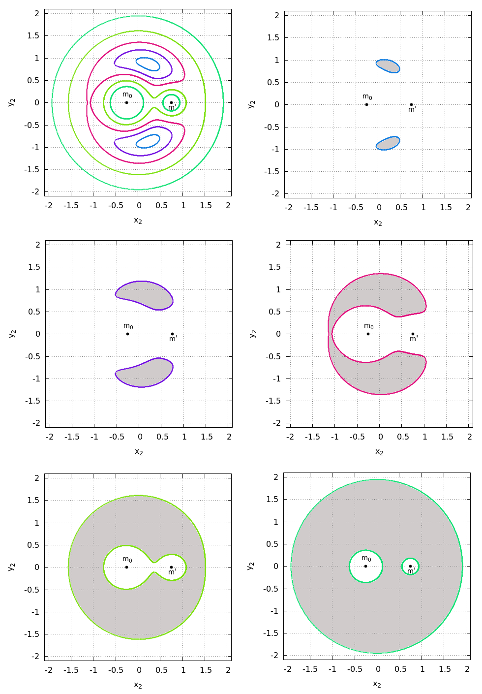
Despite the lack of preservation of the angular momentum and total energy that renders impossible to compute an exact solution, the Jacobi integral still allows to discriminate regions where the motion is allowed from those where it is not. From we obtain the so-called zero velocity surfaces, i.e. a set of surfaces that bound the motion in the system. If we consider only the intersection of these surfaces with the plane (), we reduce the surfaces to zero velocity curves. For the definition of the latter, we just assume that in the expression of (1.108), thus
| (1.111) |
where , are the coordinates of the test particle. Since the velocity of the test particle must be real, the motion is limited to those regions where (see Eq. 1.107), and the zero velocity curves trace the analytic border of these regions. In Fig. 1.8, we provide a few examples of the computation of these delimiting borders. We consider a value of the mass parameter and different Jacobi integral values. From top to bottom, left to right, the values for the Jacobi constant are (blue), (purple), (pink), (yellow-green), (green). The shadowed areas correspond to the forbidden regions. The plot in the upper left panel shows together all five curves. The positions of the masses and are represented by black dots, according to Eq. (1.94).
Even if the Jacobi integral looks not so restrictive, there are several conclusions that can be raised from its analysis. For instance, in the last panel of Fig 1.8, we present the zero velocity curve for the particular case of . If the test particle is located in the region enclosing , it is impossible for the particle to escape from the system or to orbit around , since this would require crossing the forbidden region. For a different (smaller) value of , in the fifth panel, the permitted area surrounds both primary masses, so the test particle may be transfered from an orbit enclosing to one enclosing , but it is not allowed to escape from their common domain. Also, a test particle with initial conditions outside the external zero velocity curve cannot orbit one of the two masses individually. On the other hand, as the value of the Jacobi integral decreases, the forbidden regions become smaller (first panel, Fig. 1.8), and for values smaller than , they disappear.
The Lagrangian equilibrium points are those points in the synodic frame where the centrifugal and gravitational forces are balanced (see §3.5 of [92]). Their computation can be done directly from the equations of motion (1.101), (1.102) and (1.103). As in [13], we adapt the expression of the potential , in order to facilitate the computation of the derivatives involved. Considering the definitions of the distances and in (1.95) and (1.96), we have
| (1.112) |
therefore the potential can be expressed as
| (1.113) |
This version of lacks an expression of the direct dependence on and , substituted by and . Thus, the partial derivatives of are computed as follows
| (1.114) | ||||
For the stationary condition, we consider that both the acceleration and velocity are null (). So, by Eqs. (1.101), (1.102), (1.103), we have that the points for which Eqs. (1.114) are equal to zero are those corresponding to the equilibrium positions. Replacing the partial derivatives with the corresponding formulæ derived from (1.113), we find the equations for the equilibrium positions
| (1.115) | ||||
| (1.116) | ||||
If we set , Eq. (1.116) is trivially satisfied. Also, we get , . Substituting to Eq. (1.115) allows to fine the x-coordinate of the collinear Lagrangian points , and (see [13]). These points are unstable and lie all on the line connecting the star with the planet. Of particular importance below is the point , shown in Fig. 1.9. On the other hand, inspecting Eqs. (1.115) and (1.116), we see that corresponds also to a solution. Considering Eqs. (1.95) and (1.96), we obtain
| (1.117) |
that provides two different solutions
| (1.118) |
Since , the positions of or and those of the two main masses and lie at the vertices of two equilateral triangles. The solution (1.118) defines the equilateral equilibrium points and . We note that these points represent equilibria in the synodic rotating frame. Thus, a particle at rest in or has a circular orbit with angular frequency in the inertial system of reference.

An important point regarding the Lagrangian points is the characterization of the motion in the vicinity of the equilibrium position. We compute the associated value of the Jacobi integral for particles at rest in such positions. We find
| (1.119) |
Figure 1.9 shows the zero velocities curves corresponding to for . The first value is very close to that corresponding to a particle at rest in , while the last value is close to that of , . If , the motion in the vicinity of is energetically allowed to take place surrounding the Lagrangian points or only (although it is not energetically restricted to do so). On the other hand, if , the orbits necessarily surround all three points . This distinction raises two different kinds of motion in the neighbourhood of the equilateral points, known as tadpole and horseshoe orbits. Nevertheless, this study of the motion is inconclusive as far as a stability study has not been done.
1.3.3 Linear stability around the and
Let us consider the position of the massless body as a small displacement with respect to the position of (or )
| (1.120) |
where and are the two small displacements and and are given in Eq. (1.118). We now replace Eq. (1.120) in the equations of motion for the test particle (1.101) and (1.102)33 3 Eq. (1.103) is not considered because we focus on planar motions (on the primaries’ orbital plane). The solution for the vertical component of the spatial case is simply an oscillator [92].. The corresponding linearized equations of motion (see Sect. 1.1.5) are
| (1.121) |
where
| (1.122) |
represent the partial derivatives of the potential evaluated at (,). The linearized system can be represented in a matrix form as in Eq. (1.52), by considering
| (1.123) |
where is a square matrix of constant coefficients.
For the particular case of the stability around the equilateral Lagrangian points , we have
| (1.124) |
Hence, the characteristic equation (1.54) in this case reads
| (1.125) |
whose solutions are given by
| (1.126) |
| (1.127) |
We can see that the eigenvalues are strictly imaginary if the condition
| (1.128) |
holds. This implies that the linear stability is guaranteed only for
| (1.129) |
Equation (1.129) is known as the Routh criterion [50]. If we limit ourselves to the cases within the Solar System, all the systems well represented by the R3BP as, for example, the Sun-Jupiter-asteroid or the Earth-Moon-spacecraft systems, accomplish condition (1.129)44 4 The only relevant exception is the system Pluto-Charon-asteroid. This is a case of a binary rather than a hierarchical system.. Thus, the stable motions around the equilateral points provide an interesting and common feature of the dynamics in the Solar System and most probably in other planetary systems as well. Nevertheless, these results are applicable in very small domains, where the linearization of the system is a valid approximation. More general results can be provided only by the use of non-linear stability theorems (Sect. 1.1.5) or by numerical analysis of the orbits.
1.3.4 Numerical examples

From Eq. (1.126) and Eq. (1.127), and assuming that is small, we can obtain
| (1.130) |
where the subscripts and stand for ’fast’ and ’synodic’ respectively. Equation (1.130) corresponds to the lowest order (in ) approximation of the eigenvalues. If we consider that the solution is a linear combination of the modes of and , then the motion results
| (1.131) |
and
| (1.132) |
where the coefficients and come from the expression of the corresponding matrix in Eq. (1.53). Equations (1.131) and (1.132) clearly show the oscillatory nature of the motion, when a small displacement , is considered with respect to the position of the equilibrium point. The frequencies of the oscillations are given by and . The two oscillations have very different timescales (1.130). On one hand, is approximately equal to , i.e. it gives an oscillation of period similar to that of the motion of the primary around the star. On the other hand, is proportional to the square root of the small parameter , which is a small parameter itself. Thus, the motion of the test particle can be decomposed in two different contributions: the slow motion, associated to the motion of an guiding center around the position of equilibrium, with long period and known as the synodic libration, and the fast one, attributed to the short period motion of the particle around the guiding center. The two motions correspond to two different ellipses, whose dimensions are associated to the amplitudes and . Figure 1.10 represents schematically the decomposition given by Eqs. (1.131) and (1.132). The small ellipse in the figure corresponds to the fast motion of the particle, while the big ellipse gives the libration of the epicenter around the Lagrangian point. The elongated ellipse describing the motion of the guiding center is roughly determined by the size of a corresponding zero velocity curve. The rate of the semiaxes if approximately (§3.10 of [92]). For the ellipse that describes the motion of the particle around the guiding center, it can be proved that (§3.8 of [92]).

Figure 1.11 shows two examples of numerical integrations for these orbits. We integrate the equations of motion for the test particle in the synodic system of reference (1.98), for a time equal to several revolutions of the primaries, for two different orbits. The initial conditions considered for the first orbit (pink) are . The initial conditions for the second orbit (green), , are chosen so that the second orbit presents a larger displacement with respect to the equilibrium point with respect to the first one. In both cases, the chosen mass parameter corresponds to . In the figure, the decomposition of the motion in the synodic and epicyclic oscillation is clear: these yield the elongated tadpole-shaped deformed ellipse enclosing and the smaller ellipse around the guiding center. For larger displacements (as for the green orbit), the synodic libration of the guiding center turns to be larger as well. In this case, the angular excursion of the test particle with respect to the position of is more than . Additionally, the curves show that the angular extension of the orbits is not symmetric, extending (in the case of the green orbit) up to twice the distance in the direction of than in the direction towards the primary. This characteristic pattern of the curves around the equilateral points gives the name of tadpole to this kind of orbits.
It is possible to check, by means of numerical integrations, what happens for orbits more and more displaced with respect to the Lagrangian points, and to compare with the tadpole cases considered before.

Figure 1.12 represents the orbits of two additional numerical integrations performed for the same system as in Fig. 1.11, with . The initial conditions used for these plots are highly displaced with respect to : we consider for the blue orbit and for the green orbit. As expected, due to the shape of the zero velocity curves (Fig. 1.8), the orbits now enclose both lagrangian points and , describing a horseshoe shape. The second orbit (green, right panel Fig. 1.12) is chosen in order to reduce the fast oscillations around the epicenter, rendering possible to visualize the libration: the orbit resembles an extremely elongated deformed ellipse. For comparison purposes, we expose in the figure the curve corresponding to the first (pink) orbit of Fig. 1.11. We recall here that for a fixed value of the Jacobi integral, an orbit cannot get closer to the Lagrangian points than the corresponding zero-velocity curve. Thus, although not entirely limiting the motion, the zero-velocity curve can rule the inner boundary and thus, effectively, the shape of the orbit.
1.4 The Trojan problem
The description given so far is only accurate if the heliocentric orbit of the primary (e.g. planet) is circular (since the solutions come from such an approximation), and the motion of the test particle is planar and takes place in the vicinity of the equilateral Lagrangian point. The study of the motion under a non-circular approximation needs a more elaborate analysis and it is deferred to later in this work. Let us note here that in real systems of astronomical interest, the motion of the planet can itself be quite complicated, since in general it can be influenced by other planets. We can thus consider a hierarchy of problems, passing from the circular to the elliptic R3BP, the secularly evolving R3BP with one or more additional disturbing bodies, etc. As we will see, in all these problems, for small perturbations, we can still have tadpole-like motions of the massless body, whose analytical description becomes, however, more and more cumbersome. In the sequel we will refer to the general problem of the study of such tadpole motions as the Trojan problem.
The study of the Trojan problem has a long history in the literature. Various authors have emphasized different aspects of the problem, and have introduced a variety of sets of variables and/or techniques in order to facilitate its analytical or numerical study. We now briefly refer to some (non-exhaustive) literature on the subject.
Focusing on the case of the CR3BP, early works ([117], [21], [22], [46], [47], etc.) emphasized two main aspects of the problem, namely i) the form and nature of the periodic orbits, and ii) the development of approximative series solutions representing the orbits in the tadpole domain.
In the CR3BP, it can be shown that a set of periodic Lyapunov orbits (in the synodic frame) bifurcates from the equilibrium points L4 or L5 ([101], [102], [103], [26], [46], [49]). For these are short period orbits, i.e. orbits forming a small circle around the equilibrium points. This circle represents the epicyclic motion along a Keplerian ellipse as viewed in the synodic frame. The motion takes place with a period . On the other hand, for we have the family of long period orbits, i.e. elongated orbits surrounding again L4 or L5 but with period , i.e. much longer than the short one. In the limit of the linearized solutions of Eqs. (1.131) and (1.132), these periodic orbits correspond to the cases where the terms associated to one of the two frequencies vanish. Physically, this means that the short period family consists of orbits with a null guiding center oscillation, while the long period family consists of orbits with a null epicyclic oscillation. When nonlinear terms are also taken into account in the orbital equations of motion, each of the two families can be constructed by a formal elimination, in analytical series solutions, of the latters’ dependence on either the short or the long (synodic) frequencies [22]. Then, one finds that the periods turn to have a dependence on the Jacobi constant and on the mass parameter [48].
Furthermore, there exist more complicated periodic orbits which form ’bridges’ connecting the long with the short period family ([104], [105], [25]). These more complicated periodic orbits correspond to a commensurability between the fast and the synodic frequency. Namely, if , with integer, there exist periodic orbits forming epicyclic oscillations (e.g. loops, like in Fig. 1.11) while they accomplish one full synodic libration. Varying and , such orbits can be traced down to their bifurcation either from a short period or a long period orbit. Also, the phase space structure is influenced by such orbits, which give rise to domains of so-called ’secondary resonances’ ([46], [104]). The study of these resonances is a principal part of the present thesis (see Chapters 3-5).
Along a different line of approach, several authors presented series expansions for the Trojan orbits in general, i.e., not restricted to the periodic cases. Among the first of such attempts, in [21] quasiperiodic orbital solutions in terms of the two main frequencies and were calculated via trigonometric expansions called ‘d’Alembert series’. The presence of secondary resonances affects also these series, as it gives rise to so-called critical terms, i.e., terms depending on a resonant combination of the angles. In normal form constructions, such terms cannot be averaged (i.e. eliminated by the usual canonical transformations as in subsection 1.1.4). Thus, their presence prevents the splitting of the normal form Hamiltonian in a ‘short period’ and a ‘secular’ (i.e. long period) part and requires a special treatment (e.g. [46], see also Chapter 5 below). On the other hand, in the Trojan problem it can be shown that their effect on the slow (secular) motions is rather limited [93].
Let us mention, finally, that the use of averaging techniques allows to simplify the study of the synodic librations by finding a simplified form of the equation of motion for the so-called critical argument , with , the mean longitude of the test particle and the planet, respectively. The libration of around the () value () can be represented by a Newton-equation using a so-called ‘ponderomotive potential’ [94]. Studying the properties of this function, it is possible, for example, to express the center of the libration as a function of the eccentricity, inclination and longitude of the perihelion of the Trojan body. It is found that the position of the center in some cases may be shifted considerably from the position of the Lagrangian points and [94]. Some new analytical expressions for this shift are given in Chapter 3.
Whereas the CR3BP may be a good first model for developing the theory of Trojan orbits, it clearly does not suffice to represent more realistic problems. As a natural extension, there exist several approximations to the analytical solution of the Trojan problem in the framework of the Elliptic Restricted 3-Body problem (ER3BP). This generalization brings new interesting features to the formulation. While most works on the CR3BP consider two time scales (associated to and ), in the ER3BP three times scales are necessary [34], associated to the fast, synodic and secular frequency. From the physical point of view, these three scales are associated to the epicyclic oscillation (fast, ), the libration around the libration center (synodic, ) and the slow precession of the perihelion of the orbit of the Trojan body (secular, ) [35].
Starting from an analytic solution up to second order in the mass parameter in [34], for the planar case, and in [35], for the spatial case, it is possible to derive explicit formulæ for the variation of the libration angle and of the major semiaxis of the Trojan body as series in a paramater , called the proper libration [37]. This corresponds to the amplitude of the synodic librations which represents an approximate constant of motion. We find:
| (1.133) | ||||
| (1.134) |
Regarding the secular motions, in [36] approximate formulæ were given for the time evolution of the components of the so-called eccentricity vector ,
| (1.135) | |||
with
Again and are positive constants of integration, is the major semi-axis of the primary , its eccentricity and most of the expressions are up to order . Equations (1.133) and (1.134) represent the shift in the position of the libration center with respect to [37]. This result yields a further correction, depending on , for the shift of the center with the orbital elements , and found in [94].
On the other hand, according to Eqs. (1.135), in the elliptic problem () the center of the eccentricity vector appears displaced from the origin, due to the (constant) terms depending on and in the expressions of and . A generalization of Eqs. (1.135) for the spatial ER3BP is presented in [38]. The two slow time scales ( and ) affecting different orbital elements appear clearly depicted in the equations above.

In Fig. 1.13 we present some examples of numerical computations of Eqs. (1.135). We fix the value of the libration amplitude and the primary’s eccentricity . Ten different values of are used for the generation of orbits. The minimum value corresponds to the innermost and the maximum to the outermost orbit. In the left panel, the initial conditions are apparently divided in two regions according to whether the angle oscillates between two extremes or takes all possible values in the interval . The limit curve labeled corresponds to the orbit with . That curve is not associated with any real structure of separatrix. The motions for are called paradoxal in [8]. They imply a regime of libration of , which is a consequence of the non-zero eccentricity of the primary’s orbit, since, for , could only circulate. However, this libration regime does not stem from a separatrix structure, as made clear from the right panel of Fig. 1.13, which shows that the paradoxal and non paradoxal motions are topologically equivalent in the eccentricity vector plane.
While the previous solutions apply to the cases where the motion of the primary is a given fixed ellipse, it is known that the influence of additional bodies perturbs the motion of . The so-called Laplace-Lagrange theory ([12], for an extension up to second order in the masses, see [70]) allows the remove the short-term behaviors in the motion of the planets under the assumption of no mean motion resonances. In this case, the eccentricity vector of the primary () can be expressed as a secularly varying quantity, depending periodically on the secular frequencies associated with the other bodies. By replacing this behavior in the solutions of Eqs. (1.135), we can recover the effect of a secularly precessing primary on the orbital elements of the Trojan [39]. Since, in general, the time-scale of the secular precession of the primary is long compared with the synodic timescale of the libration of the Trojan, this effect is not evident for just one libration period. Nevertheless, for the long-term behavior, the precessing primary induces widenings of the structures depicted in Fig. 1.13, by shifting the position of the center of libration on a very long periodic timescale. An orbit which for a big value of is paradoxal (librating), may become non-paradoxal (circulating) for a different (smaller) . Thus, the variations of may induce a change of regime in the long-term evolution of the orbit, passing from perihelion circulation to libration or vice versa [39], [110] (but see also Chapter 4). In addition, the introduction of additional frequencies in the problem may induce an increment of chaos and affect the borders of the domain of stability [110]. Also, if the Trojan particle is not limited to the plane of and , additional effects are produced by the variations in the Trojan body’s inclination [39].
Finally, under the assumption that the additional bodies are not in mean motion resonance with the Trojan (nor the primary), it is possible to average the equations of motion with respect to the fast angles and obtain a general secular theory approximation for the Trojan motion, where only the long-term behavior is highlighted [86], [87].
The above approaches emphasize the study of individual orbits under various configurations of the disturbing bodies (planets, etc.). However, a different line of research deals with the characterization of the long-term stability of the orbits.
The stability of the motion around the center of libration in the CR3BP was studies in several contexts. Besides linear stability [50], which holds approximately only in an extremely small domain in which the linear approximation is valid, the theorems of non-linear stability (see Sect. 1.1.5) have been also used. Regarding, in particular, the periodic orbits associated to and , invariant tori delimiting the motion around them were constructed in the planar [23] and in the spatial [78] approximation. In addition, for a small set of the Trojan asteroids of the Sun-Jupiter system, it has become possible to approximate their orbits by KAM tori, by use of the Kolmogorov normalization [45].
In a different approach, it can be shown theoretically that, in the framework of the CR3BP, the necessary conditions for applying Nekhoroshev’s theorem in the vicinity of the Lagrangian points hold true for every value of , except three isolated values [9]. As introduced in Sec. 1.1.5, the Nekhoroshev theorem does not provide a division of the phase-space in systems of 2 d.o.f, as the KAM theorem does. However, by fixing the Nekhoroshev time in Eq. (1.56) to an appropriately large time, it is possible to determine the size of a domain around the elliptic fixed point within which the orbits remain practically stable up to the time . This concept is known as effective stability [51], and it allows to prove that there exist (small) regions that are Nekhoroshev-stable around the equilateral points during the expected lifetime of the Solar System in the case of Jupiter’s Trojan asteroids, for the CR3BP ([51], [16], [52], [113], [31], [30]) and in the elliptic approximation ([74]). Further generalizations in a Hamiltonian formalism for an elliptic problem different to that of Jupiter’s asteroids are presented in [33].
So far, we summarized some important results provided by analytical developments of the theory of Trojan motion. Although these provide some explicit approaches to the solutions, they are also quite limited by the simplifications of the models considered. More complex and realistic approaches can be studied by means of numerical integrations. Several of these studies are devoted in particular to the understading of the dynamics of the Trojan asteroids in the Solar System, where basic models such as the CR3BP or the ER3BP do not reproduce accurately enough the true dynamics [44].
The first Trojan body ever observed was the asteroid Achilles, coorbital to Jupiter. Nowadays, in the libration regions of Jupiter there are more than 6000 bodies observed and classified. When modern computers allowed to produce large simulations, it was possible to test the long-term stability numerically, including also the direct effect of additional bodies. It was found that the orbits in the Trojan swarm are not indefinitely stable. As a consequence, the swarm suffers a slow process of ’erosion’ in the borders of the Trojan domain, due to the gravitational effect of the giant planets [69]. About 5%-20% of the observed Trojans are not stable in a scale of 4 Gyrs [116]. The main responsable factor for the chaos induced in the Trojan swarm are resonances. In [106] and [107], the families of the most prominent resonances that take place within the Trojan libration domain are identified. The secular interaction with Saturn (which is slightly out of the 5:2 MMR with Jupiter) turns to produce remarkable effects. In particular, the family of the resonances involving the secular frequency of the Trojan and the difference (where and are the mean motions of Jupiter and Saturn respectively) seems to be the main cause of the ’erosion’ of the Trojan swarm detected in [69].
One of the benefits from the study of this set of asteroids is that the large number of identified objects makes statistical studies feasible. The theoretical analysis of the Trojan motion evidences the existence of approximate integrals of motion in the secular solutions, called proper elements. They are: the amplitude of libration (directly related to the constant discussed above), the proper eccentricy and the proper inclination . In more general models (or longer numerical integrations) these quantities are not exactly constant, but secularly changing, thus they remain quasi-invariant for long periods of time [10],[112].
The fast variation of the proper elements is an indication of highly chaotic orbits. However, there exist several cases of stable chaos in orbits for which the Lyapunov times are small (i.e., the Lyapunov exponents are big), but the variation of proper elements is negligible [85]. Figure 1.14 presents an updated computation of syntethic proper elements [85], done by using the semianalytical model of [7], where the different timescales presented in the case of Jupiter’s Trojan asteroids are exploited by means of adiabatic invariance theory.

It is conjectured that groups of asteroids with very similar proper elements could have been generated by the collisional disruption of a bigger body. The numerical computation of proper elements for a big number of asteroids allows their classification into families [85].
For several years, it was thought that the population of Jupiter’s Trojan domain was sustained by the accretion, captures or collisions in situ [118], although the mechanisms were proven not to justify properly the features of the real Trojans [79]. In fact, numerical simulations of planetary migration have shown that a slow change of the position in the orbits of Jupiter and Saturn, resulting in their crossing the mutual 2:1 MMR, (the so-called Nice model) could lead to a complete depletion of Jupiter’s Trojan domain [82], [80], even if without such crossing the migration itself could be harmless [56], [108]. On the other hand, although the crossing of one or more planetary MMR induces a considerable amount of chaos, it also makes possible the chaotic capture of new Trojans [89]. A reformulated version of this mechanism is presented in [97], where the hypothesis of a scattering between Jupiter and a lost icy planet is introduced (the so-called Jumping Jupiter model). The latter models are so far the only able to reproduce the inclinations of the observed Trojan asteroids and, perhaps, the asymmetry presented in the number of the objects observed in the two domains.
Regarding the remaining planets in the Solar System, nowadays it is known that there exist coorbital companions at least for Mars, Neptune, Uranus and the Earth. Neptune presents the second most populated Trojan domain, after Jupiter, with 12 components, with characteristically high inclinations. The stability in the equilateral libration regions is proven to be high, thus Neptune may have kept about the 50% of its Trojan population after the migration process [96],[76]. The high inclination values give hints that the main contributions to the population may be due to captures of bodies rather than collisions [75]. As happens with Jupiter and Saturn, the crossing of the MMR with Uranus depletes the region but may trigger also the capture mechanism [75]. Studies of the stability were performed by numerical N-body simulations for Mars ([83], [115]) and Uranus ([96], [28]). In the case of the Earth, its only observed Trojan companion has been shown to be only temporarly trapped in the libration region [18].
Regarding Saturn, numerical simulations show that the secular interaction with Jupiter suffices for destabilizing the coorbital domain [61], [96], thus Trojan companions are not expected for Saturn. Nevertheless, in Saturn’s system of moons, there are two cases of coorbital resonances: Telesto and Calipso are librating Tethys’s and domains respectively, and Helene and Polydeuces are librating Dione’s and .
With the advent of extrasolar planets observations, the spectrum of architechtures for planetary systems has been widened considerably. Extrasolar systems reveal planetary configurations that differ from that of the Solar System, and therefore, the question of the existence of Trojan bodies in these new enviroments takes importance. Such an existence would require examining at least two different topics: i. the possibility of formation or capture of a Trojan body, and ii. the long-term stability of such bodies in the 1:1 libration region of the coorbital planet. Regarding the first point, some authors have studied the possibility of formation of a Trojan planet within the libration region by accretion of material. In general, accretion can produce only small size planets [8]. If two initial coorbital bodies compete for the accretion of material, the process is dominated by the body more massive initially [20]. On the other hand, if the process is individualized, i.e. the dominant body already finished its accretion process, bigger Trojan bodies are feasible to obtain [77].
Regarding the stability of the extrasolar Trojans, some parametric studies were performed for different planetary masses and configurations [95], in some cases applied to observed systems [111]. Of different coorbital configurations, the libration around the equilateral points seems to be the most stable [114]. The architecture of the extrasolar system is determinant for the stability of a Trojan coorbital: the stability regions are more dependent on the physical and orbital parameters of the primary, as well as their correlation with additional planets, than on the mass of the Trojan body itself [41].
Despite the predictions based on the simulations about formation and stability, there are no observed extrasolar Trojan bodies so far. Although different authors examinated the possibility that the libration of Trojan bodies may generate characteristic signatures in the observations of planetary transits [59] or stellar radial velocities [95], these signatures may be highly misinterpreted by the usual techniques of identification [42], [27], [54]. Nevertheless, tests on new methods specifically designed for the detection of Trojan bodies have given promising results [67], [68]55 5 For more extense reviews on the Trojan problem, see [40] or [109]..
1.5 Summary
From what was exposed in the previous introductory paragraphs, it becomes clear that the dynamical richness of the Trojan problem represents a challenge for its theoretical study based on some form of perturbation theory. In this thesis, we attempt to address this problem by: i) introducing a novel Hamiltonian formulation and ii) proposing novel normal form schemes able to deal with the particular characteristics of the Trojan motion. Such characteristics are the existence of differentiated temporal scales, the asymmetry of the motion with respect to the libration center, and the singular behavior of the equations of motion at large libration amplitudes.
In Chapter 2, we define a new normal form algorithm implemented to the CR3BP. We use modified Delaunay-Poincaré variables which make possible a separation of the fast from the synodic d.o.f. The only real singularity of the Trojan problem is due to close encounters of the Trojan body with the primary . Such a singularity implies that expansions in the critical argument around the value converge only in the domain (and similarly for ). In Chapter 2 we propose a novel normal form construction which avoids completely expansions in the variable . Applying the Lie series technique for averaging the fast degree of freedom (independent of ) renders possible to construct a normal form unaffected by the functional form of all series quantities on . We provide a complete description of the expansions and of the proposed normalizing scheme. We finally test the normal form obtained by this method by means of numerical experiments.
In Chapter 3 we revisit the main features of the ER3BP. Starting again from a representation in terms of modified Delaunay variables, we propose a sequence of canonical transformations leading to a Hamiltonian decomposition in the fast, synodic and secular d.o.f. From the latter, we introduce a model called the ’basic Hamiltonian’ . This corresponds to the part of the Hamiltonian independent of the secular angle. The three d.o.f. interact through different resonances, that we classify according to the frequency relation which they involve. These resonances may destabilize the orbits, inducing escapes. By means of numerical experiments, we depict the resonance web in the ER3BP in terms of stability maps and phase portraits. We finally show that there exists a correlation between escapes, sticky regions of the phase space and resonant dynamics.
Chapter 4 is devoted to the study of the dynamics under . The basic Hamiltonian is a model representing the short period and synodic components of the Trojan motion. Averaging over the fast angle, the turns to be an integrable Hamiltonian, yet depending on the value of . Thus, it allows to formally define action-angle variables for the synodic d.o.f., even when . In addition, by means of a trivial reinterpretation of the canonical transformation, it can be proven that the functions derived from the ER3BP and the one derived from a more complex model involving more disturbing planets, called the Restricted Multi-Planet Problem (RMPP), are formally the same. Based on this formal equivalence, we study numerically some properties of the model , using for convenience the ER3BP as a complete model allowing numerical comparisons, although the results are expected to hold in the RMPP as well. In addition, we introduce a method for locating the position of the secondary resonances based on the use of the normalized . We show that the combination of the normalizing scheme of Chapter 2 (adapted here to the elliptic approximation) and the representation by the is efficient enough so as to allow to locate the so-called transverse resonances involving also very slow secular frequencies.
Chapter 5 deals in detail with the problem of Trojan secondary resonances. We formulate yet one more novel expansion allowing to predict the size and the location of secondary resonances in the phase space. This is possible by implementing a resonant normal form on the basic Hamiltonian model . To this end, we face the issue of expansions in the critical angle (Chapter 2). This is addressed by introducing a new expansion called asymmetric. The latter stems from exploting the natural asymmetry of the Trojan orbits in their angular excursion away from or . We make a comparison of the asymmetric and symmetric expansions performed around the Lagrangian points. The symmetric expansion proves to be inadequate for a correct representation of the problem, inducing spurious dynamics in particular cases of resonances. The use of the asymmetric expansion partially remedies this issue.
Chapter 6 summarizes the conclusions of the present thesis, and gives some perspectives on possible extensions for future work.
Chapter 2 Novel normalizing scheme of extended convergence
2.1 Motivation
As already emphasized in the previous chapter, the Trojan motion in the ER3BP has three components, with well separated temporal scales: a fast (epicyclic) motion with frequency of order , a synodic motion with frequency of order and a secular motion with frequency of order . Due to the decoupling of the secular d.o.f., in the CR3BP the motion can be expressed in terms of the fast and the synodic frequencies only, as in Sect. 1.3.4.
As customary in Celestial Mechanics, the most basic form of Hamiltonian normalization stems from averaging the Hamiltonian over the fast angles. Independently of the formalism used, what remains after such averaging gives the synodic motion around the libration center. The use of a suitable set of variables is necessary for performing the averaging. A good choice for this purpose are Delaunay variables (see Sect. 2.2 below).
Regarding the above, we point out a crucial remark. The Hamiltonian of the CR3BP has a real singularity corresponding to close encounters of the massless body with the primary . This singularity takes place at , . The key remark is that any polynomial series expansion of the equations of motion (or the Hamiltonian) with respect to around a fixed value is convergent in a disk of radius equal to the distance between the fixed point and the singularity. In the literature, it has been common to consider such polynomial expansions around the position of equilibrium (). Due to the asymmetry of the librations (Sect. 1.4), it is easy to see that the above limited convergence affects severely the representation of the orbits mainly in the opposite direction to the primary (see Fig. 2.1).

We will now present a Hamiltonian scheme allowing to average the Hamiltonian over short period terms without making expansions affected by the singular behavior of the Hamiltonian at . In the framework of the CR3BP, the so found averaged Hamiltonian is an integrable system of one d.o.f. able to describe the synodic librations in the whole domain of allowed Trojan motion. We then test the degree of approximation of our analytical method against numerical experiments.
2.2 Delaunay-Poincaré expansion for the pCR3BP
We start from the Hamiltonian of the planar R3BP in heliocentric cartesian coordinates, given in Eq. (1.90). By the system of units defined, we have . Thus,
| (2.1) | ||||
where , is the heliocentric position vector for the planet, for the Trojan and . This decomposition of (including a term in the disturbing function) allows to define Delaunay variables independent of the mass parameter [14]. The heliocentric vectors in polar coordinates are
| (2.2) |
and (considering the circular approximation for the pR3BP)
| (2.3) |
We can re-express the terms of the disturbing function as
| (2.4) | ||||
| (2.5) | ||||
where (see Fig. 2.2). Replacing Eqs. (2.4) and (2.5) in Eq. (2.1), we find
| (2.6) |
with defined in Eq. (1.93) and . The gravitational potential defining the disturbing function depends only on the relative configuration between the bodies, thus the Hamiltonian is independent of the orientation of the inertial system where the coordinates are defined.
At this point, we introduce the first canonical transformation to Delaunay-like variables, as
| (2.7) | ||||||
where , , , , are the major semiaxis, eccentricity, mean anomaly, longitude of the perihelion and mean longitude of the Trojan body. The Keplerian part of the Hamiltonian (2.7) (see Eq. 1.60) in terms of Delaunay variables reads
| (2.8) |
Due to the splitting performed in Eq. (2.1), it is possible to define the actions of the Delaunay set independently of (unlike in Eqs. 1.81).
The disturbing function in (2.1) contains the quantities
For the expansion of , we have
| (2.9) |
Thus,
| (2.10) |
where are trigonometric (finite) polynomials of degree in the mean anomaly. The construction of this expansion is based on the expansions for the true anomaly in terms of the mean anomaly (see, e.g., §2.5 of [92])
| (2.11) | ||||
where
| (2.12) |
are the Bessel functions of first kind and their derivatives. Substituting with (2.11)–(2.12) in (2.10) we obtain the trigonometric polynomials . Up to order :
For the expansion of , from Eq. (2.9), we have
| (2.13) |
Replacing Eq. (2.11) into Eq. (2.13), it is possible to compute . Up to order :

For the expansion of , we first expand , considering that (Fig. 2.2). Hence,
| (2.14) | ||||
Replacing all the above expressions in (2.6), and setting , the Hamiltonian is given by
| (2.16) |
The Hamiltonian in Eq. (2.16) is a system of d.o.f., since the action conjugated to does not appear explicitely. In order to produce an autonomous Hamiltonian, we add a dummy action , with no other physical meaning than to complete the set of canonical variables. We define through Hamilton’s equations, , , so the extended Hamiltonian is
| (2.17) |
Equation (2.17) corresponds to a sytem of 3 d.o.f. Nevertheless, it is possible to trivially reduce one of them, by the following remark: all the trigonometric terms in the disturbing function have arguments of the form
| (2.18) |
with , . As a consequence of the invariance of the Hamiltonian to rotation transformations, the coefficients must satisfy the following condition
| (2.19) |
known as the first d’Alembert rule. In the pCR3BP, the variables and do not appear, hence . Also, since , the longitude of the perihelion of the circular orbit of does not appear in the disturbing function (second d’Alembert rule), thus . Hence,
| (2.20) |
If we replace (Eq. (2.7)) in Eq. (2.18) for the pCR3BP, we obtain
| (2.21) | ||||
Thus, as a consequence of the d’Alembert rules, and appear in the Hamiltonian exclusively through the difference . This fact can be checked explicitely, for instance, in the expansions up to order of Eq. (2.15).
We thus introduce a canonical transformation through the generating function of second class (old angles and new actions), defined by
| (2.22) |
that generates the transformation equations
| (2.23) | |||||||
Applying this transformation to (2.16), we obtain
| (2.24) |
where . This form of is independent of , thus remains constant in time. Since a constant term in the Hamiltonian does not induce any effect on the dynamics of the problem, we directly neglect it. We keep the original symbol for those variables that were transformed by the identity transformation.
In order to avoid the fictitious singularity that takes place if (Sect. 1.2.3), we introduce Poincaré-like variables, through the transformation 11 1 We symbolize with the function , of two variables, that maps the value of the arctangent to the corresponding quadrant in the coordinate system with as the abscissa and as the ordinate.:
| (2.25) | ||||||
A similar set of coordinates but dependent on is used in [46]. By the computation of the Poisson bracket, it is straightforward to check that the transformation (2.25) is canonical. In these new variables, the transformed Hamiltonian reads
| (2.26) |
In Delaunay-Poincaré variables, the fast and synodic dynamics are represented by the two independent pairs of canonical coordinates. The first terms of the Keplerian part of Hamiltonian (2.24) read
| (2.27) | ||||
where and are back-transformed according to and . Thus, the frequencies associated to each angle are
| (2.28) |
where we assume that , and are small quantities in the neighborhood of the Lagrangian points. Hence, the normalizing scheme only has to remove the dependence of the Hamiltonian on or, in Poincaré variables, it has to remove any combination of and different from .
We will now show that, by means of canonical transformations based on Lie series, it is possible to introduce a normalizing scheme that removes and on which is not involved. This allows to keep a complicated dependence of the Hamiltonian on , avoinding to introduce expansions in the synodic variables () with convergence problems due to singularities, as mentioned before. We notice that the term that induces this singularity is , which contains the factor
| (2.29) |
Expanding the Hamiltonian in Eq. (2.26) with respect to , and , we obtain the polynomial expression of H, given by
|
|
(2.30) |
where is defined in Eq. (2.29) and the coefficients are rational numbers. The Hamiltonian in Eq. (2.30) is the function that we use for initializing the normalization.
In practice, these expansions are easier to perform if the intermediate step associated to the variables (2.7) is avoided, and we pass directly from the orbital elements , , to Poincaré-like variables. In the Appendix A, we provide explicit formulæ for these expansions, including the construction of the terms with dependence on .
2.3 Normalization scheme
The elimination of the fast angle , in our variables, implies to obtain a Hamiltonian that depends on and only through powers of (Eq. 2.25). Such terms are said to be in normal form. Each step of the algorithm, based on Lie series, eliminates terms depending on of certain order in two small parameters: and a given combination of , and .
Let us first introduce the following definition:
Definition 2.3.1
A generic function belongs to the class , if its expansion is of the type:
where are real coefficients.
Definition 2.3.1 classifies the terms appearing in the algorithm according to their dependence on the powers and ruling the iteration step. The relation between the exponents of the variables is a consequence of the application of Poisson brackets of during the algorithm (see Proposition 2.3.3 below) and make the formal algorithm consistent. Let and be two integer counters, in the intervals and respectively, with the fixed maximum orders of normalization. Let us assume that the Hamiltonian expansion at the -th step is such that
|
|
(2.31) |
where , , , , and . In words, contains terms in normal form up to order in , and order in , , with , , the exponents of , and respectively. For greater orders, the dependence on and is polynomial but arbitrary.
The -th normalization step requires to compute
| (2.32) |
with the operator , in Eq. (1.33) and the generating function to be determined. With this aim, we introduce the following propositions:
Proposition 2.3.2
If and , then there exists a generating function and a normal form term satisfying the homological equation
| (2.33) |
Proposition 2.3.3
Let and be two generic functions such that and , then
We just sketch the procedure to follow so as to determine a solution of (2.33). First, we replace the fast coordinates with the complex conjugate canonical variables , such that and . Since the kernel of the homological equation does not depend on slow coordinates , the Poisson bracket does not affect them. Thus, we expand the homological equation (2.33) in Taylor series with respect to , using as fixed parameters. We solve term-by-term the equation (2.33) in the unknown coefficients and such that
|
|
and
|
|
Finally, we express the expansions above by replacing with , and we obtain the final solutions in the form and . Regarding Prop. 2.3.3, its proof just requires long but basically trivial computations, thus it is omitted.
By construction, the generating function satisfying Prop. 2.3.2, generates a Hamiltonian , through the transformation (2.32), that is in normal form up to order , i.e.,
|
|
(2.34) |
where , ,
,
,
and . The additional terms
induced by the transformation of Eq. 2.3.3
correspond to higher orders in and , and they are normalized in
subsequent steps of the algorithm.22
2
It is straightforward to
prove that the above normalizing scheme corresponds to an algorithm of the
kind described in Sect. 1.1.4 with the following
book-keeping rule:
Rule 2.3.4
To every monomial of the type
there corresponds a book-keeping parameter of type ,
given by
where is the maximum order of normalization for .
The Hamiltonian in (2.30) is in a suitable form for starting the normalization step (). Thus, the whole algorithm consists of the subsequent determination of the Hamiltonians
| (2.35) |
up to the maximum orders . Nevertheless, since this process is finite, the last computed Hamiltonian
| (2.36) |
which is in normal form up to orders and , differs from the original Hamiltonian by a remainder term . The best choice for the truncation orders and are those values that make this remainder minimum. In practice, we encounter computational limitations enforcing to fix a priori the values of . In the sequel, we check that the truncation order is not very inaccurate by numerical tests showing how well the normal form reproduces the dynamics of the original Hamiltonian .
2.4 Numerical studies on the normal form
2.4.1 Semi-analytical integration scheme
Let us denote by the set of canonical coordinates introduced at the –th normalization step. Let be
| (2.37) |
By the ’Exchange theorem’ (Eq. 1.34), we have that
| (2.38) |
Thus, the whole normalization procedure is described by the total canonical transformation
| (2.39) |
connecting the normalized variables , with the non normalized variables .
With the total canonical transformation, we provide the following semi-analytical integration scheme
|
|
(2.40) |
where denotes the flow induced by a generic Hamiltonian on the canonical coordinates, for an interval of time equal to . In words, we estimate the time evolution of the non-normalized system by the study of the normalized system, provided we perform the transformations accordingly between initial and final conditions. This integration scheme provides just an approximate solution, which is more accurate as smaller the remainder part is with respect to .
We note here that is integrable and its flow is easy to compute. To this end, we introduce the temporary action–angle variables , such that and . is a constant of motion for the normal form . Thus, we compute and at any time by the quadrature method, with as a fixed parameter. Regarding , we compute the integral corresponding to the differential equation . Finally, the values of and are obtained from and . For practical purposes, the application of the classical quadrature method can be replaced by any numerical integrator. Due to the available computational resources, in the numerical experiments that follow, the maximum truncation powers are , , for and respectively.
2.4.2 Numerical surfaces of section and semi-analytical level curves


The comparison between the normalized Hamiltonian and the complete pCR3BP is done by means of numerical computations. Since the former is a system of 1 d.o.f. and the latter is a system of 2 d.o.f., the illustration of the pCR3BP dynamics is made through phase portraits, i.e. so-called Poincaré surfaces of section.
This method consists of retaining the points of the orbits that intersects a particular surface, defined by a section condition. A suitable (transverse to the flow) surface allows to distinguish the dynamics of the problem, roughly discriminating between periodic, quasi-periodic and chaotic orbits (see Fig. 2.3). In action-angle variables, the quasi-periodic orbits lie on invariant tori (Sec. 1.1.3). Back transforming to the original variables, the portrait under the full Hamiltonian resembles a deformed version of the portrait under the normalized Hamiltonian, with the addition of possible chaotic orbits.

In Fig. 2.4 we show an example of a pericenter surface of section for the pCR3BP, defined by the condition
| (2.41) |
We obtain the phase portraits as follows. We fix the value of the mass parameter and compute the value of the energy in (2.26) for the point (, ). We define initial conditions on the surface of section (), by varying and choosing such that is equal for all the initial conditions of the set. We translate the initial conditions to cartesian variables () and we integrate Eqs. (1.3.2) with a Runge-Kutta - order integrator, along 500 periods of the primaries, with time-step equal to . During this integration we collect the points contained in the surface of section and finally the output data is again translated to Delaunay variables and plotted. Since the surface of section condition corresponds to exactly one period of the fast angle , the portrait represents the dynamics of the synodic d.o.f., as in the normal form . Thus, the orbits computed by the normal form and the phase portraits are possible to compare.
The example presented in Fig. 2.4, for , gives an estimation of how the libration regime of the pCR3BP looks like. One of its most characteristic features is the large, asymmetric variations in . For this value of , it is possible to recover also some horseshoe orbits, librating around the two equilateral points. A successful normal form must be able to recover these properties of the Trojan motion. Hence, in the experiments that follow, we test whether the normal form: i. efficiently reproduces the large variations of the angle , in particular for orbits close to the border of stability, and ii. distinguishes between tadpole and horseshoe orbits, in the cases where stable orbits exist in both domains.
The first test is a graphical comparison between the orbits provided for each Hamiltonian. The initial conditions used are fictitious, but each set is derived from the catalogued position of a real Trojan body, called the generating body. A whole portrait corresponds to a value of the Jacobi constant equal to the one of the generating body. We show below examples for two generating bodies, namely 2010 TK7, Trojan asteroid of the Sun-Earth system and the asteroid 1872 Helenos of the Sun-Jupiter system.
From a catalogue, we obtain the coordinates (rotated to the plane of primaries) of each generating body for a certain epoch, that we transform to . This initial condition provides the Jacobi constant for the body. The set of 10 initial conditions are generated by , , a variable value for and such that (isoenergetic orbits). These orbits are numerically integrated for a short time, up to accomplishing . The final values used for the integrations, gathered in , lie on the surface of section .
We first compute the numerical surfaces of section of the pCR3BP for the initial conditions in in the same way as in Fig. 2.4. Passing now to the normal form, the invariant curves of the numerical surface of section correspond to level curves of . To compute the latter, we first translate the initial conditions of to normalized variables, applying the inverse total canonical transformation . From , we derive Hamilton’s equations for and ,
| (2.42) |
which provide the flow induced by the normal form. We numerically integrate the normalized initial conditions, up to collecting about 2000 points, and keeping the relative energy error smaller than . The resulting orbits lie on the level curves of the integrable normal form corresponding to the values , given by , of each initial condition of . We complement for every point the values and (equivalent to ). Let us note here that the use of numerically integrated orbits in order to obtain the level curves of the normal form is only done for numerical convenience. In principle, these curves are possible to obtain just from the algebraic solution of the level curves equation . Also, the condition in the normalized coordinates does not correspond exactly to the surface of section in the original variables. However, since is by definition a near-to-identity canonical transformation, we assume that the two conditions do not differ too much and avoid computing the exact section which involves quite cumbersome formulæ. Finally, via , we back-transform all the points of a level curve to the original variables.
Examples and results

We choose two systems with very different values of the mass parameter for a better contrast in the results. The first case corresponds to the Sun-Earth system, with . The generating body is the Earth’s Trojan asteroid 2010 TK7. We obtain its coordinates from Jet Propulsion Laboratories JPL Ephemerides Service33 3 http://ssd.jpl.nasa.gov/?ephemerides, at epoch 2456987.5 JD (2014-Nov-26), that in Poincaré variables read , , and . The second case corresponds to the Sun-Jupiter system, with . The generating body is the Trojan asteroid 1872 Helenos, that librates around . The initial conditions for Helenos are taken from Bowell Catalogue44 4 http://www.naic.edu/nolan/astorb.html, at 2452600.5 JD (2002-Oct-22), that in Poincaré variables read , , and .
Figure 2.5 shows the comparison between the surface of section and the level curves computed for the Sun-Earth system (left panel), and Sun-Jupiter system (right panel). In both cases, the points of the surface of section are shown in pink, while the level curves of the normal form are shown in green. In the case of the Sun-Earth system, the agreement between the two representations is very accurate. The averaged Hamiltonian reproduces accurately the large variations of and distinguishes between tadpole and horseshoe orbits. On the other hand, in the case of the Sun-Jupiter system, due to a larger value of , the system is substantially more chaotic, a fact that the normal form cannot reproduce. Nevertheless, the normal form is able to simulate well tadpole orbits provided by the pCR3BP, as far as such orbits are not trapped in a secondary resonance between the fast frequency and the synodic libration frequency (see Sect. 1.4 and 3.3).
2.4.3 Computation of quasi-actions
As an additional test, we analyze some orbits that were not accurately represented by normal forms in the past literature. In [45], the stability of some observed Jupiter’s Trojan asteroids was studied by constructing KAM tori solutions for these asteroids. Of the 34 initial conditions used in [45], the Kolmogorov normalization algorithm did not work properly in seven cases. Here, we revisit the latter 7 initial conditions (1868 Thersites, 1872 Helenos, 2146 Stentor, 2207 Antenor, 2363 Cebriones, 2674 Pandarus and 2759 Idomeneus). These orbits either lie very close to the border of stability or show an anomalous behavior with respect to the expected tadpole orbit, so they represent an interesting test for our new normal form.
The normal form contains two different actions or integrals of motion. One, obtained by construction, is . The other, not explicitly obtained, is due to the fact that the normal form is a 1 d.o.f. system. This second constant of motion is associated with the area enclosed by the level curves of and , and it should be reproduced by the normal form. For the comparison of the areas in the two Hamiltonian, we produce the corresponding level curve as well as the numerical invariant curve for each initial condition. From the curves, we extract the maximum and minimum values for and , and we obtain the position of the center for the curve provided by the averaged Hamiltonian

| (2.43) |
and the center for the numerical orbit
| (2.44) |
Fig. 2.6 shows the curves, the extreme values and the centers obtained in one of these cases. The discrepancy between the two centers, which shows how much displacement there is between the orbits, is computed by
| (2.45) |
We re-express the points of each curve with respect to its center, by introducing the quantities and . We obtain the distance to the center and the angle with respect to the horizontal line (). Re-ordering the points from small to large values of , we compute the triangular area generated by two consecutive points and the center. The sum along all the triangles represents the contained area within each curve, for the complete system and for the averaged Hamiltonian flow55 5 An alternative analytical way to estimate the area is given by Green’s formula. For a further comparison, we compute also the relative difference between the areas , and the displacement of the centers with respect to the position of the corresponding equilateral Lagrangian point (, for and for ).
| Asteroid | |||||
|---|---|---|---|---|---|
| 1868 | |||||
| 1872 | |||||
| 2146 | |||||
| 2207 | |||||
| 2674 | |||||
| 2759 |
For six of the seven cases mentioned above, we obtain averaged orbits that reflect the behavior of the numerical integrations. In Table 2.1 we report the results of the computations described before. The averaged areas clearly match their associated numerical areas, with a relative error smaller than 2%, except in one case (asteroid 2146 Stentor), for which the error is about 13%. This may be due to the large displacement that its center has with respect to the equilateral point. For the rest of the asteroids, the orbits on the surface of section and the corresponding analytical level curves agree. On the other hand, in Table 1 we do not present data for the highly inclined () asteroid 2363 Cebriones. For this asteroid, our normal form failed to provide an accurate orbit, using the initial conditions provided in [45]. However, we find that the numerical orbit generated by 2363 Cebriones presents a very peculiar angular excursion (in ) with respect to the Lagrangian point. Furthermore, the failure of the normal form could be due to an imprecise evaluation of the initial condition, caused by a non-consistent rotation to the plane of the primaries in the original work [45].
Chapter 3 The elliptic Trojan problem
In the previous chapter we provided a new normalizing scheme that allows to study the synodic libration of the Trojan orbits, in the framework of the pCR3BP. Notwithstanding the degree of approximation of this study, it is known that several aspects of the Trojan orbits are ruled by the fact that the orbit of the primary is not circular but elliptic.
In the present chapter, we revisit the main features of the planar ER3BP, by means of a convenient Hamiltonian formalism where the three d.o.f. appear well differentiated. This construction allows to explicitely obtain the main frequencies of the motion, which interact through different kinds of resonances.
By means of numerical experiments, we depict the resonance web in the ER3BP in terms of stability maps and phase portraits. Our results from a statistical study of escapes show that there exists a correlation between escapes, sticky regions of the phase space and resonant dynamics.
3.1 Expansion in terms of modified-Delaunay variables
We start the construction of the Hamiltonian function from (1.90) in Sect. 1.3.1:
| (3.1) | ||||
where , and are the heliocentric position vectors for the planet and for the massless body, and is given in (2.2). However, since we now consider the elliptic approximation, there holds that
| (3.2) |
where is the distance to the star and , the polar angle measured from the -axis, accomplishes , where and are the true anomaly and the longitude of the pericenter of the primary. With no other bodies perturbing the motion of the planet, its ellipse is fixed in the space and is constant in time. We expand each term of the disturbing function as in the circular case,
| (3.3) |
| (3.4) |
where in both expressions . Substituting Eqs. (2.2), (3.2), (3.3) and (3.4) in Eq. (3.1), we obtain
| (3.5) |
where now also is a function depending on the time.
We introduce, as first step, modified Delaunay variables , independent of the mass parameter and given by
| (3.6) | |||||
where , , and are the mean longitude, the longitude of the pericenter, major semiaxis and eccentricity of the orbit of the Trojan body. The primed symbols correspond to the orbital elements of the planet. Considering , (see Sec. 1.2.2) and
| (3.7) |
(Eq. 3.6), the expansions for the true anomaly are given by
| (3.8) | ||||
where , are Bessel functions of the first kind and their derivatives, given in Eq. (2.12). Similarly, we obtain and . According to the units of measure defined in Sect. 1.3.2, , while and (through ) act as parameters. Thus, the expansions for the true anomaly of the primary are
| (3.9) | |||
| (3.10) |
On the other hand, by the definition of the actions in Eq. (3.6), we have
| (3.11) |
whereby, after replacing Eqs. (3.8), we obtain
| (3.12) |
and
| (3.13) |
Considering Eq. (3.12), the series for in terms of () is obtained as in Chapter 2.
Gathering the previous expressions, we construct the disturbing function in terms of modified Delaunay variables. The expansions up to the second order in the eccentricities are presented in Appendix B. The Hamiltonian (3.1) in the new variables reads
| (3.17) |
where . As shown below, in computing proper elements there turns to be crucial to remove the dependence of the Hamiltonian on time by introducing a ‘dummy’ action variable conjugate to , namely
| (3.18) |
The present expression of the Hamiltonian corresponds to an autonomous system of 3 d.o.f, while (3.17) is a d.o.f. system.
For the study of the Trojan dynamics, we define two new angles, namely and . The angle is the resonant angle corresponding to the 1:1 MMR resonance, with value at the Lagrangian point . The angle expresses the relative position of the pericenter of the Trojan body from the pericenter of the planet. We introduce these new angles through a generating function depending on the old angles (, , ) and the new actions (, , ),
| (3.19) |
yielding the following transformation rules
| (3.20) | |||||||
Note that preserving the canonical character of the variables requires some modification of the dummy action variables as well. We keep the old notation for all variables involved in a identity transformation (, , ). The Hamiltonian then reads:
| (3.21) |
This expression can be recast under the form:
| (3.22) |
where
| (3.23) |
and
with
The action is an integral of motion under the Hamiltonian flow of . Thus, the Hamiltonian represents a system of two d.o.f. We call position of the forced equilibrium the solution of the system of equations
| (3.24) |
We find
| (3.25) |
From (3.25), we can deduce that the equilibrium point is not given by a fixed point in the synodic frame of reference, as it happens in the circular case. In particular, since , a Trojan body with elements deduced from (3.25) describes a fixed ellipse of eccentricity in the inertial frame. Thus, the body describes a short-period epicyclic loop around in the synodic frame.
3.2 The motion around the forced equilibrium and the three temporal scales
We now introduce local action-angle variables around the point of forced equilibrium. The purpose is to characterize the motion by two approximate constants, one of which appears as an action variable () on the plane around the value , while the other appears as an action variable () on the plane around the value . To this end, we introduce the ‘shift of center’ canonical transformation given by:
| (3.26) |
where
where is defined negative so as to keep the canonical structure with respect to . Re-organising terms, the Hamiltonian (3.21) takes the form:
| (3.27) |
where contains terms depending on the angles and only through the difference , and contains terms dependent on non-zero powers of . This splitting suggests to perform one more canonical transformation, through which the part of the Hamiltonian corresponding to can be formally reduced to a system of 2 d.o.f.:
| (3.28) |
yielding
| (3.29) | |||||||
The subscripts ‘f’ and ‘p’ stand for ‘fast’ and ‘proper’ respectively, for reasons we explain later. As before, we keep the old notation for the variables transforming by the identities , and . However, it turns to be convenient to retain the new notation for the action . The Hamiltonian (3.27) in the new canonical variables reads
| (3.30) |
Collecting terms linear in , we find:
| (3.31) |
We identify and as the short-period and secular frequencies, respectively, of the Trojan body. Comparing Eq. (3.31) with Eq. (1.130), we see that the fast (short-period) frequency recovers the same value as in the CRTBP. Therefore, the set of variables constructed in (3.28) allows to separate the three time-scales of the 3 d.o.f. The main contributions to the frequencies come from the Keplerian part and , because provides terms of at least first order in , where both the mass parameter and the eccentricity are small parameters.
The above decomposition of the Hamiltonian allows to consider various ‘levels’ of perturbation. We call basic model the one of Hamiltonian
| (3.32) |
The total Hamiltonian takes the form , where
| (3.33) |
contains terms of at least order . Since is ignorable, is an integral of the motion for the flow induced by the Hamiltonian (3.32). The physical importance of can be understood as follows: the action variable measures the radial distance from the point of forced equilibrium in the plane , in which the forced equilibrium is located at the origin. In a first approximation, the quasi-integral of the proper eccentricity can be defined as
| (3.34) |

However, the above definition neglects the fact that is subject to fast variations due to its dependence on . In fact, by Hamilton’s equations we readily find that . The time variation of is associated to a fast frequency . In fact, by their definition we can see that the variables describe epicyclic oscillations of the Trojan body, i.e. accomplishes one cycle every time when the Trojan body passes through a local pericenter. The time variations of become particularly important when one of the following two conditions holds: i) , or ii) the orbit of the Trojan body is subject to a low-order resonance. On the other hand, remains an exact integral of the Hamiltonian (3.32) even in the cases (i) or (ii). We thus adopt the following definition of the proper eccentricity:
| (3.35) |
In the Hamiltonian (3.32), the integral (or ) becomes a label of a system of two degrees of freedom corresponding to the canonical pairs and . Since the function contains terms of at least first order in , under the full Hamiltonian (3.30). This implies that (or ) remains a good quasi-integral for not very high values of the primary’s eccentricity. On the other hand, a more accurate () quasi-integral can be computed by a first order adiabatic theory [11]. Figure 3.1 summarizes the physical meaning of the various action-angle variables . We emphasize that in numerical computations one always stays with the original (Cartesian) co-ordinates of the various bodies. Then, translation of the results to action-angle variables and vice-versa is straightforward, passing first to Delaunay elements, and then using the transformations (3.19), (3.26), and (3.28). The functions and , with an error , are given in the Appendix C.
A second averaging over the fast angle yields the Hamiltonian
| (3.36) |
with
In Chapter 4, we compute a more precise averaged model by means of a normalizing scheme similar to the one of Chapter 2, but implemented in the ER3BP. For the moment, we just focus on some basic properties of . The Hamiltonian represents a system of one degree of freedom, all three quantities serving now as parameters, i.e. constants of motion under the dynamics of . The Hamiltonian describes the synodic (guiding-center) motions of the Trojan body, with the additional point that, since it depends on , it does not correspond to the averaged (over fast angles) Hamiltonian of the circular RTBP. From a physical point of view, this expresses the possibility to find an integrable approximation to synodic motions even when .
The equilibrium point given by
corresponds to a short-period periodic orbit of the Hamiltonian around the forced equilibrium point. We define the action variable
| (3.37) |
where the integration is over a closed invariant curve around and ‘s’ stands for ‘synodic’ (see Fig. 3.1). The angular variable , conjugate to , evolves in time according to the synodic frequency given by (see Eq. 3.44)
| (3.38) |
Some manipulation of Eq. (3.36) allows to find a first order approximation to the values of the frequencies and . We deduce the shift in position, with respect to L4, of the fixed point of , corresponding to the short-period orbit around L4 [94]. The shift is given by , where is the solution of . We find:
| (3.39) |
where the error is of order 4 in the eccentricities , .
We introduce the following canonical transformation, to analyze the motion around the position of the periodic orbit given by
| (3.40) |
where, in terms of the new actions, we have , yielding
| (3.41) | |||||||
In the new variables, the angles and contain a trigonometric dependence on terms oscillating with the synodic frequency, due to . Since , we have , . However, since in Eq. (3.36) does not explicitely depend on these angles, the conjugated actions and remain integrals of motion. As in the previous cases, we keep the notation for those variables that were transformed by the identity (, , ). Taylor-expanding , around up to terms of order , we find (up to terms of first order in and second order in the eccentricities):
| (3.42) | ||||
where . Since is , up to terms linear in the part
| (3.43) |
defines a harmonic oscillator for the synodic degree of freedom. The corresponding synodic frequency is
| (3.44) |
On the other hand, the secular frequency is given by . Assuming a harmonic solution , and averaging over the synodic period , we find
| (3.45) |
completing the estimation of the frequencies. We remark here that Eq. (3.45) applies for orbits in the neighborhood of the short period orbit and it is in agreement with the results of Érdi [37], [38].
3.3 Secondary resonances in the ER3BP
The Trojan domain describes itself a resonant regime, defined by the 1:1 commensurability of the mean motions of the Trojan body and the planet. In addition, within this domain, we can find secondary resonances of the form
| (3.46) |
with integers. The most important of all these resonances are those involving low order conmensurabilities between and . These resonances exist in the complete spectrum of possible problems, from the pCR3BP () up to the complete Restricted Multi-Planet Problem RMPP (see Chapter 4). They are of the form
| (3.47) |
with . We briefly refer to a resonance of the form (3.47) as the ’:’ resonance, and to higher order resonances as the : resonances. For and in the range , is in the range . In the frequency space , the relations (3.47) represent planes normal to the plane which intersect each other along the –axis. In the same space, all other resonances with intersect transversally one or more planes of the main resonances. We refer to such resonances as ‘transverse’. In the numerical examples below, we use the notation , for the integers of the resonant condition (3.46). In Sect. 3.6, by means of numerical experiments, we show the effect of these resonances in the rate of chaotic diffusion.
Under the Hamiltonian flow of , a : resonant periodic orbit forms fixed points on a surface of section , for . Around the fixed points of a stable resonant periodic orbit there are formed islands of stability (see Fig. 3.1), surrounded by separatrix-like thin chaotic layers passing through the unstable fixed points. This kind of resonance bifurcates from the short-period orbit at (equivalent to , see Eq. 3.40) provided that
| (3.48) |
where we can identify the fast and synodic frequencies. Such orbits appear in pairs, one stable and one unstable, and it is known that they form ’bridges’ connecting the short period family with the long period family [25] (cf. discussion in Sect. 1.4). Under the full Hamiltonian dynamics of , the bifurcation generates a 2D-torus, which is the product of the above orbit times a circle on the plane with frequency .
Beyond the bifurcation point, as increases, the fixed points move outwards, i.e., at larger distances from the central fixed point , while the resonant islands of stability grow in size. The growth is faster for lower-order resonant periodic orbits (i.e. for smaller ). This growth, however, stops when the islands of stability enter in the main chaotic sea around the tadpole domain of stability. Numerically computed examples of this behavior are given in Sec. 3.4.1.
3.4 Numerical experiments
In this section we present a parametric survey of the resonant structures appearing in the space of proper elements (,). We focus in the main secondary resonances, of the form (3.47) and its associated multiplets. As we show in the numerical experiments, this kind of resonance dominates the phase space, affecting in particular the domain of stable orbits. This study is based on two parts: we first present a survey of phase portraits, illustrating the phase space structure in the circular case. In this case, the phase portraits can be visualized by a 2D surface of section, while in the elliptic case the corresponding section is 4-dimensional (this issue is discussed in detail in Chapter 4). On the other hand, based on the phase portraits of the circular case we construct sets of initial conditions which can be used in the elliptic problem as well. With these initial conditions, we construct an atlas of stability maps applying to the ER3BP, computed by means of a suitable chaotic indicator.
3.4.1 Parametric study of surfaces of section
As introduced in Sect. 2.4.2, Poincaré surfaces of section supply a good visualization of the dynamics of 2D orbits. Of all possible surfaces, it turns practical to consider apsidal sections in which the orbits pass through consecutive local pericentric or apocentric positions. Here we adopt the pericenter crossing condition, and , where is the radial velocity in the heliocentric frame. Note that this is the same condition as for the phase portraits of Chapter 2, (Fig. 2.4).
The pericentric surface of section is two-dimensional if , and four-dimensional if . In the circular case, in the Hamiltonian (3.30) becomes equal to zero by identity. The exact invariance of is equivalent to the exact invariance of the Jacobi constant in the barycentric rotating frame. In practice, it is more convenient to construct surfaces of section of constant values of rather than . Yet, we label these surfaces of section using a corresponding value of . This correspondance is established in the following way: to a given value of corresponds a short-period orbit crossing the chosen surface at a fixed point with coordinate (Eq. 3.39), with . Noticing that, for the angles and coincide ( can be defined without loss of generality equal to zero), i.e. , the remaining initial conditions of the fixed point are given by
| (3.49) |
The condition on is the pericenter crossing condition. Setting the Delaunay action as , and the angle , with at , one then has all four values of the Delaunay variables , whereby cartesian position and velocity vectors can be computed. This allows to compute the Jacobi constant corresponding to the short-period orbit of given . We refer to the whole surface of section with as the section corresponding to a ‘given value of ’ (referred to as ’the proper eccentricity’), although, for fixed , actually changes somewhat as we move on the section away from the point (see Chapter 4). Now, for any other point on the surface of section, the pericentric condition yields , while (and hence the precise value of ) can be computed by solving numerically the Jacobi-constant equation . We produce surface of section plots taking 35 equispaced initial pericentric conditions along a fixed line of the form , up to , and solving always the equation . The inclination is determined according to a rule explained below. For each initial condition, we integrate the orbits and collect 1000 successive points on the surface of section, plotted in the plane .

We repeat this process for different values of , from to , with an interval of , and with . This range of values contains the resonances of the form 1:n, with . Higher order resonances of the form :, : or :, etc., are distinguishable by visual inspection.
In Figure 3.2, we show some examples of this computation. The plots for (upper row) and (lower row) correspond to the pericentric Poincaré surfaces of section in two cases where the resonances : and :, respectively, are conspicuous in phase space. We note that one of the fixed points of the stable periodic orbit corresponding to the 1:6 resonance lies on the horizontal line . This is so for all even resonances (i.e. : with even). On the other hand, for odd resonances (: with odd) all stable fixed points lie on lines of the form with . In our stability maps, we use the slopes given in Table 3.1. The line of initial conditions in each case crosses the border of the stability islands close to its mots widely separated points, a fact allowing a better visualization of the resonance.
| Resonance | slope | |
|---|---|---|
| : | 0.0014 | 0.04 |
| : | 0.0021 | 0.025 |
| : | 0.0031 | 0.015 |
| : | 0.0056 | 0.03 |
A resonant periodic orbit 1:n bifurcates from the central short-period orbit at pairs of values satisfying Eq. (3.48). As shown in Fig. 3.2, for fixed , the resonant orbits move outwards as increases, while their corresponding island chains grow in size. The three panels in each row of Fig. 3.2 correspond to three different values of (see caption), in increasing value from left to right. For small values of , the stability islands in both cases are surrounded by invariant tori. The stability domain around extends from to , for . Some small higher order resonances are visible at the border of the stability domain. However, as increases, the resonant islands grow in size, while most of the external invariant tori are destroyed. For a critical value of , the last KAM torus surrounding the resonant island chain is destroyed. We find that this value satisfies in all studied cases. For , the resonant islands are surrounded by the outer chaotic sea, which penetrates the stability domain closer and closer to the center. Thus, for the right boundary of the stability domain shrinks to or less.
Similar phenomena appear if is kept fixed while varying . As increases beyond the bifurcation value, the stability islands of the resonance move outwards and increase in size. Reaching a certain critical value of , the last invariant torus at the border of stability surrounding the islands is destroyed. This mechanism also shrinks the stability region, although by abrupt steps. On the other hand, different values of give rise to different resonances. Thus, the size of the domain of stability undergoes abrupt variations connected to the bifurcations of new resonances (see [41] for a quantitative study of this effect in the case as well as Fig. 3.13 below).
3.4.2 FLI stability maps
As mentioned before, if , the pericentric surface of section becomes 4-dimensional and, due to projection effects on the plane , a detailed visualization of the resonant structures becomes unclear (see discussion in Sec. 3.5 and Chapter 4). Nevertheless, a convenient visualization is possible in the space of the actions . In practice, we demonstrate all results in a space of proper elements (libration angle) and (proper eccentricity), which are in one to one relation with the action variables . The quantity is defined as follows: for given , we first determine via Eq. (3.39). Then, we consider all invariant curves around the equilbrium point of the one degree of freedom Hamiltonian in Eq. (3.36), as well as a line of initial conditions , where, in all examples below, for even resonances, or as indicated in the Table 3.1 for odd resonances. We call the point where the invariant curve corresponding to the action value intersects the above line of initial conditions. Finally, we set . Using the harmonic oscillator approximation of Eq. (3.43), the action can be approximated as , where is given by Eq. (3.44), while is the oscillator energy found by substituting the initial conditions to Eq. (3.43). Then, up to quadratic terms in , one has
| (3.50) |
Note that for odd resonances, is not equal to the half-width of the oscillation of the variable along the invariant curve of corresponding to the action variable , which is used as a standard definition of the proper libration angle. Instead, locating the point where the ellipse defined by intersects the axis , we find
| (3.51) |
In the numerical simulations, after fixing and , we chose a grid of initial conditions in the square , , setting also and with , , . This completely specifies all Delaunay variables for one orbit, and hence its initial cartesian position and velocity vectors. We also set the value of the dummy action in the Hamiltonian (3.18). Finally, we express (3.18) in the original Cartesian form
| (3.52) |
and keep track of the constancy of the numerical value of the energy as a probe of the accuracy of numerical integrations.

Stability maps are computed over the above grid of initial conditions by means of color-scaled plots of the value of a suitable chaotic indicator. Here we employ the Fast Lyapunov Indicator (FLI, see [43]) given by
where is the variational (deviation) vector computed by solving the variational equations of motion along with the orbital equations of motion and denotes the norm. For computing FLIs we implement a th-th order Runge-Kutta method, with a timestep equal to of the period of the primary ( in our units). We stop integrating orbits that have clearly reached escape so as to avoid numerical overflows. The escapes are identified by a sudden jump of the energy error to levels beyond , while for non-escaping orbits the energy error at the maximum time of integration periods is less than . Also, we stop integrating the variational equations of orbits reaching FLI values larger than .
Figure 3.3 shows an example of computed stability maps for and three values of , namely , , and . In each plot, the value of is given in a color scale for all grid initial conditions in the plane of proper elements . The color scale was set in the range . Regular orbits correspond to darker colors (black) representing low values of , while the most chaotic orbits correspond to light colors (yellow). Orbits with are shown also in yellow.
A more detailed resonance identification is made by means of Frequency Analysis [66]. The most conspicuous resonances are explicitly indicated in all three plots. For (top left panel), the resonance : dominates the stability map. Besides, several resonances of the type produce strips penetrating the stability domain. In agreement with what was shown in the surface of section plots of Fig. 3.2, the width of the : resonance increases, initially, as increases from zero up to a value . Also, the chaotic separatrix-like layers around the resonance remain thin. However, for the resonance is detached from the main stability domain. Then, its corresponding islands of stability are embedded in a chaotic sea corresponding to orbits with a fast escape. For still larger (around 0.1) the central periodic orbit becomes unstable and the corresponding islands disappear. In general, this, as well as all higher order resonances, move outwards (towards higher values of ) as increases. Thus, all resonant strips have a small positive slope in Fig. 3.3.
On the other hand, increasing the value of causes new transverse resonances to appear. For (top right panel), resonances of the form , or , with and up to are distinguishable. We note that in general the angle formed between the transverse resonances () and the secondary resonances of the circular problem () is small (of order ), where and are the respective secular and synodic frequencies. This small transversality implies that the intersection point of most mutually transverse resonances lies in the chaotic zone, i.e. far from the domain of stability. In particular, the transverse resonances with have no intersection with the main resonance : inside the stability domain. In fact, these transverse resonances penetrate the domain of stability in isolated, single-resonance strips, along which the orbits undergo weakly chaotic diffusion that bears many features of Arnold diffusion. On the other hand, the resonances that are beyond the border of the inner stability domain form multiplets, in which the chaotic diffusion has features of modulational diffusion. This gives a mechanism of efficient escape for chaotic orbits (see Section 3.6).
For still higher values of (Fig. 3.3, down panel for ), new transverse resonances appear. In fact, as increases all transverse resonances move in the direction from top left to bottom right, until reaching large values of , after which they enter into the main chaotic sea surrounding the domain of stability. Then, they become less significant.


Figures 3.4 to 3.11 show the atlas of FLI
maps for differents cases of , and for the mass parameters
, , , , , ,
and . These are representative of the multiplets
formed around the resonances 1:12, 1:11, 1:10, 1:9, 1:8, 1:7, 1:6 and
1:5, respectively. In each plot, the values for are ,
, , , and , from top to bottom and left
to right. Inspecting these plots, we emphasize some features.
i) The size of the non-resonant domain does not change much with
variations of . In fact, in all these plots we observe
that, despite the fact that, as evolves, new transversal
resonances appear, the non-resonant domain keeps its limits nearly
constant (at about in Fig 3.4, in Fig
3.5, in Fig 3.6,
in Fig 3.7, in Fig 3.8, in
Fig 3.9, in Fig 3.10 and in
Fig 3.11). On the other hand, the resonant domain, which
for low (but non-zero) values of is filled with small
transverse resonances, gradually shrinks within the chaotic sea, and
for values of around , it completely
disappears. This gives a natural limit for the values of
to consider, since no important resonances survive for .
ii) Around a main resonance, we identify new emerging transverse
resonances, of the kind , with a small integer. Since
they involve a commensurability with , they are not present for
, but for greater values they become evident, especially
some isolated ones which penetrate inside the non-resonant region. As
increases, the whole structure moves outwards (towards
increasing values of ) but their upper limit also moves
downwards (towards smaller values of ). For bigger values of
, the main resonances 1:n generally disappear or they are
small, leaving space for transverse resonances to dominate in action
space.
iii) In Figures 3.5, 3.9, 3.10 and 3.11, we can see traces, appearing as thin darker lines in the chaotic domain (right part of the plot), of the stable invariant manifolds emanating from lower-dimensional invariant objects around , such as the short-period planar Lyapunov orbits in the case , or their associated 2D-tori, for [6]. Figure 3.12 shows an example of comparison of the structures found in the FLI maps with the exact computation of the stable invariant manifolds of the Lyapunov orbit around in the case , , corresponding to panel A of Fig. 3.11. The left panel shows the same structures in greater detail, plotting in pink all points for which the FLI is in the limit . These limits exclude all points corresponding to regular orbits, as well as all escaping orbits, for which the FLI evaluation quickly saturates to a high value . On the other hand, for the middle panel, we consider the interval of Jacobi constant values , where and represent the minimum and maximum value of the Jacobi constant encountered in the whole 400400 grid of initial conditions of the FLI map of Fig. 3.11A. Splitting this interval in 400 values of , for each value we compute numerically the corresponding horizontal Lyapunov orbit around and its stable manifold and we collect all the points in which the latter intersects the section of the FLI map (given by the pericentric condition as well as ). Numerically, we introduce some tolerence in the section determination, in order to collect a sufficiently large number of points necessary for visualization of the results. Plotting in the same co-ordinates as for the FLI map the collected points for all 400 stable invariant manifolds corresponding to the 400 different values of C yields the middle plot of Fig. 3.12. The relative loss of sharpness in the picture of the manifolds is due to the numerical tolerance used in their section’s determination. Despite this effect, we see clearly that the structures formed by the invariant manifolds follow in parallel those indicated by the corresponding FLI map. The possibility to use the FLI (with a small number of iterations), in order to visualize invariant manifolds was pointed out in [58]. Here, this effect can be considered as a manifestation of the so-called ‘Sprinkler’ algorithm (see [64] for a review). Namely, in a system of fast escapes, plotting the initial conditions of the orbits which have relatively large (forward or backward) stickiness times (and, thus, relatively lower FLI values with respect to the escaping orbits) allows to vizualize the (stable or unstable) manifolds of nearby periodic orbits. In fact, the sticky chaotic orbits in the forward sense of time are those trapped within the lobes defined by the stable invariant manifolds (see, for example, figure 19 of [29]). This effect is clearly shown in our example by combining the left and middle panels of Fig. 3.12. The right panel of Fig. 3.12 clearly shows that the points of greater stickiness in the forward sense of time, as revealed by their relatively low (with respect to fast-escaping orbits) FLI values, are located precisely between the limits of the structures indicated by the stable invariant manifolds of the family of the planar Lyapunov orbits around . We note, finally that when , instead of the foliation of all the manifolds of the Lyapunov family, one has to consider the invariant manifolds of a 2D unstable invariant torus around . This computation is numerically hardly tractable. Nevertheless, simple inspection of all panels of Fig. 3.11 clearly shows that the structures found for essentially continue to exist, in a quite similar geometry, in the case as well.


Returning to the discussion of the resonant structure, the overall effect of resonances on the size of the stability domain is resumed in Fig. 3.13. For a set of initial values of , from to , with step , and fixed values for and , the figure shows the FLI map produced by integrations of the set of initial conditions given by , , and varying from to , with step . Darker (black) colors correspond to regular orbits, and light (yellow) colors to chaotic orbits. The main resonances appear as long yellow tongues that contain single or double thin chaotic layers associated to the separatrix (depending on whether the resonance is odd or even). In a similar way, a large number of smaller transverse resonances fills the space between the main ones. By the fact that the tongues are nearly horizontal, we can infer that the presence of particular resonances is highly localized with respect to the value of , e.g. the resonance : is important at , it completely disappears in the chaotic domain at . Also, as increases, a bifurcation of new secondary resonances happens less frequently. Nevertheless, since they are of decreasing order, their width and relative influence increases.
3.5 Modulational diffusion
The resonant periodic orbits arising under the flow of correspond to resonant 2D tube tori under the flow of the full model . Respectively, the resonant fixed points correspond to one-dimensional tori on a surface of section . Projected on the plane , these tori appear as thick curves (see Fig. 3.14 below). In the same projection, the islands of stability and their delimiting separatrix-like chaotic layers are observed to undergo ‘pulsations’, i.e. some periodic shift in the plane modulated at the frequency . This pulsation phenomenon is further described in Chapter 4 (see Sect. 4.2). Such pulsation is induced by the presence (in but not in ) of terms trigonometric in the angle and its multiples.
The modulation of all resonant motions by slow trigonometric terms
results in a long-term chaotic diffusion taking place in the space of
the action variables . In fact, based on the pulsation
width of the separatrices, we encounter the following two diffusion
regimes:
i) Non-overlapping resonances: for small pulsation widths, the
separatrices of one resonance do not enter to the pulsation domain of
the separatrices of nearby resonances. In such cases the rate of the
chaotic diffusion is quite small, and the diffusion becomes
practically undetectable. Also, the geometry of resonances in the
action space is closer to the paradigm of Arnold diffusion [3].
An example of chaotic orbit in such regime is given in
Fig. 3.15 (green orbit).
ii) Partially-overlapping resonances: for large pulsation
widths, the pulsation domains of more than one separatrices of nearby
resonances partially overlap. In this case the rate of chaotic
diffusion increases dramatically. As shown in
Sec. 3.6, the chaotic orbits in the most
prominent chaotic layers exhibit a diffusion timescale of the order or
1Myr. The diffusion leads finally to an escape from the resonant
domain and eventually from the overall tadpole domain. However, there
is also a weakly chaotic population exhibiting long times of
stickiness, with a power-law distribution of the stickiness times
characteristic of long-term correlated chaotic motions
(see [81] p. 843, and references therein). At any rate, in
most cases we find that the overlapping of resonances is not complete,
as is, for example, the case of resonant multiplets for Jupiter’s
Trojan asteroids (see [107]). As a result, the overall
diffusion process in our experiments is closer to the paradigm of modulational diffusion [17]. Finally, there are
regular resonant orbits that never escape the system.
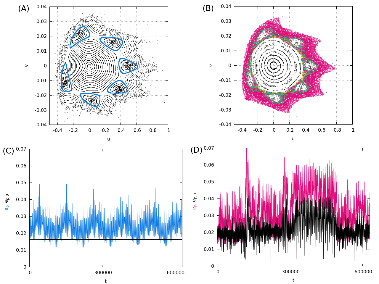
Figure 3.14 gives a typical example of the modulational diffusion regime. The panel (A) shows an apsidal surface of section (see Sec. 3.4.1) which depicts the structure of the phase space in the circular model ( for the dynamics under the Hamiltonian ), when , . For these parameters, the phase portrait is dominated by the islands of the : resonance. The separatrix-like chaotic layers surrounding the resonance are very thin, while the resonant islands are delimited by both inner and outer librational KAM curves. Thus, all orbits inside this resonance cannot communicate with orbits of nearby resonances embedded either in the remaining part of the stability domain or in the chaotic sea surrounding the stability domain. An orbit near the separatrix layer of the : resonance is shown in blue in Fig. 3.14(A). Note that is an exact integral of motion of the flow under , as confirmed by a numerical computation of (Fig. 3.14(C), black curve). On the contrary, the distance from the forced equilibrium which coincides with the osculating value of the eccentricity (Fig. 3.14(C), blue curve) undergoes substantial short-period oscillations (of order ). Thus, as defined via Eq. (4.17) is a much better measure of the proper eccentricity than the usual definition .
Figure 3.14(B), now, shows the projection on the plane of a 4D pericentric surface of section in the elliptic case, when (black points), on which we superpose in colors the points of one chaotic orbit undergoing modulated diffusion. The : resonance is still clearly visible on the projection, giving rise to six islands, one of which intersects the line at values around . Another smaller 6-island chain, intersecting the line at about is also distinguishable. As shown in Fig. 3.3, the latter corresponds to the transverse resonance , whose extent, however is limited and produces no substantial overlapping with other low order resonances. On the other hand, the pulsation of the separatrix of the : resonance does result in a substantial overlapping of this resonance with other outer resonances surrounding the origin. As a result, an orbit started in the separatrix layer of the : resonance later communicates with the separatrix layers of the outer resonances. In the example of Fig. 3.14(B), the orbit with initial conditions indicated in the caption remains confined in the neighborhood of the : resonance up to a time (green points), while at later times (up to ) the same orbit expands to embed several higher order resonances of the form : as well as some transverse resonances of the elliptic problem (pink points). A careful inspection shows that the orbit undergoes several outward and inward motions in the whole domain from the : resonance up to the outer resonances, while the orbit eventually escapes from the system at still larger times (of order ). The various outward or inward transitions are abrupt, and they are marked by corresponding transitions in the value of , which is now only an approximate adiabatic invariant. Such transitions are shown in Fig. 3.14(D) (black curve). Here, an overall comparison with the time evolution of the quantity (pink curve), shows that the definition of via the action variable still yields a useful measure of the proper eccentricity, while presents wild variations even in short timescales. In fact, the time behavior of presents jumps at all outward or inward transitions of the corresponding orbit of Fig. 3.14(B). A further analysis of how the diffusion progresses in the space of action variables is given in the following section.
3.6 Escapes statistics and chaotic diffusion
The co-existence of different types of resonances renders non-trivial the question in which domains of the phase space the chaotic diffusion, due to the interaction of resonances, provides a more efficient transport mechanism for orbits, thus affecting long term stability. As explained in Sec. 3.5, two main regimes of chaotic transport exist. For isolated resonances located inside the boundary of the main stability domain (like the transverse resonances and of Fig. 3.3), the orbits in the stochastic layer have the possibility of slow diffusion that bears features of Arnold diffusion. In any case, we find that the diffusion rate is extremely small, thus it is practically undetectable. On the other hand, for resonances located beyond the boundary of the main stability domain, the diffusion process is best described by the paradigm of modulational diffusion. In particular, the amplitude of pulsation of the separatrix-like chaotic layers at the borders of the resonances is large enough to allow for communication of the resonances, causing the orbits to undergo abrupt jumps from one resonance to another, and eventually to escape.
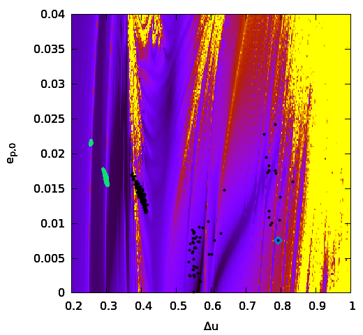
Figure 3.15 provides evidence of the processes mentioned above. Two orbits are shown superposed to the FLI map for , . The initial conditions for both correspond to , but different (, for the orbit in green, and , for the orbit in black). We plot the intersection points of both orbits with the plane when , , with a tolerance and respectively. According to these data, the first orbit resides in the chaotic layer of the resonance , while the second is initially in the chaotic layer of the resonance :. However, the first orbit is restricted to move essentially only along the stochastic layer of the initial resonance, as no resonance overlapping exists with any low-order adjacent resonance. As a result, the orbit’s diffusion is practically unobservable. By contrast, the second orbit suffers a significant change of topology over a timescale of only periods. The orbit visits many other resonances besides the starting one, jumping stochastically between the chaotic layers of the resonances 1:6. , , , and , and possibly other ones of higher order. The proper eccentricity also exhibits abrupt jumps in the interval [,].
The long-term behavior of orbits in the modulational diffusion regime
can be characterized by a statistical study. To this end, we consider
an ensemble of orbits in a rectangle of initial conditions. As an
example, setting, as before, , , we consider a
grid of initial conditions in the interval , , with the remaining initial
conditions defined as for the FLI maps above. The ensembles are
processed at 5 different snapshots, corresponding to the integration
times of , , , and periods. In every
snapshot (of final time ), the orbits are classified in three distinct
groups:
Regular orbits: these are orbits whose value of the
FLI satisfies the condition
| (3.53) |
where is the total number of periods for the integration. Since
for regular orbits the FLI grows linearly with , the threshold of
Eq. (3.53) allows to identify orbits which can be clearly
characterized as regular. These orbits are exempt from further
integration.
Escaping orbits: an orbit is considered as escaping if the orbit
undergoes a sudden jump in the numerical energy error
greater than . This threshold is determined by the
requirement that the jump surpasses by about two orders of magnitude
the worst possible accumulation of round-off energy errors at the end
of the integration time (i.e. after periods). We tested the
cumulative energy error as a function of time for different initial
conditions. Figure 3.16 shows the evolution of for
one example of escaping orbit. The first panel shows the increment of
up to a time . The absolute cumulative error
grows linearly in time at a rate per
period. This rate is characteristic of the orbits in the thin chaotic
layers between the resonances. However, exhibits an abrupt
variation at the moment of escape. Up to
the maximum integration time , the cumulative energy error for
non-escaping orbits is smaller than . Thus, we set a
safe threshold value for escape identifications as .
Transition orbits: we characterize as transition orbits those whose
FLI value violates condition (3.53), but which do not escape during
the integration up to the time . As we will see, part of these orbits
remain at low FLI values up to the end of the integration, yielding
a growth . Thus, the orbits exhibit a regular
behavior up to at least periods. However, a second sub-group is
formed among the transition orbits, containing truly sticky orbits
with positive Lyapunov exponents and FLI values growing asymptotically
linearly with .

With the results at the five different snapshots, a statistical
study of the escaping times is constructed as follows: in the end of every
snapshot,
i) we count the number of orbits belonging to each of the three groups,
ii) we compute the histogram of FLI values (from up to ) for the
transition orbits, and iii) we store the values of and
for both the escaping and the transition orbits. The results of (i) are
summarized in the following table:
| Snapshot | (N. of periods) | Regular | Transition | Escaping |
|---|---|---|---|---|
| 1 | 1220 (%) | 2027 (%) | 353 (%) | |
| 2 | 1263 (%) | 1388 (%) | 949 (%) | |
| 3 | 1296 (%) | 966 (%) | 1338 (%) | |
| 4 | 1299 (%) | 699 (%) | 1602 (%) | |
| 5 | 1309 (%) | 603 (%) | 1688 (%) |

Focusing, now, on the groups of transition and escaping orbits, the upper panels in Fig. 3.17a-e show the distribution of and FLI () values for the transition orbits (green) and the escaping orbits (pink) respectively. In Fig. 3.17a (upper panel), for periods, most of the transition orbits are found to keep a relatively low value of the FLI, , and a cumulative energy error of about . In fact, all the transition orbits with larger become escaping orbits shortly after periods. A second group of transition orbits, however, starts being formed, with FLI larger than or equal to 50. The lower panel shows the distribution of FLI values for all the transition orbits. The left concentration represents regular or very sticky orbits, while the more chaotic orbits are spread over larger values of the FLI, with a small secondary peak formed in the right part of the histogram at . However, as the integration time increases, a ‘stream’ is formed that transports members of the left group towards the right group. As a result, at the last snapshot, ( periods), the right group contains about 30% of the transition orbits and 6% of the total orbits considered. In fact, as visually clear in all upper panels of Fig. 3.17, most escapes occur at intermediate values of the FLI, while the right group is nearly completely detached from the left group of the transition orbits, the latter moving to the right at a speed logarithmic in , i.e. as expected for regular orbits. Finally, the Lyapunov characteristic times of the orbits in the right group are all substantially smaller than , while the orbits remain sticky for times . This behaviour is reminiscent of stable chaos [84].
In addition, we notice that the escaping orbits (pink) seem to form bands of preferential values of the FLI. We do not not fully identify the origin of these bands. Nevertheless, they could be connected to the fact that the escape can occur only via the thin chaotic layers between the resonances, so that the concentration to particular FLI values could reflect the local FLI value for orbits residing for long time within each one of such layers.

Figure 3.18 shows the histogram of escaping times of all the escaping orbits. It becomes evident that in the process of escaping two distinct timescales can be distinguished, corresponding to two peaks of the histogram. The first peak, at about periods, corresponds to fast escapes, while the second, at about periods, corresponds to slow escapes. As shown below, the large majority of fast escaping orbits are with initial conditions within the chaotic sea surrounding the resonances, while slowly escaping orbits are those with initial conditions in the thin chaotic layers delimiting the resonances. In the latter case, we find that beyond a time periods, the distribution of the escape times shows a power-law tail. The straight line in Fig.3.18 represents a power-law fit
| (3.54) |
We note in this respect that power-law statistics of the escape times are a characteristic feature of stickiness and long-term chaotic correlations of chaotic orbits [81].

Finally, Fig. 3.19 shows a comparison between FLI values and the residence (or escape) times for all the orbits of the integrated ensemble. The left panel shows the FLI map for the square of initial conditions . The right panel, now, shows in color scale the residence, or escaping times, for all initial conditions of the ensemble. Yellow colors represent the faster escaping times ( periods), while red the slower (between and periods). In light purple are depicted the orbits that remain in the group of transition orbits up to the end of the integration ( periods), while deep purple represents the orbits belonging to the regular group. The first observation is that the distribution of escaping times reproduces to some extent the main features of the resonant structure found by the stability map. In particular, the chaotic layer of the resonance : appears clearly marked by long escape times (larger than periods). The stickiness is in general enhanced at the borders of all resonances. On the other hand, most of the orbits with or greater, that are qualified as chaotic in the stability map, belong to the population of fast escapes, and we find that most need less than periods to escape. But the most interesting feature is that all the thin chaotic layers around the resonances , , , , , : and , contain orbits that appear not escaping at least up to periods. This, despite the fact that some of these orbits are relatively strongly chaotic, i.e with close to 5. Thus, we can conclude that the stickiness phenomena in the thin chaotic layers formed in the resonant domains of the action space can prolong the stability of hypothetical Trojan bodies up to times comparable to the age of the hosting system.
Chapter 4 The basic Hamiltonian
In the previous chapter, we introduced the so-called ’basic Hamiltonian’ (Eq. 3.32). This model is a 2 d.o.f. system representing the short period and synodic components of the Trojan motion. Its expression comes naturally as a splitting of the complete Hamiltonian in two parts: and a secular term that gathers all the terms depending on the slow secular angle . By averaging the over its fast angle, we can formally define action-angle variables for the synodic degree of freedom. Since the includes the eccentricity of the primary, it allows to find an integrable aproximation to synodic motions even when . On the other hand, it makes a suitable starting point for non-linear stability studies, from a more general point of view than the circular problem (Section 1.1.5).
In the present chapter we start by showing an important property of the : by means of some adjustments in the definitions of variables and canonical transformations considered, it is shown that the Hamiltonian found in the ER3BP is formally identical to a corresponding ’basic model’ found in a more complex model, namely the ’Restricted Multi-Planet Problem’ (RMPP), where we consider the influence of more than one planets on the Trojan body.
We first construct the derived from the RMPP, comparing to the construction of this Hamiltonian in the ER3BP (Chapter 3). Having established the formal correspondence between the two models, we then return to the ER3BP and perform a more detailed analysis of the properties of , using both numerical and analytical approaches. In particular, we numerically investigate up to what extent the decomposition provides a meaningful model. Then, we apply the normalization scheme introduced in Sec. 2.3, which allows to average the Hamiltonian over the fast angle circumventing in the ER3BP as well the convergence problem of large radii. Finally, using this averaged model, we compute analytically the position of the most important secondary resonances and compare the results with those found in the numerical stability maps computed in the previous chapter.
4.1 The Restricted Multi-Planet Problem
The decomposition of the Hamiltonian of the pER3BP that leads to the definition of the (Sect. 3.1 and 3.2) can be generalized in a more representative problem called planar Restricted Multi-Planet Problem (RMPP). This model is based on the pER3BP, but it includes also the secular effects of additional planets on the Trojan body.
The RMPP Hamiltonian is derived as follows. We assume that all the planets are far from mean motion resonances. Their motion is thus described by a set of secular frequencies: for the primary and for additional planets. These frequencies are possible to compute either by a linear (Laplace) theory, by a non-linear analytical extension ([70]), or by purely numerical methods (e.g. frequency analysis, [66]). In any case, we consider that the frequencies , are the frequencies of the leading terms in the quasi-periodic representantion of the oscillations of the planets’ eccentricity vectors. Therefore, we can express their time evolution as
| (4.1) | ||||
where , are the eccentricity and longitude of the pericenter of the primary, and , the corresponding to the th additional planet [90]. Without loss of generality, the constant can be set equal to zero. The positive quantities , , with , and , are referred to below as the amplitudes of oscillation of the planetary eccentricities. Also, we assume that . Then, at least the primary exhibits a constant, on the average, precession of its eccentricity vector, by the frequency , i.e., we can write , , where the functions and depend trigonometrically on the angles , , , while their size is of the order of the amplitudes , . All these latter assumptions are justified if the primary is the most massive planet in the system.
For each secular frequency we introduce now a pair of action-angle variables, i.e. the ‘dummy’ actions and the angles , , . The primary’s elements are given by
| (4.2) |
Then, the Hamiltonian
of the RMPP is found by the following steps:
i. Add to the Hamiltonian of the ER3BP (3.18) the direct terms for planets. The direct term for the -th planet is:
where with equal to the mass of the -th planet, and , , with the heliocentric position vector of the -th planet. Transcribed to elements, depends on . Assuming that the -th planet is far from a mean motion resonance with the primary (and hence with the Trojan body), we compute
By rotational symmetry, depends only on the
difference , and hence, (see Eq. ), only
on the angles , and , . By
d’Alembert rules, this implies that it is also of first or higher
degree in the eccentricity , i.e., it is of first or higher
degree in the amplitudes of oscillation of the planetary
eccentricities.
ii. Consider now the indirect effects of the planets on the Trojan body. Far from mean motion resonances the primary’s major semi-axis remains constant. Then, the indirect effects are accounted for by rendering the parameters in the expression (3.18) time-dependent rather than constants. Replace now Eq. (4.2) in Eq. (3.18) and Taylor-expand, around and , assuming and small quantities. This leads to:
where is of degree one or higher in the quantities ,
and hence, of degree one or higher in the mass parameters ,
.
iii. Adding also terms for all dummy actions , , the final Hamiltonian now reads
| (4.3) |
Two important remarks are in order: i) The function in Eq. (4.3) is formally identical to the function in (3.18), apart from replacing with and with . ii) The functions and , are of first or higher degree in the amplitudes of oscillation of the planetary eccentricity vectors. We note that the case where mean motion resonances between the planets are present necessitates a separate treatment, since then the domain of co-orbital motion can be crossed by resonances of the type of the ‘great inequality’ (see [107]).
From this point on, the procedure for deriving the final Hamiltonian decomposition follows as in Chapter 3. We only give a short sketch, emphasizing the points where differences hold between the two models. Unless explicitely differentiated, the conclusions of Sec. 3.1 and 3.2 hold also here, with similar arguments.
The first canonical transformation introduces the two resonant angles of the planar Trojan problem: and , instead of , for representing the relative position of the pericenter of the Trojan body from the pericenter of the planet (since one has ). Altogether, the transformation reads
| (4.4) |
leading to
| (4.5) | ||||||||||||
where . As in Chapter 3, here also we keep the same notation for variables involved in an identity transformation. After applying the transformation, the Hamiltonian (4.3) takes the following expression
| (4.6) | ||||
The latter Hamiltonian can be split into two terms and . While has the same form as in (3.23) (with the addition of the term ), reads
| (4.7) | ||||
The computation of the forced equilibrium position is done as in Chapter 3,
resulting
| (4.8) |
For the expansion around the forced equilibrium, we consider the shift of center
| (4.9) |
where
We thus construct the synodic action variables in the plane around the value , while the secular action variable () measures the distance from the forced center in the plane .
Re-organising terms, the Hamiltonian (4.6) takes the form:
| (4.10) | ||||
where (i) contains terms depending on the angles , only through the difference , (ii) contains terms dependent only on non-zero powers of and independent of , and (iii) contains terms dependent on and also on non-zero powers of either or the oscillation amplitudes of the planetary eccentricities. In terms of the current variables, we are ready to introduce the basic Hamiltonian as follows
| (4.11) |
The total Hamiltonian takes the form , where
| (4.12) | ||||
Again, the fact that in (4.11) the angles appear only under the combination implies that can be reduced to a system of two degrees of freedom. The reduction is realized by the canonical transformation:
| (4.13) |
yielding
| (4.14) | ||||||
Keeping the old notation for , , but, however, retaining the new notation for the action , the Hamiltonian in the new canonical variables reads
| (4.15) |
We can now see that this form of the Hamiltonian is formally identical in the RMPP and in the ER3BP. From Eq. (4.15), with the substitution and setting , it is straightforward to re-obtain Eq. (3.32). Hence, the basic features induced by apply in the same way with or without additional planets. Furthermore, all extra terms with respect to in the Hamiltonian (3.30) depend on the slow angle , while in the case of the RMPP in (4.10), they depend also on the slow angles , , , whose corresponding frequencies are all secular. Thus, these terms can only slowly modulate the dynamics under . In the case of the ER3BP, the modulation can produce a long-term drift of the values of , or , as discussed in Chapter 3, that may induce large long term variations of the actions, and eventually lead to an escape of the Trojan body. A similar phenomenon is expected in the RMPP. In the latter case, we have additionally that the position of the forced equilibrium oscillates quasi-periodically around the origin of the system of axes. The amplitude of oscillation is of order , while the frequency is of first order in the planetary masses. Considering that the expression of holds in the two models, we re-introduce our definition of proper eccentricities,
| (4.16) |
and
| (4.17) |
holding the same properties as in Sec. 3.2.
The last remark about the generalization to the RMMP regards the definition of resonances. The most general form of planar secondary resonances now is given by
| (4.18) |
where we must take into account also the additional frequencies induced by the precession of the primary ellipse () and the secular evolution of the extra planets . From the expression of in (4.10), we can deduce that the dynamical role played by transverse resonances involving the proper frequency (3.46), is quite similar to the one played by resonances involving the secular planetary frequencies and , . Thus, we do not introduce any further diversification between transverse resonances arising in the ER3BP and those due to planetary secular dynamics. This suggests that most numerical results found before regarding the chaotic diffusion at resonances in the case of the ER3BP apply to the transverse resonances of more general models involving more than one disturbing planets.
4.2 Limits of applicability of the basic model
The basic model represents a reduction of the number of degrees of freedom with respect to the original problem. Thus, we expect that its usefulness in approximating the full problem (ER3BP or RMPP) holds to some extent only. The following numerical examples aim to compare the dynamical behavior of the orbits under the and the full Hamiltonian. To this end, we compute and compare various phase portraits (surfaces of section) arising under the two Hamiltonians. We restrict ourselves to the comparison between and the full Hamiltonian of the ER3BP only. Then, as pointed out in the previous section, all secular perturbations are accounted for by only one additional degree of freedom with respect to , represented by the canonical pair . Integrating numerically the RMPP instead of the ER3BP is considerably more demanding. Still, it is arguable that the effect of the secular perturbations should remain qualitatively similar by adding more degrees of freedom consisting of slow action-angle pairs only.
Our numerical integrations of the full Hamiltonian model (ER3BP) are performed in heliocentric Cartesian variables, in which the equations of motion are straightforward to express. Whenever needed, translation from Cartesian to the canonical variables appearing in (3.30) and vice versa is done following the sequence of canonical transformations defined in Sec. 3.1 and 3.2.
On the other hand, for the basic Hamiltonian in (3.32) we have an explicit expression only in the latter variables. However, one can readily see that, for fixed , all the initial conditions of fixed difference lead to the same orbit, independently of the individual values of or . If we set and for one particular orbit chosen in advance, denoted as ’reference orbit’, this allows to specify a certain appropriate value of the energy for that orbit. The proper eccentricity of the reference orbit satisfies the condition , i.e., it becomes equal to the modulus of the initial vector , where (the so-called ’eccentricity vector’, see Fig. 1.13, Fig. 3.1), and . Now, keeping both and fixed, but altering , allows to solve the equation for and specify new initial conditions for more orbits at the same energy as the reference orbit. However, in general this implies that the initial value of for any of these new orbits satisfies . In terms of the initial eccentricity vector, this implies that . However, one realizes that the so found orbit is precisely the same as one in which we had set differently the initial value of , i.e. we set , and adjust, instead, to the value so as to keep the initial difference constant. This means that while, for convenience, we formally proceed with the former process (keeping and fixed and adjusting for different initial conditions), the correct level value of the proper eccentricity for each of these initial conditions is specified by the initial value . Thus, we label all plots by instead of in the FLI stability maps presented before. Note also that in the case of the CR3BP, one readily finds that becomes the exact full Hamiltonian, and furthermore one has (apart from a numerical constant) , where is the Jacobi constant (see Sec. 3.4.1). Then, keeping for all the initial conditions makes our ’isoenergetic’ surfaces of section equivalent to surfaces of section of a constant value of . However, it is well known that, in the circular case, while the value of fixes the overall level of eccentricities of the trojan orbits, the eccentricity varies nevertheless a little across different sets of initial conditions for the same value of .
Returning to our numerical computations, in order to choose a reference orbit we select the one that corresponds to the short period family around . We then set for the reference orbit , and consider different choices of value for . Physically, this means to choose different energy levels at which the central short period orbit has different proper eccentricity. Let us note that the property of the central object being a periodic orbit is itself due to the use of the basic model ; adding more degrees of freedom renders, instead, the central object an invariant torus of dimension larger than one and smaller than the full number of degrees of freedom.
Having selected and , we compute initial conditions for more orbits. More precisely, in each of the figures which follow, we define a set of initial conditions given by , , , for , and computed as described above. With the above initial conditions, we numerically integrate the orbits, under the equations of motion of , up to collecting, for each orbit, 500 points on the surface of section given by the condition .
Now, the same set of initial conditions is integrated under the equations of motion of the full ER3BP, for a time equivalent to 1000 revolutions of the primary, collecting about 990 points in the same surface of section. In the ER3BP, the surface of section is four-dimensional, but a two-dimensional projection on the plane allows to compare with the corresponding section of the basic model .
As an additional comparison, we also compute the surface of section provided by an intermediate model between the and the pER3BP. We construct a 3 d.o.f Hamiltonian in the following way
| (4.19) |
where
| (4.20) |
where is given in Eq. (3.33). Explicit formulæ for can be found in the Appendix C. Such terms include a certain dependence on the slow angle , but are independent of the fast angle . Hence, contains some but not all secular terms of the disturbing function of the pER3BP. Up to first order in the mass parameter , the averaging (4.20) yields the same Hamiltonian as the one produced by a canonical transformation eliminating all secular terms depending in the fast angle . Thus, the model captures the main effect of the secular terms, as discussed in Sect. 3.5: this is a pulsation, with frequency , of the separatrices of all the secondary resonances induced by . Since the modulation due to these secular terms is slow, far from secondary resonances we expect that an adiabatic invariant holds for initial conditions close to the invariant tori of , thus yielding stable regular orbits. On the other hand, as already discussed, close to secondary resonances the pulsation provokes a weak chaotic diffusion best described by the paradigm of modulational diffusion [17].


Figures 4.1, 4.2 and 4.3 show some examples of the comparison between the three surfaces of section mentioned above. The physical parameters chosen for these plots are (which depicts clearly the 1:8 main secondary resonance) and . Figure 4.1 shows the surface of section corresponding to , Fig. 4.2 to and Fig. 4.3 to . In each figure, the upper left plot (pink points) corresponds to the surface of section produced by the flow under the basic model , the upper right plot (blue points) to the flow under and the lower left plot (purple points) to the flow under the full Hamiltonian of the pER3BP. As an additional information, we provide the FLI stability map corresponding to the same parameters and , which was computed in Sect. 3.4.2. On top of the FLI map, in green we show the locus of initial conditions on the surface of section whose orbits have constant energy .
In Fig. 4.1, in the approximation based on the model , the absence of any dependence of the dynamics on the slow angle renders possible a clear display of the short period and synodic dynamics by means of the surface of section, which, for , is two-dimensional. In fact, for more complex models like or the full pER3BP, the corresponding surface of section is 4-dimensional and its 2D projection on the plane becomes blurred (top right and bottom left panels respectively). The blurring can be due partly to projection effects. However, we argue below that an important effect is caused also by the influence of the secular terms, absent in , to the dynamics.
Returning to the phase portrait of , this allows to extract relevant information such as: i) the position of the central fixed point, corresponding to the crossing of the section by the short period orbit, ii) several secondary resonances and the corresponding resonant islands of stability, and iii) the overall size of the libration domain of effective stability. Also, this phase portrait allows to understand the structure of the stability map. In the phase portrait, as we move from left to right along the line , we encounter non-resonant tori, interrupted by thin chaotic layers and the islands of some secondary resonances, namely the resonances : and :. The same resonances are crossed as we move from left to right along the green curve in the FLI stability map. Note, however, that no transverse secondary resonances can be seen in the portrait, since these resonances correspond, in general, to a non-resonant frequency ratio of the fast and synodic frequencies and ; except at resonance junctions, the exact resonance condition for some non-zero , , implies, in general, non-commensurable values of and . Since , most transverse resonances can only accumulate close to the main secondary resonances forming resonant multiplets, as confirmed by visual inspection of the stability maps presented in Sec. 3.4.2. However, some isolated transverse resonances may be embedded in the main domain of stability whose border is marked by the most conspicuous secondary resonance. In Fig. 4.1, this domain extends up to about . In the stability map of Fig. 4.1, the transverse resonances , with , form a multiplet together with the conspicuous resonance :. Two of these transverse resonances ( and ) are embedded in the main domain of stability. However, none of the transverse resonances is visible in the phase portrait of the basic model .
As discussed in Sec. 3.2, the amplitude of the secular terms depends on the values of and . For fixed , the amplitude of the pulsation generated by such terms increases with . For values of large enough, the pulsation modifies the whole behavior in phase-space. Since, along the line , increases with (green curve in last panel of Fig. 4.1), the amplitude of the pulsation increases as we move from the central fixed point outwards in the associated phase portraits.
In regions where the resonant web is dense enough, this pulsation causes all narrow transverse resonances in a multiplet to overlap, increasing the size of the chaotic domain and facilitating escaping mechanisms. In the set of parameters of Fig. 4.1, we see from the corresponding FLI map that this happens for values of greater than about . Beyond this value, the effect induced by implies that the blurring observed in the phase portraits (apart from the one of ) is not due just to projection effects but it has a dynamical origin, the nature of the orbits changes as they are converted from regular to chaotic.
This latter effect is more conspicuous in Fig. 4.2 and 4.3, in which, choosing a higher , we increase the level of proper eccentricities of all the orbits. In Fig. 4.2 the FLI stability map shows large domains of chaos which are not observed in the phase portrait of , but they appear in the phase portrait of the full model. The separatrix pulsation of the : resonance is not, however, large enough so as to completely wash out this resonance, which is therefore seen in all four panels of the plot. On the other hand, increasing still more the level of proper eccentricities (Fig. 4.3) makes this pulsation large enough so as to completely introduce chaos in the position of the : resonance. This limit of eccentricity levels marks the overall validity of the approximation based on regarding the position of secondary resonances. Beyond this value, still represents fairly well the dynamics only inside the main librational domain of stability. We note also that the elimination of the main secondary resonance : by the separatrix pulsation is already present in the model (compare the corresponding phase portraits in Fig. 4.1, 4.2, 4.3).
In conclusion, the pulsation mechanism induced by the secular terms in the Hamiltonian affects essentially those regions of the phase space where resonances accumulate in the form of multiplets. For libration orbits, these are the regions beyond the main secondary resonance :, which always dominates the phase-space. The regions inner to that resonance are not influenced considerably and the representation of the dynamics via the basic model remains accurate there, even for high values of the proper eccentricity. The value of the latter at which the separatrix pulsation of the : resonance completely washes this resonance marks the overall limit of approximation of the basic model. On the other hand, most orbits beyond that limit turn to be chaotic and fast-escaping the libration domain, thus of lesser interest in applications related to Trojan astronomical objects.
4.3 Normalization of the
We devote the rest of the chapter to the application of the normalizing scheme introduced in Sec. 2.3 to the Hamiltonian model . As shown in the previous section, this model allows to efficiently separate the secular part of the Hamiltonian from the part representing the dynamics in the fast and synodic degree of freedom. In Chapter 2, this computation was done for the pCR3BP. Here, we show how it can be extended, via the Hamiltonian , to problems of higher complexity, like the ER3BP or the RMPP. As a practical example, we show a method for the computation of the position of several resonances, based on normal form computations, applicable to in a wide spectrum of physical parameters.
4.3.1 Preparation of the Hamiltonian
We start by first expressing the basic model in variables appropriate for introducing the normalization scheme of Chapter 2. To this end, the synodic degree of freedom is re-expressed by the variables
| (4.21) |
The constants and give the position of the forced equilibrium (Eq. 4.8). In the expression of the (4.11), it turns convenient to introduce new canonical pairs, though the transformation
| (4.22) |
yielding
| (4.23) | |||||||
We keep, as before, the same notation for variables transformed by the identity. In addition, since only one action () and angle () variable are introduced by the transformation, we refer to them as and . After these preliminary transformations, the basic model reads
| (4.24) |
In terms of these variables, the dependence of on is of the form or , with , and integers.
In order to initialize the normalization procedure, we write and expand the Hamiltonian in (4.24), by introducing modified Poincaré variables, as in Eq. (2.25),
| (4.25) | |||||
The new expression for the Hamiltonian reads
| (4.26) |
Finally, we expand the Hamiltonian in terms of every variable except , obtaining
| (4.27) | ||||
where the are constant coefficients and . The Hamiltonian in (4.27) corresponds to the ’zero-th’ step in the normalizing scheme, i.e., before any normalization. This we denote as .
4.3.2 Normalization scheme
As in Sect. 2.3, the normalizing algorithm defines a sequence of Hamiltonians by an iterative procedure. Since the idea behind the scheme remains the same as before, just for the sake of completeness, we introduce all the necessary formulæ for the normalization in terms of the current set of variables.
The main formal difference with respect to the scheme presented at Sect. 2.3 lies on the corresponding definition of the class of functions , that must include also the contribution of the planet’s eccentricity. Thus these functions are now of the form
| (4.28) |
where, despite the fact that appears separated from the coefficient , it plays no role in the normalization scheme and it is carried on (along with its powers) in the normalization as a parameter.
At a generic normalizing step (,), the expansion of the Hamiltonian is given by
| (4.29) | ||||
All the terms and appearing in (4.29) are made by expansions including a finite number of monomials of the type given by the class . More specifically , , , , and .
As before, we can distinguish the terms in normal form (i.e. the terms depending on and exclusively through ), from those that still keep a generic dependence on these variables.
The –th step of the algorithm formally defines the latter Hamiltonian by
| (4.30) |
where the Lie series operator is given in (1.33). The generating function is determined by solving the following homological equation with respect to the unknown :
| (4.31) |
where is the new term in the normal form, and represents the kernel of the homological equation. By construction, the Hamiltonian produced at ever step inherits the structure presented in (4.29). From the latter, we point out that the splitting of the Hamiltonian in sub-functions of the form , organizes the terms in groups with the same order of magnitude and total degree (possibly semi-odd) in the variables and . It is easy to check that the Hamiltonian in (4.27) is in suitable form for the first normalizing step, as Hamiltonian , according to (4.29).
Let and be the maximum orders considered for the normalization scheme, thus the algorithm requires normalization steps, constructing the finite sequence of Hamiltonians . We remark here that . Hence, the final Hamiltonian, reads
| (4.32) |
where we distinguish the normal form from the remainder . While the dependence of on and remains generic, it depends on and only though the form . Thus, we have
| (4.33) |
The key remark is that becomes ignorable in the normal form and, therefore, becomes an integral of motion of ). Then, the normal form can be viewed as a Hamiltonian of one d.o.f. depending on two constant actions and , i.e. represents now a formally integrable dynamical system. Formally speaking, the normalization over the fast angle corresponds to the canonical method for reducing to its averaged version. Of course, since the true system is not integrable, it is natural to expect that the normalization procedure diverges in the limit of . The divergence corresponds to the fact that the size of the remainder function cannot be reduced to zero as the normalization order tends to infinity. Then, the optimal normal form approximation is obtained by choosing the values of both integer parameters and so as to reduce the size of the remainder as much as possible. In practice, there are computational limits that compromise the choice of values of and . In all subsequent computations, the values are and , corresponding to a second order expansion and truncation on the mass parameter and fourth order for the polynomial degree of and (second order expansion in the eccentricity ; note also that the expansion is of second order as well in the the primary’s eccentricity ). In the following, these normalization orders are shown to be sufficient for the normal form to provide a good representation of the original Hamiltonian in the domain of regular motions. In the next section, we employ this possibility in order to compute the positions of different resonances, based on the integrable approximation provided by the normal form.
4.4 Application: normal form determination of the location of resonances
The obtention of a normal form by averaging the basic Hamiltonian allows to extract information of the resonant structure by pure analytical means. In this section, we focus on the use of the normal form approximation in (4.33) for the computation of the values of the three main frequencies of motion. With these values, it is possible to locate the position of the most important resonances for a certain combination of physical parameters.
Consider an orbit with initial conditions as specified in terms of the two parameters and as detailed in the previous section, referring to stability maps like the ones of figures 4.1, 4.2, 4.3. The computation proceeds by the following steps.
1) We first evaluate the synodic frequency , i.e., the frequency of libration of the synodic variables and . The normal form leads to Hamilton’s equations:
| (4.34) |
and
| (4.35) |
For every orbit we can define the constant energy
| (4.36) |
Note that since appears only as an additive constant in , the function does not depend on . Also, according to (4.16) and (4.25), we have . Then, for a fixed value of , if , we can express as an explicit function of ,
| (4.37) |
Thus, replacing in (4.34),
| (4.38) |
by which we can derive an expression for the synodic period
| (4.39) |
and thus the synodic frequency
| (4.40) |
In practice, (4.37) is hard to invert analytically, and likewise, the integral (4.39) cannot be explicitly computed. We thus compute both expressions numerically on grids of points of the associated invariant curves on the plane , or by integrating numerically (4.38) as a first order differential equation (we found that the latter method is more precise than the former).
2) We now compute the fast and secular frequencies , . Since , we find implying . To compute now , we use the equation
| (4.41) |
Replacing (4.38) in (4.41), we generate an explicit formula for the fast frequency
| (4.42) |
Both frequencies and are functions of the labels and , which, in the integrable normal form approximation, label the proper libration and the proper eccentricity of the orbits. In the normal form approach one has const, implying . If, as for the FLI maps in Sect. 3.4.2, we fix a scanning line of initial conditions , with a constant, the energy , for fixed , becomes a function of the initial condition only. Thus, represents an alternative label of the proper libration [35]. With these conventions, all three frequencies become functions of the labels . A generic resonance condition then reads
| (4.43) |
For fixed resonance vector , (4.43) can be solved by root-finding, thus specifying the position of the resonance in the plane of the proper elements .
As an example, Fig. 4.4, shows and , as well as the function , as functions of for the parameters , and a fixed value of . The arrow in the lower panel marks the position of the resonance. Changing the value of in the same range as the one considered in our numerical FLI stability maps (), we specify all along the locus of the resonance projected in the stability map. Repeating this computation for several transverse resonances we are able to trace the location of each of them.

In order to test the accuracy of the above method, we compare the results of the analytical estimation with the position of the resonances extracted from the FLI maps computed in Sect. 3.4.2. Under the assumption that the local minimum of the FLI in the vicinity of a resonance gives a good approximation of the resonance center, we study the curves of the FLI as a function of the libration amplitude , for a fixed value of . Figure 4.5 exemplifies the case for , , , where we choose four candidates as centers of the resonances , :, and . The confirmation of the resonant nature of the candidate orbits is done by means of Frequency Analysis [66]. By changing the value of along the interval , we can depict the centers of the resonances on top of the FLI maps.


| Resonance | , | |||
|---|---|---|---|---|
| : | , | 0.453908 | 0.463308 | 2.129422 |
| ′′ | 0.377456 | 0.380947 | 1.417910 | |
| ′′ | 0.306036 | 0.312011 | 1.880279 | |
| ′′ | 0.527218 | 0.554430 | 4.885329 | |
| ′′ | 0.593373 | 0.618057 | 3.964370 | |
| : | , | 0.524485 | 0.535153 | 1.993063 |
| ′′ | 0.465475 | 0.464924 | 6.377401 | |
| ′′ | 0.406439 | 0.412246 | 1.605145 | |
| ′′ | 0.374879 | 0.385020 | 2.617987 | |
| ′′ | 0.587834 | 0.616093 | 4.572688 | |
| ′′ | 0.646464 | 0.679154 | 4.796435 | |
| : | , | 0.367663 | 0.370842 | 9.264243 |
| : | ′′ | 0.482117 | 0.486631 | 1.021940 |
Figures 4.6, 4.7 and 4.8 show examples of these computations, for the parameters and , and , and , respectively. The normal form predictions are superposed as yellow lines upon the underlying FLI stability maps and the resonant candidates extracted from the FLI maps denote the green curves. Due to the noise in the FLI curves, it is not possible to clearly extract the position of the resonance centers for all values of , while an analytic estimation (with varying levels of accuracy) is always possible. At any rate, in Fig. 4.6-4.8, we plot the values of the centers only in the cases when both methods provide clear results. Table 4.1 summarizes the results for the location of the centers (, ) and the relative errors (), on average, for the resonances shown in the figures.
Regarding the overall performance of the analytic estimation, we can note that the level of approximation is very good for relatively low values of , and , while the error in the predicted position of the resonance increases to a few percent for greater values of those parameters, with an upper (worst) value (see Table 4.1). This is the expected behavior for a normal form method, whose approximation becomes worse with higher values of the method’s small parameter(s). Nevertheless, we demonstrate the overall efficiency of the normal form approach in order to analytically determine the locus of resonances in the space of proper elements. This confirms that the basic Hamiltonian is able to well approximate the fast and synodic dynamics of the ER3BP. Additionally, the fact that we do not consider expansions in terms of allows to retain accurate information about higher order harmonics. We also showed that by the use of the relation between the fast action and the secular action , it is possible to estimate, via , the value of the secular frequency, and to determine the position of transverse resonances, even when though these resonances are not represented in the dynamics under the .
Chapter 5 Asymmetric expansions and resonant normal form for
As already discussed in Chapters 3 and 4, one of the most interesting features in the libration domain of the Trojan motion is the existence of secondary resonances. For some combinations of physical parameters, these resonances occupy a large fraction of the domain of stability. In the previous chapter, we provided an analytical method for locating the centers of these resonances, based on reducing the system to an integrable model of 1 d.o.f. Nevertheless, this approach cannot estimate analytically the size of the secondary resonance given, for example, by the width of the separatrix-like thin chaotic layer which typically surrounds the libration domain of the resonance. These features can only be estimated if we transform the system into a pendulum-like Hamiltonian, that represents the motion in the resonant domain. To this end, in the present chapter we provide the construction of a resonant normal form for the basic model introduced in previous chapters. The application of this algorithm requires a complete Fourier decomposition of the Hamiltonian in terms of the angles involved in the resonance. In practice, this means that we can no longer keep terms depending on the quantity , as in the approach described in Chapters 2 and 4. As discussed in Chapter 2, this could imply a loss of the good convergence properties of the series expansions. However, in the sequel, we provide a novel expansion allowing to partly remedy this problem. This allows to compute a resonant normal form for secondary resonances. We provide tests of the latter’s accuracy, by locating resonances and comparing with the results of the previous chapters.
5.1 Asymmetric expansion
The resonant normal form computed below provides a model for studying the dynamics involved in the domain of a secondary resonance of the form:
| (5.1) |
where and are the frequencies associated to the fast and synodic angles , (related to and ), and and are small integers. In Sect. 4.3.2, we introduced a version of the that was only partially expanded, since we retained powers of the quantity . We recall here the expression of this Hamiltonian,
| (5.2) | ||||
where are rational numbers. Setting and , the Hamiltonian reads
| (5.3) | ||||
where . The librations in are represented in terms of a synodic angle , which represents the phase of the synodic libration (see Fig. 3.1 and Eq. 5.15 below). The computation of a resonant normal form requires to explicitly Fourier expand the terms in both angles and . Although the Hamiltonian (5.3) represents a Fourier expansion for the fast d.o.f. (angle ), there still remain the powers of that must be expanded in order to obtain a complete Fourier expansion in the angle as well.
The functions , with , present a singularity at . As already discussed in Sect. 2.2, this implies that any Taylor expansion of these functions around a certain is convergent only in the domain centered at and of radius . The most common approach consists of Taylor expansions around the equilibrium point, located at (or equivalently, at ). The radius of convergence of such a series is equal to . Besides the necessity to introduce many terms in the expansion in order to represent well the Hamiltonian close to the limit of the convergence domain, we stressed already that many Trojan orbits cross this domain (Fig. 5.1).
We will argue now that this problem can be addressed by considering an expansion around the non-equilibrium point . In this case, we obtain a polynomial expansion of the Hamiltonian in powers of the quantity . This can be re-ordered as a polynomial expression in powers of . It is immediate to see that any finite truncation of this expression yields a different polynomial than the one obtained by a finite truncation of the direct Taylor expansion around . However, the new expression yields a better approximation in a domain widely extended up to , a fact that brings many benefits for the representation of extended tadpole orbits. We call the expansion around asymmetric, while the one around symmetric. Figure 5.1 shows a schematic comparison of the convergence domains in the two cases.

A more formal comparison of the asymmetric and symmetric expansions is presented in Figures 5.2, 5.3, 5.4 and 5.5. We consider the functions
| (5.4) | |||||
which represent the most common terms in powers of appearing in Eq. (5.3). We consider the Taylor expansion of , , and around ,
| (5.5) |
where is the -th derivative of the function , and . On the other hand, we consider the Taylor expansions around ,
| (5.6) |


Figure 5.2 compares the function (pink, both panels) with the two corresponding expansions (blue, left panel) and (green, right panel) up to order 10 in . Figures 5.3, 5.4 and 5.5 show the same comparison for , and , respectively. From the figures, the difference in the representation of functions given by the two expansions becomes evident. In the case of , the asymmetric expansion reproduces the correct behavior up to values of . Higher order truncations are accurate nearly all the way to the position of , at . On the other hand, the corresponding symmetric expansion hardly reaches half of that domain. For increasing order of (, , , in Fig. 5.3, 5.4 and 5.5), both expansions (at order 10) loose accuracy, this effect being always much more notorious for the symmetric expansion. In the case of , the domain reproduced by the symmetric expansion at order 10 does not reach even one third of the domain reproduced by the asymmetric expansion. On the other hand, the symmetric expansion needs less terms for accurately representing the functions for values . This fact is expected, since that expansion takes place exactly around this value, while the asymmetric expansion is around the value . Nevertheless, the loss of accuracy for small values of is remedied by including high order terms in the expansions. The number of terms added in order to counteract this loss is radically smaller than the number of terms required for an accurate representation of values of in the symmetric expansion. As a matter of fact, as shown in the figures, by considering expansions of order 10 in , the difference between the two representations in the domain of small values of is negligible. Similar studies may be done with functions of the type , yielding similar results.

As an additional test, we compute the accuracy by which a finite truncantion of the asymmetric expansion recovers the position of the Lagrangian equilibrium point itself. This is given by , where . The symmetric expansion satisfies the above equation by identity at (). Figure 5.6 shows the error in the value of found by the asymmetric expansion. This is found to fall exponentially fast with the truncation order, so that a truncation order recovers the correct equilibrium position with about 4 significant digits, while at it recovers more than 8 significant digits.


A last test of the benefits in the asymmetric expansion is provided by computing phase portraits. Figure 5.7 shows three different surfaces of section, computed by the technique introduced in Sect. 4.2 for 16 initial conditions (, , and satisfying the isoenergetic condition defined by , for , , showing the : main secondary resonance). In the left panel (pink), we present the portrait of the orbits under the dynamics of , without introducing any expansion in its expression. In the middle panel (blue), we show the surface of section obtained by integrating numerically the orbits under the symmetrically expanded (i.e., with the replacements of Eq. 5.5). The right panel (green) shows the surface corresponding to the asymmetrically expanded (using Eq. 5.6). The expansions in both cases are of order 10 in , as in Figures 5.2–5.5. In the portraits, we can distinguish two different features: the blue (middle panel) surface of section, that corresponds to the symmetric expansion, represents with good accuracy the orbits, up to . From that point on, the loss of convergence of the expansions renders impossible to represent any orbit, regular or chaotic. For some values of the mass parameter, the main secondary resonances, which are always the most conspicuous resonances in phase space, lie outside that limit. On the other hand, the asymmetric expansion is able to represent the orbits in the whole domain. We may also note that both expansions slightly distort the stability islands. Figure 5.8 presents a small region of Fig. 5.7 focusing on one of the stability islands. We can see that the asymmetric expansion underestimates the size of the island, while the symmetric expansion overestimates it.
Finally, Fig. 5.9 shows a surface of section as in Fig.5.7, for , and . We see that, in the middle panel, the loss of accuracy due to the symmetric expansion induces the creation of structures (as meandric tori, [15]) that are not present in the original model.
Overall, the use of the asymmetric expansion helps to improve the accuracy. We will now employ this fact in order to compute a resonant normal form based on the asymmetric expansion of the Hamiltonian .
5.2 Preparation of the
The construction of the asymmetrically expanded is done by considering the asymmetric expansions (5.6) when replacing the functions of (5.4) in Eq. (5.3). In Appendix D, we give the analytical formulæ for the asymmetric expansions of , , and , in terms of , with . Regarding , it is enough to consider the Taylor expansion of the functions depending on this variable, around , i.e. in powers of (see Eq. 3.26). All the expansions are carried out up to order 20 in the book-keeping paramenter (see Rule 5.2.1). With these replacements and applying certain trigonometric rules, the takes the form
| (5.7) |
where we gather all dependence of the series terms on the parameters and in the real coefficients .
The next step corresponds to a re-organization of the terms of the Hamiltonian, according to a book-keeping parameter , as in Eq. (1.35). To every term in the Hamiltonian (5.7), we asign a power of by the following rule:
Rule 5.2.1
To every monomial of the type
there corresponds a book-keeping parameter of type , given by
This book-keeping choice effectively separates the terms according to their smallness, while it ensures that the terms that will appear below in the kernel of the homological equation are exclusively terms up to second order in and and linear in . The addition of one power of to those monomials containing harmonics of aims to exclude combined terms of the form from this kernel. Such terms have a very small size, but without the book-keeping rule 5.2.1 they would necessarily enter into the diagonalization of the quadratic part of the Hamiltonian, a fact that would complicate the computations.
After the application of the book-keeping Rule 5.2.1, the Hamiltonian reads
| (5.8) | ||||
Inspecting Eq. (5.8), at zero-th order of there appear some terms linear in , , and and , whose magnitude turns to be less than . These terms correspond to the error in the position of the Lagrangian equilibrium point with respect to (see Fig. 5.6). Since they are extremely small, for convenience we simply neglect them. Thus, the Hamiltonian is now given by
| (5.9) | ||||
The resonant normal form requires replacing the synodic variables by corresponding action-angle variables . However, in Eq. (5.9) we observe that there appears a term of the form besides and . Thus, before introducing the transformation to action-angle variables, we introduce a diagonalization of the synodic d.o.f., through an intermediate change of variables. Writing as , as and as , the quadratic part in Eq. (5.9) yields Hamilton’s equations of motion
| (5.10) |
where . The corresponding diagonalized system in terms of variables is represented by equations of motion of the form
| (5.11) |
where , and is such that the eigenvalues of the matrix are . The canonical transformation connecting with is given by
| (5.12) |
where
| (5.13) |
and is the matrix that has as columns the eigenvectors associated with the eigenvalues . After the latter substitution, the transformed Hamiltonian reads
| (5.14) | ||||
where . The last canonical transformation consists of introducing the action-angle variables of the harmonic oscillator for the variables and . It is formally given by the transformation
| (5.15) | |||||
Finally, re-arranging the trigonometric terms depending on the two angles and , the Hamiltonian takes the form:
| (5.16) | ||||
In terms of this set of variables, the book-keeping Rule 5.2.1 reads
Rule 5.2.2
To every monomial of the type
there corresponds a book-keeping parameter of type , given by
From the canonical transformation in Eq. (5.15), it is straighforward to check that the harmonics of the angles and have the same parity as the powers of the corresponding functions in the variables and . This property can be checked in Appendix E, where we present an example of the above series expansion for and .
5.3 Resonant normal form
In Sections 2.3 and 4.3, starting from a Hamiltonian of 2 d.o.f. of freedom (CR3BP and , respectively), we normalized it to an integrable system with a constant of motion independent from the Hamiltonian. Since in those cases we just focused on eliminating the dependence of the Hamiltonian on just one angle, the normalizing scheme does not present any inconvenience: Eq. (1.44) in the -th step is simply reduced to the form
| (5.17) |
where is the angle that we want to remove in the variables of the -th step, its frequency and its conjugate action. The denominator is different from zero as long as . On the other hand, if we proceed with a normalization of a Hamiltonian in two pairs of action-angle variables, the generating function constructed in each normalization step reads
| (5.18) |
As long as the orbits we want to represent guarantee that the condition
| (5.19) |
holds for, at least, small , , we can proceed with a scheme as those already introduced. On the other hand, in the vicinity of a secondary resonance, the condition of Eq. (5.19) is not accomplished, and small divisors appear in Eq. (5.18). Let , be two integers chosen a priori so that . We define the resonant module as the set of integer vectors that accomplish the condition . The generating function is well defined if the Fourier terms chosen to be normalized are such that . Then,
| (5.20) |
The 1 d.o.f. cases developed so far are accounted for by choosing the resonant module as
| (5.21) |
while, in 2 d.o.f. systems, far from resonances, we can construct a non-resonant normal form setting
| (5.22) |
We introduce now the general recursive normalization algorithm for a d.o.f. system. In the general case, the resonant module corresponds to
| (5.23) |
where (the application of resonant normalization presented in Sect. 5.4 corresponds to ). Let us assume that the Hamiltonian is in normal form up to order in the book-keeping parameter, i.e.
| (5.24) |
From the terms of order , in the Fourier expansion,
| (5.25) |
where , and , we isolate the terms that we want to eliminate in the present step, denoted by
| (5.26) |
The homological equation
| (5.27) |
has the solution
| (5.28) |
with . Having the expression of the generating function, we compute the transformed Hamiltonian
| (5.29) |
which, by construction, is in normal form up to order , i.e.
| (5.30) |
We can see now that, due to Eq (5.26), the normal form, besides including terms depending just on the actions, also contains terms of the form
| (5.31) |
with . Thus, the normal form includes pendulum-like terms which allow to represent the selected resonance.
5.4 Location of the resonance and resonance widths by means of the resonant normal form
Let us consider the function given in Eq. (5.16) as the starting Hamiltonian of the normalizing scheme. We apply the normalizing scheme presented in Sect. 5.3, up to a maximum normalization order in . In all the examples that follow, we set . An example of the first order normalization and the corresponding computations, for a particular set of parameters and is presented in Appendix E.
Let be the final normalized Hamiltonian. According to Eq. (5.31), the form of is given by
| (5.32) |
If we replace the book-keeping parameter for its value equal to 1, we recover the final normal form, depending on the actions and the angles through the combination,
| (5.33) |
where the pairs and have the same parity, and the values of the Fourier wavenumbers are bounded by and . The integers are limited by the value of , through the book-keeping Rule 5.2.2. We define the quantity as a resonant integral, where and are the integers that define the resonant module in Eq. (5.23) with . Let us consider a single term of the Hamiltonian , with generic coefficients , denoted by . The Poisson bracket (Eq. 1.4) of and is
Since , we have
| (5.34) |
Hence,
| (5.35) |
i.e. is a formal integral of .
We may remark here that all the above definitions refer to the variables after the last normalization step, i.e. those induced by the sequential application of the canonical transformations related to , . In proper notation (see Sect. 1.1.4)
| (5.36) |
where
| (5.37) |
| (5.38) |
and the transformations are given by
| (5.39) |

By considering the tranformation we can represent the resonant integral in terms of the original variables
| (5.40) |
Applying the inverse transformations to those introduced in Eqs. (5.15) and (5.12), we are able to express the resonant integral in (5.40) as function of the variables used in Sect. 3.4.2 and Sect. 5.4,
| (5.41) |
We now show that the form of as in Eq. (5.41) is appropriate so as to find the position and the size of the main secondary resonances in the space of proper elements, in a way comparable to the one used in Sect. 5.4.
As first step, we choose a set of parameters and , that refer to a particular case of the FLI maps presented in Sect. 3.4.2, characterized by the presence of a conspicuous main secondary resonance. Additionally, we fix the value of the fast angle , to coincide with the surfaces considered in the stability maps, and we also replace the fast action by the corresponding proper eccentricity, . This way, the resonant integral becomes a function of .
Let us consider a generic surface of section of the , computed as described in Sect 4.2. After fixing the value of , each orbit in the surface is generated by a pair of initial conditions (). Since is a first integral of the basic Hamiltonian, independently of the variables used, we can label each invariant curve within the resonant island of stability by the associated value of (left panel of Fig. 5.10, schematic). In other words, for fixed , the orbits in the surface of section lie on level curves of the function . It is straightforward to prove that has a stationary point at the position of the periodic orbit, which, for the stable orbit, is a maximum or minimum. Thus, to find the position of the stable resonant periodic orbit in the plane for fixed is equivalent to locating the corresponding extrema of the function .
However, the choice of the parameter in the FLI maps determines also the value of as function of , via (the coefficients for various resonances are given in Table 3.1). Therefore, when dealing with the initial conditions of a certain FLI map, the resonant integral is reduced to . However, applying the same rules to the constant energy condition, , we can solve for , for fixed energy as function of . Hence, now depends on the value of only. Let us consider the function with the above replacements. The point accomplishing
| (5.42) |
corresponds to the point of contact of the line of initial conditions with the contour curve tangent to such a line (see Fig. 5.10, left panel). Thus, even if we choose a line of initial conditions that does not cross exactly the position of the resonant orbit, the extrema of the function still provide a good approximation to the location of the resonance.
On the other hand, the resonant integral provides a method for estimating the values of the borders of the resonance. Let us consider initial conditions along lines of the form , with different slopes . As discussed above, for the line crossing exactly the position of the stable point, the resonant integral acquires its maximum value at . For any other slope, has a maximum value along the line at the position that generates an orbit tangent to the line itself. However, this maximum value of decreases as the distance from the position of the stable point increases. On the line crossing exactly the unstable point, the function (that gives the maximum values of as function of the slope ) has its own minimum, namely . The value labels the whole separatrix, which, besides going through the unstable point, delimits the outermost border of the resonance. After computing the value of , returning to the line of slope , the orbits satisfying correspond to the interior and exterior borders of the resonance, and , as projected on the FLI map (see Fig. 5.10, left panel).
For the estimation of , and , we proceed as follows. We first consider a reference orbit given by (), that defines a reference energy and a minumum value of . We produce several initial conditions by varying and , with fixed . The last value for each initial condition () is derived from the value of the energy. In this set of isoenergetic points (), we look for the extreme of the function , that provides the value of , and the two values for which , that provide and , and their associated , for the chosen energy (see Fig. 5.10, right panel). We repeat this procedure for different values of for fixed and , and we trace the whole distribution of resonant positions and borders on the FLI map. With other pairs of physical parameters, this whole scheme may be repeated by locating the position of different main secondary resonances.


In Figs. 5.11, 5.12 and 5.13, we present a few examples of this method of location of resonances, applied to the main secondary resonances : (), : () and : () respectively. In the figures we show the position of the centers (pink or blue lines) and of the borders (green dots). Left panels correspond to and right panels to .
The method turns to be particularly efficient for the estimation of the centers for high values of the mass parameter (see Fig. 5.11, Fig. 5.12), associated to important secondary resonances, and of decreasing accuracy for decreasing (Fig. 5.13). Regarding the location of the borders, we see that in all cases the determination of is very accurate, while the location of the external border is understimated.
From the plots, we conclude that the performance of the method seems to be strictly related with the normalization order used to the computation of the resonant integral. On one hand, resonances of the type : appear in the normalized Hamiltonian at orders or greater. Thus, higher order resonances (associated with smaller values of ) require the computation of many normalizing steps for being well represented. In the examples provided in Fig. 5.11-5.13, we consider an initial asymmetric expansions of the Hamiltonian up to order as well as 14 normalization steps. From the figures, it is clear that these limits (defined by the limitations of the software and of the computational resources) are not sufficient for a clear analytical representation of the resonance :, while they are so for lower order resonances : and :.

On the other hand, our experiments show that the resonant integral as function of , converges very slowly with the increment of the normalization order (at least up to the optimal order, which in all the examples considered seems to be well beyond ). In Fig. 5.14 we present examples of the computation of along the line of initial conditions for the : resonance (, , ), for different orders of normalization (blue), (pink), (green). From the image, it turns clear that from the order on, the position of is accurately obtained, and it will not change with the addition of higher order terms. This does not hold for the external border , whose position greatly depends on the order . An accurate representation of can only be achieved when long expansions and high order normalizations are considered.
At any rate, it should be emphasized that, in both the ER3BP and the RMPP, the inner domain (the region from to ) is characterized for containing nearly exclusively regular orbits or resonances that do not overlap when pulsating. In other words, the diffusion mechanisms in the inner domain are very inefficient, and the whole region remains stable for extremely long times. Thus, an accurate determination of its border, as the one provided by the resonant integral obtained from the , turns to be essential for the determination of the size of the most important stability domain, i.e., the domain before the appearence of the most conspicuous secondary resonance (for the relevance of this inner border to Trojan dynamics in exoplanetary systems, see [68]).
Chapter 6 Conclusions and perspectives
In the present thesis we implemented the method of Hamiltonian normal forms in the ’Trojan problem’, i.e. the problem of the motion of a small body in the neighborhood of the equilateral Lagrangian points of a gravitational system of two primary bodies, like a star-planet or planet-moon system. Modern applications of this problem were reviewed in Sect. 1.4. In this thesis, we focused on developing new methods of analytical study of the Trojan motions based on tools provided by the canonical formalism and by the Hamiltonian perturbation theory. These new methods were implemented in models of increasing complexity and the results were checked against numerical simulations. In the sequel, we summarize the most relevant results.
In Chapter 2, we presented a novel normal form approach for Trojan orbits in the framework of the planar Circular Restricted 3-Body Problem (pCR3BP). The main result is that the new method allows to circumvent the problem of bad convergence for Trojan orbits with large synodic amplitudes. We used a normalizing scheme, based on Lie series, which allows to average the Hamiltonian without making expansions in terms of the synodic d.o.f (Sect. 2.2). The so-found normal form is a 1 d.o.f. integrable Hamiltonian representing the synodic component. We tested the normal form by comparing its analytical predictions with numerical computations of orbits with initial conditions derived from real objects (several Trojan asteroids of Jupiter and the Earth’s Trojan asteroid ). The results of the tests show that the averaging process keeps unaltered the main dynamics of the Trojan orbits in the framework of the circular approximation (Sect. 2.4.3). Also, the new method allows to define a semi-analytical determination of quasi-actions for the synodic degree of freedom.
In Chapter 3, we revisited some of the main features of the Trojan problem in the framework of the planar Elliptic Restricted 3-Body Problem (ER3BP). We introduced a new set of action-angle variables (Fig. 3.1), allowing to characterize the three d.o.f. associated with different time scales (fast, synodic and secular). We decomposed the original Hamiltonian in terms of two components: i) the basic Hamiltonian , representing the fast and synodic d.o.f., and ii) the secular Hamiltonian , gathering the terms depending on the secular angle (Eq. 3.32). The discrimination of the three d.o.f. allowed to properly define the associated frequencies and to make a categorization of the resonances appearing in the problem (Sect. 3.3). These resonances exist for different combinations of the physical parameters of the problem, namely the mass parameter and the primary’s eccentricity , and, in general, come by multiplets (Fig. 3.3, Fig. 3.4–3.11). Numerical stability maps allowed to depict the resonance web and its dependence on the parameters of the system (Sect. 3.4.2)
The formulation based on motivated a new definition of the quasi-integral of the ’proper eccentricity’ , that can be used instead of the less accurate definition, (Eq. 4.16, 4.17), i.e. the distance from the point of the forced equilibrium to the endpoint of the eccentricity vector. The quantity is an exact integral of motion of the dynamics of the , but it remains also a quasi-integral of the complete problem, for not very large values of the primary’s eccentricity (Fig. 3.14). In addition, does not present the large variations displayed by in cases when or when the Trojan body is trapped in a resonance.
The secular terms in make all the resonances of the to slowly pulsate. The effect of such a pulsation divides the space of proper elements in two different regions: the inner domain (, where corresponds to the inner border of the most conspicuous secondary resonance in terms of proper libration amplitudes), and the outer domain (). In the inner domain, where the resonances are isolated one from the other, the pulsation does not induce essential changes in the dynamics with respect to the dynamics under the (Sect. 4.2). In the outer domain, that it is densely filled with multiplets, the resonances may partially overlap due to the pulsation and, thus, accelerate the rate of diffusion (modulational diffusion), in comparison with that of the inner domain (Sect. 3.5, Sect. 4.2). As a consequence, the orbits in the outer domain turn to be much more chaotic, with shorter characteristic Lyapunov times. We tested the effect of modulational diffusion on the distribution of the escape times, by making a statistical numerical study of a set of orbits of the outer domain (Sect. 3.6). The distribution of escape times turns to be bimodal, with two well differentiated peaks (Fig. 3.18). The fast escapes are associated with highly chaotic orbits. The slow escapes are associated with the orbits belonging to the chaotic layers of the lower order resonances (Fig. 3.19). Finally, the orbits laying in the chaotic layers of high order resonances show features of the so-called ’stable chaos’, presenting rather short Lyapunov times, although not escaping for the whole integration time (Fig. 3.17, Fig. 3.19).
In Chapter 4, we focused on a detailed study of the properties of the ’basic’ Hamiltonian model . It is shown that the function obtained from the ER3BP is formally the same as the one obtained from a more general and complex model, called the Restricted Multi-Planet Problem (Sect. 4.1). The , a 2 d.o.f. system, accurately represents the dynamics in the outer domain of the complete problem as long as the proper eccentricity does not surpass a critical value . This limit is reached when the separatrix pulsation of the dominant secondary resonance reaches an amplitude larger than the width of the resonance itself. Beyond this critical value, the difference between the and the complete model acquires a different dynamical nature (Fig. 4.1–4.3). On the other hand, the inner domain is well represented by the , independently of the value of . Altogether, the illustration of the dynamics of the using surfaces of section allows to obtain a first numerical estimation of the position, size and importance of the resonance web in the phase-space (Sect. 4.2).
Finally, in the same chapter, we produced an averaged following the same novel scheme as introduced in Chapter 2. With the estimation of the frequencies, we could locate the position of several secondary and transverse resonances (Fig. 4.6–4.8), with errors of the order of a few percent (Table 4.1). This last result confirmed that the provides a good approximation for all the three frequencies.
In Chapter 5, we introduced a resonant normal form construction for some of the main secondary resonances described in previous chapters. This construction requires an expansion in terms of the action-angle variables involved in the secondary resonance under study. Since the usual Taylor expansions exhibit severe convergence problems, we applied a different kind of expansion called asymmetric, that helps extending the series convergence domain (Fig. 5.2–5.5). The dynamics of the are well represented by the asymmetrically expanded Hamiltonian, while the symmetric expansion induces spurious behaviors (Fig. 5.7, Fig. 5.9).
Through the normalization scheme, we constructed resonant integrals that allow to analytically estimate the center and the width of the most important secondary resonances. Since higher order resonances appear in the normalized Hamiltonian only at high order, a large number of normalizing steps are required in order to analytically represent these resonances in the resonant normal form. Thus, the method is much more efficient for low order (associated with large values of ) resonances, that are also the most relevant cases. With an asymmetric expansion of order 20 and normalization of order 14, as considered in the computations, we were able to reproduce the position of the :, : and, up to some extent, : resonances (Fig. 5.11–5.13).
The method based on the computation of resonant integrals turns to be
very slowly converging with the normalization order . This makes
the estimation of the outer border quite difficult
(Fig. 5.14). However, for the inner border,
the convergence can be achieved rather fast, and the determination of
the position is accurate from the order and beyond. Since the
position of represents the limit of the inner
(non-resonant) domain, we can accurately estimate the size of this
latter domain, which is the most important domain in the applications
where astronomical Trojan objects are expected to be found in stable
orbits.
While the above results emphasize the analytical framework of the methods developed in Chapter 2–5, they also open new possibilities for extension and/or applications in the context of concrete models of astronomical interest.
1) An obvious extension regards adding the third dimension, i.e, non-planar motions, in the formalism of Chapter 3. Analogously to the definition of the proper eccentricity, this should lead to a convenient definition of the quasi-integral of the ’proper inclination’. Also, the addition of one more degree of freedom adds new frequencies to the problem, and thus is expected to modify the resonant structure in the space of proper elements.
2) The asymptotic regime of the series developed in Chapter 2, 4 and 5 remains to be explored. The usual Birkhoff series exhibit an exponentially small remainder at the optimal normalization order, a fact allowing to obtain estimates of the domain of practical stability in the spirit of the Nekhoroshev theorem (Sect.1.1.5, Sect. 1.4). However, it is yet unclear how to implement such estimates in series computed by the modified algorithm of Chapter 2.
3) Applications of the above methods in the Solar System include the case of asteroids in the tadpole domain of the 1:1 MMR with the planets. A classical application (e.g [33] and references therein) refers to the Trojan asteroids of Jupiter, which, however, have been so far examined from the analytical point of view only in the framework of simplified models like the CR3BP or the ER3BP. Since the numerical simulations (e.g [107], [80]) show that secular effects by, at least, the outer planets of the Solar System are important in the stability of Jupiter’s Trojan asteroids, an analytical investigation in more complex models like the RMPP of Chapter 4 would be desired. In addition, analytical studies of the Trojan asteroids in other planets of the Solar System, like Uranus, Neptune or the Earth, are sparse and should be enriched.
4) The case of the equilateral points of the Sun-Earth system presents interest also from the astrodynamical point of view, since these points can serve for the station-keeping of man-made observatories. A preliminary application of the normal form method of Chapter 2 to the problem of low-cost transfer at or in the Sun-Earth system was presented in Páez and Locatelli (2015) (see page Preface), in the framework of the CR3BP. However, a realistic application would require considering more disturbing bodies, like the Moon or the planets, as well as the non-circular features of the Earth’s orbit.
5) Finally, the prolific discovery of extrasolar planetary systems in recent years leaves completely open the question of the existence and stability of Trojan exoplanets. No such planets have been identified so far in exoplanet surveys. This may indicate that such planets are rare, which case would necessitate a dynamical explanation, or that there exist yet unsurpassed constraints in exo-Trojan detectability. It has been proposed that the complexity of the orbits of Trojan bodies may itself introduce intricacies in possible methods of detection. This emphasizes the need to understand in detail the orbital dynamics of the 1:1 mean motion commensurability, for a wide variety of systems.
The above and other examples demonstrate that the classical problem of Trojan dynamics remains nowadays a very vivid area of research. The prospects opened by analytical methods and tools as those developed in the present thesis would hopefully prove helpful in future dynamical investigations.
Appendix A Power series expansion of the Hamiltonian of the pCR3BP
In this Appendix we give the full construction of the Hamiltonian (2.30), starting from Eq. (2.6). Each of the terms of the disturbing function,
is treated independently. In practice, the most convenient approach is based on some non trivial manipulation of these series. We preliminarly expand some expressions in terms of the orbital elements and . Then, we multiply these formulæ by some factors depending also on the other orbital elements and some mixed variables which are not always canonical. This intermediate step allows us to introduce the final expansions with respect to the canonical coordinates and powers of .
A.1 Preliminary expansions in terms of and
For the term , we consider Eq. (2.9),
| (A.1) |
where is the true anomaly. Let be
| (A.2) |
Let us introduce the expansions of and , in terms of the eccentricity and mean anomaly (§2.5 of [92])
|
|
(A.3) |
where
| (A.4) |
are the Bessel functions of first kind and their derivatives , respectively. Replacing Eq. (A.3) into Eq. (A.2), we obtain , given by
| (A.5) |
According to (A.4), each function is a trigonometric polynomial of degree , given by a sum of cosines with Fourier harmonics having the same parity of .
For the term , we have (see Fig. 2.2)
| (A.6) |
where (Sec. 2.2). Using (A.1) and (A.6), we obtain
| (A.7) |
For the expansion of Eq. (A.7), it is convenient to consider first the parts not depending on . Thus, we introduce
|
|
(A.8) |
We expand with respect to around ,
| (A.9) |
Using (A.3), we obtain the functions , and , such that
|
|
(A.10) |
is a trigonometric polynomial of degree , while both and are of degree . Furthermore, the Fourier expansions and are given by sums of cosines, while that of is a sum of sines. All the expansions of such trigonometric polynomials contain Fourier harmonics having the same parity as the maximal degree.
By the d’Alembert rules, the terms appearing in the trigonometric polynomials of order must have the same parity of and being at most of degree , for the function to be analytic in the coordinates and (Eq. 2.25) in a neighborhood of the origin. Therefore, and must be trigonometric polynomials of degree at most .
For the expansions of , let be
| (A.12) |
Thus, from Eqs. (A.10) it is possible to calculate explicitly the Fourier coefficients . This expansion in terms of shares the same properties as those of and .
A.2 Expansions in terms of canonical coordinates
We now replace the orbital elements by the Poincaré variables, given in Eqs. (2.25). The functions , and are of the form
| (A.13) |
where . The expansion of is equivalent, but with sines instead of cosines. For replacing and with the canonical coordinates (, , ), we first introduce the variable which, according Eqs. (2.7),
| (A.14) |
Let us consider that . It is possible to invert Eq. (A.14) as follows: we consider is a monotone map such that . Thus, we introduce () and we solve the equation in the unknown . Finally, from the definition of , we express as a function of
| (A.15) |
Hence, we construct the Taylor-Fourier series of (A.13) in terms of :
- 1.
Let be one of , , or , where we replace the expression (A.15) and expand. Thus,
(A.16) - 2.
According to Viète’s formulæ for multiple angles
where and , each term in (A.16) generates monomials of the type , where , ,,. We apply the following substitution
in each monomial.
- 3.
We sum the coefficients corresponding to the same monomials on , obtaining
(A.17) where , .
The final function inherits the parity properties of the functions . Applying this procedure to , , and , we obtain
|
|
(A.18) |
For introducing , we consider
|
|
(A.19) |
and we replace with the transformation given in (2.25)
|
|
(A.20) |
Finally, we construct the series for , and ,
| (A.21) |
| (A.22) |
| (A.23) |
that are polynomial series in but not in .
Let us consider the term of the disturbing function
| (A.24) |
We decompose
| (A.25) |
where , and . The term corresponds to the first order approximation of . For the expansion of the rest, we consider the Taylor series in terms of the small quantity
| (A.26) |
where . From Eqs. (A.22)– (A.23), we obtain the expansion of , from which we derive also the expansion for . Thus, the powers of in (A.26) have the form
| (A.27) |
where are coefficients arising from the expansions in Eqs. (A.22) and (A.23), and . Replacing with Eqs. (A.26), (A.27), we obtain the final series for the term
| (A.28) |
where . Gathering Eqs. (A.21)– (A.22)– (A.28), we construct the complete expansion of the disturbing function in Eq. (2.30).
Appendix B The disturbing function of the ER3BP in terms of orbital elements
Up to second order in the eccentricities , the expansions of the three terms of the disturbing function of the ER3BP (Eq. 3.5), in terms of the orbital elements are given by:
Appendix C Form of the function
Neglecting terms, and setting , , the functions and of
(Eq. 3.30), up to second order in and , are analyzed in trigonometric terms in the angles , , and , as follows:
C.1 -
| Constant | |
|---|---|
C.2 -
C.3 -
C.4 -
Terms with
Terms with
Appendix D Analytical formulæ for the asymmetric expansions
D.1 Asymmetric expansions for and
The asymmetric expansion in terms of , up to a generic order for the functions , , and , with and fixed is given by
and
with the integer part of , and the integer part of ; the derivatives are given by
the coefficients , and are given by
D.2 Proofs
D.2.1 Derivatives of : general formula
Lemma D.2.1
Let the function be
| (D.1) |
and its derivative of order. Then, a general formula for is given by
| (D.2) |
where the coefficients are given by
| (D.3) |
and
| (D.4) |
Proof
The proof is based on an inductive argument. Consider first the 2nd order derivative. Considering the definition in (D.4) for , we derive with respect to
| (D.5) |
On the other hand, from (D.4), we obtain
| (D.6) |
Then, following formula (D.2), we can express as
| (D.7) | ||||
where, according to (D.3)11 1 In agreement with Eq. (D.2), if , the corresponding coefficient .
Considering (D.6), we obtain
Then,
| (D.8) |
which coincides with (D.5) and proves the proposition for . We now assume the proposition to be true for an arbitrary integer , i.e.,
| (D.9) |
with
| (D.10) |
Let be a generic term of , where
| (D.11) |
Computing the derivative of with respect to , we obtain
Rearranging the indices, we get
| (D.12) | ||||
Then, we can see that terms of the form generate derivatives of the same form. We remark here that it is not possible to generate terms of the form . The latter would correspond to the cases were or . However, for the first coefficient vanishes, while for the second coefficient vanishes. In conclusion
and therefore, covering all possible indices
| (D.13) |
For the expression of the coefficients , let us consider a generic term of (D.13),
According to (D.12), contributes to (and only to) three terms, that are of the form , and . Hence, the term can only get contributions from three different terms of :
-
where and
-
where and
-
where and
Furthermore,
| (D.14) | ||||
Replacing with the rules above in Eq. D.14, we find
| (D.15) | ||||
or, rearranging the indices,
| (D.16) | ||||
Then, the coefficients are given by
| (D.17) |
which proves the preposition.
D.2.2 Derivatives of : evaluation
The series of appearing in the expansion of the disturbing function require derivatives for arbitrary but fixed , and they are evaluated at . Thus, the general formula for is reduced to
| (D.18) |
where the coefficients are given by
| (D.19) |
and
| (D.20) |
D.2.3 Derivatives of and at
Let , and
| (D.21) |
| (D.22) |
Let be a function whose expression is given by , for two arbitrary functions and . Thus, according to Leibnitz’s formula for derivatives, the -th derivative of with respect to is given by
| (D.23) |
where is the binomial coefficient. Replacing and in (D.23), we obtain the -th derivative of in Eq. (D.21)
Evaluating at , we find
| (D.24) |
Similarly,
| (D.25) |
D.2.4 Newton’s binomial formulæ for
D.2.5 Computation of and
The Taylor expansion of around , is given by
Considering , we have
Replacing Eq. (D.26) in the expression above, we get
Re-organizing the coefficients, we have
| (D.27) |
where
| (D.28) |
which completes the generic expression of the expansion for .
D.3 Asymmetric expansion for
Lemma D.3.1
Let
| (D.30) |
and be the -th order derivative of . Then, a general formula for is given by
| (D.31) |
and the coefficients are given by
| (D.32) |
The first derivative is given by
| (D.33) |
Eqs. (D.31)–(D.33) can be proven by induction as in Sect. D.2.1. The series of appearing in the expansion of the disturbing function require derivatives of arbitrary order , but evaluated at . Thus, the formula for is reduced to
| (D.34) |
Using the Newton binomial expansions of Sect. D.2.4, the asymmetric expansion up to order for the function , with , is given by
| (D.35) |
with
| (D.36) |
D.4 Asymmetric expansion for
Lemma D.4.1
Let
| (D.37) |
and the -th order derivative of . Then, a general formula for is given by
| (D.38) |
and the coefficients are given by
| (D.39) |
The first derivative is given by
| (D.40) |
Eqs. D.38–D.40 can be proven by induction, as in Sect. D.2.1. The series of appearing in the expansion of the disturbing function require derivatives of arbitrary order but evaluated at . Thus, the formula for is reduced to
| (D.41) |
Using the Newton binomial expansions of Sect. D.2.4, the asymmetric expansion up to order for the function , with , is given by
| (D.42) |
with
| (D.43) |
Appendix E Resonant normal form for the : resonance
We present a particular case of the resonant normal form construction of Chapter 5 for and .
Starting from Eq. (5.16), we find , . Since represents an integral of motion of the , we do not carry along with the normalization. Thus, the initial Hamiltonian reads
| (E.1) | ||||
where the coefficients of are
The coefficients up to order are given in Tables E.2, E.2, E.5, E.5 and E.5 (the subscript or denotes a coefficient for sine or cosine). These coefficients are found by using an asymmetric expansion of up to order 20.
| – | – | – |
| – | – | – |
| – | – | – |
| ————————————– | ||
| ————————————– | ||
| ————————————– | ||
| – | – | – |
| – | – | – |
| – | – | – |
| – | – | – |
| ————————————– | ||
| ————————————– | ||
| ————————————– | ||
| – | – | – |
| – | – | – |
| – | – | – |
We identify the kernel of our homological equation as . The two frequencies are close to the commensurability
| (E.2) |
i.e. a resonant condition with and . This suggests to consider the integers and , such that the resonant module is defined by
| (E.3) |
At the first normalization step, we isolate the components to normalize from the term of order , , given by
| (E.4) | ||||
In this case, none of the components is in normal form, so we must normalize them all. In complex Fourier terms:
Using Eq. (5.28), we obtain the form of the first generating function,
| (E.5) | ||||
or in trigonometric form,
Finally, we apply the Lie operator
| (E.6) |
where we notice that the term of order in the transformed Hamiltonian vanishes, since there were no terms in normal form to keep in the original in Eq. (E.4).
We repeat this procedure at consecutive orders in . As an example, after 5 steps, the Hamiltonian is given by
| (E.7) |
where the normal form terms up to are
| (E.8) | ||||
| (E.9) | ||||
| (E.10) | ||||
| (E.11) | ||||
| (E.12) | ||||
| (E.13) | ||||
Eq. (E.13) contains the first resonant terms , . In general for the resonance :, the first resonant terms appear in the normal form at the book-keeping order , and at all subsequent orders.
Bibliography
- [1] Arnold, V.I., (1963) A theorem of Liouville concerning integrable problems of dynamics, Sibirsk. Math. Zh. 4 p 471.
- [2] Arnold, V.I., (1963) Proof of a theorem of A.N. Kolmogorov on the invariance of quasi-periodic motions under small perturbations of the Hamiltonian, Usp. Mat. Nauk. 18 p 13, Russ. Math. Surv. 18, p 9.
- [3] Arnold, V.I., (1964) Instability of dynamical systems with several degrees of freedom, Sov. Math. Dokt. 5, p. 581.
- [4] Arnold, V.I, (1978) Mathematical Methods of Classical Mechanics, Springer-Verlag, Berlin.
- [5] Arnold, V.I., Kozlov V.V., Neishtadt, A., (2006) Mathematical Aspects of Classical and Celestial Mechanics 3rd. edition, Springer-Verlag, Berlin.
- [6] Astakhov, S.A., Farelly, D., (2004) Capture and escape in the elliptic restricted three-body problem, MNRAS 354, p. 971.
- [7] Beaugé, C., Roig, F., (2001) A semianalytical model for the motion of the Trojan asteroids: proper elements and families, Icarus 153, p 391.
- [8] Beaugé, C., Sándor, Z., Érdi, B., Süli, A., (2007) Co-orbital terrestrial planets in exoplanetary systems: a formation scenario, Astron. Astrophys. 463, p 359.
- [9] Benettin, G., Fasso, F., Guzzo, M., (1998) Nekhoroshev-stability of L4 and L5 in the spatial restricted three-body problem, Regul. Chaotic Dyn. 3 (3), p 56.
- [10] Bien, R., Schubart, J., (1987) Three characteristic orbital parameters for the Trojan group of asteroids, Astron. Astrophys. 175, p 292.
- [11] Boccaletti, D., Pucacco, G., (1996) Theory of orbits: Vol. 2, Springer-Verlag, Berlin.
- [12] Bretagnon, P., (1974) Termes à longues périodes dans le système solaire, Astron. Astrophys. 30 p 41.
- [13] Brouwer, D., Clemence, G.M., (1961) Methods of Celestial Mechanics, Academic Press, New York.
- [14] Brown, E.W., Shook, C.A., (1933) Planetary theory, Cambridge Uni. Press, New York.
- [15] Egydio de Carvalho, R., (2013) Elements of non-linear hamiltonian dynamics, J. Phys: Conf. Series 465 p 012016.
- [16] Celletti, A., Giorgilli, A., (1991) On the stability of the Lagrangian points in the spatial restricted problem of the three bodies, Celest. Mech. Dyn. Astron. 50, p 31.
- [17] Chirikov, B.V., Lieberman, M.A., Shepelyansky, D.L., Vivaldi, F.M., (1985), A theory of modulational diffusion, Physica D 12 p 289.
- [18] Connors, M., Wiegert, P, Veillet, C., (2011) Earth’s Trojan asteroid, Nature 475, p 481.
- [19] Contopoulos, G., (2002) Order and Chaos in Dynamical Astronomy, Springer-Verlag, Berlin.
- [20] Cresswell, P., Nelson, R.P., (2009) On the growth and stability of Trojan planets, Astron. Astrophys. 493, p 1141.
- [21] Deprit, A., Delie, A., (1965) Trojan orbits I. d’Alembert series at , Icarus 4, p 242.
- [22] Deprit, A., Henrard, J., Rom, A.R.M., (1967) Trojan orbits II. Birkhoff’s Normalization, Icarus 6, p 381.
- [23] Deprit, A., Deprit-Bartholome, A., (1967) Stability of the triangular Lagrangian points, Astron. J. 72, p 173.
- [24] Deprit, A., (1969) Canonical transformations depending on a small parameter, Celest. Mech. Dyn. Astron. 1, p 12.
- [25] Deprit, A., Rabe, E., (1969) Periodic Trojan orbits for the Resonance 1/12 Astron. J. 74(2), p 317.
- [26] Deprit, A., Henrard, J, (1969) Sur les orbites périodiques issues de à la résonance interne 1/4, Astron. Astrophys. 3, p 88.
- [27] Dobrovolskis, A., (2013) Effects of Trojan exoplanets on the reflex motions of their parent stars, Icarus 226, p 1635.
- [28] Dvorak, R., Bazsó, A., Zhou, L.Y., (2010) Where are the Uranus Trojans?, Celest. Mech. Dyn. Astron. 107, p 51.
- [29] Efthymiopoulos, C., Contopoulos, C., Voglis, N., Dvorak, R., (1997) Stickiness and Cantori, J. Phys. A Math. Gen 30, p 8167.
- [30] Efthymiopoulos, C., Sándor, Z., (2005) Optimized Nekhoroshev stability estimates for the Trojan asteroids with a symplectic mapping model of co-orbital motion, MNRAS 364, p 253.
- [31] Efthymiopoulos, C., (2005) Formal integral and Nekhoroshev stability in a mapping model for the Trojan asteroids, Celest. Mech. Dyn. Astron. 92, p 29.
- [32] Efthymiopoulos, C., (2011) Canonical perturbation theory, stability and diffusion in Hamiltonian systems: applications in dynamical astronomy, in 3rd La Plata International School on Astronomy and Geophysics “Chaos, Diffusion and Non-integrability in Hamiltonian Systems - Aplications to Astronomy” (1st edition), Cincotta, P., Giordano, C., Efthymiopoulos, C., eds., Uni. Nac. de la Plata, La Plata.
- [33] Efthymiopoulos, C., (2013) High order normal form stability estimates for co-orbital motion, Celest. Mech. Dyn. Astron. 117, p 101.
- [34] Érdi, B., (1977) An asymptotic solution for the Trojan case of the plane elliptic restricted problem of three bodies, Celest. Mech. Dyn. Astron. 15, p 367.
- [35] Érdi, B., (1978) The three-dimensional motion of Trojan asteroids, Celest. Mech. Dyn. Astron. 18, p 141.
- [36] Érdi, B., (1979) The motion of the perihelion of Trojan asteroids, Celest. Mech. Dyn. Astron. 20, p 59.
- [37] Érdi, B., (1981) The perturbation of the orbital elements of Trojan asteroids, Celest. Mech. Dyn. Astron. 24, p 377.
- [38] Érdi, B., (1988) Long periodic perturbations of Trojan asteroids, Celest. Mech. Dyn. Astron. 43, p 303.
- [39] Érdi, B., (1996) On the dynamics of Trojan asteroids, Dynamics, Ephemerides and Astronometry in the Solar Systems, S. Ferraz-Mello et al., eds., Kluwer Academic Publishers, Dordrecht, Holland.
- [40] Érdi, B., (1997) The Trojan Problem, Celest. Mech. Dyn. Astron. 65, p 149.
- [41] Érdi, B., Nagy, I., Sándor, Z., Süli, A., Fröhlich, G., (2007) Secondary resonances of co-orbital motions, MNRAS 381 p 33.
- [42] Ford, E.B., Gaudi, B.S., (2006) Observational constraints on Trojan of transiting extrasolar planets, Astrophys. J. 652, p L137.
- [43] Froeschlé, C., Guzzo, M., Lega, E., (2000) Graphical evolution of the Arnold web: from order to chaos, Science 289, p 2108.
- [44] Gabern, F., Jorba, A., Robutel, P., (2004) On the accuracy of the restricted three-body models for the Trojan motion, Dis. Cont. Dyn. Syst. 11(4), p 843.
- [45] Gabern, F., Jorba, A., Locatelli, U., (2005) On the construction of the Kolmogorov normal form for the Trojan asteroids, Nonlin. 18 (4), p 1705.
- [46] Garfinkel, B., (1977) Theory of the Trojan asteroids. Part I, Astron. J 85(5), p 368.
- [47] Garfinkel, B., (1978) Theory of the Trojan asteroids. Part II, Celest. Mech. Dyn. Astron. 18, p 259.
- [48] Garfinkel, B., (1980) Theory of the Trojan asteroids. Part III, Celest. Mech. Dyn. Astron. 22, p 267.
- [49] Garfinkel, B., (1983) Theory of the Trojan asteroids. Part IV, Celest. Mech. Dyn. Astron. 30, p 373.
- [50] Gascheau, G., (1843) Examen d’una classe d’équations difféntielles et applicaction à un cas particulier du problème des trois corps, Compt. Rend, 16 (7), p 393.
- [51] Giorgilli, A., Delshams, A., Fontich, E., Galgani, L., Simó, C., (1989) Effective stability for a Hamiltonian system near an elliptic equilibrium point, with an application to the restricted three body problem, J.Diff.Eqns. 77(1), p 167.
- [52] Giorgilli, A., Skokos, C., (1997) On the stability of the Trojan asteroids, Astron. Astrophys. 317, p 254.
- [53] Giorgilli, A., (2003) Notes on exponential stability of Hamiltonian systems, in Dynamical Systems. Part I: Hamiltonian Systems and Celestial Mechanics (1st edition), Pubblicazioni della Classe di Scienze, Scuola Normale Superiore, Centro di Ricerca Matematica "Ennio De Giorgi", Pisa.
- [54] Giuppone, C.A., Benítez-Llambay, P., Beaugé, C., (2012) Origin and detectability of co-orbital planets from radial velocity data, MNRAS 421, p 356.
- [55] Goldstein, H., (1980) Classical Mechanics (2nd edition), Addison-Wesley Publishers, Reading, MA.
- [56] Gomes, R.S., (1998) Dynamical effects of planetary migration on primordial Trojan-type asteroids, Astron. J. 116 p 2590.
- [57] Gröbner, W., (1960) Lie-Reihen und Ihre Anwendungen, Springer-Verlag, Berlin.
- [58] Guzzo, M., Lega, E., (2014) Evolution of the tangent vectors and localization of the stable and unstable manifolds of hyperbolic orbits by Fast Lyapunov Indicators, SIAM J. Appl. Math. 74(4), p 1058.
- [59] Haghighipour, N., Capen, S., Hinse, T., (2013) Detection of Earth-mass and super-Earth Trojan planets using transit timing variation method, Celest. Mech. Dyn. Astron. 117, p 75.
- [60] Hori, G. (1966) Theory of general perturbations with unspecified canonical variables, Publ. Astron. Soc. Japan 18, p 287.
- [61] Innanen, K.A., Mikkola, S., (1989) Studies on solar system dynamics. I- the stability of Saturnian Trojans, Astron. J. 97, p 900.
- [62] Jost, R., (1968) Winkel-und Wirkungsvariable für allgemeine mechanische systeme, Helv. Phys. Acta 41, p 965.
- [63] Kolmogorov, A.N., (1954) Preservation of conditionally periodic movements with small change in the Hamiltonian function, Dokl. Akad. Nauk. SSSR 98, p 527.
- [64] Kovács, T., Érdi, B., (2009) Transient chaos in the Sitnikov problem, Celest. Mech. Dyn. Astron. 105, 289.
- [65] Lang, S., (1987) Linear Algebra (3rd edition), Springer-Verlag, New York.
- [66] Laskar, J., (2004) Frequency map analysis and quasiperiodic decompositions, Hamiltonian systems and Fourier analysis, Benest, D., Froeschlé, C., Lega, E., eds., Cambridge Scientific, Cambridge.
- [67] Laughlin, G., Chambers, J., (2002) Extrasolar trojans: the viability and detectability of planets in the 1:1 resonance, Astron. J. 124, p 592.
- [68] Leleu, A., Robutel, P., Correia, A.C.M., (2015) Detectability of quasi-circular co-orbital planets. Application to the radial velocity technique, Astron. Astrophys. 581 p A128.
- [69] Levison, H., Shoemaker, E., Shoemaker, C., (1997) Dynamical evolution of Jupiter’s Trojan asteroids, Nature 385, p 42.
- [70] Libert, A-S., Sansottera, M., (2013) On the extension of the Laplace-Lagrange secular theory to order two in the masses for extrasolar systems, Celest. Mech. Dyn. Astron. 117, p 149.
- [71] Lichtenber, A.J., Lieberman, M.A., (1992) Regular and Chaotic Dynamics (2nd edition), Springer-Verlag, New York.
- [72] Littlewood, J.E., (1959) On the equilateral configuration in the restricted problem of the three bodies, Proc. London Math. Soc. 9(3), p 343.
- [73] Littlewood, J.E., (1959) The Lagrange configuration in celestial mechanics, Proc. London Math. Soc. 9(3), p 525.
- [74] Lhotka, C., Efthymiopoulos, C., Dvorak, R., (2008) Nekhoroshev stability at or in the elliptic restricted three-body problem–Application to Trojan asteroids, MNRAS 384, p 1165.
- [75] Lykawka, P.S., Horner, J., Jones, B.W., Mukai, T., (2009) Origin and dynamical evolution of Neptune Trojans - I.Formation and planetary migration, MNRAS 398(4), p 1715.
- [76] Lykawka, P.S., Horner, J., Jones, B.W., Mukai, T., (2011) Origin and dynamical evolution of Neptune Trojans - II. Long term evolution , MNRAS 412(1), p 537.
- [77] Lyra, W., Johansen, A., Klahr, H., Piskunov, N., (2009) Standing on the shoulders of giants: Trojan Earth and vortex trapping in low mass self-gravitating protoplanetary disks of gas and solids, Astron. Astrophys. 493, p 1125.
- [78] Markeev, A.P., (1972) Stability of the triangular Lagrangian solutions of the restricted three-body problem in the three-dimensional circular case, Sov. Astron. 15, p. 283.
- [79] Marzari, F., Scholl, H., (1998) The growth of Jupiter and Saturn and the capture of Trojans Astron. Astroph. 339, p 278.
- [80] Marzari, F., Scholl, H., (2007) Dynamics of Jupiter Trojans during the 2:1 mean motion resonance crossing of Jupiter and Saturn, MNRAS 380, p 479.
- [81] Meiss, J.D., (1992) Symplectic maps, variation principles and transport, Rev. Mod. Phys 65, p 795.
- [82] Michtchenko, T.A., Beaugé, C., Roig, F., (2001) Planetary migration and the effects of mean motion resonances on Jupiter’s Trojan asteroids, Astron. J. 122, p 3485.
- [83] Mikkola, S., Innanen, K.A., Muinonen, K., Bowell, E., (1994) A preliminary analysis of the orbit of the Mars Trojan asteroid (5261) Eureka, Celest. Mech. Dyn. Astron. 58 p. 53.
- [84] Milani, A., Nobili, A.M., (1992) An example of stable chaos in the Solar System, Nature 357, p. 569.
- [85] Milani, A., (1993) The Trojan asteroid belt: proper elements, stability, chaos and families, Celest. Mech. Dyn. Astron. 57, p 59.
- [86] Morais, M.H.M, (1999) A secular theory for Trojan-type motion, Astron. Astrophys. 35, p 318.
- [87] Morais, M.H.M, (2001) Hamiltonian formulation on the secular theory for a Trojan-type motion, Astron. Astrophys. 369, p 677.
- [88] Morbidelli, A., Giorgilli, A., (1995) Superexponential stability of KAM tori, Journal Stat. Phys. 78, p 1607.
- [89] Morbidelli, A., Levinson, H.F., Tsiganis, K., Gomes, R., (2005) Chaotic capture of Jupiter’s Trojan asteroids in the early Solar Systemm, Nature, 435 p 462.
- [90] Morbidelli, A., (2011) Aspects of Solar System Dynamics, Taylor & Francis Scientific Publishers, Cambridge.
- [91] Moser, J., (1962) On invariant curves of area-preserving mappings of an annulus, Nachr. Akad. Wiss. Gött. II Math. Phys. KI, p 1.
- [92] Murray, C.D., Dermott, S.F., (1999) Solar Systems Dynamics, Cambridge Universiy Press, Cambridge.
- [93] Namouni, F., (1999) Secular interactions of coorbiting objects, Icarus 137, p 293.
- [94] Namouni, F., Murray, C.D., (2000) The effect of eccentricity and inclination on the motion near the Lagrangian points and , Cel. Mech. Dyn. Astron. 76, p 131.
- [95] Nauenberg, M., (2002) Stability and eccentricity for two planets in a 1:1 resonances, and their possible occurrence in extrasolar planetary systems, Astron. J. 124, p 2332.
- [96] Nesvorný, D., Dones, L., (2002) How long-lived are the hypothetical trojan populations of Saturn, Uranus, and Neptune?, Icarus 160, p 271.
- [97] Nesvorný, D., Vokrouhlický, D., Morbidelli, A., (2007) Capture of Trojans by jumping Jupiter, Astron. J. 133, p 1962.
- [98] Nekhoroshev, N.N., (1977) Exponential estimates of the stability time of nearly integrable Hamiltonian systems 1, Russ. Math. Surv 32(6), p 1.
- [99] Nekhoroshev, N.N., (1979) Exponential estimates of the stability time of nearly integrable Hamiltonian systems 2, Trudy Sem. Petrovs. 32(5), p 5.
- [100] Poincaré, H., (1892) Méthodes Nouvelles de la Mécanique Céleste, Gautier-Vilard, Paris.
- [101] Rabe, E. (1961) Determination and survey of periodic Trojan orbits in the restricted problem of the three bodies, Astron. J. 66, p 500.
- [102] Rabe, E. (1962) Additional periodic Trojan orbits and further studies of their stability features, Astron. J. 67, p 382.
- [103] Rabe, E. (1967) Third-order stability of the Long-Period Trojan librations Astron. J. 72, p 10.
- [104] Rabe, E. (1967) Existence of four families of commensurability-related periodic Trojan orbits Astron. J. 72, p 18.
- [105] Rabe, E. (1968) Stability characteristics of the short-period Trojan librations Astron. J. 73, p 732.
- [106] Robutel, P., Gabern, F., Jorba, A., (2005) The observed Trojans and the global dynamics around the Lagrangian points of the Sun-Jupiter system, Celest. Mech. Dyn. Astron. 92, p 53.
- [107] Robutel, P., Gabern, F., (2006) The resonant structure of Jupiter’s Trojan asteroids - I. Long term stability and diffusion, MNRAS 372, p 1463.
- [108] Robutel, P., Bodossian, J., (2009) The resonant structure of Jupiter’s Trojan asteroids - II. What happens for different configurations of the planetary system, MNRAS 399, p 69.
- [109] Robutel, P., Souchay, J., (2010) An introduction to the dynamics of Trojan asteroids, Lect. Notes Phys. 790, p 195.
- [110] Sándor, Z., Érdi, B., (2003) Symplectic mapping for the Trojan-type motion in the elliptic restricted three-body problem Celest. Mech. Dyn. Astron. 86, p 301.
- [111] Schwarz, R., Süli, Á., Dvorak, R., Pilat-Lohinger, E., (2009) Stability of Trojan planets in multiplanetary systems, Celest. Mech. Dyn. Astron. 104, p 69.
- [112] Schubart, J., Bien, R., (1987) Trojan asteroids: relations between dynamical parameters, Astron. Astrophys. 175, p 299.
- [113] Skokos, C., Dokoumetzidis, A., (2001) Effective stability of the Trokan asteroids, Astron. Astrophys. 376, p 729.
- [114] Smith, A.W., Lissauer, J., (2010) Orbital stability of systems of closely-spaced planets, II: configurations with coorbital planets, Celest. Mech. Dyn. Astron. 107, p 487.
- [115] Tabachnik, S., Evans, N., (1999) Cartography for Martian Trojans, Astrophys. J 517, p L63.
- [116] Tsiganis, K., Varvoglis, H., Dvorak, R., (2005) Chaotic diffusion and effective stability of Jupiter Trojans, Celest. Mech. Dyn. Astron. 92, p 71.
- [117] Woltjer Jr., J, (1924) Critical terms associated with the libration in the theory of the Trojans, Bull. Astronom. Inst. Netherlands 47(2), p 37.
- [118] Yoder, C., (1979) Notes on the origin of the Trojan asteroids, Icarus 40, p 341.
Appendix F Acknowledgements
I have been thinking about how to write this part of the thesis since quite long. But even today, I am not sure whether I have chosen the right words. I hope that the following transmits my gratitude towards people that certainly deserve it.
In the very first place, I would like to thank my supervisor Dr. Ugo Locatelli, not only for his guidance during my Ph.D., but also for his company and friendship during three years. For the former I hope to be able to reward him with many collaborations, future papers and joint works, but the latter is no doubt priceless.
I would also like to thank the referees of my thesis, Prof. Angel Jorba and Prof. Antonio Giorgilli, for their careful reading of the manuscript with constructive comments.
I had the opportunity to develop my Ph.D. research in the framework of a valuable project, the Astronet-II network, that allowed me to combine new knowledge and work with something I love: meeting people and traveling. I want to thank Prof. Alessandra Celletti for giving me such an oportunity, and I truly hope to have fulfilled hers as well as Ugo’s expectations when they selected me as Early Stage Researcher. Additionally, I want to thank all the people involved in the management of this big network, which was a tedious and hard work. And, of course, all the nice people I had the chance to meet during these three years, in particular the Astronet-II fellows (Zubin, Fabrizio, Mattia, Albert, Elisabetta, Andrea, Claudiu, Mohammad, Marta, Willem, Leon, Lily, Luca, Pedro, Pawel and Alex) and the Astronet-II Add-Ons (Dani, Ariadna, Marco, Christoph, Chris, several Stardusters and many many others).
An important part of the experience of living so far from home for so long is the “dépaysement”. It was truly difficult in some moments. Fortunately, I was not alone. I would like to thank Yannis, Fabien, Nicole, Maryam and all the people that for one reason or another were found at the University of “Tor Vergata” and with whom I shared nice moments, lunches in the office, dinners out, complains, laughs and working hours. A particular line here for Carolina, who made me a lot of company even being far, with the excuse of ’Tenemos que terminar el poster!’, so many times along these years.
Thanks to my Buenos Aires friends: Sofia, Nadia, Ioni, Santiago and Fran. With them I learned that the concept of distance is quite relative, and some friendships are made to last, independently of the circumstances.
I would like to thank my wonderfully big family, full of uncles, aunts and cousins, for all the unconditional love and support they have provided me with ever since I exist. They have been motivating me to follow the paths I chose, and to remain persistent when the things get darker. My brother Bruno, my sister Flavia and my nieces Isabella and Olivia make the world a brighter place to me. Above all, I thank my parents Maria and Sergio, for what should be properly called ’everything’.
And Christos. I tried to put it in words and I could not. His presence in this thesis, in my past and in my future, is so important that I cannot find the way to express it. I hope he realizes that.
Rocío Isabel Páez
Roma, February 19th 2016