跳到论文正文
W Papers独立论文阅读器 arXiv:1703.08619 论文正文 计算阅读时间 · 0%
引用这篇论文根据当前论文元数据生成,正式投稿前建议核对。


License: arXiv.org perpetual non-exclusive license
arXiv:1703.08619v4 [stat.ML] 09 Jan 2019

Binarsity: a penalization for one-hot encoded features in linear supervised learning

Mokhtar Z. Alaya Note: LPSM, CNRS UMR 8001, Sorbonne University, Paris France    Simon Bussy11footnotemark: 1    Stéphane Gaïffas Note: LPSM, CNRS UMR 8001, Université Paris Diderot, Paris, France    Agathe Guilloux Note: LaMME, UEVE and UMR 8071, Université Paris Saclay, Evry, France
Abstract

This paper deals with the problem of large-scale linear supervised learning in settings where a large number of continuous features are available. We propose to combine the well-known trick of one-hot encoding of continuous features with a new penalization called binarsity. In each group of binary features coming from the one-hot encoding of a single raw continuous feature, this penalization uses total-variation regularization together with an extra linear constraint. This induces two interesting properties on the model weights of the one-hot encoded features: they are piecewise constant, and are eventually block sparse. Non-asymptotic oracle inequalities for generalized linear models are proposed. Moreover, under a sparse additive model assumption, we prove that our procedure matches the state-of-the-art in this setting. Numerical experiments illustrate the good performances of our approach on several datasets. It is also noteworthy that our method has a numerical complexity comparable to standard ℓ1\ell_{1} penalization.

Keywords. Supervised learning; Features binarization; Sparse additive modeling; Total-variation; Oracle inequalities; Proximal methods

1 Introduction

In many applications, datasets used for linear supervised learning contain a large number of continuous features, with a large number of samples. An example is web-marketing, where features are obtained from bag-of-words scaled using tf-idf [45], recorded during the visit of users on websites. A well-known trick [53, 35] in this setting is to replace each raw continuous feature by a set of binary features that one-hot encodes the interval containing it, among a list of intervals partitioning the raw feature range. This improves the linear decision function with respect to the raw continuous features space, and can therefore improve prediction. However, this trick is prone to over-fitting, since it increases significantly the number of features.

A new penalization.

To overcome this problem, we introduce a new penalization called binarsity, that penalizes the model weights learned from such grouped one-hot encodings (one group for each raw continuous feature). Since the binary features within these groups are naturally ordered, the binarsity penalization combines a group total-variation penalization, with an extra linear constraint in each group to avoid collinearity between the one-hot encodings. This penalization forces the weights of the model to be as constant (with respect to the order induced by the original feature) as possible within a group, by selecting a minimal number of relevant cut-points. Moreover, if the model weights are all equal within a group, then the full block of weights is zero, because of the extra linear constraint. This allows to perform raw feature selection.

High-dimensional linear supervised learning.

To address the high-dimensionality of features, sparse linear inference is now an ubiquitous technique for dimension reduction and variable selection, see for instance [14] and [28] among many others. The principle is to induce sparsity (large number of zeros) in the model weights, assuming that only a few features are actually helpful for the label prediction. The most popular way to induce sparsity in model weights is to add a ℓ1\ell_{1}-penalization (Lasso) term to the goodness-of-fit [48]. This typically leads to sparse parametrization of models, with a level of sparsity that depends on the strength of the penalization. Statistical properties of ℓ1\ell_{1}-penalization have been extensively investigated, see for instance [31, 56, 15, 9] for linear and generalized linear models and [22, 21, 17, 16] for compressed sensing, among others.

However, the Lasso ignores ordering of features. In [49], a structured sparse penalization is proposed, known as fused Lasso, which provides superior performance in recovering the true model in such applications where features are ordered in some meaningful way. It introduces a mixed penalization using a linear combination of the ℓ1\ell_{1}-norm and the total-variation penalization, thus enforcing sparsity in both the weights and their successive differences. Fused Lasso has achieved great success in some applications such as comparative genomic hybridization [42], image denoising [23], and prostate cancer analysis [49].

Features discretization and cuts.

For supervised learning, it is often useful to encode the input features in a new space to let the model focus on the relevant areas [53]. One of the basic encoding technique is feature discretization or feature quantization [35] that partitions the range of a continuous feature into intervals and relates these intervals with meaningful labels. Recent overviews of discretization techniques can be found in [35] or [25].

Obtaining the optimal discretization is a NP-hard problem [18], and an approximation can be easily obtained using a greedy approach, as proposed in decision trees: CART [13] and C4.5 [41], among others, that sequentially select pairs of features and cuts that minimize some purity measure (intra-variance, Gini index, information gain are the main examples). These approaches build decision functions that are therefore very simple, by looking only at a single feature at a time, and a single cut at a time. Ensemble methods (boosting [36], random forests [12]) improve this by combining such decisions trees, at the expense of models that are harder to interpret.

Main contribution.

This paper considers the setting of linear supervised learning. The main contribution of this paper is the idea to use a total-variation penalization, with an extra linear constraint, on the weights of a generalized linear model trained on a binarization of the raw continuous features, leading to a procedure that selects multiple cut-points per feature, looking at all features simultaneously. Our approach therefore increases the capacity of the considered generalized linear model: several weights are used for the binarized features instead of a single one for the raw feature. This leads to a more flexible decision function compared to the linear one: when looking at the decision function as a function of a single raw feature, it is now piecewise constant instead of linear, as illustrated in Figure 2 below.

Organization of the paper.

The proposed methodology is described in Section 2. Section 3 establishes an oracle inequality for generalized linear models and provides a convergence rate for our procedure in the particular case of a sparse additive model. Section 4 highlights the results of the method on various datasets and compares its performances to well known classification algorithms. Finally, we discuss the obtained results in Section 5.

Notations.

Throughout the paper, for every q>0,q>0, we denote by ‖v‖q\|v\|_{q} the usual ℓq\ell_{q}-quasi norm of a vector v∈ℝm,v\in{\mathbb{R}}^{m}, namely ‖v‖q=(∑k=1m|vk|q)1/q\|v\|_{q}=(\sum_{k=1}^{m}|v_{k}|^{q})^{1/q}, and ‖v‖∞=maxk=1,…,m⁡|vk|\|v\|_{\infty}=\max_{k=1,\ldots,m}|v_{k}|. We also denote ‖v‖0=|{k:vk≠0}|\|v\|_{0}=|\{k:v_{k}\neq 0\}|, where |A||A| stands for the cardinality of a finite set AA. For u,v∈ℝmu,v\in{\mathbb{R}}^{m}, we denote by u⊙vu\odot v the Hadamard product u⊙v=(u1​v1,…,um​vm)⊤.u\odot v=(u_{1}v_{1},\ldots,u_{m}v_{m})^{\top}. For any u∈ℝmu\in{\mathbb{R}}^{m} and any L⊂{1,…,m},L\subset\{1,\ldots,m\}, we denote uLu_{L} as the vector in ℝm{\mathbb{R}}^{m} satisfying (uL)k=uk(u_{L})_{k}=u_{k} for k∈Lk\in L and (uL)k=0(u_{L})_{k}=0 for k∈L∁={1,…,m}\Lk\in L^{\complement}=\{1,\ldots,m\}\backslash L. We write, for short, 𝟏\mathbf{1} (resp. 𝟎\mathbf{0}) for the vector of ℝm{\mathbb{R}}^{m} having all coordinates equal to one (resp. zero). Finally, we denote by sign⁡(x)\sgn(x) the set of sub-differentials of the function x↦|x|x\mapsto|x|, namely sign⁡(x)={1}\sgn(x)=\{1\} if x>0x>0, sign⁡(x)={−1}\sgn(x)=\{-1\} if x<0x<0 and sign⁡(0)=[−1,1]\sgn(0)=[-1,1].

2 The proposed method

Consider a supervised training dataset (xi,yi)i=1,…,n(x_{i},y_{i})_{i=1,\ldots,n} containing features xi=[xi,1⋯xi,p]⊤∈ℝpx_{i}=[x_{i,1}\cdots x_{i,p}]^{\top}\in{\mathbb{R}}^{p} and labels yi∈𝒴⊂ℝy_{i}\in{\mathcal{Y}}\subset{\mathbb{R}}, that are independent and identically distributed samples of (X,Y)(X,Y) with unknown distribution ℙ\mathds{P}. Let us denote 𝑿=[xi,j]1≤i≤n;1≤j≤p{\boldsymbol{X}}=[x_{i,j}]_{1\leq i\leq n;1\leq j\leq p} the n×pn\times p features matrix vertically stacking the nn samples of pp raw features. Let 𝑿∙,j{\boldsymbol{X}}_{\bullet,j} be the jj-th feature column of 𝑿{\boldsymbol{X}}.

Binarization.

The binarized matrix 𝑿B\boldsymbol{X}^{{B}} is a matrix with an extended number d>pd>p of columns, where the jj-th column 𝑿∙,j{\boldsymbol{X}}_{\bullet,j} is replaced by dj≥2d_{j}\geq 2 columns 𝑿∙,j,1B,…,𝑿∙,j,djB\boldsymbol{X}^{{B}}_{\bullet,j,1},\ldots,\boldsymbol{X}^{{B}}_{\bullet,j,d_{j}} containing only zeros and ones. Its ii-th row is written

xiB=[xi,1,1B⋯xi,1,d1Bxi,2,1B⋯xi,2,d2B⋯xi,p,1B⋯xi,p,dpB]⊤∈ℝd,x_{i}^{B}=[x^{B}_{i,1,1}\cdots x^{B}_{i,1,d_{1}}x^{B}_{i,2,1}\cdots x^{B}_{i,2,d_{2}}\cdots x^{B}_{i,p,1}\cdots x^{B}_{i,p,d_{p}}]^{\top}\in{\mathbb{R}}^{d},

where d=∑j=1pdjd=\sum_{j=1}^{p}d_{j}. In order to simplify the presentation of our results, we assume in the paper that all raw features 𝑿∙,j{\boldsymbol{X}}_{\bullet,j} are continuous, so that they are transformed using the following one-hot encoding. For each raw feature jj, we consider a partition of intervals Ij,1,…,Ij,djI_{j,1},\ldots,I_{j,d_{j}} of range​(𝑿∙,j)\text{range}({\boldsymbol{X}}_{\bullet,j}), namely satisfying ∪k=1djIj,k=range(𝑿∙,j)\cup_{k=1}^{d_{j}}I_{j,k}=\text{range}({\boldsymbol{X}}_{\bullet,j}) and Ij,k∩Ij,k′=∅I_{j,k}\cap I_{j,k^{\prime}}=\varnothing for k≠k′k\neq k^{\prime} and define

xi,j,kB={1 if ​xi,j∈Ij,k,0 otherwisex^{B}_{i,j,k}=\begin{cases}1&\text{ if }x_{i,j}\in I_{j,k},\\ 0&\text{ otherwise}\end{cases}

for i=1,…,ni=1,\ldots,n, j=1,…,pj=1,\ldots,p and k=1,…,djk=1,\ldots,d_{j}. An example is interquantiles intervals, namely Ij,1=[qj​(0),qj​(1dj)]I_{j,1}=\big[q_{j}(0),q_{j}(\frac{1}{d_{j}})\big] and Ij,k=(qj​(k−1dj),qj​(kdj)]I_{j,k}=\big(q_{j}(\frac{k-1}{d_{j}}),q_{j}(\frac{k}{d_{j}})\big] for k=2,…,djk=2,\ldots,d_{j}, where qj​(α)q_{j}(\alpha) denotes a quantile of order α∈[0,1]\alpha\in[0,1] for 𝑿∙,j{\boldsymbol{X}}_{\bullet,j}. In practice, if there are ties in the estimated quantiles for a given feature, we simply choose the set of ordered unique values to construct the intervals. This principle of binarization is a well-known trick [25], that allows to improve over the linear decision function with respect to the raw feature space: it uses a larger number of model weights, for each interval of values for the feature considered in the binarization. If training data contains also unordered qualitative features, one-hot encoding with ℓ1\ell_{1}-penalization can be used for instance.

Goodness-of-fit.

Given a loss function ℓ:𝒴×ℝ→ℝ\ell:{\mathcal{Y}}\times{\mathbb{R}}\rightarrow{\mathbb{R}}, we consider the goodness-of-fit term

Rn​(θ)=1n​∑i=1nℓ⁡(yi,mθ​(xi)),R_{n}(\theta)=\frac{1}{n}\sum_{i=1}^{n}\ell(y_{i},m_{\theta}(x_{i})), (1)

where mθ​(xi)=θ⊤​xiBm_{\theta}(x_{i})=\theta^{\top}x_{i}^{B} and θ∈ℝd\theta\in{\mathbb{R}}^{d} where we recall that d=∑j=1pdjd=\sum_{j=1}^{p}d_{j}. We then have θ=[θ1,∙⊤⋯θp,∙⊤]⊤\theta=[\theta_{1,\bullet}^{\top}\cdots\theta_{p,\bullet}^{\top}]^{\top}, with θj,∙\theta_{j,\bullet} corresponding to the group of coefficients weighting the binarized raw jj-th feature. We focus on generalized linear models [26], where the conditional distribution Y|X=xY|X=x is assumed to be from a one-parameter exponential family distribution with a density of the form

y|x↦f0​(y|x)=exp⁡(y​m0​(x)−b⁡(m0​(x))ϕ+c⁡(y,ϕ)),y|x\mapsto f^{0}(y|x)=\exp\Big(\frac{ym^{0}(x)-b(m^{0}(x))}{\phi}+c(y,\phi)\Big), (2)

with respect to a reference measure which is either the Lebesgue measure (e.g. in the Gaussian case) or the counting measure (e.g. in the logistic or Poisson cases), leading to a loss function of the form

ℓ⁡(y1,y2)=−y1​y2+b⁡(y2).\ell\big(y_{1},y_{2})=-y_{1}y_{2}+b(y_{2}).

The density described in (2) encompasses several distributions, see Table 1. The functions b⁡(⋅)b(\cdot) and c⁡(⋅)c(\cdot) are known, while the natural parameter function m0​(⋅)m^{0}(\cdot) is unknown. The dispersion parameter ϕ\phi is assumed to be known in what follows. It is also assumed that b⁡(⋅)b(\cdot) is three times continuously differentiable. It is standard to notice that

𝔼⁡[Y|X=x]=∫y​f0​(y|x)​𝑑y=b′​(m0​(x)),\mathds{E}[Y|X=x]=\int yf^{0}(y|x)dy=b^{\prime}(m^{0}(x)),

where b′b^{\prime} stands for the derivative of bb. This formula explains how b′b^{\prime} links the conditional expectation to the unknown m0m^{0}. The results given in Section 3 rely on the following Assumption.

Assumption 1

Assume that bb is three times continuously differentiable, that there is Cb>0C_{b}>0 such that |b′′′​(z)|≤Cb​|b′′​(z)||b^{\prime\prime\prime}(z)|\leq C_{b}|b^{\prime\prime}(z)| for any z∈ℝz\in{\mathbb{R}} and that there exist constants Cn>0C_{n}>0 and 0<Ln≤Un0<L_{n}\leq U_{n} such that Cn=maxi=1,…,n⁡|m0​(xi)|<∞C_{n}=\max_{i=1,\ldots,n}|m^{0}(x_{i})|<\infty and Ln≤maxi=1,…,n⁡b′′​(m0​(xi))≤Un.L_{n}\leq\max_{i=1,\ldots,n}b^{\prime\prime}\big(m^{0}(x_{i})\big)\leq U_{n}.

This assumption is satisfied for most standard generalized linear models. In Table 1, we list some standard examples that fit in this framework, see also [51] and [44].

Model ϕ\phi b⁡(z)b(z) b′​(z)b^{\prime}(z) b′′​(z)b^{\prime\prime}(z) b′′′​(z)b^{\prime\prime\prime}(z) CbC_{b} LnL_{n} UnU_{n}
Normal σ2\sigma^{2} z22\frac{z^{2}}{2} zz 11 00 00 11 11
Logistic 11 log⁡(1+ez)\log(1+e^{z}) ez1+ez\frac{e^{z}}{1+e^{z}} ez(1+ez)2\frac{e^{z}}{(1+e^{z})^{2}} 1−ez1+ez​b′′​(z)\frac{1-e^{z}}{1+e^{z}}b^{\prime\prime}(z) 2 eCn(1+eCn)2\frac{e^{C_{n}}}{(1+e^{C_{n}})^{2}} 14\frac{1}{4}
Poisson 11 eze^{z} eze^{z} eze^{z} b′′​(z)b^{\prime\prime}(z) 1 e−Cne^{-C_{n}} eCne^{C_{n}}
Tab. 1: Examples of standard distributions that fit in the considered setting of generalized linear models, with the corresponding constants in Assumption 1.

Binarsity.

Several problems occur when using the binarization trick described above:

  1. (P1)

    The one-hot-encodings satisfy ∑k=1dj𝑿i,j,kB=1\sum_{k=1}^{d_{j}}\boldsymbol{X}^{{B}}_{i,j,k}=1 for j=1,…,pj=1,\ldots,p, meaning that the columns of each block sum to 𝟏\mathbf{1}, making 𝑿B\boldsymbol{X}^{{B}} not of full rank by construction.

  2. (P2)

    Choosing the number of intervals djd_{j} for binarization of each raw feature jj is not an easy task, as too many might lead to overfitting: the number of model-weights increases with each djd_{j}, leading to a over-parametrized model.

  3. (P3)

    Some of the raw features 𝑿∙,j{\boldsymbol{X}}_{\bullet,j} might not be relevant for the prediction task, so we want to select raw features from their one-hot encodings, namely induce block-sparsity in θ\theta.

A usual way to deal with (P1) is to impose a linear constraint [1] in each block. In order to do so, let us introduce first nj,k=|{i:xi,j∈Ij,k}|n_{j,k}=|\{i:x_{i,j}\in I_{j,k}\}| and the vector nj=[nj,1⋯nj,dj]∈ℕdjn_{j}=[n_{j,1}\cdots n_{j,d_{j}}]\in{\mathbb{N}}^{d_{j}}. In our penalization term, we impose the linear constraint

nj⊤​θj,∙=∑k=1djnj,k​θj,k=0n_{j}^{\top}\theta_{j,\bullet}=\sum_{k=1}^{d_{j}}n_{j,k}\theta_{j,k}=0 (3)

for all j=1,…,pj=1,\ldots,p. Note that if the Ij,kI_{j,k} are taken as interquantiles intervals, then for each jj, we have that nj,kn_{j,k} for k=1,…,djk=1,\ldots,d_{j} are equal and the constraint (3) becomes the standard constraint ∑k=1djθj,k=0\sum_{k=1}^{d_{j}}\theta_{j,k}=0.

The trick to tackle (P2) is to remark that within each block, binary features are ordered. We use a within block total-variation penalization

∑j=1p‖θj,∙‖TV,w^j,∙\sum_{j=1}^{p}\|\theta_{j,\bullet}\|_{\TV,\hat{w}_{j,\bullet}}

where

‖θj,∙‖TV,w^j,∙=∑k=2djw^j,k​|θj,k−θj,k−1|,\|\theta_{j,\bullet}\|_{\TV,\hat{w}_{j,\bullet}}=\sum_{k=2}^{d_{j}}\hat{w}_{j,k}|\theta_{j,k}-\theta_{j,k-1}|, (4)

with weights w^j,k>0\hat{w}_{j,k}>0 to be defined later, to keep the number of different values taken by θj,∙\theta_{j,\bullet} to a minimal level.

Finally, dealing with (P3) is actually a by-product of dealing with (P1) and (P2). Indeed, if the raw feature jj is not-relevant, then θj,∙\theta_{j,\bullet} should have all entries constant because of the penalization (4), and in this case all entries are zero, because of (3). We therefore introduce the following penalization, called binarsity

bina⁡(θ)=∑j=1p(∑k=2djw^j,k​|θj,k−θj,k−1|+δj​(θj,∙))\bina(\theta)=\sum_{j=1}^{p}\Big(\sum_{k=2}^{d_{j}}\hat{w}_{j,k}|\theta_{j,k}-\theta_{j,{k-1}}|+\delta_{j}(\theta_{j,\bullet})\Big) (5)

where the weights w^j,k>0\hat{w}_{j,k}>0 are defined in Section 3 below, and where

δj​(u)={0 if nj⊤​u=0,∞ otherwise.\delta_{j}(u)=\begin{cases}0\quad&\text{ if }\quad n_{j}^{\top}u=0,\\ \infty&\text{ otherwise}.\end{cases} (6)

We consider the goodness-of-fit (1) penalized by (5), namely

θ^∈argminθ∈ℝd⁡{Rn​(θ)+bina⁡(θ)}.\hat{\theta}\in\argmin_{\theta\in{\mathbb{R}}^{d}}\big\{R_{n}(\theta)+\bina(\theta)\big\}. (7)

An important fact is that this optimization problem is numerically cheap, as explained in the next paragraph. Figure 1 illustrates the effect of the binarsity penalization with a varying strength on an example.

Fig. 1: Illustration of the binarsity penalization on the “Churn” dataset (see Section 4 for details) using logistic regression. Figure (a) shows the model weights learned by the Lasso method on the continuous raw features. Figure (b) shows the unpenalized weights on the binarized features, where the dotted green lines mark the limits between blocks corresponding to each raw features. Figures (c) and (d) show the weights with medium and strong binarsity penalization respectively. We observe in (c) that some significant cut-points start to be detected, while in (d) some raw features are completely removed from the model, the same features as those removed in (a).

In Figure 2, we illustrate on a toy example, when p=2p=2, the decision boundaries obtained for logistic regression (LR) on raw features, LR on binarized features and LR on binarized features with the binarsity penalization.

Refer to caption
Fig. 2: Illustration of binarsity on 3 simulated toy datasets for binary classification with two classes (blue and red points). We set n=1000n=1000, p=2p=2 and d1=d2=100d_{1}=d_{2}=100. In each row, we display the simulated dataset, followed by the decision boundaries for a logistic regression classifier trained on initial raw features, then on binarized features without regularization, and finally on binarized features with binarsity. The corresponding testing AUC score is given on the lower right corner of each figure. Our approach allows to keep an almost linear decision boundary in the first row, while a good decision boundaries are learned on the two other examples, which correspond to non-linearly separable datasets, without apparent overfitting.

Proximal operator of binarsity.

The proximal operator and proximal algorithms are important tools for non-smooth convex optimization, with important applications in the field of supervised learning with structured sparsity [4]. The proximal operator of a proper lower semi-continuous [8] convex function g:ℝd→ℝg:{\mathbb{R}}^{d}\rightarrow{\mathbb{R}} is defined by

{prox}g⁡(v)∈argminu∈ℝd⁡{12​‖v−u‖22+g⁡(u)}.\prox_{g}(v)\in\argmin_{u\in{\mathbb{R}}^{d}}\Big\{\frac{1}{2}\|v-u\|_{2}^{2}+g(u)\Big\}.

Proximal operators can be interpreted as generalized projections. Namely, if gg is the indicator of a convex set C⊂ℝdC\subset{\mathbb{R}}^{d} given by

g⁡(u)=δC​(u)={0 if ​u∈C,∞ otherwise, g(u)=\delta_{C}(u)=\begin{cases}0&\text{ if }u\in C,\\ \infty&\text{ otherwise, }\end{cases}

then {prox}g\prox_{g} is the projection operator onto CC. It turns out that the proximal operator of binarsity can be computed very efficiently, using an algorithm [19] that we modify in order to include weights w^j,k\hat{w}_{j,k}. It applies in each group the proximal operator of the total-variation since binarsity penalization is block separable, followed by a simple projection onto span​(nj)⟂\text{span}(n_{j})^{\perp} the orthogonal of span​(nj)\text{span}(n_{j}), see Algorithm 1 below. We refer to Algorithm 2 in Section 6.2 for the weighted total-variation proximal operator.

Proposition 1

Algorithm 1 computes the proximal operator of bina⁡(θ)\bina(\theta) given by (5).

Algorithm 1 Proximal operator of bina⁡(θ)\bina(\theta), see (5)
Input: vector θ∈ℝd\theta\in{\mathbb{R}}^{d} and weights w^j,k\hat{w}_{j,k} and nj,kn_{j,k} for j=1,…,pj=1,\ldots,p and k=1,…,djk=1,\ldots,d_{j}
Output: vector η={prox}bina⁡(θ)\eta=\prox_{\bina}(\theta)
for j=1j=1 to pp do
   βj,∙←{prox}‖θj,∙‖TV,w^j,∙⁡(θj,∙)\beta_{j,\bullet}\leftarrow\prox_{\|\theta_{j,\bullet}\|_{\TV,\hat{w}_{j,\bullet}}}(\theta_{j,\bullet}) (TV-weighted prox in block jj, see (4))
   ηj,∙←βj,∙−nj⊤​βj,∙‖nj‖22​nj\eta_{j,\bullet}\leftarrow\beta_{j,\bullet}-\frac{n_{j}^{\top}\beta_{j,\bullet}}{\|n_{j}\|_{2}^{2}}n_{j} (projection onto span​(nj)⟂\text{span}(n_{j})^{\perp})
Return: η\eta

A proof of Proposition 1 is given in Section 6.1. Algorithm 1 leads to a very fast numerical routine, see Section 4. The next section provides a theoretical analysis of our algorithm with an oracle inequality for the prediction error, together with a convergence rate in the particular case of a sparse additive model.

3 Theoretical guarantees

We now investigate the statistical properties of (8) where the weights in the binarsity penalization have the form

w^j,k=O(log⁡dn​π^j,k), with π^j,k=|{i=1,…,n:xi,j∈∪k′=kdjIj,k′}|n\hat{w}_{j,k}=O\Big(\sqrt{\frac{\log d}{n}\ \hat{\pi}_{j,k}}\Big),\quad\text{ with }\quad\hat{\pi}_{j,k}=\frac{\big|\big\{i=1,\ldots,n:x_{i,j}\in\cup_{k^{\prime}=k}^{d_{j}}I_{j,k^{\prime}}\big\}\big|}{n}

for all k∈{2,…,dj}k\in\{2,\ldots,d_{j}\}, see Theorem 1 for a precise definition of w^j,k\hat{w}_{j,k}. Note that π^j,k\hat{\pi}_{j,k} corresponds to the proportion of ones in the sub-matrix obtained by deleting the first kk columns in the jj-th binarized block matrix 𝑿∙,jB.\boldsymbol{X}^{{B}}_{\bullet,j}. In particular, we have π^j,k>0\hat{\pi}_{j,k}>0 for all j,kj,k. We consider the risk measure defined by

R⁡(mθ)=1n​∑i=1n{−b′​(m0​(xi))​mθ​(xi)+b⁡(mθ​(xi))},R(m_{\theta})=\frac{1}{n}\sum_{i=1}^{n}\big\{-b^{\prime}(m^{0}(x_{i}))m_{\theta}(x_{i})+b(m_{\theta}(x_{i}))\big\},

which is standard with generalized linear models [51].

3.1 A general oracle inequality

We aim at evaluating how “close” to the minimal possible expected risk our estimated function mθ^m_{\hat{\theta}} with θ^\hat{\theta} given by (8) is. To measure this closeness, we establish a non-asymptotic oracle inequality with a fast rate of convergence considering the excess risk of mθ^m_{\hat{\theta}}, namely R⁡(mθ^)−R⁡(m0)R(m_{\hat{\theta}})-R(m^{0}). To derive this inequality, we consider for technical reasons the following problem instead of (7):

θ^∈argminθ∈Bd​(ρ)⁡{Rn​(θ)+bina⁡(θ)},\hat{\theta}\in\argmin_{\theta\in B_{d}(\rho)}\big\{R_{n}(\theta)+\bina(\theta)\big\}, (8)

where

Bd​(ρ)={θ∈ℝd:∑j=1p‖θj,∙‖∞≤ρ}.B_{d}(\rho)=\Big\{\theta\in{\mathbb{R}}^{d}:\sum_{j=1}^{p}\|\theta_{j,\bullet}\|_{\infty}\leq\rho\Big\}.

This constraint is standard in literature for the proof of oracle inequalities for sparse generalized linear models, see for instance [51], and is discussed in details below.

We also impose a restricted eigenvalue assumption on 𝑿B.\boldsymbol{X}^{{B}}. For all θ∈ℝd,\theta\in{\mathbb{R}}^{d}, let J⁡(θ)=[J1​(θ),…,Jp​(θ)]J(\theta)=[J_{1}(\theta),\ldots,J_{p}(\theta)] be the concatenation of the support sets relative to the total-variation penalization, that is

Jj(θ)={k=2,…,dj:θj,k≠θj,k−1}.J_{j}(\theta)=\{k=2,\ldots,d_{j}\;:\;\theta_{j,k}\neq\theta_{j,k-1}\}.

Similarly, we denote J∁​(θ)=[J1∁​(θ),…,Jp∁​(θ)]J^{\complement}(\theta)=\big[J_{1}^{\complement}(\theta),\ldots,J_{p}^{\complement}(\theta)\big] the complementary of J⁡(θ).J(\theta). The restricted eigenvalue condition is defined as follow.

Assumption 2

Let K=[K1,…,Kp]K=[K_{1},\ldots,K_{p}] be a concatenation of index sets such that

∑j=1p|Kj|≤J⋆,\sum_{j=1}^{p}|K_{j}|\leq J^{\star}, (9)

where J⋆J^{\star} is a positive integer. Define

κ⁡(K)∈infu∈𝒞TV,w^​(K)\{𝟎}{‖𝐗B​u‖2n​‖uK‖2}\kappa(K)\in\inf\limits_{\begin{subarray}{c}u\in\mathscr{C}_{\TV,\hat{w}}(K)\end{subarray}\backslash\{\mathbf{0}\}}\Bigg\{\frac{\|\boldsymbol{X}^{{B}}u\|_{2}}{\sqrt{n}\|u_{K}\|_{2}}\Bigg\}

with

𝒞TV,w^​(K)={u∈ℝd:∑j=1p‖(uj,∙)Kj∁‖TV,w^j,∙≤2​∑j=1p‖(uj,∙)Kj‖TV,w^j,∙}.\mathscr{C}_{\TV,\hat{w}}(K)\stackrel{{\scriptstyle}}{{=}}\bigg\{u\in{\mathbb{R}}^{d}:\sum_{j=1}^{p}\|(u_{j,\bullet})_{{K_{j}}^{\complement}}\|_{\TV,\hat{w}_{j,\bullet}}\leq 2\sum_{j=1}^{p}\|(u_{j,\bullet})_{K_{j}}\|_{\TV,\hat{w}_{j,\bullet}}\bigg\}. (10)

We assume that the following condition holds

κ⁡(K)>0\kappa(K)>0 (11)

for any KK satisfying (9).

The set 𝒞TV,w^​(K)\mathscr{C}_{\TV,\hat{w}}(K) is a cone composed by all vectors with a support “close” to KK. Theorem 1 gives a risk bound for the estimator mθ^m_{\hat{\theta}}.

Theorem 1

Let Assumptions 1 and 2 be satisfied. Fix A>0A>0 and choose

w^j,k=2​Un​ϕ​(A+log⁡d)n​π^j,k.\hat{w}_{j,k}=\sqrt{\frac{2U_{n}\phi(A+\log d)}{n}\,\hat{\pi}_{j,k}}. (12)

Then, with probability at least 1−2​e−A1-2e^{-A}, any θ^\hat{\theta} given by (8) satisfies

R(mθ^)−R(m0)≤infθ{\displaystyle R(m_{\hat{\theta}})-R(m^{0})\leq\inf_{\theta}\Big\{ 3​(R⁡(mθ)−R⁡(m0))\displaystyle 3(R(m_{\theta})-R(m^{0}))
+2560​(Cb​(Cn+ρ)+2)Ln​κ2​(J⁡(θ))|J(θ)|maxj=1,…,p∥(w^j,∙)Jj​(θ)∥∞2},\displaystyle\quad+\frac{2560(C_{b}(C_{n}+\rho)+2)}{L_{n}\kappa^{2}(J(\theta))}\;|J(\theta)|\;\max_{j=1,\ldots,p}\|(\hat{w}_{j,\bullet})_{J_{j}(\theta)}\|_{\infty}^{2}\Big\},

where the infimum is over the set of vectors θ∈Bd​(ρ)\theta\in B_{d}(\rho) such that nj⊤​θj,∙=0n_{j}^{\top}\theta_{j,\bullet}=0 for all j=1,…,pj=1,\ldots,p and such that |J⁡(θ)|≤J∗|J(\theta)|\leq J^{*}.

The proof of Theorem 1 is given in Section 6.3 below. Note that the “variance” term or “complexity” term in the oracle inequality satisfies

|J⁡(θ)|​maxj=1,…,p​‖(w^j,∙)Jj​(θ)‖∞2≤2​Un​ϕ​|J​(θ)|​(A+log⁡d)n.|J(\theta)|\max_{j=1,\ldots,p}\|(\hat{w}_{j,\bullet})_{J_{j}(\theta)}\|_{\infty}^{2}\leq 2U_{n}\phi\frac{|J(\theta)|(A+\log d)}{n}. (13)

The value |J⁡(θ)||J(\theta)| characterizes the sparsity of the vector θ\theta, given by

|J(θ)|=∑j=1p|Jj(θ)|=∑j=1p|{k=1,…,dj:θj,k≠θj,k−1}|.|J(\theta)|=\sum_{j=1}^{p}|J_{j}(\theta)|=\sum_{j=1}^{p}|\{k=1,\ldots,d_{j}:\theta_{j,k}\neq\theta_{j,k-1}\}|.

It counts the number of non-equal consecutive values of θ\theta. If θ\theta is block-sparse, namely whenever |𝒥⁡(θ)|≪p|\mathcal{J}(\theta)|\ll p where 𝒥(θ)={j=1,…,p:θj,∙≠0dj}\mathcal{J}(\theta)=\{j=1,\ldots,p:\theta_{j,\bullet}\neq 0_{d_{j}}\} (meaning that few raw features are useful for prediction), then |J⁡(θ)|≤|𝒥⁡(θ)​|maxj∈𝒥⁡(θ)|​Jj​(θ)||J(\theta)|\leq|\mathcal{J}(\theta)|\max_{j\in\mathcal{J}(\theta)}|J_{j}(\theta)|, which means that |J⁡(θ)||J(\theta)| is controlled by the block sparsity |𝒥⁡(θ)||\mathcal{J}(\theta)|.

The oracle inequality from Theorem 1 is stated uniformly for vectors θ∈Bd​(ρ)\theta\in B_{d}(\rho) satisfying nj⊤​θj,∙=0n_{j}^{\top}\theta_{j,\bullet}=0 for all j=1,…,pj=1,\ldots,p and |J⁡(θ)|≤J∗|J(\theta)|\leq J^{*}. Writing this oracle inequality under the assumption |J⁡(θ)|≤J∗|J(\theta)|\leq J^{*} meets the standard way of stating sparse oracle inequalities, see e.g. [14]. Note that J∗J^{*} is introduced in Assumption 2 and corresponds to a maximal sparsity for which the matrix 𝑿B{\boldsymbol{X}}^{B} satisfies the restricted eigenvalue assumption. Also, the oracle inequality stated in Theorem 1 stands for vectors such that nj⊤​θj,∙=0n_{j}^{\top}\theta_{j,\bullet}=0, which is natural since the binarsity penalization imposes these extra linear constraints.

The assumption that θ∈Bd​(ρ)\theta\in B_{d}(\rho) is a technical one, that allows to establish a connection, via the notion of self-concordance, see [3], between the empirical squared ℓ2\ell_{2}-norm and the empirical Kullback divergence (see Lemma 5 in Section 6.3). It corresponds to a technical constraint which is commonly used in literature for the proof of oracle inequalities for sparse generalized linear models, see for instance [51], a recent contribution for the particular case of Poisson regression being [30]. Also, note that

maxi=1,…,n⁡|⟨xiB,θ⟩|≤∑j=1p‖θj,∙‖∞≤|𝒥⁡(θ)|×‖θ‖∞,\max_{i=1,\ldots,n}|\langle x_{i}^{B},\theta\rangle|\leq\sum_{j=1}^{p}\|\theta_{j,\bullet}\|_{\infty}\leq|\mathcal{J}(\theta)|\times\|\theta\|_{\infty}, (14)

where ‖θ‖∞=maxj=1,…,p⁡‖θj,∙‖∞\|\theta\|_{\infty}=\max_{j=1,\ldots,p}\|\theta_{j,\bullet}\|_{\infty}. The first inequality in (14) comes from the fact that the entries of 𝑿B\boldsymbol{X}^{{B}} are in {0,1}\{0,1\}, and it entails that maxi=1,…,n⁡|⟨xiB,θ⟩|≤ρ\max_{i=1,\ldots,n}|\langle x_{i}^{B},\theta\rangle|\leq\rho whenever θ∈Bd​(ρ)\theta\in B_{d}(\rho). The second inequality in (14) entails that ρ\rho can be upper bounded by |𝒥⁡(θ)|×‖θ‖∞|\mathcal{J}(\theta)|\times\|\theta\|_{\infty}, and therefore the constraint θ∈Bd​(ρ)\theta\in B_{d}(\rho) becomes only a box constraint on θ\theta, which depends on the dimensionality of the features through |𝒥⁡(θ)||\mathcal{J}(\theta)| only. The fact that the procedure depends on ρ\rho, and that the oracle inequality stated in Theorem 1 depends linearly on ρ\rho is commonly found in literature about sparse generalized linear models, see [51, 3, 30]. However, the constraint Bd​(ρ)B_{d}(\rho) is a technicality which is not used in the numerical experiments provided in Section 4 below.

In the next Section, we exhibit a consequence of Theorem 1, whenever one considers the Gaussian case (least-squares loss) and where m0m^{0} has a sparse additive structure defined below. This structure allows to control the bias term from Theorem 1 and to exhibit a convergence rate.

3.2 Sparse linear additive regression

Theorem 1 allows to study a particular case, namely an additive model, see e.g. [27, 29] and in particular a sparse additive linear model, which is of particular interest in high-dimensional statistics, see [38, 43, 14]. We prove in Theorem 2 below that our procedure matches the convergence rates previously known from literature. In this setting, we work under the following assumptions.

Assumption 3

We assume to simplify that xi∈[0,1]dx_{i}\in[0,1]^{d} for all i=1,…,ni=1,\ldots,n. We consider the Gaussian setting with the least-squares loss, namely ℓ⁡(y,y′)=12​(y−y′)2\ell(y,y^{\prime})=\frac{1}{2}(y-y^{\prime})^{2}, b⁡(y)=12​y2b(y)=\frac{1}{2}y^{2} and ϕ=σ2\phi=\sigma^{2} (noise variance) in Equation (2), with Ln=Un=1L_{n}=U_{n}=1, Cb=0C_{b}=0 in Assumption 1. Moreover, we assume that m0m^{0} has the following sparse additive structure

m0​(x)=∑j∈𝒥∗mj0​(xj)m^{0}(x)=\sum_{j\in\mathcal{J}_{*}}m_{j}^{0}(x_{j})

for x=[x1⋯xp]∈ℝpx=[x_{1}\cdots x_{p}]\in{\mathbb{R}}^{p}, where mj0:ℝ→ℝm_{j}^{0}:{\mathbb{R}}\rightarrow{\mathbb{R}} are LL-Lipschitz functions, namely satisfying |mj0​(z)−mj0​(z′)|≤L​|z−z′||m_{j}^{0}(z)-m_{j}^{0}(z^{\prime})|\leq L|z-z^{\prime}| for any z,z′∈ℝz,z^{\prime}\in{\mathbb{R}}, and where 𝒥∗⊂{1,…,p}\mathcal{J}_{*}\subset\{1,\ldots,p\} is a set of active features (sparsity means that |𝒥∗|≪p|\mathcal{J}_{*}|\ll p). Also, we assume the following identifiability condition

∑i=1nmj0​(xi,j)=0\sum_{i=1}^{n}m_{j}^{0}(x_{i,j})=0

for all j=1,…,pj=1,\ldots,p.

Assumption 3 contains identifiability and smoothness requirements that are standard when studying additive models, see e.g. [38]. We restrict the functions mj0m_{j}^{0} to be Lipschitz and not smoother, since our procedure produces a piecewise constant decision function with respect to each jj, that can approximate optimally only Lipschitz functions. For more regular functions, our procedure would lead to suboptimal rates, see also the discussion below the statement of Theorem 2.

Theorem 2

Consider procedure (7) with dj=Dd_{j}=D, where DD is the integer part of n1/3n^{1/3}, and Ij,1=[0,1D]I_{j,1}=[0,\frac{1}{D}], Ij,k=(k−1D,kD]I_{j,k}=(\frac{k-1}{D},\frac{k}{D}] for all k=2,…,Dk=2,\ldots,D and j=1,…,pj=1,\ldots,p, and keep the weights w^j,k\hat{w}_{j,k} the same as in Theorem 1. Introduce also θj,k∗=∑i=1nmj0​(xi,j)​𝟏Ik​(xi,j)/∑i=1n𝟏Ik​(xi,j)\theta_{j,k}^{*}=\sum_{i=1}^{n}m_{j}^{0}(x_{i,j})\mathbf{1}_{I_{k}}(x_{i,j})/\sum_{i=1}^{n}\mathbf{1}_{I_{k}}(x_{i,j}) for j∈𝒥∗j\in\mathcal{J}_{*} and θj,∙∗=𝟎D\theta_{j,\bullet}^{*}=\boldsymbol{0}_{D} for j∉𝒥∗j\notin\mathcal{J}_{*}. Then, under Assumption 2 with J∗=J⁡(θ∗)J^{*}=J(\theta^{*}) and Assumption 3, we have

‖mθ^−m0‖n2≤(3​L2​|𝒥∗|+5120​Mn​σ2​(A+log⁡(p​n1/3​Mn)CLOSEκ2​(J⁡(θ∗)))​|𝒥∗|n2/3,\|m_{\hat{\theta}}-m^{0}\|_{n}^{2}\leq\Big(3L^{2}|\mathcal{J}_{*}|+\frac{5120M_{n}\sigma^{2}(A+\log(pn^{1/3}M_{n})}{\kappa^{2}(J(\theta^{*}))}\Big)\frac{|\mathcal{J}_{*}|}{n^{2/3}},

where Mn=maxj=1,…,p⁡maxi=1,…,n​|mj0​(xi,j)|.M_{n}=\max_{j=1,\ldots,p}\max_{i=1,\ldots,n}|m_{j}^{0}(x_{i,j})|.

The proof of Theorem 2 is given in Section 6.8 below. It is an easy consequence of Theorem 1 under the sparse additive model assumption. It uses Assumption 2 with J∗=J⁡(θ∗)J^{*}=J(\theta^{*}), since θj,∙∗\theta_{j,\bullet}^{*} is the minimizer of the bias for each j∈𝒥∗j\in\mathcal{J}_{*}, see the proof of Theorem 2 for details.

The rate of convergence is, up to constants and logarithmic terms, of order |𝒥∗|2n−2/3.|\mathcal{J}_{*}|^{2}n^{-2/3}. Recalling that we work under a Lipschitz assumption, namely Hölder smoothness of order 11, the scaling of this rate w.r.t. to nn is n−2r/(2r+1)n^{-2r/(2r+1)} with r=1r=1, which matches the one-dimensional minimax rate. This rate matches the one obtained in [14], see Chapter 8 p. 272, where the rate |𝒥∗|2n−2r/(2r+1)=|𝒥∗|2n−4/5|\mathcal{J}_{*}|^{2}n^{-2r/(2r+1)}=|\mathcal{J}_{*}|^{2}n^{-4/5} is derived under a C2C^{2} smoothness assumption, namely r=2r=2. Hence, Theorem 2 shows that, in the particular case of a sparse additive model, our procedure matches in terms of convergence rate the state of the art. Further improvements could consider more general smoothness (beyond Lipschitz) and adaptation with respect to the regularity, at the cost of a more complicated procedure which is beyond the scope of this paper.

4 Numerical experiments

In this section, we first illustrate the fact that the binarsity penalization is roughly only two times slower than basic ℓ1\ell_{1}-penalization, see the timings in Figure 3. We then compare binarsity to a large number of baselines, see Table 2, using 9 classical binary classification datasets obtained from the UCI Machine Learning Repository [34], see Table 3.

Fig. 3: Average computing time in second (with the black lines representing ±\pm the standard deviation) obtained on 100 simulated datasets for training a logistic model with binarsity VS Lasso penalization, both trained on 𝑿B\boldsymbol{X}^{{B}} with dj=10d_{j}=10 for all j∈1,…,pj\in 1,\ldots,p. Features are Gaussian with a Toeplitz covariance matrix with correlation 0.50.5 and n=10000n=10000. Note that the computing time ratio between the two methods stays roughly constant and equal to 22.
Name Description Reference
Lasso Logistic regression (LR) with ℓ1\ell_{1} penalization [50]
Group L1 LR with group ℓ1\ell_{1} penalization [37]
Group TV LR with group total-variation penalization
SVM Support vector machine with radial basis kernel [46]
GAM Generalized additive model [27]
RF Random forest classifier [12]
GB Gradient boosting [24]
Tab. 2: Baselines considered in our experiments. Note that Group L1 and Group TV are considered on binarized features.
Dataset #Samples #Features Reference
Ionosphere 351 34 [47]
Churn 3333 21 [34]
Default of credit card 30000 24 [54]
Adult 32561 14 [32]
Bank marketing 45211 17 [39]
Covertype 550088 10 [10]
SUSY 5000000 18 [7]
HEPMASS 10500000 28 [6]
HIGGS 11000000 24 [7]
Tab. 3: Basic informations about the 9 considered datasets.

For each method, we randomly split all datasets into a training and a test set (30% for testing), and all hyper-parameters are tuned on the training set using VV-fold cross-validation with V=10V=10. For support vector machine with radial basis kernel (SVM), random forests (RF) and gradient boosting (GB), we use the reference implementations from the scikit-learn library [40], and we use the LogisticGAM procedure from the pygam library11 1 https://github.com/dswah/pyGAM for the GAM baseline. The binarsity penalization is proposed in the tick library [5], we provide sample code for its use in Figure 4. Logistic regression with no penalization or ridge penalization gave similar or lower scores for all considered datasets, and are therefore not reported in our experiments.
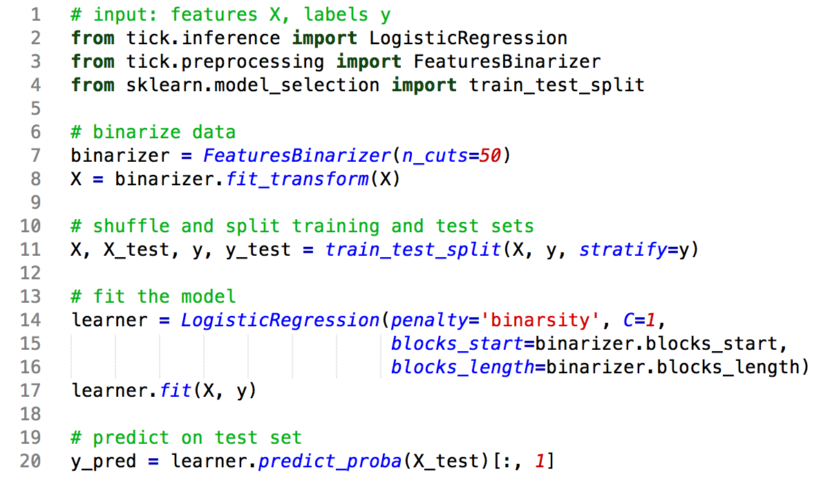
Refer to caption
Fig. 4: Sample python code for the use of binarsity with logistic regression in the tick library, with the use of the FeaturesBinarizer transformer for features binarization.

The binarsity penalization does not require a careful tuning of djd_{j} (number of bins for the one-hot encoding of raw feature jj). Indeed, past a large enough value, increasing djd_{j} even further barely changes the results since the cut-points selected by the penalization do not change anymore. This is illustrated in Figure 5, where we observe that past 5050 bins, increasing djd_{j} even further does not affect the performance, and only leads to an increase of the training time. In all our experiments, we therefore fix dj=50d_{j}=50 for j=1,…,pj=1,\ldots,p.

Fig. 5: Impact of the number of bins used in each block (djd_{j}) on the classification performance (measured by AUC) and on the training time using the “Adult” and “Default of credit card” datasets. All djd_{j} are equal for j=1,…,pj=1,\ldots,p, and we consider in all cases the best hyper-parameters selected after cross validation. We observe that past dj=50d_{j}=50 bins, performance is roughly constant, while training time strongly increases.

The results of all our experiments are reported in Figures 6 and 7. In Figure 6 we compare the performance of binarsity with the baselines on all 9 datasets, using ROC curves and the Area Under the Curve (AUC), while we report computing (training) timings in Figure 7. We observe that binarsity consistently outperforms Lasso, as well as Group L1: this highlights the importance of the TV norm within each group. The AUC of Group TV is always slightly below the one of binarsity, and more importantly it involves a much larger training time: convergence is slower for Group TV, since it does not use the linear constraint of binarsity, leading to a ill-conditioned problem (sum of binary features equals 1 in each block). Finally, binarsity outperforms also GAM and its performance is comparable in all considered examples to RF and GB, with computational timings that are orders of magnitude faster, see Figure 7. All these experiments illustrate that binarsity achieves an extremely competitive compromise between computational time and performance, compared to all considered baselines.

Fig. 6: Performance comparison using ROC curves and AUC scores (given between parenthesis) computed on test sets. The 4 last datasets contain too many examples for SVM (RBF kernel). Binarsity consistently does a better job than Lasso, Group L1, Group TV and GAM. Its performance is comparable to SVM, RF and GB but with computational timings that are orders of magnitude faster, see Figure 7.

5 Conclusion

In this paper, we introduced the binarsity penalization for one-hot encodings of continuous features. We illustrated the good statistical properties of binarsity for generalized linear models by proving non-asymptotic oracle inequalities. We conducted extensive comparisons of binarsity with state-of-the-art algorithms for binary classification on several standard datasets. Experimental results illustrate that binarsity significantly outperforms Lasso, Group L1 and Group TV penalizations and also generalized additive models, while being competitive with random forests and boosting. Moreover, it can be trained orders of magnitude faster than boosting and other ensemble methods. Even more importantly, it provides interpretability. Indeed, in addition to the raw feature selection ability of binarsity, the method pinpoints significant cut-points for all continuous feature. This leads to a much more precise and deeper understanding of the model than the one provided by Lasso on raw features. These results illustrate the fact that binarsity achieves an extremely competitive compromise between computational time and performance, compared to all considered baselines.

Fig. 7: Computing time comparisons (in seconds) between the methods on the considered datasets. Note that the time values are log\log-scaled. These timings concern the learning task for each model with the best hyper parameters selected, after the cross validation procedure. The 4 last datasets contain too many examples for the SVM with RBF kernel to be trained in a reasonable time. Roughly, binarsity is between 2 and 5 times slower than ℓ1\ell_{1} penalization on the considered datasets, but is more than 100 times faster than random forests or gradient boosting algorithms on large datasets, such as HIGGS.

6 Proofs

In this Section we gather the proofs of all the theoretical results proposed in the paper. Throughout this Section, we denote by ∂(ϕ)\partial(\phi) the subdifferential mapping of a convex function ϕ.\phi.

6.1 Proof of Proposition 1

Recall that the indicator function δj\delta_{j} is given by (6). For any fixed j=1,…,p,j=1,\ldots,p, we prove that {prox}∥⋅∥TV,w^j,∙+δj\prox_{\|\cdot\|_{\TV,\hat{w}_{j,\bullet}}+\delta_{j}} is the composition of {prox}∥⋅∥TV,w^j,∙\prox_{\|\cdot\|_{\TV,\hat{w}_{j,\bullet}}} and {prox}δj,\prox_{\delta_{j}}, namely

{prox}∥⋅∥TV,w^j,∙+δj(θj,∙)={prox}δj({prox}∥⋅∥TV,w^j,∙(θj,∙))\prox_{\|\cdot\|_{\TV,\hat{w}_{j,\bullet}}+\delta_{j}}(\theta_{j,\bullet})=\prox_{\delta_{j}}\big(\prox_{\|\cdot\|_{\TV,\hat{w}_{j,\bullet}}}(\theta_{j,\bullet})\big)

for all θj,∙∈ℝdj\theta_{j,\bullet}\in{\mathbb{R}}^{d_{j}}. Using Theorem 1 in [55], it is sufficient to show that for all θj,∙∈ℝdj,\theta_{j,\bullet}\in{\mathbb{R}}^{d_{j}}, we have

∂(‖θj,∙‖TV,w^j,∙)⊆∂(‖{prox}δj⁡(θj,∙)‖TV,w^j,∙).\partial\big(\|\theta_{j,\bullet}\|_{\TV,\hat{w}_{j,\bullet}}\big)\subseteq\partial\big(\|\prox_{\delta_{j}}(\theta_{j,\bullet})\|_{\TV,\hat{w}_{j,\bullet}}\big). (15)

We have {prox}δj⁡(θj,∙)=Πspan​{nj}⟂​(θj,∙),\prox_{\delta_{j}}(\theta_{j,\bullet})=\Pi_{\text{span}\{n_{j}\}^{\perp}}(\theta_{j,\bullet}), where Πspan​{nj}⟂​(⋅)\Pi_{\text{span}\{n_{j}\}^{\perp}}(\cdot) stands for the projection onto the orthogonal of span​{nj}\text{span}\{n_{j}\}. This projection simply writes

Πspan​{nj}⟂​(θj,∙)=θj,∙−nj⊤​θj,∙‖nj‖22​nj\Pi_{\text{span}\{n_{j}\}^{\perp}}(\theta_{j,\bullet})=\theta_{j,\bullet}-\frac{n_{j}^{\top}\theta_{j,\bullet}}{\|n_{j}\|_{2}^{2}}n_{j}

Now, let us define the dj×djd_{j}\times d_{j} matrix DjD_{j} by

Dj=[100−11⋱⋱0−11]∈ℝdj×ℝdj.{{D}_{j}}=\begin{bmatrix}1&0&&0\\ -1&1&\\ &\ddots&\ddots\\ 0&&-1&1\end{bmatrix}\in{\mathbb{R}}^{d_{j}}\times{\mathbb{R}}^{d_{j}}. (16)

We then remark that for all θj,∙∈ℝdj\theta_{j,\bullet}\in{\mathbb{R}}^{d_{j}},

‖θj,∙‖TV,w^j,∙=∑k=2djw^j,k​|θj,k−θj,k−1|=‖w^j,∙⊙Dj​θj,∙‖1.\|\theta_{j,\bullet}\|_{\TV,\hat{w}_{j,\bullet}}=\sum_{k=2}^{d_{j}}\hat{w}_{j,k}|\theta_{j,k}-\theta_{j,k-1}|=\|\hat{w}_{j,\bullet}\odot D_{j}\theta_{j,\bullet}\|_{1}. (17)

Using subdifferential calculus (see details in the proof of Proposition 2 below), one has

∂(‖θj,∙‖TV,w^j,∙)=∂(‖w^j,∙⊙Dj​θj,∙‖1)=Dj⊤​w^j,∙⊙sign⁡(Dj​θj,∙).\partial\big(\|\theta_{j,\bullet}\|_{\TV,\hat{w}_{j,\bullet}}\big)=\partial\big(\|\hat{w}_{j,\bullet}\odot{{D_{j}}}\theta_{j,\bullet}\|_{1}\big)={{D_{j}}}^{\top}\hat{w}_{j,\bullet}\odot\sgn({{D_{j}}}\theta_{j,\bullet}).

Then, the linear constraint nj⊤​θj,∙=0n_{j}^{\top}\theta_{j,\bullet}=0 entails

Dj⊤​w^j,∙⊙sign⁡(Dj​θj,∙)=Dj⊤​w^j,∙⊙sign⁡(Dj​(θj,∙−nj⊤​θj,∙‖nj‖22​nj)),{{D_{j}}}^{\top}\hat{w}_{j,\bullet}\odot\sgn({{D_{j}}}\theta_{j,\bullet})={{D_{j}}}^{\top}\hat{w}_{j,\bullet}\odot\sgn\Big({{D_{j}}}\big(\theta_{j,\bullet}-\frac{n_{j}^{\top}\theta_{j,\bullet}}{\|n_{j}\|_{2}^{2}}n_{j}\big)\Big),

which leads to (15) and concludes the proof of the Proposition. □\hfill\square

6.2 Proximal operator of the weighted TV penalization

We recall in Algorithm 2 an algorithm provided in [2] for the computation of the proximal operator of the weighted total-variation penalization

β={prox}∥⋅∥TV,w^(θ)∈argminθ∈ℝm{12∥β−θ∥22+∥θ∥TV,w^}.\beta=\prox_{\|\cdot\|_{\TV,\hat{w}}}(\theta)\in\argmin_{\theta\in{\mathbb{R}}^{m}}\Big\{\frac{1}{2}\|\beta-\theta\|_{2}^{2}+\|\theta\|_{\TV,\hat{w}}\Big\}. (18)

A quick explanation of this algorithm is as follows. The algorithm runs forwardly through the input vector (θ1,…,θm).(\theta_{1},\ldots,\theta_{m}). Using Karush-Kuhn-Tucker (KKT) optimality conditions [11], we have that at a location k,k, the weight βk\beta_{k} stays constant whenever |uk|<w^k+1|u_{k}|<\hat{w}_{k+1}, where uku_{k} is a solution to a dual problem associated to the primal problem (18). If not possible, it goes back to the last location where a jump can be introduced in β\beta, validates the current segment until this location, starts a new segment, and continues.

Algorithm 2 Proximal operator of weighted TV penalization
Input: vector θ=(θ1,…,θm)⊤∈ℝm\theta=\big(\theta_{1},\ldots,\theta_{m}\big)^{\top}\in{\mathbb{R}}^{m} and weights w^=(w^1,…,w^m)∈ℝ+m.\hat{w}=(\hat{w}_{1},\ldots,\hat{w}_{m})\in{\mathbb{R}}^{m}_{+}.
Output: vector β={prox}∥⋅∥TV,w^(θ)\beta=\prox_{\|\cdot\|_{\TV,\hat{w}}}(\theta)
1. Set k=k0=k−=k+←1k=k_{0}=k_{-}=k_{+}\leftarrow 1
βmin←θ1−w^2;βmax←θ1+w^2\qquad\beta_{\min}\leftarrow\theta_{1}-\hat{w}_{2}\ ;\ \beta_{\max}\leftarrow\theta_{1}+\hat{w}_{2}
umin←w^2;umax←−w^2\qquad u_{\min}\leftarrow\hat{w}_{2}\ ;\ u_{\max}\leftarrow-\hat{w}_{2}
2. if k=mk=m then
   βm←βmin+umin\beta_{m}\leftarrow\beta_{\min}+u_{\min}
3. if θk+1+umin<βmin−w^k+2\theta_{k+1}+u_{\min}<\beta_{\min}-\hat{w}_{k+2} then /* negative jump */
   βk0=⋯=βk−←βmin\beta_{k_{0}}=\cdots=\beta_{k_{-}}\leftarrow\beta_{\min}
   k=k0=k−=k+←k−+1k=k_{0}=k_{-}=k_{+}\leftarrow k_{-}+1
   βmin←θk−w^k+1+w^k;βmax←θk+w^k+1+w^k\beta_{\min}\leftarrow\theta_{k}-\hat{w}_{k+1}+\hat{w}_{k}\ ;\ \beta_{\max}\leftarrow\theta_{k}+\hat{w}_{k+1}+\hat{w}_{k}
   umin←w^k+1;umax←−w^k+1u_{\min}\leftarrow\hat{w}_{k+1}\ ;\ u_{\max}\leftarrow-\hat{w}_{k+1}
4. else if θk+1+umax>βmax+w^k+2\theta_{k+1}+u_{\max}>\beta_{\max}+\hat{w}_{k+2} then /* positive jump */
   βk0=…=βk+←βmax\beta_{k_{0}}=\ldots=\beta_{k_{+}}\leftarrow\beta_{\max}
   k=k0=k−=k+←k++1k=k_{0}=k_{-}=k_{+}\leftarrow k_{+}+1
   βmin←θk−w^k+1−w^k;βmax←θk+w^k+1−w^k\beta_{\min}\leftarrow\theta_{k}-\hat{w}_{k+1}-\hat{w}_{k}\ ;\ \beta_{\max}\leftarrow\theta_{k}+\hat{w}_{k+1}-\hat{w}_{k}
   umin←w^k+1;umax←−w^k+1u_{\min}\leftarrow\hat{w}_{k+1}\ ;\ u_{\max}\leftarrow-\hat{w}_{k+1}
5. else /* no jump */
   set k←k+1k\leftarrow k+1
   umin←θk+w^k+1−βmin\qquad u_{\min}\leftarrow\theta_{k}+\hat{w}_{k+1}-\beta_{\min}
   umax←θk−w^k+1−βmax\qquad u_{\max}\leftarrow\theta_{k}-\hat{w}_{k+1}-\beta_{\max} if umin≥w^k+1u_{\min}\geq\hat{w}_{k+1} then
      βmin←βmin+umin−w^k+1k−k0+1\beta_{\min}\leftarrow\beta_{\min}+\frac{u_{\min}-\hat{w}_{k+1}}{k-k_{0}+1}
      umin←w^k+1u_{\min}\leftarrow\hat{w}_{k+1}
      k−←kk_{-}\leftarrow k
   if umax≤−w^k+1u_{\max}\leq-\hat{w}_{k+1} then
      βmax←βmax+umax+w^k+1k−k0+1\beta_{\max}\leftarrow\beta_{\max}+\frac{u_{\max}+\hat{w}_{k+1}}{k-k_{0}+1}
      umax←−w^k+1u_{\max}\leftarrow-\hat{w}_{k+1}
      k+←kk_{+}\leftarrow k
6. if k<mk<m then
   go to 2.
7. if umin<0u_{\min}<0 then
   βk0=⋯=βk−←βmin\beta_{k_{0}}=\cdots=\beta_{k_{-}}\leftarrow\beta_{\min}
   k=k0=k−←k−+1k=k_{0}=k_{-}\leftarrow k_{-}+1
   βmin←θk−w^k+1+w^k\beta_{\min}\leftarrow\theta_{k}-\hat{w}_{k+1}+\hat{w}_{k}
   umin←w^k+1;umax←θk+w^k−vmaxu_{\min}\leftarrow\hat{w}_{k+1}\ ;\ u_{\max}\leftarrow\theta_{k}+\hat{w}_{k}-v_{\max}
   go to 2.
8. else if umax>0u_{\max}>0 then
   βk0=⋯=βk+←βmax\beta_{k_{0}}=\cdots=\beta_{k_{+}}\leftarrow\beta_{\max}
   k=k0=k+←k++1k=k_{0}=k_{+}\leftarrow k_{+}+1
   βmax←θk+w^k+1−w^k\beta_{\max}\leftarrow\theta_{k}+\hat{w}_{k+1}-\hat{w}_{k}
   umax←−w^k+1;umin←θk−w^k−uminu_{\max}\leftarrow-\hat{w}_{k+1}\ ;\ u_{\min}\leftarrow\theta_{k}-\hat{w}_{k}-u_{\min}
   go to 2.
9. else
   βk0=⋯=βm←βmin+umink−k0+1\beta_{k_{0}}=\cdots=\beta_{m}\leftarrow\beta_{\min}+\frac{u_{\min}}{k-k_{0}+1}

6.3 Proof of Theorem 1

The proof relies on several technical properties that are described below. From now on, we consider 𝒚=[y1⋯yn]⊤{\boldsymbol{y}}=[y_{1}\cdots y_{n}]^{\top}, 𝑿=[x1⋯xn]⊤{\boldsymbol{X}}=[x_{1}\cdots x_{n}]^{\top}, m0(𝑿)=[m0(x1)⋯m0(xn)]⊤,m^{0}({\boldsymbol{X}})=[m^{0}(x_{1})\cdots m^{0}(x_{n})]^{\top}, and recalling that OPENmθ​(xi)=θ⊤​xiB)m_{\theta}(x_{i})=\theta^{\top}x^{B}_{i}) we introduce mθ(𝑿)=[mθ(x1)⋯mθ(xn)]⊤m_{\theta}({\boldsymbol{X}})=[m_{\theta}(x_{1})\cdots m_{\theta}(x_{n})]^{\top} and b′(mθ(𝑿))=[b′(mθ(x1))⋯b′(mθ(xn))]⊤.b^{\prime}(m_{\theta}({\boldsymbol{X}}))=[b^{\prime}(m_{\theta}(x_{1}))\cdots b^{\prime}(m_{\theta}(x_{n}))]^{\top}.

Let us now define the Kullback-Leibler divergence between the true probability density funtion f0f^{0} defined in (2) and a candidate fθf_{\theta} within the generalized linear model fθ​(y|x)=exp⁡(y​mθ​(x)−b⁡(mθ​(x))CLOSEf_{\theta}(y|x)=\exp\big(ym_{\theta}(x)-b(m_{\theta}(x)) as follows

KLn​(f0,fθ)\displaystyle\mathrm{KL}_{n}(f^{0},f_{\theta}) =1n​∑i=1n𝔼ℙ𝐲|X​[log⁡f0​(yi|xi)fθ​(yi|xi)]\displaystyle=\frac{1}{n}\sum_{i=1}^{n}\mathds{E}_{\mathds{P}_{\mathbf{y}|X}}\Big[\log\frac{f^{0}(y_{i}|x_{i})}{f_{\theta}(y_{i}|x_{i})}\Big]
:=KLn​(m0​(𝑿),mθ​(𝑿)),\displaystyle:=\mathrm{KL}_{n}(m^{0}({\boldsymbol{X}}),m_{\theta}({\boldsymbol{X}})),

where ℙ𝐲|X\mathds{P}_{\mathbf{y}|X} is the joint distribution of 𝒚{\boldsymbol{y}} given 𝑿{\boldsymbol{X}}. We then have the following Lemma.

Lemma 1

The excess risk satisfies

R⁡(mθ)−R⁡(m0)=ϕ​KLn​(m0​(𝑿),mθ​(𝑿)),R(m_{\theta})-R(m^{0})=\phi\mathrm{KL}_{n}(m^{0}({\boldsymbol{X}}),m_{\theta}({\boldsymbol{X}})),

where we recall that ϕ\phi is the dispertion parameter of the generalized linear model, see (2).

Proof. If follows from the following simple computation

KLn​(m0​(𝑿),mθ​(𝑿))\displaystyle\mathrm{KL}_{n}(m^{0}({\boldsymbol{X}}),m_{\theta}({\boldsymbol{X}}))
=ϕ−1​1n​∑i=1n𝔼ℙ𝐲|X​[(−yi​mθ​(xi)+b⁡(mθ​(xi)))−(−yi​m0​(xi)+b⁡(m0​(xi)))]\displaystyle\qquad=\phi^{-1}\frac{1}{n}\sum_{i=1}^{n}\mathds{E}_{\mathds{P}_{\mathbf{y}|X}}\Big[\big(-y_{i}m_{\theta}(x_{i})+b(m_{\theta}(x_{i}))\big)-\big(-y_{i}m^{0}(x_{i})+b(m^{0}(x_{i}))\big)\Big]
=ϕ−1​(R⁡(mθ)−R⁡(m0))\displaystyle\qquad=\phi^{-1}\big(R(m_{\theta})-R(m^{0})\big)

which proves the Lemma. □\hfill\square

6.4 Optimality conditions

As explained in the following Proposition, a solution to problem (8) can be characterized using the Karush-Kuhn-Tucker (KKT) optimality conditions [11].

Proposition 2

A vector θ^=[θ^1,∙⊤⋯θ^p,∙⊤]⊤∈ℝd\hat{\theta}=[{\hat{\theta}}_{1,\bullet}^{\top}\cdots{\hat{\theta}}_{p,\bullet}^{\top}]^{\top}\in{\mathbb{R}}^{d} is an optimum of the objective function (8) if and only if there are subgradients h^=[h^j,∙]j=1,…,p∈∂‖θ^‖TV,w^\hat{h}=[\hat{h}_{j,\bullet}]_{j=1,\ldots,p}\in\partial\|\hat{\theta}\|_{\TV,\hat{w}} and g^=[g^j,∙]j=1,…,p∈∂[δj​(θ^j,∙)]j=1,…,p\hat{g}=[\hat{g}_{j,\bullet}]_{j=1,\ldots,p}\in\partial[\delta_{j}(\hat{\theta}_{j,\bullet})]_{j=1,\ldots,p} such that

∇Rn​(θ^j,∙)+h^j,∙+g^j,∙=𝟎,\nabla R_{n}(\hat{\theta}_{j,\bullet})+{\hat{h}}_{j,\bullet}+{\hat{g}}_{j,\bullet}=\mathbf{0},

where

{h^j,∙=Dj⊤​(w^j,∙⊙sign⁡(Dj​θ^j,∙))if ​j∈J⁡(θ^),h^j,∙∈Dj⊤​(w^j,∙⊙[−1,+1]dj)if ​j∈J∁​(θ^),\left\{\begin{array}[]{ll}{\hat{h}}_{j,\bullet}=D_{{j}}^{\top}\big(\hat{w}_{j,\bullet}\odot\sgn(D_{{j}}{\hat{\theta}}_{j,\bullet})\big)&\mbox{if }j\in J(\hat{\theta}),\\ {\hat{h}}_{j,\bullet}\in D_{{j}}^{\top}\big(\hat{w}_{j,\bullet}\odot{[-1,+1]}^{d_{j}}\big)&\mbox{if }j\in J^{\complement}(\hat{\theta}),\end{array}\right. (19)

and where we recall that J⁡(θ^)J(\hat{\theta}) is the support set of θ^\hat{\theta}. The subgradient g^j,∙\hat{g}_{j,\bullet} belongs to

∂(δj​(θ^j,∙))={μj,∙∈ℝdj:μj,∙⊤​θj,∙≤μj,∙⊤​θ^j,∙​ for all ​θj,∙​ such that ​nj⊤​θj,∙=0}.\partial\big(\delta_{j}(\hat{\theta}_{j,\bullet})\big)=\big\{\mu_{j,\bullet}\in{\mathbb{R}}^{d_{j}}:\mu_{j,\bullet}^{\top}\theta_{j,\bullet}\leq\mu_{j,\bullet}^{\top}\hat{\theta}_{j,\bullet}\;\text{ for all }\;\theta_{j,\bullet}\;\text{ such that }\;n_{j}^{\top}\theta_{j,\bullet}=0\big\}.

For the generalized linear model, we have

1n​(𝐗∙,jB)⊤​(b′​(mθ^​(𝐗))−𝐲)+h^j,∙+g^j,∙+f^j,∙=𝟎,\frac{1}{n}\big(\boldsymbol{X}^{{B}}_{\bullet,j}\big)^{\top}\big(b^{\prime}(m_{\hat{\theta}}({\boldsymbol{X}}))-{\boldsymbol{y}}\big)+{\hat{h}}_{j,\bullet}+\hat{g}_{j,\bullet}+\hat{f}_{j,\bullet}=\mathbf{0}, (20)

where f^=[f^j,∙]j=1,…,p\hat{f}=[{\hat{f}}_{j,\bullet}]_{j=1,\ldots,p} belongs to the normal cone of the ball Bd​(ρ).B_{d}(\rho).

Proof. The function θ↦Rn​(θ)\theta\mapsto R_{n}(\theta) is differentiable, so the subdifferential of Rn​(⋅)+bina⁡(⋅)R_{n}(\cdot)+\bina(\cdot) at a point θ=(θj,∙)j=1,…,p∈ℝd\theta=(\theta_{j,\bullet})_{j=1,\ldots,p}\in{\mathbb{R}}^{d} is given by

∂(Rn​(θ)+bina⁡(θ))=∇Rn​(θ)+∂(bina⁡(θ)),\partial(R_{n}(\theta)+\bina(\theta))=\nabla R_{n}(\theta)+\partial(\bina(\theta)),

where ∇Rn(θ)=[∂Rn​(θ)∂θ1,∙⋯∂Rn​(θ)∂θp,∙]⊤\nabla R_{n}(\theta)=\Big[\frac{\partial R_{n}(\theta)}{\partial\theta_{1,\bullet}}\cdots\frac{\partial R_{n}(\theta)}{\partial\theta_{p,\bullet}}\Big]^{\top} and

∂bina(θ)=[∂∥θ1,∙∥TV,w^1,∙+∂δj(θ1,∙)⋯∂∥θp,∙∥TV,w^p,∙+∂δj(θp,∙)]⊤.\partial\bina(\theta)=\Big[\partial\|\theta_{1,\bullet}\|_{\TV,\hat{w}_{1,\bullet}}+\partial\delta_{j}(\theta_{1,\bullet})\;\cdots\;\partial\|\theta_{p,\bullet}\|_{\TV,\hat{w}_{p,\bullet}}+\partial\delta_{j}(\theta_{p,\bullet})\Big]^{\top}.

We have ‖θj,∙‖TV,w^j,∙=‖w^j,∙⊙Dj​θj,∙‖1\|\theta_{j,\bullet}\|_{\TV,\hat{w}_{j,\bullet}}=\|\hat{w}_{j,\bullet}\odot D_{j}\theta_{j,\bullet}\|_{1} for all j=1,…,pj=1,\ldots,p. Then, by applying some properties of the subdifferential calculus, we get

∂‖θj,∙‖TV,w^j,∙={Dj⊤​sign⁡(w^j,∙⊙Dj​θj,∙) if ​Dj​θ≠𝟎,Dj⊤​(w^j,∙⊙vj) otherwise,\partial\|\theta_{j,\bullet}\|_{\TV,\hat{w}_{j,\bullet}}=\begin{cases}D_{j}^{\top}\sgn(\hat{w}_{j,\bullet}\odot D_{j}\theta_{j,\bullet})&\text{ if }D_{j}\theta\neq\mathbf{0},\\ D_{j}^{\top}\big(\hat{w}_{j,\bullet}\odot v_{j})&\text{ otherwise},\end{cases} (21)

where vj∈[−1,+1]djv_{j}\in[-1,+1]^{d_{j}} for all j=1,…,pj=1,\ldots,p. For generalized linear models, we rewrite

θ^∈argminθ∈ℝd⁡{Rn​(θ)+bina⁡(θ)+δBd​(ρ)​(θ)},\hat{\theta}\in\argmin_{\theta\in{\mathbb{R}}^{d}}\big\{R_{n}(\theta)+\bina(\theta)+\delta_{B_{d}(\rho)}(\theta)\big\}, (22)

where δBd​(ρ)\delta_{B_{d}(\rho)} is the indicator function of Bd​(ρ)B_{d}(\rho). Now, θ^=[θ^1,∙⊤⋯θ^p,∙⊤]⊤\hat{\theta}=[{\hat{\theta}}_{1,\bullet}^{\top}\cdots{\hat{\theta}}_{p,\bullet}^{\top}]^{\top} is an optimum of (22) if and only if 𝟎∈∇Rn​(mθ^)+∂‖θ^‖TV,w^+∂δBd​(ρ)​(θ^)\mathbf{0}\in\nabla R_{n}(m_{\hat{\theta}})+\partial\|\hat{\theta}\|_{\TV,\hat{w}}+\partial\delta_{B_{d}(\rho)}(\hat{\theta}). Recall that the subdifferential of δBd​(ρ)​(⋅)\delta_{B_{d}(\rho)}(\cdot) is the normal cone of Bd​(ρ)B_{d}(\rho), namely

∂δBd​(ρ)​(θ^)={η∈ℝd:η⊤​θ≤η⊤​θ^​ for all ​θ∈Bd​(ρ)}.\partial\delta_{B_{d}(\rho)}(\hat{\theta})=\big\{\eta\in{\mathbb{R}}^{d}:\eta^{\top}\theta\leq\eta^{\top}\hat{\theta}\text{ for all }\theta\in B_{d}(\rho)\}. (23)

One has

∂Rn​(θ)∂θj,∙=1n​(𝑿∙,jB)⊤​(b′​(mθ^​(𝑿))−𝒚),\frac{\partial R_{n}(\theta)}{\partial\theta_{j,\bullet}}=\frac{1}{n}(\boldsymbol{X}^{{B}}_{\bullet,j})^{\top}(b^{\prime}(m_{\hat{\theta}}({\boldsymbol{X}}))-{\boldsymbol{y}}), (24)

so that together with (24) and (23) we obtain (20), which concludes the proof of Proposition 2. □\hfill\square

6.5 Compatibility conditions

Let us define the block diagonal matrix 𝐃=diag⁡(D1,…,Dp){{\bf{D}}}=\diag({D}_{{1}},\ldots,{D}_{{p}}) with DjD_{j} defined in (16). We denote its inverse Tj{{T}_{j}} which is defined by the dj×djd_{j}\times d_{j} lower triangular matrix with entries (Tj)r,s=0({{T}_{j}})_{r,s}=0 if r<sr<s and (Tj)r,s=1({{T}_{j}})_{r,s}=1 otherwise. We set 𝐓=diag⁡(T1,…,Tp){{\bf{T}}}=\diag({T}_{{1}},\ldots,{T}_{{p}}), so that one has 𝐃−1=𝐓{\bf{D}}^{-1}={\bf{T}}.

In order to prove Theorem 1, we need the following results which give a compatibility property [51, 52, 20] for the matrix 𝐓{\bf{T}}, see Lemma 2 below and for the matrix 𝑿B​𝐓\boldsymbol{X}^{{B}}{\bf{T}}, see Lemma 3 below. For any concatenation of subsets K=[K1,…,Kp],K=[K_{1},\ldots,K_{p}], we set

Kj={τj1,…,τjbj}⊂{1,…,dj}K_{j}=\{\tau_{j}^{1},\ldots,\tau_{j}^{b_{j}}\}\subset\{1,\ldots,d_{j}\} (25)

for all j=1,…,pj=1,\ldots,p with the convention that τj0=0\tau_{j}^{0}=0 and τjbj+1=dj+1\tau_{j}^{{b_{j}}+1}=d_{j}+1.

Lemma 2

Let γ∈ℝ+d\gamma\in{\mathbb{R}}^{d}_{+} be given and K=[K1,…,Kp]K=[K_{1},\ldots,K_{p}] with KjK_{j} given by (25) for all j=1,…,pj=1,\ldots,p. Then, for every u∈ℝd\{𝟎}u\in{\mathbb{R}}^{d}\backslash\{\mathbf{0}\}, we have

‖𝐓​u‖2|‖uK⊙γK‖1−‖uK∁⊙γK∁‖1|≥κ𝐓,γ​(K),\frac{\|{\bf{T}}u\|_{2}}{|\|u_{K}\odot\gamma_{K}\|_{1}-\|u_{K^{\complement}}\odot\gamma_{K^{\complement}}\|_{1}|}\geq\kappa_{{\bf{T}},\gamma}(K),

where

κ𝐓,γ(K)={32∑j=1p∑k=1dj|γj,k+1−γj,k|2+2|Kj|∥γj,∙∥∞2Δmin,Kj−1}−1/2,\kappa_{{\bf{T}},\gamma}(K)=\bigg\{32\sum_{j=1}^{p}\sum_{k=1}^{d_{j}}|\gamma_{j,k+1}-\gamma_{j,k}|^{2}+2|K_{j}|\|\gamma_{j,\bullet}\|_{\infty}^{2}\Delta_{\min,K_{j}}^{-1}\bigg\}^{-1/2},

and Δmin,Kj=minr=1,…​bj⁡|τjrj−τjrj−1|.\Delta_{\min,K_{j}}=\min_{r=1,\ldots b^{j}}|\tau_{j}^{{r_{j}}}-\tau_{j}^{{r_{j}}-1}|.

Proof. Using Proposition 3 in [20], we have

‖uK⊙γK‖1−‖uK∁⊙γK∁‖1=∑j=1p‖uKj⊙γKj‖1−‖uKj∁⊙γKj∁‖1≤∑j=1p4​‖Tj​uj,∙‖2​{2​∑k=1dj|γj,k+1−γj,k|2+2​(bj+1)​‖γj,∙‖∞2​Δmin,Kj−1}1/2.\begin{split}&\|u_{K}\odot\gamma_{K}\|_{1}-\|u_{K^{\complement}}\odot\gamma_{K^{\complement}}\|_{1}\\ &\qquad\qquad=\sum_{j=1}^{p}\|u_{K_{j}}\odot\gamma_{K_{j}}\|_{1}-\|u_{{K_{j}}^{\complement}}\odot\gamma_{{K_{j}}^{\complement}}\|_{1}\\ &\qquad\qquad\leq\sum_{j=1}^{p}4\|T_{{j}}u_{j,\bullet}\|_{2}\bigg\{2\sum_{k=1}^{d_{j}}|\gamma_{j,k+1}-\gamma_{j,k}|^{2}+2(b_{j}+1)\|\gamma_{j,\bullet}\|_{\infty}^{2}\Delta_{\min,K_{j}}^{-1}\bigg\}^{1/2}.\end{split}

Using Hölder’s inequality for the right hand side of the last inequality gives

‖uK⊙γK‖1−‖uK∁⊙γK∁‖1≤‖𝐓​u‖2​{32​∑j=1p∑k=1dj|γj,k+1−γj,k|2+2​|Kj|​‖γj,∙‖∞2​Δmin,Kj−1}1/2,\begin{split}&\|u_{K}\odot\gamma_{K}\|_{1}-\|u_{K^{\complement}}\odot\gamma_{K^{\complement}}\|_{1}\\ &\qquad\qquad\leq\|{\bf{T}}u\|_{2}\bigg\{32\sum_{j=1}^{p}\sum_{k=1}^{d_{j}}|\gamma_{j,k+1}-\gamma_{j,k}|^{2}+2|K_{j}|\|\gamma_{j,\bullet}\|_{\infty}^{2}\Delta_{\min,K_{j}}^{-1}\bigg\}^{1/2},\end{split}

which completes the proof of the Lemma. □\hfill\square

Combining Assumption 2 and Lemma 2 allows to establish a compatibility condition satisfied by 𝑿B​𝐓\boldsymbol{X}^{{B}}{\bf{T}}.

Lemma 3

Let γ∈ℝ+d\gamma\in{\mathbb{R}}^{d}_{+} be given and K=[K1,…,Kp]K=[K_{1},\ldots,K_{p}] with KjK_{j} given by (25) for j=1,…,pj=1,\ldots,p. Then, if Assumption 2 holds, one has

infu∈𝒞1,w^​(K)\{𝟎}{‖𝑿B​𝐓​u‖2n​|‖uK⊙γK‖1−‖uK∁⊙γK∁‖1|}≥κ𝐓,γ​(K)​κ​(K),\inf\limits_{\begin{subarray}{c}u\in\mathscr{C}_{1,\hat{w}}(K)\backslash\{\mathbf{0}\}\end{subarray}}\Big\{\frac{\|\boldsymbol{X}^{{B}}{\bf{T}}u\|_{2}}{\sqrt{n}\;|\;\|u_{K}\odot\gamma_{K}\|_{1}-\|u_{K^{\complement}}\odot\gamma_{K^{\complement}}\|_{1}|}\Big\}\geq\kappa_{{\bf{T}},\gamma}(K)\kappa(K), (26)

where

𝒞1,w^​(K)={u∈ℝd:∑j=1p‖(uj,∙)Kj∁‖1,w^j,∙≤2​∑j=1p‖(uj,∙)Kj‖1,w^j,∙}.\mathscr{C}_{1,\hat{w}}(K)\stackrel{{\scriptstyle}}{{=}}\Big\{u\in{\mathbb{R}}^{d}:\sum_{j=1}^{p}\|(u_{j,\bullet})_{{K_{j}}^{\complement}}\|_{1,\hat{w}_{j,\bullet}}\leq 2\sum_{j=1}^{p}\|(u_{j,\bullet})_{K_{j}}\|_{1,\hat{w}_{j,\bullet}}\Big\}. (27)

Proof. Lemma 2 gives

‖𝑿B​𝐓​u‖2n​|‖uK⊙γK‖1−‖uK∁⊙γK∁‖1|≥κ𝐓,γ​(K)​‖𝑿B​𝐓​u‖2n​‖𝐓​u‖2.\frac{\|\boldsymbol{X}^{{B}}{\bf{T}}u\|_{2}}{\sqrt{n}|\|u_{K}\odot\gamma_{K}\|_{1}-\|u_{K^{\complement}}\odot\gamma_{K^{\complement}}\|_{1}|}\geq\kappa_{{\bf{T}},\gamma}(K)\frac{\|\boldsymbol{X}^{{B}}{\bf{T}}u\|_{2}}{\sqrt{n}\|{\bf{T}}u\|_{2}}.

Now, we note that if u∈𝒞1,w^​(K)u\in\mathscr{C}_{1,\hat{w}}(K), then 𝐓​u∈𝒞TV,w^​(K).{\bf{T}}u\in\mathscr{C}_{\TV,\hat{w}}(K). Hence, Assumption 2 entails

‖𝑿B​𝐓​u‖2n​|‖uK⊙γK‖1−‖uK∁⊙γK∁‖1|≥κ𝐓,γ​(K)​κ​(K),\frac{\|\boldsymbol{X}^{{B}}{\bf{T}}u\|_{2}}{\sqrt{n}|\|u_{K}\odot\gamma_{K}\|_{1}-\|u_{K^{\complement}}\odot\gamma_{K^{\complement}}\|_{1}|}\geq\kappa_{{\bf{T}},\gamma}(K)\kappa(K),

which concludes the proof of the Lemma. □\hfill\square

6.6 Connection between the empirical Kullback-Leibler divergence and the empirical squared norm

The next Lemma is from [3] (see Lemma 1 herein).

Lemma 4

Let φ:ℝ→ℝ\varphi:{\mathbb{R}}\rightarrow{\mathbb{R}} be a three times differentiable convex function such that for all t∈ℝ,t\in{\mathbb{R}}, |φ′′′​(t)|≤M​|φ′′​(t)||\varphi^{\prime\prime\prime}(t)|\leq M|\varphi^{\prime\prime}(t)| for some M≥0.M\geq 0. Then, for all t≥0t\geq 0, one has

φ′′​(0)M2​ψ​(−M​t)≤φ⁡(t)−φ⁡(0)−φ′​(0)​t≤φ′′​(0)M2​ψ​(M​t),\frac{\varphi^{\prime\prime}(0)}{M^{2}}\psi(-Mt)\leq\varphi(t)-\varphi(0)-\varphi^{\prime}(0)t\leq\frac{\varphi^{\prime\prime}(0)}{M^{2}}\psi(Mt),

with ψ⁡(u)=eu−u−1\psi(u)=e^{u}-u-1.

This Lemma entails the following in our setting.

Lemma 5

Under Assumption 1, one has

Ln​ψ​(−2​(Cn+ρ))4​ϕ​(Cn+ρ)2​1n​‖m0​(𝑿)−mθ​(𝑿)‖22\displaystyle\frac{L_{n}\psi(-2(C_{n}+\rho))}{4\phi(C_{n}+\rho)^{2}}\frac{1}{n}\|m^{0}({\boldsymbol{X}})-m_{\theta}({\boldsymbol{X}})\|_{2}^{2} ≤KLn​(m0​(𝑿),mθ​(𝑿)),\displaystyle\leq\mathrm{KL}_{n}(m^{0}({\boldsymbol{X}}),m_{\theta}({\boldsymbol{X}})),
Un​ψ​(2​(Cn+ρ))4​ϕ​(Cn+ρ)2​1n​‖m0​(𝑿)−mθ​(𝑿)‖22\displaystyle\frac{U_{n}\psi(2(C_{n}+\rho))}{4\phi(C_{n}+\rho)^{2}}\frac{1}{n}\|m^{0}({\boldsymbol{X}})-m_{\theta}({\boldsymbol{X}})\|_{2}^{2} ≥KLn​(m0​(𝑿),mθ​(𝑿)),\displaystyle\geq\mathrm{KL}_{n}(m^{0}({\boldsymbol{X}}),m_{\theta}({\boldsymbol{X}})),

for all θ∈Bd​(ρ)\theta\in B_{d}(\rho).

Proof. Let us consider the function Gn:ℝ→ℝG_{n}:{\mathbb{R}}\rightarrow{\mathbb{R}} defined by Gn​(t)=Rn​(m0+t​mη)G_{n}(t)=R_{n}(m^{0}+tm_{\eta}), with mηm_{\eta} to be defined later, which writes

Gn​(t)=1n​∑i=1nb⁡(m0​(xi)+t​mη​(xi))−1n​∑i=1nyi​(m0​(xi)+t​mη​(xi)).G_{n}(t)=\frac{1}{n}\sum_{i=1}^{n}b(m^{0}(x_{i})+tm_{\eta}(x_{i}))-\frac{1}{n}\sum_{i=1}^{n}y_{i}(m^{0}(x_{i})+tm_{\eta}(x_{i})).

We have

Gn′​(t)=1n​∑i=1nmη​(xi)​b′​(m0​(xi)+t​mη​(xi))−1n​∑i=1nyi​mη​(xi),Gn′′​(t)=1n​∑i=1nmη2​(xi)​b′′​(m0​(xi)+t​mη​(xi)),andGn′′′​(t)=1n​∑i=1nmη3​(xi)​b′′′​(m0​(xi)+t​mη​(xi)).\begin{split}&G^{\prime}_{n}(t)=\frac{1}{n}\sum_{i=1}^{n}m_{\eta}(x_{i})b^{\prime}(m^{0}(x_{i})+tm_{\eta}(x_{i}))-\frac{1}{n}\sum_{i=1}^{n}y_{i}m_{\eta}(x_{i}),\\ &G^{\prime\prime}_{n}(t)=\frac{1}{n}\sum_{i=1}^{n}m^{2}_{\eta}(x_{i})b^{\prime\prime}(m^{0}(x_{i})+tm_{\eta}(x_{i})),\\ \text{and}\quad&G^{\prime\prime\prime}_{n}(t)=\frac{1}{n}\sum_{i=1}^{n}m^{3}_{\eta}(x_{i})b^{\prime\prime\prime}(m^{0}(x_{i})+tm_{\eta}(x_{i})).\end{split}

Using Assumption 1, we have |Gn′′′​(t)|≤Cb​‖mη‖∞​|Gn′′​(t)||G^{\prime\prime\prime}_{n}(t)|\leq C_{b}\|m_{\eta}\|_{\infty}|G^{\prime\prime}_{n}(t)| where ‖mη‖∞:=maxi=1,…,n⁡|mη​(xi)|\|m_{\eta}\|_{\infty}:=\max\limits_{i=1,\ldots,n}|m_{\eta}(x_{i})|. Lemma 4 with M=Cb​‖mη‖∞M=C_{b}\|m_{\eta}\|_{\infty} gives

Gn′′​(0)​ψ⁡(−Cb​‖mη‖∞​t)Cb2​‖mη‖∞2≤Gn​(t)−Gn​(0)−t​Gn′​(0)≤Gn′′​(0)​ψ⁡(Cb​‖mη‖∞​t)Cb2​‖mη‖∞2G^{\prime\prime}_{n}(0)\frac{\psi(-C_{b}\|m_{\eta}\|_{\infty}t)}{C_{b}^{2}\|m_{\eta}\|_{\infty}^{2}}\leq G_{n}(t)-G_{n}(0)-tG^{\prime}_{n}(0)\leq G^{\prime\prime}_{n}(0)\frac{\psi(C_{b}\|m_{\eta}\|_{\infty}t)}{C_{b}^{2}\|m_{\eta}\|_{\infty}^{2}}

for all t≥0t\geq 0 and t=1t=1 leads to

Gn′′​(0)​ψ⁡(−Cb​‖mη‖∞)Cb2​‖mη‖∞2≤Rn​(m0+mη)−Rn​(m0)−Gn′​(0)≤Gn′′​(0)​ψ⁡(Cb​‖mη‖∞)Cb2​‖mη‖∞2.G^{\prime\prime}_{n}(0)\frac{\psi(-C_{b}\|m_{\eta}\|_{\infty})}{C_{b}^{2}\|m_{\eta}\|_{\infty}^{2}}\leq R_{n}(m^{0}+m_{\eta})-R_{n}(m^{0})-G^{\prime}_{n}(0)\leq G^{\prime\prime}_{n}(0)\frac{\psi(C_{b}\|m_{\eta}\|_{\infty})}{C_{b}^{2}\|m_{\eta}\|_{\infty}^{2}}.

An easy computation gives

−Gn′​(0)=1n​∑i=1nmη​(xi)​(yi−b′​(m0​(xi)))​ and ​Gn′′​(0)=1n​∑i=1nmη2​(xi)​b′′​(mη​(xi)),\displaystyle-G^{\prime}_{n}(0)=\frac{1}{n}\sum_{i=1}^{n}m_{\eta}(x_{i})\big(y_{i}-b^{\prime}(m^{0}(x_{i}))\big)\;\text{ and }\;G^{\prime\prime}_{n}(0)=\frac{1}{n}\sum_{i=1}^{n}m^{2}_{\eta}(x_{i})b^{\prime\prime}(m_{\eta}(x_{i})),

and since obviously 𝔼ℙ𝐲|X​[Gn′​(0)]=0\mathds{E}_{\mathds{P}_{\mathbf{y}|X}}[G_{n}^{\prime}(0)]=0, we obtain

Gn′′​(0)​ψ⁡(−Cb​‖mη‖∞)Cb2​‖mη‖∞2≤R⁡(m0+mη)−R⁡(m0)≤Gn′′​(0)​ψ⁡(Cb​‖mη‖∞)Cb2​‖mη‖∞2.\displaystyle G^{\prime\prime}_{n}(0)\frac{\psi(-C_{b}\|m_{\eta}\|_{\infty})}{C_{b}^{2}\|m_{\eta}\|_{\infty}^{2}}\leq R(m^{0}+m_{\eta})-R(m^{0})\leq G^{\prime\prime}_{n}(0)\frac{\psi(C_{b}\|m_{\eta}\|_{\infty})}{C_{b}^{2}\|m_{\eta}\|_{\infty}^{2}}.

Now, choosing mη=mθ−m0m_{\eta}=m_{\theta}-m^{0} and combining Assumption 1 with Equation (14) gives

Cb​‖mη‖∞≤Cb​maxi=1,…,n⁡(|⟨xiB,θ⟩|+|m0​(xi)|)≤Cb​(ρ+Cn).C_{b}\|m_{\eta}\|_{\infty}\leq C_{b}\max_{i=1,\ldots,n}(|\langle x_{i}^{B},\theta\rangle|+|m^{0}(x_{i})|)\leq C_{b}(\rho+C_{n}).

Hence, since x↦ψ⁡(x)/x2x\mapsto\psi(x)/x^{2} is an increasing function on ℝ+{\mathbb{R}}^{+}, we end up with

Gn′′​(0)​ψ⁡(−Cb​(Cn+ρ))Cb2​(Cn+ρ)2\displaystyle G^{\prime\prime}_{n}(0)\frac{\psi(-C_{b}(C_{n}+\rho))}{C_{b}^{2}(C_{n}+\rho)^{2}} ≤R⁡(mθ)−R⁡(m0)=ϕ​KLn​(m0​(𝑿),mθ​(𝑿)),\displaystyle\leq R(m_{\theta})-R(m_{0})=\phi\mathrm{KL}_{n}(m^{0}({\boldsymbol{X}}),m_{\theta}({\boldsymbol{X}})),
Gn′′​(0)​ψ⁡(Cb​(Cn+ρ))Cb2​(Cn+ρ)2\displaystyle G^{\prime\prime}_{n}(0)\frac{\psi(C_{b}(C_{n}+\rho))}{C_{b}^{2}(C_{n}+\rho)^{2}} ≥R⁡(mθ)−R⁡(m0)=ϕ​KLn​(m0​(𝑿),mθ​(𝑿)),\displaystyle\geq R(m_{\theta})-R(m_{0})=\phi\mathrm{KL}_{n}(m^{0}({\boldsymbol{X}}),m_{\theta}({\boldsymbol{X}})),

and since Gn′′​(0)=n−1​∑i=1n(mθ​(xi)−m0​(xi))2​b′′​(m0​(xi))G^{\prime\prime}_{n}(0)=n^{-1}\sum_{i=1}^{n}(m_{\theta}(x_{i})-m^{0}(x_{i}))^{2}b^{\prime\prime}(m^{0}(x_{i})), we obtain

Ln​ψ​(−Cb​(Cn+ρ))Cn2​ϕ​(Cn+ρ)2​1n​‖m0​(𝑿)−mθ​(𝑿)‖22\displaystyle\frac{L_{n}\psi(-C_{b}(C_{n}+\rho))}{C_{n}^{2}\phi(C_{n}+\rho)^{2}}\frac{1}{n}\|m^{0}({\boldsymbol{X}})-m_{\theta}({\boldsymbol{X}})\|_{2}^{2} ≤KLn​(m0​(𝑿),mθ​(𝑿)),\displaystyle\leq\mathrm{KL}_{n}(m^{0}({\boldsymbol{X}}),m_{\theta}({\boldsymbol{X}})),
Un​ψ​(Cb​(Cn+ρ))Cb2​ϕ​(Cn+ρ)2​1n​‖m0​(𝑿)−mθ​(𝑿)‖22\displaystyle\frac{U_{n}\psi(C_{b}(C_{n}+\rho))}{C_{b}^{2}\phi(C_{n}+\rho)^{2}}\frac{1}{n}\|m^{0}({\boldsymbol{X}})-m_{\theta}({\boldsymbol{X}})\|_{2}^{2} ≥KLn​(m0​(𝑿),mθ​(𝑿)),\displaystyle\geq\mathrm{KL}_{n}(m^{0}({\boldsymbol{X}}),m_{\theta}({\boldsymbol{X}})),

which concludes the proof of the Lemma. □\hfill\square

6.7 Proof of Theorem 1

Let us recall that

Rn​(mθ)=1n​∑i=1nb⁡(mθ​(xi))−1n​∑i=1nyi​mθ​(xi)R_{n}(m_{\theta})=\frac{1}{n}\sum_{i=1}^{n}b(m_{\theta}(x_{i}))-\frac{1}{n}\sum_{i=1}^{n}y_{i}m_{\theta}(x_{i})

for all θ∈ℝd\theta\in{\mathbb{R}}^{d} and that

θ^∈argminθ∈Bd​(ρ)⁡{Rn​(θ)+bina⁡(θ)}.\hat{\theta}\in\argmin_{\theta\in B_{d}(\rho)}\big\{R_{n}(\theta)+\bina(\theta)\big\}. (28)

Proposition 2 above entails that there is h^=[h^j,∙]j=1,…,p∈∂‖θ^‖TV,w^\hat{h}=[\hat{h}_{j,\bullet}]_{j=1,\ldots,p}\in\partial\|\hat{\theta}\|_{\TV,\hat{w}}, g^=[g^j,∙]j=1,⋯,p∈[∂δj​(θ^j,∙)]j=1,…,p\hat{g}=[\hat{g}_{j,\bullet}]_{j=1,\cdots,p}\in[\partial\delta_{j}(\hat{\theta}_{j,\bullet})]_{j=1,\ldots,p} and f^=[f^j,∙]j=1,…,p∈∂δBd​(ρ)​(θ^)\hat{f}=[\hat{f}_{j,\bullet}]_{j=1,\ldots,p}\in\partial\delta_{B_{d}(\rho)}(\hat{\theta}) such that

⟨1n​(𝑿B)⊤​(b′​(mθ^​(𝑿))−𝒚)+h^+g^+f^,θ^−θ⟩=0\Big\langle\frac{1}{n}(\boldsymbol{X}^{{B}})^{\top}(b^{\prime}(m_{\hat{\theta}}({\boldsymbol{X}}))-{\boldsymbol{y}})+\hat{h}+\hat{g}+\hat{f},\hat{\theta}-\theta\Big\rangle=0

for all θ∈ℝd\theta\in{\mathbb{R}}^{d}. This can be rewritten as

1n​⟨b′​(mθ^​(𝑿))−b′​(m0​(𝑿)),mθ^​(𝑿)−mθ​(𝑿)⟩\displaystyle\frac{1}{n}\langle b^{\prime}(m_{\hat{\theta}}({\boldsymbol{X}}))-b^{\prime}(m^{0}({\boldsymbol{X}})),m_{\hat{\theta}}({\boldsymbol{X}})-m_{\theta}({\boldsymbol{X}})\rangle
−1n​⟨𝒚−b′​(m0​(𝑿)),mθ^​(𝑿)−mθ​(𝑿)⟩+⟨h^+g^+f^,θ^−θ⟩=0.\displaystyle\qquad\qquad-\frac{1}{n}\langle{\boldsymbol{y}}-b^{\prime}(m^{0}({\boldsymbol{X}})),m_{\hat{\theta}}({\boldsymbol{X}})-m_{\theta}({\boldsymbol{X}})\rangle+\langle\hat{h}+\hat{g}+\hat{f},\hat{\theta}-\theta\rangle=0.

For any θ∈Bd​(ρ)\theta\in B_{d}(\rho) such that nj⊤​θj,∙=0n_{j}^{\top}\theta_{j,\bullet}=0 for all jj and h∈∂‖θ‖TV,w^h\in\partial\|\theta\|_{\TV,\hat{w}}, the monotony of the subdifferential mapping implies ⟨h^,θ−θ^⟩≤⟨h,θ−θ^⟩,\langle\hat{h},\theta-\hat{\theta}\rangle\leq\langle h,\theta-\hat{\theta}\rangle, ⟨g^,θ−θ^⟩≤0,\langle\hat{g},\theta-\hat{\theta}\rangle\leq 0, and ⟨f^,θ−θ^⟩≤0\langle\hat{f},\theta-\hat{\theta}\rangle\leq 0, so that

1n⟨b′(mθ^(𝑿))−b′(m0(𝑿)),mθ^(𝑿)−mθ(𝑿)⟩≤1n​⟨𝒚−b′​(m0​(𝑿)),mθ^​(𝑿)−mθ​(𝑿)⟩−⟨h,θ^−θ⟩.\begin{split}\frac{1}{n}\langle b^{\prime}(m_{\hat{\theta}}({\boldsymbol{X}}))&-b^{\prime}(m^{0}({\boldsymbol{X}})),m_{\hat{\theta}}({\boldsymbol{X}})-m_{\theta}({\boldsymbol{X}})\rangle\\ &\leq\frac{1}{n}\langle{\boldsymbol{y}}-b^{\prime}(m^{0}({\boldsymbol{X}})),m_{\hat{\theta}}({\boldsymbol{X}})-m_{\theta}({\boldsymbol{X}})\rangle-\langle h,\hat{\theta}-\theta\rangle.\end{split}{} (29)

Now, consider the function Hn:ℝ→ℝH_{n}:{\mathbb{R}}\rightarrow{\mathbb{R}} defined by

Hn​(t)=1n​∑i=1nb⁡(mθ^+t​η​(xi))−1n​∑i=1nb′​(m0​(xi))​mθ^+t​η​(xi),H_{n}(t)=\frac{1}{n}\sum_{i=1}^{n}b(m_{\hat{\theta}+t\eta}(x_{i}))-\frac{1}{n}\sum_{i=1}^{n}b^{\prime}(m^{0}(x_{i}))m_{\hat{\theta}+t\eta}(x_{i}),

where η\eta will be defined later. We use again the same arguments as in the proof of Lemma 5. We differentiate HnH_{n} three times with respect tt, so that

Hn′​(t)=1n​∑i=1nmη​(xi)​b′​(mθ^+t​η​(xi))−1n​∑i=1nb′​(m0​(xi))​mη​(xi),Hn′′​(t)=1n​∑i=1nmη2​(xi)​b′′​(mθ^+t​η​(xi)),andHn′′′​(t)=1n​∑i=1nmη3​(xi)​b′′′​(mθ^+t​η​(xi)),\begin{split}&H^{\prime}_{n}(t)=\frac{1}{n}\sum_{i=1}^{n}m_{\eta}(x_{i})b^{\prime}(m_{\hat{\theta}+t\eta}(x_{i}))-\frac{1}{n}\sum_{i=1}^{n}b^{\prime}(m^{0}(x_{i}))m_{\eta}(x_{i}),\\ &H^{\prime\prime}_{n}(t)=\frac{1}{n}\sum_{i=1}^{n}m^{2}_{\eta}(x_{i})b^{\prime\prime}(m_{\hat{\theta}+t\eta}(x_{i})),\\ \text{and}\quad&H^{\prime\prime\prime}_{n}(t)=\frac{1}{n}\sum_{i=1}^{n}m^{3}_{\eta}(x_{i})b^{\prime\prime\prime}(m_{\hat{\theta}+t\eta}(x_{i})),\end{split}

and in the way as in the proof of Lemma 5, we have |Hn′′′​(t)|≤Cb​(Cn+ρ)​|Hn′′​(t)||H^{\prime\prime\prime}_{n}(t)|\leq C_{b}(C_{n}+\rho)|H^{\prime\prime}_{n}(t)|, and Lemma 4 entails

Hn′′​(0)​ψ⁡(−Cb​t​(Cn+ρ))Cb2​(Cn+ρ)2≤Hn​(t)−Hn​(0)−t​Hn′​(0)≤Hn′′​(0)​ψ⁡(Cb​t​(Cn+ρ))Cb2​(Cn+ρ)2,H^{\prime\prime}_{n}(0)\frac{\psi(-C_{b}t(C_{n}+\rho))}{C_{b}^{2}(C_{n}+\rho)^{2}}\leq H_{n}(t)-H_{n}(0)-tH^{\prime}_{n}(0)\leq H^{\prime\prime}_{n}(0)\frac{\psi(C_{b}t(C_{n}+\rho))}{C_{b}^{2}(C_{n}+\rho)^{2}},

for all t≥0t\geq 0. Taking t=1t=1 and η=θ−θ^\eta=\theta-\hat{\theta} implies

Hn​(1)=1n​∑i=1nb⁡(mθ​(xi))−1n​∑i=1nb′​(m0​(xi))​mθ​(xi)=R⁡(mθ),\displaystyle H_{n}(1)=\frac{1}{n}\sum_{i=1}^{n}b(m_{\theta}(x_{i}))-\frac{1}{n}\sum_{i=1}^{n}b^{\prime}(m^{0}(x_{i}))m_{\theta}(x_{i})=R(m_{\theta}),
and Hn​(0)=1n​∑i=1nb⁡(mθ^​(xi))−1n​∑i=1nb′​(m0​(xi))​mθ^​(xi)=R⁡(mθ^).\displaystyle H_{n}(0)=\frac{1}{n}\sum_{i=1}^{n}b(m_{\hat{\theta}}(x_{i}))-\frac{1}{n}\sum_{i=1}^{n}b^{\prime}(m^{0}(x_{i}))m_{\hat{\theta}}(x_{i})=R(m_{\hat{\theta}}).

Moreover, we have

Hn′​(0)\displaystyle H^{\prime}_{n}(0) =1n​∑i=1n⟨xiB,θ−θ^⟩​b′​(mθ^​(xi))−1n​∑i=1nb′​(m0​(xi))​⟨xiB,θ^−θ⟩\displaystyle=\frac{1}{n}\sum_{i=1}^{n}\langle x_{i}^{B},\theta-\hat{\theta}\rangle b^{\prime}(m_{\hat{\theta}}(x_{i}))-\frac{1}{n}\sum_{i=1}^{n}b^{\prime}(m^{0}(x_{i}))\langle x_{i}^{B},\hat{\theta}-\theta\rangle
=1n​⟨b′​(mθ^​(𝑿))−b′​(m0​(𝑿)),𝑿B​(θ−θ^)⟩,\displaystyle=\frac{1}{n}\langle b^{\prime}(m_{\hat{\theta}}({\boldsymbol{X}}))-b^{\prime}(m^{0}({\boldsymbol{X}})),\boldsymbol{X}^{{B}}(\theta-\hat{\theta})\rangle,
andHn′′​(0)\displaystyle\text{and}\quad H^{\prime\prime}_{n}(0) =1n​∑i=1n⟨xiB,θ^−θ⟩2​b′′​(mθ^​(xi)).\displaystyle=\frac{1}{n}\sum_{i=1}^{n}\langle x_{i}^{B},\hat{\theta}-\theta\rangle^{2}b^{\prime\prime}(m_{\hat{\theta}}(x_{i})).

Then, we deduce that

Hn′′​(0)​ψ⁡(−Cb​(Cn+ρ))Cb2​(Cn+ρ)2≤R⁡(mθ)−R⁡(mθ^)−1n​⟨b′​(mθ^​(𝑿))−b′​(m0​(𝑿)),𝑿B​(θ−θ^)⟩=ϕ​KLn​(m0​(𝑿),mθ​(𝑿))−ϕ​KLn​(m0​(𝑿),mθ^​(𝑿))+1n​⟨b′​(mθ^​(𝑿))−b′​(m0​(𝑿)),mθ^​(𝑿)−mθ​(𝑿)⟩.\begin{split}H^{\prime\prime}_{n}(0)\frac{\psi(-C_{b}(C_{n}+\rho))}{C_{b}^{2}(C_{n}+\rho)^{2}}&\leq R(m_{\theta})-R(m_{\hat{\theta}})-\frac{1}{n}\langle b^{\prime}(m_{\hat{\theta}}({\boldsymbol{X}}))-b^{\prime}(m^{0}({\boldsymbol{X}})),\boldsymbol{X}^{{B}}(\theta-\hat{\theta})\rangle\\ &=\phi\mathrm{KL}_{n}(m^{0}({\boldsymbol{X}}),m_{\theta}({\boldsymbol{X}}))-\phi\mathrm{KL}_{n}(m^{0}({\boldsymbol{X}}),m_{\hat{\theta}}({\boldsymbol{X}}))\\ &\qquad+\frac{1}{n}\langle b^{\prime}(m_{\hat{\theta}}({\boldsymbol{X}}))-b^{\prime}(m^{0}({\boldsymbol{X}})),m_{\hat{\theta}}({\boldsymbol{X}})-m_{\theta}({\boldsymbol{X}})\rangle.\end{split}

Then, with Equation (29), one has

ϕ​KLn​(m0​(𝑿),mθ^​(𝑿))+Hn′′​(0)​ψ⁡(−Cb​(Cn+ρ))Cb2​(Cn+ρ)2≤ϕ​KLn​(m0​(𝑿),mθ​(𝑿))+1n​⟨𝒚−b′​(m0​(𝑿)),mθ^​(𝑿)−mθ​(𝑿)⟩−⟨h,θ^−θ⟩.\begin{split}&\phi\mathrm{KL}_{n}(m^{0}({\boldsymbol{X}}),m_{\hat{\theta}}({\boldsymbol{X}}))+H^{\prime\prime}_{n}(0)\frac{\psi(-C_{b}(C_{n}+\rho))}{C_{b}^{2}(C_{n}+\rho)^{2}}\\ &\qquad\leq\phi\mathrm{KL}_{n}(m^{0}({\boldsymbol{X}}),m_{\theta}({\boldsymbol{X}}))+\frac{1}{n}\langle{\boldsymbol{y}}-b^{\prime}(m^{0}({\boldsymbol{X}})),m_{\hat{\theta}}({\boldsymbol{X}})-m_{\theta}({\boldsymbol{X}})\rangle-\langle h,\hat{\theta}-\theta\rangle.\end{split} (30)

As Hn′′​(0)≥0H^{\prime\prime}_{n}(0)\geq 0, it implies that

ϕ​KLn​(m0​(𝑿),mθ^​(𝑿))\displaystyle\phi\mathrm{KL}_{n}(m^{0}({\boldsymbol{X}}),m_{\hat{\theta}}({\boldsymbol{X}})) ≤ϕ​KLn​(m0​(𝑿),mθ​(𝑿))\displaystyle\leq\phi\mathrm{KL}_{n}(m^{0}({\boldsymbol{X}}),m_{\theta}({\boldsymbol{X}}))
+1n​⟨𝒚−b′​(m0​(𝑿)),mθ^​(𝑿)−mθ​(𝑿)⟩−⟨h,θ^−θ⟩.\displaystyle\qquad+\frac{1}{n}\langle{\boldsymbol{y}}-b^{\prime}(m^{0}({\boldsymbol{X}})),m_{\hat{\theta}}({\boldsymbol{X}})-m_{\theta}({\boldsymbol{X}})\rangle-\langle h,\hat{\theta}-\theta\rangle. (31)

If 1n​⟨𝒚−b′​(m0​(𝑿)),𝑿B​(θ^−θ)⟩−⟨h,θ^−θ⟩<0,\frac{1}{n}\langle{\boldsymbol{y}}-b^{\prime}(m^{0}({\boldsymbol{X}})),\boldsymbol{X}^{{B}}(\hat{\theta}-\theta)\rangle-\langle h,\hat{\theta}-\theta\rangle<0, it follows that

KLn​(m0​(𝑿),mθ^​(𝑿))≤KLn​(m0​(𝑿),mθ​(𝑿)),\mathrm{KL}_{n}(m^{0}({\boldsymbol{X}}),m_{\hat{\theta}}({\boldsymbol{X}}))\leq\mathrm{KL}_{n}(m^{0}({\boldsymbol{X}}),m_{\theta}({\boldsymbol{X}})),

then Theorem 1 holds. From now on, let us assume that

1n​⟨𝒚−b′​(m0​(𝑿)),mθ^​(𝑿)−mθ​(𝑿)⟩−⟨h,θ^−θ⟩≥0.\frac{1}{n}\langle{\boldsymbol{y}}-b^{\prime}(m^{0}({\boldsymbol{X}})),m_{\hat{\theta}}({\boldsymbol{X}})-m_{\theta}({\boldsymbol{X}})\rangle-\langle h,\hat{\theta}-\theta\rangle\geq 0. (32)

We first derive a bound on 1n​⟨𝒚−b′​(m0​(𝑿)),mθ^​(𝑿)−mθ​(𝑿)⟩.\frac{1}{n}\langle{\boldsymbol{y}}-b^{\prime}(m^{0}({\boldsymbol{X}})),m_{\hat{\theta}}({\boldsymbol{X}})-m_{\theta}({\boldsymbol{X}})\rangle. Recall that 𝐃−1=𝐓{\bf{D}}^{-1}={\bf{T}} (see beginning of Section 6.5). We focus on finding out a bound for 1n​⟨(𝑿B​𝐓)⊤​(𝒚−b′​(m0​(𝑿))),𝐃⁡(θ^−θ)⟩.\frac{1}{n}\langle(\boldsymbol{X}^{{B}}{\bf{T}})^{\top}({\boldsymbol{y}}-b^{\prime}(m^{0}({\boldsymbol{X}}))),{\bf{D}}(\hat{\theta}-\theta)\rangle. On the one hand, one has

1n⟨(𝑿B)⊤(𝒚\displaystyle\frac{1}{n}\langle(\boldsymbol{X}^{{B}})^{\top}({\boldsymbol{y}} −b′(m0(𝑿))),θ^−θ⟩\displaystyle-b^{\prime}(m^{0}({\boldsymbol{X}}))),\hat{\theta}-\theta\rangle
=1n​⟨(𝑿B​𝐓)⊤​(𝒚−b′​(m0​(𝑿))),𝐃⁡(θ^−θ)⟩\displaystyle=\frac{1}{n}\langle(\boldsymbol{X}^{{B}}{\bf{T}})^{\top}({\boldsymbol{y}}-b^{\prime}(m^{0}({\boldsymbol{X}}))),{\bf{D}}(\hat{\theta}-\theta)\rangle
≤1n​∑j=1p∑k=1dj|((𝑿∙,jB​Tj)∙,k)⊤​(𝒚−b′​(m0​(𝑿)))|​|(Dj​(θ^j,∙−θj,∙))k|\displaystyle\leq\small{\frac{1}{n}\sum_{j=1}^{p}\sum_{k=1}^{d_{j}}|((\boldsymbol{X}^{{B}}_{\bullet,j}{T}_{j})_{\bullet,k})^{\top}({\boldsymbol{y}}-b^{\prime}(m^{0}({\boldsymbol{X}})))|\;|(D_{j}({\hat{\theta}}_{j,\bullet}-\theta_{j,\bullet}))_{k}|}

where (𝑿∙,jBTj)∙,k=[(𝑿∙,jBTj)1,k⋯(𝑿∙,jBTj)n,k]⊤∈ℝn(\boldsymbol{X}^{{B}}_{\bullet,j}{T}_{j})_{\bullet,k}=[(\boldsymbol{X}^{{B}}_{\bullet,j}{T}_{j})_{1,k}\cdots(\boldsymbol{X}^{{B}}_{\bullet,j}{T}_{j})_{n,k}]^{\top}\in{\mathbb{R}}^{n} is the kk-th column of the matrix 𝑿∙,jB​Tj.\boldsymbol{X}^{{B}}_{\bullet,j}{T}_{j}. Let us consider the event

ℰn=⋂j=1p⋂k=2djℰn,j,k, where ℰn,j,k={1n|(𝑿∙,jBTj)∙,k⊤(𝒚−b′(m0(𝑿)))|≤w^j,k},\mathcal{E}_{n}=\bigcap_{j=1}^{p}\bigcap_{k=2}^{d_{j}}\mathcal{E}_{n,j,k},\textrm{ where }\mathcal{E}_{n,j,k}=\Big\{\frac{1}{n}|(\boldsymbol{X}^{{B}}_{\bullet,j}T_{j})_{\bullet,k}^{\top}({\boldsymbol{y}}-b^{\prime}(m^{0}({\boldsymbol{X}})))|\leq\hat{w}_{j,k}\Big\},

so that, on ℰn\mathcal{E}_{n}, we have

1n⟨(𝑿B)⊤(𝒚−b′(m0(𝑿)),θ^−θ⟩\displaystyle\frac{1}{n}\langle(\boldsymbol{X}^{{B}})^{\top}({\boldsymbol{y}}-b^{\prime}(m^{0}({\boldsymbol{X}})),\hat{\theta}-\theta\rangle ≤∑j=1p∑k=1djw^j,k​|(Dj​(θ^j,∙−θj,∙))k|\displaystyle\leq\sum_{j=1}^{p}\sum_{k=1}^{d_{j}}\hat{w}_{j,k}|(D_{j}({\hat{\theta}}_{j,\bullet}-\theta_{j,\bullet}))_{k}|
≤∑j=1p‖w^j,∙⊙Dj​(θ^j,∙−θj,∙)‖1.\displaystyle\leq\sum_{j=1}^{p}\|\hat{w}_{j,\bullet}\odot D_{j}({\hat{\theta}}_{j,\bullet}-\theta_{j,\bullet})\|_{1}. (33)

On the other hand, from the definition of the subgradient [hj,∙]j=1,…,p∈∂‖θ‖TV,w^[h_{j,\bullet}]_{j=1,\ldots,p}\in\partial\|\theta\|_{\TV,\hat{w}} (see Equation (19)), one can choose hh such that

hj,k=(Dj⊤​(w^j,∙⊙sign⁡(Dj​θj,∙)))kh_{j,k}=(D_{j}^{\top}(\hat{w}_{j,\bullet}\odot\sgn(D_{{j}}{\theta}_{j,\bullet})))_{k}

for all k∈Jj​(θ)k\in J_{j}(\theta) and

hj,k=(Dj⊤​(w^j,∙⊙sign⁡(Dj​θ^j,∙))k=(Dj⊤​(w^j,∙⊙sign⁡(Dj​(θ^j,∙−θj,∙)))kCLOSECLOSEh_{j,k}=(D_{j}^{\top}(\hat{w}_{j,\bullet}\odot\sgn(D_{j}\hat{\theta}_{j,\bullet}))_{k}=(D_{j}^{\top}(\hat{w}_{j,\bullet}\odot\sgn(D_{j}(\hat{\theta}_{j,\bullet}-\theta_{j,\bullet})))_{k}

for all k∈Jj∁​(θ)k\in J_{j}^{\complement}(\theta). Using a triangle inequality and the fact that sign⁡(x)⊤​x=‖x‖1\sgn(x)^{\top}x=\|x\|_{1}, we obtain

−⟨h,θ^−θ⟩\displaystyle-\langle h,\hat{\theta}-\theta\rangle ≤∑j=1p‖(w^j,∙)Jj​(θ)⊙Dj​(θ^j,∙−θj,∙)Jj​(θ)‖1\displaystyle\leq\sum_{j=1}^{p}\|(\hat{w}_{j,\bullet})_{J_{j}(\theta)}\odot D_{{j}}(\hat{\theta}_{j,\bullet}-\theta_{j,\bullet})_{J_{j}(\theta)}\|_{1}
−∑j=1p∥(w^j,∙)Jj∁​(θ)⊙Dj(θ^j,∙−θj,∙)Jj∁​(θ)∥1\displaystyle\quad-\sum_{j=1}^{p}\|(\hat{w}_{j,\bullet})_{J^{\complement}_{j}(\theta)}\odot D_{{j}}(\hat{\theta}_{j,\bullet}-\theta_{j,\bullet})_{J^{\complement}_{j}(\theta)}\|_{1}
≤∑j=1p‖(θ^j,∙−θj,∙)Jj​(θ)‖TV,w^j,∙−∑j=1p‖(θ^j,∙−θj,∙)Jj∁​(θ)‖TV,w^j,∙.\displaystyle\leq\sum_{j=1}^{p}\|(\hat{\theta}_{j,\bullet}-\theta_{j,\bullet})_{J_{j}(\theta)}\|_{\TV,\hat{w}_{j,\bullet}}-\sum_{j=1}^{p}\|(\hat{\theta}_{j,\bullet}-\theta_{j,\bullet})_{J^{\complement}_{j}(\theta)}\|_{\TV,\hat{w}_{j,\bullet}}. (34)

Combining inequalities (33) and (34), we get

∑j=1p‖(θ^j,∙−θj,∙)Jj∁​(θ)‖TV,w^j,∙≤2​∑j=1p‖(θ^j,∙−θj,∙)Jj​(θ)‖TV,w^j,∙\sum_{j=1}^{p}\|(\hat{\theta}_{j,\bullet}-\theta_{j,\bullet})_{J^{\complement}_{j}(\theta)}\|_{\TV,\hat{w}_{j,\bullet}}\leq 2\sum_{j=1}^{p}\|(\hat{\theta}_{j,\bullet}-\theta_{j,\bullet})_{J_{j}(\theta)}\|_{\TV,\hat{w}_{j,\bullet}}

on ℰn\mathcal{E}_{n}. Hence

∑j=1p‖(w^j,∙)Jj∁​(θ)⊙Dj​(θ^j,∙−θj,∙)Jj∁​(θ)‖1≤2​∑j=1p‖(w^j,∙)Jj​(θ)⊙Dj​(θ^j,∙−θj,∙)Jj​(θ)‖1.\sum_{j=1}^{p}\|(\hat{w}_{j,\bullet})_{J^{\complement}_{j}(\theta)}\odot D_{{j}}(\hat{\theta}_{j,\bullet}-\theta_{j,\bullet})_{J^{\complement}_{j}(\theta)}\|_{1}\leq 2\sum_{j=1}^{p}\|(\hat{w}_{j,\bullet})_{J_{j}(\theta)}\odot D_{{j}}(\hat{\theta}_{j,\bullet}-\theta_{j,\bullet})_{J_{j}(\theta)}\|_{1}.

This means that

θ^−θ∈𝒞TV,w^​(J⁡(θ))​ and ​𝐃​(θ^−θ)∈𝒞1,w^​(J⁡(θ)),\hat{\theta}-\theta\in\mathscr{C}_{\TV,\hat{w}}(J(\theta))\textrm{ and }{\bf{D}}(\hat{\theta}-\theta)\in\mathscr{C}_{1,\hat{w}}(J(\theta)), (35)

see (10) and (27). Now, going back to (31) and taking into account (35), the compatibility of 𝑿B​𝐓\boldsymbol{X}^{{B}}{\bf{T}} given in Equation (26) provides the following on the event ℰn\mathcal{E}_{n}:

ϕ​KLn​(m0​(𝑿),mθ^​(𝑿))≤ϕ​KLn​(m0​(𝑿),mθ​(𝑿))+2∑j=1p∥(w^j,∙)Jj​(θ)⊙Dj(θ^j,∙−θj,∙)Jj​(θ)∥1.\begin{split}\phi\mathrm{KL}_{n}(m^{0}({\boldsymbol{X}}),m_{\hat{\theta}}({\boldsymbol{X}}))&\leq\phi\mathrm{KL}_{n}(m^{0}({\boldsymbol{X}}),m_{\theta}({\boldsymbol{X}}))\\ &\quad+2\sum_{j=1}^{p}\|(\hat{w}_{j,\bullet})_{J_{j}(\theta)}\odot D_{j}(\hat{\theta}_{j,\bullet}-\theta_{j,\bullet})_{J_{j}(\theta)}\|_{1}.\end{split}

Then

KLn​(m0​(𝑿),mθ^​(𝑿))≤KLn​(m0​(𝑿),mθ​(𝑿))+‖mθ^​(𝑿)−mθ​(𝑿)‖2n​ϕ​κ𝐓,γ^​(J⁡(θ))​κ​(J⁡(θ)),\begin{split}\mathrm{KL}_{n}(m^{0}({\boldsymbol{X}}),m_{\hat{\theta}}({\boldsymbol{X}}))&\leq\mathrm{KL}_{n}(m^{0}({\boldsymbol{X}}),m_{\theta}({\boldsymbol{X}}))+\frac{\|m_{\hat{\theta}}({\boldsymbol{X}})-m_{\theta}({\boldsymbol{X}})\|_{2}}{\sqrt{n}\,\phi\,\kappa_{\bf{T},\hat{\gamma}}(J(\theta))\kappa(J(\theta))},\end{split} (36)

where γ^=(γ^1,∙⊤,…,γ^p,∙⊤)⊤\hat{\gamma}=(\hat{\gamma}_{1,\bullet}^{\top},\ldots,\hat{\gamma}_{p,\bullet}^{\top})^{\top} is such that

γ^j,k={2​w^j,kif ​k∈Jj​(θ),0if ​k∈Jj∁​(θ),\hat{\gamma}_{j,k}=\left\{\begin{array}[]{ll}2\hat{w}_{j,k}&\mbox{if }k\in J_{j}(\theta),\\ 0&\mbox{if }k\in J_{j}^{\complement}(\theta),\end{array}\right.

for all j=1,…,pj=1,\ldots,p and

κ𝐓,γ^(J(θ))={32∑j=1p∑k=1dj|γ^j,k+1−γ^j,k|2+2|Jj(θ)|∥γ^j,∙∥∞2Δmin,Jj​(θ)−1}−1/2.\kappa_{{\bf{T}},\hat{\gamma}}(J(\theta))=\bigg\{32\sum_{j=1}^{p}\sum_{k=1}^{d_{j}}|\hat{\gamma}_{j,k+1}-\hat{\gamma}_{j,k}|^{2}+2|J_{j}(\theta)|\|\hat{\gamma}_{j,\bullet}\|_{\infty}^{2}\Delta_{\min,J_{j}(\theta)}^{-1}\bigg\}^{-1/2}.

Now, we find an upper bound for

1κ𝐓,γ^2​(J⁡(θ))=32​∑j=1p∑k=1dj|γ^j,k+1−γ^j,k|2+2​|Jj​(θ)|​‖γ^j,∙‖∞2​Δmin,Jj​(θ)−1.\frac{1}{\kappa^{2}_{{\bf{T}},\hat{\gamma}}(J(\theta))}=32\sum_{j=1}^{p}\sum_{k=1}^{d_{j}}|\hat{\gamma}_{j,k+1}-\hat{\gamma}_{j,k}|^{2}+2|J_{j}(\theta)|\|\hat{\gamma}_{j,\bullet}\|_{\infty}^{2}\Delta_{\min,J_{j}(\theta)}^{-1}.

Note that ‖γ^j,∙‖∞≤2​‖w^j,∙‖∞\|\hat{\gamma}_{j,\bullet}\|_{\infty}\leq 2\|\hat{w}_{j,\bullet}\|_{\infty}. Let us write Jj​(θ)={kj1,…,kj|Jj​(θ)|}J_{j}(\theta)=\big\{k_{j}^{1},\ldots,k_{j}^{|J_{j}(\theta)|}\big\} and set Br=[[kjr−1,kjr[[={kjr−1,kjr−1+1,…,kjr−1}B_{r}=[\![k_{j}^{r-1},k_{j}^{r}[\![\;=\{k_{j}^{r-1},k_{j}^{r-1}+1,\ldots,k_{j}^{r}-1\} for r=1,…,|Jj​(θ)|+1r=1,\ldots,|J_{j}(\theta)|+1 with the convention that kj0=0k_{j}^{0}=0 and kj|Jj​(θ)|+1=dj+1k_{j}^{|J_{j}(\theta)|+1}=d_{j}+1. Then

∑k=1dj|γ^j,k+1−γ^j,k|2=∑r=1|Jj​(θ)|+1∑k∈Br|γ^j,k+1−γ^j,k|2=∑r=1|Jj​(θ)|+1|γ^j,kjr−1+1−γ^j,kjr−1|2+|γ^j,kjr−γ^j,kjr−1|2=∑r=1|Jj​(θ)|+1γ^j,kjr−12+γ^j,kjr2=∑r=1|Jj​(θ)|2​γ^j,kjr2≤8​|Jj​(θ)|​‖(w^j,∙)Jj​(θ)‖∞2.\begin{split}\sum_{k=1}^{d_{j}}|\hat{\gamma}_{j,k+1}-\hat{\gamma}_{j,k}|^{2}&=\sum_{r=1}^{|J_{j}(\theta)|+1}\sum_{k\in B_{r}}|\hat{\gamma}_{j,k+1}-\hat{\gamma}_{j,k}|^{2}\\ &=\sum_{r=1}^{|J_{j}(\theta)|+1}|\hat{\gamma}_{j,k_{j}^{r-1}+1}-\hat{\gamma}_{j,k_{j}^{r-1}}|^{2}+|\hat{\gamma}_{j,k_{j}^{r}}-\hat{\gamma}_{j,k_{j}^{r}-1}|^{2}\\ &=\sum_{r=1}^{|J_{j}(\theta)|+1}\hat{\gamma}_{j,k_{j}^{r-1}}^{2}+\hat{\gamma}_{j,k_{j}^{r}}^{2}\\ &=\sum_{r=1}^{|J_{j}(\theta)|}2\ \hat{\gamma}_{j,k_{j}^{r}}^{2}\\ &\leq 8\ |J_{j}(\theta)|\ \|(\hat{w}_{j,\bullet})_{J_{j}(\theta)}\|_{\infty}^{2}.\end{split}

Therefore

1κ𝐓,γ^2​(J⁡(θ))≤512​∑j=1p(|Jj​(θ)|​‖(w^j,∙)Jj​(θ)‖∞2+|Jj​(θ)|​‖(w^j,∙)Jj​(θ)‖∞2​Δmin,Jj​(θ)−1)≤512​∑j=1p(1+1Δmin,Jj​(θ))​|Jj​(θ)|​‖(w^j,∙)Jj​(θ)‖∞2≤512​|J⁡(θ)|​maxj=1,…,p​‖(w^j,∙)Jj​(θ)‖∞2.\begin{split}\frac{1}{\kappa^{2}_{{\bf{T}},\hat{\gamma}}(J(\theta))}&\leq 512\sum_{j=1}^{p}\Big(|J_{j}(\theta)|\ \|(\hat{w}_{j,\bullet})_{J_{j}(\theta)}\|_{\infty}^{2}+|J_{j}(\theta)|\ \|(\hat{w}_{j,\bullet})_{J_{j}(\theta)}\|_{\infty}^{2}\Delta_{\min,J_{j}(\theta)}^{-1}\Big)\\ &\leq 512\sum_{j=1}^{p}\Big(1+\frac{1}{\Delta_{\min,J_{j}(\theta)}}\Big)|J_{j}(\theta)|\|(\hat{w}_{j,\bullet})_{J_{j}(\theta)}\|_{\infty}^{2}\\ &\leq 512|J(\theta)|\max_{j=1,\ldots,p}\|(\hat{w}_{j,\bullet})_{J_{j}(\theta)}\|_{\infty}^{2}.\end{split} (37)

Now, we use the connection between the empirical norm and Kullback-Leibler divergence. Indeed, using Lemma 5, we get

‖mθ^​(𝑿)−mθ​(𝑿)‖2n​ϕ​κ𝐓,γ^​(J⁡(θ))​κ​(J⁡(θ))\displaystyle\frac{\|m_{\hat{\theta}}({\boldsymbol{X}})-m_{\theta}({\boldsymbol{X}})\|_{2}}{\sqrt{n}\phi\kappa_{{\bf{T}},\hat{\gamma}}(J(\theta))\kappa(J(\theta))}
≤1ϕ​κ𝐓,γ^​(J⁡(θ))​κ​(J⁡(θ))​(1n​‖mθ^​(𝑿)−m0​(𝑿)‖2+1n​‖m0​(𝑿)−mθ​(𝑿)‖2)\displaystyle\quad\quad\leq\frac{1}{\sqrt{\phi}\kappa_{{\bf{T}},\hat{\gamma}}(J(\theta))\kappa(J(\theta))}\Big(\frac{1}{\sqrt{n}}\|m_{\hat{\theta}}({\boldsymbol{X}})-m^{0}({\boldsymbol{X}})\|_{2}+\frac{1}{\sqrt{n}}\|m^{0}({\boldsymbol{X}})-m_{\theta}({\boldsymbol{X}})\|_{2}\Big)
≤2ϕ​κ𝐓,γ^​(J⁡(θ))​κ​(J⁡(θ))​Cn​(ρ,Ln)​(KLn​(m0​(𝑿),mθ^​(𝑿))1/2CLOSE\displaystyle\quad\quad\leq\frac{2}{\sqrt{\phi}\kappa_{{\bf{T}},\hat{\gamma}}(J(\theta))\kappa(J(\theta))\sqrt{C_{n}(\rho,L_{n})}}\Big(\mathrm{KL}_{n}(m^{0}({\boldsymbol{X}}),m_{\hat{\theta}}({\boldsymbol{X}}))^{1/2}
OPEN+KLn​(m0​(𝑿),mθ​(𝑿))1/2),\displaystyle\qquad\qquad\qquad\qquad\qquad\qquad\qquad\qquad\qquad\qquad+\mathrm{KL}_{n}(m^{0}({\boldsymbol{X}}),m_{\theta}({\boldsymbol{X}}))^{1/2}\Big),

where we defined Cn​(ρ,Ln)=Ln​ψ​(−Cb​(Cn+ρ))Cb2​ϕ​(Cn+ρ)2C_{n}(\rho,L_{n})=\frac{L_{n}\psi(-C_{b}(C_{n}+\rho))}{C_{b}^{2}\phi(C_{n}+\rho)^{2}}, so that combined with Equation (36), we obtain

KLn​(m0​(𝑿),mθ^​(𝑿))\displaystyle\mathrm{KL}_{n}(m^{0}({\boldsymbol{X}}),m_{\hat{\theta}}({\boldsymbol{X}})) ≤KLn​(m0​(𝑿),mθ​(𝑿))\displaystyle\leq\mathrm{KL}_{n}(m^{0}({\boldsymbol{X}}),m_{\theta}({\boldsymbol{X}}))
+2ϕ​κ𝐓,γ^​(J⁡(θ))​κ​(J⁡(θ))​Cn​(ρ,Ln)​(KLn​(m0​(𝑿),mθ^​(𝑿))1/2CLOSE\displaystyle\quad+\frac{2}{\sqrt{\phi}\kappa_{{\bf{T}},\hat{\gamma}}(J(\theta))\kappa(J(\theta))\sqrt{C_{n}(\rho,L_{n})}}\big(\mathrm{KL}_{n}(m^{0}({\boldsymbol{X}}),m_{\hat{\theta}}({\boldsymbol{X}}))^{1/2}
OPEN+KLn​(m0​(𝑿),mθ​(𝑿))1/2).\displaystyle\qquad\qquad\qquad\qquad\qquad\qquad\qquad\qquad\quad+\mathrm{KL}_{n}(m^{0}({\boldsymbol{X}}),m_{\theta}({\boldsymbol{X}}))^{1/2}\big).

This inequality entails the following upper bound

KLn​(m0​(𝑿),mθ^​(𝑿))≤3​KLn​(m0​(𝑿),mθ​(𝑿))+5ϕ​κ𝐓,γ^2​(J⁡(θ))​κ2​(J⁡(θ))​Cn​(ρ,Ln),\mathrm{KL}_{n}(m^{0}({\boldsymbol{X}}),m_{\hat{\theta}}({\boldsymbol{X}}))\leq 3\mathrm{KL}_{n}(m^{0}({\boldsymbol{X}}),m_{\theta}({\boldsymbol{X}}))+\frac{5}{\phi\kappa^{2}_{{\bf{T}},\hat{\gamma}}(J(\theta))\kappa^{2}(J(\theta))C_{n}(\rho,L_{n})},

since whenever we have x≤c+b​xx\leq c+b\sqrt{x} for some x,b,c>0x,b,c>0, then x≤2​c+b2x\leq 2c+b^{2}. Introducing g⁡(x)=x2/ψ⁡(−x)=x2/(e−x+1−x)g(x)=x^{2}/\psi(-x)=x^{2}/(e^{-x}+1-x), we note that

1Cn​(ρ,Ln)=ϕLn​g​(Cb​(Cn+ρ))≤ϕLn​(Cb​(Cn+ρ)+2),\frac{1}{C_{n}(\rho,L_{n})}=\frac{\phi}{L_{n}}g(C_{b}(C_{n}+\rho))\leq\frac{\phi}{L_{n}}(C_{b}(C_{n}+\rho)+2),

since g⁡(x)≤x+2g(x)\leq x+2 for any x>0x>0. Finally, by using also (37), we end up with

KLn​(m0​(𝑿),mθ^​(𝑿))≤3​KLn​(m0​(𝑿),mθ​(𝑿))+2560​(Cb​(Cn+ρ)+2)Ln​κ2​(J⁡(θ))​|J⁡(θ)|​‖(w^j,∙)Jj​(θ)‖∞2,\mathrm{KL}_{n}(m^{0}({\boldsymbol{X}}),m_{\hat{\theta}}({\boldsymbol{X}}))\leq 3\mathrm{KL}_{n}(m^{0}({\boldsymbol{X}}),m_{\theta}({\boldsymbol{X}}))+\frac{2560(C_{b}(C_{n}+\rho)+2)}{L_{n}\kappa^{2}(J(\theta))}\;|J(\theta)|\;\|(\hat{w}_{j,\bullet})_{J_{j}(\theta)}\|_{\infty}^{2},

which is the statement provided in Theorem 1. The only thing remaining is to control the probability of the event ℰn∁\mathcal{E}_{n}^{\complement}. This is given by the following:

ℙ⁡[ℰn∁]≤∑j=1p∑k=2djℙ[1n|(𝑿B∙,jTj)∙,k⊤(𝒚−b′(m0(𝑿)))|≥w^j,k]≤∑j=1p∑k=2djℙ[∑i=1n|(𝑿B∙,jTj)i,k(yi−b′(m0(xi)))|≥nw^j,k].\begin{split}\mathds{P}[\mathcal{E}_{n}^{\complement}]&\leq\sum_{j=1}^{p}\sum_{k=2}^{d_{j}}\mathds{P}\Big[\frac{1}{n}|(\boldsymbol{X}^{{B}}_{\bullet,j}T_{j})_{\bullet,k}^{\top}({\boldsymbol{y}}-b^{\prime}(m^{0}({\boldsymbol{X}})))|\geq\hat{w}_{j,k}\Big]\\ &\leq\sum_{j=1}^{p}\sum_{k=2}^{d_{j}}\mathds{P}\Big[\sum_{i=1}^{n}|(\boldsymbol{X}^{{B}}_{\bullet,j}T_{j})_{i,k}(y_{i}-b^{\prime}(m^{0}(x_{i})))|\geq{n\hat{w}_{j,k}}\Big].\end{split}

Let ξi,j,k=(𝑿∙,jB​Tj)i,k\xi_{i,j,k}=(\boldsymbol{X}^{{B}}_{\bullet,j}{T}_{j})_{i,k} and Zi=yi−b′​(m0​(xi)).Z_{i}=y_{i}-b^{\prime}(m^{0}(x_{i})). Note that conditionally on xix_{i}, the random variables (Zi)(Z_{i}) are independent. It can be easily shown (see Theorem 5.10 in [33]) that the moment generating function of ZZ (copy of ZiZ_{i}) is given by

𝔼⁡[exp⁡(t​Z)]=exp⁡(ϕ−1​{b⁡(m0​(x)+t)−t​b′​(m0​(x)−b⁡(m0​(x)))}).\mathds{E}[\exp(tZ)]=\exp(\phi^{-1}\{b(m^{0}(x)+t)-tb^{\prime}(m^{0}(x)-b(m^{0}(x)))\}). (38)

Applying Lemma 6.1 in [44], using (38) and Assumption 1, we can derive the following Chernoff-type bounds

ℙ[∑i=1n|ξi,j,kZi|≥nw^j,k]≤2exp(−n2​w^j,k22​Un​ϕ​‖ξ∙,j,k‖22),\mathds{P}\Big[\sum_{i=1}^{n}|\xi_{i,j,k}Z_{i}|\geq n\hat{w}_{j,k}\Big]\leq 2\exp\Big(-\frac{n^{2}\hat{w}^{2}_{j,k}}{2U_{n}\phi\|\xi_{\bullet,j,k}\|_{2}^{2}}\Big), (39)

where ξ∙,j,k=[ξ1,j,k⋯ξn,j,k]⊤∈ℝn.\xi_{\bullet,j,k}=[\xi_{1,j,k}\cdots\xi_{n,j,k}]^{\top}\in{\mathbb{R}}^{n}. We have

𝑿∙,jB​Tj=[1∑k=2djx1,j,kB∑k=3djx1,j,kB⋯∑k=dj−1djx1,j,kBx1,j,djB1∑k=2djxn,j,kB∑k=3djxn,j,kB⋯∑k=dj−1djxn,j,kBxn,j,djB],{\boldsymbol{X}}^{B}_{\bullet,j}{T}_{j}=\begin{bmatrix}1&\sum_{k=2}^{d_{j}}x_{1,j,k}^{B}&\sum_{k=3}^{d_{j}}x_{1,j,k}^{B}&\cdots&\sum_{k=d_{j-1}}^{d_{j}}x_{1,j,k}^{B}&x_{1,j,d_{j}}^{B}\\ \vdots&\vdots&\vdots&&\vdots&\vdots\\ 1&\sum_{k=2}^{d_{j}}x_{n,j,k}^{B}&\sum_{k=3}^{d_{j}}x_{n,j,k}^{B}&\cdots&\sum_{k=d_{j-1}}^{d_{j}}x_{n,j,k}^{B}&x_{n,j,d_{j}}^{B}\end{bmatrix},

therefore

‖ξ∙,j,k‖22=∑i=1n(𝑿∙,jB​Tj)∙,k2=#⁡({i:xi,j∈⋃r=kdjIj,r})=n​π^j,k.\|\xi_{\bullet,j,k}\|_{2}^{2}=\sum_{i=1}^{n}({\boldsymbol{X}}^{B}_{\bullet,j}{T}_{j})^{2}_{\bullet,k}=\#\Big(\Big\{i:x_{i,j}\in\bigcup_{r=k}^{d_{j}}I_{j,r}\Big\}\Big)=n\hat{\pi}_{j,k}. (40)

So, using the weights w^j,k\hat{w}_{j,k} given by (12) together with (39) and (40), we obtain that the probability of ℰn∁\mathcal{E}_{n}^{\complement} is smaller than 2​e−A.2e^{-A}. This concludes the proof of the first part of Theorem 1. □\hfill\square

6.8 Proof of Theorem 2

First, let us note that in the least squares setting, we have R⁡(mθ)−R⁡(m0)=‖mθ−m0‖n2R(m_{\theta})-R(m^{0})=\|m_{\theta}-m^{0}\|_{n}^{2} for any θ∈ℝd\theta\in{\mathbb{R}}^{d} where ‖g‖n2=1n​∑i=1ng​(xi)2\|g\|_{n}^{2}=\frac{1}{n}\sum_{i=1}^{n}g(x_{i})^{2}, and that b⁡(y)=12​y2b(y)=\frac{1}{2}y^{2}, ϕ=σ2\phi=\sigma^{2} (noise variance) in Equation (2), and Ln=Un=1L_{n}=U_{n}=1, Cb=0C_{b}=0. Theorem 1 provides

‖mθ^−m0‖n2≤3​‖mθ−mθ0‖n2+5120​σ2κ2​(J​(θ))​|J​(θ)|​(A+log⁡d)n\|m_{\hat{\theta}}-m^{0}\|_{n}^{2}\leq 3\|m_{\theta}-m_{\theta^{0}}\|_{n}^{2}+\frac{5120\sigma^{2}}{\kappa^{2}(J(\theta))}\frac{|J(\theta)|(A+\log d)}{n}

for any θ∈ℝd\theta\in{\mathbb{R}}^{d} such that nj⊤θj∙=0n_{j}^{\top}\theta_{j\bullet}=0 and J⁡(θ)≤J∗J(\theta)\leq J_{*}. Since dj=Dd_{j}=D for all j=1,…,pj=1,\ldots,p, we have d=D​pd=Dp and

|J(θ)|=∑j=1p|{k=2,…,D:θj,k≠θj,k−1}|≤(D−1)|𝒥(θ)|∥θ∥∞≤Dp∥θ∥∞|J(\theta)|=\sum_{j=1}^{p}|\{k=2,\ldots,D:\theta_{j,k}\neq\theta_{j,k-1}\}|\leq(D-1)|\mathcal{J}(\theta)|\|\theta\|_{\infty}\leq Dp\|\theta\|_{\infty} (41)

for any θ∈ℝd\theta\in{\mathbb{R}}^{d}, where we recall that 𝒥(θ)={j=1,…,p:θj,∙≠𝟎D}\mathcal{J}(\theta)=\{j=1,\ldots,p:\theta_{j,\bullet}\neq\boldsymbol{0}_{D}\}. Also, recall that Ij,1=I1=[0,1D]I_{j,1}=I_{1}=[0,\frac{1}{D}] and Ij,k=Ik=(k−1D,kD]I_{j,k}=I_{k}=(\frac{k-1}{D},\frac{k}{D}] for k=2,…,Dk=2,\ldots,D and j=1,…,pj=1,\ldots,p. Also, we consider θ=θ∗\theta=\theta^{*}, where θj,∙∗\theta_{j,\bullet}^{*} is defined, for any j∈𝒥∗j\in\mathcal{J}_{*}, as the minimizer of

∑i=1n(∑k=1D(θj,k−mj0​(xi,j))​𝟏Ik​(xi,j))2\sum_{i=1}^{n}\Big(\sum_{k=1}^{D}(\theta_{j,k}-m_{j}^{0}(x_{i,j}))\mathbf{1}_{I_{k}}(x_{i,j})\Big)^{2}

over the set of vectors θj,∙∈ℝD\theta_{j,\bullet}\in{\mathbb{R}}^{D} satisfying nj⊤​θj,∙=0n_{j}^{\top}\theta_{j,\bullet}=0, and we put θj,∙∗=𝟎D\theta_{j,\bullet}^{*}=\boldsymbol{0}_{D} for j∉𝒥∗j\notin\mathcal{J}_{*}. It is easy to see that the solution is given by

θj,k∗=∑i=1nmj0​(xi,j)​𝟏Ik​(xi,j)nj,k,\theta_{j, k}^{*}=\frac{\sum_{i=1}^{n}m_{j}^{0}(x_{i,j})\mathbf{1}_{I_{k}}(x_{i,j})}{n_{j,k}},

where we recall that nj,k=∑i=1n𝟏Ik​(xi,j)n_{j,k}=\sum_{i=1}^{n}\mathbf{1}_{I_{k}}(x_{i,j}). Note in particular that the identifiability assumption ∑i=1nmj0​(xi,j)=0\sum_{i=1}^{n}m_{j}^{0}(x_{i,j})=0 entails that nj⊤​θj,∙∗=0n_{j}^{\top}\theta_{j,\bullet}^{*}=0. In order to control the bias term, an easy computation gives that, whenever xi,j∈Ikx_{i,j}\in I_{k}

|θj,k∗−mj0​(xi,j)|≤∑i′=1n|mj0​(xi′,j)−mj0​(xi,j)|​𝟏Ik​(xi′,j)nj,k≤L​|Ik|=LD,|\theta_{j, k}^{*}-m_{j}^{0}(x_{i,j})|\leq\frac{\sum_{i^{\prime}=1}^{n}|m_{j}^{0}(x_{i^{\prime},j})-m_{j}^{0}(x_{i,j})|\mathbf{1}_{I_{k}}(x_{i^{\prime},j})}{n_{j,k}}\leq L|I_{k}|=\frac{L}{D},

where we used the fact that mj0m_{j}^{0} is LL-Lipschitz, so that

‖mθ∗−m0‖n2\displaystyle\|m_{\theta^{*}}-m^{0}\|_{n}^{2} =1n​∑i=1n(mθ∗​(xi,j)−m0​(xi,j))2\displaystyle=\frac{1}{n}\sum_{i=1}^{n}(m_{\theta^{*}}(x_{i,j})-m^{0}(x_{i,j}))^{2}
=1n​∑i=1n(∑j∈𝒥∗∑k=1D(θj,k∗−m0​(xi,j))​𝟏Ik)2\displaystyle=\frac{1}{n}\sum_{i=1}^{n}\Big(\sum_{j\in\mathcal{J}_{*}}\sum_{k=1}^{D}(\theta_{j,k}^{*}-m^{0}(x_{i,j}))\mathbf{1}_{I_{k}}\Big)^{2}
≤|𝒥∗|n​∑i=1n(∑j∈𝒥∗∑k=1D(θj,k∗−m0​(xi,j))​𝟏Ik)2\displaystyle\leq\frac{|\mathcal{J}_{*}|}{n}\sum_{i=1}^{n}\Big(\sum_{j\in\mathcal{J}_{*}}\sum_{k=1}^{D}(\theta_{j,k}^{*}-m^{0}(x_{i,j}))\mathbf{1}_{I_{k}}\Big)^{2}
≤|𝒥∗|n​∑i=1n∑j∈𝒥∗∑k=1D(θj,k∗−m0​(xi,j))2​𝟏Ik​(xi,j)\displaystyle\leq\frac{|\mathcal{J}_{*}|}{n}\sum_{i=1}^{n}\sum_{j\in\mathcal{J}_{*}}\sum_{k=1}^{D}(\theta_{j,k}^{*}-m^{0}(x_{i,j}))^{2}\mathbf{1}_{I_{k}}(x_{i,j})
≤|𝒥∗|​∑j∈𝒥∗∑k=1DL2​|Ik|2​𝟏Ik​(xi,j)≤L2​|𝒥∗|2D2.\displaystyle\leq|\mathcal{J}_{*}|\sum_{j\in\mathcal{J}_{*}}\sum_{k=1}^{D}L^{2}|I_{k}|^{2}\mathbf{1}_{I_{k}}(x_{i,j})\leq\frac{L^{2}|\mathcal{J}_{*}|^{2}}{D^{2}}.

Note that |θj,k∗|≤‖mj0‖n,∞|\theta_{j,k}^{*}|\leq\|m_{j}^{0}\|_{n,\infty} where ‖mj0‖n,∞=maxi=1,…,n⁡|mj0​(xi,j)|\|m_{j}^{0}\|_{n,\infty}=\max_{i=1,\ldots,n}|m_{j}^{0}(x_{i,j})|. This entails that ‖θ∗‖∞≤maxj=1,…,p⁡‖mj0‖n,∞=Mn\|\theta^{*}\|_{\infty}\leq\max_{j=1,\ldots,p}\|m_{j}^{0}\|_{n,\infty}=M_{n}. So, using also (41), we end up with

‖mθ^−m0‖n2\displaystyle\|m_{\hat{\theta}}-m^{0}\|_{n}^{2} ≤3​L2​|𝒥∗|2D2+5120​σ2κ2​(J⁡(θ∗))​D​𝒥∗​Mn​(A+log⁡(D​p​Mn))n,\displaystyle\leq\frac{3L^{2}|\mathcal{J}_{*}|^{2}}{D^{2}}+\frac{5120\sigma^{2}}{\kappa^{2}(J(\theta^{*}))}\frac{D\mathcal{J}_{*}M_{n}(A+\log(DpM_{n}))}{n},

which concludes the proof Theorem 2 using D=n1/3D=n^{1/3}. □\hfill\square

References

  • [1] A. Agresti. Foundations of Linear and Generalized Linear Models. John Wiley & Sons, 2015.
  • [2] M. Z. Alaya, S. Gaïffas, and A. Guilloux. Learning the intensity of time events with change-points. Information Theory, IEEE Transactions on, 61(9):5148–5171, 2015.
  • [3] F. Bach. Self-concordant analysis for logistic regression. Electron. J. Statist., 4:384–414, 2010.
  • [4] F. Bach, R. Jenatton, J. Mairal, and G. Obozinski. Optimization with sparsity-inducing penalties. Foundations and Trends® in Machine Learning, 4(1):1–106, 2012.
  • [5] E. Bacry, M. Bompaire, S. Gaïffas, and S. Poulsen. tick: a Python library for statistical learning, with a particular emphasis on time-dependent modeling. ArXiv e-prints, July 2017.
  • [6] P. Baldi, K. Cranmer, T. Faucett, P. Sadowski, and D. Whiteson. Parameterized neural networks for high-energy physics. The European Physical Journal C, 76(5):1–7, Apr 2016.
  • [7] P. Baldi, P. Sadowski, and D. Whiteson. Searching for exotic particles in high-energy physics with deep learning. Nature communications, 5, 2014.
  • [8] H. H. Bauschke and P. L. Combettes. Convex analysis and monotone operator theory in Hilbert spaces. CMS Books in Mathematics/Ouvrages de Mathématiques de la SMC. Springer, New York, 2011.
  • [9] P. J. Bickel, Y. Ritov, and A. B. Tsybakov. Simultaneous analysis of Lasso and Dantzig selector. Ann. Statist., 37(4):1705–1732, 2009.
  • [10] J. A. Blackard and D. J. Dean. Comparative accuracies of artificial neural networks and discriminant analysis in predicting forest cover types from cartographic variables. Computers and electronics in agriculture, 24(3):131–151, 1999.
  • [11] S. Boyd and L. Vandenberghe. Convex optimization. Cambridge University Press, Cambridge, 2004.
  • [12] L. Breiman. Random forests. Mach. Learn., 45(1):5–32, 2001.
  • [13] L. Breiman, J. Friedman, R. Olshen, and C. Stone. Classification and Regression Trees. Wadsworth and Brooks, Monterey, CA, 1984.
  • [14] P. Bühlmann and S. van De Geer. Statistics for high-dimensional data. Springer Series in Statistics. Springer, Heidelberg, 2011.
  • [15] F. Bunea, A. Tsybakov, and M. Wegkamp. Sparsity oracle inequalities for the Lasso. Electron. J. Statist., 1:169–194, 2007.
  • [16] E. J. Candès and M. B. Wakin. An Introduction To Compressive Sampling. Signal Processing Magazine, IEEE, 25(2):21–30, 2008.
  • [17] E. J. Candès, M. B. Wakin, and S. P. Boyd. Enhancing sparsity by reweighted ℓ1\ell_{1} minimization. Journal of Fourier Analysis and Applications, 14(5):877–905, 2008.
  • [18] B. Chlebus and S. H. Nguyen. On finding optimal discretizations for two attributes. In Lech Polkowski and Andrzej Skowron, editors, Rough Sets and Current Trends in Computing, volume 1424 of Lecture Notes in Computer Science, pages 537–544. Springer Berlin Heidelberg, 1998.
  • [19] L. Condat. A Direct Algorithm for 1D Total Variation Denoising. IEEE Signal Processing Letters, 20(11):1054–1057, 2013.
  • [20] A. S. Dalalyan, M. Hebiri, and J. Lederer. On the prediction performance of the Lasso. Bernoulli, 23(1):552–581, 2017.
  • [21] D. L. Donoho and M. Elad. Optimally sparse representation in general (non-orthogonal) dictionaries via ℓ1\ell_{1} minimization. In PROC. NATL ACAD. SCI. USA 100 2197–202, 2002.
  • [22] D. L. Donoho and X. Huo. Uncertainty principles and ideal atomic decomposition. Information Theory, IEEE Transactions on, 47(7):2845–2862, 2001.
  • [23] J. Friedman, T. Hastie, H. Höfling, and R. Tibshirani. Pathwise coordinate optimization. Ann. Appl. Stat., 1(2):302–332, 2007.
  • [24] J. H. Friedman. Stochastic gradient boosting. Computational Statistics & Data Analysis, 38(4):367–378, 2002.
  • [25] S. Garcia, J. Luengo, J. A. Saez, V. Lopez, and F. Herrera. A survey of discretization techniques: Taxonomy and empirical analysis in supervised learning. IEEE Transactions on Knowledge and Data Engineering, 25(4):734–750, 2013.
  • [26] P. J. Green and B. W. Silverman. Nonparametric regression and generalized linear models: a roughness penalty approach. Chapman and Hall, London, 1994.
  • [27] T. Hastie and R. Tibshirani. Generalized additive models. Wiley Online Library, 1990.
  • [28] T. Hastie, R. Tibshirani, and J. Friedman. The elements of statistical learning. Springer Series in Statistics. Springer-Verlag, New York, 2001.
  • [29] Joel Horowitz, Jussi Klemelä, Enno Mammen, et al. Optimal estimation in additive regression models. Bernoulli, 12(2):271–298, 2006.
  • [30] Stéphane Ivanoff, Franck Picard, and Vincent Rivoirard. Adaptive lasso and group-lasso for functional poisson regression. The Journal of Machine Learning Research, 17(1):1903–1948, 2016.
  • [31] K. Knight and W. Fu. Asymptotics for Lasso-type estimators. Ann. Statist., 28(5):1356–1378, 2000.
  • [32] R. Kohavi. Scaling up the accuracy of naive-Bayes classifiers: A decision-tree hybrid. In KDD, volume 96, pages 202–207, 1996.
  • [33] E. L. Lehmann and G. Casella. Theory of point estimation. Springer texts in statistics. Springer, New York, 1998.
  • [34] M. Lichman. UCI Machine Learning Repository, 2013.
  • [35] H. Liu, F. Hussain, C. L. Tan, and M. Dash. Discretization: an enabling technique. Data Min. Knowl. Discov., 6(4):393–423, 2002.
  • [36] G. Lugosi and N. Vayatis. On the Bayes-risk consistency of regularized boosting methods. Annals of Statistics, pages 30–55, 2004.
  • [37] L. Meier, S. van De Geer, and P. Bühlmann. The group lasso for logistic regression. Journal of the Royal Statistical Society: Series B (Statistical Methodology), 70(1):53–71, 2008.
  • [38] Lukas Meier, Sara Van de Geer, Peter Bühlmann, et al. High-dimensional additive modeling. The Annals of Statistics, 37(6B):3779–3821, 2009.
  • [39] S. Moro, P. Cortez, and P. Rita. A data-driven approach to predict the success of bank telemarketing. Decision Support Systems, 62:22–31, 2014.
  • [40] F. Pedregosa, G. Varoquaux, A. Gramfort, V. Michel, B. Thirion, O. Grisel, M. Blondel, P. Prettenhofer, R. Weiss, V. Dubourg, J. Vanderplas, A. Passos, D. Cournapeau, M. Brucher, M. Perrot, and E. Duchesnay. Scikit-learn: Machine learning in Python. Journal of Machine Learning Research, 12:2825–2830, 2011.
  • [41] J. R. Quinlan. C4.5: Programs for Machine Learning (Morgan Kaufmann Series in Machine Learning). Morgan Kaufmann, 1 edition, 1993.
  • [42] F. Rapaport, E. Barillot, and J. P. Vert. Classification of arraycgh data using fused SVM. Bioinformatics, 24(13):i375–i382, 2008.
  • [43] Pradeep Ravikumar, John Lafferty, Han Liu, and Larry Wasserman. Sparse additive models. Journal of the Royal Statistical Society: Series B (Statistical Methodology), 71(5):1009–1030, 2009.
  • [44] P. Rigollet. Kullback Leibler aggregation and misspecified generalized linear models. Ann. Statist., 40(2):639–665, 2012.
  • [45] M. A. Russell. Mining the Social Web: Data Mining Facebook, Twitter, LinkedIn, Google+, GitHub, and More. O’Reilly Media, 2013.
  • [46] B. Schölkopf and A. J. Smola. Learning with kernels: support vector machines, regularization, optimization, and beyond. MIT press, 2002.
  • [47] V. G. Sigillito, S. P. Wing, L. V. Hutton, and K. B. Baker. Classification of radar returns from the ionosphere using neural networks. Johns Hopkins APL Technical Digest, 10(3):262–266, 1989.
  • [48] R. Tibshirani. Regression shrinkage and selection via the Lasso. J. Roy. Statist. Soc. Ser. B, 58(1):267–288, 1996.
  • [49] R. Tibshirani, M. Saunders, S. Rosset, J. Zhu, and K. Knight. Sparsity and smoothness via the fused Lasso. J. R. Stat. Soc. Ser. B Stat. Methodol., 67(1):91–108, 2005.
  • [50] Robert Tibshirani. Regression shrinkage and selection via the lasso. Journal of the Royal Statistical Society. Series B (Methodological), pages 267–288, 1996.
  • [51] S. van de Geer. High-dimensional generalized linear models and the Lasso. Ann. Statist., 36(2):614–645, 2008.
  • [52] S. van de Geer and J. Lederer. The Lasso, correlated design, and improved oracle inequalities, volume Volume 9 of Collections, pages 303–316. Institute of Mathematical Statistics, Beachwood, Ohio, USA, 2013.
  • [53] J. Wu and S. Coggeshall. Foundations of Predictive Analytics (Chapman & Hall/CRC Data Mining and Knowledge Discovery Series). Chapman & Hall/CRC, 1st edition, 2012.
  • [54] I. C. Yeh and C. H. Lien. The comparisons of data mining techniques for the predictive accuracy of probability of default of credit card clients. Expert Systems with Applications, 36(2):2473–2480, 2009.
  • [55] Y. L. Yu. On decomposing the proximal map. In C.J.C. Burges, L. Bottou, M. Welling, Z. Ghahramani, and K.Q. Weinberger, editors, Advances in Neural Information Processing Systems 26, pages 91–99. 2013.
  • [56] P. Zhao and B. Yu. On model selection consistency of Lasso. J. Mach. Learn. Res., 7:2541–2563, 2006.