On the sectional curvature along central configurations

Since Euler and Lagrange, central configurations form a main theme in studies of the $N$-body problem. Such configurations are characterized by the property that upon dropping the bodies from rest, they homothetically shrink to a total collision. Those of the 3-body problem have long been well known. They are exactly equilateral triangles due to Lagrange and certain collinear configurations found by Euler.

Every central configuration leads to homographic solutions of the $N$-body problem: ones whose configuration evolves only by rotation or scaling. Such solutions are the only explicit solutions known for the $N>2$ body problems. See the nice references [5, 14, 18] for more on central configurations.

By the planar $N$-body problem with a $1/r^{\alpha}$ potential, we mean the movement of $N$ point masses $q_{1},...,q_{N}\in\mathbb{C}$, under the equations of motion

where

is a $1/r^{\alpha}$ potential¹¹ 1 For $\alpha=0$ one normally takes $U=-\sum_{i<j}m_{i}m_{j}\log|q_{i}-q_{j}|$. Here we will consider $\alpha>0$. and $m_{k}>0$ are the masses. A central configuration is a configuration $q=(q_{1},...,q_{N})$ such that $\nabla U(q)=\lambda q$ for some $\lambda\in\mathbb{R}$.

Here we will study these central configurations using the Jacobi-Maupertuis principle. This principle reparametrizes solutions of a natural mechanical system at a fixed energy level as geodesics of a certain metric (eq. (6) below), which we call the JM-metric for short.

It is well known that the sectional curvature values of a Riemannian metric at a point determine the local behavior of nearby geodesics, governing the convergence or divergence of neighboring geodesics passing through this point. Namely, negative values imply nearby geodesics diverge more than those in a Euclidean plane, while positive values imply they diverge less (see Figure 1). These comparisons are made by examining growths of Jacobi Fields, which in turn are used to express the linearization of the geodesic flow, see for instance [2, 12, 20]. In this paper we examine some sectional curvatures of the JM-metric at central configurations.

The idea of computing curvatures of the JM-metric to obtain dynamical consequences has been explored in other works. For three equal masses subject to a strong force (with $\alpha=2$), R. Montgomery showed in [17] that, upon reducing by symmetries, the JM-curvatures are negative. This negative curvature allows a symbolic dynamics description of the orbits. Following Montgomery’s work, the authors have found in [9] similar negatively curved circumstances for the collinear and parallelogram subproblems of the 4-body strong force problem.

With regard to central configurations, in his thesis [19], Ong Chong Pin examined curvatures of the JM-metric for central force problems, and over the Lagrange relative equilibrium solution of the classic ($\alpha=1$) 3-body problem. Later, M. Barbosu and B. Elmabsout in [3] also computed some sectional curvatures along this Lagrange solution with equal masses, observing that certain energy values lead to negative sectional curvatures over this solution and noting that this negative curvature leads to ‘instability’ of these solutions. More precisely, negative sectional curvatures over a suitable set of planes along the orbit leads to exponential growth of certain Jacobi fields in forwards or backwards time. Consequently the linearized Poincaré return map of the geodesic flow may have eigenvalues off of the unit circle. This instability is called spectral instability:

There is also the weaker notion of linear instability:

Since reparametrizing orbits has no effect on the Poincaré first return map, computations using the geodesic flow of the JM-metric will lead to the same eigenvalues as those associated to the flow of the original equations of motion on a fixed energy level. The reference [11] allows a computation of the sectional curvatures through complex planes (Proposition 1 below), from which we obtain the following Barbosu-Elmabsout inspired result:

While computing these sectional curvatures we also find the following characterization interesting:

We also consider relating sectional curvatures to Saari’s conjectures (see [6]). In center of mass zero coordinates and with a Newtonian potential ($\alpha=1$), Saari’s original conjecture poses that the constancy of moment of inertia, $I:=\sum m_{k}|q_{k}|^{2}$, over a solution is equivalent to the solution being a relative equilibrium solution (see figure 4).

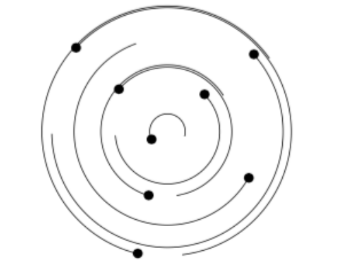
This conjecture was settled affirmatively by Moeckel [15] for three bodies, and Saari’s generalized conjecture is the same statement extended to general $1/r^{\alpha}$-potentials. Saari then posed his homographic conjecture: that constancy of

over a solution is equivalent to the solution being homographic. Recall that a solution is called homographic if the configuration, $q(t)$, remains similar to the original configuration, $q(0)$; two configurations being similar if it is possible to pass from one to the other by a scaling transformation and a rotation.

The Lagrange-Jacobi identity

shows that the ‘strong force’ potential $\alpha=2$ is exceptional, in particular Saari’s general conjecture is false for the strong force (see [21]) and for $\alpha\neq 2$ we have $\ddot{I}=const.\iff U=Const.$ Hence by restricting attention to relative equilibria, Saari’s generalized conjecture reads (for any $\alpha$):

The constancy of $U$ and $I$ over a solution is equivalent to the solution being a relative equilibrium.

Roughly speaking we seek to detect relative equilibria through sectional curvatures. To interpret Saari’s conjectures on relative equilibria geometrically we are motivated by the following plan. First we seek some distribution of planes $\sigma$ and values $C(q)$ such that $K_{q(t)}(\sigma_{q(t)})=C(q(t))$ over a solution to eq. (1) is equivalent to the constancy of $U(q(t))$ and $I(q(t))$ over the solution. Next one would seek a result similar to proposition 1 relating these curvature values to being a central configuration. Appealing as such a plan sounds, at the moment, it appears difficult and here we only explore the first step of this program.

It is worth pointing out that Proposition 3 remains true even if one replaces the condition $I(t)=$ constant by the condition that $q(t)$ is a bounded solution because, by the Lagrange-Jacobi identity with $\alpha=2$, every bounded solution must have zero energy and constant moment of inertia $I$.

As for the condition on $\alpha$ in Proposition 3, it is well known that for $\alpha\neq 2$, and again using the Lagrange-Jacobi identity that the constancy of $I$ over a solution $q(t)$ implies that the potential energy $U$ is constant over the solution.

Finally, as a direct application of Proposition 3 and Theorem 1 in [6] (which we reference here as Theorem 2 below), we obtain the following consequence.

Consider $N$ point particles of mass $m_{k}>0$ and positions $q_{k}\in\mathbb{C}$. The configuration of the system is described by the vector

where

consists of all the collisions.

The mass-weighted Hermitian inner product

allows us to write many formulae of celestial mechanics. We call its real and imaginary parts

the mass metric and mass symplectic structure on $\mathbb{C}^{N}$, which are $\mathbb{R}$-bilinear when we restrict scalar multiplication on $\mathbb{C}^{N}$ to real scalars.

The equations of motion (eq. 1) may then be written as

where $\nabla$ is the gradient for the mass metric and $U(q)$ is a $1/r^{\alpha}$ potential. These equations of motion can as well be thought of as the Hamiltonian flow of

where the mass metric allows us to translate between $T^{*}\mathbb{C}^{N}$ and $T\mathbb{C}^{N}$ via $m_{k}\dot{q}_{k}=p_{k}$. In particular the total energy $H$ is conserved over the motions. If we take the vector ${\textbf{1}}_{C}:=(1,1,...,1)\in\mathbb{C}^{N}$ we have the additional conserved quantities:

the linear momentum and angular momentum. Integrating the linear momentum once we may, as is standard, take the center of mass to be fixed at the origin

Using the mass metric, the moment of inertia, a measure of the total size of the configuration is given by

Now we consider central configurations: those with $\nabla U(q)=\lambda q$.

Fix a configuration $q$. Make the Ansatz that there exists a homographic solution $z(t)q$ of eq. (3). Then we have

where $t$ only enters in the scalars on the left hand side. It follows that

for some constant²² 2 Note that by the rotation invariance of $U$, one must have $\lambda\in\mathbb{R}$, and by $U$’s homogeneity of degree $-\alpha$, one has $sgn(\lambda)=sgn(-\alpha)$. $\lambda$, and $z(t)$ is a solution of the $1/r^{\alpha}$ central force problem:

That is to say, central configurations are exactly those which admit homographic solutions and the dynamics in the invariant plane $\mathbb{C}q$ are those of a $1/r^{\alpha}$ central force problem.

In particular, at a central configuration, we have the relative equilibria solutions of eq. (3) rotating around the origin with angular velocity $\omega\neq 0$, namely,

Lastly, we recall the Jacobi-Maupertuis reformulation of mechanics (see [2]) which asserts that the solutions to Newton’s equations at energy $H=h$ are, after a time reparameterization, precisely the geodesic equations for the Jacobi-Maupertuis metric

on the Hill region $\{q\in\mathbb{C}^{N}\setminus\triangle\,:\,h+U>0\}\subset\mathbb{C}^{N}\setminus\triangle$, and with $ds^{2}$ the mass metric.

From now on, we will consider the configuration space $\mathbb{C}^{N}\setminus\triangle$ endowed with the Jacobi-Maupertuis metric and we denote by $K_{q}(u,v)$ the sectional curvature of the JM-metric at $q$ through the plane spanned by $u,v$.

Before establishing Theorem 1 and Proposition 1, let us recall some background.

Given a Riemannian manifold, $(M^{2n},g)$ with metric compatible almost complex structure $J$, we split the complexified tangent space into the $i,-i$ eigenspaces of $J(v\otimes\lambda):=J(v)\otimes\lambda$,

In some local coordinates $(x^{j},y^{j})$ on $M$ s.t. $J(\partial_{x^{j}})=\partial_{y^{j}}$ we then have the bases for $TM^{\prime}$ and $TM^{\prime\prime}$ respectively as $\partial_{j}:=\frac{1}{2}(\partial_{x^{j}}\otimes 1-\partial_{y^{j}}\otimes i)$ and $\overline{\partial}_{j}:=\frac{1}{2}(\partial_{x^{j}}\otimes 1+\partial_{y^{j}}\otimes i)$.

Now we extend the metric $\mathbb{C}$-linearly to a $\mathbb{C}$-valued symmetric bilinear form on $TM\otimes\mathbb{C}$, by $g(v\otimes\lambda,\cdot):=\lambda g(v,\cdot)$. Using the metric compatibility of $J$ we find $g_{ij}=g(\partial_{i},\partial_{j})=0=g_{\overline{ij}}$ and

and so

where $dz^{i}=dx^{i}+idy^{i},d\overline{z}^{i}=dx^{i}-idy^{i}$ are dual to $\partial_{i},\overline{\partial}_{i}$.

The process above with the usual identification of $\mathbb{R}^{2}$ with $\mathbb{C}$ by $z=x+iy$ and $J(x,y)=(-y,x)$ corresponding to multiplication by $i$, yields the familiar operators:

With this notation note that

Let $\displaystyle{\partial=\frac{\partial}{\partial z}}$, $\displaystyle{\overline{\partial}=\frac{\partial}{\partial\overline{z}}}$. It then follows that a function $z\mapsto f(z)\in\mathbb{C}$ is holomorphic if and only if $\overline{\partial}f(z)=0.$

Let $D\subset\mathbb{C}$ be a disk containing 0 and $f:D\to M$ a holomorphic map. Let $K_{f^{*}g}$ be the Gaussian curvature of $f^{*}g$ on $D$. For $X\in T_{q}M\otimes\mathbb{C}\setminus\{0\}$, define

to be Kobayashi’s holomorphic sectional curvature. In ([11], ch. 2) Kobayashi shows that

for a unit vector $X=X^{j}\partial_{j}$ (that is $g(X,\overline{X})=1$ by extending $g$ $\mathbb{C}$-linearly) and where

To prove Proposition 1 we will make use of the following Lemmas:

In order to establish the remaining results, it will be necessary to use some auxiliary results. The first one is about the sectional curvature of the configuration space and can be found in [10].

We will see that the expression (12) becomes manageable when the plane $\sigma$ is spanned by the vectors $\dot{q}(t)$, 1. The constant vector 1 is formed by the complex numbers of the form $1+i$ in each coordinate. More specifically, we will need the following lemma for the sectional curvature on $\sigma$. Let us observe that Proposition 2 is a direct consequence of the following result.

References

- [1] A. Albouy, H. Cabral, A. Santos, Some Open problems on the classical N-body problem Celest Mech Dyn Astr (2012) 113: 369. https://doi.org/10.1007/s10569-012-9431-1
- [2] V.I. Arnold, Mathematical methods of classical mechanics, 2nd ed., New York: Springer 1989.
- [3] M. Barbosu, B. Elmabsout, Courbures de Riemann dans le problème plan des trois corps - Stabilité, C.R. Acad. Sci. Paris, t. 327, Série II b, p. 959-962, 1999.
- [4] Barutello, Vivina, Riccardo D. Jadanza, and Alessandro Portaluri.“Morse index and linear stability of the Lagrangian circular orbit in a three-body-type problem via index theory.” Archive for Rational Mechanics and Analysis 219.1 (2016): 387-444.
- [5] A. Chenciner, Collisions totales, mouvements complètement paraboliques et réduction des homothéties dans le problème des n corps, Regular and chaotic dynamics, V.3, 3, pp. 93-106 (1998).
- [6] T. Fujiwara, H. Fukuda, H. Ozaki, T. Taniguchi, Saari’s homographic conjecture for general masses in planar three-body problem under Newton potential and a strong force potential, J. Phys. A: Math. Theor. 48 (2015) 265–205.
- [7] Hu, Xijun, and Shanzhong Sun. “Morse index and stability of elliptic Lagrangian solutions in the planar three-body problem.” Advances in Mathematics 223.1 (2010): 98-119.
- [8] Hu, Xijun, and Guowei Yu. “Index Theory for Zero Energy Solutions of the Planar Anisotropic Kepler Problem.” arXiv preprint arXiv:1705.05645 (2017).
- [9] C. Jackman and J. Meléndez. Hyperbolic Shirts fit a 4-body problem, Journal of Geometry and Physics. 123 (2018) 173–183.
- [10] C. Jackman and R. Montgomery. No hyperbolic pants for the 4-body problem with strong potential, Pacific J. Math. 280 (2016), 401–410.
- [11] S. Kobayashi. Hyperbolic Complex Spaces, vol 318 of Grundlehren der matimatischen Wissenschaften, Berlin: Springer-Verlag1998.
- [12] Lee, J. M., Riemannian Manifolds: An Introduction to Curvature, Springer-Verlag Inc, (1997).
- [13] Martínez, R., Sama, A., and Simó, C. “Stability of homographic solutions of the planar three-body problem with homogeneous potentials.” Eq. Diff. 2003. 2005. 1005-1010.
- [14]
R. Moeckel. Lectures on central configurations
http://www.math.umn.edu/ rmoeckel/notes/CentralConfigurations - [15] R. Moeckel, A computer assisted proof of Saari’s conjecture for the three-body problem in . Discrete & Continuous Dynamical Systems - S, 2008, 1 (4) : 631-646.
- [16] R. Montgomery. The hyperbolic plane, three-body problems, and Mnëv’s universality theorem. Regul. Chaotic Dyn. 22 (2017), 6, 688–699.
- [17] R. Montgomery. Fitting hyperbolic pants to a three-body problem, Ergodic Theory Dynam. Systems 25 (2005), 921–947.
- [18] R. Montgomery. Blow-up for realizing homotopy classes in the three-body problem, (expository) for a school/conference held at CIMAT in Feb 2015, see arXiv:1507.07982.
- [19] Pin, Ong Chong. Curvature and mechanics. Advances in Mathematics 15.3 (1975): 269-311.
- [20] Paternain, Gabriel P. Geodesic flows. Vol. 180. Springer Science & Business Media, 2012.
- [21] G. Roberts, Some Counterexamples to Saari’s Generalized Conjecture, Transactions of the American Mathematical Society, Vol. 358 no. 1 (2005) 251 –265
- [22] Roberts, Gareth E. “Linear stability of the elliptic Lagrangian triangle solutions in the three-body problem.” Journal of Differential Equations 182.1 (2002): 191-218.