Emulating Majorana fermions and their braiding by Ising spin chains

Theoretically Majorana zero-energy states (also known as Majorana fermions) arise as a property of the Kitaev chain [1]. A physical realization is provided by a one-dimensional (1D) p-wave superconductor or – more accessible to experiment – by a semiconducting wire with strong spin-orbit interaction and proximity-induced superconductivity [2]. A fundamental elementary quantum gate, the braiding operation [3], can be performed in these systems if one uses a T-junction geometry [4]. This adiabatic manipulation (errors emerging in such manipulations are discussed in Ref. 5) allows for a restricted class of operations only; in order to construct a universal set of gates, it is necessary to expand the set of gates by non-adiabatic manipulations (for discussion and further references see Ref. 6).

Mathematically closely related is a 1D Ising chain, which can be mapped onto the Kitaev chain via the Jordan-Wigner transformation. The ideal systems are exactly equivalent, however, they differ in a crucial way in the presence of disorder [7], e.g., due to random fields. The Majorana states in the Kitaev chain are topologically protected (with exponential accuracy for long chains). I.e., local perturbations due to disorder do not lift the degeneracy of the ground states. Similarly the system remains topologically protected during the adiabatic braiding operation. In contrast, for the Ising chain a local longitudinal magnetic field does lift the degeneracy.

In spite of the lack of topological protection, simulating the physics of Majorana fermions by artificially constructed Ising chains can provide additional insight (see, e.g., the proposals of Refs. 8, 9). Short Ising chains exhibiting Majorana physics have already been simulated in optical systems [10, 11]. With present-day Josephson qubit circuits, which have reached an encouraging level of coherence, the Majorana physics could now be studied for interesting length and time scales. Several proposals on how to emulate Majorana states with Josephson circuits have already been formulated (see, e.g., Refs. 12, 13), but as a consequence of the 1D character of the Jordan-Wigner transformation the extension to a T-junction geometry, required for performing the braiding operation, remains problematic.

In this paper we first present a setup of Ising spins in a T-junction geometry which – except for the topologically protection – is equivalent to the fermionic Majorana system and allows performing the braiding operation. It relies on an extra spin-1/2 controlling the three-spin coupling in the junction. This spin also introduces Klein factors which assure that the fermionic anticommutation relations for different legs of the setup are obeyed. In addition, we propose a scheme based on a purely 1D geometry, which allows performing an operation which is equivalent to the braiding. This is achieved by attaching an extra spin-1/2 (the coupler) to the chain, such that one of the links of the Ising chain is controlled by this spin. Depending on the quantum state of the coupler, this link can be either ferromagnetic or antiferromagnetic, or a superposition thereof. The coupler should be manipulated once the ferromagnetic part of the chain, corresponding to the topological part hosting the Majorana fermions, has been moved sufficiently far away. An added advantage of this scheme is that it allows performing parity-conserving $U(1)$ rotations of the Majorana qubit by an arbitrary angle, whereas the topologically protected braiding in the fermionic system fixes this angle to discrete multiples of $\pi/4$. In this way one can construct a universal set of quantum logical gates.

Furthermore, we propose experimental implementations of our 1D setup and braiding scheme. One is based on a chain of Josephson flux qubits. They are well suited because they can be strongly coupled and the matrix element which plays the role of the transverse field can be efficiently tuned [14]. We also propose a direct translation of the 1D Ising scheme into the realm of topological wires [15, 16] hosting pairs of Majorana edge states, which allows arbitrary rotations of the Majorana qubit.

Throughout this paper we frequently use terminology appropriate for fermionic systems with topological protection, e.g., referring to topological qubits and braiding operations. This is done to emphasize the equivalence of the fermionic system and the Ising chains. We do not imply the existence of topological protection in Ising systems. But we want to stress – and this is one of the main messages of the present paper – that due to the exact mapping between the fermionic and Ising systems, topological notions have exact counterparts in the qubit chain.

Let us first recall some well-known relations between Ising chains and Majorana fermions. We consider an Ising chain described by the Hamiltonian [17]

For definiteness we consider the ferromagnetic case, $J>0$. If the perpendicular magnetic field is weak, $h(n)<J$, the ground state of a long chain, $N\rightarrow\infty$, is ferromagnetic; for strong fields the system is paramagnetic. By controlling the transverse fields $h(n)$ at each site we can define a ferromagnetic domain, which is an interval where $h(n)\ll J$, in an otherwise paramagnetic chain where $h(n)\gg J$. In the paramagnetic state, at low temperature considered here, the paramagnetic spins are ”frozen” in the state $\left|\rightarrow_{x}\right\rangle$, the ($+1$)-eigenstate of $\sigma^{x}$. The two “ground states”, $\left|\uparrow\uparrow\uparrow\right\rangle$ and $\left|\downarrow\downarrow\downarrow\right\rangle$, of the ferromagnetic section are degenerate. If $h(n)=0$ for all $n$ in the chain the degeneracy is exact ¹¹ 1 Interestingly, the degeneracy between the somewhat perturbed ground states remains exact even if $h(n)$ vanishes only at a single site, whereas in the rest of the chain $h(n)\ll J$.. For non-vanishing but small $h(n)$ a residual hybridisation between these two states decays exponentially as a function of the length of the ferromagnetic domain [17]. This remains so also when the ferromagnetic domain is surrounded by polarized paramagnetic domains (for further discussions see Ref. 18). By switching the transverse fields $h(n)$ on and off one can adiabatically control the size and position of the ferromagnetic interval, similar to the “zipping” and “unzipping” procedure described in Ref. 19.

By means of the Jordan–Wigner transformation

we can map the Ising model to a fermionic system with Hamiltonian

and fermionic Majorana operators $\chi(n)$, $\eta(n)$ satisfying the anticommutation relations

Furthermore, by introducing the local Dirac fermions $a(n)\equiv[\eta(n)+\mathrm{i}\chi(n)]/2$ and $a^{\dagger}(n)\equiv[\eta(n)-\mathrm{i}\chi(n)]/2$ we recover the Kitaev-Hamiltonian [1] of a 1D p-wave superconductor

We observe that the perpendicular magnetic field of the Ising system is equivalent to the chemical potential of the Kitaev model [1], $-2h(n)\,\hat{=}\,\mu(n)$, and the ferromagnetic coupling strength $J$ replaces the hopping matrix element $w$, which in the case described by Eq. (6) is chosen to coincide with the gap of the p-wave superconductor, $J\,\hat{=}\,w=\Delta$ (see Ref. 1).

In the Hamiltonian (4) we note that for $-2h(n)\,\hat{=}\,\mu(n)=0$ in the whole chain, the two boundary operators $\gamma_{L}\equiv\chi(1)$ and $\gamma_{R}\equiv\eta(N)$ do not appear. They represent the famous zero-energy Majorana modes [1]. For non-vanishing but weak fields, $0\neq h(n)\ll J$, the Majorana modes are no longer perfectly localized but acquire a finite extent. However, the overlap vanishes exponentially with growing length of the system. This is the origin of the topological protection of the Majorana system. For the Majorana system it is usual to introduce the Dirac fermion $d_{0}=(\gamma_{L}-\mathrm{i}\gamma_{R})/2$ and the parity operator of the zero energy subspace $P_{0}\equiv-\mathrm{i}\gamma_{R}\gamma_{L}=1-2d_{0}^{\dagger}d_{0}^{\phantom{{\dagger}}}$. Its even and odd eigenstates, $P_{0}\left|0\right\rangle=\left|0\right\rangle$, $P_{0}\left|1\right\rangle=-\left|1\right\rangle$, satisfy $d_{0}^{\dagger}\left|0\right\rangle=\left|1\right\rangle$, $d_{0}\left|1\right\rangle=\left|0\right\rangle$, $d_{0}^{\dagger}\left|1\right\rangle=d_{0}\left|0\right\rangle=0$.

In the spin system for vanishing perpendicular field the two states $\left|\uparrow\uparrow\uparrow\right\rangle$ and $\left|\downarrow\downarrow\downarrow\right\rangle$ are degenerate and span a qubit space. For non-vanishing but weak fields the spin states are no longer perfectly ferromagnetic. However, if the ferromagnetic domain is long the ensuing hybridisation is exponentially suppressed. The mapping between the Majorana and the spin system is achieved by $\gamma_{L}=\chi(1)=\sigma^{z}(1)$ and $\gamma_{R}=\eta(N)=\sigma^{y}(N)\prod_{p=1}^{N-1}\sigma^{x}(p)=-\mathrm{i}\sigma^{z}(N)P$, where the total parity operator of the chain reads $P\equiv\prod_{p=1}^{N}\sigma^{x}(p)$. Thus we have

I.e., $\gamma_{L}\,\hat{=}\,\tau^{z}$ and $\gamma_{R}\,\hat{=}\,\tau^{y}$ correspond to two non-commuting spin-like operators (Pauli matrices) in the 2-dimensional subspace of ferromagnetic states. From here we also find the mapping between the even and odd eigenstates of the Majorana system and the ferromagnetic states of the spin system

Finally we mention that the non-topological state of the Majorana system, found for $|\mu|\geq 2|w|$, corresponds to the paramagnetic phase of the spin system, $|h|\geq|J|$.

For strictly 1D setups the mapping between an Ising chain and the Majorana system is exact. However, for the latter the braiding operation has been recognized as an essential tool, which can be achieved in a T-junction geometry. In order to emulate this operation we consider now 3 Ising chains coupled to each other as shown in Fig. 1. The Hamiltonian of each of the chains with label $\alpha=1,2,3$ and – for convenience – the site index $n$ counting from the junction, reads

One could try to extend the Jordan–Wigner transformation by introducing a global 1D ordering, i.e., numbering the sites in all three chains in some order. However, any such order is artificial and leads to non-local interactions, thus precluding mapping to a fermionic system with a quadratic Hamiltonian and braiding by established procedures [20]. An alternative is provided by a modified Jordan-Wigner transformation similar to the one proposed in Ref. 21. It introduces an extra spin, denoted by the Pauli matrices $S^{\alpha}$,

This extra spin provides Klein factors. The Hamiltonian of each chain is again of the form (1), while due to the extra operators $S^{\alpha}$ also the Majorana operators belonging to different chains anticommute. Thus, we have properly “fermionized” the whole system. In what follows it will be important to know the commutation relations between $S^{\alpha}$ and the Majorana operators (10) and (11),

This doubles the Hilbert space and creates effectively two equivalent copies of the system. With this extension one arrives at a simple fermionic description.

To proceed one could introduce additional Ising couplings between the first spins of each chain, as indicated in the left panel of Fig. 1, with Hamiltonian

In the fermionic representation this becomes

This form suggests a connection to the Kondo model, which was explored in Refs. 22, 23 and is most interesting for critical Ising chains with $h\approx J$. This connection may not be obvious, since some spin and fermionic operators do not commute with each other, cf. Eq. (12). To overcome this obstacle, one can proceed with the modified Jordan-Wigner transformation [21]. Since this approach is irrelevant for our purposes it will not be discussed here any further. Furthermore, we note that the simple Ising coupling (13) between the chains does not lead to a quadratic Hamiltonian in terms of Majorana fermions. This will influence protocols intended to simulate braiding-type protocols in such systems. In fact, as can be seen in the spin description, the braiding-type procedure used in Ref. 20 does not produce a desired qubit operation, rather it may lead to an identity operation.

As an alternative we suggest proceeding with another coupling Hamiltonian, as illustrated in the right panel of Fig. 1. It relies on a three-spin interaction with an extra spin-1/2 with components $S^{\alpha}$ in the junction. We call this extra spin the “coupler”. The interaction between the chains is described by the Hamiltonian

with summation over mutually distinct $\alpha$, $\beta$, $\gamma$ and $J_{\alpha\beta}=J_{\beta\alpha}$. The fermionic version of this coupling reads

with the Levi-Civita symbol $\epsilon^{\alpha\beta\gamma}$. Thus the coupling (15) leads to a quadratic fermionic Hamiltonian; cf. a similar discussion in Ref. 21 and three-spin couplings employed in Refs. 10, 11. This ensures that braiding can be performed by standard methods [4]. Note that the operators $S^{\alpha}$ disappear from the Hamiltonian. Nevertheless, as we will see below, the spin is not decoupled since the components $S^{\alpha}$ do not, in general, commute with $H_{\rm int}^{S}$ (cf. Eqs. (12)).

To simulate braiding we follow the braiding protocol for a T-junction geometry as described in Ref. 4. We begin with the state with only one ferromagnetic domain (representing the topological section) placed in the left leg, $\alpha=1$. In the first stage of the operation the ferromagnetic domain is transported adiabatically through the upper link of the coupler region to the right leg, $\alpha=2$, then through the right link to the lower leg, $\alpha=3$, and finally through the left link back to the left leg. At each stage of the protocol only one of three couplings $J_{\alpha\beta}$ is switched on while the ferromagnetic ($\sim$topological) domain is transported through the coupler. Let us consider the effect of these operations, first in the spin language. During the first stage, if $S^{3}=+1$, the state of the ferromagnetic region (qubit) is conserved, while for $S^{3}=-1$ all spins are switched between up- and down. To proceed it is useful to move to the Heisenberg picture and record what happens to the operators. We define in the (low-energy) qubit space the Pauli matrix operators $\hat{\tau}^{x,y,z}$, in the up-down ($\left|\uparrow\uparrow\uparrow\right\rangle$, $\left|\downarrow\downarrow\downarrow\right\rangle$) basis. In the Heisenberg picture, during the first stage $\tau^{x}$ and $S^{3}$ are conserved, while $\tau^{y,z}\to S^{3}\tau^{y,z}$ and $S^{1,2}\to\tau^{x}S^{1,2}$. In the second and third stages transformations are similar, with the part of $S^{3}$ played by $S^{1}$ and $S^{2}$, respectively. The combination of all three stages yields

whereas $\tau^{x}$ and the three coupler spin components $S^{1}$, $S^{2}$, $S^{3}$ are preserved. After the three stages the coupler spin is again disentangled from the qubit, although they were entangled during the process, and the braiding operation is achieved (i.e., a $\pi/2$ $x$-rotation in the language of pseudospin $\boldsymbol{\tau}$). Indeed, within the doubly degenerate ground state the two fermionic Majorana operators, $\gamma_{\rm in}=\tau^{z}$ and $\gamma_{\rm out}=\tau^{y}$ are interchanged (see Eqs. (2,3) and after Eq. (1)): $\gamma_{\rm in}\to\gamma_{\rm out}$, $\gamma_{\rm out}\to-\gamma_{\rm in}$. (Since the notation $\gamma_{L}$ and $\gamma_{R}$, used in Section II for Majorana zero-modes becomes ambiguous in the T-junction geometry we use here the notation $\gamma_{\rm in}$ for the Majorana zero-mode which is closest to the junction and $\gamma_{\rm out}$ for the one that is further away.)

We conclude that the coupling (15) allows simulating the braiding protocol of Majorana systems in a spin system, which is one of the main messages of this paper. On the other hand, we can not exclude that the coupling is difficult to realize in an experiment. Fortunately, there are further possibilities, including one which is based on a strictly 1D geometry, which will be discussed in the following section.

Based on the considerations presented above we suggest an alternative approach replacing the braiding, based on a purely one-dimensional geometry as displayed in Fig. 2. I.e., we consider a system with only two chains ($\alpha=1$ and $2$), with a 3-spin interaction coupling the two chains, $H_{\rm int}^{S}=-J_{12}\sigma_{1}^{z}(1)\sigma_{2}^{z}(1)\,S^{3}$. Effectively, the transport of the ferromagnetic ($\sim$topological) domain through all three components $S^{1}$, $S^{2}$, and $S^{3}$, described for the T-junction geometry, can be replaced by transport through a single spin provided we rotate the state of the coupler between various stages of the protocol. Depending on the angles of these rotations, the following protocol also provides a generalization of the single-domain braiding protocol, namely allowing for an arbitrary rotation angle, cf. below. Moreover, a single intermediate rotation of the coupler spin is sufficient, as we will demonstrate.

The braiding protocol in terms of spins described in the previous section showed the following: When the ferromagnetic interval is adiabatically transported through the coupler, the spins of the domain remain intact if the coupling is ferromagnetic ($S^{\gamma}=+1$) and flip if the coupling is antiferromagnetic ($S^{\gamma}=-1$). If the coupler is in a superposition of the two states, the coupler and the ferromagnetic domain become entangled. In the 1D geometry, one again should first pull the ferromagnetic region (qubit) through the special Ising link which is controlled by the coupler spin $S^{3}$. The stages controlled by $S^{1}$- and $S^{2}$ are no longer available, which limits the accessible possibilities. However, one could emulate various coupler-spin components by rotations of the coupler spin between the pulling operations. Thus, for instance, one can achieve a braiding-type operation by pulling the qubit through the coupler three times with proper coupler-spin rotations in between. The rotations should be chosen in such a manner that three spin components are involved in sequence. This statement can be also confirmed by a direct calculation of the evolution of $\boldsymbol{\tau}$ and $\bf S$ operators. Moreover, one can achieve a a braiding-type operation also with a shorter manipulation, which we will describe next.

Indeed, the full braiding, which we just outlined, is achieved after a sequence of three pulling operations past the coupler spin components $S^{3}$, $S^{1}$, and $S^{2}$. However, we notice that the operator $S^{2}$ returns to its initial value after the first two stages (this follows from the observation that all three coupler-spin components return back after the full cycle, and $S^{2}$ is conserved during the last, $S^{2}$-pulling stage). This allows us to avoid the third ($S^{2}$-)pulling by using the following approach: if the coupler is initially prepared in the ($+1$)-eigenstate of $S^{2}$, then $S^{2}=+1$ during the third pulling operation, and thus this operation is trivial (the qubit spins keep their states) and can be left out. Hence, the third stage is not needed, simplifying the overall procedure.

In the Appendix A we describe our suggested protocol in detail; here we concentrate of the underlying ideas and main result. One Ising link is controlled by the $S^{3}$ component of the coupler-spin. In order to emulate other components, we manipulate the coupler spin via local fields. To minimally disturb the qubit state, this should be done while the ferromagnetic ($\sim$topological) region is moved away from the coupler location. Let us follow the fate of the qubit and coupler operators in the three stages of the process: the first and third stage involve pulling the ferromagnetic section past the coupler, while the second stage involves a coupler-spin rotation $S^{2}\to S^{2}$, $S^{1}\to S^{1}\cos\theta+S^{3}\sin\theta$, $S^{3}\to S^{3}\cos\theta-S^{1}\sin\theta$. After the combination of the three stages we find that $S^{2}$ is conserved, while $\tau^{y}\to\tau^{y}\cos\theta-\tau^{z}S^{2}\sin\theta$ and $\tau^{z}\to\tau^{z}\cos\theta+\tau^{y}S^{2}\sin\theta$. In other words, if the coupler was initially prepared, e.g., in the (+1) eigenstate of $S^{2}$ (cf. the next section), it remains in this state after the operation, that is, the coupler remains disentangled from the qubit. At the same time a ‘braiding rotation’ is performed on the qubit subspace: $\gamma_{\rm in}\to\gamma_{\rm in}\cos\theta+\gamma_{\rm out}\sin\theta$, $\gamma_{\rm out}\to\gamma_{\rm out}\cos\theta-\gamma_{\rm in}\sin\theta$.

In Appendix B we reformulate the braiding-type protocol in Majorana fermionic representations.

An effective coupling of the type $H_{\rm int}^{S}=-J_{12}\sigma_{1}^{z}(1)\sigma_{2}^{z}(1)\,S^{1}$ (which is equivalent to that considered above upon the substitution $S^{1}\leftrightarrow S^{3}$) can be realised as follows. Consider three spins $\boldsymbol{\sigma}_{1}$, $\boldsymbol{\sigma}_{2}$, and $\bf S$ coupled by the following Hamiltonian

where $\Delta\gg v_{1},v_{2}$. Under these conditions one can treat the couplings $v_{1}$ and $v_{2}$ perturbatively with $H_{0}=-\Delta S^{x}$ and perturbation $V=(v_{1}\sigma_{1}^{z}+v_{2}\sigma_{2}^{z})S^{z}$.

A Schrieffer-Wolf transformation $\tilde{H}=e^{-R}\,H\,e^{R}$ with

yields $[H_{0},R]_{-}=-V$. We thus find the new Hamiltonian

where $\tilde{\Delta}=\Delta+\frac{v_{1}^{2}+v_{2}^{2}}{2\Delta}$. This produces the desired interaction with $J_{12}=\frac{v_{1}v_{2}}{\Delta}$ if we transform to the rotating frame with respect to the term $-\tilde{\Delta}S^{x}$.

In a realistic situation we have to include the terms corresponding to the transverse fields acting on the spins $\boldsymbol{\sigma}_{1}$, $\boldsymbol{\sigma}_{2}$, i.e., $-h_{1}\sigma_{1}^{x}$ and $-h_{2}\sigma_{2}^{x}$ into $H_{0}$. A straightforward calculation shows that our conclusions remain intact as long as $\Delta\gg h_{1,2}$. Formally, also the limit $\Delta\ll h_{1,2}$ is possible (the effective coupling is then of the order $\Delta v_{1}v_{2}/h_{1,2}^{2}$). However, in this limit, once the spins $\boldsymbol{\sigma}_{1}$, $\boldsymbol{\sigma}_{2}$ are being “frozen” and “defrozen”, one would have to go through the resonances $\Delta=h_{1,2}$, where unwanted transitions would happen. Thus, we require the condition $\Delta\gg h_{1,2}$ at all stages of the protocol. One can also show that the terms describing the coupling of $\boldsymbol{\sigma}_{1}$ and $\boldsymbol{\sigma}_{2}$ to the further spins of the respective chains as well as the driving term $-\Omega(t)S^{z}$ acting on the coupler are only slightly modified by the transformation (19).

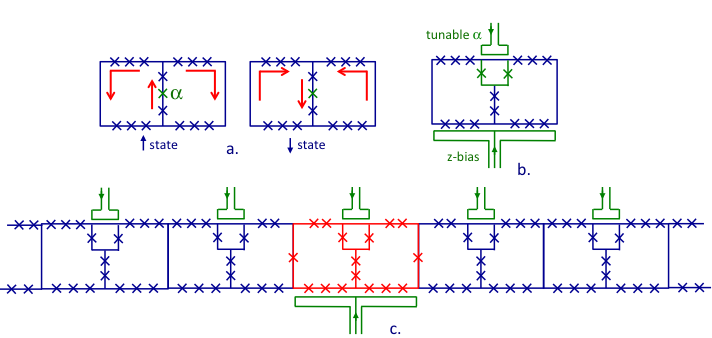
A practical implementation of the proposed schemes can be realised by means of Josephson junction circuits. Flux qubits are particularly suited because a strong coupling between them is easy to achieve and their tunnelling strength, which plays here the role of the transverse field, can be efficiently tuned [14]. A possible circuit is illustrated in Fig. 3. It consists of a chain of gradiometer flux qubits [14]. An individual gradiometer qubit is shown in Fig. 3a. It is an advanced version of the flux qubit [24] (persistent current qubit with a characteristic smaller junction denoted by $\alpha$), in which the outer inductance loop is replaced by two symmetrically placed loops. The two states denoted by $\left|\uparrow\right\rangle$ and $\left|\downarrow\right\rangle$ (eigenstates of $\sigma^{z}$) are the persistent current states depicted in Fig. 3a. The amplitude of tunnelling between $\left|\uparrow\right\rangle$ and $\left|\downarrow\right\rangle$, denoted here by $h$, is controlled by the Josephson energy of the $\alpha$-junction, which can be tuned by replacing it with a two-junction SQUID loop (see Fig. 3b). The gradiometer geometry allows tuning the $\alpha$-junction without affecting the bias energy between $\left|\uparrow\right\rangle$ and $\left|\downarrow\right\rangle$. Typical values could be: qubit tunnelling strength $h=2\pi\hbar\times 1$GHz within the topological region and $h=2\pi\hbar\times 9$GHz outside. The gradiometer inductive loops contain further Josephson junctions; the strength of the nearest-neighbour coupling can be varied by their number. The nearest-neighbour coupling could be $J=2\pi\hbar\times 3$GHz.

The coupler is a special gradiometer qubit with a particularly strong tunnelling, denoted here by $\Delta$ (see Eq. (18)). We envision $\Delta=2\pi\hbar\times 15$GHz. Moreover, an extra magnetic bias ($z$-bias) is needed in order to perform NMR-like rotations of the coupler. This bias can be described by adding to the Hamiltonian a term $H_{z}=-\Omega(t)S^{z}$. The coupling between the coupler and the first qubits of the chains can be made as strong as $v_{1/2}=2\pi\hbar\times 8$GHz (see Eq. (18)). This is achieved by placing extra Josephson junctions into the legs mutual to the coupler and the first qubits (Fig. 3c). These numbers are given as examples, they can be realised with available technology.

Switching of the individual qubits of the chains as well as of the coupler can be effected in a few nanoseconds while the coherence time can be above $10{\rm\mu s}$ [25]. This will allow at least 1000 operations, enough to slide the topological region (5 qubits long) through the coupler and back.

Simulating a controllable Ising-Kitaev chain in the way described above would validate the high level of coherence and control of superconducting flux qubits. This would demonstrate that the superconducting qubits are sufficiently advanced and may simulate fermionic dynamics.

We now ask the following question: Do the protocols developed in this paper for the Ising spin systems provide added insight into the use of topological systems with fermionic Majorana zero modes? First, we mention the recent developments (see Refs. 15, 16) with advanced designs of Majorana wires. Instead of small semiconducting wires placed on top of large superconductors one uses multiple, relatively small elongated superconducting islands placed on top of a semiconducting wire. In Fig. 4 we show a chain of such islands (as described in detail in Refs. 15, 16). It is easy to understand that by allowing for tunnelling between adjacent Majoranas fermions, $H_{T}=i\sum_{n}E_{M}\eta(n)\,\chi(n+1)$, we obtain a system completely equivalent to the Kitaev chain. Here $\eta(n)$ is the right Majorana fermion of island $n$, $\chi(n)$ is the left Majorana fermion of island $n$, and $E_{M}$ is the tunnelling amplitude discussed in detail in Ref. 16. The charging effects are suppressed if the residual Josephson coupling between the islands, $E_{J}$, which is always present in addition to Majorana coupling $E_{M}$ (see Refs. 15, 16), is larger than the charging energy, $E_{C}$ of each island. Alternatively, one can think of coupling the islands to large superconducting reservoirs [15]. The capacitive interactions between the islands do not change the situation qualitatively, as long as they remain small [26].

With the insight gained from the spin representation we envision coupling a flux qubit to one of the links between adjacent sections hosting Majorana fermions as shown in Fig. 5. At this stage we do not discuss the experimental realisation of this setup, which may present a challenge for present-day technology. The idea is to use the phase difference $\varphi$ across the Josephson junction of the qubit (the branch with a single junction) to control the tunnelling of Majoranas. As discussed, e.g., in Ref. 16, the tunnelling Hamiltonian for this particular link reads $H_{T}=iE_{M}\cos(\varphi/2)\eta(n)\,\chi(n+1)$. We consider the situation where the Josephson energy of the flux qubit is much higher than the tunnelling amplitude $E_{M}$. Then the phase difference across the junction can take two well defined values, depending on the quantum state of the flux qubit, and the system of Majoranas has to adjust to these two possible situations. In a usual symmetrically biased flux qubit the phase drop $\varphi$ takes the values $\varphi=\pi\pm\Delta\varphi$ with $\Delta\varphi<\pi/2$. Thus, $\cos(\varphi/2)$ takes one positive and one negative value, and the effective Hamiltonian of the link controlled by the flux qubit becomes $H_{\rm eff}=iJ^{\prime}S^{z}\eta(n)\,\chi(n+1)$, where $J^{\prime}\equiv E_{M}|\cos(\pi/2+\Delta\varphi/2)|$. This Hamiltonian is equivalent to the one considered above for the 1D setup.

In this paper we have proposed setups of Ising spins which allow emulating the physics of Majorana systems and, in particular, performing the braiding operation. In the first case we showed that this is possible in a T-junction geometry, when we introduce an extra spin coupling to the three legs and also appearing as Klein factor in the generalized Jordan-Wigner transformation, thus preserving the proper anticommutation relations. In the second case we showed that a braiding-type protocol can also be performed in a strictly 1D Ising setup, which may be easier to realize in experiments. In addition it allows performing the analogue of parity conserving rotations of a Majorana qubit by an arbitrary angle. This is achieved by placing a special spin-1/2 (coupler) in one of the Ising links of the chain. The coupler controls the sign (ferro- or anti-ferromagnetic) of that Ising link.

This 1D setup emerged in the search for methods to implement (non-protected) topological braiding in Ising chains. The well-known problem is the fact that the Jordan-Wigner transformation, which maps the Ising problem onto the fermionic one, is strictly one-dimensional. Placing a coupler between three Ising chains allows circumventing this obstacle but requires a very special kind of coupling. We showed that the same can be achieved in 1D if one is able to manipulate the coupler between the adiabatic passages of the ferromagnetic (topological) domain through the Ising link controlled by the coupler.

Our protocol could possibly be generalized. One prospective possibility is to rotate the coupler during sliding of the topological (ferromagnetic) domains. This could induce non-trivial Berry phases. Moreover, our protocol can be directly employed in systems containing topologically protected fermionic wires (islands). Such wires would have to be coupled in a non-protected fashion to a spin-1/2 (qubit).

This work was supported by DFG and RSF under RSF grant No. 16-42-01035 and DFG grant No. SH 81/4-1 as well as DFG grant No. SH 81/3-1, DFG CRC183, and the Minerva foundation.

References

- [1] A. Yu. Kitaev. Unpaired Majorana fermions in quantum wires. Physics-Uspekhi, 44(10S):131, 2001.
- [2] Yuval Oreg, Gil Refael, and Felix von Oppen. Helical liquids and Majorana bound states in quantum wires. Phys. Rev. Lett., 105:177002, Oct 2010.
- [3] Chetan Nayak, Steven H. Simon, Ady Stern, Michael Freedman, and Sankar Das Sarma. Non-abelian anyons and topological quantum computation. Rev. Mod. Phys., 80:1083, 2008.
- [4] Jason Alicea, Yuval Oreg, Gil Refael, Felix von Oppen, and Matthew P. A. Fisher. Non-abelian statistics and topological quantum information processing in 1d wire networks. Nature Physics, 7(5):412–417, 05 2011.
- [5] Christina Knapp, Michael Zaletel, Dong E. Liu, Meng Cheng, Parsa Bonderson, and Chetan Nayak. The nature and correction of diabatic errors in anyon braiding. Phys. Rev. X, 6:041003, Oct 2016.
- [6] Torsten Karzig, Yuval Oreg, Gil Refael, and Michael H. Freedman. Universal geometric path to a robust majorana magic gate. Phys. Rev. X, 6:031019, Aug 2016.
- [7] Martin Greiter, Vera Schnells, and Ronny Thomale. The 1d Ising model and the topological phase of the Kitaev chain. Annals of Physics, 351:1026 – 1033, 2014.
- [8] Yaroslav Tserkovnyak and Daniel Loss. Universal quantum computation with ordered spin-chain networks. Phys. Rev. A, 84:032333, Sep 2011.
- [9] A Mezzacapo, J Casanova, L Lamata, and E Solano. Topological qubits with majorana fermions in trapped ions. New Journal of Physics, 15(3):033005, 2013.
- [10] Jin-Shi Xu, Kai Sun, Yong-Jian Han, Chuan-Feng Li, Jiannis K. Pachos, and Guang-Can Guo. Simulating the exchange of Majorana zero modes with a photonic system. Nature Communications, 7:13194 EP –, 10 2016.
- [11] Jin-Shi Xu, Kai Sun, Jiannis K. Pachos, Yong-Jian Han, Chuan-Feng Li, and Guang-Can Guo. Experimental simulation of Majorana-based quantum computation. arXiv:1702.08407, 2017.
- [12] L. S. Levitov, T. P. Orlando, J. B. Majer, and J. E. Mooij. Quantum spin chains and Majorana states in arrays of coupled qubits. cond-mat/0108266, 2001.
- [13] B. van Heck, A. R. Akhmerov, F. Hassler, M. Burrello, and C. W. J. Beenakker. Coulomb-assisted braiding of Majorana fermions in a Josephson junction array. New Journal of Physics, 14(3):035019, 2012.
- [14] F. G. Paauw, A. Fedorov, C. J. P. M Harmans, and J. E. Mooij. Tuning the gap of a superconducting flux qubit. Phys. Rev. Lett., 102:090501, Mar 2009.
- [15] David Aasen, Michael Hell, Ryan V. Mishmash, Andrew Higginbotham, Jeroen Danon, Martin Leijnse, Thomas S. Jespersen, Joshua A. Folk, Charles M. Marcus, Karsten Flensberg, and Jason Alicea. Milestones toward Majorana-based quantum computing. Phys. Rev. X, 6:031016, Aug 2016.
- [16] Michael Hell, Jeroen Danon, Karsten Flensberg, and Martin Leijnse. Time scales for Majorana manipulation using Coulomb blockade in gate-controlled superconducting nanowires. Phys. Rev. B, 94:035424, Jul 2016.
- [17] Pierre Pfeuty. The one-dimensional Ising model with a transverse field. Annals of Physics, 57(1):79 – 90, 1970.
- [18] Boris Narozhny. Majorana fermions in the nonuniform Ising-Kitaev chain: exact solution. Scientific Reports, 7(1):1447, 2017.
- [19] U. Dorner, P. Fedichev, D. Jaksch, M. Lewenstein, and P. Zoller. Entangling strings of neutral atoms in 1d atomic pipeline structures. Phys. Rev. Lett., 91:073601, Aug 2003.
- [20] J. Q. You, Z. D. Wang, Wenxian Zhang, and Franco Nori. Encoding a qubit with Majorana modes in superconducting circuits. Scientific Reports, 4:5535 EP –, 07 2014.
- [21] N. Crampé and A. Trombettoni. Quantum spins on star graphs and the Kondo model. Nucl. Phys. B, 871(3):526–538, 2013.
- [22] A. M. Tsvelik. Majorana fermion realization of a two-channel Kondo effect in a junction of three quantum Ising chains. Phys. Rev. Lett., 110:147202, Apr 2013.
- [23] M. Pino, A. M. Tsvelik, and L. B. Ioffe. Unpaired Majorana modes in Josephson-junction arrays with gapless bulk excitations. Phys. Rev. Lett., 115:197001, Nov 2015.
- [24] J. E. Mooij, T. P. Orlando, L. Levitov, Lin Tian, Caspar H. van der Wal, and Seth Lloyd. Josephson persistent-current qubit. Science, 285(5430):1036–1039, 1999.
- [25] Fei Yan, Simon Gustavsson, Archana Kamal, Jeffrey Birenbaum, Adam P Sears, David Hover, Ted J. Gudmundsen, Danna Rosenberg, Gabriel Samach, S Weber, Jonilyn L. Yoder, Terry P. Orlando, John Clarke, Andrew J. Kerman, and William D. Oliver. The flux qubit revisited to enhance coherence and reproducibility. Nature Communications, 7:12964, 11 2016.
- [26] Suhas Gangadharaiah, Bernd Braunecker, Pascal Simon, and Daniel Loss. Majorana edge states in interacting one-dimensional systems. Phys. Rev. Lett., 107:036801, Jul 2011.