2017 March 21st
Warped in Type IIB supergravity II
Global solutions and five-brane webs
Eric D’Hoker, Michael Gutperle and Christoph F. Uhlemann
Mani L. Bhaumik Institute for Theoretical Physics
Department of Physics and Astronomy
University of California, Los Angeles, CA 90095, USA
dhoker@physics.ucla.edu; gutperle@ucla.edu; uhlemann@physics.ucla.edu
Abstract
Motivated by the construction of holographic duals to five-dimensional superconformal quantum field theories, we obtain global solutions to Type IIB supergravity invariant under the superalgebra on a space-time of the form warped over a two-dimensional Riemann surface . In earlier work, the general local solutions were expressed in terms of two locally holomorphic functions on and global solutions were sketched when is a disk. In the present paper, the physical regularity conditions on the supergravity fields required for global solutions are implemented on for arbitrary . Global solutions exist only when has a non-empty boundary . The differentials are allowed to have poles only on and each pole corresponds to a semi-infinite five-brane. The construction for the disk is carried out in detail and the conditions for the existence of global solutions are articulated for surfaces with more than one boundary and higher genus.
1 Introduction
In a recent paper [1], we solved the BPS equations of Type IIB supergravity for configurations with 16 residual supersymmetries on a space-time of the form warped over a Riemann surface . The isometry algebra of this space-time is uniquely completed into the exceptional Lie superalgebra with 16 fermionic generators [2, 3]. In the present paper we shall impose on the local solutions of [1] the positivity and regularity conditions needed to obtain physically sensible supergravity fields and we shall construct the corresponding general global solutions. The first part of the present paper provides detailed derivations and discussions of results which were described in a short note [4].
The motivation for this work stems from the study of five-dimensional supersymmetric quantum field theories with the help of holographic methods. Minimal Poincaré supersymmetry in five dimensions has eight supersymmetry generators and R-symmetry. In their conformal phase, five-dimensional supersymmetric field theories will have conformal symmetry, R-symmetry and sixteen supersymmetries and therefore be invariant under the superconformal algebra. Unlike in space-time dimensions three, four, and six, where the maximal superconformal algebra has thirty two supersymmetries, in five dimensions the superconformal algebra is unique and has sixteen supersymmetries.
The existence of physically consistent interacting five-dimensional gauge theories is far from obvious since standard perturbative methods show them to be non-renormalizable. Arguments for the existence of non-Abelian gauge theories were advanced in [5] and in [6] and drew heavily on the structure imposed by five-dimensional Poincaré supersymmetry and the dynamics on the Coulomb branch. It was further argued that the theory in the non-conformal Coulomb phase can flow to a strongly coupled fixed point with superconformal symmetry. The five-dimensional gauge theories of [5, 6] can have gauge groups or for arbitrary , as well as exceptional gauge groups. Consequently, one should expect that, in the large limit, the theories with gauge groups and will admit weakly coupled gravity duals. The explicit construction of such gravity duals is the goal of [1] as well as of the present paper.
Several brane realizations of five-dimensional gauge theories with eight Poincaré supersymmetries have appeared in the string theory literature. In [5, 7, 8] Type IIA supergravity solutions were constructed using D4-branes near a stack of D8/O8 branes. These solutions suffer from singularities associated with the presence of the D8/O8 branes.
In [9, 10, 11] a large class of five-dimensional theories was constructed in Type IIB string theory using brane webs. The five-dimensional field theories live on D5 branes which are of finite extent in one dimension and are embedded in a web of semi-infinite five-branes as well as optional seven-branes. The brane webs realize the moduli space and the matter content of such theories geometrically, generalizing the construction of three-dimensional theories [12] to five dimensions.
The solutions constructed in [1] are local in the sense that all BPS conditions, Bianchi identities and field equations are satisfied point-wise by the choice of two locally holomorphic functions on a two-dimensional Riemann surface whose global structure is as yet undetermined.11 1 Previous attempts to construct warped solutions have appeared in [13, 14, 15], but the partial differential equations derived from the BPS conditions have remained unsolved in these papers. In [1], we followed the strategy developed some time ago in [16, 17, 18], and utilized the integrable structure of the reduced BPS equations [19] along with the holomorphic structure of the Riemann surface to its fullest. These techniques have generated the complete local solution to the BPS equations.
The local solutions of [1] need to be supplemented by positivity and regularity conditions in order to produce genuine global supergravity solutions with physically sensible behavior of all supergravity fields. These positivity and regularity conditions are as follows. First, all supergravity fields must satisfy the reality conditions appropriate for Type IIB, such as for example the space-time metric and the dilaton field must be real. Second, the space-time metric must have the correct ten-dimensional Minkowski signature. Third, the space-time metric must be geodesically complete. Fourth, any singularities that might occur in the solutions, such as curvature singularities or a divergent string coupling, must be associated with physically sensible sources, such as BPS branes already present in Type IIB.
The main new result of the present paper is the complete construction of global solutions which satisfy all the positivity and physical regularity conditions enumerated above. Our solutions evade a recently obtained theorem [20] stating that no supersymmetric warped solutions exist in Type IIB supergravity, since our solutions are warped over a non-compact Riemann surface which violates one of the assumptions of the no-go theorem of [20]. We shall show that the resulting global solutions provide viable candidates for holographic duals to five-dimensional superconformal field theories in the large- limit.
The organization of this paper is as follows. In section 2, we present a brief review of the local supergravity solutions in terms of holomorphic functions obtained in [1]. We articulate the positivity and regularity conditions in quantitative terms, formulate our strategy for the construction of global solutions, and show that no physically sensible solutions exist unless has a non-empty boundary. In section 3, we present a new class of global solutions for which the Riemann surface is the upper half plane and which are parameterized by holomorphic functions with simple poles on the boundary of . For these general solutions we provide a detailed counting of the number of free moduli of the space of solutions. In section 4 we present explicit examples with three and four poles and discuss natural connections to 5-brane webs. In section 5 we extend the general construction to the case where is an annulus, and in section 6 to the case where has arbitrary genus and an arbitrary non-zero number of boundary components. In the case of more than one boundary component some global regularity conditions remain to be imposed on the solutions. Finally, in section 7, we conclude with a discussion of our results and present some directions for future research.
2 Local solutions and strategy for global solutions
In this section, we begin by summarizing from [1] the structure of the local solutions to the BPS equations in Type IIB supergravity with 16 supersymmetries and isometry on a space-time of the form warped over a Riemann surface . We then review the reality and positivity conditions required on the physical supergravity fields, and impose mild regularity conditions. Finally, we discuss our strategy for the construction of global solutions starting from an analogy with two-dimensional electrostatics.
2.1 Supergravity fields in terms of holomorphic functions
The isometry dictates the Ansatz for the bosonic supergravity fields, while the fermionic fields vanish. The five-form field strength vanishes by symmetry, while the metric and the complex three-form flux fields are as follows,
| (2.1) |
Here, , and the dilaton-axion scalar field are functions of only. The metrics and are the and invariant metrics with unit radius respectively on and , and is the corresponding volume form on . Finally, we have introduced local complex coordinates in terms of which the metric on is conformally flat.
The supergravity fields for the local solutions were obtained in [1], and expressed in terms of locally holomorphic functions on the Riemann surface . Of fundamental importance to the structure of the local solutions and, as we shall see shortly also to the structure of the global solutions, are the following real functions, (more properly, one should think of as a differential on ),
| (2.2) |
where the locally holomorphic function is defined up to an additive constant by the relation,
| (2.3) |
In Einstein frame, the metric functions , and are given by,
| (2.4) |
where the real positive function is defined by the following quadratic equation,
| (2.5) |
The axion-dilaton field is given by,
| (2.6) |
while the flux potential function for the three-form field strength takes the form,
| (2.7) |
Residual gauge transformations, which act on by a constant shift, leave invariant. The constant can be absorbed into a rescaling of and we will therefore set it to one in the following.
2.2 symmetry and monodromy
Under the symmetry of Type IIB supergravity, the metric in the Einstein frame and the five-form field strength are invariant while the axion-dilaton field and the three-form field strength transform non-trivially. Upon reduction to the Ansatz, the metric factors are invariant under , the five-form field strength is zero which is -invariant, while and transform as follows,
| (2.8) |
where the additive constant in allows for a gauge transformation.
Correspondingly, the building blocks and of the metric factors must be invariant under . The invariance of combined with the transformation rule of dictate the transformation rule for the differentials ,
| (2.9) |
Integration of the differentials and gives the transformation rule of and ,
| (2.10) |
where and are complex constants. The function is invariant provided we impose,
| (2.11) |
The combined transformations on form a group , whose action on the differentials reduces to the action of the subgroup .
When has a non-trivial fundamental group the functions are allowed to have -valued monodromy around non-trivial closed loops on . The monodromy on the differentials is simplest and given by a representation of . Mathematically, this representation could be arbitrary. Physically, for a supergravity embedded into Type IIB string theory, however, the monodromies generated by parabolic elements acting on the axion field by a shift correspond to the presence of D7 branes, and have a well-known interpretation. It is also possible for the differentials to have a branch point in the interior of around which axion monodromy is allowed.
In the present paper, we shall consider solutions only for which the dilaton/axion field is single-valued and no D7 branes are present. We plan to investigate solutions with nontrivial monodromies in the future.
2.3 Positivity, regularity and boundary conditions
Reality and positivity of the function in (2.5) require and to have the same sign. Reality of and positivity of the metric factors require to have the same sign as . Without loss of generality, we may choose the branch in (2.5) resulting in the following positivity conditions in the interior of the Riemann surface ,
| (2.12) |
These necessary conditions are sufficient to guarantee that are real and positive.
The topology of , namely its genus and number of its boundary components, remains to be determined by global considerations. The boundary of the surface does not correspond to a boundary of the physical space-time manifold of the supergravity solution. Instead, corresponds to the shrinking of as part of the slicing of a regular cycle, thereby ensuring the geodesic completeness of the full space-time geometry. As such, we may characterize by and or, equivalently, by the following conditions,
| (2.13) |
We shall now prove the following Proposition,
- 1.
There are no regular solutions satisfying (2.12) when is compact without boundary.
- 2.
For an arbitrary Riemann surface , with non-empty boundary , the condition implies everywhere in the interior of provided .
A practical implication of this proposition is that it will suffice to establish the property on in order to guarantee the condition of (2.12) in the interior of .
To prove the Proposition we begin by evaluating the mixed derivative of in the second line of (2.2) in terms of with the help of the first line of (2.2),
| (2.14) |
To prove item 1 of the Proposition, we assume that is compact without boundary and that and are sufficiently regular. Integrating both sides of (2.14) over , the left side vanishes since has no boundary, yet the right side must be strictly negative since in the interior of . Therefore, (2.14) has no solutions consistent with the requirements of (2.12). This statement is in agreement with results found in a recent paper [20] stating that there are no supersymmetric solutions which are warped over a compact space.
To prove item 2 of the Proposition, we solve equation (2.14) along with the boundary condition on in (2.13) to obtain the following integral equation,22 2 Throughout, we shall use the following normalizations and .
| (2.15) |
Here, is the scalar Green function on , which is symmetric and vanishes on the boundary ,
| (2.16) |
For any two points in the interior of , the function is strictly positive, as we shall review below, and therefore in view of in the interior of .
To prove positivity of the Green function for arbitrary points in the interior of , we fix and define to be the Riemann surface minus the disk of radius centered at the point . In the interior of the function is real harmonic in the variable . By the minimum-maximum principle for harmonic functions, takes its minimum and maximum values on the boundary of . Since vanishes on by (2.13) and, for sufficiently small is positive on the circle of radius centered at , it follows that must be strictly positive in the interior of and thus in the interior of as we take the limit .
2.4 Strategy for global solutions without monodromy
The construction of global supergravity solutions has now been reduced to solving for two locally holomorphic functions on a Riemann surface with non-empty boundary , subject to the positivity condition in the interior of of (2.12) and the boundary conditions on . The positivity condition in the interior of in (2.12) is then automatic by the Proposition of the preceding subsection. In the present subsection, we shall present our general strategy for solving these conditions, with the assumption that the differentials are meromorphic on , and in the absence of monodromy.
We fix a Riemann surface with non-empty boundary . We shall use an analogy with two-dimensional electrostatics to solve for the meromorphic differentials . We begin by introducing the meromorphic function on ,
| (2.17) |
Our strategy will consist of the following steps,
- 1.
solving for the function using the properties of and an electrostatics analogy;
- 2.
constructing the meromorphic differentials and their integrals ;
- 3.
enforcing the condition on the boundary of .
2.4.1 Constructing the function via an electrostatics analogy
We begin by constructing the meromorphic function . The further properties of follow from its definition (2.17) and the properties of in (2.12) and (2.13), and we have,
- •
in the interior of in view of ;
- •
on the boundary of in view of on ;
- •
is holomorphic in , since it is meromorphic and bounded in .
To solve for subject to these properties, we use an electrostatics analogy. We view the function as an electrostatic potential for an array of point-like charges. This potential is real, and the properties of imply that is locally harmonic, strictly positive in the interior of , and zero on the boundary . The potential must have singularities, since otherwise it would vanish throughout. Its singularities are located at the zeros of in the interior of and are logarithmic. Combining these results, we find,
| (2.18) |
where is the scalar Green function defined in (2.16). The charges are real and strictly positive for all . Since we have on , the points must lie in the interior of , away from the boundary.
Conversely, when the charges are all positive, the potential constructed in (2.18) is positive throughout the interior of . This result may be established by using the positivity of the scalar Green function , already proven at the end of subsection 2.3. To construct a single-valued from (2.18) further requires the charges to be integers. The holomorphic function may be obtained by holomorphically splitting (2.18), and the result is unique up to an arbitrary phase factor. The precise expressions will be given in the sequel when is the upper half plane, an annulus, or a Riemann surface of higher genus.
2.4.2 Constructing the differentials
To construct the differentials we decompose into a ratio of holomorphic functions (or holomorphic differentials of equal weight) ,
| (2.19) |
The functions are clearly not unique, but we may impose the irreducibility condition that has no zeros in the interior of or on its boundary. In that case, the zeros of coincide with the zeros of and are given by the points of (2.18). Choosing local complex coordinates near a given boundary component in which the boundary is represented by a segment of the real line, we require to obey the following conjugation property,
| (2.20) |
which guarantees the relation when is real and on the boundary of . The meromorphic differentials are then given as follows,
| (2.21) |
where is a meromorphic function or differential on .
The properties of , and narrow down the properties of . The combinations must be single-valued meromorphic 1-forms on . The form can have neither zeros nor poles in the interior of , since a zero would make vanish in contradiction with (2.12), and a pole would produce local monodromy in the supergravity fields. Thus, the zeros and poles of must all lie on , so that is an imaginary function satisfying in local complex coordinates where the local boundary corresponds to real . Therefore we have the following conjugation property for the meromorphic differentials ,
| (2.22) |
On an arbitrary Riemann surface , with non-empty boundary , the conjugation condition may be formulated globally in terms of the double surface , equipped with an anti-conformal involution , such that , and each point on the boundary is mapped to itself under . This formalism will be developed and used to construct in section 6.
2.4.3 Enforcing the condition on
To analyze the vanishing of on , we locally integrate the conditions (2.22). By choosing the integration constants, we may impose the following conjugation property,
| (2.23) |
While the differentials are meromorphic and have poles on , their integrals will have logarithmic branch points on whose branch cuts must be chosen consistently with the conjugation condition (2.23).
The condition (2.22) suffices to guarantee that is constant along any line segment of an arbitrary boundary component which is free of poles in . To prove this statement, we consider the derivative tangent to the boundary component of the real function . Since here we have parametrized the boundary component locally by the real part of we find, using (2.2) and (2.22),
| (2.24) | |||||
Along a boundary component away from poles in , the variable is real and the differences of the derivative terms vanish identically. Therefore vanishes and is constant on any such segment of an arbitrary boundary component. To promote the piecewise constancy of to the vanishing of throughout the boundary will require restrictions on the free parameters of the functions . We shall establish later that there will be one real condition for each pole. When has several disconnected boundary components, there will be further conditions to ensure that along each boundary component separately.
3 Global solutions for the upper half plane
In this section, we shall construct explicitly the global solutions for which has genus zero and a single boundary component. In this case may be mapped to the unit disk whose boundary is the unit circle, or to the upper half complex plane whose boundary is the real axis. Our construction will follow closely the strategy outlined in section 2.4, and it will be convenient to identify with the upper half plane and .
3.1 The function
The starting point is the general formula for given in (2.18), for an array of positive integer charges located at points in the upper half plane with . Without loss of generality, we set for all and obtain higher integer charges by coalescing charges at different points if need be. The set-up is represented schematically in Figure 1. The scalar Green function for is given by,
| (3.1) |
The resulting formula for is,
| (3.2) |
Here, is an arbitrary phase factor, which may be viewed as effecting an transformation and on the solution with . Following the process leading to (2.19), we express the function , which is holomorphic on and meromorphic in , as the ratio of functions which are both holomorphic in , and which are complex conjugate functions of one another,
| (3.3) |
The irreducible solution for , in the sense of subsection 2.4.2, is unique and given by,
| (3.4) |
We note that has a smooth limit as any one of its complex zeros approaches the real line, , so that the condition could actually be smoothly relaxed to , with the understanding that at least one of the zeros must satisfy .
3.2 The differentials
The holomorphic functions and the meromorphic differentials satisfy the relation,
| (3.5) |
Eliminating between this relation and its complex conjugate relation obtained from (3.3), requires the doublet of differentials to be proportional to the doublet of differentials by a meromorphic function we shall denote . Involution of the complex conjugation operation then imposes a conjugation condition on , given as follows,
| (3.6) |
To construct the differentials we analyze the zeros on both sides of (3.5). Since has no zeros in the upper half plane, the set of zeros of is the union of the set of zeros of and the set of zeros of (counted with multiplicities). But if the differentials have a common zero, then must vanish there. Strict positivity of in the interior of prohibits such zeros. Thus, any zero common to must be on the real line.
All poles must be common to since their ratio is bounded in the upper half plane. A simple pole in the interior of the upper half plane will produce a logarithmic branch cut in . In appendix A we give an argument that no such poles occur and, by complex conjugation, that no poles occur in the lower half plane as well. Thus, all poles in must be common and on the real axis. We shall denote the positions of the poles by with , for an as yet undetermined number .
Putting all together, we find the following general expression for the differentials ,
| (3.7) |
The zeros satisfy for all with at least one zero having strictly positive imaginary part; the poles are real for all ; and the constant is complex. Regularity of the differentials at imposes the condition as , which provides us with a relation between and , given by,
| (3.8) |
The function of (3.6) is then a constant phase, given by . In summary, the differentials given in (3.7) automatically satisfy in the interior of and on . It remains to enforce the condition on . To compute , we need and which we compute in the subsequent subsections.
3.3 The functions
The functions may be obtained from the meromorphic differentials by integration. Performing this integration is greatly facilitated by expressing the meromorphic differentials of (3.7) in terms of their partial fraction decomposition with residues ,
| (3.9) |
The residues may be read off from the product formulas (3.7) and are given by,
| (3.10) |
Since must have at least one zero in the upper half plane we have and the number of poles satisfies . We now integrate the differentials to get , as follows,
| (3.11) |
where are two complex integration constants. Throughout, we shall choose the branch cuts of the logarithm so that is real for real and positive, and use the following continuation formula by circling the branch point in the upper half plane,
| (3.12) |
As a result, the functions have monodromy around each pole , whose value is given by . In view of the third equation in (3.9), there is no monodromy at , consistent with treating infinity as a regular point.
3.4 The functions and
Using (3.9) and (3.11), we integrate the definition for given in (2.3),
| (3.13) |
where is an arbitrary complex integration constant, is an arbitrary reference point, and we have introduced the following convenient abbreviation,
| (3.14) |
A change in in (3.13) may be compensated by a change in , so that the parametrization provided above is subject to a redundancy which will be conveniently fixed shortly. Substituting the expressions for , , , and into the formula for given in (2.2), we obtain the following expression,
| (3.15) | |||||
where is a real constant given by,
| (3.16) |
A change in will shift . The constants , and , as well as the positions of the zeros and the poles remain undetermined at this stage. The integrals are related to dilogarithms, and cannot be evaluated in terms of elementary functions.
3.5 Necessary conditions for vanishing on
We shall now enforce the condition on the boundary , and derive the corresponding conditions on the zeros , poles and other parameters of the solution. Since the integrals on the last line of (3.15) are related to dilogarithms in , the function can vanish for all only provided the contribution of the dilogarithms vanishes by itself. This requires , given the branch cut choice we have made. Since is then real, the contribution of the second line in (3.15) vanishes for since the combination is anti-symmetric in , while the logarithmic factor becomes symmetric in for real . Cancellation of the terms on the first line of (3.15) for any further requires,
| (3.17) |
The conjugation conditions on the residues then reads as follows for all ,
| (3.18) |
and the combinations are imaginary-valued. We shall require the following relation between the integration constants,
| (3.19) |
Indeed, we may do so without loss of generality since the only supergravity field that involves the combinations is the flux field , and the condition (3.19) simply amounts to a (constant) gauge choice for . Having imposed (3.19) we see that the above conditions on precisely imply the conjugation relations of (2.23) advocated on general grounds.
3.6 Sufficient conditions for vanishing on
Due to the presence of branch points in on the real axis, the above conditions are necessary but not sufficient, however, as the monodromy makes the value of jump across the branch points. To impose the further condition that has zero discontinuity on the real axis across a pole , we proceed as follows. Having chosen the branch cuts such that is real for real and positive, we may order the real poles for as follows,
| (3.20) |
We shall choose the arbitrary reference point to be real with . We then have for real and provided we set .
We make the convergence of the combined integrals in (3.15) as explicit by anti-symmetrizing in , and letting . The only dependence of the resulting formula for on the integration constants is through the combination . The resulting expression for is given by,
| (3.21) | |||||
To derive the discontinuity of across a pole we evaluate the function as approaches any point in the open interval from above. To do so, it will be convenient to partition the sums over according to their position with respect to . The integrals do not contribute for the partition since the logarithms are manifestly real there. We evaluate the remaining integrals as a function of the position of on the real axis with respect to the points , and , using the contours of Figure 2. The integral evaluated with the help of contour (a) of Figure 2 for in the open interval is given by,
| (3.22) |
The integral evaluated with the help of contour (b) of Figure 2 for in the open interval is given by,
| (3.23) |
Substituting the evaluated integrals into the formula for , we obtain after the straightforward cancellation of all -dependence,
| (3.24) |
valid for . Retaining the above condition for unchanged, and subtracting from the condition for the condition obtained by letting , we obtain a total of conditions, expressed below for ,
| (3.25) |
Both terms are purely imaginary in view of the conjugation property (3.18) and the definition (3.14). Only of these conditions are linearly independent since the sum over all of the above conditions vanishes by anti-symmetry in of the pre-factor .
We also note that the final form of the conditions does not depend on a particular ordering of the poles on the real axis. Subtracting the condition localizes the calculation around the pole and, while convenient for the derivation of the conditions, the assumption on the ordering can be safely relaxed in (3.25).
We close this subsection with the explicit expression for which vanishes on the boundary (away from the poles). Using (3.25) to eliminate in (3.21) converts the first line in (3.21) to a double sum similar to the remaining terms. Anti-symmetrizing in , yields,
| (3.26) |
where the complex conjugation applies to the entire expression inside the bracket. Note that is real in view of the fact that is purely imaginary.
3.7 acting on
acting on transforms and as follows with and . The differentials in (3.7) and the functions in (3.11) are invariant under provided the data transform as follows,
| (3.27) |
The residues in (3.9) are then invariant, as are the conditions of (3.25). The -invariance therefore allows us to fix the positions of three of the poles at will.
3.8 Counting free parameters
We label the families of solutions by a positive integer which is the number of zeros of in the upper half plane. The independent parameters of the solutions constructed in section 3 are then given by,
| (3.28) |
Note that, even though and are complex, they satisfy and which accounts for them representing only one real parameter each. Furthermore, of the two complex constants , only the combination enters into the metric factors and the dilaton-axion field, while in the flux potential, the combination produces merely a gauge transformation of . Therefore, of the constants only is a genuine physical parameter. Finally, in counting the number of poles , we have made use of the relation of (3.8) which relates the number of poles to the number of zeros. The total number of parameters is thus .
The parameters of (3.28) must satisfy the regularity relations obtained in (3.25), which reduces the number of free parameters by . Furthermore, the automorphism group of the upper half plane maps to physically equivalent solutions and therefore further reduces the number of free physical parameters by 3. As a result the number of moduli of the global solutions is given by,
| (3.29) |
3.9 Asymptotic behavior near the poles
The global solutions we have constructed above are regular everywhere in the interior of , and on the boundary of away from the poles . In this subsection, we shall derive the asymptotic behavior of the supergravity fields near the poles , and then provide a physical interpretation of this behavior in terms of five-brane webs. The original Ansatz and solutions were formulated in Einstein frame metric, where symmetry is manifest, and we shall begin by obtaining the asymptotics in this frame. Subsequently to make contact with brane behavior, we shall translate the asymptotics to the string frame.
3.9.1 Asymptotic behavior near the poles in Einstein frame
We will use the expressions for the Einstein frame metric factors in terms of the function , its derivatives, and the functions and given in (2.4). To do so, we derive first the asymptotic behavior of and near a pole , and parametrize the coordinate near a pole as follows,
| (3.30) |
where and for all . The expansion of near in terms of the parametrization by is then given by,
| (3.31) |
which implies that the asymptotic expansion of is given by,
| (3.32) |
The coefficients are real in view of the fact that for and , and may be taken to be positive.
To calculate the asymptotic form of we use (3.26). To exhibit the asymptotics of the integral near the pole we use the fact that vanishes on the real line away from the pole and choose the point where to write and thus,
| (3.33) | |||||
The leading contributions are from the terms in the sum where either or . Since the entire contour for the integral is close to the pole, we can then expand the integrand appropriately, and find,
| (3.34) |
The leading behavior of the metric functions near the pole is given by,
| (3.35) |
The dilaton and axion fields are obtained from (2.6) with
| (3.36) |
To leading order, as , and are given by,
| (3.37) |
Clearly, the dilaton diverges at the pole provided .
3.9.2 Asymptotic behavior near the poles in string frame
Since the dilaton diverges near the poles, there is a qualitative difference in behavior between the metric in the Einstein frame (where duality is manifest) and the metric in the string frame (where the connection with D-branes is transparent). We shall denote the metric factors in the string frame by and . Their relation with the metric factors of the Einstein frame, and their asymptotic behavior near the pole are given by,
| (3.38) |
Converting the metric in the Einstein frame of the Ansatz of (2.1) to the metric in the string frame, and using the relation , the near-pole metric in string frame becomes,
| (3.39) |
The last two terms combine into the round metric of a smooth sphere. This produces a regular geometry in string frame. The curvature radius of the part diverges as the pole is approached, which turns it into a six-dimensional Minkowski space.33 3 To see this more explicitly, say we start with the Poincaré patch and . Setting and yields, up to terms which are subleading in the near-pole limit, , and we indeed recover flat space. Since flat space does not have an intrinsic scale, we can absorb overall constants into a rescaling of the coordinates and find the near-pole string-frame metric,
| (3.40) |
It is important to note that while our supergravity solutions are singular at the poles , we shall argue in the discussion below that these singularities have a clear and compelling physical interpretation in terms five-branes. This is to be contrasted with previously constructed Type IIB solutions [13, 14, 15].
3.9.3 Asymptotic behavior of the flux form near the poles
Finally, the shift in the flux potential , as the pole at is being circumnavigated in the upper half plane from the right to the left, namely from to , is determined by examining (2.7). The variables , , and do not shift. The shift in cancels, and with we find the shift in ,
| (3.41) |
This expression is exact. Evaluating the asymptotic behavior of the flux potential itself we find,
| (3.42) |
As , is regular and the leading neglected term vanishes. Finally, the factor gives the volume form of the S3 sphere in (3.40). Integrating (3.42) from to reproduces (3.41).
3.10 Identification of the poles with 5-branes
With the asymptotic behavior of the solution and the shift in the flux potential around the poles in hand, we can now give a physical interpretation of the poles. To this end we compare the near-pole behavior to the well-known supergravity solution for a 5-brane as given in [21]. With the string-frame metric (3.40), axion and dilaton (3.37) and complex three-form field strength (3.42), we find an exact correspondence with the geometry near a 5-brane, with matching axion, dilaton, and 3-form field strength. More precisely, matching the 3-form field strength given above with the results presented in [21] and denoting and yields the identification,
| (3.43) |
The near-pole behavior of our global solutions then matches the near-brane behavior of the 5-brane solution not only in scaling and functional form of the various fields and involved geometry, but also in the overall coefficients.44 4 For an explicit match, the radial coordinate of [21] should be identified with used here as . The leading-order expansion of (22), (23) (24) of [21] near the 5-brane then matches the expansions of the corresponding quantities near the poles derived in sec. 3.9. The complex 3-form field strength is related to the real , of [21] by . This demonstrates that the poles in our solutions correspond to external 5-branes as they typically appear in the brane web diagrams. As we have already advocated briefly in [4], this evidence strongly suggests that the solutions correspond to fully localized intersections of 5-branes.
4 Example solutions and relation to 5-brane webs
In this section we provide explicit realizations and corresponding numerical plots for the solutions on the upper half plane in the case where the number of poles is three and four. These numerical results are used to illustrate the validity of the general regularity arguments made in the previous sections and to provide explicit physically acceptable supergravity solutions. In addition, we confirm the claim, briefly advocated already in [4] and discussed in greater detail in the present paper, that the general -pole solutions for the upper half plane can be identified precisely with fully localized intersections of 5-branes. We show that the corresponding features discussed in the previous sections indeed admit a natural interpretation as properties of the intersection. In 4.3 we shall extend this discussion and speculate on how the solutions relate to 5-brane webs and the corresponding SCFTs.
4.1 Solutions with three poles
In this subsection, we discuss the family of minimal solutions with zeros and poles in the differentials . It follows from the counting given in (3.29) that this family of solutions has four real free parameters. Using the automorphism group of the upper half plane, we may choose the poles to reside at . As argued in the previous section, the single zero must lie strictly in the upper half plane,
| (4.1) |
The four real parameters are the complex zero and the overall complex normalization . The residues are calculated from (3.10), and we obtain,
| (4.2) |
the residues being given by for . We then have,
| (4.3) |
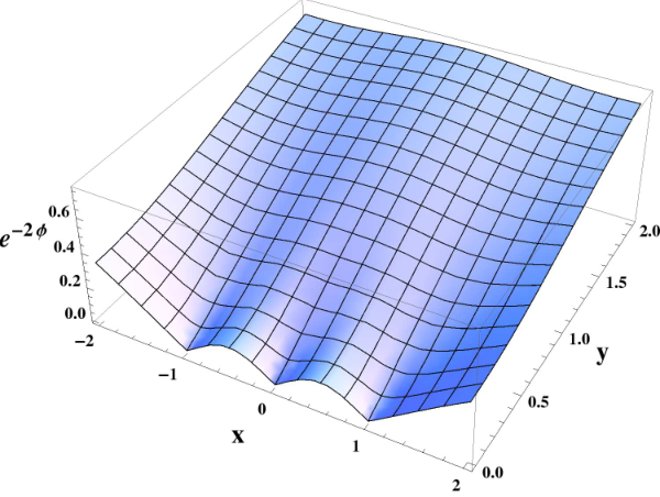
and the relations (3.25) are solved by . The metric functions, dilaton/axion fields and flux potential all involve polylogarithms and do not admit a simple form. Therefore, we shall directly resort to a numerical evaluation of the supergravity fields of the solution. In Figure 3 we illustrate the behavior of the metric functions in the Einstein frame, as well as the axion, dilaton and the two-form potential for the following choice of the four free parameters,
| (4.4) |
For stable numerical evaluation we note that, since assumes a maximum in the interior of and at that point, the expression for in (2.4) has to be treated with care. The expression is regular since when , and to make the regularity of explicit we rewrite it in a manifestly regular form. This leads to the following exact alternative expressions for the metric factors,
| (4.5) |
They were derived directly from (2.4) and we have therefore included the appropriate powers of . The plots show that the exponentiated dilaton is positive, as required, and goes to zero at the poles, as derived in sec. 3.9. The metric factors are real and positive, as desired, and behave at the poles precisely as discussed for the Einstein frame in sec. 3.9. At the boundary of , vanishes as required to have a smooth ten-dimensional geometry without boundary, and stays finite except for at the poles. The two-form potential is piecewise constant at the boundary, and jumps at the poles in accordance with (3.41). Moreover, it approaches the same value to the left and to the right of all poles, reflecting charge conservation.
 |
 |
 |
|
 |
 |
 |
 |
4.2 Solutions with four poles
Solutions with four poles have six real free parameters. We use invariance to fix the positions of three of the four poles on the real line. We may choose the remaining free parameters to be the two complex zeros and one complex overall normalization, with and the position of the fourth pole determined from (3.25). A more physically motivated choice of parameters is as follows. Via the identification in sec. 3.10, the poles correspond to four stacks of semi-infinite external 5-branes, and the residues are related to their charges. Alternatively, we may choose three complex residues at three of the poles as the free parameters, the residue at the fourth pole then being determined by the condition that the sum of the four residues vanishes in (3.9). We will look at the special family of solutions where the residues are related as follows,
| (4.6) |
That is, the stacks of semi-infinite external 5-branes have pairwise opposite charges. Due to the relation the two relations above are equivalent to one another. Using to fix the position of three poles as follows,
| (4.7) |
the position of the remaining pole, remains a free parameter. The conditions (4.6) and (3.25) are solved by,
| (4.8) |
Since the relation between and is an transformation, both will be in the upper half plane provided either one is. The resulting charges are,
| (4.9) |
with and given by (4.6).
 |
 |
 |
|
 |
 |
 |
 |
We will take a closer look at the particular solutions obtained by choosing
| (4.10) |
For the imaginary part is positive for both zeros and , corresponding to the location of the charges in the electrostatics analogy. They are interchanged upon changing the branch of the square root and become coincident for . The residues, fixing the charges of the external 5-branes via (3.43), are
| (4.11) |
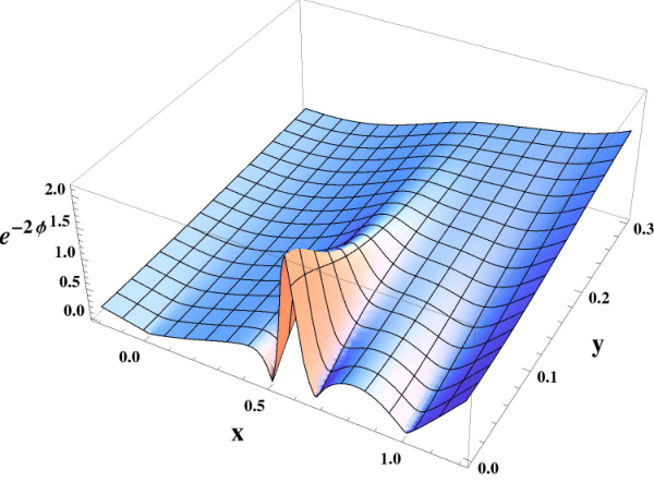
Plots illustrating the solution are shown in Figure 4. The qualitative features are the same as for the 3-pole solution: The metric factors are positive and the fields satisfy the desired regularity conditions throughout, except for the poles where they behave as derived in sec. 3.9.
4.3 Relation to 5-brane webs
We have argued already briefly in [4] that our supergravity solutions can be identified with fully localized intersections of 5-branes, and the detailed derivations presented in this paper provide the justification for the arguments used in [4]: By construction, our supergravity solutions have the correct superconformal symmetry, and by the results of sec. 3.8 the parameter count precisely matches the parameter count of five-brane webs in the conformal limit. Moreover, as the discussion of sec. 3.10 shows the solutions also have the correct external states and the parameters can be directly translated to those specifying a 5-brane intersection.
Many other features of the solutions admit a natural interpretation in the context of 5-brane intersections as well. The minimal number of poles being three, as discussed in sec. 3.3, corresponds to the fact that three external branes are needed to produce a codimension-1 intersection. Moreover, there are no solutions with either only D5 charge or only NS5 charge. From (3.14) we have . Therefore, if the are either all real or all imaginary, vanishes for all , which implies that everywhere and the solution degenerates. Regular solutions therefore necessarily involve D5 and NS5 charge, and this corresponds to the fact that D5 and NS5 charges are needed to realize a codimension-1 intersection with 5-branes.
The identification of our solutions with 5-brane intersections certainly suggests a holographic relation to the 5d SCFTs obtained by taking the conformal limit of 5-brane webs describing 5d supersymmetric gauge theories [9, 10]. Holographic relations usually involve some form of a large- limit, and we indeed note that the charges of the external 5-branes in our solutions are assumed to be large for the supergravity description to be valid. There is therefore no constraint from charge quantization, similarly to the familiar case of e.g. SYM and its dual. Generically, the brane intersections described by our solutions therefore involve both, large D5 charge and large NS5 charge. Brane webs related by the duality of type IIB string theory describe the same field theory, and in type IIB supergravity this is enhanced to an symmetry.55 5 Not to be confused with the automorphisms of the upper half plane (c.f. sec. 3.7). Solutions related by automorphisms of the upper half plane are actually equivalent solutions, while solutions related by duality transformations are generally not. We thus expect solutions related by to describe field theories with the same “large-” limit.
We will now use the explicit solutions with three and four poles for a more explicit discussion and to illustrate further points. The solutions with three poles correspond to 5-brane intersections with three external 5-branes, with charges given by (3.43). They have a total number of four parameters, corresponding to the choice of charges subject to charge conservation. For the field theory interpretation, further reduces the number of parameters by , which leaves only one free parameter. Indeed, a generic 3-fold intersection of 5-branes can be mapped to the form shown in Figure 5 by an transformation. This “-junction” is obtained by combining copies of the basic 5-brane junction with external charges , and (in all in-going convention) and allows for a large- limit. A choice of parameters for the supergravity solution to realize this form of the web via (4.1), (4.2) is
| (4.12) |
Brane webs of the form shown in Figure 5 have been identified in [22] as five-dimensional uplifts of the four-dimensional theories, obtained by wrapping M5-branes on a sphere with 3 punctures. For the field theory interpretation it is crucial whether and how the external 5-branes defining the intersection end on 7-branes. In [9, 10] the external 5-branes were taken to be semi-infinite, but one can also terminate them on 7-branes such that they are of finite extent in the plane in which the brane web is drawn [11]. Taking groups of 5-branes to end on the same 7-brane yields a different field theory than having each 5-brane semi-infinite or terminate on its own 7-brane, and for the intersection of Figure 5 various options were discussed in [22].
In our solutions we only see the external 5-brane geometries with no indication for the presence of 7-branes, and at least at the level of disk solutions there are also no obvious moduli corresponding to the choice which 5-branes terminate on which 7-brane. This suggests that the solutions correspond to the original form of the brane webs and intersections, where the external 5-branes are indeed semi-infinite [9, 10]. However, one could also argue that our solutions only cover the near-intersection limit, where the external 7-branes may not be directly accessible and more indirect methods will be required to precisely pin down the dual field theory. We will leave a more detailed investigation for the future and leave this question open for the remaining discussion.
The lift of the isolated 4d theories to 5d via intersections of the form in Figure 5 offers a chance to find deformations that permit a Lagrangian description as gauge theories in the IR, and such deformations have been constructed in [23]. For the case where each external 5-brane ends on a separate 7-brane, it results in a web describing the quiver
| (4.13) |
That is, a gauge theory with product gauge group , with one hypermultiplet in the bi-fundamental representation for each pair of adjacent gauge group factors and in addition massless hypermultiplets in the fundamental representation of along with massless hypermultiplets in the fundamental of . The 5-brane intersection only has one large parameter controlling both D5 and NS5 charge, and we see that in this case it also translates to two large parameters in the field theory defining the UV fixed point: the length of the quiver and the rank of the largest gauge group factor.
Moving on to 4 external branes, the 5-brane intersection with the external charges of sec. 4.2 is shown on the left hand side in Figure 6. Once again the field theory interpretation depends on whether and how the external 5-branes end on 7-branes. Taking and all 5-branes within each external 5-brane stack to end on the same 7-brane would yield a 5-brane construction for the USp() theory [8], while the original form of the webs with no 7-branes again leads to long quivers: The configuration is SL(2,) dual (up to a rescaling of the charges and ) to the intersection shown on the right hand side in Figure 6. Without the introduction of 7-branes this intersection has been discussed already in [10], and a deformation of the fixed-point SCFT to a gauge theory is described by the quiver
| (4.14) |
This example explicitly exhibits the presence of two independently large parameters, the rank of the gauge group and the length of the quiver, corresponding to the D5 charge and NS5 charge in the brane intersection. Moreover, we note that the number of matter fields is directly linked to the rank of the gauge group factors, and the large- limit is a form of a Veneziano limit rather than a ‘t Hooft limit.
5 The annulus
In this section, we shall investigate the existence of supergravity solutions when has the topology of an annulus, or equivalently of a finite cylinder. This is the next-simplest topology after the case of the disk, since the annulus has genus zero but two boundary components. We shall provide an explicit parametrization of the differentials under the assumption that these differentials are single-valued in and no axion monodromy is allowed. We will explicitly construct the functions as well and derive the general physical regularity conditions.
We have used a combination of analytical and numerical methods to explore whether the physical regularity conditions on the supergravity fields can all be satisfied simultaneously for the annulus. These explorations are not exhaustive, but the outcome so far has consistently been negative, and no example of a physically regular solution has been found to date. We have no analytical proof that such solutions cannot exist, but the regularity conditions are structurally different when there are multiple boundary components and the negative results so far may well be due to the fact that such solutions do generally not exist. We will leave a more systematic analysis for the future and turn to Riemann surfaces with non-trivial topology and a single boundary component in the next section.
5.1 Parametrization of the annulus
Compared to the situation of the disk, the annulus has two new features. First, the annulus has two disconnected boundary components instead of one for the disk; second the annulus has a non-trivial fundamental group .
The function theory on the annulus, which we need to construct the differentials and the associated functions , is conveniently obtained in terms of the function theory on the double surface. The annulus may be represented in the complex plane by a rectangle with two opposing edges periodically identified. The double surface of the annulus is a torus whose periods may be chosen to be 1 and and whose modulus is purely imaginary with . The surface and its boundary may then be represented by,
| (5.1) |
both periodically identified under , as represented in Figure 7. We choose by symmetry across the real axis, such that and . Complex conjugation is the anti-conformal involution which maps between the components of in the upper and lower half planes. We may view as the quotient , and the boundary as the fixed set under .
5.2 The function
To investigate the existence of physically regular supergravity solutions, we closely follow the general strategy outlined in subsection 2.4, and begin with the construction of the holomorphic function . To construct we use the scalar Green function on which vanishes whenever is on . To construct , we make use of the scalar Green function on the double surface ,
| (5.2) |
where is the Jacobi -function. By construction, is a real and doubly periodic function,
| (5.3) |
in view of the standard translation properties of the Jacobi -function,
| (5.4) |
The corresponding Green function on the annulus is given by,
| (5.5) | |||||
The properties of reality and double periodicity of (5.3) ensure whenever , so that vanishes on both boundary components of .
The function for the annulus with modulus may be inferred from the electrostatic potential obtained by adding the contributions from an array of positive unit charges placed at points with , and satisfying . Therefore, the general electrostatic potential used in (2.18) takes the from,
| (5.6) |
To extract the holomorphic function , we use the fact that is real and harmonic in away from to split (5.6) into a sum of holomorphic and anti-holomorphic parts in ,
| (5.7) |
leaving a constant phase factor undetermined. This expression is automatically single-valued under , and is single-valued under provided we impose the following condition on the points ,
| (5.8) |
We recognize this relation as the divisor condition for meromorphic functions on the torus, applied to the special case where the zeros and poles come in complex conjugate pairs. The condition implies that we must have , since it is clearly unattainable with in view of the requirements that at least one of the zeros should lie in the interior of .
5.3 The differentials
To construct the meromorphic differentials , we begin by splitting into two complex conjugate functions ,
| (5.9) |
The splitting is not unique, as a common factor of a real function to cancels out in . The irreducible solution is given as follows,
| (5.10) |
Neither function is single-valued on . The differentials are given in terms of a meromorphic function on by (2.21) so that,
| (5.11) |
Applying the general conditions on the meromorphic 1-forms of subsection 2.4.2 to the case of the annulus allows us to narrow the choices of as follows.
Since cannot vanish in the interior of in view of the condition , the function cannot have zeros in the interior of . Furthermore, cannot have poles in the interior of since otherwise the functions would have monodromy in the interior of . Therefore, all zeros and poles of must be on the boundary . Zeros on the boundary may be viewed as corresponding to a degenerate situation of the general case where all zeros are in the interior, and we shall therefore assume that no zeros occur on the boundary, so that has no zeros at all. Since meromorphic differentials on the torus have equal numbers of zeros and poles, must have precisely poles on . As a result, the zeros of in the interior of are precisely the zeros of .
Finally, we shall adopt the condition (2.22) which for the torus reads,
| (5.12) |
With the above assumptions, we parametrize by its poles at points with distributed amongst the two boundary components of given in (5.1). Combining the above conditions, we find the following expressions for the differentials ,
| (5.13) |
where is a complex constant while are given by,
| (5.14) |
By construction, and with the help of (5.4), the differentials are invariant under , but their invariance under requires the extra conditions,
| (5.15) |
These conditions on combined imply the divisor relation (5.8) derived earlier.
It remains to enforce the conjugation condition of (5.12). In the special case where all the poles lie on the real boundary component, the condition amounts to requiring . In the general case when poles are allowed to lie on both boundary components, enforcing (5.12) is more delicate, and we have instead the general relation,
| (5.16) |
where is constant and is subject to the relation . Satisfying the combination of the conditions (5.15) and (5.16) thus provides single-valued meromorphic differentials on the annulus which satisfy the conjugation condition (5.12).
5.4 The functions
In this subsection, we shall integrate the differentials to obtain the functions . The product representation (5.13) obtained in the preceding subsection is inconvenient to carry out this integration. Instead, we shall derive here an equivalent representation as a sum over meromorphic Abelian differentials which may be easily integrated.
Since the meromorphic differentials of (5.13) are single-valued on the double surface , the sum of their residues at the poles must vanish, and the differentials can be expressed as a sum over meromorphic Abelian differentials , which are single-valued under , and transform under by a constant shift,
| (5.17) |
The residues may be obtained from (5.13) by matching poles and are given by,
| (5.18) |
The presence of the constants is due to the fact that the torus has a one-dimensional space of holomorphic Abelian differentials which, in local complex coordinates , is generated by the differential . A meromorphic one-form such as will generically have a non-trivial component along . The values of may be obtained by using (5.12) and the vanishing of at any of the zeros ,
| (5.19) |
The integrals of are now easily computed, and we have,
| (5.20) |
where are complex integration constants.
To secure useful conjugation properties, care is needed in the choice of branch cuts for the logarithm. Given a choice of branch cut in , the proper branch cut in is actually more properly written as,
| (5.21) |
where the branch cuts chosen in are now the same. With this choice, we may use a constant gauge transformation of the flux field to set to zero, just as we did in the case of the upper half plane, upon which we obtain the following conjugation relation,
| (5.22) |
In the next subsection, we obtain the conditions under which on the boundary.
5.5 Conditions for on the boundary
The general arguments of subsection 2.4.2 along with the conjugation conditions (5.12) and (5.22) lead us to conclude that is constant along any line segment free of poles on the boundary . To enforce the boundary condition on the entire boundary, it will therefore suffice to enforce on any one line segment free of poles on each boundary, and then require that the monodromy across every pole on that boundary component vanishes.
We begin by requiring the vanishing of the monodromy of across an arbitrary pole along the contour illustrated in Figure 8. To keep track of the behavior of the functions near their branch cuts, we introduce defined by,
| (5.23) |
where for poles on the real line and for poles on the second boundary component. The resulting has a small positive real part and an imaginary part reflecting the contours in Figure 8. To find the jump conditions we start out from,
| (5.24) | |||||
where
| (5.25) |
with the half circle part of the contour around the pole . For the change in we find
| (5.26) |
which leads to
| (5.27) | |||||
Working this out more explicitly yields
| (5.28) | |||||
Using and the quasi-periodicity of the functions, the log terms in the round brackets can be evaluated more explicitly. The integrals in for the jump are restricted to a half circle around the pole, which means the integrand can be expanded for . Upon explicit evaluation we find that the contribution from precisely matches the change in and merely produces an overall factor of . Altogether, we find
| (5.29) | |||||
The sum then evaluates to
| (5.30) | |||||
The sum manifestly vanishes if and all poles are on one boundary component. In this case, the conditions (5.29) simplify considerably, and we have,
| (5.31) |
which is analogous to the condition for the disk in (3.25).
5.6 Minimal number of poles
For the case of the disk, a minimum of three poles in was required in order to have a single zero in the upper half plane, lest the solution be trivial. For the case of the annulus, the number of zeros of must equal the number of its poles instead. We shall now analyze the minimal number of zeros and poles required for the annulus case.
When all the poles of are on one boundary component the requirement implies , and hence both conditions in eq. (5.15). Periodicity of the functions as requires . This is one complex condition due to , and is equivalent to the condition,
| (5.32) |
where is any one of the zeros of (cf. (5.19)).
The condition has no solutions with two poles on the same boundary, since this would require two zeros in the interior of , whose imaginary parts add up to a non-zero multiple of by conditions (5.15). The only possibility would be to have their imaginary parts both equal to , but this implies in turn that both zeros are on the boundary of leading to an unphysical solution.
The condition can be solved with two poles and two zeros inside the annulus, provided we have one pole on each boundary component. Without loss of generality, we use translation invariance to set and . Assuming furthermore that , the condition (5.30) with then implies and thus . The condition , via (5.32) and with , then implies,
| (5.33) |
This equation only has two unacceptable solutions below the real line, and no solutions for inside the annulus. We thus find that there are no solutions with two poles, and that at least three poles are a necessary condition for a physically regular solution to exist.
5.7 Investigating solutions with at least three poles
Starting with 3 poles it becomes considerably more involved to disentangle the collection of conditions developed earlier. While we cannot offer an exhaustive analysis here, we shall present the conclusions we draw from a partial numerical analysis we have carried out.
With poles for , the divisor conditions (5.15) allow for all poles to be distributed over both boundary components including the case where all poles are on one boundary component. Our numerical analysis of the conditions , which are required to make single-valued under , in the case of poles appears to exclude systematically the cases where all poles of are not on the same boundary. Indeed, when poles occur on both boundary components, we find that the condition , for a given distribution of poles on the boundary and for zeros inside , always forces one of the remaining zeros of to be outside of . So far, we have no analytical proof of this claim.
With poles, and all poles on a single boundary component, it is possible to satisfy the conditions and have all zeros of in the interior of . A simple family of such solutions may be obtained by choosing the distribution of poles and zeros to be invariant under translations, and given by,
| (5.34) |
For given the zeros are well in the interior of . Therefore, by continuity, we know that there will exist an open set in the space of all solutions which contains the above solution as a point, and has maximal dimension, given by the real coordinates of poles , the complex coordinates of zeros, minus the complex condition , and minus the real divisor condition, adding up to .
Having established that there are at least the partial solutions exhibited above, we more generally explored configurations with all poles on a single boundary, and showed numerically that the conditions for continuity of the function across the poles, namely the conditions for , may be solved as well. The solutions to all these conditions combined now provide configurations for which all zeros of are in the interior of , the condition is satisfied, and is constant on each boundary component.
There now remain two further conditions to be implemented, namely that on both boundary components. There is a natural free parameter, namely the integration constant of the composite holomorphic function which may be used to set on one boundary component. The value of on the other boundary component is then determined by the parameters of the solution. Our numerical analysis for the case of poles appears to show that the condition can not be satisfied simultaneously on both boundary components. Rather, the difference between the values of on the boundary with no poles and on the boundary with all poles appears to consistently be positive. Again, at this time, we have no analytical proof of this claim, but hope to return to this question in the future.
If the indications from the numerical analyses carried out so far are correct, then the annulus may not support physically regular solutions in the absence of axion monodromy. More generally, we may speculate that the obstruction to the existence of solutions resides in the presence of more than one boundary component, in the case of the annulus as well as for surfaces of arbitrary genus.
6 Riemann surfaces of arbitrary topology
In this last section, we shall construct suitable differentials for general Riemann surfaces, and spell out the conditions required for the corresponding supergravity solutions to be physically regular. The final equations are so complicated, however, that so far we have not succeeded in constructing acceptable solutions, even numerically.
Consider an orientable Riemann surface of genus with boundary components which topologically are circles. Functions and differential forms on may be constructed in terms of functions and differential forms on the double surface , equipped with an anti-conformal involution which we shall denote by (for a standard reference, see [24]). The boundary of is fixed, point by point, under so that . We may view as the quotient . The genus of is related to the genus and the number of boundary components of the original surface by the standard relation,
| (6.1) |
This construction is depicted in Figure 9 for the case and . The conventions for the basis of homology cycles indicated in the figure will be given in section 6.2 below.
6.1 Generalizing the electrostatics analogy
The electrostatics analogy, used to construct the function for the cases of the upper half plane and the annulus, may be generalized without complications to the case of an oriented Riemann surface of arbitrary genus , and an arbitrary number of boundary components the topology of each of which is that of a circle. In the electrostatics analogy, we seek first to construct an electrostatic potential which vanishes on the boundary and is strictly positive everywhere in the interior of . To achieve such an electrostatic potential, we ground the system to zero potential on every component of and place an arbitrary arrangement of positive charges in the interior of . By the min-max principle for harmonic functions, used already earlier in subsection 2.4, the potential is then guaranteed to be positive everywhere in the interior of .
Mathematically, we start from the original Riemann surface of genus with boundary components and construct its double endowed with a conformal involution . To obtain a potential which is strictly positive in the interior of , and which vanishes on the boundary , we place an arrangement of an arbitrary number of positive electric charges at arbitrary points in the interior of , with , and place mirror charges at the mirror locations . Since by construction the potential is odd under the involution , it is guaranteed to vanish on the boundary . Since all charges on are positive, and the potential vanishes on , we use again the min-max principle for harmonic functions to argue that must then be strictly positive in the interior of , just as we had already done in the case of the upper half plane and the annulus. Clearly, such solutions will always exist. To obtain explicit formulas for , we shall provide the necessary mathematical set-up in the next subsection.
6.2 Double surface and involution
We shall sort the homology cycles on the double surface , and their dual holomorphic 1-forms, according to their parity under . Our labeling of the cycles generalizes to arbitrary and the labeling indicated in Figure 9 for and , and we have [24],
| cycles belonging to | (6.2) | ||||
| cycles conjugate under | |||||
| boundary cycles for | |||||
| conjugate cycles for |
There is one further boundary component, which is homologically trivial on . Throughout, the indices , , will run over the ranges given in (6.2) and we shall conveniently use the composite index . We define the involution matrix by,
| (6.3) |
where and are the identity matrices respectively in dimensions and . The cycles may be arranged to have definite parity under , which we choose as follows,
| (6.4) |
The normalization of the holomorphic 1-forms on the -cycles and their corresponding behavior under the pull-back of the involution to 1-forms, are given as follows,
| (6.5) |
where is the complex conjugate of . The period matrix of is defined by,
| (6.6) |
By the Riemann bilinear relations, is symmetric in and has positive definite imaginary part. As a result of the action of on the cycles in (6.4), and on the holomorphic 1-forms in (6.5), satisfies further relations. To derive them, we make use of the formulas,
| (6.7) |
Combining these results, we proceed by the following manipulations,
| (6.8) |
The result is the conjugation condition on ,
| (6.9) |
Decomposing into real matrices decomposes (6.9) into and . The conjugation condition guarantees that the genus Riemann surface with period matrix indeed has an involution . It is equivalent to a reality condition on up to conjugation by , and reduces the number of free parameters of to half.
6.3 The function
To construct we follow the strategy of section 2.4. We construct a general electrostatic potential which is odd under the involution and which is strictly positive in the interior of . To do so we place an arbitrary arrangement of positive charges in , and add their image charges in . The scalar Green function on may be chosen as follows,
| (6.10) |
where is the prime form on . The prime form is a holomorphic form of weight in and , which satisfies , and whose asymptotics is given by for near . For its definition in terms of -functions, and further properties, see for example [24, 25]. Monodromy transformations act as follows,
| (6.11) |
Under the involution , the prime form behaves as follows,
| (6.12) |
While the scalar Green function is not uniquely defined, since it would correspond to the electrostatic potential of a single electric charge, the Green function for a pair of opposite unit charges placed at conjugate points and is well-defined, and given by,
| (6.13) |
Its expression in terms of the prime form and Abelian integrals simplifies as follows,
| (6.14) |
In order to produce a function without branch cuts the positive charges should be chosen to be all equal to unity, giving the following general solution for the electrostatic potential,
| (6.15) |
To split the holomorphic dependence in from the anti-holomorphic dependence we begin by splitting the line integral using (6.7),
| (6.16) |
Splitting off the holomorphic dependence in now clearly amounts to splitting off the dependence in from the dependence in . Using furthermore the fact that and that commutes with , and exponentiating the holomorphic part to obtain , we find,
| (6.17) |
While was single-valued on , the splitting into and its complex conjugate generally introduces monodromy by phase factors. To obtain a single-valued will necessitate divisor relations on the zeros , which we now obtain.
The monodromy properties of the function as is moved around the homology cycles and on are readily evaluated using (6.11). We state here, without detailed derivation, the conditions for the absence of monodromies around all homology cycles,
| (6.18) |
where the column matrices have integer entries, restricted in the following way,
| (6.19) |
where the integers for and for are arbitrary. These conditions state that the zeros and poles indeed satisfy the customary divisor condition of a meromorphic function on a Riemann surface which possesses an involution (see for example [24, 25]).
6.4 The differentials
To construct the differentials we split the meromorphic function on into the ratio of two conjugate multiple-valued holomorphic differentials on as follows,
| (6.20) |
The differential form has its zeros at , while has its zeros at . The splitting of the prime form factors in (6.17) is manifest. To split the exponential factor, we make use of (6.16) but with replacing . The splitting of is now manifest, and we find,
| (6.21) | |||||
where the point lies on the boundary of , so that we have . As constructed above, the differential forms have weight in .
Next, we construct the holomorphic differentials to be well-defined and single-valued on . The basic equations for are as follows,
| (6.22) |
The differential form must have weight and has neither zeros nor poles in the interior of , so that its poles and zeros are on . As in the cases of the upper half plane and the annulus, we shall view any real zeros as degenerations of pairs of conjugate zeros to the boundary. We shall denote the poles by with . To have well-defined and single-valued meromorphic differentials on , the number of their poles and zeros are related as follows,
| (6.23) |
For , one may view the positions of the poles and of of the zeros as arbitrary, while the remaining zeros are determined by the divisor condition for forms of weight . Taking these considerations into account, we obtain the following expressions for ,
| (6.24) | |||||
where are given by,
| (6.25) |
The holomorphic form has weight and has neither zeros nor poles. Its role in (6.24) is to guarantee that the forms have the weight in , and are single-valued. The monodromy of the form around -cycles on is trivial; its monodromy around -cycles and its expression in terms of the prime form are given below,
| (6.26) |
Here, is the Riemann vector on the surface . Choosing the base point to be invariant under the involution , the Riemann vector is real in the Jacobian . The conjugation property of under conjugation follows that of the prime form and we have,
| (6.27) |
Using it, we readily establish the conjugation relations for the differentials,
| (6.28) |
The transformation laws given above for the prime form, the exponential in (6.24), and allow us to compute the monodromies of around and cycles. Requiring the monodromies to vanish around all cycles imposes the following conditions on ,
| (6.29) |
where and are column matrices whose entries are integers which satisfy,
| (6.30) |
where the integers for and for are arbitrary. These conditions imply the relations for single-valuedness of of (6.18) with,
| (6.31) |
The total number in (6.29) is real conditions.
6.5 The functions
To integrate we decompose these differentials onto the following Abelian differentials of the third kind,
| (6.32) |
with simple poles at and with unit residues of opposite signs. In view of the cancellation of the sum of the residues at the poles , all dependence on cancels out, and we have the following decomposition,
| (6.33) |
where are the coefficients of the holomorphic one-forms on . The residues satisfy,
| (6.34) |
and their values may be read off from the product representations in (6.24),
| (6.35) |
The coefficients may be obtained by evaluating (6.33) at of the zeros, denoted by , of and of the zeros of ,
| (6.36) |
and then solving each linear system in turn. The functions are obtained by integrating (6.33),
| (6.37) |
The functions do not necessarily have to be single-valued on . Indeed, monodromy of by constant shifts, as given in (2.10) subject to the condition (2.11), is allowed as it gives rise to single-valued supergravity fields. We shall now investigate the conditions this kind of allowed monodromy imposes on the parameters of the holomorphic functions . First, by comparing the complex conjugate of the second line in (6.36) with the first line of (6.36), we obtain the relation,
| (6.38) |
or simply in matrix notation. When the index corresponds to a boundary cycle, this relation generalizes the one obtained for the annulus in (5.19). Second, the monodromies around cycles and are given by,
| (6.39) |
There are no conditions on the monodromy around cycles, as such cycles extend beyond the surface . Thus, the conditions for allowed monodromy around these cycles are given by,
| (6.40) |
or simply and in matrix notation. Combining these relations, we obtain the following constraints on the parameters of the solution, expressed here in matrix notation,
| (6.41) |
Translated in components, the first set of equations become,
| (6.42) |
while the second set of equations gives in terms of the residues and the poles . We see that, by contrast with the case of the annulus, for higher genus the parameters need not be forced to vanish by the monodromy conditions alone.
6.6 The conditions required for on the boundary
The general arguments of subsection 2.4.2 guarantee that is piecewise constant on any line segment of the boundary which is free of poles. The condition for continuity of the function across a pole is given by the same arguments as in the case of the upper half plane and the annulus. Here, we shall specialize to the case where we have a single boundary component and hence , since the expressions considerably simplify in this case. We shall also assume that the condition for single-valuedness around cycles has been imposed, so that . The conditions are local around , and are given as follows,
| (6.43) |
When only a single boundary component is present, the vanishing of on may be achieved by solving for the integration constant of the holomorphic function . When has boundary components, there are further real conditions required to guarantee the vanishing of on each boundary component.
This completes the construction of the ansatz for general Riemann surfaces and the derivation of the regularity conditions. We leave a detailed investigation of the existence of solutions with non-trivial topology for the future and close by noting that, based on the numerical investigations for the annulus described in subsection 5.7, we may speculate that no solutions will exist if has multiple boundary components.
7 Discussion
In this paper we have constructed a large family of Type IIB supergravity solutions which are candidates for holographic duals to five-dimensional superconformal field theories. The space-time of these solutions consists of the manifold warped over a two-dimensional Riemann surface with boundary. The supergravity solutions preserve sixteen supersymmetries and give a holographic realization of the superconformal algebra. Unlike corresponding solutions in dimensions 3, 4 and 6, there is no asymptotic enhancement of the supersymmetry, in accord with the fact that there exist no five-dimensional superconformal theories with thirty two supersymmetries.
The solutions become singular at isolated points on the boundary of the Riemann surface, where the poles in the differentials which characterize the solutions are located. The singularities have a clear physical interpretation, as the supergravity fields near the poles take the form of the singular “near horizon” limit for a five-brane. This gives a natural identification of the poles as remnants of the external five-branes which are used to construct brane web realizations of five-dimensional field theories. The symmetry of our solutions implies that we are describing the conformal fixed points where the web collapses to a five-brane intersection with all branes intersecting at a single point. This offers a clear path to identifying the dual SCFTs, as we have discussed for example solutions with three and four poles corresponding to intersections with three or four external branes.
For the large class of explicit solutions presented in this work we have assumed the topology of the Riemann surface to be that of a disk. For higher topologies, we have presented the general set-up for the construction of physically regular supergravity solutions, but we have not shown that such solutions exist. For the case of the annulus, our numerical investigations point in the direction that physically regular solutions without axial monodromy may not exist, though we have no analytical proof. From the analysis and numerical results for the annulus, it is natural to speculate that physically regular solutions will exist only when there is precisely one boundary component. Whether solutions with higher genus exist, and what their physical interpretation in terms of five-brane webs may be, is at this time an open question, to which we hope to return in the future.
Many aspects of the supergravity solutions that we have constructed and the proposed dual superconformal field theories to these solutions remain to be explored as well. We end the paper with a discussion of some of the open questions and avenues for future research.
One might wonder whether the presence of the singularities at the poles of the differentials , and the fact that the supergravity solution near the singularities approaches the near horizon limit of a five-brane, can invalidate the interpretation of the solution as a dual of a five-dimensional theory. It is a natural next step to study field theory observables holographically in order to address this question.
In the AdS/CFT correspondence the spectrum of operators and correlation functions are the most direct observables which can be obtained by considering the KK-spectrum of linearized perturbations and Witten diagrams, respectively. However, due to the fact that the space is warped over the Riemann surface this analysis is considerably more complicated than in more familiar cases such as the solution of Type IIB. It would be interesting to investigate the operator spectrum for our warped solutions, as little is known about the operator spectrum of the five dimensional SCFTs.
Other CFT observables such as the entanglement entropy can be calculated more straightforwardly using the Ryu-Takyanagi prescription [26, 27]. Such a calculation for a spherical region has been performed for the singular Type IIA supergravity solutions in [28], and we are currently investigating the holographic entanglement entropy for the solutions presented in this paper [29]. Preliminary results suggest that the presence of the poles does not obstruct the holographic computations of either the entanglement entropies or of the free energy directly.
Another interesting prospect for the future is to further generalize our solutions. S-duality acts naturally on the holomorphic functions which parameterize them, but the solutions presented in this paper all exhibit vanishing monodromy under the S-duality group. This means that as one moves along a closed loop on the Riemann surface all supergravity fields come back to the same value. It is well known, however, that seven-branes induce nontrivial monodromies on some supergravity fields. For example, a D7-brane induces a shift of the axion along a closed contour enclosing the D7-brane in the two transverse directions. We note that seven-branes can naturally be incorporated into five-brane webs [11] and they are indeed needed for the most general construction of five dimensional field theories and their moduli spaces. Consequently, it is an interesting question whether it is possible to incorporate seven-branes and their monodromies into the framework of our solutions. We plan to address this question in future work.
Acknowledgements
We are happy to thank Andreas Karch for collaboration on an earlier paper that led to the present work, and to Oren Bergman and Diego Rodriguez-Gomez for extensive and helpful discussions on five-brane webs. We also acknowledge the Aspen Center for Physics, which is supported by National Science Foundation grant PHY-1066293, for hospitality during the workshop “Superconformal Field Theories in ” and thank the organizers and participants for the enjoyable and inspiring conference. The work of all three authors is supported in part by the National Science Foundation under grant PHY-16-19926.
Appendix A Absence of poles for in the interior of
In the main part of the paper we have assumed that all poles of are located on the boundary of . In this appendix we shall rule out the presence of poles in in the interior of . The arguments are local. For concreteness, we shall present them here for the explicit solutions on the upper half plane, but their locality guarantees that their validity extends to surfaces of arbitrary topology.
The starting point for the construction of the physically regular supergravity solutions is the function which, for the upper half plane, is given by,
| (A.1) |
To construct the differentials from , we had originally assumed that all zeros of become zeros of , while all poles of become zeros of . But this is not the most general possibility available for given . Indeed, some of the zeros of can actually become poles of and the accompanying complex conjugate poles of can become poles of . We illustrate this by singling out the pair of zeros and poles of , ,
| (A.2) |
The locality of the argument will guarantee that it applies equally well when more than one pair of zeros and poles are reversed. We now construct accordingly,
| (A.3) |
Note that we have poles to ensure regularity at infinity. We automatically have in the interior of , since this condition was already guaranteed by the form of alone. Recall that the pre-factor of is present (previously denoted ) to enforce the conjugation property , which is essential for the piece-wise vanishing of along the real line. Decomposing into partial fractions, we have,
| (A.4) |
and integrating,
| (A.5) |
Next, is computed by first evaluating its derivative,
| (A.6) |
The dominant behavior near the pole in the upper half plane is carried by which diverges logarithmically there, while is regular. Hence near we have,
| (A.7) |
This implies that the leading behavior of is given by
| (A.8) |
Hence, near , the function is negative and divergent. Hence fails to be positive everywhere in the interior of and the solution fails to be regular.
References
- [1] E. D’Hoker, M. Gutperle, A. Karch and C. F. Uhlemann, Warped in Type IIB supergravity I: Local solutions, JHEP 08 (2016) 046, [1606.01254].
- [2] V. G. Kac, Lie Superalgebras, Adv. Math. 26 (1977) 8–96.
- [3] S. Shnider, THE SUPERCONFORMAL ALGEBRA IN HIGHER DIMENSIONS, Lett. Math. Phys. 16 (1988) 377–383.
- [4] E. D’Hoker, M. Gutperle and C. F. Uhlemann, Holographic duals for five-dimensional superconformal quantum field theories, Phys. Rev. Lett. 118 (2017) 101601, [1611.09411].
- [5] N. Seiberg, Five-dimensional SUSY field theories, nontrivial fixed points and string dynamics, Phys. Lett. B388 (1996) 753–760, [hep-th/9608111].
- [6] K. A. Intriligator, D. R. Morrison and N. Seiberg, Five-dimensional supersymmetric gauge theories and degenerations of Calabi-Yau spaces, Nucl. Phys. B497 (1997) 56–100, [hep-th/9702198].
- [7] A. Brandhuber and Y. Oz, The D-4 - D-8 brane system and five-dimensional fixed points, Phys. Lett. B460 (1999) 307–312, [hep-th/9905148].
- [8] O. Bergman and D. Rodriguez-Gomez, 5d quivers and their AdS(6) duals, JHEP 07 (2012) 171, [1206.3503].
- [9] O. Aharony and A. Hanany, Branes, superpotentials and superconformal fixed points, Nucl. Phys. B504 (1997) 239–271, [hep-th/9704170].
- [10] O. Aharony, A. Hanany and B. Kol, Webs of (p,q) five-branes, five-dimensional field theories and grid diagrams, JHEP 01 (1998) 002, [hep-th/9710116].
- [11] O. DeWolfe, A. Hanany, A. Iqbal and E. Katz, Five-branes, seven-branes and five-dimensional E(n) field theories, JHEP 03 (1999) 006, [hep-th/9902179].
- [12] A. Hanany and E. Witten, Type IIB superstrings, BPS monopoles, and three-dimensional gauge dynamics, Nucl. Phys. B492 (1997) 152–190, [hep-th/9611230].
- [13] F. Apruzzi, M. Fazzi, A. Passias, D. Rosa and A. Tomasiello, AdS6 solutions of type II supergravity, JHEP 11 (2014) 099, [1406.0852].
- [14] H. Kim, N. Kim and M. Suh, Supersymmetric AdS6 Solutions of Type IIB Supergravity, Eur. Phys. J. C75 (2015) 484, [1506.05480].
- [15] H. Kim and N. Kim, Comments on the symmetry of AdS6 solutions in string/M-theory and Killing spinor equations, Phys. Lett. B760 (2016) 780–787, [1604.07987].
- [16] E. D’Hoker, J. Estes and M. Gutperle, Exact half-BPS Type IIB interface solutions. I. Local solution and supersymmetric Janus, JHEP 06 (2007) 021, [0705.0022].
- [17] E. D’Hoker, J. Estes and M. Gutperle, Gravity duals of half-BPS Wilson loops, JHEP 06 (2007) 063, [0705.1004].
- [18] E. D’Hoker, J. Estes, M. Gutperle and D. Krym, Exact Half-BPS Flux Solutions in M-theory. I: Local Solutions, JHEP 08 (2008) 028, [0806.0605].
- [19] E. D’Hoker, Exact M-Theory Solutions, Integrable Systems, and Superalgebras, SIGMA 11 (2015) 029, [1411.6170].
- [20] J. B. Gutowski and G. Papadopoulos, On supersymmetric AdS6 solutions in 10 and 11 dimensions, 1702.06048.
- [21] J. X. Lu and S. Roy, An SL(2,Z) multiplet of type IIB super five-branes, Phys. Lett. B428 (1998) 289–296, [hep-th/9802080].
- [22] F. Benini, S. Benvenuti and Y. Tachikawa, Webs of five-branes and N=2 superconformal field theories, JHEP 09 (2009) 052, [0906.0359].
- [23] O. Bergman and G. Zafrir, Lifting 4d dualities to 5d, JHEP 04 (2015) 141, [1410.2806].
- [24] J. Fay, Theta functions on Riemann surfaces, Springer Lecture Notes in Mathematics 352 (1973) 781–846.
- [25] E. D’Hoker and D. H. Phong, The Geometry of String Perturbation Theory, Rev. Mod. Phys. 60 (1988) 917.
- [26] S. Ryu and T. Takayanagi, Holographic derivation of entanglement entropy from AdS/CFT, Phys. Rev. Lett. 96 (2006) 181602, [hep-th/0603001].
- [27] S. Ryu and T. Takayanagi, Aspects of Holographic Entanglement Entropy, JHEP 08 (2006) 045, [hep-th/0605073].
- [28] D. L. Jafferis and S. S. Pufu, Exact results for five-dimensional superconformal field theories with gravity duals, JHEP 05 (2014) 032, [1207.4359].
- [29] M. Gutperle, C. Marasinou, A. Trivella and C. F. Uhlemann, to appear, .