跳到论文正文
W Papers独立论文阅读器 arXiv:1703.08115 论文正文 计算阅读时间 · 0%
引用这篇论文根据当前论文元数据生成,正式投稿前建议核对。


License: arXiv.org perpetual non-exclusive license
arXiv:1703.08115v1 [eess.SY] 23 Mar 2017

Relaxed Bi-quadratic Optimization for Joint Filter-Signal Design in Signal-Dependent STAPThanks: S. M. O’Rourke is with the Sensors Directorate, US AFRL, WPAFB, OH and the University of California, Irvine. Email: sean.orourke.3@us.af.milThanks: M. Rangaswamy is with the Sensors Directorate, US AFRL, WPAFB, OH. Email: muralidhar.rangaswamy@us.af.milThanks: P. Setlur is affiliated with the Wright State Research Inst. as a research contractor for the US AFRL, WPAFB, OH. Email: pawan.setlur@wright.eduThanks: A. L. Swindlehurst is with the University of California, Irvine. Email: swindle@uci.eduThanks: Approved for Public Release, No.: 88ABW-2016-5820

Sean M. O’Rourke    Pawan Setlur Affiliation: Muralidhar Rangaswamy,  A. Lee Swindlehurst, 
Abstract

We investigate an alterative solution method to the joint signal-beamformer optimization problem considered by Setlur and Rangaswamy[1]. First, we directly demonstrate that the problem, which minimizes the recieved noise, interference, and clutter power under a minimum variance distortionless response (MVDR) constraint, is generally non-convex and provide concrete insight into the nature of the nonconvexity. Second, we employ the theory of biquadratic optimization and semidefinite relaxations to produce a relaxed version of the problem, which we show to be convex. The optimality conditions of this relaxed problem are examined and a variety of potential solutions are found, both analytically and numerically.

I Introduction

In 1972, at a NATO conference in the East Midlands of England, two luminaries of signal processing agreed that an adaptive system was incapable of being simultaneously spatially and temporally optimal. Agreeing with M. Mermoz’s proposition, the Naval Underwater System Center’s Norman Owsley asserted that since “the spectrum of the signal must be known a priori” for temporal optimality, “the post beamformer temporal processor cannot be fully adaptive and fully optimum (sic) simultaneously”[2]. In many ways, this fundamental philosophy has carried forward in multichannel signal processing and control theory unabated in the last 40-plus years since that conference in Loughborough. Under the fully-adaptive radar paradigm, however, it is necessary to find transmit and receive resources that are simultaneously optimal, or at least optimal under prior knowledge assumptions. With these additional degrees of freedom, we can in fact develop a result that defies this wisdom. The purpose of this report is to document such an attempt, which is a significant extension of the work of [1] in joint waveform-filter design for radar space-time adaptive processing (STAP), that challenges the pre-existing status quo.

In the general scenario, we assume that an airborne radar equipped with an array of sensing elements observes a moving target on the ground. Furthermore, this radar can change its transmitted waveform every coherent processing interval (CPI), instead of on a per-pulse basis. In order to develop a strategy for waveform design, we consider a STAP model that includes fast-time (range) samples as well as the usual slow-time and spatial samples. This is a departure from traditional STAP, which operates on spatiodoppler responses from the radar after matched filtering [3, 4], but recent advances in the literature have considered incorporating fast-time data for more accurate clutter modeling, both transmitter- and jammer-induced [5, 6].

An obvious result of including the fast-time data in the model is that the clutter representation is now signal-dependent, since in airborne STAP, the dominant clutter source is non-target ground reflections that persist over all range bins. We assume that, if modeled as a random process, the clutter is uncorrelated with any interference or noise (which, unlike the clutter, are assumed to have no signal dependence), and the related clutter correlation matrix is also signal dependent. If we formulate our waveform-filter design in the typical minimum variance distortionless-response (MVDR) framework [7], this dependence in the correlation structure leads to what multiple authors ([8, 9, 10], among others) have empirically or intuitively identified as a non-convex optimization problem. However, the authors in [1] correctly identified that for a fixed transmit waveform, the problem is convex in the receive filter, and vice versa. This led to a collection of design algorithms based on alternating minimization, a reasonable heuristic.

While the alternating minimization method is useful, it has no claims of optimality, nor do other methods in the literature that dealt with signal-dependent interference in other contexts, like the single sensor radar and reverberant channel of [11]. Furthermore, none of these authors directly proved or cited anything that demonstrated the non-convexity of the problem or its engineering consequences. We will ameliorate some of these concerns in this paper, first by directly proving the non-convexity of the objective, then relating it to the existing literature on biquadratic programming (BQP). While the biquadratic program is demonstrably non-convex, it is possible to relax it to a convex quadratic program using semidefinite programming (SDP) (see [12] for details on SDP and [13, 14] on relaxing the BQP). This relaxation will permit us to efficiently solve the problem computationally and analytically (up to a matrix completion), as well as reveal important structural information about the solution that matches with engineering intuition.

Before continuing, we outline some mathematical notation that will be used throughout the paper. The symbol 𝐱∈ℝN×1​(𝐱∈ℂN×1)\mathbf{x}\in\mathbb{R}^{N\times 1}(\mathbf{x}\in\mathbb{C}^{N\times 1}) indicates a column vector of real (complex) values, while 𝐗∈ℝM×N​(𝐗∈ℂM×N)\mathbf{X}\in\mathbb{R}^{M\times N}(\mathbf{X}\in\mathbb{C}^{M\times N}) indicates an NN row, MM column matrix of real (complex) values. The superscripts TT, ∗*, and HH indicate the transpose, conjugate, and Hermitian (conjugate) transpose of a matrix or vector. The symbol ⊗\>\otimes\> indicates a Kronecker product. The operator vec\vecmat turns a matrix into a vector with the matrix stacked columnwise – that is, for 𝐀∈ℝp×q,vec⁡(𝐀)∈ℝp​q×1\mathbf{A}\in\mathbb{R}^{p\times q},\vecmat(\mathbf{A})\in\mathbb{R}^{pq\times 1}. Special matrices that will recur often include:

  • •

    the n×nn\times n identity matrix 𝐈n\mathbf{I}_{n};

  • •

    the n×1n\times 1 vector of all ones 𝟏n\mathbf{1}_{n};

  • •

    the n×mn\times m all-zero matrix 𝟎n×m\mathbf{0}_{n\times m};

  • •

    and, via Magnus & Neudecker[15], the (p,q)(p,q) commutation matrix 𝐊p,q∈ℝp​q×p​q\mathbf{K}_{p,q}\in\mathbb{R}^{pq\times pq} that is non-uniquely determined by the relation vec⁡(𝐀T)=𝐊p,q​vec⁡(𝐀)\vecmat(\mathbf{A}^{T})=\mathbf{K}_{p,q}\vecmat(\mathbf{A}) for 𝐀\mathbf{A} as above. 𝐊p,q\mathbf{K}_{p,q} is an orthogonal permutation matrix (i.e., 𝐊p,qT=𝐊p,q−1\mathbf{K}_{p,q}^{T}=\mathbf{K}_{p,q}^{-1} ). Transposing the matrix swaps the indices as well (𝐊p,qT=𝐊q,p\mathbf{K}_{p,q}^{T}=\mathbf{K}_{q,p}), and clearly then 𝐊p,q​𝐊q,p=𝐈p​q\mathbf{K}_{p,q}\mathbf{K}_{q,p}=\mathbf{I}_{pq}. Additionally, 𝐊1,q=𝐈q\mathbf{K}_{1,q}=\mathbf{I}_{q} and 𝐊p,1=𝐈p\mathbf{K}_{p,1}=\mathbf{I}_{p}. We will also frequently use the one-index form 𝐊p=𝐊p,p\mathbf{K}_{p}=\mathbf{K}_{p,p} for the square commutation matrix.

We will often use calligraphic letters like 𝒞\mathcal{C} to indicate tensors or multilinear operators (like the Hessian matrix). Additionally, the vectorizations of various matrices will be indicated by the equivalent lowercase Greek symbol in bold – for example, a matrix 𝐁\mathbf{B} will have the vectorization 𝜷=vec⁡(𝐁)\boldsymbol{\beta}=\vecmat(\mathbf{B}).

The rest of the paper continues as follows: First, we will outline the general signal model and relate it to the work on transfer functions by [16]. Next, we will define the joint design problem and demonstrate, after some transformation, that the problem is non-convex unless all clutter patches are known to be nulled a priori. Section IV will describe the relationship with the biquadratic problem and methods to relax the joint design into a convex quadratic semidefinite program. We then attempt to find analytic solutions and insights into this relaxed problem in Section V. These solutions are generally verified in Section VI through simulation, as well as demonstrate that the resulting rank-one solution performs similarly to the alternating minimization. Finally, we summarize our conclusions and highlight future research paths in Section VII.

II STAP Model

Consider a radar that consists of a calibrated airborne linear array of MM identical sensor elements, where the first element is the phase center and also acts as the transmitter. During the transmission period, the radar probes the environment with a number of pulses s⁡(t)s(t) of width TT seconds and bandwidth BB hertz at a carrier frequency fof_{o}. Within each burst, we transmit LL pulses at a rate of fpf_{p} (i.e. the pulses are transmitted every Tp=1/fpT_{p}=1/f_{p} seconds) and collect them in a coherent processing interval (CPI). We also assume that the phase center is located at 𝐱r\mathbf{x}_{r} and the platform moves at a rate that is relatively constant over the CPI.

Assume the probed environment contains a target that lies at an azimuth θt\theta_{t} and an elevation ϕt\phi_{t} relative to the array phase center, moving with a relative velocity vector 𝜹​v=[δ​vxδ​vyδ​vz]T.\boldsymbol{\delta}v=\begin{bmatrix}{\delta v}_{x}&{\delta v}_{y}&{\delta v}_{z}\end{bmatrix}^{T}. If we assume that the array interelement spacing dd is small relative to the distance between the platform and the target, then the target’s doppler shift is independent of the element index and given by

fd=2​fo​𝜹​vT​[sin⁡(ϕt)​sin⁡(θt)​sin⁡(ϕt)​cos⁡(θt)​cos⁡(ϕt)]cf_{d}=2f_{o}\frac{\boldsymbol{\delta}v^{T}[\sin(\phi_{t})\sin(\theta_{t})\,\sin(\phi_{t})\cos(\theta_{t})\,\cos(\phi_{t})]}{c} (1)

where cc is the usual speed of light.

Let us now assume that we discretely sample the pulse s⁡(t)s(t) into NN samples, resulting in the sample vector 𝐬=[s1,s2,⋯,sN]∈ℂN\mathbf{s}=[s_{1},s_{2},\cdots,s_{N}]\in\mathbb{C}^{N}. Assuming the data is aligned to a common reference and given other assumptions from [27], we can say that at the target range gate τt\tau_{t}, the combined target response over the entire CPI can be represented by a vector 𝐲t∈ℂN​M​L\mathbf{y}_{t}\in\mathbb{C}^{NML} given by

𝐲𝚝=ρt​𝐯t​(fd)⊗𝐬⊗𝐚t​(θt,ϕt)\mathbf{y}_{\mathtt{t}}=\rho_{t}\mathbf{v}_{t}(f_{d})\raisebox{1.0pt}{$\>\otimes\>$}\mathbf{s}\raisebox{1.0pt}{$\>\otimes\>$}\mathbf{a}_{t}(\theta_{t},\phi_{t}) (2)

where ρt\rho_{t} is the complex backscattering coefficent from the target, the vector 𝐯t​(fd)∈ℂL\mathbf{v}_{t}(f_{d})\in\mathbb{C}^{L} is the doppler steering vector whose iith element is given by e−ȷ​2​π​fd​(i−1)​Tpe^{-\jmath 2\pi f_{d}(i-1)T_{p}}, and the vector 𝐚t​(θt,ϕt)∈ℂM\mathbf{a}_{t}(\theta_{t},\phi_{t})\in\mathbb{C}^{M} is the spatial steering vector whose iith element is given by e−ȷ​2​π​(i−1)​ϑe^{-\jmath 2\pi(i-1)\vartheta} where ϑ=d​sin⁡(θt)​sin⁡(ϕt)​fo/c\vartheta=d\sin(\theta_{t})\sin(\phi_{t})f_{o}/c. In this form, our departure from traditional STAP is clear, given the dependence on the waveform 𝐬\mathbf{s}.

Since no radar operates in an ideal environment, the target return 𝐲t\mathbf{y}_{t} is corrupted by a variety of undesired returns from the environments – noise, signal-independent interference, and clutter. We can consider the overall return in the target range gate as an additive model:

𝐲~=𝐲𝚝+𝐲𝚗+𝐲𝚒+𝐲𝚌=𝐲𝚝+𝐲𝚞,\tilde{\mathbf{y}}=\mathbf{y}_{\mathtt{t}}+\mathbf{y}_{\mathtt{n}}+\mathbf{y}_{\mathtt{i}}+\mathbf{y}_{\mathtt{c}}=\mathbf{y}_{\mathtt{t}}+\mathbf{y}_{\mathtt{u}}, (3)

where the subscripts n, i, and c stand for noise, interference, and clutter, respectively, and these are all collected in the Undesired signal term. We assume that these undesired energy sources are statistically uncorrelated from each other, with unique distributions. We shall subsequently describe each of these sources, starting with the noise.

We assume the noise is zero mean and identically distributed across all sensors, pulses, and fast time samples. The covariance matrix of 𝐲n\mathbf{y}_{n} is given by 𝐑𝚗∈ℂN​M​L×N​M​L\mathbf{R}_{\mathtt{n}}\in\mathbb{C}^{NML\times NML}.

The interference term consists of jammers and other spurious emitters that are intentional or unintentional and are ground-based, airborne, or both. We assume that there are KK known interference sources, but otherwise we have no knowledge of what they transmit into the surveillance region, and (we hope) they are not dependent on our transmitted signal. Thus, we model their contributions as a zero-mean random process spread over all pulses and fast time samples. Assume that the kkth interferer is located at the azimuth-elevation pair (θk,ϕk)(\theta_{k},\phi_{k}). In the llth PRI, we assume that the waveform is a complex continuous-time signal αk​l​(t)\alpha_{kl}(t). Under the same sampling scheme, this transforms into a vector 𝜶k​l∈ℂN\boldsymbol{\alpha}_{kl}\in\mathbb{C}^{N}, similar in form to 𝐬\mathbf{s}. Stacked across all PRIs, we obtain another random vector 𝜶k=[𝜶k​0T𝜶k​1T⋯𝜶k⁡(L−1)T]T∈ℂN​L\boldsymbol{\alpha}_{k}=[\boldsymbol{\alpha}_{k0}^{T}\,\boldsymbol{\alpha}_{k1}^{T}\,\cdots\,\boldsymbol{\alpha}_{k(L-1)}^{T}]^{T}\in\mathbb{C}^{NL}, whose covariance matrix we define as 𝐄{𝜶k​𝜶kH}=𝐑𝜶,k\mathop{\bf E\/}\{\boldsymbol{\alpha}_{k}\boldsymbol{\alpha}_{k}^{H}\}=\mathbf{R}_{\boldsymbol{\alpha},k}. Then, the response from the kkth interferer can be modeled as

𝐲𝚒,k=𝜶k⊗𝐚𝚒​(θk,ϕk)\mathbf{y}_{\mathtt{i},k}=\boldsymbol{\alpha}_{k}\raisebox{1.0pt}{$\>\otimes\>$}\mathbf{a}_{\mathtt{i}}(\theta_{k},\phi_{k}) (4)

where, as with the target, 𝐚i​(θk,ϕk)\mathbf{a}_{i}(\theta_{k},\phi_{k}) is the array response to the interferer. The covariance of 𝐲\mathbf{y} is then 𝐑𝜶,k⊗𝐚𝚒​(θk,ϕk)​𝐚i​(θk,ϕk)H\mathbf{R}_{\boldsymbol{\alpha},k}\raisebox{1.0pt}{$\>\otimes\>$}\mathbf{a}_{\mathtt{i}}(\theta_{k},\phi_{k})\mathbf{a}_{i}(\theta_{k},\phi_{k})^{H}, since expectations follow through Kronecker products that don’t have a random dependence. If we assume that each of the interferers is uncorrelated with each other, then the overall covariance of the combined signal-independent interference 𝐲𝚒\mathbf{y}_{\mathtt{i}} is

𝐑𝚒=∑k=1K𝐑𝜶,k⊗𝐚𝚒​(θk,ϕk)​𝐚i​(θk,ϕk)H.\mathbf{R}_{\mathtt{i}}=\sum_{k=1}^{K}\mathbf{R}_{\boldsymbol{\alpha},k}\raisebox{1.0pt}{$\>\otimes\>$}\mathbf{a}_{\mathtt{i}}(\theta_{k},\phi_{k})\mathbf{a}_{i}(\theta_{k},\phi_{k})^{H}. (5)

In future sections, we will use the notation 𝐑𝐧𝐢=𝐑𝚗+𝐑𝚒\mathbf{R_{ni}}=\mathbf{R}_{\mathtt{n}}+\mathbf{R}_{\mathtt{i}} to denote the combined noise and interference covariance matrix, describing the second order effects of the signal-independent corruption.

Finally, we come to the clutter. In airborne radar applications, the most significant clutter source is the ground, which produces returns persistent throughout all range gates up to the horizon. Though other clutter sources exist, like large discrete objects, vegetation, and targets not currently being surveilled, the specific stochastic model we apply here only concerns ground clutter. However, we note that a later formulation in this paper may be amenable to considering those other sources in a manner that recalls efforts in the literature on channel estimation (see, for example, [16]). For now, let us assume we have a number of clutter patches (say, QQ) each comprising PP distinct scatterers. As with the target, the return from the ppth scatterer in the qqth patch, located spatially at the azimuth-elevation pair (θp​q,ϕp​q)(\theta_{pq},\phi_{pq}), maintains a Kronecker structure given by

γp​q​𝐯​(f𝚌,p​q)⊗𝐬⊗𝐚⁡(θp​q,ϕp​q)\displaystyle\gamma_{pq}\mathbf{v}(f_{\mathtt{c},pq})\raisebox{1.0pt}{$\>\otimes\>$}\mathbf{s}\raisebox{1.0pt}{$\>\otimes\>$}\mathbf{a}(\theta_{pq},\phi_{pq})

where the returned complex reflectivity is γp​q\gamma_{pq} and the Doppler shift observed by the platform is f𝚌,p​qf_{\mathtt{c},pq}. This Doppler shift is solely induced by the platform motion, characterized by the aforementioned velocity vector 𝐱˙r\dot{\mathbf{x}}_{\textmd{r}}, and is given by

f𝚌,p​q=2​fo​𝐱˙rT​[sin⁡(ϕp​q)​sin⁡(θp​q)​sin⁡(ϕp​q)​cos⁡(θp​q)​cos⁡(ϕp​q)]c.f_{\mathtt{c},pq}=2f_{o}\frac{\dot{\mathbf{x}}_{\textmd{r}}^{T}[\sin(\phi_{pq})\sin(\theta_{pq})\,\sin(\phi_{pq})\cos(\theta_{pq})\,\cos(\phi_{pq})]}{c}. (6)

Thus, the overall response from the qqth clutter patch is

𝐲𝚌,q=∑p=1Pγp​q​𝐯​(f𝚌,p​q)⊗𝐬⊗𝐚⁡(θp​q,ϕp​q).\mathbf{y}_{\mathtt{c},q}=\sum_{p=1}^{P}\gamma_{pq}\mathbf{v}(f_{\mathtt{c},pq})\raisebox{1.0pt}{$\>\otimes\>$}\mathbf{s}\raisebox{1.0pt}{$\>\otimes\>$}\mathbf{a}(\theta_{pq},\phi_{pq}). (7)

In order to define the covariance matrix of this response, we require the qqth combining matrix 𝐁q∈ℂN​M​L×P\mathbf{B}_{q}\in\mathbb{C}^{NML\times P} as

𝐁𝐪=[𝐯(fC,1​q)⊗𝐬⊗𝐚(θ1​q,ϕ1​q)⋯𝐯(fC,P​q)⊗𝐬⊗𝐚(θP​q,ϕP​q)].\mathbf{B_{q}}=[\mathbf{v}(f_{C,1q})\otimes\mathbf{s}\otimes\mathbf{a}(\theta_{1q},\phi_{1q})\,\cdots\,\mathbf{v}(f_{C,Pq})\otimes\mathbf{s}\otimes\mathbf{a}(\theta_{Pq},\phi_{Pq})].

and the covariance of the reflectivity vector [γ1​qγ2​q⋯γP​q]T[\gamma_{1q}\,\gamma_{2q}\,\cdots\,\gamma_{Pq}]^{T} given by 𝐑γp​q∈ℂP×P\mathbf{R}^{pq}_{\gamma}\in\mathbb{C}^{P\times P}. Then, the overall covariance matrix for the patch is

𝐑𝜸q=𝐁q​𝐑γp​q​𝐁qH\mathbf{R}^{q}_{\boldsymbol{\gamma}}=\mathbf{B}_{q}\mathbf{R}^{pq}_{\gamma}\mathbf{B}^{H}_{q} (8)

If we assume that the scatterers in one patch are uncorrelated with the scatterers in any other patch, then the total clutter response is 𝐲𝚌=∑q=1Q𝐲𝚌,q\mathbf{y}_{\mathtt{c}}=\sum_{q=1}^{Q}\mathbf{y}_{\mathtt{c},q} and its covariance is given by

𝐑𝚌=∑q=1Q𝐑𝜸q\mathbf{R}_{\mathtt{c}}=\sum\limits_{q=1}^{Q}\mathbf{R}^{q}_{\boldsymbol{\gamma}} (9)

As above, we will denote the overall undesired response covariance matrix as 𝐑𝚞=𝐑𝐧𝐢+𝐑𝚌​(𝐬)\mathbf{R}_{\mathtt{u}}=\mathbf{R_{ni}}+\mathbf{R}_{\mathtt{c}}(\mathbf{s}).

Since this is a rather cumbersome model, we can simplify our description of the clutter as follows. Let us assume that our range resolution is large enough that we cannot resolve individual scatterers in each patch – as mentioned in [1], this is typical in STAP applications. Thus, we can regard each scatterer in the patch as lying within the same range gate and having approximately equal Doppler shifts, hence f𝚌,p​q≈f𝚌,qf_{\mathtt{c},pq}\approx f_{\mathtt{c},q}. Similarly, if we assume far-field operation, the scatterers will lie in approximately the same angular resolution cell centered at (θq,ϕq)(\theta_{q},\phi_{q}), which means θp​q≈θq,ϕp​q≈ϕq\theta_{pq}\approx\theta_{q},\phi_{pq}\approx\phi_{q}. Given this simplification, we can modify our representation of the patch response and its covariance.

Under this assumption, the per-patch clutter response is

𝐲𝚌,q=γq​𝐯​(f𝚌,q)⊗𝐬⊗𝐚⁡(θq,ϕq)\displaystyle\mathbf{y}_{\mathtt{c},q}=\gamma_{q}\mathbf{v}(f_{\mathtt{c},q})\raisebox{1.0pt}{$\>\otimes\>$}\mathbf{s}\raisebox{1.0pt}{$\>\otimes\>$}\mathbf{a}(\theta_{q},\phi_{q})

where γq=∑p=1Pγp​q\gamma_{q}=\sum_{p=1}^{P}\gamma_{pq} is the combined reflectivity of all scatterers within the patch. For the covariance, the combining matrix for the qq-th clutter patch is given by 𝐁𝐪=[𝐯⁡(f𝚌,q)⊗𝐬⊗𝐚⁡(θq,ϕq),…,𝐯⁡(f𝚌,q)⊗𝐬⊗𝐚⁡(θq,ϕq)]\mathbf{B_{q}}=[\mathbf{v}(f_{\mathtt{c},q})\otimes\mathbf{s}\otimes\mathbf{a}(\theta_{q},\phi_{q}),\ldots,\mathbf{v}(f_{\mathtt{c},q})\otimes\mathbf{s}\otimes\mathbf{a}(\theta_{q},\phi_{q})]. Since the deterministic patch response is repeated PP times, via standard Kronecker product properties, this is equivalent to

𝐁𝐪=𝟏PT⊗𝐯⁡(f𝚌,q)⊗𝐬⊗𝐚⁡(θq,ϕq).\mathbf{B_{q}}=\mathbf{1}_{P}^{T}\otimes\mathbf{v}(f_{\mathtt{c},q})\otimes\mathbf{s}\otimes\mathbf{a}(\theta_{q},\phi_{q}). (10)

More importantly, since 𝐑𝜸q=𝐁q​𝐑γp​q​𝐁qH\mathbf{R}^{q}_{\boldsymbol{\gamma}}=\mathbf{B}_{q}\mathbf{R}^{pq}_{\gamma}\mathbf{B}^{H}_{q}, we have

𝐑γq\displaystyle\mathbf{R}^{q}_{\gamma} =(𝟏PT⊗𝐯⁡(f𝚌,q)⊗𝐬⊗𝐚⁡(θq,ϕq))​𝐑γp​q​(𝟏PT⊗𝐯⁡(f𝚌,q)⊗𝐬⊗𝐚⁡(θq,ϕq))H\displaystyle=(\mathbf{1}_{P}^{T}\otimes\mathbf{v}(f_{\mathtt{c},q})\otimes\mathbf{s}\otimes\mathbf{a}(\theta_{q},\phi_{q}))\mathbf{R}^{pq}_{\gamma}(\mathbf{1}_{P}^{T}\otimes\mathbf{v}(f_{\mathtt{c},q})\otimes\mathbf{s}\otimes\mathbf{a}(\theta_{q},\phi_{q}))^{H} (11a)
=R¯γp​q​(𝐯q⊗𝐬⊗𝐚q)​(𝐯q⊗𝐬⊗𝐚q)H\displaystyle=\overline{R}^{pq}_{\gamma}(\mathbf{v}_{q}\otimes\mathbf{s}\otimes\mathbf{a}_{q})(\mathbf{v}_{q}\otimes\mathbf{s}\otimes\mathbf{a}_{q})^{H} (11b)

where R¯γq=𝟏PT​𝐑γp​q​𝟏P\overline{R}^{q}_{\gamma}=\mathbf{1}_{P}^{T}\mathbf{R}^{pq}_{\gamma}\mathbf{1}_{P}.

Relationship to the Channel Model construct

In [16], the authors considered a transfer function/matrix approach for simultaneous transmit and receive resource design in MIMO radar, similar to the typical literature on control theory and digital communications. Using a rather obvious mathematical fact, we can immediately reframe our model in this form. Observe the following Kronecker mixed product property: for conformable matrices/vectors/scalars 𝐀\mathbf{A} through 𝐅\mathbf{F},

(𝐀⊗𝐁⊗𝐂)​(𝐃⊗𝐄⊗𝐅)=𝐀𝐃⊗𝐁𝐄⊗𝐂𝐅.\displaystyle(\mathbf{A}\raisebox{1.0pt}{$\>\otimes\>$}\mathbf{B}\raisebox{1.0pt}{$\>\otimes\>$}\mathbf{C})(\mathbf{D}\raisebox{1.0pt}{$\>\otimes\>$}\mathbf{E}\raisebox{1.0pt}{$\>\otimes\>$}\mathbf{F})=\mathbf{A}\mathbf{D}\raisebox{1.0pt}{$\>\otimes\>$}\mathbf{B}\mathbf{E}\raisebox{1.0pt}{$\>\otimes\>$}\mathbf{C}\mathbf{F}.

Clearly, we can apply this to a deterministic space-time-doppler response vector. For example, the per-patch clutter response under the simplification is 𝐯⁡(f𝚌,q)⊗𝐬⊗𝐚⁡(θq,ϕq)\mathbf{v}(f_{\mathtt{c},q})\raisebox{1.0pt}{$\>\otimes\>$}\mathbf{s}\raisebox{1.0pt}{$\>\otimes\>$}\mathbf{a}(\theta_{q},\phi_{q}). Since we can regard the scalar 1 as a conformable matrix, we have

𝐯⁡(f𝚌,q)⊗𝐬⊗𝐚⁡(θq,ϕq)\displaystyle\mathbf{v}(f_{\mathtt{c},q})\raisebox{1.0pt}{$\>\otimes\>$}\mathbf{s}\raisebox{1.0pt}{$\>\otimes\>$}\mathbf{a}(\theta_{q},\phi_{q}) =(𝐯⁡(f𝚌,q)⊗𝐈N⊗𝐚⁡(θq,ϕq))​𝐬\displaystyle=(\mathbf{v}(f_{\mathtt{c},q})\raisebox{1.0pt}{$\>\otimes\>$}\mathbf{I}_{N}\raisebox{1.0pt}{$\>\otimes\>$}\mathbf{a}(\theta_{q},\phi_{q}))\mathbf{s}
=𝚪q​𝐬\displaystyle=\boldsymbol{\Gamma}_{q}\mathbf{s}

where 𝚪q\boldsymbol{\Gamma}_{q} is obviously defined. By the same token, the target response is equivalent to 𝐓𝐬\mathbf{T}\mathbf{s} where 𝐓=𝐯t​(fd)⊗𝐈N⊗𝐚t​(θt,ϕt)\mathbf{T}=\mathbf{v}_{t}(f_{d})\raisebox{1.0pt}{$\>\otimes\>$}\mathbf{I}_{N}\raisebox{1.0pt}{$\>\otimes\>$}\mathbf{a}_{t}(\theta_{t},\phi_{t}). With this form, the overall received vector in the range gate of interest is

𝐲~=ρt​𝐓𝐬+∑q=1Qγq​𝚪q​𝐬+𝐲𝚗+𝐲𝚒.\displaystyle\tilde{\mathbf{y}}=\rho_{t}\mathbf{T}\mathbf{s}+\sum_{q=1}^{Q}\gamma_{q}\boldsymbol{\Gamma}_{q}\mathbf{s}+\mathbf{y}_{\mathtt{n}}+\mathbf{y}_{\mathtt{i}}.

This is something considerably easier on the eyes and more comprehensibly relates to the transfer function approach. We will continue to use this notation in subsequent analysis, as it reveals the structure of the design problem in a much more direct fashion.

III Joint Waveform-Filter Design

With the signal model in place, we now turn to the initial purpose of [1]. Our goal is to find a STAP beamformer vector 𝐰∈ℂN​M​L\mathbf{w}\in\mathbb{C}^{NML} and a transmit signal 𝐬∈ℂN\mathbf{s}\in\mathbb{C}^{N} that minimizes the combined effect of the noise and interference represented by the covariance matrix 𝐑𝐧𝐢∈ℂN​M​L×N​M​L\mathbf{R_{ni}}\in\mathbb{C}^{NML\times NML}) and the signal-dependent clutter. However, we also want to ensure reasonable radar operation. We describe this process below.

At the range gate we interrogate (which we assume contains the target), the return 𝐲~\tilde{\mathbf{y}} is processed by a filter characterized by the weight vector 𝐰\mathbf{w}, forming the output return 𝐰H​𝐲~\mathbf{w}^{H}\tilde{\mathbf{y}}. As mentioned above, we want to design this vector and the signal to minimize the expected undesired power 𝐄{|𝐰H​𝐲𝚞|2}=𝐰H​𝐑𝚞​(𝐬)​𝐰\mathop{\bf E\/}\{|\mathbf{w}^{H}\mathbf{y}_{\mathtt{u}}|^{2}\}=\mathbf{w}^{H}\mathbf{R}_{\mathtt{u}}(\mathbf{s})\mathbf{w}. Additionally, we would like to constrain this minimization to ensure reasonable radar operation. First, for a given target space-time-doppler bin, we want a particular filter output, say, κ∈ℂ\kappa\in\mathbb{C}. This filter output can be represented by the Capon beamformer equation 𝐰H​𝐓𝐬\mathbf{w}^{H}\mathbf{T}\mathbf{s}, where 𝐓∈ℂN​M​L×N\mathbf{T}\in\mathbb{C}^{NML\times N} is the target channel response above. Second, we place an upper bound on the total signal power, say, PoP_{o}. Mathematically, we can represent this optimization problem as

min𝐰,𝐬𝐰H​𝐑𝚞​(𝐬)​𝐰s.t.𝐰H​𝐓𝐬=κ𝐬H​𝐬≤Po.\begin{aligned} &\underset{\mathbf{w},\mathbf{s}}{\text{min}}&&\mathbf{w}^{H}\mathbf{R}_{\mathtt{u}}(\mathbf{s})\mathbf{w}\\ &\text{s.t.}&&\mathbf{w}^{H}\mathbf{T}\mathbf{s}=\kappa\\ &&&\mathbf{s}^{H}\mathbf{s}\leq P_{o}\end{aligned}. (12)

In [1], this problem was computationally shown to be non-convex, and therefore used a variety of alternating minimization algorithms to solve it. Our purpose will first be to analytically prove that the problem as formulated is non-convex from an engineering standpoint. However,determining convexity, or lack thereof, will be difficult in the current configuration, so we will make a notational change. Let 𝐛\mathbf{b} be the combined beamformer-signal vector defined by 𝐛=[𝐰T​𝐬T]T\mathbf{b}=[\mathbf{w}^{T}\;\mathbf{s}^{T}]^{T}.

In order to recover the individual elements 𝐰,𝐬\mathbf{w},\mathbf{s} from 𝐛\mathbf{b}, we define two matrices:

𝐰\displaystyle\mathbf{w} =𝚿W​𝐛,𝚿W=[𝐈N​M​L𝟎N​M​L×N]\displaystyle=\boldsymbol{\Psi}_{W}\mathbf{b},\,\boldsymbol{\Psi}_{W}=\begin{bmatrix}\mathbf{I}_{NML}&\mathbf{0}_{NML\times N}\end{bmatrix}
𝐬\displaystyle\mathbf{s} =𝚿S​𝐛,𝚿S=[𝟎N×N​M​L𝐈N].\displaystyle=\boldsymbol{\Psi}_{S}\mathbf{b},\,\boldsymbol{\Psi}_{S}=\begin{bmatrix}\mathbf{0}_{N\times NML}&\mathbf{I}_{N}\end{bmatrix}. (13)

For further notational simplicity, let us also define the complete objective function fof_{o} as a sum of the noise-interference cost fN​If_{NI} & the total clutter cost fCf_{C} (which is itself a sum of the QQ per-patch clutter costs):

fo\displaystyle\mathrm{f}_{o} =fN​I+fC=𝐰H​𝐑𝚞​(𝐬)​𝐰\displaystyle=\mathrm{f}_{NI}+\mathrm{f}_{C}=\mathbf{w}^{H}\mathbf{R}_{\mathtt{u}}(\mathbf{s})\mathbf{w}
fN​I\displaystyle\mathrm{f}_{NI} =𝐰H​(𝐑𝐧+𝐑𝐢)​𝐰=𝐰H​𝐑𝐧𝐢​𝐰\displaystyle=\mathbf{w}^{H}(\mathbf{R_{n}}+\mathbf{R_{i}})\mathbf{w}=\mathbf{w}^{H}\mathbf{R_{ni}}\mathbf{w}
=𝐛H​𝚿WT​𝐑𝐧𝐢​𝚿W​𝐛=𝐛H​𝐑~𝐧𝐢​𝐛\displaystyle=\mathbf{b}^{H}\boldsymbol{\Psi}_{W}^{T}\mathbf{R_{ni}}\boldsymbol{\Psi}_{W}\mathbf{b}=\mathbf{b}^{H}\mathbf{\widetilde{R}_{ni}}\mathbf{b}
fC\displaystyle\mathrm{f}_{C} =∑q=1Q𝐰H​𝐑𝜸q​(𝐬)​𝐰=∑q=1Qfq\displaystyle=\sum\limits_{q=1}^{Q}\mathbf{w}^{H}\mathbf{R}_{\boldsymbol{\gamma}}^{q}(\mathbf{s})\mathbf{w}=\sum\limits_{q=1}^{Q}\mathrm{f}_{q}

III-A Massaging the clutter objective

We start with the per-patch clutter objective function. Using the channel representation above, 𝐑𝜸q\mathbf{R}^{q}_{\boldsymbol{\gamma}} can be distilled to 𝐑𝜸q=R¯γq​𝚪q​𝐬𝐬H​𝚪qH\mathbf{R}^{q}_{\boldsymbol{\gamma}}=\overline{R}^{q}_{\gamma}\boldsymbol{\Gamma}_{q}\mathbf{s}\mathbf{s}^{H}\boldsymbol{\Gamma}_{q}^{H}. Therefore, the cost functional for the qq-th clutter patch is

fq​(𝐰,𝐬)\displaystyle\textsf{f}_{q}(\mathbf{w},\mathbf{s}) =\displaystyle= R¯γp​q​𝐰H​𝚪q​𝐬𝐬H​𝚪qH​𝐰\displaystyle\overline{R}^{pq}_{\gamma}\mathbf{w}^{H}\boldsymbol{\Gamma}_{q}\mathbf{s}\mathbf{s}^{H}\boldsymbol{\Gamma}_{q}^{H}\mathbf{w} (14a)
=\displaystyle= R¯γq​|𝐰H​𝚪q​𝐬|2\displaystyle\overline{R}^{q}_{\gamma}|\mathbf{w}^{H}\boldsymbol{\Gamma}_{q}\mathbf{s}|^{2} (14b)

Substituting 𝐰=𝚿W​𝐛\mathbf{w}=\boldsymbol{\Psi}_{W}\mathbf{b} and 𝐬=𝚿S​𝐛\mathbf{s}=\boldsymbol{\Psi}_{S}\mathbf{b} into (14b) above, the final form of this cost function in the joint vector is

fq​(𝐰,𝐬)=R¯γq​|𝐛H​𝚿WT​𝚪q​𝚿S​𝐛|2=R¯γq​|𝐛H​𝚪¯q​𝐛|2\textsf{f}_{q}(\mathbf{w},\mathbf{s})=\overline{R}^{q}_{\gamma}|\mathbf{b}^{H}\boldsymbol{\Psi}_{W}^{T}\boldsymbol{\Gamma}_{q}\boldsymbol{\Psi}_{S}\mathbf{b}|^{2}=\overline{R}^{q}_{\gamma}|\mathbf{b}^{H}\overline{\boldsymbol{\Gamma}}_{q}\mathbf{b}|^{2} (15)

where 𝚪¯q=𝚿WT​𝚪q​𝚿S\overline{\boldsymbol{\Gamma}}_{q}=\boldsymbol{\Psi}_{W}^{T}\boldsymbol{\Gamma}_{q}\boldsymbol{\Psi}_{S}.

III-B An alternative form of the per-patch clutter cost

Although the form derived above is quite compact & informative, we develop another equivalent formation of the per-patch clutter cost that will allow us to quickly identify the Hessian of each of the cost functions considered and, ultimately, determine the convexity of the problem.

An alternative form of the per-patch clutter cost function comes from Equation (14b). First, for any complex number zz, its squared magnitude is |z|2=Re⁡(z)2+Im⁡(z)2|z|^{2}=\real(z)^{2}+\imag(z)^{2}. Applying this to Equation (14b), we obtain:

fq​(𝐰,𝐬)\displaystyle\textsf{f}_{q}(\mathbf{w},\mathbf{s}) =\displaystyle= R¯γq​|𝐰H​𝚪q​𝐬|2\displaystyle\overline{R}^{q}_{\gamma}|\mathbf{w}^{H}\boldsymbol{\Gamma}_{q}\mathbf{s}|^{2} (16a)
=\displaystyle= R¯γq​Re⁡(𝐰H​𝚪q​𝐬)2+R¯γq​Im⁡(𝐰H​𝚪q​𝐬)2\displaystyle\overline{R}^{q}_{\gamma}\real(\mathbf{w}^{H}\boldsymbol{\Gamma}_{q}\mathbf{s})^{2}+\overline{R}^{q}_{\gamma}\imag(\mathbf{w}^{H}\boldsymbol{\Gamma}_{q}\mathbf{s})^{2} (16b)

Using elementary algebra, the components of Equation (16b) are given by:

Re⁡(𝐰H​𝚪q​𝐬)\displaystyle\real(\mathbf{w}^{H}\boldsymbol{\Gamma}_{q}\mathbf{s}) =12​(𝐰H​𝚪q​𝐬+𝐬H​𝚪qH​𝐰)\displaystyle=\frac{1}{2}(\mathbf{w}^{H}\boldsymbol{\Gamma}_{q}\mathbf{s}+\mathbf{s}^{H}\boldsymbol{\Gamma}_{q}^{H}\mathbf{w})
=12​𝐛H​[𝟎N​M​L×N​M​L𝚪q𝚪qH𝟎N×N]​𝐛\displaystyle=\frac{1}{2}\mathbf{b}^{H}\begin{bmatrix}\mathbf{0}_{NML\times NML}&\boldsymbol{\Gamma}_{q}\\ \boldsymbol{\Gamma}_{q}^{H}&\mathbf{0}_{N\times N}\end{bmatrix}\mathbf{b}
Im⁡(𝐰H​𝚪q​𝐬)\displaystyle\imag(\mathbf{w}^{H}\boldsymbol{\Gamma}_{q}\mathbf{s}) =12​j​(𝐰H​𝚪q​𝐬−𝐬H​𝚪qH​𝐰)\displaystyle=\frac{1}{2j}(\mathbf{w}^{H}\boldsymbol{\Gamma}_{q}\mathbf{s}-\mathbf{s}^{H}\boldsymbol{\Gamma}_{q}^{H}\mathbf{w})
=12​𝐛H​[𝟎N​M​L×N​M​L1j​𝚪q−1j​𝚪qH𝟎N×N]​𝐛\displaystyle=\frac{1}{2}\mathbf{b}^{H}\begin{bmatrix}\mathbf{0}_{NML\times NML}&\frac{1}{j}\boldsymbol{\Gamma}_{q}\\ -\frac{1}{j}\boldsymbol{\Gamma}_{q}^{H}&\mathbf{0}_{N\times N}\end{bmatrix}\mathbf{b}

Before we continue, we require a particular property of complex matrices. Any complex matrix 𝐌\mathbf{M} can be decomposed into the matrix sum 𝐌=𝐌H+𝐌A​H\mathbf{M}=\mathbf{M}_{H}+\mathbf{M}_{AH} where 𝐌H=12​(𝐌+𝐌H),𝐌A​H=12​(𝐌−𝐌H)\mathbf{M}_{H}=\frac{1}{2}(\mathbf{M}+\mathbf{M}^{H}),\mathbf{M}_{AH}=\frac{1}{2}(\mathbf{M}-\mathbf{M}^{H}) are the Hermitian and Anti-Hermitian parts of 𝐌\mathbf{M}. We can see by inspection that the block matrices in the real & imaginary parts listed above contain the Hermitian and anti-Hermitian parts of 𝚪¯q\overline{\boldsymbol{\Gamma}}_{q}. Therefore, these forms are

Re⁡(𝐰H​𝚪q​𝐬)\displaystyle\real(\mathbf{w}^{H}\boldsymbol{\Gamma}_{q}\mathbf{s}) =\displaystyle= 12​𝐛H​[𝟎N​M​L×N​M​L𝚪q𝚪qH𝟎N×N]​𝐛=𝐛H​𝚪¯q,H​𝐛\displaystyle\frac{1}{2}\mathbf{b}^{H}\begin{bmatrix}\mathbf{0}_{NML\times NML}&\boldsymbol{\Gamma}_{q}\\ \boldsymbol{\Gamma}_{q}^{H}&\mathbf{0}_{N\times N}\end{bmatrix}\mathbf{b}=\mathbf{b}^{H}\overline{\boldsymbol{\Gamma}}_{q,H}\mathbf{b}
Im⁡(𝐰H​𝚪q​𝐬)\displaystyle\imag(\mathbf{w}^{H}\boldsymbol{\Gamma}_{q}\mathbf{s}) =\displaystyle= 12​𝐛H​[𝟎N​M​L×N​M​L1j​𝚪q−1j​𝚪qH𝟎N×N]​𝐛=1j​𝐛H​𝚪¯q,A​𝐛\displaystyle\frac{1}{2}\mathbf{b}^{H}\begin{bmatrix}\mathbf{0}_{NML\times NML}&\frac{1}{j}\boldsymbol{\Gamma}_{q}\\ -\frac{1}{j}\boldsymbol{\Gamma}_{q}^{H}&\mathbf{0}_{N\times N}\end{bmatrix}\mathbf{b}=\frac{1}{j}\mathbf{b}^{H}\overline{\boldsymbol{\Gamma}}_{q,A}\mathbf{b}

Substituting these into the forms above and simplifying results in

fq​(𝐰,𝐬)\displaystyle\textsf{f}_{q}(\mathbf{w},\mathbf{s}) =\displaystyle= R¯γq​Re⁡(𝐰H​𝚪q​𝐬)2+R¯γq​Im⁡(𝐰H​𝚪q​𝐬)2\displaystyle\overline{R}^{q}_{\gamma}\real(\mathbf{w}^{H}\boldsymbol{\Gamma}_{q}\mathbf{s})^{2}+\overline{R}^{q}_{\gamma}\imag(\mathbf{w}^{H}\boldsymbol{\Gamma}_{q}\mathbf{s})^{2} (17)
=\displaystyle= R¯γq​((𝐛H​𝚪¯q,H​𝐛)2−(𝐛H​𝚪¯q,A​𝐛)2)\displaystyle\overline{R}^{q}_{\gamma}\left((\mathbf{b}^{H}\overline{\boldsymbol{\Gamma}}_{q,H}\mathbf{b})^{2}-(\mathbf{b}^{H}\overline{\boldsymbol{\Gamma}}_{q,A}\mathbf{b})^{2}\right)
=\displaystyle= R¯γq​[𝐛H​𝚪¯q,H​𝐛𝐛H​𝚪¯q,A​𝐛]H​[1001]​[𝐛H​𝚪¯q,H​𝐛𝐛H​𝚪¯q,A​𝐛]\displaystyle\overline{R}^{q}_{\gamma}\begin{bmatrix}\mathbf{b}^{H}\overline{\boldsymbol{\Gamma}}_{q,H}\mathbf{b}\\ \mathbf{b}^{H}\overline{\boldsymbol{\Gamma}}_{q,A}\mathbf{b}\end{bmatrix}^{H}\begin{bmatrix}1&0\\ 0&1\end{bmatrix}\begin{bmatrix}\mathbf{b}^{H}\overline{\boldsymbol{\Gamma}}_{q,H}\mathbf{b}\\ \mathbf{b}^{H}\overline{\boldsymbol{\Gamma}}_{q,A}\mathbf{b}\end{bmatrix}
=\displaystyle= [𝐛H​𝚪¯q,H​𝐛𝐛H​𝚪¯q,A​𝐛]H​[R¯γq00R¯γq]​[𝐛H​𝚪¯q,H​𝐛𝐛H​𝚪¯q,A​𝐛]\displaystyle\begin{bmatrix}\mathbf{b}^{H}\overline{\boldsymbol{\Gamma}}_{q,H}\mathbf{b}\\ \mathbf{b}^{H}\overline{\boldsymbol{\Gamma}}_{q,A}\mathbf{b}\end{bmatrix}^{H}\begin{bmatrix}\overline{R}^{q}_{\gamma}&0\\ 0&\overline{R}^{q}_{\gamma}\end{bmatrix}\begin{bmatrix}\mathbf{b}^{H}\overline{\boldsymbol{\Gamma}}_{q,H}\mathbf{b}\\ \mathbf{b}^{H}\overline{\boldsymbol{\Gamma}}_{q,A}\mathbf{b}\end{bmatrix}
=\displaystyle= 𝐠qH​(𝐛)​𝐌q​𝐠q​(𝐛)\displaystyle\mathbf{g}^{H}_{q}(\mathbf{b})\mathbf{M}_{q}\mathbf{g}_{q}(\mathbf{b})

This is an even more compact form of fqf_{q} that, as we will see in the next section, permits us to quickly and easily derive the Hessian of the per-patch clutter cost, the total clutter cost, and the overall objective function.

III-C Summary of Forms

Finally, we arrive at multiple equivalent final forms of the clutter function fCf_{C}, which is a sum of the per-patch clutter forms:

fC\displaystyle\textsf{f}_{C} =∑q=1QR¯γq​|𝐰H​𝚪q​𝐬|2=∑q=1QR¯γq​|𝐛H​𝚪¯q​𝐛|2\displaystyle=\sum\limits_{q=1}^{Q}\overline{R}^{q}_{\gamma}|\mathbf{w}^{H}\boldsymbol{\Gamma}_{q}\mathbf{s}|^{2}=\sum\limits_{q=1}^{Q}\overline{R}^{q}_{\gamma}|\mathbf{b}^{H}\overline{\boldsymbol{\Gamma}}_{q}\mathbf{b}|^{2}
=∑q=1QR¯γq​(Re⁡(𝐰H​𝚪q​𝐬)2+Im⁡(𝐰H​𝚪q​𝐬)2)=∑q=1Q𝐠qH​(𝐛)​𝐌q​𝐠q​(𝐛)\displaystyle=\sum\limits_{q=1}^{Q}\overline{R}^{q}_{\gamma}(\real(\mathbf{w}^{H}\boldsymbol{\Gamma}_{q}\mathbf{s})^{2}+\imag(\mathbf{w}^{H}\boldsymbol{\Gamma}_{q}\mathbf{s})^{2})=\sum\limits_{q=1}^{Q}\mathbf{g}^{H}_{q}(\mathbf{b})\mathbf{M}_{q}\mathbf{g}_{q}(\mathbf{b})

In the joint variable 𝐛\mathbf{b}, the overall optimization problem becomes

min𝐛\displaystyle\underset{\mathbf{b}}{\text{min}} 𝐛H​𝐑~𝐧𝐢​𝐛+∑q=1Q𝐠qH​(𝐛)​𝐌q​𝐠q​(𝐛)\displaystyle\mathbf{b}^{H}\mathbf{\widetilde{R}_{ni}}\mathbf{b}+\sum\limits_{q=1}^{Q}\mathbf{g}^{H}_{q}(\mathbf{b})\mathbf{M}_{q}\mathbf{g}_{q}(\mathbf{b}) (18)
s.t.\displaystyle\text{s.t.} 𝐛H​𝚿WT​𝐓​𝚿S​𝐛=κ\displaystyle\mathbf{b}^{H}\boldsymbol{\Psi}_{W}^{T}\mathbf{T}\boldsymbol{\Psi}_{S}\mathbf{b}=\kappa
𝐛H​𝚿ST​𝚿S​𝐛≤Po\displaystyle\mathbf{b}^{H}\boldsymbol{\Psi}_{S}^{T}\boldsymbol{\Psi}_{S}\mathbf{b}\leq P_{o}

Before we prove joint non-convexity, the form in Equation (14a) provides an immediate proof of convexity of the per-patch cost in 𝐰\mathbf{w} for fixed 𝐬\mathbf{s} and vice versa. Since the cost function ff is real and the matrix 𝐑𝜸q\mathbf{R}^{q}_{\boldsymbol{\gamma}} is positive-semidefinite (by virtue of being a correlation/covariance matrix) for fixed 𝐬\mathbf{s}, then for any non-zero 𝐰\mathbf{w}, f≥0f\geq 0 and is thus convex in 𝐰\mathbf{w}.

III-D Proving Joint (Non-)Convexity

III-D1 Methods of verifying convexity

The traditional definition of convexity is technically only defined for real-valued functions of real arguments (be they scalar, vector, or matrix). However, newly developed theory in [17] and the associated journal literature permits us to make similar claims for real-valued functions of complex arguments.

Let us define a scalar function ff of the complex variable 𝐛\mathbf{b} as

f:ℂJ×1⟶ℝ𝐛⟼f​(𝐛,𝐛∗).\begin{array}[]{@{}r@{}r@{}c@{}l@{}}f\colon&\mathbb{C}^{J\times 1}&{}\longrightarrow&\mathbb{R}\\ &\mathbf{b}&{}\longmapsto&\textsf{f}(\mathbf{b},\mathbf{b}^{*})\end{array}.

Under the traditional definition (see, for example, in [12]), this function is convex if for any 𝐛1,𝐛2∈Ω\mathbf{b}_{1},\mathbf{b}_{2}\in\Omega (where Ω\Omega is some convex subset of ℂJ×1\mathbb{C}^{J\times 1}) and α∈[0,1]⊂ℝ\alpha\in\left[0,1\right]\subset\mathbb{R},

f⁡(α​𝐛1+(1−α)​𝐛2)≤α​f​(𝐛1)+(1−α)​f​(𝐛2).f(\alpha\mathbf{b}_{1}+(1-\alpha)\mathbf{b}_{2})\leq\alpha f(\mathbf{b}_{1})+(1-\alpha)f(\mathbf{b}_{2}). (19)

This is true because the function of interest is real-valued, despite the fact that its arguments are complex-valued. Equivalently, the Hessian matrix ℋ~𝐯​[f]=∇𝐯2f​(𝐯)\mathcal{\widetilde{H}}_{\mathbf{v}}[f]=\nabla^{2}_{\mathbf{v}}f(\mathbf{v}) must be positive semidefinite when evaluated at any stationary point 𝐯=𝐛0∈Ω\mathbf{v}=\mathbf{b}_{0}\in\Omega. We will use the Hessian method, because it reveals the interesting structure of the problem in addition to showing non-convexity.

III-D2 Determining complex Hessians

Since our function is a real-valued function of complex-valued variables, we require the following from Hjørungnes’ work on complex matrix derivatives [17]. From [17, Theorem 3.2], the stationary points of a real-valued function of complex variables are the points where

𝒟𝐛​f​(𝐛,𝐛∗)\displaystyle\mathcal{D}_{\mathbf{b}}f(\mathbf{b},\mathbf{b}^{*}) =𝟎1×N⁡(M​L+1)\displaystyle=\mathbf{0}_{1\times N(ML+1)} (20)
or,
𝒟𝐛∗​f​(𝐛,𝐛∗)\displaystyle\mathcal{D}_{\mathbf{b}^{*}}f(\mathbf{b},\mathbf{b}^{*}) =𝟎1×N⁡(M​L+1)\displaystyle=\mathbf{0}_{1\times N(ML+1)} (21)

where, for example, the form 𝒟𝐛​f​(𝐛,𝐛∗)\mathcal{D}_{\mathbf{b}}f(\mathbf{b},\mathbf{b}^{*}) is the complex derivative with respect to 𝐛\mathbf{b}. As is the standard, we treat the vector 𝐛\mathbf{b} and its conjugate 𝐛∗\mathbf{b}^{*} as separate variables for the purposes of differentiation. This fact derives from the Wirtinger calculus and is directly proven in the reference above.

A Taylor series argument for Hessians of real-valued functions

It is well known that for a twice-differentiable real-valued scalar function, positive semi-definiteness of its Hessian matrix over a convex set is an equivalent statement of convexity. This is true even if the arguments are complex-valued. See, for example, [17, Lemma 5.2] and the consequences thereof. Namely, if the Hessian matrix in [17, Equation 5.44] is positive semidefinite at all stationary points 𝐛o\mathbf{b}_{o} within the convex set of interest, then the zeroth-order convexity requirement in Equation 19 is automatically satisfied if we set 𝐛1=𝐛o+⁡d​𝐛,𝐛2=𝐛o\mathbf{b}_{1}=\mathbf{b}_{o}+\mathop{}\!\mathrm{d}\mathbf{b},\mathbf{b}_{2}=\mathbf{b}_{o}. Let us rearrange Equation 19 to directly prove this assertion from the reference. First, observe that

f⁡(α​𝐛1+(1−α)​𝐛2)\displaystyle f(\alpha\mathbf{b}_{1}+(1-\alpha)\mathbf{b}_{2}) =\displaystyle= f⁡(𝐛2+α⁡(𝐛1−𝐛2))\displaystyle f(\mathbf{b}_{2}+\alpha(\mathbf{b}_{1}-\mathbf{b}_{2}))
α​f​(𝐛1)+(1−α)​f​(𝐛2)\displaystyle\alpha f(\mathbf{b}_{1})+(1-\alpha)f(\mathbf{b}_{2}) =\displaystyle= f⁡(𝐛2)+α⁡(f⁡(𝐛1)−f⁡(𝐛2))\displaystyle f(\mathbf{b}_{2})+\alpha(f(\mathbf{b}_{1})-f(\mathbf{b}_{2}))

Then, the convexity requirement becomes

f⁡(𝐛2+α⁡(𝐛1−𝐛2))\displaystyle f(\mathbf{b}_{2}+\alpha(\mathbf{b}_{1}-\mathbf{b}_{2})) ≤\displaystyle\leq f⁡(𝐛2)+α⁡(f⁡(𝐛1)−f⁡(𝐛2))\displaystyle f(\mathbf{b}_{2})+\alpha(f(\mathbf{b}_{1})-f(\mathbf{b}_{2}))
f⁡(𝐛2+α⁡(𝐛1−𝐛2))−f⁡(𝐛2)\displaystyle f(\mathbf{b}_{2}+\alpha(\mathbf{b}_{1}-\mathbf{b}_{2}))-f(\mathbf{b}_{2}) ≤\displaystyle\leq α⁡(f⁡(𝐛1)−f⁡(𝐛2))\displaystyle\alpha(f(\mathbf{b}_{1})-f(\mathbf{b}_{2}))
f⁡(𝐛2+α⁡(𝐛1−𝐛2))−f⁡(𝐛2)α\displaystyle\frac{f(\mathbf{b}_{2}+\alpha(\mathbf{b}_{1}-\mathbf{b}_{2}))-f(\mathbf{b}_{2})}{\alpha} ≤\displaystyle\leq f⁡(𝐛1)−f⁡(𝐛2)\displaystyle f(\mathbf{b}_{1})-f(\mathbf{b}_{2})
f⁡(𝐛2+α⁡(𝐛1−𝐛2))−f⁡(𝐛2)α+f⁡(𝐛2)\displaystyle\frac{f(\mathbf{b}_{2}+\alpha(\mathbf{b}_{1}-\mathbf{b}_{2}))-f(\mathbf{b}_{2})}{\alpha}+f(\mathbf{b}_{2}) ≤\displaystyle\leq f⁡(𝐛1)\displaystyle f(\mathbf{b}_{1})

Let us set 𝐛1=𝐛o+⁡d​𝐛,𝐛2=𝐛o\mathbf{b}_{1}=\mathbf{b}_{o}+\mathop{}\!\mathrm{d}\mathbf{b},\mathbf{b}_{2}=\mathbf{b}_{o}, where 𝐛o\mathbf{b}_{o} is a stationary point and ⁡d​𝐛\mathop{}\!\mathrm{d}\mathbf{b} is a vector of infintesimally small perturbations. Then, the convexity requirement is

f⁡(𝐛o+α​⁡d​𝐛)−f⁡(𝐛o)α+f⁡(𝐛o)\displaystyle\frac{f(\mathbf{b}_{o}+\alpha\mathop{}\!\mathrm{d}\mathbf{b})-f(\mathbf{b}_{o})}{\alpha}+f(\mathbf{b}_{o}) ≤\displaystyle\leq f⁡(𝐛o+⁡d​𝐛).\displaystyle f(\mathbf{b}_{o}+\mathop{}\!\mathrm{d}\mathbf{b}).

At a stationary point, the first term on the left hand side is zero. Why? We can clearly see that, as α→0\alpha\rightarrow 0, it is essentially a derivative, which must vanish at a stationary point by definition. Thus, the condition again changes to:

f⁡(𝐛o)\displaystyle f(\mathbf{b}_{o}) ≤\displaystyle\leq f⁡(𝐛o+⁡d​𝐛)\displaystyle f(\mathbf{b}_{o}+\mathop{}\!\mathrm{d}\mathbf{b}) (22)

Using the Taylor series expansion from [17, Lemma 5.2], we expand f⁡(𝐛+⁡d​𝐛)f(\mathbf{b}+\mathop{}\!\mathrm{d}\mathbf{b}),

f⁡(𝐛+⁡d​𝐛)=f⁡(𝐛)+[𝒟𝐛​f​(𝐛,𝐛∗)T𝒟𝐛∗​f​(𝐛,𝐛∗)T]T​[⁡d​𝐛⁡d​𝐛∗]+12​[⁡d​𝐛⁡d​𝐛∗]H​[ℋ𝐛𝐛∗ℋ𝐛∗​𝐛∗ℋ𝐛𝐛ℋ𝐛∗​𝐛]​[⁡d​𝐛⁡d​𝐛∗]+H​O​T​(𝐛)f(\mathbf{b}+\mathop{}\!\mathrm{d}\mathbf{b})=f(\mathbf{b})+\begin{bmatrix}\mathcal{D}_{\mathbf{b}}f(\mathbf{b},\mathbf{b}^{*})^{T}\\ \mathcal{D}_{\mathbf{b}^{*}}f(\mathbf{b},\mathbf{b}^{*})^{T}\end{bmatrix}^{T}\begin{bmatrix}\mathop{}\!\mathrm{d}\mathbf{b}^{\phantom{*}}\\ \mathop{}\!\mathrm{d}\mathbf{b}^{*}\end{bmatrix}+\frac{1}{2}\begin{bmatrix}\mathop{}\!\mathrm{d}\mathbf{b}^{\phantom{*}}\\ \mathop{}\!\mathrm{d}\mathbf{b}^{*}\end{bmatrix}^{H}\begin{bmatrix}\mathcal{H}_{\mathbf{b}\mathbf{b}^{*}}&\mathcal{H}_{\mathbf{b}^{*}\mathbf{b}^{*}}\\ \mathcal{H}_{\mathbf{b}\mathbf{b}}&\mathcal{H}_{\mathbf{b}^{*}\mathbf{b}}\end{bmatrix}\begin{bmatrix}\mathop{}\!\mathrm{d}\mathbf{b}^{\phantom{*}}\\ \mathop{}\!\mathrm{d}\mathbf{b}^{*}\end{bmatrix}+{HOT}(\mathbf{b})

where the higher order terms function H​O​THOT converges to zero in the sense provided in the reference. Certainly then, regardless of the value of 𝐛\mathbf{b},

f⁡(𝐛+⁡d​𝐛)≥f⁡(𝐛)+[𝒟𝐛​f​(𝐛,𝐛∗)T𝒟𝐛∗​f​(𝐛,𝐛∗)T]T​[⁡d​𝐛⁡d​𝐛∗]+12​[⁡d​𝐛⁡d​𝐛∗]H​[ℋ𝐛𝐛∗ℋ𝐛∗​𝐛∗ℋ𝐛𝐛ℋ𝐛∗​𝐛]​[⁡d​𝐛⁡d​𝐛∗]f(\mathbf{b}+\mathop{}\!\mathrm{d}\mathbf{b})\geq f(\mathbf{b})+\begin{bmatrix}\mathcal{D}_{\mathbf{b}}f(\mathbf{b},\mathbf{b}^{*})^{T}\\ \mathcal{D}_{\mathbf{b}^{*}}f(\mathbf{b},\mathbf{b}^{*})^{T}\end{bmatrix}^{T}\begin{bmatrix}\mathop{}\!\mathrm{d}\mathbf{b}^{\phantom{*}}\\ \mathop{}\!\mathrm{d}\mathbf{b}^{*}\end{bmatrix}+\frac{1}{2}\begin{bmatrix}\mathop{}\!\mathrm{d}\mathbf{b}^{\phantom{*}}\\ \mathop{}\!\mathrm{d}\mathbf{b}^{*}\end{bmatrix}^{H}\begin{bmatrix}\mathcal{H}_{\mathbf{b}\mathbf{b}^{*}}&\mathcal{H}_{\mathbf{b}^{*}\mathbf{b}^{*}}\\ \mathcal{H}_{\mathbf{b}\mathbf{b}}&\mathcal{H}_{\mathbf{b}^{*}\mathbf{b}}\end{bmatrix}\begin{bmatrix}\mathop{}\!\mathrm{d}\mathbf{b}^{\phantom{*}}\\ \mathop{}\!\mathrm{d}\mathbf{b}^{*}\end{bmatrix}

If we evaluate this expression at 𝐛=𝐛o\mathbf{b}=\mathbf{b}_{o}, which is our aforementioned stationary point, the first order derivatives in the second term vanish by definition and therefore

f⁡(𝐛o+⁡d​𝐛)≥f⁡(𝐛o)+12​[⁡d​𝐛⁡d​𝐛∗]H​[ℋ𝐛𝐛∗ℋ𝐛∗​𝐛∗ℋ𝐛𝐛ℋ𝐛∗​𝐛]​[⁡d​𝐛⁡d​𝐛∗].f(\mathbf{b}_{o}+\mathop{}\!\mathrm{d}\mathbf{b})\geq f(\mathbf{b}_{o})+\frac{1}{2}\begin{bmatrix}\mathop{}\!\mathrm{d}\mathbf{b}^{\phantom{*}}\\ \mathop{}\!\mathrm{d}\mathbf{b}^{*}\end{bmatrix}^{H}\begin{bmatrix}\mathcal{H}_{\mathbf{b}\mathbf{b}^{*}}&\mathcal{H}_{\mathbf{b}^{*}\mathbf{b}^{*}}\\ \mathcal{H}_{\mathbf{b}\mathbf{b}}&\mathcal{H}_{\mathbf{b}^{*}\mathbf{b}}\end{bmatrix}\begin{bmatrix}\mathop{}\!\mathrm{d}\mathbf{b}^{\phantom{*}}\\ \mathop{}\!\mathrm{d}\mathbf{b}^{*}\end{bmatrix}.

In order for (22) to be satisfied, we then have

f⁡(𝐛o)+12​[⁡d​𝐛⁡d​𝐛∗]H​[ℋ𝐛𝐛∗ℋ𝐛∗​𝐛∗ℋ𝐛𝐛ℋ𝐛∗​𝐛]​[⁡d​𝐛⁡d​𝐛∗]\displaystyle f(\mathbf{b}_{o})+\frac{1}{2}\begin{bmatrix}\mathop{}\!\mathrm{d}\mathbf{b}^{\phantom{*}}\\ \mathop{}\!\mathrm{d}\mathbf{b}^{*}\end{bmatrix}^{H}\begin{bmatrix}\mathcal{H}_{\mathbf{b}\mathbf{b}^{*}}&\mathcal{H}_{\mathbf{b}^{*}\mathbf{b}^{*}}\\ \mathcal{H}_{\mathbf{b}\mathbf{b}}&\mathcal{H}_{\mathbf{b}^{*}\mathbf{b}}\end{bmatrix}\begin{bmatrix}\mathop{}\!\mathrm{d}\mathbf{b}^{\phantom{*}}\\ \mathop{}\!\mathrm{d}\mathbf{b}^{*}\end{bmatrix} ≥\displaystyle\geq f⁡(𝐛o)\displaystyle f(\mathbf{b}_{o})
12​[⁡d​𝐛⁡d​𝐛∗]H​[ℋ𝐛𝐛∗ℋ𝐛∗​𝐛∗ℋ𝐛𝐛ℋ𝐛∗​𝐛]​[⁡d​𝐛⁡d​𝐛∗]\displaystyle\frac{1}{2}\begin{bmatrix}\mathop{}\!\mathrm{d}\mathbf{b}^{\phantom{*}}\\ \mathop{}\!\mathrm{d}\mathbf{b}^{*}\end{bmatrix}^{H}\begin{bmatrix}\mathcal{H}_{\mathbf{b}\mathbf{b}^{*}}&\mathcal{H}_{\mathbf{b}^{*}\mathbf{b}^{*}}\\ \mathcal{H}_{\mathbf{b}\mathbf{b}}&\mathcal{H}_{\mathbf{b}^{*}\mathbf{b}}\end{bmatrix}\begin{bmatrix}\mathop{}\!\mathrm{d}\mathbf{b}^{\phantom{*}}\\ \mathop{}\!\mathrm{d}\mathbf{b}^{*}\end{bmatrix} ≥\displaystyle\geq 0,\displaystyle 0,

which is clearly the definition of positive semidefiniteness for a Hermitian complex matrix. Therefore, in order for the function ff to be convex, the matrix [ℋ𝐛𝐛∗ℋ𝐛∗​𝐛∗ℋ𝐛𝐛ℋ𝐛∗​𝐛]\begin{bmatrix}\mathcal{H}_{\mathbf{b}\mathbf{b}^{*}}&\mathcal{H}_{\mathbf{b}^{*}\mathbf{b}^{*}}\\ \mathcal{H}_{\mathbf{b}\mathbf{b}}&\mathcal{H}_{\mathbf{b}^{*}\mathbf{b}}\end{bmatrix} must be positive semidefinite at all possible 𝐛o\mathbf{b}_{o} inside the convex domain of ff.

Remark 1.

Traditionally, convexity is only defined for real functions of real variables, which may make the analysis above seem incomplete. However, as we will show below, the definition of convexity for a complex vector variable is equivalent to the definition of joint convexity for its real and imaginary parts. To show this, we will prove that the definiteness condition remains if one replaces the differentials with respect to the complex variables with those for the real variables.

First, let us define the real and imaginary parts of the complex vector as 𝐱=Re⁡(𝐛),𝐲=Im⁡(𝐛)\mathbf{x}=\real(\mathbf{b}),\mathbf{y}=\imag(\mathbf{b}) (which we assume are linearly independent real vectors and will treat as such). Clearly, then, we have 𝐛=𝐱+j​𝐲\mathbf{b}=\mathbf{x}+j\mathbf{y} and 𝐛∗=𝐱−j​𝐲\mathbf{b}^{*}=\mathbf{x}-j\mathbf{y}. Applying the differential rules of [17] to these expressions, we obtain:

⁡d​𝐛\displaystyle\mathop{}\!\mathrm{d}\mathbf{b} =\displaystyle= ⁡d​𝐱+j​⁡d​𝐲=[𝐈Jj​𝐈J]​[⁡d​𝐱⁡d​𝐲]\displaystyle\mathop{}\!\mathrm{d}\mathbf{x}+j\mathop{}\!\mathrm{d}\mathbf{y}=\begin{bmatrix}\mathbf{I}_{J}&j\mathbf{I}_{J}\end{bmatrix}\begin{bmatrix}\mathop{}\!\mathrm{d}\mathbf{x}\\ \mathop{}\!\mathrm{d}\mathbf{y}\end{bmatrix}
⁡d​𝐛∗\displaystyle\mathop{}\!\mathrm{d}\mathbf{b}^{*} =\displaystyle= ⁡d​𝐱−j​⁡d​𝐲=[𝐈J−j​𝐈J]​[⁡d​𝐱⁡d​𝐲]\displaystyle\mathop{}\!\mathrm{d}\mathbf{x}-j\mathop{}\!\mathrm{d}\mathbf{y}=\begin{bmatrix}\mathbf{I}_{J}&-j\mathbf{I}_{J}\end{bmatrix}\begin{bmatrix}\mathop{}\!\mathrm{d}\mathbf{x}\\ \mathop{}\!\mathrm{d}\mathbf{y}\end{bmatrix}

which clearly means that we can replace the vector of complex differentials we see throughout the above derivation with

[⁡d​𝐛⁡d​𝐛∗]=[𝐈Jj​𝐈J𝐈J−j​𝐈J]​[⁡d​𝐱⁡d​𝐲]=𝐓R​C​[⁡d​𝐱⁡d​𝐲],\begin{bmatrix}\mathop{}\!\mathrm{d}\mathbf{b}^{\phantom{*}}\\ \mathop{}\!\mathrm{d}\mathbf{b}^{*}\end{bmatrix}=\begin{bmatrix}\mathbf{I}_{J}&j\mathbf{I}_{J}\\ \mathbf{I}_{J}&-j\mathbf{I}_{J}\end{bmatrix}\begin{bmatrix}\mathop{}\!\mathrm{d}\mathbf{x}\\ \mathop{}\!\mathrm{d}\mathbf{y}\end{bmatrix}=\mathbf{T}_{RC}\begin{bmatrix}\mathop{}\!\mathrm{d}\mathbf{x}\\ \mathop{}\!\mathrm{d}\mathbf{y}\end{bmatrix},

where 𝐓R​C\mathbf{T}_{RC} is a transformation matrix that maps the real components to the complex vectors. Making this substitution in the Taylor series expansion from above results in

f⁡(𝐱+⁡d​𝐱,𝐲+⁡d​𝐲)\displaystyle f(\mathbf{x}+\mathop{}\!\mathrm{d}\mathbf{x},\mathbf{y}+\mathop{}\!\mathrm{d}\mathbf{y}) =\displaystyle= f⁡(𝐱,𝐲)+[𝒟𝐛​f​(𝐛,𝐛∗)T𝒟𝐛∗​f​(𝐛,𝐛∗)T]T​𝐓R​C​[⁡d​𝐱⁡d​𝐲]\displaystyle f(\mathbf{x},\mathbf{y})+\begin{bmatrix}\mathcal{D}_{\mathbf{b}}f(\mathbf{b},\mathbf{b}^{*})^{T}\\ \mathcal{D}_{\mathbf{b}^{*}}f(\mathbf{b},\mathbf{b}^{*})^{T}\end{bmatrix}^{T}\mathbf{T}_{RC}\begin{bmatrix}\mathop{}\!\mathrm{d}\mathbf{x}\\ \mathop{}\!\mathrm{d}\mathbf{y}\end{bmatrix}
+12​[⁡d​𝐱⁡d​𝐲]T​𝐓R​CH​[ℋ𝐛𝐛∗ℋ𝐛∗​𝐛∗ℋ𝐛𝐛ℋ𝐛∗​𝐛]​𝐓R​C​[⁡d​𝐱⁡d​𝐲]+H​O​T​(𝐱,𝐲)\displaystyle\,+\frac{1}{2}\begin{bmatrix}\mathop{}\!\mathrm{d}\mathbf{x}\\ \mathop{}\!\mathrm{d}\mathbf{y}\end{bmatrix}^{T}\mathbf{T}_{RC}^{H}\begin{bmatrix}\mathcal{H}_{\mathbf{b}\mathbf{b}^{*}}&\mathcal{H}_{\mathbf{b}^{*}\mathbf{b}^{*}}\\ \mathcal{H}_{\mathbf{b}\mathbf{b}}&\mathcal{H}_{\mathbf{b}^{*}\mathbf{b}}\end{bmatrix}\mathbf{T}_{RC}\begin{bmatrix}\mathop{}\!\mathrm{d}\mathbf{x}\\ \mathop{}\!\mathrm{d}\mathbf{y}\end{bmatrix}+{HOT}(\mathbf{x},\mathbf{y})

where H​O​T​(𝐱,𝐲){HOT}(\mathbf{x},\mathbf{y}) must still be positive & converge to zero in the same sense as before. As an aside, we note that the first derivatives are clearly those w.r.t. the components 𝐱,𝐲\mathbf{x},\mathbf{y}.

Continuing on, it is still true that the following inequality holds, even if we substitute for the real and imaginary components:

f⁡(𝐱+⁡d​𝐱,𝐲+⁡d​𝐲)≥f⁡(𝐱,𝐲)+[𝒟𝐛​f​(𝐛,𝐛∗)T𝒟𝐛∗​f​(𝐛,𝐛∗)T]T​𝐓R​C​[⁡d​𝐱⁡d​𝐲]+12​[⁡d​𝐱⁡d​𝐲]T​𝐓R​CH​[ℋ𝐛𝐛∗ℋ𝐛∗​𝐛∗ℋ𝐛𝐛ℋ𝐛∗​𝐛]​𝐓R​C​[⁡d​𝐱⁡d​𝐲].f(\mathbf{x}+\mathop{}\!\mathrm{d}\mathbf{x},\mathbf{y}+\mathop{}\!\mathrm{d}\mathbf{y})\geq f(\mathbf{x},\mathbf{y})+\begin{bmatrix}\mathcal{D}_{\mathbf{b}}f(\mathbf{b},\mathbf{b}^{*})^{T}\\ \mathcal{D}_{\mathbf{b}^{*}}f(\mathbf{b},\mathbf{b}^{*})^{T}\end{bmatrix}^{T}\mathbf{T}_{RC}\begin{bmatrix}\mathop{}\!\mathrm{d}\mathbf{x}\\ \mathop{}\!\mathrm{d}\mathbf{y}\end{bmatrix}+\frac{1}{2}\begin{bmatrix}\mathop{}\!\mathrm{d}\mathbf{x}\\ \mathop{}\!\mathrm{d}\mathbf{y}\end{bmatrix}^{T}\mathbf{T}_{RC}^{H}\begin{bmatrix}\mathcal{H}_{\mathbf{b}\mathbf{b}^{*}}&\mathcal{H}_{\mathbf{b}^{*}\mathbf{b}^{*}}\\ \mathcal{H}_{\mathbf{b}\mathbf{b}}&\mathcal{H}_{\mathbf{b}^{*}\mathbf{b}}\end{bmatrix}\mathbf{T}_{RC}\begin{bmatrix}\mathop{}\!\mathrm{d}\mathbf{x}\\ \mathop{}\!\mathrm{d}\mathbf{y}\end{bmatrix}.

Evaluating the inequality at the new stationary points 𝐱o,𝐲o\mathbf{x}_{o},\mathbf{y}_{o} eliminates the first derivatives, yielding

f⁡(𝐱o+⁡d​𝐱,𝐲o+⁡d​𝐲)≥f⁡(𝐱o,𝐲o)+12​[⁡d​𝐱⁡d​𝐲]T​𝐓R​CH​[ℋ𝐛𝐛∗ℋ𝐛∗​𝐛∗ℋ𝐛𝐛ℋ𝐛∗​𝐛]​𝐓R​C​[⁡d​𝐱⁡d​𝐲].f(\mathbf{x}_{o}+\mathop{}\!\mathrm{d}\mathbf{x},\mathbf{y}_{o}+\mathop{}\!\mathrm{d}\mathbf{y})\geq f(\mathbf{x}_{o},\mathbf{y}_{o})+\frac{1}{2}\begin{bmatrix}\mathop{}\!\mathrm{d}\mathbf{x}\\ \mathop{}\!\mathrm{d}\mathbf{y}\end{bmatrix}^{T}\mathbf{T}_{RC}^{H}\begin{bmatrix}\mathcal{H}_{\mathbf{b}\mathbf{b}^{*}}&\mathcal{H}_{\mathbf{b}^{*}\mathbf{b}^{*}}\\ \mathcal{H}_{\mathbf{b}\mathbf{b}}&\mathcal{H}_{\mathbf{b}^{*}\mathbf{b}}\end{bmatrix}\mathbf{T}_{RC}\begin{bmatrix}\mathop{}\!\mathrm{d}\mathbf{x}\\ \mathop{}\!\mathrm{d}\mathbf{y}\end{bmatrix}.

Again, (22) is satisfied only if the right-hand side of the above expression is greater than the value of the function at the stationary point, ergo

f⁡(𝐱o,𝐲o)+12​[⁡d​𝐱⁡d​𝐲]T​𝐓R​CH​[ℋ𝐛𝐛∗ℋ𝐛∗​𝐛∗ℋ𝐛𝐛ℋ𝐛∗​𝐛]​𝐓R​C​[⁡d​𝐱⁡d​𝐲]\displaystyle f(\mathbf{x}_{o},\mathbf{y}_{o})+\frac{1}{2}\begin{bmatrix}\mathop{}\!\mathrm{d}\mathbf{x}\\ \mathop{}\!\mathrm{d}\mathbf{y}\end{bmatrix}^{T}\mathbf{T}_{RC}^{H}\begin{bmatrix}\mathcal{H}_{\mathbf{b}\mathbf{b}^{*}}&\mathcal{H}_{\mathbf{b}^{*}\mathbf{b}^{*}}\\ \mathcal{H}_{\mathbf{b}\mathbf{b}}&\mathcal{H}_{\mathbf{b}^{*}\mathbf{b}}\end{bmatrix}\mathbf{T}_{RC}\begin{bmatrix}\mathop{}\!\mathrm{d}\mathbf{x}\\ \mathop{}\!\mathrm{d}\mathbf{y}\end{bmatrix} ≥\displaystyle\geq f⁡(𝐱o,𝐲o)\displaystyle f(\mathbf{x}_{o},\mathbf{y}_{o})
12​[⁡d​𝐱⁡d​𝐲]T​𝐓R​CH​[ℋ𝐛𝐛∗ℋ𝐛∗​𝐛∗ℋ𝐛𝐛ℋ𝐛∗​𝐛]​𝐓R​C​[⁡d​𝐱⁡d​𝐲]\displaystyle\frac{1}{2}\begin{bmatrix}\mathop{}\!\mathrm{d}\mathbf{x}\\ \mathop{}\!\mathrm{d}\mathbf{y}\end{bmatrix}^{T}\mathbf{T}_{RC}^{H}\begin{bmatrix}\mathcal{H}_{\mathbf{b}\mathbf{b}^{*}}&\mathcal{H}_{\mathbf{b}^{*}\mathbf{b}^{*}}\\ \mathcal{H}_{\mathbf{b}\mathbf{b}}&\mathcal{H}_{\mathbf{b}^{*}\mathbf{b}}\end{bmatrix}\mathbf{T}_{RC}\begin{bmatrix}\mathop{}\!\mathrm{d}\mathbf{x}\\ \mathop{}\!\mathrm{d}\mathbf{y}\end{bmatrix} ≥\displaystyle\geq 0.\displaystyle 0.

Now, the convexity requirement is that 𝐓R​CH​[ℋ𝐛𝐛∗ℋ𝐛∗​𝐛∗ℋ𝐛𝐛ℋ𝐛∗​𝐛]​𝐓R​C\mathbf{T}_{RC}^{H}\begin{bmatrix}\mathcal{H}_{\mathbf{b}\mathbf{b}^{*}}&\mathcal{H}_{\mathbf{b}^{*}\mathbf{b}^{*}}\\ \mathcal{H}_{\mathbf{b}\mathbf{b}}&\mathcal{H}_{\mathbf{b}^{*}\mathbf{b}}\end{bmatrix}\mathbf{T}_{RC} must be positive semidefinite at all possible 𝐱o,𝐲o\mathbf{x}_{o},\mathbf{y}_{o} inside the convex domain of ff. However, this is exactly identical to the complex condition above, since according to [18, Lemma 7.63(b)], these are biconditional statements! For real-valued functions, therefore, convexity in the complex variable is identical to joint convexity in its real and imaginary parts.

For notational simplicity, let us define this matrix – which we will call the Hessian of the function ff with respect to the Taylor series argument above – as:

ℋ~​[f]=[ℋ𝐛𝐛∗​(f)ℋ𝐛∗​𝐛∗​(f)ℋ𝐛𝐛​(f)ℋ𝐛∗​𝐛​(f)].\mathcal{\widetilde{H}}[f]=\begin{bmatrix}\mathcal{H}_{\mathbf{b}\mathbf{b}^{*}}(f)&\mathcal{H}_{\mathbf{b}^{*}\mathbf{b}^{*}}(f)\\ \mathcal{H}_{\mathbf{b}\mathbf{b}}(f)&\mathcal{H}_{\mathbf{b}^{*}\mathbf{b}}(f)\end{bmatrix}.
The augmented Hessian

While the Hessian ℋ~​[f]\mathcal{\widetilde{H}}[f] is useful for determining convexity, it can be quite difficult to find expressions in a simple and systematic way for a given function ff. If we use a change of variables, however, we can quickly find a related Hessian using a chain rule. As in [17], we first define the augmented variable 𝒵=[𝐛𝐛∗]\mathcal{Z}=\begin{bmatrix}\mathbf{b}&\mathbf{b}^{*}\end{bmatrix}. Derivatives taken with respect to 𝒵\mathcal{Z} are often just stackings of the derivatives with respect to 𝐛\mathbf{b} and 𝐛∗\mathbf{b}^{*}. The matrix of second derivatives with respect to the augmented variable ℋ𝒵​𝒵​(f)\mathcal{H}_{\mathcal{Z}\mathcal{Z}}(f), henceforth called the augmented Hessian of the function ff, is given by:

ℋ𝒵​𝒵​(f)=[ℋ𝐛𝐛​(f)ℋ𝐛∗​𝐛​(f)ℋ𝐛𝐛∗​(f)ℋ𝐛∗​𝐛∗​(f)].\mathcal{H}_{\mathcal{Z}\mathcal{Z}}(f)=\begin{bmatrix}\mathcal{H}_{\mathbf{b}\mathbf{b}}(f)&\mathcal{H}_{\mathbf{b}^{*}\mathbf{b}}(f)\\ \mathcal{H}_{\mathbf{b}\mathbf{b}^{*}}(f)&\mathcal{H}_{\mathbf{b}^{*}\mathbf{b}^{*}}(f)\end{bmatrix}.
The Chain Rule for augmented Hessians

A benefit of the augmented Hessian is that a true chain rule in complex arguments exists for them, as opposed to the desired Hessian form. While there is a more general form of the chain rule listed in the reference [17], we present below a stripped down version more appropriate for our purposes.

If f=h∘𝐠f=h\circ\mathbf{g} is a scalar function of a J×1J\times 1 vector 𝐛\mathbf{b} (a composition of the scalar function hh and the vector function 𝐠\mathbf{g}), then the augmented Hessian of ff is given by

ℋ𝒵​𝒵​(f)=(𝒟𝐠​(h)⊗𝐈2​T)​ℋ𝒵​𝒵​h+(𝒟𝒵​𝐠)T​ℋ𝐠𝐠​(h)​(𝒟𝒵​𝐠).\mathcal{H}_{\mathcal{Z}\mathcal{Z}}(f)=(\mathcal{D}_{\mathbf{g}}(h)\raisebox{1.0pt}{$\>\otimes\>$}\mathbf{I}_{2T})\mathcal{H}_{\mathcal{Z}\mathcal{Z}}h+(\mathcal{D}_{\mathcal{Z}}\mathbf{g})^{T}\mathcal{H}_{\mathbf{g}\mathbf{g}}(h)(\mathcal{D}_{\mathcal{Z}}\mathbf{g}).

As usual, the operator 𝒟𝐙​(𝐅)=∂vec⁡(𝐅)∂vecT⁡(𝐙)\mathcal{D}_{\mathbf{Z}}(\mathbf{F})=\dfrac{\partial\vecmat(\mathbf{F})}{\partial\vecmat^{T}(\mathbf{Z})} can be considered the derivative of the matrix function 𝐅\mathbf{F} with respect to the complex matrix variable 𝐙\mathbf{Z}, and similarly for vector & scalar functions.

Mapping between augmented Hessian and the actual Hessian

While the augmented Hessian is excellent for calculation purposes, it is the actual Hessian that is needed for determining convexity. Thankfully, there is a straightforward relationship between the two:

ℋ~​[f]=[𝟎J×J𝐈J𝐈J𝟎J×J]​ℋ𝒵​𝒵​(f)\mathcal{\widetilde{H}}[f]=\begin{bmatrix}\mathbf{0}_{J\times J}&\mathbf{I}_{J}\\ \mathbf{I}_{J}&\mathbf{0}_{J\times J}\end{bmatrix}\mathcal{H}_{\mathcal{Z}\mathcal{Z}}(f) (23)

and vice versa. Functionally, this means that we exchange the (1,1) block with the (2,1) block and the (1,2) block with the (2,2) block.

III-E STAP Step 0: Preliminaries

III-E1 Procedural outline

Given the various functional forms and preliminary proofs, we will now outline the rest of the procedure to determine convexity of the objective. First, we will determine the derivatives and Hessians of each component of the per-patch clutter cost fq\textsf{f}_{q} and use the chain rule to establish its Hessian. Using elementary techniques, we will demonstrate that this matrix is always indefinite unless a certain condition is satisfied, in which case it is always zero. Next, we will use the additivity of the combined clutter cost function to compute its Hessian and prove a similar definiteness result. Finally, we will compute the Hessian of the overall objective and show its indefiniteness by construction.

III-E2 Functions of interest

Recall that in (17), we defined the per-patch clutter function is fq=𝐠qH​(𝐛)​𝐌q​𝐠q​(𝐛)f_{q}=\mathbf{g}^{H}_{q}(\mathbf{b})\mathbf{M}_{q}\mathbf{g}_{q}(\mathbf{b}), where

𝐌q\displaystyle\mathbf{M}_{q} =R¯γq​𝐈2\displaystyle=\overline{R}^{q}_{\gamma}\mathbf{I}_{2} 𝐠q​(𝐛)\displaystyle\mathbf{g}_{q}(\mathbf{b}) =[𝐛H​𝚪¯q,H​𝐛𝐛H​𝚪¯q,A​𝐛].\displaystyle=\begin{bmatrix}\mathbf{b}^{H}\overline{\boldsymbol{\Gamma}}_{q,H}\mathbf{b}\\ \mathbf{b}^{H}\overline{\boldsymbol{\Gamma}}_{q,A}\mathbf{b}\end{bmatrix}.

This form of the per-patch clutter function is quite compact and simplifies finding its augmented and actual Hessians, and therefore the augmented and actual Hessians of the total clutter and overall objective functions. Additionally, from this point forward, let J=N⁡(M​L+1)J=N(ML+1) denote the joint number of parameters (and thus the length of the combined beamformer 𝐛\mathbf{b}).

III-F STAP Step 1: The differentials of 𝐠q\mathbf{g}_{q}

III-F1 First derivative

Using the rules of complex matrix derivatives/differentials outlined above and in Hjørungnes [17], we can find the first derivatives of the inner vector function to be

⁡d​𝐠q\displaystyle\mathop{}\!\mathrm{d}\mathbf{g}_{q} =[⁡d⁡(𝐛H​𝚪¯q,H​𝐛)⁡d⁡(𝐛H​𝚪¯q,A​𝐛)]=[𝐛H​𝚪¯q,H​⁡d​𝐛+𝐛T​𝚪¯q,HT​⁡d​𝐛∗𝐛H​𝚪¯q,A​⁡d​𝐛+𝐛T​𝚪¯q,AT​⁡d​𝐛∗]\displaystyle=\begin{bmatrix}\mathop{}\!\mathrm{d}(\mathbf{b}^{H}\overline{\boldsymbol{\Gamma}}_{q,H}\mathbf{b})\\ \mathop{}\!\mathrm{d}(\mathbf{b}^{H}\overline{\boldsymbol{\Gamma}}_{q,A}\mathbf{b})\end{bmatrix}=\begin{bmatrix}\mathbf{b}^{H}\overline{\boldsymbol{\Gamma}}_{q,H}\mathop{}\!\mathrm{d}\mathbf{b}+\mathbf{b}^{T}\overline{\boldsymbol{\Gamma}}_{q,H}^{T}\mathop{}\!\mathrm{d}\mathbf{b}^{*}\\ \mathbf{b}^{H}\overline{\boldsymbol{\Gamma}}_{q,A}\mathop{}\!\mathrm{d}\mathbf{b}+\mathbf{b}^{T}\overline{\boldsymbol{\Gamma}}_{q,A}^{T}\mathop{}\!\mathrm{d}\mathbf{b}^{*}\end{bmatrix}
=[𝐛H​𝚪¯q,H𝐛T​𝚪¯q,HT𝐛H​𝚪¯q,A𝐛T​𝚪¯q,AT]​[⁡d​𝐛⁡d​𝐛∗]=𝒟𝒵​𝐠​⁡d​vec⁡(𝒵).\displaystyle=\begin{bmatrix}\mathbf{b}^{H}\overline{\boldsymbol{\Gamma}}_{q,H}&\mathbf{b}^{T}\overline{\boldsymbol{\Gamma}}_{q,H}^{T}\\ \mathbf{b}^{H}\overline{\boldsymbol{\Gamma}}_{q,A}&\mathbf{b}^{T}\overline{\boldsymbol{\Gamma}}_{q,A}^{T}\end{bmatrix}\begin{bmatrix}\mathop{}\!\mathrm{d}\mathbf{b}^{\phantom{*}}\\ \mathop{}\!\mathrm{d}\mathbf{b}^{*}\end{bmatrix}=\mathcal{D}_{\mathcal{Z}}\mathbf{g}\mathop{}\!\mathrm{d}\vecmat(\mathcal{Z}).

III-F2 Hessian

Let us first observe that 𝐠q\mathbf{g}_{q} is a stacking of scalar functions of 𝐛\mathbf{b}:

𝐠q​(𝐛)=[𝐛H​𝚪¯q,H​𝐛𝐛H​𝚪¯q,A​𝐛]=[gq,0gq,1]\mathbf{g}_{q}(\mathbf{b})=\begin{bmatrix}\mathbf{b}^{H}\overline{\boldsymbol{\Gamma}}_{q,H}\mathbf{b}\\ \mathbf{b}^{H}\overline{\boldsymbol{\Gamma}}_{q,A}\mathbf{b}\end{bmatrix}=\begin{bmatrix}g_{q,0}\\ g_{q,1}\end{bmatrix}

Using [17, Eq. 5.69, 5.70] , we see that, as a result of the above form, the augmented Hessian of 𝐠q\mathbf{g}_{q} is just a stacking of the per-element augmented Hessians:

ℋ𝒵​𝒵​(𝐠q)=[ℋ𝒵​𝒵​(gq,0)ℋ𝒵​𝒵​(gq,1)]=[10]⊗ℋ𝒵​𝒵​(gq,0)+[01]⊗ℋ𝒵​𝒵​(gq,1)\mathcal{H}_{\mathcal{Z}\mathcal{Z}}(\mathbf{g}_{q})=\begin{bmatrix}\mathcal{H}_{\mathcal{Z}\mathcal{Z}}(g_{q,0})\\ \mathcal{H}_{\mathcal{Z}\mathcal{Z}}(g_{q,1})\end{bmatrix}=\begin{bmatrix}1\\ 0\end{bmatrix}\raisebox{1.0pt}{$\>\otimes\>$}\mathcal{H}_{\mathcal{Z}\mathcal{Z}}(g_{q,0})+\begin{bmatrix}0\\ 1\end{bmatrix}\raisebox{1.0pt}{$\>\otimes\>$}\mathcal{H}_{\mathcal{Z}\mathcal{Z}}(g_{q,1})

In order to find the per-element augmented Hessians, we use the following fact. From [17, Example 5.2], for any compatible matrix 𝚽\boldsymbol{\Phi},

ℋ𝒵​𝒵​(𝐛H​𝚽​𝐛)=[𝟎J×J𝚽T𝚽𝟎J×J].\mathcal{H}_{\mathcal{Z}\mathcal{Z}}(\mathbf{b}^{H}\boldsymbol{\Phi}\mathbf{b})=\begin{bmatrix}\mathbf{0}_{J\times J}&\boldsymbol{\Phi}^{T}\\ \boldsymbol{\Phi}&\mathbf{0}_{J\times J}\end{bmatrix}.

Continuing with this in mind, we find the per-element augmented Hessians to be

ℋ𝒵​𝒵​(gq,0)=[𝟎J×J𝚪¯q,HT𝚪¯q,H𝟎J×J]ℋ𝒵​𝒵​(gq,1)=[𝟎J×J𝚪¯q,AT𝚪¯q,A𝟎J×J]\displaystyle\mathcal{H}_{\mathcal{Z}\mathcal{Z}}(g_{q,0})=\begin{bmatrix}\mathbf{0}_{J\times J}&\overline{\boldsymbol{\Gamma}}_{q,H}^{T}\\ \overline{\boldsymbol{\Gamma}}_{q,H}&\mathbf{0}_{J\times J}\end{bmatrix}\quad\mathcal{H}_{\mathcal{Z}\mathcal{Z}}(g_{q,1})=\begin{bmatrix}\mathbf{0}_{J\times J}&\overline{\boldsymbol{\Gamma}}_{q,A}^{T}\\ \overline{\boldsymbol{\Gamma}}_{q,A}&\mathbf{0}_{J\times J}\end{bmatrix}

Therefore, the augmented Hessian of the vector function 𝐠q\mathbf{g}_{q} is

ℋ𝒵​𝒵​(𝐠q)=[10]⊗[𝟎J×J𝚪¯q,HT𝚪¯q,H𝟎J×J]+[01]⊗[𝟎J×J𝚪¯q,AT𝚪¯q,A𝟎J×J].\mathcal{H}_{\mathcal{Z}\mathcal{Z}}(\mathbf{g}_{q})=\begin{bmatrix}1\\ 0\end{bmatrix}\raisebox{1.0pt}{$\>\otimes\>$}\begin{bmatrix}\mathbf{0}_{J\times J}&\overline{\boldsymbol{\Gamma}}_{q,H}^{T}\\ \overline{\boldsymbol{\Gamma}}_{q,H}&\mathbf{0}_{J\times J}\end{bmatrix}+\begin{bmatrix}0\\ 1\end{bmatrix}\raisebox{1.0pt}{$\>\otimes\>$}\begin{bmatrix}\mathbf{0}_{J\times J}&\overline{\boldsymbol{\Gamma}}_{q,A}^{T}\\ \overline{\boldsymbol{\Gamma}}_{q,A}&\mathbf{0}_{J\times J}\end{bmatrix}.

III-G STAP Step 2: The differentials of hh w.r.t. 𝐠q\mathbf{g}_{q}

III-G1 First derivative

Recall h=𝐠qH​𝐌q​𝐠qh=\mathbf{g}^{H}_{q}\mathbf{M}_{q}\mathbf{g}_{q}. Thus,

⁡d​h=⁡d⁡(𝐠qH​𝐌q​𝐠q)=𝐠qH​𝐌q​⁡d​𝐠q+𝐠qT​𝐌qT​⁡d​𝐠q∗\mathop{}\!\mathrm{d}h=\mathop{}\!\mathrm{d}\left(\mathbf{g}^{H}_{q}\mathbf{M}_{q}\mathbf{g}_{q}\right)=\mathbf{g}^{H}_{q}\mathbf{M}_{q}\mathop{}\!\mathrm{d}\mathbf{g}_{q}+\mathbf{g}^{T}_{q}\mathbf{M}_{q}^{T}\mathop{}\!\mathrm{d}\mathbf{g}_{q}^{*}

This means that

𝒟𝐠q​(h)\displaystyle\mathcal{D}_{\mathbf{g}_{q}}(h) =\displaystyle= 𝐠qH​𝐌q\displaystyle\mathbf{g}^{H}_{q}\mathbf{M}_{q}
𝒟𝐠q∗​(h)\displaystyle\mathcal{D}_{\mathbf{g}_{q}^{*}}(h) =\displaystyle= 𝐠qT​𝐌qT\displaystyle\mathbf{g}^{T}_{q}\mathbf{M}_{q}^{T}

III-G2 Hessian

From [17, Example 5.2] , we know that

ℋ𝒵​𝒵​(𝐛H​𝚽​𝐛)=[𝟎J×J𝚽T𝚽𝟎J×J]\mathcal{H}_{\mathcal{Z}\mathcal{Z}}(\mathbf{b}^{H}\boldsymbol{\Phi}\mathbf{b})=\begin{bmatrix}\mathbf{0}_{J\times J}&\boldsymbol{\Phi}^{T}\\ \boldsymbol{\Phi}&\mathbf{0}_{J\times J}\end{bmatrix}

for any compatible matrix 𝚽\boldsymbol{\Phi}. That means that, by inspection, ℋ𝐠𝐠​(h)=𝟎J×J\mathcal{H}_{\mathbf{g}\mathbf{g}}(h)=\mathbf{0}_{J\times J}!

III-H STAP Step 3: The per-patch clutter Hessian

Applying the chain-rule for the augmented Hessian and the derivatives found above, the augmented Hessian of the per-patch clutter cost function is

ℋ𝒵​𝒵​(fq)\displaystyle\mathcal{H}_{\mathcal{Z}\mathcal{Z}}(\textsf{f}_{q}) =\displaystyle= (𝒟𝐠q​(h)⊗𝐈2​P)​ℋ𝒵​𝒵​(𝐠q)+(𝒟𝒵​(𝐠q))T​ℋ𝐠q​𝐠q​(h)​(𝒟𝒵​(𝐠q))\displaystyle(\mathcal{D}_{\mathbf{g}_{q}}(h)\raisebox{1.0pt}{$\>\otimes\>$}\mathbf{I}_{2P})\mathcal{H}_{\mathcal{Z}\mathcal{Z}}(\mathbf{g}_{q})+(\mathcal{D}_{\mathcal{Z}}(\mathbf{g}_{q}))^{T}\mathcal{H}_{\mathbf{g}_{q}\mathbf{g}_{q}}(h)(\mathcal{D}_{\mathcal{Z}}(\mathbf{g}_{q}))
=\displaystyle= (𝒟𝐠q​(h)⊗𝐈2​P)​ℋ𝒵​𝒵​(𝐠q)\displaystyle(\mathcal{D}_{\mathbf{g}_{q}}(h)\raisebox{1.0pt}{$\>\otimes\>$}\mathbf{I}_{2P})\mathcal{H}_{\mathcal{Z}\mathcal{Z}}(\mathbf{g}_{q})
=\displaystyle= (𝐠qH​𝐌q⊗𝐈2​P)​([10]⊗[𝟎J×J𝚪¯q,HT𝚪¯q,H𝟎J×J]+[01]⊗[𝟎J×J𝚪¯q,AT𝚪¯q,A𝟎J×J])\displaystyle(\mathbf{g}^{H}_{q}\mathbf{M}_{q}\raisebox{1.0pt}{$\>\otimes\>$}\mathbf{I}_{2P})\left(\begin{bmatrix}1\\ 0\end{bmatrix}\raisebox{1.0pt}{$\>\otimes\>$}\begin{bmatrix}\mathbf{0}_{J\times J}&\overline{\boldsymbol{\Gamma}}_{q,H}^{T}\\ \overline{\boldsymbol{\Gamma}}_{q,H}&\mathbf{0}_{J\times J}\end{bmatrix}+\begin{bmatrix}0\\ 1\end{bmatrix}\raisebox{1.0pt}{$\>\otimes\>$}\begin{bmatrix}\mathbf{0}_{J\times J}&\overline{\boldsymbol{\Gamma}}_{q,A}^{T}\\ \overline{\boldsymbol{\Gamma}}_{q,A}&\mathbf{0}_{J\times J}\end{bmatrix}\right)
=\displaystyle= 𝐠qH​𝐌q​[10]​[𝟎J×J𝚪¯q,HT𝚪¯q,H𝟎J×J]+𝐠qH​𝐌q​[01]​[𝟎J×J𝚪¯q,AT𝚪¯q,A𝟎J×J]\displaystyle\mathbf{g}^{H}_{q}\mathbf{M}_{q}\begin{bmatrix}1\\ 0\end{bmatrix}\begin{bmatrix}\mathbf{0}_{J\times J}&\overline{\boldsymbol{\Gamma}}_{q,H}^{T}\\ \overline{\boldsymbol{\Gamma}}_{q,H}&\mathbf{0}_{J\times J}\end{bmatrix}+\mathbf{g}^{H}_{q}\mathbf{M}_{q}\begin{bmatrix}0\\ 1\end{bmatrix}\begin{bmatrix}\mathbf{0}_{J\times J}&\overline{\boldsymbol{\Gamma}}_{q,A}^{T}\\ \overline{\boldsymbol{\Gamma}}_{q,A}&\mathbf{0}_{J\times J}\end{bmatrix}

In order to reduce this to a simpler form, we need to know what the scalars in each term are:

𝐠qH​𝐌q​[10]\displaystyle\mathbf{g}^{H}_{q}\mathbf{M}_{q}\begin{bmatrix}1\\ 0\end{bmatrix} =\displaystyle= R¯γq​[𝐛H​𝚪¯q,H​𝐛𝐛H​𝚪¯q,A​𝐛]H​[10]=𝐛H​𝚪¯q,H​𝐛\displaystyle\overline{R}^{q}_{\gamma}\begin{bmatrix}\mathbf{b}^{H}\overline{\boldsymbol{\Gamma}}_{q,H}\mathbf{b}\\ \mathbf{b}^{H}\overline{\boldsymbol{\Gamma}}_{q,A}\mathbf{b}\end{bmatrix}^{H}\begin{bmatrix}1\\ 0\end{bmatrix}=\mathbf{b}^{H}\overline{\boldsymbol{\Gamma}}_{q,H}\mathbf{b}
𝐠qH​𝐌q​[01]\displaystyle\mathbf{g}^{H}_{q}\mathbf{M}_{q}\begin{bmatrix}0\\ 1\end{bmatrix} =\displaystyle= R¯γq​[𝐛H​𝚪¯q,H​𝐛𝐛H​𝚪¯q,A​𝐛]H​[01]=−𝐛H​𝚪¯q,A​𝐛\displaystyle\overline{R}^{q}_{\gamma}\begin{bmatrix}\mathbf{b}^{H}\overline{\boldsymbol{\Gamma}}_{q,H}\mathbf{b}\\ \mathbf{b}^{H}\overline{\boldsymbol{\Gamma}}_{q,A}\mathbf{b}\end{bmatrix}^{H}\begin{bmatrix}0\\ 1\end{bmatrix}=-\mathbf{b}^{H}\overline{\boldsymbol{\Gamma}}_{q,A}\mathbf{b}

Thus, the per-patch augmented Hessian reduces to

ℋ𝒵​𝒵​(fq)=R¯γq​(𝐛H​𝚪¯q,H​𝐛​[𝟎J×J𝚪¯q,HT𝚪¯q,H𝟎J×J]−𝐛H​𝚪¯q,A​𝐛​[𝟎J×J𝚪¯q,AT𝚪¯q,A𝟎J×J])\mathcal{H}_{\mathcal{Z}\mathcal{Z}}(\textsf{f}_{q})=\overline{R}^{q}_{\gamma}\left(\mathbf{b}^{H}\overline{\boldsymbol{\Gamma}}_{q,H}\mathbf{b}\begin{bmatrix}\mathbf{0}_{J\times J}&\overline{\boldsymbol{\Gamma}}_{q,H}^{T}\\ \overline{\boldsymbol{\Gamma}}_{q,H}&\mathbf{0}_{J\times J}\end{bmatrix}-\mathbf{b}^{H}\overline{\boldsymbol{\Gamma}}_{q,A}\mathbf{b}\begin{bmatrix}\mathbf{0}_{J\times J}&\overline{\boldsymbol{\Gamma}}_{q,A}^{T}\\ \overline{\boldsymbol{\Gamma}}_{q,A}&\mathbf{0}_{J\times J}\end{bmatrix}\right)

Based on the form, we observe that the only non-zero unique block of this matrix is the (2,1) block (since the (1,2) block is its transpose). What is the (2,1) block? First, recall that

𝐛H​𝚪¯q,H​𝐛\displaystyle\mathbf{b}^{H}\overline{\boldsymbol{\Gamma}}_{q,H}\mathbf{b} =\displaystyle= Re⁡(𝐰H​𝚪q​𝐬)𝐛H​𝚪¯q,H​𝐛=ȷ​Im⁡(𝐰H​𝚪​𝐬)\displaystyle\real(\mathbf{w}^{H}\boldsymbol{\Gamma}_{q}\mathbf{s})\quad\mathbf{b}^{H}\overline{\boldsymbol{\Gamma}}_{q,H}\mathbf{b}=\jmath\imag(\mathbf{w}^{H}\boldsymbol{\Gamma}\mathbf{s})
𝚪¯q,H\displaystyle\overline{\boldsymbol{\Gamma}}_{q,H} =\displaystyle= 12​(𝚪¯q+𝚪¯qH)𝚪¯q,A=12​(𝚪¯q−𝚪¯qH).\displaystyle\frac{1}{2}(\overline{\boldsymbol{\Gamma}}_{q}+\overline{\boldsymbol{\Gamma}}_{q}^{H})\quad\overline{\boldsymbol{\Gamma}}_{q,A}=\frac{1}{2}(\overline{\boldsymbol{\Gamma}}_{q}-\overline{\boldsymbol{\Gamma}}_{q}^{H}).

Temporarily omitting the R¯γq\overline{R}^{q}_{\gamma} term, the (2,1) block is

(𝐛H​𝚪¯q,H​𝐛)​𝚪¯q,H−(𝐛H​𝚪¯q,A​𝐛)​𝚪¯q,A\displaystyle(\mathbf{b}^{H}\overline{\boldsymbol{\Gamma}}_{q,H}\mathbf{b})\overline{\boldsymbol{\Gamma}}_{q,H}-(\mathbf{b}^{H}\overline{\boldsymbol{\Gamma}}_{q,A}\mathbf{b})\overline{\boldsymbol{\Gamma}}_{q,A} =\displaystyle= 12​(Re⁡(𝐰H​𝚪q​𝐬)​(𝚪¯q+𝚪¯qH)−ȷ​Im⁡(𝐰H​𝚪q​𝐬)​(𝚪¯q−𝚪¯qH))\displaystyle\frac{1}{2}\left(\real(\mathbf{w}^{H}\boldsymbol{\Gamma}_{q}\mathbf{s})(\overline{\boldsymbol{\Gamma}}_{q}+\overline{\boldsymbol{\Gamma}}_{q}^{H})-\jmath\imag(\mathbf{w}^{H}\boldsymbol{\Gamma}_{q}\mathbf{s})(\overline{\boldsymbol{\Gamma}}_{q}-\overline{\boldsymbol{\Gamma}}_{q}^{H})\right)
=\displaystyle= 12​((Re⁡(𝐰H​𝚪q​𝐬)−ȷ​Im⁡(𝐰H​𝚪q​𝐬))​𝚪¯qCLOSE\displaystyle\frac{1}{2}\bigg(\left(\real(\mathbf{w}^{H}\boldsymbol{\Gamma}_{q}\mathbf{s})-\jmath\imag(\mathbf{w}^{H}\boldsymbol{\Gamma}_{q}\mathbf{s})\right)\overline{\boldsymbol{\Gamma}}_{q}
OPEN+(Re⁡(𝐰H​𝚪q​𝐬)+ȷ​Im⁡(𝐰H​𝚪q​𝐬))​𝚪¯qH)\displaystyle{}+\left(\real(\mathbf{w}^{H}\boldsymbol{\Gamma}_{q}\mathbf{s})+\jmath\imag(\mathbf{w}^{H}\boldsymbol{\Gamma}_{q}\mathbf{s})\right)\overline{\boldsymbol{\Gamma}}_{q}^{H}\bigg)
=\displaystyle= 12​((𝐰H​𝚪q​𝐬)∗​𝚪¯q+(𝐰H​𝚪q​𝐬)​𝚪¯qH)\displaystyle\frac{1}{2}\left((\mathbf{w}^{H}\boldsymbol{\Gamma}_{q}\mathbf{s})^{*}\overline{\boldsymbol{\Gamma}}_{q}+(\mathbf{w}^{H}\boldsymbol{\Gamma}_{q}\mathbf{s})\overline{\boldsymbol{\Gamma}}_{q}^{H}\right)
=\displaystyle= ((𝐰H​𝚪q​𝐬)∗​𝚪¯q)H\displaystyle\left((\mathbf{w}^{H}\boldsymbol{\Gamma}_{q}\mathbf{s})^{*}\overline{\boldsymbol{\Gamma}}_{q}\right)_{H}

Therefore, the final form of the augmented per-patch Hessian is

ℋ𝒵​𝒵​(fq)=R¯γq​[𝟎J×J((𝐰H​𝚪q​𝐬)∗​𝚪¯q)HT((𝐰H​𝚪q​𝐬)∗​𝚪¯q)H𝟎J×J]\mathcal{H}_{\mathcal{Z}\mathcal{Z}}(\textsf{f}_{q})=\overline{R}^{q}_{\gamma}\begin{bmatrix}\mathbf{0}_{J\times J}&\left((\mathbf{w}^{H}\boldsymbol{\Gamma}_{q}\mathbf{s})^{*}\overline{\boldsymbol{\Gamma}}_{q}\right)_{H}^{T}\\ \left((\mathbf{w}^{H}\boldsymbol{\Gamma}_{q}\mathbf{s})^{*}\overline{\boldsymbol{\Gamma}}_{q}\right)_{H}&\mathbf{0}_{J\times J}\end{bmatrix}

Using the second fact in Section 1, the final form of the true Hessian is

ℋ~​[fq]=R¯γq​[((𝐰H​𝚪q​𝐬)∗​𝚪¯q)H𝟎J×J𝟎J×J((𝐰H​𝚪q​𝐬)∗​𝚪¯q)HT]=[ℋ𝐛𝐛∗​(fq)𝟎J×J𝟎J×Jℋ𝐛𝐛∗​(fq)T]\mathcal{\widetilde{H}}[\textsf{f}_{q}]=\overline{R}^{q}_{\gamma}\begin{bmatrix}\left((\mathbf{w}^{H}\boldsymbol{\Gamma}_{q}\mathbf{s})^{*}\overline{\boldsymbol{\Gamma}}_{q}\right)_{H}&\mathbf{0}_{J\times J}\\ \mathbf{0}_{J\times J}&\left((\mathbf{w}^{H}\boldsymbol{\Gamma}_{q}\mathbf{s})^{*}\overline{\boldsymbol{\Gamma}}_{q}\right)_{H}^{T}\end{bmatrix}=\begin{bmatrix}\mathcal{H}_{\mathbf{b}\mathbf{b}^{*}}(\textsf{f}_{q})&\mathbf{0}_{J\times J}\\ \mathbf{0}_{J\times J}&\mathcal{H}_{\mathbf{b}\mathbf{b}^{*}}(\textsf{f}_{q})^{T}\end{bmatrix}

where we have defined ℋ𝐛𝐛∗​(fq)=R¯γq​((𝐰H​𝚪q​𝐬)∗​𝚪¯q)H\mathcal{H}_{\mathbf{b}\mathbf{b}^{*}}(\textsf{f}_{q})=\overline{R}^{q}_{\gamma}\left((\mathbf{w}^{H}\boldsymbol{\Gamma}_{q}\mathbf{s})^{*}\overline{\boldsymbol{\Gamma}}_{q}\right)_{H}.

III-I STAP Step 4: Definiteness of ℋ~​[fq]\mathcal{\widetilde{H}}[\textsf{f}_{q}]

In order for fq\textsf{f}_{q} to be convex in 𝐛\mathbf{b} , then ℋ~​[fq]\mathcal{\widetilde{H}}[\textsf{f}_{q}] must be positive-semidefinite for all valid 𝐛o\mathbf{b}_{o}. Since this Hessian is block diagonal, it is PSD if and only if each of the diagonal blocks are PSD. Furthermore, since the (2,2) block is the transpose of the (1,1) block, the (2,2) block’s definiteness is the same as the (1,1) block’s definiteness. Therefore, ℋ~​[fq]\mathcal{\widetilde{H}}[\textsf{f}_{q}] is PSD iff ℋ𝐛𝐛∗​(fq)=R¯γq​((𝐰H​𝚪q​𝐬)∗​𝚪¯q)H\mathcal{H}_{\mathbf{b}\mathbf{b}^{*}}(\textsf{f}_{q})=\overline{R}^{q}_{\gamma}\left((\mathbf{w}^{H}\boldsymbol{\Gamma}_{q}\mathbf{s})^{*}\overline{\boldsymbol{\Gamma}}_{q}\right)_{H} is PSD. We will show definitively that ℋ𝐛𝐛∗​(fq)\mathcal{H}_{\mathbf{b}\mathbf{b}^{*}}(\textsf{f}_{q}) cannot be PSD solely by its form.

First, ℋ𝐛𝐛∗​(fq)\mathcal{H}_{\mathbf{b}\mathbf{b}^{*}}(\textsf{f}_{q}) is given by

ℋ𝐛𝐛∗​(fq)\displaystyle\mathcal{H}_{\mathbf{b}\mathbf{b}^{*}}(\textsf{f}_{q}) =\displaystyle= R¯γq​((𝐰H​𝚪q​𝐬)∗​𝚪¯q)H\displaystyle\overline{R}^{q}_{\gamma}\left((\mathbf{w}^{H}\boldsymbol{\Gamma}_{q}\mathbf{s})^{*}\overline{\boldsymbol{\Gamma}}_{q}\right)_{H}
=\displaystyle= R¯γq2​((𝐰H​𝚪q​𝐬)∗​𝚪¯q+(𝐰H​𝚪q​𝐬)​𝚪¯qH)\displaystyle\frac{\overline{R}^{q}_{\gamma}}{2}\left((\mathbf{w}^{H}\boldsymbol{\Gamma}_{q}\mathbf{s})^{*}\overline{\boldsymbol{\Gamma}}_{q}+(\mathbf{w}^{H}\boldsymbol{\Gamma}_{q}\mathbf{s})\overline{\boldsymbol{\Gamma}}_{q}^{H}\right)
=\displaystyle= [𝟎N​M​L×N​M​LR¯γq2​(𝐰H​𝚪q​𝐬)∗​𝚪qR¯γq2​(𝐰H​𝚪q​𝐬)​𝚪qH𝟎N×N]\displaystyle\begin{bmatrix}\mathbf{0}_{NML\times NML}&\frac{\overline{R}^{q}_{\gamma}}{2}(\mathbf{w}^{H}\boldsymbol{\Gamma}_{q}\mathbf{s})^{*}\boldsymbol{\Gamma}_{q}\\ \frac{\overline{R}^{q}_{\gamma}}{2}(\mathbf{w}^{H}\boldsymbol{\Gamma}_{q}\mathbf{s})\boldsymbol{\Gamma}_{q}^{H}&\mathbf{0}_{N\times N}\end{bmatrix}

It is well known (see [18, Lemma 6.32, p. 124]) that a complex matrix with this form is indefinite. Why? Due to the structure, its eigenvalues are:

  • •

    the NN singular values of R¯γq2​(𝐰H​𝚪q​𝐬)∗​𝚪q\frac{\overline{R}^{q}_{\gamma}}{2}(\mathbf{w}^{H}\boldsymbol{\Gamma}_{q}\mathbf{s})^{*}\boldsymbol{\Gamma}_{q} (the upper right corner matrix), which are positive;

  • •

    the negatives of the singular values of R¯γq2​(𝐰H​𝚪q​𝐬)∗​𝚪q\frac{\overline{R}^{q}_{\gamma}}{2}(\mathbf{w}^{H}\boldsymbol{\Gamma}_{q}\mathbf{s})^{*}\boldsymbol{\Gamma}_{q}, which are negative;

  • •

    and zeroes for the rest.

What are these singular values of R¯γq2​(𝐰H​𝚪q​𝐬)∗​𝚪q\frac{\overline{R}^{q}_{\gamma}}{2}(\mathbf{w}^{H}\boldsymbol{\Gamma}_{q}\mathbf{s})^{*}\boldsymbol{\Gamma}_{q}? First,

(R¯γq2​(𝐰H​𝚪q​𝐬)∗​𝚪q)H​(R¯γq2​(𝐰H​𝚪q​𝐬)∗​𝚪q)\displaystyle\left(\frac{\overline{R}^{q}_{\gamma}}{2}(\mathbf{w}^{H}\boldsymbol{\Gamma}_{q}\mathbf{s})^{*}\boldsymbol{\Gamma}_{q}\right)^{H}\left(\frac{\overline{R}^{q}_{\gamma}}{2}(\mathbf{w}^{H}\boldsymbol{\Gamma}_{q}\mathbf{s})^{*}\boldsymbol{\Gamma}_{q}\right) =\displaystyle= (R¯γq2)2​(𝐰H​𝚪q​𝐬)​(𝐰H​𝚪q​𝐬)∗​𝚪qH​𝚪q\displaystyle\left(\frac{\overline{R}^{q}_{\gamma}}{2}\right)^{2}(\mathbf{w}^{H}\boldsymbol{\Gamma}_{q}\mathbf{s})(\mathbf{w}^{H}\boldsymbol{\Gamma}_{q}\mathbf{s})^{*}\boldsymbol{\Gamma}_{q}^{H}\boldsymbol{\Gamma}_{q}
=\displaystyle= (R¯γq2)2​|𝐰H​𝚪q​𝐬|2​𝚪qH​𝚪q\displaystyle\left(\frac{\overline{R}^{q}_{\gamma}}{2}\right)^{2}|\mathbf{w}^{H}\boldsymbol{\Gamma}_{q}\mathbf{s}|^{2}\boldsymbol{\Gamma}_{q}^{H}\boldsymbol{\Gamma}_{q}
=\displaystyle= (R¯γq2)2​|𝐰H​𝚪q​𝐬|2​(𝐜qH⊗𝐈N)​𝐊L​N,MT​𝐊L​N,M​(𝐜q⊗𝐈N)\displaystyle\left(\frac{\overline{R}^{q}_{\gamma}}{2}\right)^{2}|\mathbf{w}^{H}\boldsymbol{\Gamma}_{q}\mathbf{s}|^{2}(\mathbf{c}_{q}^{H}\otimes\mathbf{I}_{N})\mathbf{K}_{LN,M}^{T}\mathbf{K}_{LN,M}(\mathbf{c}_{q}\otimes\mathbf{I}_{N})
=\displaystyle= (R¯γq2)2​|𝐰H​𝚪q​𝐬|2​‖𝐜q‖2​𝐈N\displaystyle\left(\frac{\overline{R}^{q}_{\gamma}}{2}\right)^{2}|\mathbf{w}^{H}\boldsymbol{\Gamma}_{q}\mathbf{s}|^{2}{\left\|\mathbf{c}_{q}\right\|^{2}}\mathbf{I}_{N}

It is obvious that the eigenvalues of this matrix are (R¯γq2)2​|𝐰H​𝚪q​𝐬|2​‖𝐜q‖2\left(\frac{\overline{R}^{q}_{\gamma}}{2}\right)^{2}|\mathbf{w}^{H}\boldsymbol{\Gamma}_{q}\mathbf{s}|^{2}{\left\|\mathbf{c}_{q}\right\|^{2}} with multiplicity NN. The singular values of R¯γq2​(𝐰H​𝚪q​𝐬)∗​𝚪q\frac{\overline{R}^{q}_{\gamma}}{2}(\mathbf{w}^{H}\boldsymbol{\Gamma}_{q}\mathbf{s})^{*}\boldsymbol{\Gamma}_{q} are then the positive square roots of this eigenvalue, or R¯γq2​|𝐰H​𝚪q​𝐬|​‖𝐜q‖\frac{\overline{R}^{q}_{\gamma}}{2}|\mathbf{w}^{H}\boldsymbol{\Gamma}_{q}\mathbf{s}|\left\|\mathbf{c}_{q}\right\|.

If a matrix has negative eigenvalues, it cannot be PSD; similarly, if it has positive eigenvalues, it cannot be negative semidefinite. The only way this matrix has no negative eigenvalues is if they are all zero. Since two of the terms in the singular value expression are always positive, this eigenvalue is zero only if the optimal signal/beamformer pair nulls the qqth clutter patch. Therefore, the per-patch clutter Hessian is indefinite and the per-patch clutter cost is nonconvex. This is true for any choice of signal or beamformer on any choice of set.

III-J STAP Step 5: Definiteness of ℋ~​[fC]\mathcal{\widetilde{H}}[\textsf{f}_{C}]

Since the overall clutter cost is a sum of the per-patch costs, its Hessian is the sum of the per-patch clutter Hessians. In other words,

ℋ~​[fC]\displaystyle\mathcal{\widetilde{H}}[\textsf{f}_{C}] =\displaystyle= ∑q=1Qℋ~​[fq]\displaystyle\sum_{q=1}^{Q}\mathcal{\widetilde{H}}[\textsf{f}_{q}]
=\displaystyle= ∑q=1QR¯γq​[((𝐰H​𝚪q​𝐬)∗​𝚪¯q)H𝟎J×J𝟎J×J((𝐰H​𝚪q​𝐬)∗​𝚪¯q)HT]\displaystyle\sum_{q=1}^{Q}\overline{R}^{q}_{\gamma}\begin{bmatrix}\left((\mathbf{w}^{H}\boldsymbol{\Gamma}_{q}\mathbf{s})^{*}\overline{\boldsymbol{\Gamma}}_{q}\right)_{H}&\mathbf{0}_{J\times J}\\ \mathbf{0}_{J\times J}&\left((\mathbf{w}^{H}\boldsymbol{\Gamma}_{q}\mathbf{s})^{*}\overline{\boldsymbol{\Gamma}}_{q}\right)_{H}^{T}\end{bmatrix}
=\displaystyle= [∑q=1QR¯γq​((𝐰H​𝚪q​𝐬)∗​𝚪¯q)H𝟎J×J𝟎J×J∑q=1QR¯γq​((𝐰H​𝚪q​𝐬)∗​𝚪¯q)HT]\displaystyle\begin{bmatrix}\sum_{q=1}^{Q}\overline{R}^{q}_{\gamma}\left((\mathbf{w}^{H}\boldsymbol{\Gamma}_{q}\mathbf{s})^{*}\overline{\boldsymbol{\Gamma}}_{q}\right)_{H}&\mathbf{0}_{J\times J}\\ \mathbf{0}_{J\times J}&\sum_{q=1}^{Q}\overline{R}^{q}_{\gamma}\left((\mathbf{w}^{H}\boldsymbol{\Gamma}_{q}\mathbf{s})^{*}\overline{\boldsymbol{\Gamma}}_{q}\right)_{H}^{T}\end{bmatrix}
=\displaystyle= [∑q=1Qℋ𝐛𝐛∗​(fq)𝟎J×J𝟎J×J∑q=1Qℋ𝐛𝐛∗​(fq)T]=[ℋ𝐛𝐛∗​(fC)𝟎J×J𝟎J×Jℋ𝐛𝐛∗​(fC)T]\displaystyle\begin{bmatrix}\sum_{q=1}^{Q}\mathcal{H}_{\mathbf{b}\mathbf{b}^{*}}(\textsf{f}_{q})&\mathbf{0}_{J\times J}\\ \mathbf{0}_{J\times J}&\sum_{q=1}^{Q}\mathcal{H}_{\mathbf{b}\mathbf{b}^{*}}(\textsf{f}_{q})^{T}\end{bmatrix}=\begin{bmatrix}\mathcal{H}_{\mathbf{b}\mathbf{b}^{*}}(\textsf{f}_{C})&\mathbf{0}_{J\times J}\\ \mathbf{0}_{J\times J}&\mathcal{H}_{\mathbf{b}\mathbf{b}^{*}}(\textsf{f}_{C})^{T}\end{bmatrix}

Similar to the per-patch clutter Hessian, the definiteness of the overall clutter Hessian is determined by the definiteness of ℋ𝐛𝐛∗​(fC)\mathcal{H}_{\mathbf{b}\mathbf{b}^{*}}(\textsf{f}_{C}). Therefore, let us take a closer look at ℋ𝐛𝐛∗​(fC)\mathcal{H}_{\mathbf{b}\mathbf{b}^{*}}(\textsf{f}_{C}):

ℋ𝐛𝐛∗​(fC)\displaystyle\mathcal{H}_{\mathbf{b}\mathbf{b}^{*}}(\textsf{f}_{C}) =\displaystyle= ∑q=1Q[𝟎N​M​L×N​M​LR¯γq2​(𝐰H​𝚪q​𝐬)∗​𝚪qR¯γq2​(𝐰H​𝚪q​𝐬)​𝚪qH𝟎N×N]\displaystyle\sum_{q=1}^{Q}\begin{bmatrix}\mathbf{0}_{NML\times NML}&\frac{\overline{R}^{q}_{\gamma}}{2}(\mathbf{w}^{H}\boldsymbol{\Gamma}_{q}\mathbf{s})^{*}\boldsymbol{\Gamma}_{q}\\ \frac{\overline{R}^{q}_{\gamma}}{2}(\mathbf{w}^{H}\boldsymbol{\Gamma}_{q}\mathbf{s})\boldsymbol{\Gamma}_{q}^{H}&\mathbf{0}_{N\times N}\end{bmatrix}
=\displaystyle= [𝟎N​M​L×N​M​L∑q=1QR¯γq2​(𝐰H​𝚪q​𝐬)∗​𝚪q∑q=1QR¯γq2​(𝐰H​𝚪q​𝐬)​𝚪qH𝟎N×N].\displaystyle\begin{bmatrix}\mathbf{0}_{NML\times NML}&\sum_{q=1}^{Q}\frac{\overline{R}^{q}_{\gamma}}{2}(\mathbf{w}^{H}\boldsymbol{\Gamma}_{q}\mathbf{s})^{*}\boldsymbol{\Gamma}_{q}\\ \sum_{q=1}^{Q}\frac{\overline{R}^{q}_{\gamma}}{2}(\mathbf{w}^{H}\boldsymbol{\Gamma}_{q}\mathbf{s})\boldsymbol{\Gamma}_{q}^{H}&\mathbf{0}_{N\times N}\end{bmatrix}.

Define the N​M​L×NNML\times N complex matrix 𝚷Q=∑q=1QR¯γq2​(𝐰H​𝚪q​𝐬)∗​𝚪q\boldsymbol{\Pi}_{Q}=\sum_{q=1}^{Q}\frac{\overline{R}^{q}_{\gamma}}{2}(\mathbf{w}^{H}\boldsymbol{\Gamma}_{q}\mathbf{s})^{*}\boldsymbol{\Gamma}_{q}. Hence,

ℋ𝐛𝐛∗​(fC)=[𝟎N​M​L×N​M​L𝚷Q𝚷QH𝟎N×N]\mathcal{H}_{\mathbf{b}\mathbf{b}^{*}}(\textsf{f}_{C})=\begin{bmatrix}\mathbf{0}_{NML\times NML}&\boldsymbol{\Pi}_{Q}\\ \boldsymbol{\Pi}_{Q}^{H}&\mathbf{0}_{N\times N}\end{bmatrix}

Once again, the previous structure occurs. By the lemma, the eigenvalues of ℋ𝐛𝐛∗​(fC)\mathcal{H}_{\mathbf{b}\mathbf{b}^{*}}(\textsf{f}_{C}) are the NN singular values of 𝚷Q\boldsymbol{\Pi}_{Q} (i.e., the square roots of the eigenvalues of 𝚷QH​𝚷Q\boldsymbol{\Pi}_{Q}^{H}\boldsymbol{\Pi}_{Q}), the negatives of those singular values, and N⁡(M​L−1)N(ML-1) zeros.

What are these singular values? First, let us examine 𝚷QH​𝚷Q\boldsymbol{\Pi}_{Q}^{H}\boldsymbol{\Pi}_{Q}:

𝚷QH​𝚷Q\displaystyle\boldsymbol{\Pi}_{Q}^{H}\boldsymbol{\Pi}_{Q} =\displaystyle= (∑q=1QR¯γq2​(𝐰H​𝚪q​𝐬)​𝚪qH)​(∑l=1QR¯γl2​(𝐰H​𝚪l​𝐬)∗​𝚪l)\displaystyle\left(\sum_{q=1}^{Q}\frac{\overline{R}^{q}_{\gamma}}{2}(\mathbf{w}^{H}\boldsymbol{\Gamma}_{q}\mathbf{s})\boldsymbol{\Gamma}_{q}^{H}\right)\left(\sum_{l=1}^{Q}\frac{\overline{R}^{l}_{\gamma}}{2}(\mathbf{w}^{H}\boldsymbol{\Gamma}_{l}\mathbf{s})^{*}\boldsymbol{\Gamma}_{l}\right)
=\displaystyle= 14​∑q=1Q∑l=1QR¯γq​R¯γl​(𝐰H​𝚪q​𝐬)​(𝐰H​𝚪l​𝐬)∗​𝚪qH​𝚪l\displaystyle\frac{1}{4}\sum_{q=1}^{Q}\sum_{l=1}^{Q}\overline{R}^{q}_{\gamma}\overline{R}^{l}_{\gamma}(\mathbf{w}^{H}\boldsymbol{\Gamma}_{q}\mathbf{s})(\mathbf{w}^{H}\boldsymbol{\Gamma}_{l}\mathbf{s})^{*}\boldsymbol{\Gamma}_{q}^{H}\boldsymbol{\Gamma}_{l}

To simplify things slightly, we can find a different form of 𝚪qH​𝚪l\boldsymbol{\Gamma}_{q}^{H}\boldsymbol{\Gamma}_{l}:

𝚪qH​𝚪l\displaystyle\boldsymbol{\Gamma}_{q}^{H}\boldsymbol{\Gamma}_{l} =\displaystyle= (𝐜qH⊗𝐈N)​𝐊L​N,MT​𝐊L​N,M​(𝐜l⊗𝐈N)\displaystyle(\mathbf{c}_{q}^{H}\otimes\mathbf{I}_{N})\mathbf{K}_{LN,M}^{T}\mathbf{K}_{LN,M}(\mathbf{c}_{l}\otimes\mathbf{I}_{N})
=\displaystyle= (𝐜qH​𝐜l)​𝐈N\displaystyle\left(\mathbf{c}_{q}^{H}\mathbf{c}_{l}\right)\mathbf{I}_{N}

Returning to the original matrix 𝚷QH​𝚷Q\boldsymbol{\Pi}_{Q}^{H}\boldsymbol{\Pi}_{Q}, we find

𝚷QH​𝚷Q\displaystyle\boldsymbol{\Pi}_{Q}^{H}\boldsymbol{\Pi}_{Q} =\displaystyle= 14​∑q=1Q∑l=1QR¯γq​R¯γl​(𝐰H​𝚪q​𝐬)​(𝐰H​𝚪l​𝐬)∗​(𝐜qH​𝐜l)​𝐈N\displaystyle\frac{1}{4}\sum_{q=1}^{Q}\sum_{l=1}^{Q}\overline{R}^{q}_{\gamma}\overline{R}^{l}_{\gamma}(\mathbf{w}^{H}\boldsymbol{\Gamma}_{q}\mathbf{s})(\mathbf{w}^{H}\boldsymbol{\Gamma}_{l}\mathbf{s})^{*}\left(\mathbf{c}_{q}^{H}\mathbf{c}_{l}\right)\mathbf{I}_{N}
=\displaystyle= (14​∑q=1Q∑l=1QR¯γq​R¯γl​(𝐰H​𝚪q​𝐬)​(𝐰H​𝚪l​𝐬)∗​(𝐜qH​𝐜l))​𝐈N\displaystyle\left(\frac{1}{4}\sum_{q=1}^{Q}\sum_{l=1}^{Q}\overline{R}^{q}_{\gamma}\overline{R}^{l}_{\gamma}(\mathbf{w}^{H}\boldsymbol{\Gamma}_{q}\mathbf{s})(\mathbf{w}^{H}\boldsymbol{\Gamma}_{l}\mathbf{s})^{*}\left(\mathbf{c}_{q}^{H}\mathbf{c}_{l}\right)\right)\mathbf{I}_{N}

If we define the matrix 𝐃=[(𝐰H𝚪1𝐬)∗𝐜1⋯(𝐰H𝚪Q𝐬)∗𝐜Q]\mathbf{D}=\begin{bmatrix}(\mathbf{w}^{H}\boldsymbol{\Gamma}_{1}\mathbf{s})^{*}\mathbf{c}_{1}\cdots(\mathbf{w}^{H}\boldsymbol{\Gamma}_{Q}\mathbf{s})^{*}\mathbf{c}_{Q}\end{bmatrix}, then the scalar inside the double sum above is the (q,l)(q,l)th element of the matrix 𝐃H​𝐃\mathbf{D}^{H}\mathbf{D}, which is a Gramian matrix and is thus positive semidefinite. The double sum, then, is the scalar 𝟏QT​𝐃H​𝐃𝟏Q\mathbf{1}_{Q}^{T}\mathbf{D}^{H}\mathbf{D}\mathbf{1}_{Q}, which is clearly positive. Therefore, a final form of 𝚷QH​𝚷Q\boldsymbol{\Pi}_{Q}^{H}\boldsymbol{\Pi}_{Q} is

𝚷QH​𝚷Q=𝟏QT​𝐃H​𝐃𝟏Q4​𝐈N\boldsymbol{\Pi}_{Q}^{H}\boldsymbol{\Pi}_{Q}=\frac{\mathbf{1}_{Q}^{T}\mathbf{D}^{H}\mathbf{D}\mathbf{1}_{Q}}{4}\mathbf{I}_{N}

It is immediately obvious that the matrix has only one eigenvalue – 𝟏QT​𝐃H​𝐃𝟏Q4\tfrac{\mathbf{1}_{Q}^{T}\mathbf{D}^{H}\mathbf{D}\mathbf{1}_{Q}}{4} – with multiplicity NN. This eigenvalue is either always positive or zero. From its form, we can surmise that it is zero only in the case when 𝐰H​𝚪q​𝐬=0\mathbf{w}^{H}\boldsymbol{\Gamma}_{q}\mathbf{s}=0 for all clutter patches qq. Why is this so?

First, if 𝐰H​𝚪q​𝐬≠0\mathbf{w}^{H}\boldsymbol{\Gamma}_{q}\mathbf{s}\neq 0 for all qq, then 𝟏QT​𝐃H​𝐃𝟏Q=0\mathbf{1}_{Q}^{T}\mathbf{D}^{H}\mathbf{D}\mathbf{1}_{Q}=0 only if the inner products 𝐜qH​𝐜l=0\mathbf{c}_{q}^{H}\mathbf{c}_{l}=0 for all q,lq,l. However, if this is true, then 𝐜qH​𝐜q=‖𝐜q‖2=0\mathbf{c}_{q}^{H}\mathbf{c}_{q}={\left\|\mathbf{c}_{q}\right\|^{2}}=0 for all qq; in other words, there is no clutter, which is a ridiculous requirement. What if we relax the inner product condition to 𝐜qH​𝐜l=0\mathbf{c}_{q}^{H}\mathbf{c}_{l}=0 for q≠lq\neq l? This doesn’t change things much, because then 𝟏QT​𝐃H​𝐃𝟏Q=∑q=1Q(R¯γq)22​|𝐰H​𝚪q​𝐬|2​‖𝐜q‖2\mathbf{1}_{Q}^{T}\mathbf{D}^{H}\mathbf{D}\mathbf{1}_{Q}=\sum_{q=1}^{Q}\frac{(\overline{R}^{q}_{\gamma})^{2}}{2}|\mathbf{w}^{H}\boldsymbol{\Gamma}_{q}\mathbf{s}|^{2}{\left\|\mathbf{c}_{q}\right\|^{2}} . This is absolutely positive unless 𝐰H​𝚪q​𝐬=0\mathbf{w}^{H}\boldsymbol{\Gamma}_{q}\mathbf{s}=0 for all qq, which is the condition we were trying to avoid.

The singular values of 𝚷Q\boldsymbol{\Pi}_{Q} are therefore clearly only positive, implying ℋ𝐛𝐛∗​(fC)\mathcal{H}_{\mathbf{b}\mathbf{b}^{*}}(\textsf{f}_{C}) has positive, negative, and zero eigenvalues. Hence, the clutter Hessian is indefinite, and the clutter cost function is non-convex in 𝐛\mathbf{b}.

III-K STAP Step 6: Definiteness of ℋ~​[fo]\mathcal{\widetilde{H}}[\textsf{f}_{o}]

At this point, one might think adding a full rank PSD matrix (in this case, the combined noise-and-interference correlation matrix) somewhere will break up the useful structure from the previous sections. However, this is not the case, and a similarly useful structure appears in the Hessian of the complete cost function. We begin by noting that, since fo\textsf{f}_{o} is a sum of fN​I\textsf{f}_{NI} and fCf_{C}, the Hessian is also a sum: ℋ~​[fo]=ℋ~​[fN​I]+ℋ~​[fC]\mathcal{\widetilde{H}}[\textsf{f}_{o}]=\mathcal{\widetilde{H}}[f_{NI}]+\mathcal{\widetilde{H}}[\textsf{f}_{C}]. Since fN​I=𝐛H​[𝐑𝐧𝐢𝟎N​M​L×N𝟎N×N​M​L𝟎N×N]​𝐛=𝐛H​𝐑~𝐧𝐢​𝐛f_{NI}=\mathbf{b}^{H}\begin{bmatrix}\mathbf{R_{ni}}&\mathbf{0}_{NML\times N}\\ \mathbf{0}_{N\times NML}&\mathbf{0}_{N\times N}\end{bmatrix}\mathbf{b}=\mathbf{b}^{H}\mathbf{\widetilde{R}_{ni}}\mathbf{b} is a real quadratic form, we once again turn to Hjørungnes’ Example 5.2 as cited above, which means the Hessian ℋ~​[fN​I]\mathcal{\widetilde{H}}[f_{NI}] is

ℋ~​[fN​I]=[𝐑~𝐧𝐢𝟎J×J𝟎J×J𝐑~𝐧𝐢T]\mathcal{\widetilde{H}}[f_{NI}]=\begin{bmatrix}\mathbf{\widetilde{R}_{ni}}&\mathbf{0}_{J\times J}\\ \mathbf{0}_{J\times J}&\mathbf{\widetilde{R}_{ni}}^{T}\end{bmatrix}

or, more compactly, ℋ𝐛𝐛∗​(fN​I)=𝐑~𝐧𝐢\mathcal{H}_{\mathbf{b}\mathbf{b}^{*}}(f_{NI})=\mathbf{\widetilde{R}_{ni}}.

Hence, the total Hessian of the cost function ℋ~​[fo]\mathcal{\widetilde{H}}[\textsf{f}_{o}] is

ℋ~​[fo]\displaystyle\mathcal{\widetilde{H}}[\textsf{f}_{o}] =\displaystyle= [𝐑~𝐧𝐢𝟎J×J𝟎J×J𝐑~𝐧𝐢T]+[ℋ𝐛𝐛∗​(fC)𝟎J×J𝟎J×Jℋ𝐛𝐛∗​(fC)T]\displaystyle\begin{bmatrix}\mathbf{\widetilde{R}_{ni}}&\mathbf{0}_{J\times J}\\ \mathbf{0}_{J\times J}&\mathbf{\widetilde{R}_{ni}}^{T}\end{bmatrix}+\begin{bmatrix}\mathcal{H}_{\mathbf{b}\mathbf{b}^{*}}(\textsf{f}_{C})&\mathbf{0}_{J\times J}\\ \mathbf{0}_{J\times J}&\mathcal{H}_{\mathbf{b}\mathbf{b}^{*}}(\textsf{f}_{C})^{T}\end{bmatrix}
=\displaystyle= [ℋ𝐛𝐛∗​(fo)𝟎J×J𝟎J×Jℋ𝐛𝐛∗​(fo)T]\displaystyle\begin{bmatrix}\mathcal{H}_{\mathbf{b}\mathbf{b}^{*}}(\textsf{f}_{o})&\mathbf{0}_{J\times J}\\ \mathbf{0}_{J\times J}&\mathcal{H}_{\mathbf{b}\mathbf{b}^{*}}(\textsf{f}_{o})^{T}\end{bmatrix}

where ℋ𝐛𝐛∗​(fo)=𝐑~𝐧𝐢+ℋ𝐛𝐛∗​(fC)\mathcal{H}_{\mathbf{b}\mathbf{b}^{*}}(\textsf{f}_{o})=\mathbf{\widetilde{R}_{ni}}+\mathcal{H}_{\mathbf{b}\mathbf{b}^{*}}(\textsf{f}_{C}) . Again, due to the structure, the definiteness of ℋ𝐛𝐛∗​(fo)\mathcal{H}_{\mathbf{b}\mathbf{b}^{*}}(\textsf{f}_{o}) determines the definiteness of the complete Hessian. In order to ascertain the definiteness of ℋ𝐛𝐛∗​(fo)\mathcal{H}_{\mathbf{b}\mathbf{b}^{*}}(\textsf{f}_{o}), we need to observe its structure:

ℋ𝐛𝐛∗​(fo)\displaystyle\mathcal{H}_{\mathbf{b}\mathbf{b}^{*}}(\textsf{f}_{o}) =\displaystyle= 𝐑~𝐧𝐢+ℋ𝐛𝐛∗​(fC)\displaystyle\mathbf{\widetilde{R}_{ni}}+\mathcal{H}_{\mathbf{b}\mathbf{b}^{*}}(\textsf{f}_{C})
=\displaystyle= [𝐑𝐧𝐢𝚷Q𝚷QH𝟎N×N].\displaystyle\begin{bmatrix}\mathbf{R_{ni}}&\boldsymbol{\Pi}_{Q}\\ \boldsymbol{\Pi}_{Q}^{H}&\mathbf{0}_{N\times N}\end{bmatrix}.

Before continuing, we introduce two essential, yet equivalent, theorems from Kreindler & Jameson [19] for the definiteness of a partitioned matrix.

Theorem 1 (via [19],Theorems Ia′′I_{a^{\prime\prime}} & Ib′′I_{b^{\prime\prime}} ).

A matrix 𝐌\mathbf{M} partitioned as 𝐌=[𝐀𝐁𝐁H𝐂]\mathbf{M}=\begin{bmatrix}\mathbf{A}&\mathbf{B}\\ \mathbf{B}^{H}&\mathbf{C}\end{bmatrix} is non-negative definite if and only if the following conditions are satisfied:

  1. A1

    𝐂⪰0\mathbf{C}\succeq 0

  2. A2

    𝐁=𝐁𝐂†​𝐂\mathbf{B}=\mathbf{B}\mathbf{C}^{\dagger}\mathbf{C}

  3. A3

    𝐀−𝐁𝐂†​𝐁H⪰0\mathbf{A}-\mathbf{B}\mathbf{C}^{\dagger}\mathbf{B}^{H}\succeq 0

or

  1. B1

    𝐀⪰0\mathbf{A}\succeq 0

  2. B2

    𝐁=𝐀𝐀†​𝐁\mathbf{B}=\mathbf{A}\mathbf{A}^{\dagger}\mathbf{B}

  3. B3

    𝐂−𝐁H​𝐀†​𝐁⪰0\mathbf{C}-\mathbf{B}^{H}\mathbf{A}^{\dagger}\mathbf{B}\succeq 0

where 𝐀†\mathbf{A}^{\dagger} indicates the Moore-Penrose pseudoinverse of the matrix 𝐀\mathbf{A} and 𝐀⪰0\mathbf{A}\succeq 0 means that 𝐀\mathbf{A} is non-negative definite.

In the case of the matrix ℋ𝐛𝐛∗​(fo)\mathcal{H}_{\mathbf{b}\mathbf{b}^{*}}(f_{o}), 𝐀=𝐑𝐧𝐢,𝐁=𝚷Q\mathbf{A}=\mathbf{R_{ni}},\mathbf{B}=\boldsymbol{\Pi}_{Q}, and 𝐂=𝟎N×N\mathbf{C}=\mathbf{0}_{N\times N}. The proof of definiteness follows by checking necessary conditions & observing how and if they are violated. We propose that this matrix is not PSD unless we know, a priori, that all stationary points null every clutter patch. We present two equivalent proofs of our proposition from the sets of A and B conditions in the above theorem.

Proof A.

Any quadratic form involving the all-zero matrix 𝟎N×N\mathbf{0}_{N\times N} is zero, implying the zero matrix is simultaneously positive semidefinite, negative semidefinite, and indefinite. Thus, Condition A1 is immediately satisfied.

Conditions A2 & A3 require the Moore-Penrose pseudoinverse of the all-zero matrix, which is itself: 𝟎N×N†=𝟎N×N\mathbf{0}_{N\times N}^{\dagger}=\mathbf{0}_{N\times N}^{\phantom{*}}. Then, we can immediately restate condition A2 as 𝚷Q=𝟎N​M​L×N\boldsymbol{\Pi}_{Q}=\mathbf{0}_{NML\times N}. As has been previously established, this only occurs if 𝐰oH​𝚪q​𝐬o=0\mathbf{w}_{o}^{H}\boldsymbol{\Gamma}_{q}\mathbf{s}_{o}=0 for all clutter patches qq and all stationary points 𝐰o,𝐬o\mathbf{w}_{o},\mathbf{s}_{o} in the feasible set.

After simplification, Condition A3 is equivalent to 𝐑𝐧𝐢⪰0\mathbf{R_{ni}}\succeq 0. Since 𝐑𝐧𝐢\mathbf{R_{ni}} is a covariance matrix and all covariance matrices are positive semidefinite by construction, Condition A3 is immediately satisfied. ∎

Proof B.

Since 𝐑𝐧𝐢\mathbf{R_{ni}} is a covariance matrix and all covariance matrices are positive semidefinite by construction, Condition B1 is immediately satisfied.

As a consequence of this result, we can use [18, Lemma 7.63(b)] to immediately state that because 𝐑𝐧𝐢\mathbf{R_{ni}} is positive semidefinite and Hermitian, its Moore-Penrose pseudoinverse 𝐑𝐧𝐢†\mathbf{R_{ni}}^{\dagger} is also positive semidefinite.

Furthermore, using [18, Lemma 10.46(b)(i)], we can say that for any matrix 𝐗∈ℂN×N​M​L\mathbf{X}\in\mathbb{C}^{N\times NML}, 𝐗H​𝐑𝐧𝐢†​𝐗⪰0\mathbf{X}^{H}\mathbf{R_{ni}}^{\dagger}\mathbf{X}\succeq 0. Let us set 𝐗=𝚷Q\mathbf{X}=\boldsymbol{\Pi}_{Q}. Then, this lemma allows us to state 𝚷QH​𝐑𝐧𝐢†​𝚷Q⪰0\boldsymbol{\Pi}_{Q}^{H}\mathbf{R_{ni}}^{\dagger}\boldsymbol{\Pi}_{Q}\succeq 0, regardless of the choice of 𝐛\mathbf{b} that composes 𝚷Q\boldsymbol{\Pi}_{Q}.

However, this statement is, on its face, an immediate contradiction to Condition B3, unless 𝚷QH​𝐑𝐧𝐢†​𝚷Q=𝟎N×N\boldsymbol{\Pi}_{Q}^{H}\mathbf{R_{ni}}^{\dagger}\boldsymbol{\Pi}_{Q}=\mathbf{0}_{N\times N}. By [18, Lemma 10.12(b)], this is only true if 𝚷QH​𝐑𝐧𝐢†=𝟎N×N​M​L\boldsymbol{\Pi}_{Q}^{H}\mathbf{R_{ni}}^{\dagger}=\mathbf{0}_{N\times NML} or, similarly, 𝐑𝐧𝐢†​𝚷Q=𝟎N​M​L×N\mathbf{R_{ni}}^{\dagger}\boldsymbol{\Pi}_{Q}=\mathbf{0}_{NML\times N}

If, indeed, 𝐑𝐧𝐢†​𝚷Q=𝟎N×N​M​L\mathbf{R_{ni}}^{\dagger}\boldsymbol{\Pi}_{Q}=\mathbf{0}_{N\times NML}, then that would mean Condition B2 would read

𝚷Q\displaystyle\boldsymbol{\Pi}_{Q} =𝐑𝐧𝐢​𝐑𝐧𝐢†​𝚷Q\displaystyle=\mathbf{R_{ni}}\mathbf{R_{ni}}^{\dagger}\boldsymbol{\Pi}_{Q}
=𝐑𝐧𝐢​𝟎N​M​L×N=𝟎N​M​L×N.\displaystyle=\mathbf{R_{ni}}\mathbf{0}_{NML\times N}=\mathbf{0}_{NML\times N}.

But, as we established before, this is only possible if, for each stationary point 𝐰o,𝐬o\mathbf{w}_{o},\mathbf{s}_{o} in the feasible set, 𝐰oH​𝚪q​𝐬o=0\mathbf{w}_{o}^{H}\boldsymbol{\Gamma}_{q}\mathbf{s}_{o}=0 for all clutter patches qq. ∎

A third proof relies on a similar construction of Theorem 1 from [20], which we paraphrase in Theorem 2 below:

Theorem 2 (via [20], Theorem 7.7.9(a, b)).

Let the matrix 𝐌\mathbf{M} be partitioned as in Theorem 1. The following statements are equivalent:

  1. 1.

    𝐌\mathbf{M} is positive semidefinite

  2. 2.

    𝐀\mathbf{A} and 𝐂\mathbf{C} are positive semidefinite and there is a contraction 𝐗\mathbf{X} shaped identically to 𝐁\mathbf{B} such that 𝐁=𝐀1/2​𝐗𝐂1/2\mathbf{B}=\mathbf{A}^{1/2}\mathbf{X}\mathbf{C}^{1/2}.

In the above theorem, a contraction is defined any matrix whose largest singular value is less than or equal to one, and the superscript 1/21/2 denotes the unique matrix square root defined for all PSD matrices. Observe also that this theorem implies that ℛ⁡(𝐁)⊆ℛ⁡(𝐀),ℛ⁡(𝐁H)⊆ℛ⁡(𝐂)\mathcal{R}(\mathbf{B})\subseteq\mathcal{R}(\mathbf{A}),\mathcal{R}(\mathbf{B}^{H})\subseteq\mathcal{R}(\mathbf{C}). Our proof continues as follows:

Proof C.

As established previously, 𝐑𝐧𝐢⪰0\mathbf{R_{ni}}\succeq 0 and 𝟎N×N⪰0\mathbf{0}_{N\times N}\succeq 0. Clearly, the matrix square root of the all zeros matrix is itself. Thus, for ℋ𝐛𝐛∗​(fo)\mathcal{H}_{\mathbf{b}\mathbf{b}^{*}}(f_{o}) to be PSD, 𝚷Q=𝐑𝐧𝐢1/2​𝐗𝟎N×N1/2=𝟎N​M​L×N\boldsymbol{\Pi}_{Q}=\mathbf{R_{ni}}^{1/2}\mathbf{X}\mathbf{0}_{N\times N}^{1/2}=\mathbf{0}_{NML\times N}, which will be true for any contraction 𝐗\mathbf{X}. As established previously, 𝚷Q=𝟎N​M​L×N\boldsymbol{\Pi}_{Q}=\mathbf{0}_{NML\times N} only if, for each stationary point 𝐰o,𝐬o\mathbf{w}_{o},\mathbf{s}_{o} in the feasible set, 𝐰oH​𝚪q​𝐬o=0\mathbf{w}_{o}^{H}\boldsymbol{\Gamma}_{q}\mathbf{s}_{o}=0 for all clutter patches qq. Therefore, this is the necessary and sufficient condition for ℋ𝐛𝐛∗​(fo)\mathcal{H}_{\mathbf{b}\mathbf{b}^{*}}(\textsf{f}_{o}) to be PSD. ∎

In any case, 𝐰oH​𝚪q​𝐬o=0\mathbf{w}_{o}^{H}\boldsymbol{\Gamma}_{q}\mathbf{s}_{o}=0 for all clutter patches qq and stationary points 𝐰o,𝐬o\mathbf{w}_{o},\mathbf{s}_{o} in order for the Hessian to be positive-semidefinite and the objective to be convex. This is a clearly illogical condition – if such a beamformer-signal pair existed a priori, there is effectively no clutter in the region of the desired target response, the signal design is arbitrary and we would only design a beamformer! Additionally, this condition also requires 𝐑𝐧𝐢​𝐰o=𝟎N​M​L×1\mathbf{R_{ni}}\mathbf{w}_{o}=\mathbf{0}_{NML\times 1}, via the stationary point definitions. If 𝐑𝐧𝐢\mathbf{R_{ni}} is full rank, then 𝐰o=𝟎N​M​L×1\mathbf{w}_{o}=\mathbf{0}_{NML\times 1}, and we do no processing whatsoever.

Since the only possible ways to not obtain a contradiction are themselves contradictions, we must conclude that, regardless of the beamformer-signal pair, the overall cost function Hessian is indefinite (since the same contradiction would be reached if we desired a negative definite ℋ𝐛𝐛∗​(fo)\mathcal{H}_{\mathbf{b}\mathbf{b}^{*}}(\textsf{f}_{o}) instead) and the problem is not jointly convex.

IV The Biquadratic Program & Relaxations

In this section, we discuss the relatively unexplored area of biquadratic programming – that is, joint optimization of two multidimensional variables over a cost function that is quadratic in each variable – and its application to fully adaptive radar, which arises from joint signal-beamformer design schemes.

First, we will review the existing literature on biquadratic programming (henceforth, BQP) and related works on tensor approximations, in order to provide a basic mathematical framework. We will then recall the work of Setlur, et al. in order to construct a relevant BQP and its potentially solvable relaxations, with some additional insights into the other unique challenges this problem presents that are unaddressed by the literature.

Interestingly, coverage of the BQP in the literature, from the optimization community or otherwise, can be charitably described as sparse; in fact, there are only seven papers directly addressing the BQP produced by a total of ten authors, all of which have been released within the last six years. This is somewhat puzzling given the depth and breadth of related problems both cited in the works mentioned below and conceivable by an ordinary engineer – applications range from economics to quantum physics to the fully-adaptive radar concept we wish to pursue here. Nevertheless, this limitation allows a reasonable overview of the state-of-the-art without too much difficulty. Other research exists on similar problems, mostly in the areas of nearest tensor approximation, but this is extensive and highly unspecialized. Therefore, we refer the reader to the multiple overlapping sources within the papers mentioned below on these matters.

IV-A The General BQP

We begin by describing the general biquadratic program analyzed by Ling, et al. in [13]. Consider the vectors 𝐱∈ℝn\mathbf{x}\in\mathbb{R}^{n} and 𝐲∈ℝm\mathbf{y}\in\mathbb{R}^{m}. The homogenous biquadratic optimization problem is

min𝐱,𝐲\displaystyle\underset{\mathbf{x},\mathbf{y}}{\min} b⁡(𝐱,𝐲)=∑1≤i,k≤n,1≤j,l≤mbi​j​k​l​xi​yj​xk​yl\displaystyle b(\mathbf{x},\mathbf{y})=\sum_{1\leq i,k\leq n,1\leq j,l\leq m}b_{ijkl}x_{i}y_{j}x_{k}y_{l} (24)
subject to\displaystyle\text{subject to} ‖𝐱‖=1,‖𝐲‖=1,\displaystyle\left\|\mathbf{x}\right\|=1,\left\|\mathbf{y}\right\|=1,

where bi​j​k​lb_{ijkl} is the (i,j,k,l)(i,j,k,l)th element of the 4th-order tensor ℬ∈ℝn×m×n×m\mathcal{B}\in\mathbb{R}^{n\times m\times n\times m}, the subscripted xx and yy are the appropriate element of the corresponding vector, and ‖⋅‖\left\|\cdot\right\| is the standard Euclidean 2-norm. As the authors note, for fixed 𝐱\mathbf{x} (resp. 𝐲\mathbf{y}), this problem is quadratic in 𝐲\mathbf{y} (resp. 𝐱\mathbf{x}), can be solved quite easily and, in fact, is convex if the appropriate inner matrix is positive semidefinite. This property also leads to the name of this class of problems (cf. bilinear optimization). Before we continue, it is worth noting that the objective function b⁡(𝐱,𝐲)b(\mathbf{x},\mathbf{y}) can be rewritten using a tensor operator and the matrix inner product, viz.

b⁡(𝐱,𝐲)=(ℬ​𝐱𝐱T)∙(𝐲𝐲T)=(𝐲𝐲T​ℬ)∙(𝐱𝐱T)b(\mathbf{x},\mathbf{y})=(\mathcal{B}\mathbf{x}\mathbf{x}^{T})\bullet(\mathbf{y}\mathbf{y}^{T})=(\mathbf{y}\mathbf{y}^{T}\mathcal{B})\bullet(\mathbf{x}\mathbf{x}^{T})

where 𝐗∙𝐘=Tr⁡(𝐗T​𝐘)\mathbf{X}\bullet\mathbf{Y}=\Tr(\mathbf{X}^{T}\mathbf{Y}), and the tensor-operator matrices are ℬ​𝐱𝐱T=∑i,k=1nbi​j​k​l​xi​xk\mathcal{B}\mathbf{x}\mathbf{x}^{T}=\sum_{i,k=1}^{n}b_{ijkl}x_{i}x_{k} and 𝐲𝐲T​ℬ=∑j,l=1mbi​j​k​l​yj​yl\mathbf{y}\mathbf{y}^{T}\mathcal{B}=\sum_{j,l=1}^{m}b_{ijkl}y_{j}y_{l}.

The above problem has been modified elsewhere in the literature, mostly in terms of the constraints. Bomze, et al. [21] constrain the objective in Equation 24 to lie on the simplex for each variable. Ling, Zhang, and Qi have described strategies when the problem is quadratically constrained in [14, 22].

Regardless of the constraints, [13] proves that the BQP is nonconvex, that both the BQP and its naive semidefinite relaxation (which we will more explicitly discuss in the next section) are NP-hard problems, and that the initial general problem does not even admit a polynomial time approximation algorithm. This would seem to bode ill for any hope of reasonable solutions, but the authors demonstrate that polynomial-time approximation algorithms exist (with bounds approximately inversely proportional to the dimension of the variables) when the objective is square-free or has squared terms in only one of the variables. Finally, they demonstrate the creation of such algorithms, showing a tradeoff between speed and accuracy for sum-of-squares based solvers (better accuracy) versus convex semidefinite relaxation solvers (faster). Additionally, if the structure is sufficiently sparse, then existing solvers can attack the semidefinite relaxation even more efficiently.

IV-B The Problem at Hand

Before continuing, we recall the basics of our problem. We operate on a radar datacube collected over LL pulses with NN fast time samples per pulse in MM spatial bins. Our goal is to find a STAP beamformer vector 𝐰∈ℂN​M​L\mathbf{w}\in\mathbb{C}^{NML} and a transmit signal 𝐬∈ℂN\mathbf{s}\in\mathbb{C}^{N} that minimizes the combined effect of the noise and interference represented by the covariance matrix 𝐑𝐧𝐢∈ℂN​M​L×N​M​L\mathbf{R_{ni}}\in\mathbb{C}^{NML\times NML}) and the signal-dependent clutter. The signal-dependent clutter is modeled as QQ independent clutter patches. Each patch has an individual spatiodoppler response matrix 𝚪q∈ℂN​M​L×N\boldsymbol{\Gamma}_{q}\in\mathbb{C}^{NML\times N}, which ties into the per-patch clutter covariance 𝐑𝜸q​(𝐬)=𝚪q​𝐬𝐬H​𝚪qH\mathbf{R}_{\boldsymbol{\gamma}}^{q}(\mathbf{s})=\boldsymbol{\Gamma}_{q}\mathbf{s}\mathbf{s}^{H}\boldsymbol{\Gamma}_{q}^{H}. The overall clutter covariance is then ∑q=1Q𝚪q​𝐬𝐬H​𝚪qH\sum\limits_{q=1}^{Q}\boldsymbol{\Gamma}_{q}\mathbf{s}\mathbf{s}^{H}\boldsymbol{\Gamma}_{q}^{H}.

We constrain this minimization in two ways. First, for a given target space-time-doppler bin, we want a particular filter output, say, κ∈ℂ\kappa\in\mathbb{C}. This filter output can be represented by the Capon beamformer equation 𝐰H​𝐓𝐬\mathbf{w}^{H}\mathbf{T}\mathbf{s}, where 𝐓∈ℂN​M​L×N\mathbf{T}\in\mathbb{C}^{NML\times N} is the spatiodoppler response of the target bin. Second, we place an upper bound on the total signal power, say, PoP_{o}. With these constraints in place, the overall STAP problem is given by

min𝐰,𝐬𝐰H​𝐑𝐧𝐢​𝐰+𝐰H​(∑q=1Q𝚪q​𝐬𝐬H​𝚪qH)​𝐰s.t.𝐰H​𝐓𝐬=κ𝐬H​𝐬≤Po.\begin{aligned} &\underset{\mathbf{w},\mathbf{s}}{\text{min}}&&\mathbf{w}^{H}\mathbf{R_{ni}}\mathbf{w}+\mathbf{w}^{H}\left(\sum\limits_{q=1}^{Q}\boldsymbol{\Gamma}_{q}\mathbf{s}\mathbf{s}^{H}\boldsymbol{\Gamma}_{q}^{H}\right)\mathbf{w}\\ &\text{s.t.}&&\mathbf{w}^{H}\mathbf{T}\mathbf{s}=\kappa\\ &&&\mathbf{s}^{H}\mathbf{s}\leq P_{o}\end{aligned}. (BQP 1)

If we treat the signal and beamformer as a single stacked variable, say 𝐛=[𝐰T𝐬T]T∈ℂN⁡(M​L+1)\mathbf{b}=\begin{bmatrix}\mathbf{w}^{T}&\mathbf{s}^{T}\end{bmatrix}^{T}\in\mathbb{C}^{N(ML+1)}, we can find an equivalent form of the above optimization problem in the new variable. Define 𝚿W,𝚿S\boldsymbol{\Psi}_{W},\boldsymbol{\Psi}_{S} as the matrices that recover 𝐰,𝐬\mathbf{w},\mathbf{s} from 𝐛\mathbf{b}, i.e. 𝐰=𝚿W​𝐛\mathbf{w}=\boldsymbol{\Psi}_{W}\mathbf{b} and 𝐬=𝚿S​𝐛\mathbf{s}=\boldsymbol{\Psi}_{S}\mathbf{b}. Then, we can define the optimization problem as

min𝐛\displaystyle\underset{\mathbf{b}}{\text{min}} 𝐛H​𝐑~𝐧𝐢​𝐛+𝐛H​(∑q=1Q𝚪¯q​𝐛𝐛H​𝚪¯qH)​𝐛\displaystyle\mathbf{b}^{H}\mathbf{\widetilde{R}_{ni}}\mathbf{b}+\mathbf{b}^{H}\left(\sum\limits_{q=1}^{Q}\overline{\boldsymbol{\Gamma}}_{q}\mathbf{b}\mathbf{b}^{H}\overline{\boldsymbol{\Gamma}}_{q}^{H}\right)\mathbf{b} (BQP 2)
s.t.\displaystyle\text{s.t.} 𝐛H​𝐓~​𝐛=κ\displaystyle\mathbf{b}^{H}\mathbf{\widetilde{T}}\mathbf{b}=\kappa
𝐛H​𝚿ST​𝚿S​𝐛≤Po\displaystyle\mathbf{b}^{H}\boldsymbol{\Psi}_{S}^{T}\boldsymbol{\Psi}_{S}\mathbf{b}\leq P_{o}

where 𝐑~𝐧𝐢=𝚿WT​𝐑𝐧𝐢​𝚿W\mathbf{\widetilde{R}_{ni}}=\boldsymbol{\Psi}_{W}^{T}\mathbf{R_{ni}}\boldsymbol{\Psi}_{W}, 𝚪¯q=𝚿WT​𝚪q​𝚿S\overline{\boldsymbol{\Gamma}}_{q}=\boldsymbol{\Psi}_{W}^{T}\boldsymbol{\Gamma}_{q}\boldsymbol{\Psi}_{S}, and 𝐓~=𝚿WT​𝐓​𝚿S\mathbf{\widetilde{T}}=\boldsymbol{\Psi}_{W}^{T}\mathbf{T}\boldsymbol{\Psi}_{S} are just “expanded” versions of the matrices seen in the previous problem.

In either case, these are clearly biquadratic programs, which we’ve shown are non-convex. The question now is: can we find a solvable representation, relaxed or otherwise?

IV-C Getting to the SDR

Our first goal is using the notation/mechanisms of the literature to find the semidefinite relaxation of the equivalent programs BQP 1 and BQP 2. First, assume we have defined a tensor 𝒞\mathcal{C} such that the following operator relation holds: 𝒞​𝐬𝐬H=∑q=1Q𝐑𝜸q​(𝐬)\mathcal{C}\mathbf{s}\mathbf{s}^{H}=\sum_{q=1}^{Q}\mathbf{R}_{\boldsymbol{\gamma}}^{q}(\mathbf{s}). Similiarly, assume an expanded form of this tensor exists, say 𝒞~\widetilde{\mathcal{C}}, such that 𝒞~​𝐛𝐛H=∑q=1Q𝚪¯q​𝐛𝐛H​𝚪¯qH\widetilde{\mathcal{C}}\mathbf{b}\mathbf{b}^{H}=\sum\limits_{q=1}^{Q}\overline{\boldsymbol{\Gamma}}_{q}\mathbf{b}\mathbf{b}^{H}\overline{\boldsymbol{\Gamma}}_{q}^{H}. What this tensor looks like, exactly, will be seen in a later section.

On complex matrices, the inner product becomes 𝐗∙𝐘=Re⁡{Tr⁡(𝐗H​𝐘)}\mathbf{X}\bullet\mathbf{Y}=\real\{\Tr(\mathbf{X}^{H}\mathbf{Y})\}. We’d like to get everything into a real form so we can use this inner product somehow, as in the literature.

Note the first constraint (since κ\kappa is complex) implies its conjugate must also be constrained, i.e.

(𝐰H​𝐓𝐬)∗\displaystyle\left(\mathbf{w}^{H}\mathbf{T}\mathbf{s}\right)^{*} =κ∗\displaystyle=\kappa^{*}
𝐰T​𝐓∗​𝐬∗\displaystyle\mathbf{w}^{T}\mathbf{T}^{*}\mathbf{s}^{*} =κ∗\displaystyle=\kappa^{*}
𝐬H​𝐓H​𝐰\displaystyle\mathbf{s}^{H}\mathbf{T}^{H}\mathbf{w} =κ∗\displaystyle=\kappa^{*}

Hence, the target-based constraints are

𝐰H​𝐓𝐬\displaystyle\mathbf{w}^{H}\mathbf{T}\mathbf{s} =κ\displaystyle=\kappa^{\phantom{*}}
𝐬H​𝐓H​𝐰\displaystyle\mathbf{s}^{H}\mathbf{T}^{H}\mathbf{w} =κ∗\displaystyle=\kappa^{*}

We can recast this constraint as two real constraints. First, recall the obvious things about complex numbers:

κ+κ∗\displaystyle\kappa+\kappa^{*} =2​Re⁡{κ}=2​κR⇒12​(κ+κ∗)=κR\displaystyle=2\real\{\kappa\}=2\kappa_{R}\Rightarrow\frac{1}{2}\left(\kappa+\kappa^{*}\right)=\kappa_{R}
κ−κ∗\displaystyle\kappa-\kappa^{*} =ȷ​2​Im⁡{κ}=ȷ​2​κI⇒12​ȷ​(κ−κ∗)=κI.\displaystyle=\jmath 2\imag\{\kappa\}=\jmath 2\kappa_{I}\Rightarrow\frac{1}{2\jmath}\left(\kappa-\kappa^{*}\right)=\kappa_{I}.

If we substitute in the Capon constraints, we then obtain

12​(κ+κ∗)\displaystyle\frac{1}{2}\left(\kappa+\kappa^{*}\right) =12​(𝐰H​𝐓𝐬+𝐬H​𝐓H​𝐰)=Re⁡{𝐰H​𝐓𝐬}\displaystyle=\frac{1}{2}\left(\mathbf{w}^{H}\mathbf{T}\mathbf{s}+\mathbf{s}^{H}\mathbf{T}^{H}\mathbf{w}\right)=\real\{\mathbf{w}^{H}\mathbf{T}\mathbf{s}\}
=12​[𝐰𝐬]H​[𝟎N​M​L×N​M​L𝐓𝐓H𝟎N×N]​[𝐰𝐬]=𝐛H​𝐓~H​𝐛=κR\displaystyle=\frac{1}{2}\begin{bmatrix}\mathbf{w}\\ \mathbf{s}\end{bmatrix}^{H}\begin{bmatrix}\mathbf{0}_{NML\times NML}&\mathbf{T}\\ \mathbf{T}^{H}&\mathbf{0}_{N\times N}\end{bmatrix}\begin{bmatrix}\mathbf{w}\\ \mathbf{s}\end{bmatrix}=\mathbf{b}^{H}\mathbf{\widetilde{T}}_{H}\mathbf{b}=\kappa_{R}
and
12​ȷ​(κ−κ∗)\displaystyle\frac{1}{2\jmath}\left(\kappa-\kappa^{*}\right) =12​ȷ​(𝐰H​𝐓𝐬−𝐬H​𝐓H​𝐰)=Im⁡{𝐰H​𝐓𝐬}\displaystyle=\frac{1}{2\jmath}\left(\mathbf{w}^{H}\mathbf{T}\mathbf{s}-\mathbf{s}^{H}\mathbf{T}^{H}\mathbf{w}\right)=\imag\{\mathbf{w}^{H}\mathbf{T}\mathbf{s}\}
=12​ȷ​[𝐰𝐬]H​[𝟎N​M​L×N​M​L𝐓−𝐓H𝟎N×N]​[𝐰𝐬]=𝐛H​𝐓~A​𝐛=κI\displaystyle=\frac{1}{2\jmath}\begin{bmatrix}\mathbf{w}\\ \mathbf{s}\end{bmatrix}^{H}\begin{bmatrix}\mathbf{0}_{NML\times NML}&\mathbf{T}\\ -\mathbf{T}^{H}&\mathbf{0}_{N\times N}\end{bmatrix}\begin{bmatrix}\mathbf{w}\\ \mathbf{s}\end{bmatrix}=\mathbf{b}^{H}\mathbf{\widetilde{T}}_{A}\mathbf{b}=\kappa_{I}

where the subscripts HH and AA indicate the hermitian and anti-hermitian part of the expanded matrix 𝐓~\mathbf{\widetilde{T}}, respectively. (As an aside, recall that 𝐓~HH=𝐓~H\mathbf{\widetilde{T}}_{H}^{H}=\mathbf{\widetilde{T}}_{H} and 𝐓~AH=−𝐓~A\mathbf{\widetilde{T}}_{A}^{H}=-\mathbf{\widetilde{T}}_{A} by definition) This leads us to a new version of the second form of the optimization problem, as a function of the combined beamformer-signal vector:

min𝐛\displaystyle\underset{\mathbf{b}}{\text{min}} 𝐛H​𝐑~𝐧𝐢​𝐛+𝐛H​(∑q=1Q𝚪¯q​𝐛𝐛H​𝚪¯qH)​𝐛\displaystyle\mathbf{b}^{H}\mathbf{\widetilde{R}_{ni}}\mathbf{b}+\mathbf{b}^{H}\left(\sum\limits_{q=1}^{Q}\overline{\boldsymbol{\Gamma}}_{q}\mathbf{b}\mathbf{b}^{H}\overline{\boldsymbol{\Gamma}}_{q}^{H}\right)\mathbf{b}
s.t.\displaystyle\text{s.t.} 𝐛H​𝐓~H​𝐛=κR\displaystyle\mathbf{b}^{H}\mathbf{\widetilde{T}}_{H}\mathbf{b}=\kappa_{R}
𝐛H​𝐓~A​𝐛=κI\displaystyle\mathbf{b}^{H}\mathbf{\widetilde{T}}_{A}\mathbf{b}=\kappa_{I}
𝐛H​𝚿ST​𝚿S​𝐛≤Po\displaystyle\mathbf{b}^{H}\boldsymbol{\Psi}_{S}^{T}\boldsymbol{\Psi}_{S}\mathbf{b}\leq P_{o}

or, using the tensor form,

min𝐛𝐛H​𝐑~𝐧𝐢​𝐛+𝐛H​(𝒞~​𝐛𝐛H)​𝐛s.t.𝐛H​𝐓~H​𝐛=κR𝐛H​𝐓~A​𝐛=κI𝐛H​𝚿ST​𝚿S​𝐛≤Po.\begin{aligned} &\underset{\mathbf{b}}{\text{min}}&&\mathbf{b}^{H}\mathbf{\widetilde{R}_{ni}}\mathbf{b}+\mathbf{b}^{H}\left(\widetilde{\mathcal{C}}\mathbf{b}\mathbf{b}^{H}\right)\mathbf{b}\\ &\text{s.t.}&&\mathbf{b}^{H}\mathbf{\widetilde{T}}_{H}\mathbf{b}=\kappa_{R}\\ &&&\mathbf{b}^{H}\mathbf{\widetilde{T}}_{A}\mathbf{b}=\kappa_{I}\\ &&&\mathbf{b}^{H}\boldsymbol{\Psi}_{S}^{T}\boldsymbol{\Psi}_{S}\mathbf{b}\leq P_{o}\end{aligned}.

Using the properties of trace and the fact that all quantities in this optimization problem are now real, we can recast it using the inner product from above:

min𝐛𝐑~𝐧𝐢∙𝐛𝐛H+(𝒞~​𝐛𝐛H)∙𝐛𝐛Hs.t.𝐓~H∙𝐛𝐛H=κR𝐓~A∙𝐛𝐛H=−κI𝚿ST​𝚿S∙𝐛𝐛H≤Po.\begin{aligned} &\underset{\mathbf{b}}{\text{min}}&&\mathbf{\widetilde{R}_{ni}}\bullet\mathbf{b}\mathbf{b}^{H}+\left(\widetilde{\mathcal{C}}\mathbf{b}\mathbf{b}^{H}\right)\bullet\mathbf{b}\mathbf{b}^{H}\\ &\text{s.t.}&&\mathbf{\widetilde{T}}_{H}\bullet\mathbf{b}\mathbf{b}^{H}=\kappa_{R}\\ &&&\mathbf{\widetilde{T}}_{A}\bullet\mathbf{b}\mathbf{b}^{H}=-\kappa_{I}\\ &&&\boldsymbol{\Psi}_{S}^{T}\boldsymbol{\Psi}_{S}\bullet\mathbf{b}\mathbf{b}^{H}\leq P_{o}\end{aligned}.

Note that we’ve used the Hermitian (resp. anti-Hermitian) nature of 𝐑~𝐧𝐢\mathbf{\widetilde{R}_{ni}} and 𝐓~H\mathbf{\widetilde{T}}_{H} (resp. 𝐓~A\mathbf{\widetilde{T}}_{A}) to avoid the Hermitian superscript everywhere.

A common path to semidefinite relaxations defines a matrix variable, say, 𝐁=𝐛𝐛H\mathbf{B}=\mathbf{b}\mathbf{b}^{H}. It is clear that 𝐙\mathbf{Z} is Hermitian and positive semidefinite, and rank⁡(𝐁)=1\rank(\mathbf{B})=1. This means our optimization problem above is equivalent to the matrix quadratic program

min𝐁∈{𝐁=𝐁H,𝐁⪰0}𝐑~𝐧𝐢∙𝐁+(𝒞~​𝐁)∙𝐁s.t.𝐓~H∙𝐁=κR𝐓~A∙𝐁=−κI𝚿ST​𝚿S∙𝐙≤Porank⁡(𝐙)=1.\begin{aligned} &\underset{\mathbf{B}\in\{\mathbf{B}=\mathbf{B}^{H},\mathbf{B}\succeq 0\}}{\text{min}}&&\mathbf{\widetilde{R}_{ni}}\bullet\mathbf{B}+\left(\widetilde{\mathcal{C}}\mathbf{B}\right)\bullet\mathbf{B}\\ &\text{s.t.}&&\mathbf{\widetilde{T}}_{H}\bullet\mathbf{B}=\kappa_{R}&\mathbf{\widetilde{T}}_{A}\bullet\mathbf{B}=-\kappa_{I}\\ &&&\boldsymbol{\Psi}_{S}^{T}\boldsymbol{\Psi}_{S}\bullet\mathbf{Z}\leq P_{o}&\rank(\mathbf{Z})=1\end{aligned}.

Depending on the properties of 𝒞~\widetilde{\mathcal{C}}, this could be a convex problem in 𝐙\mathbf{Z} if not for the rank condition, which is the primary hurdle. This is where the ”relaxation” in semidefinite relaxation comes in. If we permit 𝐙\mathbf{Z} to take any rank, we have relaxed the problem to the (possibly) convex one:

min𝐙∈{𝐙=𝐙H,𝐙⪰0}\displaystyle\underset{\mathbf{Z}\in\{\mathbf{Z}=\mathbf{Z}^{H},\mathbf{Z}\succeq 0\}}{\text{min}} 𝐑~𝐧𝐢∙𝐙+(𝒞~​𝐙)∙𝐙\displaystyle\mathbf{\widetilde{R}_{ni}}\bullet\mathbf{Z}+\left(\widetilde{\mathcal{C}}\mathbf{Z}\right)\bullet\mathbf{Z} (SDR)
s.t.\displaystyle\text{s.t.} 𝐓~H∙𝐙=κR\displaystyle\mathbf{\widetilde{T}}_{H}\bullet\mathbf{Z}=\kappa_{R}
𝐓~A∙𝐙=−κI\displaystyle\mathbf{\widetilde{T}}_{A}\bullet\mathbf{Z}=-\kappa_{I}
𝚿ST​𝚿S∙𝐙≤Po.\displaystyle\boldsymbol{\Psi}_{S}^{T}\boldsymbol{\Psi}_{S}\bullet\mathbf{Z}\leq P_{o}.

Notice we did not, at any point, progress through a matrix bilinear form in finding this semidefinite relaxation, as seen in [13], etc. This is because the constraint set in this problem prevents such a representation – namely, the Capon constraint, which is bilinear in the vector arguments already.

If we can obtain a solution to this problem, a natural question is how to apply this solution to the original problem. If we are lucky, the rank of the relaxed solution will be one, and there will be nothing left to do. If the rank of the solution is greater than one, then we can use the nearest rank-one approximation that still satisfies the constraints. Some authors have We will see in the simulations below that for this particular scenario, we can obtain solutions that are nearly rank-one in a numerical sense.

V Solutions of the Relaxed BQP

Recall that, when standardized, the semidefinite relaxation of the BQP is:

min𝐁∈{𝐗∈ℂJ×J|𝐗=𝐗H,𝐗⪰0}\displaystyle\underset{\mathbf{B}\in\{\mathbf{X}\in\mathbb{C}^{J\times J}|\mathbf{X}=\mathbf{X}^{H},\mathbf{X}\succeq 0\}}{\text{min}} 𝐑~𝐧𝐢∙𝐁+(𝒞~​𝐁)∙𝐁\displaystyle\mathbf{\widetilde{R}_{ni}}\bullet\mathbf{B}+\left(\widetilde{\mathcal{C}}\mathbf{B}\right)\bullet\mathbf{B} (SSDR)
s.t.\displaystyle\text{s.t.} 𝐓~R∙𝐁−κR=0\displaystyle\mathbf{\widetilde{T}}_{R}\bullet\mathbf{B}-\kappa_{R}=0
𝐓~I∙𝐁−κI=0\displaystyle\mathbf{\widetilde{T}}_{I}\bullet\mathbf{B}-\kappa_{I}=0
𝚿ST​𝚿S∙𝐁−Po≤0.\displaystyle\boldsymbol{\Psi}_{S}^{T}\boldsymbol{\Psi}_{S}\bullet\mathbf{B}-P_{o}\leq 0.

Before we begin, we reformulate the problem to use the variable vec⁡(𝐁)\vecmat(\mathbf{B}). First, note that Tr⁡(𝐀𝐁)=vecT⁡(𝐀T)​vec⁡(𝐁)\Tr(\mathbf{A}\mathbf{B})=\vecmat^{T}(\mathbf{A}^{T})\vecmat(\mathbf{B}). For Hermitian 𝐀\mathbf{A}, this becomes Tr⁡(𝐀𝐁)=vecH⁡(𝐀)​vec⁡(𝐁)\Tr(\mathbf{A}\mathbf{B})=\vecmat^{H}(\mathbf{A})\vecmat(\mathbf{B}) (since 𝐀T=𝐀∗\mathbf{A}^{T}=\mathbf{A}^{*} and the conjugation operator is linear). This allows us to say that, for Hermitian 𝐀\mathbf{A}, the relevant inner product on ℂ\mathbb{C} is 𝐀∙𝐁=vecH⁡(𝐀)​vec⁡(𝐁)\mathbf{A}\bullet\mathbf{B}=\vecmat^{H}(\mathbf{A})\vecmat(\mathbf{B}).

Next, recall that the tensor 𝒞~\widetilde{\mathcal{C}} can be unfolded into the vector matrix 𝐂~V=∑q=1Qvec⁡(𝚪¯q)​vec⁡(𝚪¯q)H\widetilde{\mathbf{C}}_{V}=\sum_{q=1}^{Q}\vecmat(\overline{\boldsymbol{\Gamma}}_{q})\vecmat(\overline{\boldsymbol{\Gamma}}_{q})^{H}. Using these, we recast SSDR into a vectorized form:

min𝐁∈{𝐗∈ℂJ×J|𝐗=𝐗H,𝐗⪰0}vecH⁡(𝐑~𝐧𝐢)​vec⁡(𝐁)+vecH⁡(𝐁)​𝐂~V​vec⁡(𝐁)s.t.vecH⁡(𝐓~R)​vec⁡(𝐁)−κR=0vecH⁡(𝐓~I)​vec⁡(𝐁)−κI=0vecH⁡(𝚿ST​𝚿S)​vec⁡(𝐁)−Po≤0..\begin{aligned} &\underset{\mathbf{B}\in\{\mathbf{X}\in\mathbb{C}^{J\times J}|\mathbf{X}=\mathbf{X}^{H},\mathbf{X}\succeq 0\}}{\text{min}}&&\vecmat^{H}(\mathbf{\widetilde{R}_{ni}})\vecmat(\mathbf{B})+\vecmat^{H}(\mathbf{B})\widetilde{\mathbf{C}}_{V}\vecmat(\mathbf{B})\\ &\text{s.t.}&&\vecmat^{H}(\mathbf{\widetilde{T}}_{R})\vecmat(\mathbf{B})-\kappa_{R}=0\\ &&&\vecmat^{H}(\mathbf{\widetilde{T}}_{I})\vecmat(\mathbf{B})-\kappa_{I}=0\\ &&&\vecmat^{H}(\boldsymbol{\Psi}_{S}^{T}\boldsymbol{\Psi}_{S})\vecmat(\mathbf{B})-P_{o}\leq 0.\end{aligned}. (VSSDR)

In a further “development”, let us explicitly put the equality constraint back as a complex number and break out the positive semi-definiteness as a separate constraint. This makes VSSDR turn into

min𝐁∈{𝐗∈ℂJ×J|𝐗=𝐗H}\displaystyle\underset{\mathbf{B}\in\{\mathbf{X}\in\mathbb{C}^{J\times J}|\mathbf{X}=\mathbf{X}^{H}\}}{\text{min}} vecH⁡(𝐑~𝐧𝐢)​vec⁡(𝐁)+vecH⁡(𝐁)​𝐂~V​vec⁡(𝐁)\displaystyle\vecmat^{H}(\mathbf{\widetilde{R}_{ni}})\vecmat(\mathbf{B})+\vecmat^{H}(\mathbf{B})\widetilde{\mathbf{C}}_{V}\vecmat(\mathbf{B})
s.t.\displaystyle\text{s.t.} vecH⁡(𝐁)​vec⁡(𝐓~)−κ=0\displaystyle\vecmat^{H}(\mathbf{B})\vecmat(\mathbf{\widetilde{T}})-\kappa=0
vecH⁡(𝚿ST​𝚿S)​vec⁡(𝐁)−Po≤0\displaystyle\vecmat^{H}(\boldsymbol{\Psi}_{S}^{T}\boldsymbol{\Psi}_{S})\vecmat(\mathbf{B})-P_{o}\leq 0
𝐁⪰0\displaystyle\mathbf{B}\succeq 0

According to Hjørungnes, there are certain methods we need to account for the Hermitian constraint in the following analysis. For notational ease, let us define the following vectors:

𝝍S\displaystyle\boldsymbol{\psi}_{S} =vec⁡(𝚿ST​𝚿S)\displaystyle=\vecmat(\boldsymbol{\Psi}_{S}^{T}\boldsymbol{\Psi}_{S}) 𝝆\displaystyle\boldsymbol{\rho} =vec⁡(𝐑~𝐧𝐢).\displaystyle=\vecmat(\mathbf{\widetilde{R}_{ni}}).

Furthermore, if we define the following matrices,

𝐏S​S\displaystyle\mathbf{P}_{SS} =𝚿S⊗𝚿S\displaystyle=\boldsymbol{\Psi}_{S}\otimes\boldsymbol{\Psi}_{S} 𝐏W​W=𝚿W⊗𝚿W\displaystyle\mathbf{P}_{WW}=\boldsymbol{\Psi}_{W}\otimes\boldsymbol{\Psi}_{W}
𝐏S​W\displaystyle\mathbf{P}_{SW} =𝚿S⊗𝚿W\displaystyle=\boldsymbol{\Psi}_{S}\otimes\boldsymbol{\Psi}_{W} 𝐏W​S=𝚿W⊗𝚿S,\displaystyle\mathbf{P}_{WS}=\boldsymbol{\Psi}_{W}\otimes\boldsymbol{\Psi}_{S},

then these can be rewritten as

𝝍S\displaystyle\boldsymbol{\psi}_{S} =𝐏S​ST​vec⁡(𝐈N)\displaystyle=\mathbf{P}_{SS}^{T}\vecmat(\mathbf{I}_{N}) 𝝆\displaystyle\boldsymbol{\rho} =𝐏W​WT​vec⁡(𝐑𝐧𝐢).\displaystyle=\mathbf{P}_{WW}^{T}\vecmat(\mathbf{R_{ni}}).

V-A Proof of Convexity

Before continuing, we demonstrate directly that this relaxed optimization problem is indeed convex. Recall that the relaxed problem is

min𝐁∈{𝐗∈ℂJ×J|𝐗=𝐗H}\displaystyle\underset{\mathbf{B}\in\{\mathbf{X}\in\mathbb{C}^{J\times J}|\mathbf{X}=\mathbf{X}^{H}\}}{\text{min}} vecH⁡(𝐑~𝐧𝐢)​vec⁡(𝐁)+vecH⁡(𝐁)​𝐂~V​vec⁡(𝐁)\displaystyle\vecmat^{H}(\mathbf{\widetilde{R}_{ni}})\vecmat(\mathbf{B})+\vecmat^{H}(\mathbf{B})\widetilde{\mathbf{C}}_{V}\vecmat(\mathbf{B})
s.t.\displaystyle\text{s.t.} vecH⁡(𝐁)​vec⁡(𝐓~)−κ=0\displaystyle\vecmat^{H}(\mathbf{B})\vecmat(\mathbf{\widetilde{T}})-\kappa=0
vecH⁡(𝚿ST​𝚿S)​vec⁡(𝐁)−Po≤0\displaystyle\vecmat^{H}(\boldsymbol{\Psi}_{S}^{T}\boldsymbol{\Psi}_{S})\vecmat(\mathbf{B})-P_{o}\leq 0
𝐁⪰0.\displaystyle\mathbf{B}\succeq 0.

A convex optimization problem minimizes a convex objective over a convex set. A well-known restriction of this concept is given in [12, pp. 136-137] as follows: for a given optimization problem, if

  1. 1.

    the objective function is convex,

  2. 2.

    the inequality constraint functions are convex, and,

  3. 3.

    the equality constraint functions are affine (i.e. it looks like 𝐚H​𝐱−b\mathbf{a}^{H}\mathbf{x}-b.)

then the problem is convex. This mostly stems from the fact that affine equality constraints define a polytope, which is convex, and so its intersection with the existing convex set is also convex.

We start with the objective. A quadratic function is convex if the associated matrix is positive semidefinite. Thus, since 𝐂~V⪰0\tilde{\mathbf{C}}_{V}\succeq 0 by definition (as a sum of rank one Hermitian matrices), then vecH⁡(𝐁)​𝐂~V​vec⁡(𝐁)\vecmat^{H}(\mathbf{B})\widetilde{\mathbf{C}}_{V}\vecmat(\mathbf{B}) is a convex function. Adding an affine function to it does not change the convexity, so the overall objective is convex. Continuing to the constraints, both the power constraint and the semidefiniteness constraints are convex – the former because it is affine, the latter because it describes a convex cone. Finally, the equality constraint is convex, because it can be broken up into two real affine constraints on the real and imaginary parts. Therefore, the relaxed problem is convex. However, since 𝐂~V\tilde{\mathbf{C}}_{V} is typically not full rank (indeed, the rank is bounded above by M​LML in this case), it is not usually strictly convex, and thus there will exist a multitude of solutions.

V-B Slater’s Condition

Recall that strong duality is said to hold for a given optimization problem is the primal problem is convex and it satisfies Slater’s condition (aka the problem is strictly feasible). A consequence of this property is that there is no duality gap between solutions of the primal and dual problems. We will show that our problem satisfies Slater’s condition given a relationship between the constraint values.

Given an optimization problem

min𝐱∈Ω\displaystyle\underset{\mathbf{x}\in\Omega}{\text{min}} fo​(𝐱)\displaystyle f_{o}(\mathbf{x})
s.t.\displaystyle\text{s.t.} gi​(𝐱)≤0i=1,…,m\displaystyle g_{i}(\mathbf{x})\leq 0\quad i=1,\dots,m
hj​(𝐱)=0j=1,…,n\displaystyle h_{j}(\mathbf{x})=0\quad j=1,\dots,n

(where Ω\Omega is a convex set), let us assume fo​(𝐱)f_{o}(\mathbf{x}) is convex and define the set 𝒟=Ω∩dom(fo)∩(∩i=1mdom(gi))\mathcal{D}=\Omega\cap\,\dom(f_{o})\,\cap\,(\cap_{i=1}^{m}\dom(g_{i})) to be the total feasible domain of the problem. Slater’s condition is satisfied if there exists at least one point in the relative interior (i.e. not on the boundary) of the problem’s feasibility set that satisfy all of the equality constraints and strictly satsifies the inequality constraints. Mathematically, we can represent the condition as follows:

Lemma 1 (Slater’s Condition).

For the standard optimization problem above, if each gig_{i} is convex and there exists a point 𝐱o∈relint⁡(𝒟)\mathbf{x}_{o}\in\relint(\mathcal{D}) such that gi​(𝐱o)<0​∀ig_{i}(\mathbf{x}_{o})<0\;\forall i and hj​(𝐱o)=0​∀jh_{j}(\mathbf{x}_{o})=0\;\forall j, then strong duality holds and there is zero duality gap.

For our problem, the feasibility set is positive semidefinite matrices, which means its relative interior is positive-definite matrices. Our constraint functions are

g⁡(𝐁)\displaystyle g(\mathbf{B}) =𝝍ST​𝜷−Po\displaystyle=\boldsymbol{\psi}_{S}^{T}\boldsymbol{\beta}-P_{o}
h1​(𝐁)\displaystyle h_{1}(\mathbf{B}) =𝜷H​𝝉~−κ=𝝉~T​𝐊J,J​𝜷−κ\displaystyle=\boldsymbol{\beta}^{H}\tilde{\boldsymbol{\tau}}-\kappa^{\phantom{*}}=\tilde{\boldsymbol{\tau}}^{T}\mathbf{K}_{J,J}\boldsymbol{\beta}-\kappa
h2​(𝐁)\displaystyle h_{2}(\mathbf{B}) =𝝉~H​𝜷−κ∗.\displaystyle=\tilde{\boldsymbol{\tau}}^{H}\boldsymbol{\beta}-\kappa^{*}.

where 𝜷=vec⁡(𝐁)\boldsymbol{\beta}=\vecmat(\mathbf{B}) for a given Hermitian matrix 𝐁\mathbf{B}. Thus, we need to find a matrix 𝐁≻0\mathbf{B}\succ 0 that satisfies the above equations.

We start with solving for 𝜷\boldsymbol{\beta} in our equality constraints, then ensure that the resulting matrix is both positive definite and strictly satisfies the power inequality. As a combined matrix-vector equation, we have:

[𝝉~T​𝐊J,J𝝉~H]​𝜷=[κκ∗]\displaystyle\begin{bmatrix}\tilde{\boldsymbol{\tau}}^{T}\mathbf{K}_{J,J}\\ \tilde{\boldsymbol{\tau}}^{H}\end{bmatrix}\boldsymbol{\beta}=\begin{bmatrix}\kappa\\ \kappa^{*}\end{bmatrix}

If solutions of this equation exist (and they should exist), then they are given by

𝜷=[𝝉~T​𝐊J,J𝝉~H]†​[κκ∗]+(𝐈N2​(M​L+1)2−[𝝉~T​𝐊J,J𝝉~H]†​[𝝉~T​𝐊J,J𝝉~H])​𝐳\displaystyle\boldsymbol{\beta}=\begin{bmatrix}\tilde{\boldsymbol{\tau}}^{T}\mathbf{K}_{J,J}\\ \tilde{\boldsymbol{\tau}}^{H}\end{bmatrix}^{\dagger}\begin{bmatrix}\kappa\\ \kappa^{*}\end{bmatrix}+\left(\mathbf{I}_{N^{2}(ML+1)^{2}}-\begin{bmatrix}\tilde{\boldsymbol{\tau}}^{T}\mathbf{K}_{J,J}\\ \tilde{\boldsymbol{\tau}}^{H}\end{bmatrix}^{\dagger}\begin{bmatrix}\tilde{\boldsymbol{\tau}}^{T}\mathbf{K}_{J,J}\\ \tilde{\boldsymbol{\tau}}^{H}\end{bmatrix}\right)\mathbf{z}

where †\dagger indicates the pseudoinverse and 𝐳\mathbf{z} is the vectorization of a matrix 𝐙\mathbf{Z} similarly shaped to 𝐁\mathbf{B}.

A logical question is, then, what is that pseudoinverse (and consequently, what is the existence condition)? Since the matrix [𝝉~T​𝐊J,J𝝉~H]\begin{bmatrix}\tilde{\boldsymbol{\tau}}^{T}\mathbf{K}_{J,J}\\ \tilde{\boldsymbol{\tau}}^{H}\end{bmatrix} is fat, we might have some hope in the form 𝐂†=𝐂H​(𝐂𝐂H)−1\mathbf{C}^{\dagger}=\mathbf{C}^{H}(\mathbf{C}\mathbf{C}^{H})^{-1}. First, we can find the matrix we hope to invert:

[𝝉~T​𝐊J,J𝝉~H]​[𝝉~T​𝐊J,J𝝉~H]H\displaystyle\begin{bmatrix}\tilde{\boldsymbol{\tau}}^{T}\mathbf{K}_{J,J}\\ \tilde{\boldsymbol{\tau}}^{H}\end{bmatrix}\begin{bmatrix}\tilde{\boldsymbol{\tau}}^{T}\mathbf{K}_{J,J}\\ \tilde{\boldsymbol{\tau}}^{H}\end{bmatrix}^{H} =[𝝉~T​𝐊J,J​𝐊J,J​𝝉~∗𝝉~T​𝐊J,J​𝝉~𝝉~H​𝐊J,J​𝝉~∗𝝉~H​𝝉~]\displaystyle=\begin{bmatrix}\tilde{\boldsymbol{\tau}}^{T}\mathbf{K}_{J,J}\mathbf{K}_{J,J}\tilde{\boldsymbol{\tau}}^{*}&\tilde{\boldsymbol{\tau}}^{T}\mathbf{K}_{J,J}\tilde{\boldsymbol{\tau}}\\ \tilde{\boldsymbol{\tau}}^{H}\mathbf{K}_{J,J}\tilde{\boldsymbol{\tau}}^{*}&\tilde{\boldsymbol{\tau}}^{H}\tilde{\boldsymbol{\tau}}\end{bmatrix}
=[‖𝐓‖F200‖𝐓‖F2]=‖𝐓‖F2​𝐈2.\displaystyle=\begin{bmatrix}{\left\|\mathbf{T}\right\|^{2}_{F}}&0\\ 0&{\left\|\mathbf{T}\right\|^{2}_{F}}\end{bmatrix}={\left\|\mathbf{T}\right\|^{2}_{F}}\mathbf{I}_{2}.

So long as we have an actual target, this is always invertible (and hence, a solution always exists). This means that the pseudoinverse of interest is

[𝝉~T​𝐊J,J𝝉~H]†=1‖𝐓‖F2​[𝐊J,J​𝝉~∗𝝉~].\displaystyle\begin{bmatrix}\tilde{\boldsymbol{\tau}}^{T}\mathbf{K}_{J,J}\\ \tilde{\boldsymbol{\tau}}^{H}\end{bmatrix}^{\dagger}=\frac{1}{{\left\|\mathbf{T}\right\|^{2}_{F}}}\begin{bmatrix}\mathbf{K}_{J,J}\tilde{\boldsymbol{\tau}}^{*}&\tilde{\boldsymbol{\tau}}\end{bmatrix}.

Additionally, the projection matrix in the solution is

[𝝉~T​𝐊J,J𝝉~H]†​[𝝉~T​𝐊J,J𝝉~H]\displaystyle\begin{bmatrix}\tilde{\boldsymbol{\tau}}^{T}\mathbf{K}_{J,J}\\ \tilde{\boldsymbol{\tau}}^{H}\end{bmatrix}^{\dagger}\begin{bmatrix}\tilde{\boldsymbol{\tau}}^{T}\mathbf{K}_{J,J}\\ \tilde{\boldsymbol{\tau}}^{H}\end{bmatrix} =1‖𝐓‖F2​(𝐊J,J​𝝉~∗​𝝉~T​𝐊J,J+𝝉~​𝝉~H)\displaystyle=\frac{1}{{\left\|\mathbf{T}\right\|^{2}_{F}}}\left(\mathbf{K}_{J,J}\tilde{\boldsymbol{\tau}}^{*}\tilde{\boldsymbol{\tau}}^{T}\mathbf{K}_{J,J}+\tilde{\boldsymbol{\tau}}\tilde{\boldsymbol{\tau}}^{H}\right)
=1‖𝐓‖F2​(𝐏W​ST​𝝉H​𝝉HH​𝐏W​S+𝐏S​WT​𝝉​𝝉H​𝐏S​W)\displaystyle=\frac{1}{{\left\|\mathbf{T}\right\|^{2}_{F}}}\left(\mathbf{P}_{WS}^{T}\boldsymbol{\tau}_{H}\boldsymbol{\tau}_{H}^{H}\mathbf{P}_{WS}+\mathbf{P}_{SW}^{T}\boldsymbol{\tau}\boldsymbol{\tau}^{H}\mathbf{P}_{SW}\right)

where 𝝉H=vec⁡(𝐓H)\boldsymbol{\tau}_{H}=\vecmat(\mathbf{T}^{H}).

We can break our solution into the “min-norm” and “nullspace” parts. Clearly, the min-norm part is

𝐁m​i​n=1‖𝐓‖F2​[𝟎N​M​L×N​M​Lκ∗​𝐓κ​𝐓H𝟎N×N].\displaystyle\mathbf{B}_{min}=\frac{1}{{\left\|\mathbf{T}\right\|^{2}_{F}}}\begin{bmatrix}\mathbf{0}_{NML\times NML}&\kappa^{*}\mathbf{T}\\ \kappa\mathbf{T}^{H}&\mathbf{0}_{N\times N}\end{bmatrix}.

It is clear from the structure that this is not a positive definite matrix (or even a positive semidefinite one), so we require the nullspace component to place us into the relative interior. If we break the vector 𝐳\mathbf{z} into components as 𝐳=𝐏W​WT​𝐳1+𝐏S​WT​𝐳2+𝐏W​ST​𝐳2​H+𝐏S​ST​𝐳3\mathbf{z}=\mathbf{P}_{WW}^{T}\mathbf{z}_{1}+\mathbf{P}_{SW}^{T}\mathbf{z}_{2}+\mathbf{P}_{WS}^{T}\mathbf{z}_{2H}+\mathbf{P}_{SS}^{T}\mathbf{z}_{3}, then the nullspace solution is:

𝐁n​u​l​l=𝐙−1‖𝐓‖F2​[𝟎N​M​L×N​M​Ltr⁡(𝐓H​𝐙2)​𝐓tr⁡(𝐙2H​𝐓)​𝐓H𝟎N×N].\displaystyle\mathbf{B}_{null}=\mathbf{Z}-\frac{1}{{\left\|\mathbf{T}\right\|^{2}_{F}}}\begin{bmatrix}\mathbf{0}_{NML\times NML}&\trace(\mathbf{T}^{H}\mathbf{Z}_{2})\mathbf{T}\\ \trace(\mathbf{Z}_{2}^{H}\mathbf{T})\mathbf{T}^{H}&\mathbf{0}_{N\times N}\end{bmatrix}.

Hence, the overall matrix that satisfies the equality constraints is

𝐁=𝐙+1‖𝐓‖F2​[𝟎N​M​L×N​M​L(κ∗−tr⁡(𝐓H​𝐙2))​𝐓(κ−tr⁡(𝐙2H​𝐓))​𝐓H𝟎N×N].\displaystyle\mathbf{B}=\mathbf{Z}+\frac{1}{{\left\|\mathbf{T}\right\|^{2}_{F}}}\begin{bmatrix}\mathbf{0}_{NML\times NML}&(\kappa^{*}-\trace(\mathbf{T}^{H}\mathbf{Z}_{2}))\mathbf{T}\\ (\kappa-\trace(\mathbf{Z}_{2}^{H}\mathbf{T}))\mathbf{T}^{H}&\mathbf{0}_{N\times N}\end{bmatrix}.

Our problem now becomes finding a matrix 𝐙\mathbf{Z} such that 𝐁≻0\mathbf{B}\succ 0 and tr⁡(𝐙3)<Po\trace(\mathbf{Z}_{3})<P_{o}. One method of attack is setting 𝐙2=𝟎N​M​L×N\mathbf{Z}_{2}=\mathbf{0}_{NML\times N} and attempting to reach a valid result this way. Under this assumption, our solution matrix is

𝐁=[𝐙1κ∗‖𝐓‖F2​𝐓κ‖𝐓‖F2​𝐓H𝐙3].\displaystyle\mathbf{B}=\begin{bmatrix}\mathbf{Z}_{1}&\frac{\kappa^{*}}{{\left\|\mathbf{T}\right\|^{2}_{F}}}\mathbf{T}\\ \frac{\kappa}{{\left\|\mathbf{T}\right\|^{2}_{F}}}\mathbf{T}^{H}&\mathbf{Z}_{3}\end{bmatrix}.

The positive definiteness requirement can then be expressed in one of two ways:

𝐙1\displaystyle\mathbf{Z}_{1} ≻0,𝐙3−|κ|2‖𝐓‖F4​𝐓H​𝐙1−1​𝐓≻0\displaystyle\succ 0,\quad\mathbf{Z}_{3}-\frac{|\kappa|^{2}}{{\left\|\mathbf{T}\right\|^{4}_{F}}}\mathbf{T}^{H}\mathbf{Z}_{1}^{-1}\mathbf{T}\succ 0
𝐙3\displaystyle\mathbf{Z}_{3} ≻0,𝐙1−|κ|2‖𝐓‖F4​𝐓𝐙3−1​𝐓H≻0.\displaystyle\succ 0,\quad\mathbf{Z}_{1}-\frac{|\kappa|^{2}}{{\left\|\mathbf{T}\right\|^{4}_{F}}}\mathbf{T}\mathbf{Z}_{3}^{-1}\mathbf{T}^{H}\succ 0.

Here, we rely on another judicious guess, setting 𝐙1=𝐈N​M​L\mathbf{Z}_{1}=\mathbf{I}_{NML}, which is clearly positive definite.11 1 We can make this guess because N​M​L>NNML>N. If, for whatever reason, the number of transmit resources were greater than the number of receive resources, then we could start with 𝐙3\mathbf{Z}_{3} and continue from there.Then, we only need to find a 𝐙3\mathbf{Z}_{3} such that 𝐙3≻|κ|2‖𝐓‖F4​𝐓H​𝐓\mathbf{Z}_{3}\succ\frac{|\kappa|^{2}}{{\left\|\mathbf{T}\right\|^{4}_{F}}}\mathbf{T}^{H}\mathbf{T} and tr⁡(𝐙3)<Po\trace(\mathbf{Z}_{3})<P_{o}. Let us assume that such a matrix exists. Following [20, Corollary 7.7.4(d)], since 𝐙3≻|κ|2‖𝐓‖F2​𝐓H​𝐓\mathbf{Z}_{3}\succ\frac{|\kappa|^{2}}{{\left\|\mathbf{T}\right\|^{2}_{F}}}\mathbf{T}^{H}\mathbf{T}, then tr⁡(𝐙3)>|κ|2‖𝐓‖F4​tr⁡(𝐓H​𝐓)=|κ|2‖𝐓‖F2\trace(\mathbf{Z}_{3})>\frac{|\kappa|^{2}}{{\left\|\mathbf{T}\right\|^{4}_{F}}}\trace(\mathbf{T}^{H}\mathbf{T})=\frac{|\kappa|^{2}}{{\left\|\mathbf{T}\right\|^{2}_{F}}}. But we already know that tr⁡(𝐙3)<Po\trace(\mathbf{Z}_{3})<P_{o}. Hence, we have the chained inequality

Po>tr⁡(𝐙3)>|κ|2‖𝐓‖F2,\displaystyle P_{o}>\trace(\mathbf{Z}_{3})>\frac{|\kappa|^{2}}{{\left\|\mathbf{T}\right\|^{2}_{F}}},

which obviously requires that Po>|κ|2‖𝐓‖F2P_{o}>\frac{|\kappa|^{2}}{{\left\|\mathbf{T}\right\|^{2}_{F}}} or perhaps ‖𝐓‖F2>|κ|2Po{\left\|\mathbf{T}\right\|^{2}_{F}}>\frac{|\kappa|^{2}}{P_{o}}.

With this in hand, we can now construct our matrix. Since N​M​L>NNML>N and (generally) rank⁡(𝐓)=N\rank(\mathbf{T})=N, then 𝐓H​𝐓≻0\mathbf{T}^{H}\mathbf{T}\succ 0.22 2 Again, if our available resources are swapped, we can use the outer product instead and get a similar answer. For any matrix 𝐀≻0\mathbf{A}\succ 0 and real numbers α,β\alpha,\beta, α​𝐀≻β​𝐀\alpha\mathbf{A}\succ\beta\mathbf{A} if and only if α>β\alpha>\beta. Let 𝐙3=Po−ε‖𝐓‖F2​𝐓H​𝐓\mathbf{Z}_{3}=\frac{P_{o}-\varepsilon}{{\left\|\mathbf{T}\right\|^{2}_{F}}}\,\mathbf{T}^{H}\mathbf{T}, where ε>0\varepsilon>0 is some small real number. This guarantees that the trace feasibility is strictly satisfied, since tr⁡(𝐙3)=Po−ε<Po\trace(\mathbf{Z}_{3})=P_{o}-\varepsilon<P_{o}. It also satisfies the chained inequality above, so long as ϵ<Po−|κ|2‖𝐓‖F2\epsilon<P_{o}-\frac{|\kappa|^{2}}{{\left\|\mathbf{T}\right\|^{2}_{F}}}. Thus, the chain inequality is the only controlling element, and thus there is no duality gap so long as ‖𝐓‖F2>|κ|2Po{\left\|\mathbf{T}\right\|^{2}_{F}}>\frac{|\kappa|^{2}}{P_{o}}.

In the side-looking STAP case, the target matrix has a Kronecker structure – that is, 𝐓=𝐯t⊗𝐈N⊗𝐚t\mathbf{T}=\mathbf{v}_{t}\raisebox{1.0pt}{$\>\otimes\>$}\mathbf{I}_{N}\raisebox{1.0pt}{$\>\otimes\>$}\mathbf{a}_{t}. This means that 𝐓H​𝐓=‖𝐯t‖2​‖𝐚t‖2​𝐈N\mathbf{T}^{H}\mathbf{T}={\left\|\mathbf{v}_{t}\right\|^{2}}{\left\|\mathbf{a}_{t}\right\|^{2}}\mathbf{I}_{N}. If we assume that the spatial response comes from a uniform linear array and that the Doppler response is similarly uniform, then ‖𝐚t‖2=M{\left\|\mathbf{a}_{t}\right\|^{2}}=M and ‖𝐯t‖2=L{\left\|\mathbf{v}_{t}\right\|^{2}}=L. This further implies that 𝐓H​𝐓=M​L​𝐈N\mathbf{T}^{H}\mathbf{T}=ML\mathbf{I}_{N} and ‖𝐓‖F2=N​M​L{\left\|\mathbf{T}\right\|^{2}_{F}}=NML. If we apply this knowledge to the positive definiteness condition, we need to find a 𝐙3\mathbf{Z}_{3} such that 𝐙3≻|κ|2N2​M​L​𝐈N\mathbf{Z}_{3}\succ\frac{|\kappa|^{2}}{N^{2}ML}\mathbf{I}_{N}. This clearly exists if we set 𝐙3=α​𝐈N\mathbf{Z}_{3}=\alpha\mathbf{I}_{N} where α>|κ|2N​M​L\alpha>\frac{|\kappa|^{2}}{NML}. Following the path from the general case, this means that the Slater condition is satisfied so long as N​M​L>|κ|2PoNML>\frac{|\kappa|^{2}}{P_{o}}.

V-C Obtaining the KKTs

First, let us adopt the convention following conventions: each inequality constraint (multiplier) is given by gj​(⋅)g_{j}(\cdot) (λj\lambda_{j}), each equality constraint (multiplier) is given by hi​(⋅)h_{i}(\cdot) (μi\mu_{i}), and an optimal value of a variable is denoted by a superscript o (i.e., 𝐁o\mathbf{B}^{o}). The KKT conditions can then be written as

  1. 1.

    ∇𝐁ℒ​(𝐁o,𝝁o,𝝀o)=𝟎J×J\nabla_{\mathbf{B}}\mathcal{L}(\mathbf{B}^{o},\boldsymbol{\mu}^{o},\boldsymbol{\lambda}^{o})=\mathbf{0}_{J\times J}

  2. 2.

    λjo≥0​∀j\lambda_{j}^{o}\geq 0\;\forall j

  3. 3.

    λjo​gj​(𝐁o)=0​∀j\lambda_{j}^{o}g_{j}(\mathbf{B}^{o})=0\;\forall j

  4. 4.

    gj​(𝐁o)≤0​∀jg_{j}(\mathbf{B}^{o})\leq 0\;\forall j

  5. 5.

    hi​(𝐁o)=0​∀ih_{i}(\mathbf{B}^{o})=0\;\forall i

  6. 6.

    ℋ⁡[ℒ⁡(𝐁o,𝝁o,𝝀o)]⪰0\mathcal{H}[\mathcal{L}(\mathbf{B}^{o},\boldsymbol{\mu}^{o},\boldsymbol{\lambda}^{o})]\succeq 0

That is, for a matrix 𝐁o\mathbf{B}^{o} to be a regular minimizer of the related optimization problem, it is necessary that it satisfies these conditions. If the problem is convex, these are necessary and sufficient conditions for the optimal minimizer and associated Lagrange multipliers. For future notational simplicity, we will drop the superscript oo until absolutely necessary (i.e., a final statement of the optimal solution). According to [17], the gradient in the first KKT condition is ∇𝐁=∂∂B∗\nabla_{\mathbf{B}}=\frac{\partial}{\partial B^{*}} or, in other words, 𝒟𝐁∗​ℒ=vecT⁡(∂ℒ∂B∗)\mathcal{D}_{\mathbf{B}^{*}}\mathcal{L}=\vecmat^{T}(\frac{\partial\mathcal{L}}{\partial B^{*}}). Thus, this vectorized form can take the place of the gradient.

V-C1 KKT Condition 1

Let 𝚺\boldsymbol{\Sigma} be the slackness variable associated with the PSD condition on 𝐁\mathbf{B}, and 𝝈\boldsymbol{\sigma} be its vectorization. The Lagrangian is

ℒ⁡(𝐁,𝚺,μ,λ)=𝜷H​(𝐂~V​𝜷+𝝆−μ~∗​𝝉~+λ​𝝍S−𝝈)+μ~∗​κ−λ​Po.\mathcal{L}(\mathbf{B},\boldsymbol{\Sigma},\mu,\lambda)=\boldsymbol{\beta}^{H}(\widetilde{\mathbf{C}}_{V}\boldsymbol{\beta}+\boldsymbol{\rho}-\tilde{\mu}^{*}\tilde{\boldsymbol{\tau}}+\lambda\boldsymbol{\psi}_{S}-\boldsymbol{\sigma})+\tilde{\mu}^{*}\kappa-\lambda P_{o}. (25)

Condition 1 is, after taking the derivatives,

(𝐂~V+𝐊J,J​𝐂~V∗​𝐊J,J)​𝜷+𝝆−μ~∗​𝝉~−μ~​𝝉~H+λ​𝝍S−𝝈=𝟎J×1\displaystyle(\widetilde{\mathbf{C}}_{V}+\mathbf{K}_{J,J}\widetilde{\mathbf{C}}_{V}^{*}\mathbf{K}_{J,J})\boldsymbol{\beta}+\boldsymbol{\rho}-\tilde{\mu}^{*}\tilde{\boldsymbol{\tau}}-\tilde{\mu}\tilde{\boldsymbol{\tau}}_{H}+\lambda\boldsymbol{\psi}_{S}-\boldsymbol{\sigma}=\mathbf{0}_{J\times 1}
(𝐂~V+𝐊J,J​𝐂~V∗​𝐊J,J)​𝜷=𝝈−(𝝆+μ~∗​𝝉~+μ~​𝝉~H+λ​𝝍S).\displaystyle(\widetilde{\mathbf{C}}_{V}+\mathbf{K}_{J,J}\widetilde{\mathbf{C}}_{V}^{*}\mathbf{K}_{J,J})\boldsymbol{\beta}=\boldsymbol{\sigma}-(\boldsymbol{\rho}+\tilde{\mu}^{*}\tilde{\boldsymbol{\tau}}+\tilde{\mu}\tilde{\boldsymbol{\tau}}_{H}+\lambda\boldsymbol{\psi}_{S}). (26)

In general, the full set of solutions to the second form of Condition 1 is given by

𝜷\displaystyle\boldsymbol{\beta} =(𝐂~V+𝐊J,J​𝐂~V∗​𝐊J,J)†​(𝝈−(𝝆+μ~∗​𝝉~+μ~​𝝉~H+λ​𝝍S)CLOSE\displaystyle=(\widetilde{\mathbf{C}}_{V}+\mathbf{K}_{J,J}\widetilde{\mathbf{C}}_{V}^{*}\mathbf{K}_{J,J})^{\dagger}(\boldsymbol{\sigma}-(\boldsymbol{\rho}+\tilde{\mu}^{*}\tilde{\boldsymbol{\tau}}+\tilde{\mu}\tilde{\boldsymbol{\tau}}_{H}+\lambda\boldsymbol{\psi}_{S})
+(𝐈J−(𝐂~V+𝐊J,J​𝐂~V∗​𝐊J,J)​(𝐂~V+𝐊J,J​𝐂~V∗​𝐊J,J)†)​𝐳\displaystyle\qquad+(\mathbf{I}_{J}-(\widetilde{\mathbf{C}}_{V}+\mathbf{K}_{J,J}\widetilde{\mathbf{C}}_{V}^{*}\mathbf{K}_{J,J})(\widetilde{\mathbf{C}}_{V}+\mathbf{K}_{J,J}\widetilde{\mathbf{C}}_{V}^{*}\mathbf{K}_{J,J})^{\dagger})\mathbf{z} (27)

where 𝐳\mathbf{z} is an arbitrary vector isomorphic to a Hermitian matrix 𝐙\mathbf{Z}, partitioned identically to 𝐁\mathbf{B} and 𝚺\boldsymbol{\Sigma}. This solution exists provided the following existence condition holds:

(𝐂~V+𝐊J,J​𝐂~V∗​𝐊J,J)​(𝐂~V+𝐊J,J​𝐂~V∗​𝐊J,J)†​(𝝈−(𝝆+μ~∗​𝝉~+μ~​𝝉~H+λ​𝝍S))\displaystyle(\widetilde{\mathbf{C}}_{V}+\mathbf{K}_{J,J}\widetilde{\mathbf{C}}_{V}^{*}\mathbf{K}_{J,J})(\widetilde{\mathbf{C}}_{V}+\mathbf{K}_{J,J}\widetilde{\mathbf{C}}_{V}^{*}\mathbf{K}_{J,J})^{\dagger}(\boldsymbol{\sigma}-(\boldsymbol{\rho}+\tilde{\mu}^{*}\tilde{\boldsymbol{\tau}}+\tilde{\mu}\tilde{\boldsymbol{\tau}}_{H}+\lambda\boldsymbol{\psi}_{S}))
=𝝈−(𝝆+μ~∗​𝝉~+μ~​𝝉~H+λ​𝝍S)\displaystyle\quad=\quad\boldsymbol{\sigma}-(\boldsymbol{\rho}+\tilde{\mu}^{*}\tilde{\boldsymbol{\tau}}+\tilde{\mu}\tilde{\boldsymbol{\tau}}_{H}+\lambda\boldsymbol{\psi}_{S}) (28)

This may seem daunting, but we can unpack parts of this quite easily. Recall that the vectors 𝜷,𝝈\boldsymbol{\beta},\boldsymbol{\sigma} can be partitioned into the sums:

𝜷\displaystyle\boldsymbol{\beta} =𝐏W​WT​𝜷1+𝐏S​WT​𝜷2+𝐏W​ST​𝜷2,H+𝐏S​ST​𝜷3\displaystyle=\mathbf{P}_{WW}^{T}\boldsymbol{\beta}_{1}+\mathbf{P}_{SW}^{T}\boldsymbol{\beta}_{2}+\mathbf{P}_{WS}^{T}\boldsymbol{\beta}_{2,H}+\mathbf{P}_{SS}^{T}\boldsymbol{\beta}_{3}
𝝈\displaystyle\boldsymbol{\sigma} =𝐏W​WT​𝝈1+𝐏S​WT​𝝈2+𝐏W​ST​𝝈2,H+𝐏S​ST​𝝈3\displaystyle=\mathbf{P}_{WW}^{T}\boldsymbol{\sigma}_{1}+\mathbf{P}_{SW}^{T}\boldsymbol{\sigma}_{2}+\mathbf{P}_{WS}^{T}\boldsymbol{\sigma}_{2,H}+\mathbf{P}_{SS}^{T}\boldsymbol{\sigma}_{3}

and that these partitions are disjoint. Due to the disjointness, a quick examination of the second form of Condition 1 gives us a few results:

𝝈1−𝐫n​i\displaystyle\boldsymbol{\sigma}_{1}-\mathbf{r}_{ni} =\displaystyle= 𝟎(N​M​L)2×1\displaystyle\mathbf{0}_{(NML)^{2}\times 1} (29a)
𝝈3−λ​vec⁡(𝐈N)\displaystyle\boldsymbol{\sigma}_{3}-\lambda\vecmat(\mathbf{I}_{N}) =\displaystyle= 𝟎N2×1\displaystyle\mathbf{0}_{N^{2}\times 1} (29b)
𝐂V​𝜷2\displaystyle\mathbf{C}_{V}\boldsymbol{\beta}_{2} =\displaystyle= 𝝈2+μ~∗​𝝉.\displaystyle\boldsymbol{\sigma}_{2}+\tilde{\mu}^{*}\boldsymbol{\tau}. (29c)

The first two equations result from the clutter matrix on the left hand side annihilating the 𝐏W​WT\mathbf{P}_{WW}^{T} and 𝐏S​ST\mathbf{P}_{SS}^{T} components of 𝜷\boldsymbol{\beta}, and imply 𝚺1=𝐑𝐧𝐢\boldsymbol{\Sigma}_{1}=\mathbf{R_{ni}} & 𝚺3=λ​𝐈N\boldsymbol{\Sigma}_{3}=\lambda\mathbf{I}_{N}. The third equation covers both the 𝐏S​WT\mathbf{P}_{SW}^{T} and 𝐏W​ST\mathbf{P}_{WS}^{T} components, because the 𝐏W​ST\mathbf{P}_{WS}^{T} component is a conjugate permutation of the 𝐏S​WT\mathbf{P}_{SW}^{T} component. The solution (if it exists) of that third component, generally, is

𝜷2=𝐂V†​(𝝈2+μ~∗​𝝉)+(𝐈N2​M​L−𝐂V†​𝐂V)​𝐳2\boldsymbol{\beta}_{2}=\mathbf{C}_{V}^{\dagger}(\boldsymbol{\sigma}_{2}+\tilde{\mu}^{*}\boldsymbol{\tau})+(\mathbf{I}_{N^{2}ML}-\mathbf{C}_{V}^{\dagger}\mathbf{C}_{V})\mathbf{z}_{2} (30)

where 𝐳2\mathbf{z}_{2} is the 𝐏S​WT\mathbf{P}_{SW}^{T} component of the arbitrary vector 𝐳\mathbf{z} above. The existence condition for this solution is, unsurprisingly,

𝐂V​𝐂V†​(𝝈2+μ~∗​𝝉)=𝝈2+μ~∗​𝝉,\mathbf{C}_{V}\mathbf{C}_{V}^{\dagger}(\boldsymbol{\sigma}_{2}+\tilde{\mu}^{*}\boldsymbol{\tau})=\boldsymbol{\sigma}_{2}+\tilde{\mu}^{*}\boldsymbol{\tau},

or, after rearrangement,

(𝐈N2​M​L−𝐂V​𝐂V†)​𝝈2=−μ~∗​(𝐈N2​M​L−𝐂V​𝐂V†)​𝝉,(\mathbf{I}_{N^{2}ML}-\mathbf{C}_{V}\mathbf{C}_{V}^{\dagger})\boldsymbol{\sigma}_{2}=-\tilde{\mu}^{*}(\mathbf{I}_{N^{2}ML}-\mathbf{C}_{V}\mathbf{C}_{V}^{\dagger})\boldsymbol{\tau}, (31)

With some algebraic fiddling, one can verify that Equations 29a, 29b, 30, and 31 are equivalent to most of the much uglier solution above. The remaining necessary mathematical spackle is setting 𝐁1=𝐙1\mathbf{B}_{1}=\mathbf{Z}_{1} and 𝐁3=𝐙3\mathbf{B}_{3}=\mathbf{Z}_{3}, again due to the annihilating nature of the clutter matrix on the block-diagonal terms. This more or less says the diagonal blocks of the matrix are arbitrary, subject to satisfying the other KKT conditions.

We conclude this section by repeating the necessary and sufficient conditions for the first KKT condition to be satisfied, as found above:

𝚺1\displaystyle\boldsymbol{\Sigma}_{1} =𝐑𝐧𝐢\displaystyle=\mathbf{R_{ni}} 𝚺3\displaystyle\boldsymbol{\Sigma}_{3} =λ​𝐈N\displaystyle=\lambda\mathbf{I}_{N}
𝐁1\displaystyle\mathbf{B}_{1} =𝐙1\displaystyle=\mathbf{Z}_{1} 𝐁3\displaystyle\mathbf{B}_{3} =𝐙3\displaystyle=\mathbf{Z}_{3}
𝜷2\displaystyle\boldsymbol{\beta}_{2} =𝐂V†​(𝝈2+μ~∗​𝝉)+𝐏𝐂V⟂​𝐳2\displaystyle=\mathbf{C}_{V}^{\dagger}(\boldsymbol{\sigma}_{2}+\tilde{\mu}^{*}\boldsymbol{\tau})+\mathbf{P}_{\mathbf{C}_{V}}^{\perp}\mathbf{z}_{2} 𝐏𝐂V⟂​𝝈2\displaystyle\mathbf{P}_{\mathbf{C}_{V}}^{\perp}\boldsymbol{\sigma}_{2} =−μ~∗​𝐏𝐂V⟂​𝝉\displaystyle=-\tilde{\mu}^{*}\mathbf{P}_{\mathbf{C}_{V}}^{\perp}\boldsymbol{\tau}

where 𝐏𝐂V⟂=𝐈N2​M​L−𝐂V​𝐂V†=𝐈N2​M​L−𝐂V†​𝐂V\mathbf{P}_{\mathbf{C}_{V}}^{\perp}=\mathbf{I}_{N^{2}ML}-\mathbf{C}_{V}\mathbf{C}_{V}^{\dagger}=\mathbf{I}_{N^{2}ML}-\mathbf{C}_{V}^{\dagger}\mathbf{C}_{V} is the orthogonal projector onto the nullspace of 𝐂V\mathbf{C}_{V}.

V-C2 KKT Conditions 2-4: The Inequality Constraints

With the gradient condition exhausted, we turn to the inequality constraints (power bound, positive-semidefiniteness of the solution) & their related conditions. For convenience, we shall attack these somewhat independently in separate subsections, though they will interact.

The power constraint

The KKT conditions related to the power constraint are as follows:

λ\displaystyle\lambda ≥0\displaystyle\geq 0 (Scalar Positivity)
𝝍ST​𝜷−Po\displaystyle\boldsymbol{\psi}_{S}^{T}\boldsymbol{\beta}-P_{o} ≤0\displaystyle\leq 0 (Scalar Feasibility)
λ⁡(𝝍ST​𝜷−Po)\displaystyle\lambda(\boldsymbol{\psi}_{S}^{T}\boldsymbol{\beta}-P_{o}) =0\displaystyle=0 (Scalar comp. slackness)

Rearranging with our partitioned variables, we get

λ\displaystyle\lambda ≥0\displaystyle\geq 0 (Scalar Positivity)
Tr⁡(𝐁3)−Po\displaystyle\Tr(\mathbf{B}_{3})-P_{o} ≤0\displaystyle\leq 0 (Scalar Feasibility)
λ⁡(Tr⁡(𝐁3)−Po)\displaystyle\lambda(\Tr(\mathbf{B}_{3})-P_{o}) =0.\displaystyle=0. (Scalar comp. slackness)

A nice result of the slackness condition is λ​Tr⁡(𝐁3)=λ​Po\lambda\Tr(\mathbf{B}_{3})=\lambda P_{o}, which we will use later. The other “result” is that λ=0\lambda=0 when the solution does not reach the power bound, and λ>0\lambda>0 when it does. This will inform interpretations of the matrix situation below.

Positive semidefiniteness of 𝐁\mathbf{B}

The conditions for semidefiniteness of the relaxed beamformer-signal basis are slightly more complex, but reveal a significant amount of structure to the solution. First, the direct form of these conditions are

𝚺⪰0,\displaystyle\boldsymbol{\Sigma}\succeq 0, 𝐁⪰0,𝚺​𝐁=𝟎J×J.\displaystyle\quad\mathbf{B}\succeq 0,\quad\boldsymbol{\Sigma}\mathbf{B}=\mathbf{0}_{J\times J}.

Of course, in this form, they are not especially useful. However, recall that from the first KKT condition, we know 𝚺\boldsymbol{\Sigma} to some extent:

𝚺=[𝐑𝐧𝐢𝚺2𝚺2Hλ​𝐈N].\boldsymbol{\Sigma}=\begin{bmatrix}\mathbf{R_{ni}}&\boldsymbol{\Sigma}_{2}\\ \boldsymbol{\Sigma}_{2}^{H}&\lambda\mathbf{I}_{N}\end{bmatrix}. (32)

Via Theorem 1, we have conditions for the positive-semidefiniteness of the basis matrix and its slackness variable. To wit, the basis matrix 𝐁=[𝐁1𝐁2𝐁2H𝐁3]\mathbf{B}=\begin{bmatrix}\mathbf{B}_{1}&\mathbf{B}_{2}\\ \mathbf{B}_{2}^{H}&\mathbf{B}_{3}\end{bmatrix} is PSD if and only if

𝐁1\displaystyle\mathbf{B}_{1} ⪰0\displaystyle\succeq 0 (BP1)
𝐁2\displaystyle\mathbf{B}_{2} =𝐁1​𝐁1†​𝐁2\displaystyle=\mathbf{B}_{1}\mathbf{B}_{1}^{\dagger}\mathbf{B}_{2} (BP2)
𝐁3\displaystyle\mathbf{B}_{3} −𝐁2H​𝐁1†​𝐁2⪰0,\displaystyle-\mathbf{B}_{2}^{H}\mathbf{B}_{1}^{\dagger}\mathbf{B}_{2}\succeq 0, (BP3)

and the slackness matrix 𝚺\boldsymbol{\Sigma} is PSD if and only if

λ​𝐈N\displaystyle\lambda\mathbf{I}_{N} ⪰0\displaystyle\succeq 0 (Σ\SigmaP1)
𝚺2\displaystyle\boldsymbol{\Sigma}_{2} =λ​λ†​𝚺2\displaystyle=\lambda\lambda^{\dagger}\boldsymbol{\Sigma}_{2} (Σ\SigmaP2)
𝐑𝐧𝐢\displaystyle\mathbf{R_{ni}} −λ†​𝚺2​𝚺2⪰0,\displaystyle-\lambda^{\dagger}\mathbf{\Sigma}_{2}\boldsymbol{\Sigma}_{2}\succeq 0, (Σ\SigmaP3)

where λ†\lambda^{\dagger} is a scalar pseudoinverse, equaling λ−1\lambda^{-1} when λ>0\lambda>0 and zero otherwise. Using Theorem 2, we can also say that Conditions  Σ P1– Σ P3 are satisfied if a contraction 𝐗∈ℂN​M​L×N\mathbf{X}\in\mathbb{C}^{NML\times N} exists such that 𝚺2=λ​𝐑𝐧𝐢1/2​𝐗\boldsymbol{\Sigma}_{2}=\sqrt{\lambda}\mathbf{R}_{\mathbf{ni}}^{1/2}\mathbf{X}.

The complementary slackness condition for the matrix case reduces to 4 equalities, given below

𝐁1​𝐑𝐧𝐢\displaystyle\mathbf{B}_{1}\mathbf{R_{ni}} =−𝐁2​𝚺2H\displaystyle=-\mathbf{B}_{2}\boldsymbol{\Sigma}_{2}^{H} (CS1)
𝐁1​𝚺2\displaystyle\mathbf{B}_{1}\boldsymbol{\Sigma}_{2} =−λ​𝐁2\displaystyle=-\lambda\mathbf{B}_{2} (CS2)
𝐁2H​𝐑𝐧𝐢\displaystyle\mathbf{B}_{2}^{H}\mathbf{R_{ni}} =−𝐁3​𝚺2H\displaystyle=-\mathbf{B}_{3}\boldsymbol{\Sigma}_{2}^{H} (CS3)
𝐁2H​𝚺2\displaystyle\mathbf{B}_{2}^{H}\boldsymbol{\Sigma}_{2} =−λ​𝐁3\displaystyle=-\lambda\mathbf{B}_{3} (CS4)

We can use these conditions to find equivalent forms for λ\lambda. First, taking the trace of Condition CS4, we have

λ​tr⁡(𝐁3)\displaystyle\lambda\trace(\mathbf{B}_{3}) =−tr⁡(𝐁2H​𝚺2).\displaystyle=-\trace(\mathbf{B}_{2}^{H}\boldsymbol{\Sigma}_{2}).
But since λ​tr⁡(𝐁3)=λ​Po\lambda\trace(\mathbf{B}_{3})=\lambda P_{o} from scalar complimentary slackness,
λ\displaystyle\lambda =−tr⁡(𝐁2H​𝚺2)Po.\displaystyle=-\frac{\trace(\mathbf{B}_{2}^{H}\boldsymbol{\Sigma}_{2})}{P_{o}}.

Since λ\lambda is both real and nonnegative, this means that tr⁡(𝐁2H​𝚺2)\trace(\mathbf{B}_{2}^{H}\boldsymbol{\Sigma}_{2}) is real and nonpositive! We also have tr⁡(𝐁2H​𝚺2)=tr⁡(𝚺2H​𝐁2)\trace(\mathbf{B}_{2}^{H}\boldsymbol{\Sigma}_{2})=\trace(\boldsymbol{\Sigma}_{2}^{H}\mathbf{B}_{2}), which we can apply to the trace of Condition CS1 to obtain another form of λ\lambda:

λ=tr⁡(𝐁1​𝐑𝐧𝐢)Po.\displaystyle\lambda=\frac{\trace(\mathbf{B}_{1}\mathbf{R_{ni}})}{P_{o}}.

We can also apply this logic to Equation (29c) to reveal an interesting consequence about the cost function. When vectorized, tr⁡(𝐁2H​𝚺2)=𝜷2H​𝝈2\trace(\mathbf{B}_{2}^{H}\boldsymbol{\Sigma}_{2})=\boldsymbol{\beta}_{2}^{H}\boldsymbol{\sigma}_{2}. Then, we have

𝜷2H​𝝈2\displaystyle\boldsymbol{\beta}_{2}^{H}\boldsymbol{\sigma}_{2} =𝜷2H​𝐂V​𝜷2−μ~∗​𝜷2H​𝝉\displaystyle=\boldsymbol{\beta}_{2}^{H}\mathbf{C}_{V}\boldsymbol{\beta}_{2}-\tilde{\mu}^{*}\boldsymbol{\beta}_{2}^{H}\boldsymbol{\tau}
Applying the equality constraint, this is equivalent to
𝜷2H​𝝈2\displaystyle\boldsymbol{\beta}_{2}^{H}\boldsymbol{\sigma}_{2} =𝜷2H​𝐂V​𝜷2−μ~∗​κ.\displaystyle=\boldsymbol{\beta}_{2}^{H}\mathbf{C}_{V}\boldsymbol{\beta}_{2}-\tilde{\mu}^{*}\kappa.

(Incidentally, this means that μ~∗​κ\tilde{\mu}^{*}\kappa is real, and hence the optimal phase of μ~\tilde{\mu} is that of κ\kappa.) From the above, however, we can see that −𝜷2H​𝝈2=λ​Po-\boldsymbol{\beta}_{2}^{H}\boldsymbol{\sigma}_{2}=\lambda P_{o}, and so

μ~∗​κ−λ​Po\displaystyle\tilde{\mu}^{*}\kappa-\lambda P_{o} =𝜷2H​𝐂V​𝜷2\displaystyle=\boldsymbol{\beta}_{2}^{H}\mathbf{C}_{V}\boldsymbol{\beta}_{2}
μ~∗​κ\displaystyle\tilde{\mu}^{*}\kappa =𝜷2H​𝐂V​𝜷2+λ​Po.\displaystyle=\boldsymbol{\beta}_{2}^{H}\mathbf{C}_{V}\boldsymbol{\beta}_{2}+\lambda P_{o}.
But, λ​Po=tr⁡(𝐁1​𝐑𝐧𝐢)\lambda P_{o}=\trace(\mathbf{B}_{1}\mathbf{R_{ni}}) as well, and thus
μ~∗​κ\displaystyle\tilde{\mu}^{*}\kappa =𝜷2H​𝐂V​𝜷2+tr⁡(𝐁1​𝐑𝐧𝐢).\displaystyle=\boldsymbol{\beta}_{2}^{H}\mathbf{C}_{V}\boldsymbol{\beta}_{2}+\trace(\mathbf{B}_{1}\mathbf{R_{ni}}).

The right hand side of the final equation is immediately recognizable as our objective function, which in some sense implies that this would be the only remaining aspect of the dual.

V-D KKT Condition 5: Equality Constraints

This is the final major KKT condition left to examine, because KKT Condition 6 is trivially satisfied by 𝐂V\mathbf{C}_{V} being positive semidefinite. Here, our primary concern is the equality constraint 𝜷2H​𝝉=κ\boldsymbol{\beta}^{H}_{2}\boldsymbol{\tau}=\kappa. According to the first KKT condition, we know that

𝜷2=𝐂V†​(𝝈2+μ~∗​𝝉)+𝐏𝐂V⟂​𝐳2.\displaystyle\boldsymbol{\beta}_{2}=\mathbf{C}_{V}^{\dagger}(\boldsymbol{\sigma}_{2}+\tilde{\mu}^{*}\boldsymbol{\tau})+\mathbf{P}_{\mathbf{C}_{V}}^{\perp}\mathbf{z}_{2}. (33)

Substituting this into the equality constraint gives us

𝝈2H​𝐂V†​𝝉+μ~​𝝉H​𝐂V†​𝝉+𝐳2H​𝐏𝐂V⟂​𝝉=κ.\displaystyle\boldsymbol{\sigma}_{2}^{H}\mathbf{C}_{V}^{\dagger}\boldsymbol{\tau}+\tilde{\mu}\boldsymbol{\tau}^{H}\mathbf{C}_{V}^{\dagger}\boldsymbol{\tau}+\mathbf{z}_{2}^{H}\mathbf{P}_{\mathbf{C}_{V}}^{\perp}\boldsymbol{\tau}=\kappa. (EquC)

Additionally, recall that, for this solution to exist, the following condition on 𝝈2\boldsymbol{\sigma}_{2} must hold:

𝐏𝐂V⟂​𝝈2=−μ~∗​𝐏𝐂V⟂​𝝉.\displaystyle\mathbf{P}_{\mathbf{C}_{V}}^{\perp}\boldsymbol{\sigma}_{2}=-\tilde{\mu}^{*}\mathbf{P}_{\mathbf{C}_{V}}^{\perp}\boldsymbol{\tau}. (XC)

VI Consequences of the KKTs

The optimality conditions shown above are, at first blush, a complicated set of matrix equations to solve. However, we can derive some insight into the nature of the relaxed solution by attacking small pieces of it. In this section, we will first demonstrate generic properties of every solution to the KKTs, then show a potential power-bounded solution under certain conditions. Finally, we will provide a roadmap for non-power-bounded solutions and their feasibility.

VI-A General properties of the relaxed solution

First, we show that the solution does not reach the power bound PoP_{o} iff the slackness matrix 𝚺2=𝟎N​M​L×N\boldsymbol{\Sigma}_{2}=\mathbf{0}_{NML\times N}.

Lemma 2.

λ=0⇔𝚺2=𝟎N​M​L×N\lambda=0\iff\boldsymbol{\Sigma}_{2}=\mathbf{0}_{NML\times N}

Proof:

First, we proceed in the forward direction. If λ=0\lambda=0, then the slackness matrix becomes Σ= [ R ni Σ 2 Σ 2 H 𝟎N×N\mathbf{0}_{N\times N} ] . To be part of a feasible solution, this must be positive semidefinite, which is only possible if 𝚺2=𝚺2​(𝟎N×N)†​(𝟎N×N)=𝟎N​M​L×N\boldsymbol{\Sigma}_{2}=\boldsymbol{\Sigma}_{2}(\mathbf{0}_{N\times N})^{\dagger}(\mathbf{0}_{N\times N})=\mathbf{0}_{NML\times N} (see Theorem 1). Hence, the forward direction is proved.

In the reverse direction, we prove through contradiction. Assume that 𝚺2=𝟎N​M​L×N\boldsymbol{\Sigma}_{2}=\mathbf{0}_{NML\times N} and λ>0\lambda>0. The matrix slackness condition CS2 dictates that λ​𝐁2=−𝐁1​𝚺2\lambda\mathbf{B}_{2}=-\mathbf{B}_{1}\boldsymbol{\Sigma}_{2}. Under our first assumption, this becomes λ​𝐁2=𝟎N​M​L×N\lambda\mathbf{B}_{2}=\mathbf{0}_{NML\times N}, which simplifies to 𝐁2=𝟎N​M​L×N\mathbf{B}_{2}=\mathbf{0}_{NML\times N} under the second assumption. However, any feasible solution must also satisfy the Capon constraint tr⁡(𝐁2H​𝐓)=κ≠0\trace(\mathbf{B}_{2}^{H}\mathbf{T})=\kappa\neq 0. Clearly, 𝐁2=𝟎N​M​L×N\mathbf{B}_{2}=\mathbf{0}_{NML\times N} violates this constraint, which leads to our contradiction and completes the proof. ∎

Next, we show that every feasible solution reaches the power bound if and only if the noise-and-interference correlation matrix 𝐑𝐧𝐢\mathbf{R_{ni}} is full rank. This is a considerably longer and more complex proof.

Proposition 1.

λ>0⇔rank⁡(𝐑𝐧𝐢)=N​M​L\lambda>0\iff\rank(\mathbf{R_{ni}})=NML

Proof:

We will prove this by contradiction as well. Assume that 𝐑𝐧𝐢\mathbf{R_{ni}} is full rank and λ=0\lambda=0. Given the second condition, Lemma 2 requires that 𝚺2=𝟎N​M​L×N\boldsymbol{\Sigma}_{2}=\mathbf{0}_{NML\times N}. If we apply this to the slackness condition CS1, then 𝐁1​𝐑𝐧𝐢=𝟎N​M​L×N​M​L\mathbf{B}_{1}\mathbf{R_{ni}}=\mathbf{0}_{NML\times NML}. However, since 𝐑𝐧𝐢\mathbf{R_{ni}} is full rank, this implies 𝐁1=𝟎N​M​L×N​M​L\mathbf{B}_{1}=\mathbf{0}_{NML\times NML}. This violates our non-triviality, but we will continue with the proof to show we reach a further contradiction. Since the overall solution matrix must be PSD, 𝐁2=𝟎N​M​L×N\mathbf{B}_{2}=\mathbf{0}_{NML\times N} as well. As in the proof of Lemma 2, we have reached a contradiction because the Capon constraint is violated, which completes the proof. ∎

Proof:

First, observe that for a non-trivial PSD solution matrix, ℛ⁡(𝐁2H)⊆ℛ⁡(𝐁3)\mathcal{R}(\mathbf{B}_{2}^{H})\subseteq\mathcal{R}(\mathbf{B}_{3}) by Theorem 2. Next, we turn to slackness condition CS4, which states λ​𝐁3=−𝐁2H​𝚺2\lambda\mathbf{B}_{3}=-\mathbf{B}_{2}^{H}\boldsymbol{\Sigma}_{2}. If λ>0\lambda>0, then clearly ℛ⁡(𝐁3)⊆ℛ⁡(𝐁2H)\mathcal{R}(\mathbf{B}_{3})\subseteq\mathcal{R}(\mathbf{B}_{2}^{H}). By the standard rules of subset inclusion, then, ℛ⁡(𝐁2H)=ℛ⁡(𝐁3)\mathcal{R}(\mathbf{B}_{2}^{H})=\mathcal{R}(\mathbf{B}_{3}) and rank⁡(𝐁2H)=rank⁡(𝐁3)\rank(\mathbf{B}_{2}^{H})=\rank(\mathbf{B}_{3}). This fact will become useful later.

We will now use the results of [23] on another slackness condition, CS3, and use a substitution of CS4 to get to our destination. Using [23, Theorem 2.2] on CS3 to solve for 𝐑𝐧𝐢\mathbf{R_{ni}}, we have the following requirements for 𝐑𝐧𝐢\mathbf{R_{ni}} to be at least PSD (which it is):

  1. 1.

    −𝐁3​𝚺2H​𝐁2⪰0-\mathbf{B}_{3}\boldsymbol{\Sigma}_{2}^{H}\mathbf{B}_{2}\succeq 0: If we substitute CS4 into this, we obtain λ​𝐁32⪰0\lambda\mathbf{B}_{3}^{2}\succeq 0, which is satisfied because λ>0\lambda>0 and 𝐁3\mathbf{B}_{3} is PSD.

  2. 2.

    ℛ⁡(𝐁3​𝚺2H)⊆ℛ⁡(𝐁2H)\mathcal{R}(\mathbf{B}_{3}\boldsymbol{\Sigma}_{2}^{H})\subseteq\mathcal{R}(\mathbf{B}_{2}^{H}): This is satisfied because 𝐁3​𝚺2H=−1λ​𝐁2H​𝚺2​𝚺2H\mathbf{B}_{3}\boldsymbol{\Sigma}_{2}^{H}=-\frac{1}{\lambda}\mathbf{B}_{2}^{H}\boldsymbol{\Sigma}_{2}\boldsymbol{\Sigma}_{2}^{H} via CS4, and the range inclusion follows directly.

  3. 3.

    rank⁡(−𝐁3​𝚺2H​𝐁2)=rank⁡(𝐁3​𝚺2H)\rank(-\mathbf{B}_{3}\boldsymbol{\Sigma}_{2}^{H}\mathbf{B}_{2})=\rank(\mathbf{B}_{3}\boldsymbol{\Sigma}_{2}^{H}): This is not immediately satisfied by the other conditions, but it does imply that rank⁡(𝐁3)=rank⁡(𝐁3​𝚺2H)\rank(\mathbf{B}_{3})=\rank(\mathbf{B}_{3}\boldsymbol{\Sigma}_{2}^{H}).

The more interesting requirement comes from [24], which adds the following: 𝐑𝐧𝐢\mathbf{R_{ni}} is positive definite (and thus full rank) if and only if rank⁡(−𝐁3​𝚺2H​𝐁2)=rank⁡(𝐁2H)\rank(-\mathbf{B}_{3}\boldsymbol{\Sigma}_{2}^{H}\mathbf{B}_{2})=\rank(\mathbf{B}_{2}^{H}). We know from the third PSD requirement above that rank⁡(−𝐁3​𝚺2H​𝐁2)=rank⁡(𝐁3)\rank(-\mathbf{B}_{3}\boldsymbol{\Sigma}_{2}^{H}\mathbf{B}_{2})=\rank(\mathbf{B}_{3}), and thus 𝐑𝐧𝐢\mathbf{R_{ni}} is full rank if and only if rank⁡(𝐁3)=rank⁡(𝐁2H)\rank(\mathbf{B}_{3})=\rank(\mathbf{B}_{2}^{H}). However, as seen from above, this condition is already satisfied if λ>0\lambda>0, and so our proof is complete. ∎

Since the proof of Proposition 1 provides us with the evidence to show that power-bounded solutions occur only in non-singular noise-and-interference environments, we can also demonstrate an additional property of any power-bounded solution: namely, the rank of the overall solution matrix. Recall that for 𝐁\mathbf{B} to be PSD, ℛ⁡(𝐁2)⊆ℛ⁡(𝐁1)\mathcal{R}(\mathbf{B}_{2})\subseteq\mathcal{R}(\mathbf{B}_{1}). However, slackness condition CS1 provides that 𝐁1​𝐑𝐧𝐢=−𝐁2​𝚺2H\mathbf{B}_{1}\mathbf{R_{ni}}=-\mathbf{B}_{2}\boldsymbol{\Sigma}_{2}^{H}. Since 𝐑𝐧𝐢\mathbf{R_{ni}} is full rank, CS1 becomes 𝐁1=−𝐁2​𝚺2H​𝐑𝐧𝐢−1\mathbf{B}_{1}=-\mathbf{B}_{2}\boldsymbol{\Sigma}_{2}^{H}\mathbf{R}_{\mathbf{ni}}^{-1}, which implies ℛ⁡(𝐁1)⊆ℛ⁡(𝐁2)\mathcal{R}(\mathbf{B}_{1})\subseteq\mathcal{R}(\mathbf{B}_{2}). Thus, ℛ⁡(𝐁1)=ℛ⁡(𝐁2)\mathcal{R}(\mathbf{B}_{1})=\mathcal{R}(\mathbf{B}_{2}), and rank⁡(𝐁1)=rank⁡(𝐁2)=rank⁡(𝐁3)≤N\rank(\mathbf{B}_{1})=\rank(\mathbf{B}_{2})=\rank(\mathbf{B}_{3})\leq N, where the last equality is implied by Proposition 1’s proof and the inequality is obvious.

In the sidelooking STAP case, the noise & interference covariance is always full-rank, so we conclude that most practical solutions will achieve the power bound. However, for numerical purposes, these are worthwhile observations, because computation might result in a rank-deficient estimate of 𝐑𝐧𝐢\mathbf{R_{ni}}. We will explore this in more detail in Section VI-D below.

Lemma 3.

If λ>0\lambda>0, μ~≠0\tilde{\mu}\neq 0.

Proof:

We prove by contradiction. Assume μ~=0\tilde{\mu}=0. When applied to (29c), we then have 𝝈2=𝐂V​𝜷2\boldsymbol{\sigma}_{2}=\mathbf{C}_{V}\boldsymbol{\beta}_{2}. Premultiplying with 𝜷2H\boldsymbol{\beta}_{2}^{H}, we have 𝜷2H​𝝈2=𝜷2H​𝐂V​𝜷2≥0\boldsymbol{\beta}_{2}^{H}\boldsymbol{\sigma}_{2}=\boldsymbol{\beta}_{2}^{H}\mathbf{C}_{V}\boldsymbol{\beta}_{2}\geq 0 as the quadratic form of a PSD matrix. But we’ve already established that for λ>0\lambda>0, 𝜷2H​𝝈2<0\boldsymbol{\beta}_{2}^{H}\boldsymbol{\sigma}_{2}<0, which is a contradiction and our proof is complete. ∎

Lemma 4.

In a power-bounded solution, rank⁡(𝐁)=N−rank⁡(λ​𝐈N−𝚺2H​𝐑𝐧𝐢−1​𝚺2)\rank(\mathbf{B})=N-\rank(\lambda\mathbf{I}_{N}-\boldsymbol{\Sigma}_{2}^{H}\mathbf{R}_{\mathbf{ni}}^{-1}\boldsymbol{\Sigma}_{2}).

Proof:

Our above note on Proposition 1 is our starting point. Since the matrix product 𝐁​𝚺\mathbf{B}\boldsymbol{\Sigma} is zero, so is its rank. This further implies rank⁡(𝐁)=J−rank⁡(𝚺)\rank(\mathbf{B})=J-\rank(\boldsymbol{\Sigma}). In general, since 𝚺\boldsymbol{\Sigma} is PSD, rank⁡(𝚺)=rank⁡(𝐑𝐧𝐢)+rank⁡(λ​𝐈N−𝚺2H​𝐑𝐧𝐢†​𝚺2)\rank(\boldsymbol{\Sigma})=\rank(\mathbf{R_{ni}})+\rank(\lambda\mathbf{I}_{N}-\boldsymbol{\Sigma}_{2}^{H}\mathbf{R}_{\mathbf{ni}}^{\dagger}\boldsymbol{\Sigma}_{2}). Therefore, generally, rank⁡(𝐁)=(N​M​L−rank⁡(𝐑𝐧𝐢))+(N−rank⁡(λ​𝐈N−𝚺2H​𝐑𝐧𝐢†​𝚺2))\rank(\mathbf{B})=(NML-\rank(\mathbf{R_{ni}}))+(N-\rank(\lambda\mathbf{I}_{N}-\boldsymbol{\Sigma}_{2}^{H}\mathbf{R}_{\mathbf{ni}}^{\dagger}\boldsymbol{\Sigma}_{2})). In a power bounded solution, rank⁡(𝐑𝐧𝐢)=N​M​L\rank(\mathbf{R_{ni}})=NML and the inverse exists, thus rank⁡(𝐁)=N−rank⁡(λ​𝐈N−𝚺2H​𝐑𝐧𝐢−1​𝚺2)\rank(\mathbf{B})=N-\rank(\lambda\mathbf{I}_{N}-\boldsymbol{\Sigma}_{2}^{H}\mathbf{R}_{\mathbf{ni}}^{-1}\boldsymbol{\Sigma}_{2}). ∎

VI-B A connection with waterfilling

Using some of these general results from above, we can show that the optimal solution to the KKTs at the power bound satisfies equations that resemble the well-known ”waterfilling” concept.

First, we begin with a decomposition of the clutter matrix 𝐂V\mathbf{C}_{V}. Recall that the rank of the clutter ”subspace” (i.e., the rank of 𝐑𝚌​(𝐬)\mathbf{R}_{\mathtt{c}}(\mathbf{s}) and thus 𝐂V\mathbf{C}_{V})is limited by both the physical extent and nature of non-target scatterers and our overall ability to observe this state of nature. For side-looking airborne arrays, the well-known Brennan rule [25, 4] is a reasonable approximation if certain conditions hold, but as [26] showed, a more robust result is obtained by applying the Landau-Pollak theorem. In any case, let us assume that the ”true” rank of the clutter is Qeff≤Q≤N2​M​LQ_{\mathrm{eff}}\leq Q\leq N^{2}ML (the subscript denoting the effective number of clutter patches). Then, we can use the economy eigendecomposition to find two equivalent representations of 𝐂V\mathbf{C}_{V}, namely:

𝐂V\displaystyle\mathbf{C}_{V} =𝐔˘C​𝐃C​𝐔˘CH=∑i=1Qeffνi​𝐮˘i​𝐮˘iH.\displaystyle=\breve{\mathbf{U}}_{C}\mathbf{D}_{C}\breve{\mathbf{U}}_{C}^{H}=\sum_{i=1}^{Q_{\mathrm{eff}}}\nu_{i}\breve{\mathbf{u}}_{i}\breve{\mathbf{u}}_{i}^{H}.

Here, 𝐔˘C∈ℂN2​M​L×Qeff\breve{\mathbf{U}}_{C}\in\mathbb{C}^{N^{2}ML\times Q_{\mathrm{eff}}} is the matrix that forms the basis for the QeffQ_{\mathrm{eff}}-dimensional vectorized clutter subspace, whose iith column is the eigenvector 𝐮˘i∈ℂN2​M​L\breve{\mathbf{u}}_{i}\in\mathbb{C}^{N^{2}ML}, i∈{1,…,Qeff}i\in\{1,\,\dots,\,Q_{\mathrm{eff}}\}. 𝐃C∈ℂQeff×Qeff\mathbf{D}_{C}\in\mathbb{C}^{Q_{\mathrm{eff}}\times Q_{\mathrm{eff}}} is a diagonal matrix whose (i,i)(i,i)th element is the nonzero eigenvalue νi\nu_{i}. We can also consider the full eigendecomposition 𝐂V=𝐔˘​𝐃​𝐔˘\mathbf{C}_{V}=\breve{\mathbf{U}}\mathbf{D}\breve{\mathbf{U}}. Here, the unitary matrix 𝐔˘=[𝐔˘C​𝐔˘N]\breve{\mathbf{U}}=[\breve{\mathbf{U}}_{C}\;\breve{\mathbf{U}}_{N}], where 𝐔˘C\breve{\mathbf{U}}_{C} is as above and 𝐔˘N\breve{\mathbf{U}}_{N} collects the N2​M​L−QeffN^{2}ML-Q_{\textrm{eff}} eigenvectors in the nullspace of 𝐂V\mathbf{C}_{V}, which we can regard as the vectors 𝐮˘i,i∈{Qeff+1,…,N2​M​L}\breve{\mathbf{u}}_{i},i\in\{Q_{\mathrm{eff}}+1,\,\dots,\,N^{2}ML\}. 𝐃\mathbf{D} is just the direct sum of 𝐃C\mathbf{D}_{C} and a N2​M​L−Qeff×N2​M​L−QeffN^{2}ML-Q_{\mathrm{eff}}\times N^{2}ML-Q_{\mathrm{eff}} all-zeros matrix. This decomposition also provides us with an alternative representation of the signal-dependent clutter covariance matrix 𝐑𝚌​(𝐬)\mathbf{R}_{\mathtt{c}}(\mathbf{s}). Let us assume that there is a set of N2​M​LN^{2}ML matrices 𝐔i∈ℂN​M​L×N\mathbf{U}_{i}\in\mathbb{C}^{NML\times N} whose vectorizations are vec⁡(𝐔i)=𝐮˘i\vecmat(\mathbf{U}_{i})=\breve{\mathbf{u}}_{i} – that is, they correspond to the eigenvectors of 𝐂V\mathbf{C}_{V}. Then, the signal-dependent clutter covariance can also be given by

𝐑𝚌​(𝐬)=∑i=1Qeffνi​𝐔i​𝐬𝐬H​𝐔iH.\displaystyle\mathbf{R}_{\mathtt{c}}(\mathbf{s})=\sum_{i=1}^{Q_{\mathrm{eff}}}\nu_{i}\mathbf{U}_{i}\mathbf{s}\mathbf{s}^{H}\mathbf{U}_{i}^{H}. (34)

We note that 𝐔iH​𝐔i=1N​𝐈N\mathbf{U}_{i}^{H}\mathbf{U}_{i}=\frac{1}{N}\mathbf{I}_{N} for all ii, not just those in the clutter indices. Thus, N​𝐔i\sqrt{N}\mathbf{U}_{i} is a rank-NN partial isometry.

Now, given this formulation, we can show a waterfilling-like effect by combining the matrix slackness condition (CS3) and one of the Lagrangian conditions. Recall that the Lagrangian requires 𝝈2=𝐂V​𝜷2−μ~∗​𝝉\boldsymbol{\sigma}_{2}=\mathbf{C}_{V}\boldsymbol{\beta}_{2}-\tilde{\mu}^{*}\boldsymbol{\tau}. In matrix form, and using the set of partial isometries, this expands to

𝚺2=∑i=1Qeffνi​tr⁡(𝐔iH​𝐁2)​𝐔i−μ~∗​𝐓.\displaystyle\boldsymbol{\Sigma}_{2}=\sum_{i=1}^{Q_{\mathrm{eff}}}\nu_{i}\trace(\mathbf{U}_{i}^{H}\mathbf{B}_{2})\,\mathbf{U}_{i}-\tilde{\mu}^{*}\mathbf{T}. (35)

Plugging this into (CS3) gives us

𝐑𝐧𝐢​𝐁2\displaystyle\mathbf{R_{ni}}\mathbf{B}_{2} =−𝚺2​𝐁3\displaystyle=-\boldsymbol{\Sigma}_{2}\mathbf{B}_{3} (36)
=μ~∗​𝐓𝐁3−∑i=1Qeffνi​tr⁡(𝐔iH​𝐁2)​𝐔i​𝐁3.\displaystyle=\tilde{\mu}^{*}\mathbf{T}\mathbf{B}_{3}-\sum_{i=1}^{Q_{\mathrm{eff}}}\nu_{i}\trace(\mathbf{U}_{i}^{H}\mathbf{B}_{2})\,\mathbf{U}_{i}\mathbf{B}_{3}. (37)

Let us assume that we are power-bounded and everything that implies from the lemmas above. Thus, we can “directly” find 𝐁2\mathbf{B}_{2} by applying 𝐑𝐧𝐢−1\mathbf{R}_{\mathbf{ni}}^{-1} above to obtain:

𝐁2\displaystyle\mathbf{B}_{2} =μ~∗​𝐑𝐧𝐢−1​𝐓𝐁3−∑i=1Qeffνi​tr⁡(𝐔iH​𝐁2)​𝐑𝐧𝐢−1​𝐔i​𝐁3\displaystyle=\tilde{\mu}^{*}\mathbf{R}_{\mathbf{ni}}^{-1}\mathbf{T}\mathbf{B}_{3}-\sum_{i=1}^{Q_{\mathrm{eff}}}\nu_{i}\trace(\mathbf{U}_{i}^{H}\mathbf{B}_{2})\,\mathbf{R}_{\mathbf{ni}}^{-1}\mathbf{U}_{i}\mathbf{B}_{3} (38)

From here, we make a judicious guess. Premultiplying both sides with another normalized channel matrix 𝐔jH\mathbf{U}_{j}^{H} and taking the trace gives us

tr⁡(𝐔jH​𝐁2)\displaystyle\trace(\mathbf{U}_{j}^{H}\mathbf{B}_{2}) =μ~∗​tr⁡(𝐔jH​𝐑𝐧𝐢−1​𝐓𝐁3)−∑i=1Qeffνi​tr⁡(𝐔iH​𝐁2)​tr⁡(𝐔jH​𝐑𝐧𝐢−1​𝐔i​𝐁3).\displaystyle=\tilde{\mu}^{*}\trace(\mathbf{U}_{j}^{H}\mathbf{R}_{\mathbf{ni}}^{-1}\mathbf{T}\mathbf{B}_{3})-\sum_{i=1}^{Q_{\mathrm{eff}}}\nu_{i}\trace(\mathbf{U}_{i}^{H}\mathbf{B}_{2})\,\trace(\mathbf{U}_{j}^{H}\mathbf{R}_{\mathbf{ni}}^{-1}\mathbf{U}_{i}\mathbf{B}_{3}). (39)

We can extract the jjth term from the sum and collect it on the left hand side to obtain

tr⁡(𝐔jH​𝐁2)\displaystyle\trace(\mathbf{U}_{j}^{H}\mathbf{B}_{2}) (1+νj​tr⁡(𝐔jH​𝐑𝐧𝐢−1​𝐔j​𝐁3))\displaystyle(1+\nu_{j}\,\trace(\mathbf{U}_{j}^{H}\mathbf{R}_{\mathbf{ni}}^{-1}\mathbf{U}_{j}\mathbf{B}_{3}))
=μ~∗​tr⁡(𝐔jH​𝐑𝐧𝐢−1​𝐓𝐁3)−∑i=1i≠jQeffνi​tr⁡(𝐔iH​𝐁2)​tr⁡(𝐔jH​𝐑𝐧𝐢−1​𝐔i​𝐁3).\displaystyle=\tilde{\mu}^{*}\trace(\mathbf{U}_{j}^{H}\mathbf{R}_{\mathbf{ni}}^{-1}\mathbf{T}\mathbf{B}_{3})-\sum_{\begin{subarray}{c}i=1\\ i\neq j\end{subarray}}^{Q_{\mathrm{eff}}}\nu_{i}\trace(\mathbf{U}_{i}^{H}\mathbf{B}_{2})\,\trace(\mathbf{U}_{j}^{H}\mathbf{R}_{\mathbf{ni}}^{-1}\mathbf{U}_{i}\mathbf{B}_{3}). (40)

Now, the second term on the left-hand side of the above equation could be divided out as long as we had a guarantee it was always positive. First, if νj=0\nu_{j}=0, this term is 1, which is positive. Otherwise, νj>0\nu_{j}>0 since they are the non-zero eigenvalues of a positive semidefinite matrix. Next, we need examine the trace statement. 𝐁3\mathbf{B}_{3} is positive semidefinite by construction, and 𝐔jH​𝐑𝐧𝐢−1​𝐔j\mathbf{U}_{j}^{H}\mathbf{R}_{\mathbf{ni}}^{-1}\mathbf{U}_{j} is positive definite because each 𝐔j\mathbf{U}_{j} is a full rank scaled partial isometry and 𝐑𝐧𝐢\mathbf{R_{ni}} is positive definite (see [20, Theorem 7.7.2]). Thus, the trace of this matrix product is always positive and real. With this in hand, we can now say

tr⁡(𝐔jH​𝐁2)=μ~∗​tr⁡(𝐔jH​𝐑𝐧𝐢−1​𝐓𝐁3)1+νj​tr⁡(𝐔jH​𝐑𝐧𝐢−1​𝐔j​𝐁3)−∑i=1i≠jQeffνi​tr⁡(𝐔jH​𝐑𝐧𝐢−1​𝐔i​𝐁3)1+νj​tr⁡(𝐔jH​𝐑𝐧𝐢−1​𝐔j​𝐁3)​tr⁡(𝐔iH​𝐁2).\displaystyle\trace(\mathbf{U}_{j}^{H}\mathbf{B}_{2})=\tilde{\mu}^{*}\frac{\trace(\mathbf{U}_{j}^{H}\mathbf{R}_{\mathbf{ni}}^{-1}\mathbf{T}\mathbf{B}_{3})}{1+\nu_{j}\,\trace(\mathbf{U}_{j}^{H}\mathbf{R}_{\mathbf{ni}}^{-1}\mathbf{U}_{j}\mathbf{B}_{3})}-\sum_{\begin{subarray}{c}i=1\\ i\neq j\end{subarray}}^{Q_{\mathrm{eff}}}\frac{\nu_{i}\,\trace(\mathbf{U}_{j}^{H}\mathbf{R}_{\mathbf{ni}}^{-1}\mathbf{U}_{i}\mathbf{B}_{3})}{1+\nu_{j}\,\trace(\mathbf{U}_{j}^{H}\mathbf{R}_{\mathbf{ni}}^{-1}\mathbf{U}_{j}\mathbf{B}_{3})}\trace(\mathbf{U}_{i}^{H}\mathbf{B}_{2}). (41)

Since 𝐁3\mathbf{B}_{3} is a relaxed version of 𝐬𝐬H\mathbf{s}\mathbf{s}^{H}, we can regard the expression νj​tr⁡(𝐔jH​𝐑𝐧𝐢−1​𝐔j​𝐁3)\nu_{j}\,\trace(\mathbf{U}_{j}^{H}\mathbf{R}_{\mathbf{ni}}^{-1}\mathbf{U}_{j}\mathbf{B}_{3}) to be a relaxed form of νj​𝐬H​𝐔jH​𝐑𝐧𝐢−1​𝐔j​𝐬\nu_{j}\,\mathbf{s}^{H}\mathbf{U}_{j}^{H}\mathbf{R}_{\mathbf{ni}}^{-1}\mathbf{U}_{j}\mathbf{s}, which is (effectively) a clutter-to-noise-and-interference ratio for the jjth basis matrix. Similarly, tr⁡(𝐔jH​𝐑𝐧𝐢−1​𝐓𝐁3)\trace(\mathbf{U}_{j}^{H}\mathbf{R}_{\mathbf{ni}}^{-1}\mathbf{T}\mathbf{B}_{3}) is a joint target-and-clutter to noise-and-interference ratio, and the cross term νi​tr⁡(𝐔jH​𝐑𝐧𝐢−1​𝐔i​𝐁3)\nu_{i}\,\trace(\mathbf{U}_{j}^{H}\mathbf{R}_{\mathbf{ni}}^{-1}\mathbf{U}_{i}\mathbf{B}_{3}) captures the ratio of patch-to-patch interaction and the noise-and-interference level. Thus, the first term on the right hand side is effectively a normalized measure of the clutter-matched target spectrum given a signal basis 𝐁3\mathbf{B}_{3}, and the right hand side is a normalized measure of the intraclutter spectrum given that same basis.

Traditional waterfilling dictates that power is preferentially injected to bands where the overall signal-to-noise ratio is high, proceeding to “worse”-off bands until the available power is exhausted. This is somewhat inverted in (41) because the left-hand side is an unscaled version of the subspace alignment between the solution 𝐁2\mathbf{B}_{2} and the jjth canonical clutter transfer matrix 𝐔j\mathbf{U}_{j}. Naively, we would like to minimize this alignment for j∈{1,…,Qeff}j\in\{1,\dots,Q_{\mathrm{eff}}\}, since aligning with the clutter would nominally degrade our matching of the target. However, the coupled nature of (41) requires more nuance than that. First, observe that for the non-clutter directions, i.e., j∈{Qeff+1,…,N2​M​L}j\in\{Q_{\mathrm{eff}}+1,...,N^{2}ML\}, νj=0\nu_{j}=0 and (41) becomes

tr⁡(𝐔jH​𝐁2)=μ~∗​tr⁡(𝐔jH​𝐑𝐧𝐢−1​𝐓𝐁3)−∑i=1Qeffνi​tr⁡(𝐔jH​𝐑𝐧𝐢−1​𝐔i​𝐁3)​tr⁡(𝐔iH​𝐁2).\displaystyle\trace(\mathbf{U}_{j}^{H}\mathbf{B}_{2})=\tilde{\mu}^{*}\trace(\mathbf{U}_{j}^{H}\mathbf{R}_{\mathbf{ni}}^{-1}\mathbf{T}\mathbf{B}_{3})-\sum_{i=1}^{Q_{\mathrm{eff}}}\nu_{i}\,\trace(\mathbf{U}_{j}^{H}\mathbf{R}_{\mathbf{ni}}^{-1}\mathbf{U}_{i}\mathbf{B}_{3})\trace(\mathbf{U}_{i}^{H}\mathbf{B}_{2}). (42)

This means that the solution’s alignment in the non-clutter directions follows that of the whitened target’s, less the combined crossover between non-clutter and clutter in the whitened spectrum. If the target is strong in these directions, we are all set, because the solution should align towards them. Otherwise, the solution must match the target in-spectrum as near as possible in directions both where the whitened clutter power is the lowest and the alignment with other directions is minimized. This corresponds to the findings in [27], who showed a similar behavior in two-step mutual information waveform design over consecutive transmit epochs. In this case, the “two steps” can be regarded as the trans-receive pair instead of sequential temporal designs.

But what of the value μ~\tilde{\mu}? This clearly relates to the total available resources – in this case, κ\kappa and PoP_{o} – and provides us with the “water” in waterfilling. We can find a form of μ~\tilde{\mu} by reexamining (38) as follows. If we premultiply by the target 𝐓H\mathbf{T}^{H}, we obtain

𝐓H​𝐁2\displaystyle\mathbf{T}^{H}\mathbf{B}_{2} =μ~∗​𝐓H​𝐑𝐧𝐢−1​𝐓𝐁3−∑i=1Qeffνi​tr⁡(𝐔iH​𝐁2)​𝐓H​𝐑𝐧𝐢−1​𝐔i​𝐁3\displaystyle=\tilde{\mu}^{*}\mathbf{T}^{H}\mathbf{R}_{\mathbf{ni}}^{-1}\mathbf{T}\mathbf{B}_{3}-\sum_{i=1}^{Q_{\mathrm{eff}}}\nu_{i}\trace(\mathbf{U}_{i}^{H}\mathbf{B}_{2})\,\mathbf{T}^{H}\mathbf{R}_{\mathbf{ni}}^{-1}\mathbf{U}_{i}\mathbf{B}_{3} (43)

Taking the trace of both sides, and recognizing that a feasible solution satisfies tr⁡(𝐓H​𝐁2)=κ∗\trace(\mathbf{T}^{H}\mathbf{B}_{2})=\kappa^{*}, we now have

κ∗=μ~∗​tr⁡(𝐓H​𝐑𝐧𝐢−1​𝐓𝐁3)−\displaystyle\kappa^{*}=\tilde{\mu}^{*}\trace(\mathbf{T}^{H}\mathbf{R}_{\mathbf{ni}}^{-1}\mathbf{T}\mathbf{B}_{3})- ∑i=1Qeffνi​tr⁡(𝐔iH​𝐁2)​tr⁡(𝐓H​𝐑𝐧𝐢−1​𝐔i​𝐁3).\displaystyle\sum_{i=1}^{Q_{\mathrm{eff}}}\nu_{i}\trace(\mathbf{U}_{i}^{H}\mathbf{B}_{2})\,\trace(\mathbf{T}^{H}\mathbf{R}_{\mathbf{ni}}^{-1}\mathbf{U}_{i}\mathbf{B}_{3}). (44)

This is where the traditional waterfilling appears, since we are saying that the gain across the target (which we know in this case to be κ∗\kappa^{*}) is the upper bound on the available resources (given by the first term) minus the overall impact of the clutter weighted by its alignment (the second term). Continuing on, we can rearrange this form to be

μ~∗​tr⁡(𝐓H​𝐑𝐧𝐢−1​𝐓𝐁3)=κ∗+\displaystyle\tilde{\mu}^{*}\trace(\mathbf{T}^{H}\mathbf{R}_{\mathbf{ni}}^{-1}\mathbf{T}\mathbf{B}_{3})=\kappa^{*}+ ∑i=1Qeffνi​tr⁡(𝐔iH​𝐁2)​tr⁡(𝐓H​𝐑𝐧𝐢−1​𝐔i​𝐁3).\displaystyle\sum_{i=1}^{Q_{\mathrm{eff}}}\nu_{i}\trace(\mathbf{U}_{i}^{H}\mathbf{B}_{2})\,\trace(\mathbf{T}^{H}\mathbf{R}_{\mathbf{ni}}^{-1}\mathbf{U}_{i}\mathbf{B}_{3}). (45)

Since according to the above argument, tr⁡(𝐓H​𝐑𝐧𝐢−1​𝐓𝐁3)\trace(\mathbf{T}^{H}\mathbf{R}_{\mathbf{ni}}^{-1}\mathbf{T}\mathbf{B}_{3}) is never zero, μ~∗\tilde{\mu}^{*} is therefore:

μ~∗=κ∗+∑i=1Qeffνi​tr⁡(𝐔iH​𝐁2)​tr⁡(𝐓H​𝐑𝐧𝐢−1​𝐔i​𝐁3)tr⁡(𝐓H​𝐑𝐧𝐢−1​𝐓𝐁3)\displaystyle\tilde{\mu}^{*}=\frac{\kappa^{*}+\sum_{i=1}^{Q_{\mathrm{eff}}}\nu_{i}\trace(\mathbf{U}_{i}^{H}\mathbf{B}_{2})\,\trace(\mathbf{T}^{H}\mathbf{R}_{\mathbf{ni}}^{-1}\mathbf{U}_{i}\mathbf{B}_{3})}{\trace(\mathbf{T}^{H}\mathbf{R}_{\mathbf{ni}}^{-1}\mathbf{T}\mathbf{B}_{3})} (46)

We can insert this into (41), collect terms, and solve for a matrix equation that we will leave for later study. Thus, the optimal solution to the relaxed problem describes a generalized whiten-and-match trans-receive filter process that exhibits waterfilling behavior, shaping the transmit process to match the target’s response in clutter as much as possible.

VI-C A Potential Power-Bounded Solution

If 𝐂V\mathbf{C}_{V} is less than full rank (which, in all practical scenarios, is always true), there is a potential path to a solution. First, assume that 𝐑𝐧𝐢≻0\mathbf{R_{ni}}\succ 0, so λ>0\lambda>0. Let us propose that the optimal vectorized corner matrix 𝜷2\boldsymbol{\beta}_{2} is completely orthogonal to the clutter, i.e. 𝐂V​𝜷2=𝟎N2​M​L×1\mathbf{C}_{V}\boldsymbol{\beta}_{2}=\mathbf{0}_{N^{2}ML\times 1}. A natural requirement for this to be a feasible solution is that 𝝉\boldsymbol{\tau} is not completely embedded in the clutter spectrum, i.e. 𝝉∉ℛ⁡(𝐂V)\boldsymbol{\tau}\notin\mathcal{R}(\mathbf{C}_{V}). First, this means that 𝝈2=−μ~∗​𝝉\boldsymbol{\sigma}_{2}=-\tilde{\mu}^{*}\boldsymbol{\tau}, or 𝚺2=−μ~∗​𝐓\boldsymbol{\Sigma}_{2}=-\tilde{\mu}^{*}\mathbf{T}. Since we know that 𝜷2H​𝐂V​𝜷2=μ~∗​κ−λ​Po\boldsymbol{\beta}_{2}^{H}\mathbf{C}_{V}\boldsymbol{\beta}_{2}=\tilde{\mu}^{*}\kappa-\lambda P_{o}, a nullspace solution implies λ=μ~∗​κPo\lambda=\frac{\tilde{\mu}^{*}\kappa}{P_{o}}. Solving directly for μ~\tilde{\mu}, we have μ~=tr⁡(𝐁1​𝐑𝐧𝐢)κ∗\tilde{\mu}=\frac{\trace(\mathbf{B}_{1}\mathbf{R_{ni}})}{\kappa^{*}}.

Applied to Condition CS2, we then obtain 𝐁2=μ~∗λ​𝐁1​𝐓\mathbf{B}_{2}=\frac{\tilde{\mu}^{*}}{\lambda}\mathbf{B}_{1}\mathbf{T}, which, given the substitution above implies 𝐁2=Poκ​𝐁1​𝐓\mathbf{B}_{2}=\frac{P_{o}}{\kappa}\mathbf{B}_{1}\mathbf{T}. In order for this to be completely orthogonal to the clutter, 𝐂V​vec⁡(𝐁1​𝐓)=𝐂V​(𝐓T⊗𝐈N​M​L)​vec⁡(𝐁1)=𝟎N2​M​L×1\mathbf{C}_{V}\vecmat(\mathbf{B}_{1}\mathbf{T})=\mathbf{C}_{V}(\mathbf{T}^{T}\raisebox{1.0pt}{$\>\otimes\>$}\mathbf{I}_{NML})\vecmat(\mathbf{B}_{1})=\mathbf{0}_{N^{2}ML\times 1}.

Following on to Condition CS4, we also have 𝐁3=Po2|κ|2​𝐓H​𝐁1​𝐓\mathbf{B}_{3}=\frac{P_{o}^{2}}{\lvert\kappa\rvert^{2}}\mathbf{T}^{H}\mathbf{B}_{1}\mathbf{T}. Since scalar feasibility requires that tr⁡(𝐁3)=Po\trace(\mathbf{B}_{3})=P_{o}, this implies that tr⁡(𝐓H​𝐁1​𝐓)=|κ|2Po\trace(\mathbf{T}^{H}\mathbf{B}_{1}\mathbf{T})=\frac{\lvert\kappa\rvert^{2}}{P_{o}}, which also satisfies the equality constraints. These results can also be shown to satisfy Conditions CS1 and CS3, as well as all of the positive semidefiniteness conditions, so long as tr⁡(𝐁1​𝐑𝐧𝐢)≤|κ|2‖𝐓‖F2​tr⁡(𝐑𝐧𝐢)Po\trace(\mathbf{B}_{1}\mathbf{R_{ni}})\leq\frac{\lvert\kappa\rvert^{2}}{{\left\|\mathbf{T}\right\|^{2}_{F}}}\frac{\trace(\mathbf{R_{ni}})}{P_{o}}. If the problem satisfies Slater’s condition, we also have, directly, tr⁡(𝐁1​𝐑𝐧𝐢)<tr⁡(𝐑𝐧𝐢)\trace(\mathbf{B}_{1}\mathbf{R_{ni}})<\trace(\mathbf{R_{ni}}), so the previous necessary condition is immediate. Hence, we have as a possible incomplete solution

𝐁=[𝐁1Poκ​𝐁1​𝐓(Poκ​𝐁1​𝐓)HPo2|κ|2​𝐓H​𝐁1​𝐓]\displaystyle\mathbf{B}=\begin{bmatrix}\mathbf{B}_{1}&\frac{P_{o}}{\kappa}\mathbf{B}_{1}\mathbf{T}\\ (\frac{P_{o}}{\kappa}\mathbf{B}_{1}\mathbf{T})^{H}&\frac{P_{o}^{2}}{\lvert\kappa\rvert^{2}}\mathbf{T}^{H}\mathbf{B}_{1}\mathbf{T}\end{bmatrix} (47)

where 𝐁1\mathbf{B}_{1} minimizes tr⁡(𝐁1​𝐑𝐧𝐢)\trace(\mathbf{B}_{1}\mathbf{R_{ni}}) subject to the requirements

𝐂V​(𝐓T⊗𝐈N​M​L)​vec⁡(𝐁1)\displaystyle\mathbf{C}_{V}(\mathbf{T}^{T}\raisebox{1.0pt}{$\>\otimes\>$}\mathbf{I}_{NML})\vecmat(\mathbf{B}_{1}) =𝟎N2​M​L×1\displaystyle=\mathbf{0}_{N^{2}ML\times 1}
tr⁡(𝐓𝐓H​𝐁1)\displaystyle\trace(\mathbf{T}\mathbf{T}^{H}\mathbf{B}_{1}) =|κ|2Po\displaystyle=\frac{\lvert\kappa\rvert^{2}}{P_{o}}
𝐁1⪰0.\displaystyle\mathbf{B}_{1}\succeq 0.

The eagle-eyed reader will note correctly that this sequence of equations resembles another optimization problem. Indeed, we can reframe the implicit matrix completion in (47) as the solution to

min𝐁1\displaystyle\underset{\mathbf{B}_{1}}{\text{min}} tr⁡(𝐁1​𝐑𝐧𝐢)\displaystyle\trace(\mathbf{B}_{1}\mathbf{R_{ni}})
s.t.\displaystyle\text{s.t.} 𝐂V​(𝐓T⊗𝐈N​M​L)​vec⁡(𝐁1)=𝟎N2​M​L×1\displaystyle\mathbf{C}_{V}(\mathbf{T}^{T}\raisebox{1.0pt}{$\>\otimes\>$}\mathbf{I}_{NML})\vecmat(\mathbf{B}_{1})=\mathbf{0}_{N^{2}ML\times 1}
tr⁡(𝐓𝐓H​𝐁1)=|κ|2Po\displaystyle\trace(\mathbf{T}\mathbf{T}^{H}\mathbf{B}_{1})=\frac{\lvert\kappa\rvert^{2}}{P_{o}}
𝐁1⪰0.\displaystyle\mathbf{B}_{1}\succeq 0.

or, perhaps, after collapsing the nullspace requirement into its necessary constituent parts,

min𝐁1\displaystyle\underset{\mathbf{B}_{1}}{\text{min}} tr⁡(𝐁1​𝐑𝐧𝐢)\displaystyle\trace(\mathbf{B}_{1}\mathbf{R_{ni}})
s.t.\displaystyle\text{s.t.} tr⁡(𝐓​𝚪qH​𝐁1)=0∀q∈{1,…,Q}\displaystyle\trace(\mathbf{T}\boldsymbol{\Gamma}_{q}^{H}\mathbf{B}_{1})=0\quad\forall q\in\{1,\dots,Q\}
tr⁡(𝐓𝐓H​𝐁1)=|κ|2Po\displaystyle\trace(\mathbf{T}\mathbf{T}^{H}\mathbf{B}_{1})=\frac{\lvert\kappa\rvert^{2}}{P_{o}}
𝐁1⪰0.\displaystyle\mathbf{B}_{1}\succeq 0.

This is a standard semidefinite program so long as we use the Hermitian part of 𝐓​𝚪qH\mathbf{T}\boldsymbol{\Gamma}_{q}^{H}, which should be a semidefinite matrix, for all qq. For now, we will not directly solve this subproblem, but we will note that some preliminary numerical analysis has shown that this is a reasonable path forward for the future.

VI-D Non-Power-Bounded Solutions

As mentioned above, there may be situations when r𝙽𝙸=rank⁡(𝐑𝐧𝐢)<N​M​Lr_{\mathtt{NI}}=\rank(\mathbf{R_{ni}})<NML – for example, if we actually use an estimate 𝐑^𝐧𝐢\mathbf{\hat{R}_{ni}} of the noise-and-interference covariance, or if we consider a noise-free case for analysis. In these cases, we know from Proposition 1 that λ=0\lambda=0. This implies that the solution is not power bounded, and tr⁡(𝐁3)<Po\trace(\mathbf{B}_{3})<P_{o}. Furthermore, due to Lemma 2, 𝚺2=𝟎N​M​L×N\boldsymbol{\Sigma}_{2}=\mathbf{0}_{NML\times N}. With these in mind, we can produce, at the very least, a flowchart of solution properties in the non-power-bounded case.

As a simple beginning, we note that the matrix complementary slackness conditions reduce to two:

𝐑𝐧𝐢​𝐁1\displaystyle\mathbf{R_{ni}}\mathbf{B}_{1} =𝟎N​M​L×N​M​L\displaystyle=\mathbf{0}_{NML\times NML} (48)
𝐑𝐧𝐢​𝐁2\displaystyle\mathbf{R_{ni}}\mathbf{B}_{2} =𝟎N​M​L×N\displaystyle=\mathbf{0}_{NML\times N} (49)

This implies that if the solution is not power-bounded, it must null the entire noise-and-interference spectrum. Hence, we know that the matrices 𝐁1\mathbf{B}_{1} and 𝐁2\mathbf{B}_{2} have the general form:

𝐁1\displaystyle\mathbf{B}_{1} =(𝐈N​M​L−𝐑𝐧𝐢​𝐑𝐧𝐢†)​𝐕1​(𝐈N​M​L−𝐑𝐧𝐢​𝐑𝐧𝐢†)=𝐏𝐑𝐧𝐢⟂​𝐕1​𝐏𝐑𝐧𝐢⟂\displaystyle=(\mathbf{I}_{NML}-\mathbf{R_{ni}}\mathbf{R_{ni}}^{\dagger})\mathbf{V}_{1}(\mathbf{I}_{NML}-\mathbf{R_{ni}}\mathbf{R_{ni}}^{\dagger})=\mathbf{P}_{\mathbf{R_{ni}}}^{\perp}\mathbf{V}_{1}\mathbf{P}_{\mathbf{R_{ni}}}^{\perp} (50)
𝐁2\displaystyle\mathbf{B}_{2} =𝐏𝐑𝐧𝐢⟂​𝐕2\displaystyle=\mathbf{P}_{\mathbf{R_{ni}}}^{\perp}\mathbf{V}_{2} (51)

where 𝐕1\mathbf{V}_{1} is an arbitrary N​M​L×N​M​LNML\times NML PSD matrix, 𝐕2\mathbf{V}_{2} is an arbitrary N​M​L×NNML\times N matrix, and 𝐏𝐑𝐧𝐢⟂=𝐈N​M​L−𝐑𝐧𝐢​𝐑𝐧𝐢†\mathbf{P}_{\mathbf{R_{ni}}}^{\perp}=\mathbf{I}_{NML}-\mathbf{R_{ni}}\mathbf{R_{ni}}^{\dagger} is the orthogonal projection matrix onto the nullspace of 𝐑𝐧𝐢\mathbf{R_{ni}}. Additionally, because of the first slackness condition, we know that rank⁡(𝐁1)≤N​M​L−r𝙽𝙸\rank(\mathbf{B}_{1})\leq NML-r_{\mathtt{NI}}.

This form of 𝐁2\mathbf{B}_{2} has a feasibility consequence. Recall that a solution is feasible only if the Capon constraint tr⁡(𝐁2H​𝐓)=κ≠0\trace(\mathbf{B}_{2}^{H}\mathbf{T})=\kappa\neq 0 is satisfied. If we substitute our new form of 𝐁2\mathbf{B}_{2} into the constraint, it becomes

tr⁡(𝐁2H​𝐓)=tr⁡(𝐕2H​𝐏𝐑𝐧𝐢⟂​𝐓)=κ.\trace(\mathbf{B}_{2}^{H}\mathbf{T})=\trace(\mathbf{V}_{2}^{H}\mathbf{P}_{\mathbf{R_{ni}}}^{\perp}\mathbf{T})=\kappa. (52)

Since 𝐕2\mathbf{V}_{2} is arbitrary (but not trivial), feasibility is violated when 𝐏𝐑𝐧𝐢⟂​𝐓=𝟎N​M​L×N\mathbf{P}_{\mathbf{R_{ni}}}^{\perp}\mathbf{T}=\mathbf{0}_{NML\times N}, which only occurs when ℛ⁡(𝐓)⊆ℛ⁡(𝐑𝐧𝐢)\mathcal{R}(\mathbf{T})\subseteq\mathcal{R}(\mathbf{R_{ni}}) (or, when vectorized, 𝝉∉ℛ⁡(𝐑˘𝐧𝐢)\boldsymbol{\tau}\notin\mathcal{R}(\breve{\mathbf{R}}_{\mathbf{ni}})). Hence, there is no feasible solution if the target is embedded in the noise & interference spectrum. We state this directly in the following Lemma.

Lemma 5.

If λ=0\lambda=0 and ℛ⁡(𝐓)⊆ℛ⁡(𝐑𝐧𝐢)\mathcal{R}(\mathbf{T})\subseteq\mathcal{R}(\mathbf{R_{ni}}), there is no feasible solution to (VSSDR) or its equivalent problems.

Continuing on, our Lagrangian minimization becomes

𝐂V​𝜷2\displaystyle\mathbf{C}_{V}\boldsymbol{\beta}_{2} =μ~∗​𝝉\displaystyle=\tilde{\mu}^{*}\boldsymbol{\tau} (53)
or, given the form of 𝐁2\mathbf{B}_{2} above,
𝐂V​𝐏𝐑˘𝐧𝐢⟂​𝐯2\displaystyle\mathbf{C}_{V}\mathbf{P}_{\breve{\mathbf{R}}_{\mathbf{ni}}}^{\perp}\mathbf{v}_{2} =μ~∗​𝝉\displaystyle=\tilde{\mu}^{*}\boldsymbol{\tau} (54)

where 𝐏𝐑˘𝐧𝐢⟂=𝐈N⊗𝐏𝐑𝐧𝐢⟂\mathbf{P}_{\breve{\mathbf{R}}_{\mathbf{ni}}}^{\perp}=\mathbf{I}_{N}\otimes\mathbf{P}_{\mathbf{R_{ni}}}^{\perp} and 𝐯2=vec⁡(𝐕2)\mathbf{v}_{2}=\vecmat(\mathbf{V}_{2}).

Let us momentarily consider the generally unrealistic case when 𝐂V\mathbf{C}_{V} is full rank (i.e. Qe​f​f=N2​M​LQ_{eff}=N^{2}ML). Under the λ=0\lambda=0 hypothesis, we can directly solve for 𝜷2\boldsymbol{\beta}_{2}:

𝜷2=μ~∗​𝐂V−1​𝝉.\boldsymbol{\beta}_{2}=\tilde{\mu}^{*}\mathbf{C}_{V}^{-1}\boldsymbol{\tau}. (55)

However, since 𝜷2∈𝒩⁡(𝐑˘𝐧𝐢)\boldsymbol{\beta}_{2}\in\mathcal{N}(\breve{\mathbf{R}}_{\mathbf{ni}}), 𝐏𝐑˘𝐧𝐢​𝜷2=𝟎N2​M​L×1\mathbf{P}_{\breve{\mathbf{R}}_{\mathbf{ni}}}\boldsymbol{\beta}_{2}=\mathbf{0}_{N^{2}ML\times 1}, so we can also say that

μ~∗​𝐏𝐑˘𝐧𝐢​𝐂V−1​𝝉=𝟎N2​M​L×1\tilde{\mu}^{*}\mathbf{P}_{\breve{\mathbf{R}}_{\mathbf{ni}}}\mathbf{C}_{V}^{-1}\boldsymbol{\tau}=\mathbf{0}_{N^{2}ML\times 1} (56)

If we want this to be a feasible result (i.e. μ~≠0\tilde{\mu}\neq 0), then the whitened target 𝐂V−1​𝝉∈𝒩⁡(𝐑˘𝐧𝐢)\mathbf{C}_{V}^{-1}\boldsymbol{\tau}\in\mathcal{N}(\breve{\mathbf{R}}_{\mathbf{ni}}) (and by extension, 𝝉∈𝒩⁡(𝐑˘𝐧𝐢)\boldsymbol{\tau}\in\mathcal{N}(\breve{\mathbf{R}}_{\mathbf{ni}})). Hence, if the clutter is full rank, the target must be clear of the noise and interference (and the dimensionality of the available resources must be such that this is possible) for a feasible solution to exist. This is effectively a further restriction of Lemma 5.

Assuming 𝐂V\mathbf{C}_{V} is less than full rank, we can find another condition on the target response for the Lagrange multipliers by premultiplying the above equation by the clutter nullspace projection matrix 𝐏𝐂V⟂\mathbf{P}_{\mathbf{C}_{V}}^{\perp}, which becomes:

μ~∗​𝐏𝐂V⟂​𝝉=𝟎N2​M​L×1\tilde{\mu}^{*}\mathbf{P}_{\mathbf{C}_{V}}^{\perp}\boldsymbol{\tau}=\mathbf{0}_{N^{2}ML\times 1}

This means that either μ~=0\tilde{\mu}=0 or 𝝉∈ℛ⁡(𝐂V)\boldsymbol{\tau}\in\mathcal{R}(\mathbf{C}_{V}). Thus, if 𝝉∉ℛ⁡(𝐂V)\boldsymbol{\tau}\notin\mathcal{R}(\mathbf{C}_{V}) (that is, it has a non-zero component outside of the clutter), then μ~=0\tilde{\mu}=0.

The latter scenario, which we treat first, simplifies things considerably, because now:

𝐂V​𝐏𝐑˘𝐧𝐢⟂​𝐯2=𝟎N2​M​L×1\mathbf{C}_{V}\mathbf{P}_{\breve{\mathbf{R}}_{\mathbf{ni}}}^{\perp}\mathbf{v}_{2}=\mathbf{0}_{N^{2}ML\times 1} (57)

Hence, either 𝐯2\mathbf{v}_{2} (and thus 𝜷2\boldsymbol{\beta}_{2}) lies in 𝒩⁡(𝐂V​𝐏𝐑˘𝐧𝐢⟂)\mathcal{N}(\mathbf{C}_{V}\mathbf{P}_{\breve{\mathbf{R}}_{\mathbf{ni}}}^{\perp}) or 𝐯2=𝜷2=𝟎N2​M​L×1\mathbf{v}_{2}=\boldsymbol{\beta}_{2}=\mathbf{0}_{N^{2}ML\times 1}. The second possibility violates the Capon constraint, therefore 𝐯2,𝜷2∈𝒩⁡(𝐂V​𝐏𝐑˘𝐧𝐢⟂)\mathbf{v}_{2},\;\boldsymbol{\beta}_{2}\in\mathcal{N}(\mathbf{C}_{V}\mathbf{P}_{\breve{\mathbf{R}}_{\mathbf{ni}}}^{\perp}). However, if (for whatever reason), the target does not lie in this space, then we have reached another infeasiblity result via the Capon constraint.

If 𝝉\boldsymbol{\tau} does lie entirely within the clutter, then there are a few complex scenarios. First, consider a situation where 𝒩⁡(𝐑˘𝐧𝐢)⊆𝒩⁡(𝐂V)\mathcal{N}(\breve{\mathbf{R}}_{\mathbf{ni}})\subseteq\mathcal{N}(\mathbf{C}_{V}), which means the clutter is subsumed entirely into interference and noise (and thus ℛ⁡(𝐂V)⊆ℛ⁡(𝐑˘𝐧𝐢)\mathcal{R}(\mathbf{C}_{V})\subseteq\mathcal{R}(\breve{\mathbf{R}}_{\mathbf{ni}}) & Qe​f​f≤N​r𝙽𝙸Q_{eff}\leq Nr_{\mathtt{NI}}). In this case, 𝐂V​𝐏𝐑˘𝐧𝐢⟂=𝟎N2​M​L×N2​M​L\mathbf{C}_{V}\mathbf{P}_{\breve{\mathbf{R}}_{\mathbf{ni}}}^{\perp}=\mathbf{0}_{N^{2}ML\times N^{2}ML}. However, this also means that the target is now also embedded in the noise and interference. By Lemma 5, there is no feasible solution! In any other case, a solution exists if and only if μ~∗​𝝉∈ℛ⁡(𝐂V​𝐏𝐑˘𝐧𝐢⟂)\tilde{\mu}^{*}\boldsymbol{\tau}\in\mathcal{R}(\mathbf{C}_{V}\mathbf{P}_{\breve{\mathbf{R}}_{\mathbf{ni}}}^{\perp}).

VII Simulations and Results

VII-A The Solvers

While we have preliminarily reduced solving (SSDR) to a matrix completion problem, it is possible to solve (in some sense) the problem numerically with commercial solvers. Most of the analysis presented here is enabled by the modeling package CVX[28, 29], which permitted us to construct two equivalent representations of the problem with rather different results. In all cases, we considered only the solver package SDPT3 [30, 31].

The major difference occurs in how the quadratic form in the problem is presented to CVX. The first method (hereinafter the “QuadSolver”) uses the quad_form() function, which preserves the form vec⁡(𝐁)H​𝐂~V​vec⁡(𝐁)\vecmat(\mathbf{B})^{H}\tilde{\mathbf{C}}_{V}\vecmat(\mathbf{B}). The second method (hereinafter the “NormSolver”) uses a composition of the pow_pos() and norm() functions, which implements the equivalent form ‖𝐂~V1/2​vec⁡(𝐁)‖2{\left\|\tilde{\mathbf{C}}_{V}^{1/2}\vecmat(\mathbf{B})\right\|^{2}}. Though these forms are symbolically equivalent, the latter is supposedly more amenable to optimization by a conic representation which is more efficiently processed by the default solvers available to CVX. We will demonstrate that while this might be true, the solvers behave very differently under certain conditions.

A note on dimensionality

Regardless of the solver particulars, it is important to note that all presented scenarios and solutions are necessarily constrained by available computing power and memory constraints. While CVX and MATLAB combine to make a powerful tool, they are limited in the size of problems that can be solved on a regular workstation. To wit, we have found that when N​M​L>400NML>400, our current workstation (AMD AthlonTM II X2 B24 processor at 2.3GHz with 8GB memory) throws out-of-memory errors during CVX’s setup phase. We anticipate performing this analysis on more robust systems in the future, which will allow us to extend it to more realistic radar scenarios.

VII-B Computational Analysis of the KKTs

In the following simulations, we used certain common parameters for ease of comparison. As noted above, computational limitations constrain our overall problem size; therefore, in this case, we assume N=5N=5 fast time samples, M=5M=5 array elements, and L=16L=16 pulses. The radar operates on a carrier frequency of 1 GHz and transmits pulses with a bandwidth of 50 MHz. The receive array has elements spaced at half a wavelength, i.e. d=λo/2d=\lambda_{o}/2. We recognize that these are not particularly realistic parameters (at least for the dimensionality), but as stated above, computational limitations currently conspire against a more representative simulation.

Unless otherwise stated, the scenarios presented to the solver were as follows: the noise covariance matrix was a scaled correlation matrix with correlation function exp⁡(−0.05​|n|)\exp(-0.05|n|) for n∈{1,…,N​M​L}n\in\{1,\dots,NML\}. Interferers were placed at the azimuth-elevation pairs (0.3941, 0.3) radians and (-0.4951,0.3), with correlation matrices given by the Toeplitz matrix associated with the correlation function exp⁡(0.2​|l|)\exp(0.2|l|) for l∈{1,…,N​L}l\in\{1,\dots,NL\}. The clutter was simulated by placing Q=25Q=25 patches of P=5P=5 scatterers each, equally spaced in azimuth over the interval (−π/2,π/2)(-\pi/2,\pi/2) at an elevation angle of π4\tfrac{\pi}{4} radians. Adjacent scatterers within each patch are correlated with coefficient -0.2. In all cases, we have made the Capon constraint real.

To obtain signals and beamformers from the relaxed problem, we generated the best ”rank-1” approximation by summing the first BB singular vectors of the solution matrix 𝐁\mathbf{B} weighted by their associated singular value. In the Frobenius sense, only the largest singular vector/value pair is the best approximation, but we have found that this approximation does, in fact, sketch out the nature of the unrelaxed problem. In the results below, we will often sweep the value BB from 1 to JJ, capturing, in some sense, the entire space. We recognize, however, that this is merely a heuristic that in this case happens to work well.

VII-B1 Variation in κ\kappa

First, we examine varying the Capon constraint with a fixed power constraint. In these scenarios, κ\kappa ranges from 10−210^{-2} to N​M​L×104NML\times 10^{4} while Po=107P_{o}=10^{7}. Before continuing, we note that Slater’s condition dictates that the duality gap should be zero so long as |κ|2<N​M​L​Po=4×10⁹|\kappa|^{2}<NMLP_{o}=4\times 10^{9}, which means that our parameter sweep should lie within this region. For reasonable comparison, we assumed no interference in this scenario. Plotted scenarios exclude solver results where either the solver failed or the solution violated the KKTs significantly despite the solver claiming success. In practice, this means we excluded “solutions” where λ<0\lambda<0.

We begin with the eigenspread of the output solution matrix 𝐁\mathbf{B} for each solver and each value of κ\kappa. Figure 1 shows the eigenspreads produced by Quad Solver, with Figure 2 showing finer detail of the first 2​N2N eigenvalues. Clearly, all scenarios produce functionally low-rank solutions – the ”true” rank never exceeds NN. Indeed, the effective numeric rank only exceeds one in the κ=1\kappa=1 scenario. Since the power is constant, the peak eigenvalue is nearly same in all scenarios, but increasing κ\kappa drives the non-peak eigenvalues lower.

Fig. 1: Eigenvalue spread of 𝐁\mathbf{B} solution matrix using QuadSolver
Fig. 2: Closeup of the first 2​N2N eigenvals. of 𝐁\mathbf{B} using QuadSolver

This dependence on κ\kappa essentially repeats for the NormSolver-produced solutions, as can be seen in Figure 3 (the overall eigenspread) and Figure 4 (the first 2​N2N eigenvalues). The primary difference here is that all valid solutions produced have an effective rank of one, and the overall dropoff from the NNth eigenvalue to the N−1N-1th eigenvalue is not nearly as steep. This can potentially be attributed to less accumulated numerical error in NormSolver’s process, leading to a cleaner solution.

Fig. 3: Eigenvalue spread of 𝐁\mathbf{B} solution matrix using NormSolver
Fig. 4: Closeup of the first 2​N2N eigenvals. of 𝐁\mathbf{B} using NormSolver

As predicted by the KKTs, increasing κ\kappa increases the Lagrange multiplier λ\lambda in equal measures for a fixed power level. This effect is demonstrated directly in Figures 5 and 6. We see that the returned λ\lambda values appear to be similar for both solvers across the entire κ\kappa parameter space which indicates they converge to similar solutions, at least in terms of noise-and-interference suppression.

Fig. 5: Optimal λ\lambda as a function of the Capon constraint, QuadSolver
Fig. 6: Optimal λ\lambda as a function of the Capon constraint, NormSolver

Next, we examine the effectiveness of our low-rank approximation by analyzing the cost function of (12)/(BQP 1). In the following figures, we use the term ”basis length” to indicate how many of the JJ singular vectors of 𝐁o​p​t\mathbf{B}_{opt} are combined to form our estimate of 𝐛\mathbf{b}. That is, if σ𝐁,i\sigma_{\mathbf{B},i} is the iith largest singular value of the solution matrix 𝐁\mathbf{B} and 𝐮𝐁,i\mathbf{u}_{\mathbf{B},i} is the associated singular vector, a basis length of BB produces an approximate vector of 𝐛appx,B=∑i=1Bσ𝐁,i​𝐮𝐁,i\mathbf{b}_{\mathrm{appx},B}=\sum_{i=1}^{B}\sigma_{\mathbf{B},i}\mathbf{u}_{\mathbf{B},i}, with the associated beamformer 𝐰appx,B\mathbf{w}_{\mathrm{appx},B} and signal 𝐬appx,B\mathbf{s}_{\mathrm{appx},B} recovered from the stacked vector as in (13).

Figure 7 shows the overall sweep of basis length for the approximate solutions recovered from QuadSolver as a function of κ\kappa, with Figure 8 focusing only on the first 2​N2N values. With the notable exception of κ=1\kappa=1, as κ\kappa increases, the minimum original cost increases and the difference over the first NN basis vectors becomes less pronounced. We can regard the result at κ=1\kappa=1 to be a threshhold scenario where, since the effective numerical rank of the relaxed solution is closer to NN, more of the basis is needed for better approximation.

Fig. 7: Original cost as function of basis length, QuadSolver
Fig. 8: Original cost as function of basis length, first 2​N2N, QuadSolver

In contrast, NormSolver produces solutions that generally perform poorly in the original cost function. As seen in Figures 9 and 10, only the κ=1\kappa=1 scenario replicates the general behavior seen from QuadSolver, with the NormSolver-produced minimum value exceeding its QuadSolver counterpart by nearly 20 dB. For higher values of κ\kappa, the previously observed flattening effect is in full force, indicating that this solver produces identically structured solutions that merely scale with κ\kappa.

Fig. 9: Original cost as function of basis length, NormSolver
Fig. 10: Original cost as function of basis length, first 2​N2N, NormSolver

Finally, our investigation of the effect of κ\kappa concludes by examining the alignment between part of the relaxed solution and the clutter patches. Since we established in Proposition 1 that the submatrix 𝐁2\mathbf{B}_{2}’s left eigenspace spans the columns of 𝐁1\mathbf{B}_{1} and its right eigenspace spans those of 𝐁3\mathbf{B}_{3}, this effectively means that the subspace alignment between 𝐁2\mathbf{B}_{2} and each clutter transfer matrix 𝚪q\boldsymbol{\Gamma}_{q} is a proxy for the combined ability of the trans-recieve pair to suppress clutter. We can measure subspace alignment through the cosine of their principal angles as follows. For given matrices 𝐗,𝐘∈ℂp×q\mathbf{X},\mathbf{Y}\in\mathbb{C}^{p\times q}, the cosine of the principal angle ψ𝐗,𝐘\psi_{\mathbf{X},\mathbf{Y}} between the subspaces span⁡{𝐗}\Span\{\mathbf{X}\} and span⁡{𝐘}\Span\{\mathbf{Y}\} is

cos⁡(ψ𝐗,𝐘)=|tr⁡(𝐗H​𝐘)|‖𝐗‖F​‖𝐘‖F.\cos(\psi_{\mathbf{X},\mathbf{Y}})=\frac{|\trace(\mathbf{X}^{H}\mathbf{Y})|}{{\left\|\mathbf{X}\right\|^{\phantom{*}}_{F}}{\left\|\mathbf{Y}\right\|^{\phantom{*}}_{F}}}. (58)

The closer cos⁡(ψ𝐗,𝐘)\cos(\psi_{\mathbf{X},\mathbf{Y}}) is to 1, the more aligned the subspaces. In Figures 11 and 12, the resulting subspace alignments for both target and clutter channel matrices are plotted for the solution from QuadSolver and NormSolver, respectively. For reference, we denote the existing alignment between the target channel matrix TT and each clutter channel matrix. For both solvers, variation in κ\kappa seems to have little effect on the overall alignment. However, QuadSolver’s solution for κ=1\kappa=1, the solution’s subspace is slightly better aligned with the target at the cost of marginally higher alignment to the clutter. In any case, we see a significant difference between the two solvers: QuadSolver attempts to avoid any alignment with the clutter, while NormSolver attempts to match the target’s alignment spectrum (in shape, if not magnitude). This behavior in NormSolver appears to come at a cost to the overall solution-target alignment.

Fig. 11: Subspace Cosines, QuadSolver
Fig. 12: Subspace Cosines, NormSolver

VII-B2 Variation in PoP_{o}

Next, we examine the scenario opposite the above: varying the power constraint while keeping the Capon constraint fixed. In these scenarios, PoP_{o} ranges from 10310^{3} to 10910^{9} while κ=100\kappa=100. The Slater condition in all cases is easily satisfied; however, we do note that the solver failed to satisfy the KKTs for the final two values. This is generally attributable to scaling issues. For reasonable comparison, we assumed no interference in this scenario.

First, we return to the eigenspread of the solution matrix 𝐁\mathbf{B}. Figures 13 & 14 show the total eigenspread and its first 2​N2N eigenvalues for QuadSolver. As PoP_{o} increases, we see that the peak eigenvalue increases to maintain equality at the power bound; this also corresponds with an overall ”lifting” of the eigenspectrum, which is most likely due to numerical precision limitations. In any case, the effective numerical rank of the solution is still one, while the overall effective rank of the solution is, at most, NN.

Fig. 13: Eigenvalue spread of 𝐁\mathbf{B} solution matrix using QuadSolver
Fig. 14: Closeup of the first 2​N2N eigenvals. of 𝐁\mathbf{B} using QuadSolver

Similarly, the total eigenspread and first 2​N2N eigenvalues for the NormSolver solution are provided in Figures 15 and 16, respectively. We see similar behavior to the QuadSolver, but note the tighter spread in effectively non-zero eigenvalues with increasing PoP_{o}. This indicates that NormSolver is converging to the same solution at each PoP_{o}, scaled to match the power constraint.

Fig. 15: Eigenvalue spread of 𝐁\mathbf{B} solution matrix using NormSolver
Fig. 16: Closeup of the first 2​N2N eigenvals. of 𝐁\mathbf{B} using NormSolver

As above, we also explore the effect of the constraint on the Lagrange multiplier λ\lambda, shown in Figures  (for QuadSolver) and 18 (for NormSolver). In both cases, the multiplier sharply declines as the constraint becomes looser, indicating that the overall filtered noise power remains nearly the same and is mostly a structural issue.

Fig. 17: Optimal λ\lambda as a function of the Capon constraint, QuadSolver
Fig. 18: Optimal λ\lambda as a function of the Capon constraint, NormSolver

We also reexamine the approximate rank-1 cost function described in the above section. For QuadSolver, we can see from Figures 19 (the entire sweep of JJ basis vectors) and 20 (the first 2​N2N basis vectors) that increasing the power lowers the overall cost when approximating using the first NN basis vectors. Outside these vectors, the cost dramatically increases for higher values of PoP_{o}. This indicates that low-rank approximation under weak power constraints is effectively unnecessary, while basis selection must be more careful in high-power scenarios.

In contrast, NormSolver’s solution remains functionally fixed in cost over the sweep (as seen in Figures 21 and 22), which agrees with the behavior seen in 16 – namely, the overall solution is minimally sensitive to the power constraint. This is most obvious when Po=106P_{o}={10}^{6} , as even its “dramatic” increase is within a tenth of a decibel of its minimum.

Fig. 19: Original cost as function of basis length, QuadSolver
Fig. 20: Original cost as function of basis length, first 2​N2N, QuadSolver
Fig. 21: Original cost as function of basis length, NormSolver
Fig. 22: Original cost as function of basis length, first 2​N2N, NormSolver

Finally, we investigate the subspace alignment as a function of the power constraint. As shown in Figure 23, QuadSolver’s solution attempts to null the clutter spectrum entirely, with higher power corresponding to better nulling. That said, all solutions provide alignment figures less than 10−6{10}^{-6}, which is well below the target’s alignment and any reasonable interpretation of “aligned”. Power does not seem to affect the solution-target alignment to a significant degree.

Again, in contrast, NormSolver’s solution, seen in Figure 24, attempts to align with the target’s representation in the clutter and remains insensitive to the power constraint. This provides a final confirmation of the waterfilling interpretation above.

Fig. 23: Subspace Cosines, QuadSolver
Fig. 24: Subspace Cosines, NormSolver

VII-C Interference Effects

In this scenario, we consider the impact of interference on the relaxed solution and the effect each solver type has on this impact. Using the general scenario from above with both no interference and an interferer located at (θI,ϕI)=(0.3941,0.3)(\theta_{I},\phi_{I})=(0.3941,0.3) radians, we examine the impact on both subspace alignment and the overall adapted pattern.

First, we consider the subspace alignment as in Section VI. As above, the upper right corner of the solution matrix, 𝐁2\mathbf{B}_{2}, is compared against each clutter patch and the target. The subspace alignment cosine, cos⁡(ψ)\cos(\psi), ranges from 0 to 1, with higher values indicating that the spans of the two matrices are more aligned. Figure 25 shows the alignment with no interference, while Figure 26 shows the alignment under the interference. In both cases, as in the previous sections, QuadSolver produces a solution that is effectively unaligned with the clutter, whereas NormSolver’s solution attempts to follow the preexisting target-clutter alignment. The major difference under this metric is a clear broadening and shifting of the ”mainlobe” of NormSolver’s solution-clutter alignment spectrum near the direction of the interferer and beyond. QuadSolver’s solution-clutter alignment appears generally unaffected, but we note that this does not mean the interferer has no impact, as we will soon see.

Fig. 25: Subspace Alignment, No Interference
Fig. 26: Subspace Alignment, Interferer at (θ,ϕ)=(0.3941,0.3)(\theta,\phi)=(0.3941,0.3)

Next, we consider the traditional adapted pattern for STAP, which plots the following function

𝒫(fd,θ)=|𝐰oH(𝐯(fd)⊗𝐬o𝐚(θ,ϕ)|2.\mathcal{P}(f_{d},\theta)=|\mathbf{w}_{o}^{H}(\mathbf{v}(f_{d})\raisebox{1.0pt}{$\>\otimes\>$}\mathbf{s}_{o}\mathbf{a}(\theta,\phi)|^{2}. (59)

That is, the adapted pattern for a given beamformer-signal pair 𝐰o,𝐬o\mathbf{w}_{o},\mathbf{s}_{o} is a function of the Doppler frequency fdf_{d} and the azimuth θ\theta at a given elevation ϕ\phi. We consider the same scenarios as above, with and without interference, and provide the overall adapted pattern as well as Doppler cuts at the target azimuth and azimuth cuts at the target Doppler frequency.

With no interference, the naive implementation performs relatively well, as illustrated in Figures 27 (for QuadSolver) and 28 (for NormSolver). The aforementioned clutter nulling peculiarities specific to each solver reappear, but the target is well localized in each case, with the peak of the pattern at its location.

Refer to caption
Fig. 27: Adapted Pattern (dB scale), QuadSolver, No Interference. Target at ○\bigcirc, Clutter phase centers at ×\times. No Interference.
Refer to caption
Fig. 28: Adapted Pattern (dB scale), NormSolver, No Interference. Target at ○\bigcirc, Clutter phase centers at ×\times.

This behavior is confirmed by the cuts along the target Doppler (Figures 29 and 30) and target azimuth (Figures 31 and 32), with the target location in each denoted by the dashed line. While the azimuth plots have large sidelobes, this is mostly attributable to the limited number of antennas in this simulation (M=5M=5) and not the optimization process.

Fig. 29: Adapted Pattern (dB scale), cut at target Doppler, QuadSolver.
Fig. 30: Adapted Pattern (dB scale), cut at target Doppler, NormSolver.
Fig. 31: Adapted Pattern (dB scale), cut at target azimuth, QuadSolver.
Fig. 32: Adapted Pattern (dB scale), cut at target azimuth, NormSolver.

Now suppose we inject a broadband interferer ”close” to the target – as a reminder, the target is at (θt,ϕt)=(0.3,π3)(\theta_{t},\phi_{t})=(0.3,\tfrac{\pi}{3}) radians and the interferer is at (θI,ϕI)=(0.3941,0.3)(\theta_{I},\phi_{I})=(0.3941,0.3) radians. Figures 33 and 34 (for QuadSolver and NormSolver, respectively) show the adapted pattern under these conditions. As predicted by the subspace alignment in Figure 26, the peak in NormSolver’s pattern is shifted away from the target quite significantly. What may be surprising, however, is that QuadSolver’s adapted pattern shows the exact same error, despite the subspace alignment appearing to suggest otherwise. There are a variety of factors that contribute to this, but the most salient is that the elevation angles of clutter patches are not identical to that of the interferer. Hence, the subspaces being nulled by QuadSolver do project into the adapted pattern as nulls, but are not identical to the subspace spanned by the interference. This lends credence to our proposition that the relaxed optimization process is a trans-recieve generalized whiten-and-match filter. In both cases, the resources available permit us to only whiten the interference, especially because it is not signal-dependent.
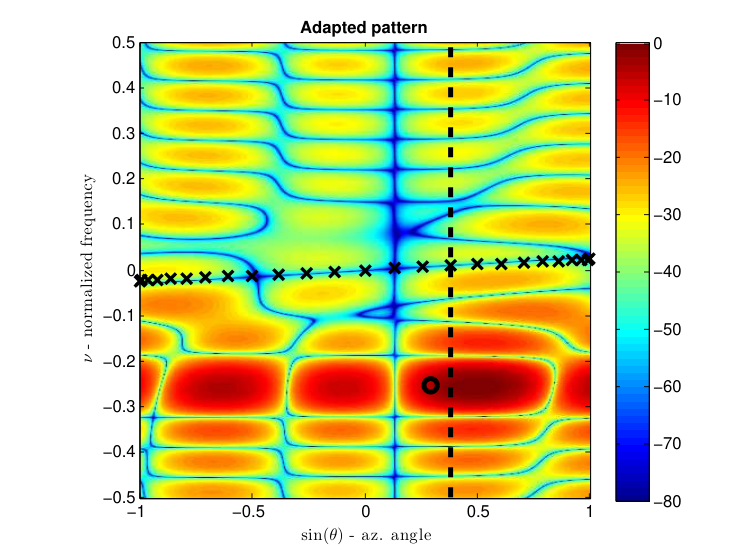
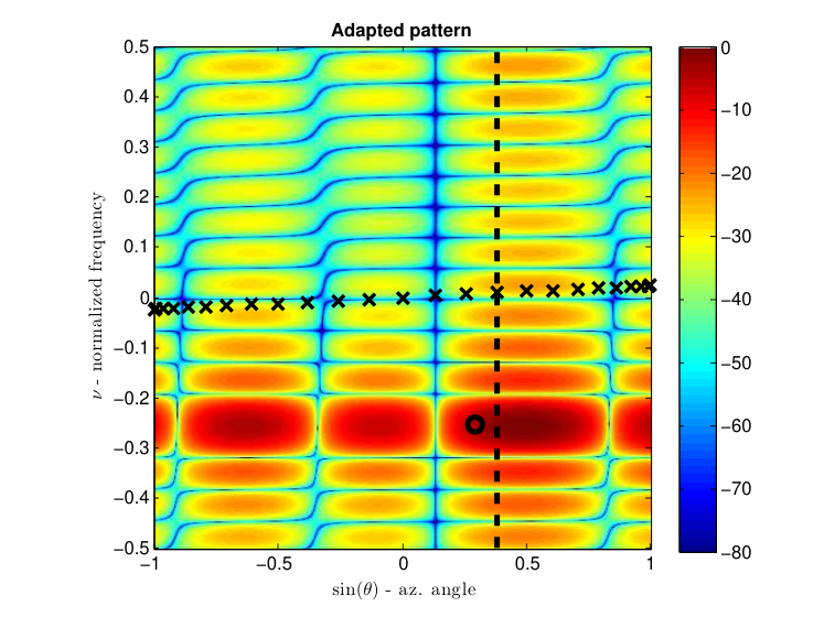
Refer to caption
Fig. 33: Adapted Pattern (dB relative to peak), QuadSolver. Target at ○\bigcirc, Clutter phase centers at ×\times, Interferer (dashed line) at (θ,ϕ)=(0.3941,0.3)(\theta,\phi)=(0.3941,0.3) radians
Refer to caption
Fig. 34: Adapted Pattern, NormSolver. Target at ○\bigcirc, Clutter phase centers at ×\times, Interferer (dashed line) at (θ,ϕ)=(0.3941,0.3)(\theta,\phi)=(0.3941,0.3)

For completeness, we also show the adapted pattern cuts under the interference scenario. Again, in all figures, the dashed line represents the target location. Figures 35 and 36 show the cut along the target Doppler. The significant bias seen above is more clear here, which would result in a rather large angle estimation error.

Fig. 35: Adapted Pattern (dB scale), cut at target Doppler, QuadSolver. Interference.
Fig. 36: Adapted Pattern (dB scale), cut at target Doppler, NormSolver. Interference.

The cuts along the target azimuth, shown in Figures 37 and 38, still appropriately localize the target in some sense. However, note that in both cases, the peak gain at the target Doppler has dropped about 5 dB from the gain in Figures 31 and 32. Thus, there is a clear loss in both dimensions due to the interferer.

Fig. 37: Adapted Pattern (dB scale), cut at target azimuth, QuadSolver. Interference.
Fig. 38: Adapted Pattern (dB scale), cut at target azimuth, NormSolver. Interference.

We note that this interference impact (in all cases) is lessened by increasing MM in our simulations. This is not surprising, since more antenna elements over the same aperture increases the degrees of freedom available to null interference and localize the target.

VIII Conclusions

In this report, we reconsidered the problem of [1] under the relaxed biquadratic program framework. We demonstrated definitively that the problem is non-convex, then showed the relaxation process. We then showed that the KKTs require power-bounded solutions when the noise-and-interference matrix is full rank, and that such a solution admits a waterfilling interpretation. Simulations demonstrated that numerical solvers can provide divergent solution paths, depending on scaling – one closer to the traditional clutter-nulling process, the other relying on a matched target-in-clutter response. Future work will attempt to generalize the findings made in this report and demonstrate its utility for other radar system models that admit a channel response representation.

References

  • [1] P. Setlur and M. Rangaswamy, “Waveform design for radar STAP in signal dependent interference,” IEEE Transactions on Signal Processing, vol. 64, no. 1, pp. 19–34, January 2016.
  • [2] N. L. Owsley, “A recent trend in adaptive spatial processing for sensor arrays: Constrained adaptation,” in Signal Processing, J. W. R. Griffiths, P. L. Stocklin, and C. van Schoonfeld, Eds. Academic Press, 1972, pp. 591–604.
  • [3] R. Klemm, Principles of Space-Time Adaptive Processing. Institution of Electrical Engineers, 2002.
  • [4] J. Ward, “Space-time adaptive processing for airborne radar,” Massachusetts Institute of Technology, Lincoln Laboratory, Tech. Rep., 1994.
  • [5] D. Madurasinghe and A. P. Shaw, “Mainlobe jammer nulling via TSI finders: a space-time adaptive processor,” EURASIP Journal on Applied Signal Processing, vol. 2006, pp. 1–13, 2006.
  • [6] Y. Seliktar, D. B. Williams, and E. J. Holder, “A space/fast-time adaptive monopulse technique,” EURASIP Journal on Applied Signal Processing, vol. 2006, pp. 1–11, 2006.
  • [7] J. Capon, “High-resolution frequency-wavenumber spectrum analysis,” Proceedings of the IEEE, vol. 57, no. 8, pp. 1408–1418, January 1969.
  • [8] A. Aubry, A. DeMaio, M. Piezzo, A. Farina, and M. Wicks, “Cognitive design of the receive filter and transmitted phase code in reverberating environment,” IET Radar, Sonar and Navigation, vol. 6, no. 9, pp. 822–833, December 2012, barf 1.
  • [9] A. Aubry, A. DeMaio, A. Farina, and M. Wicks, “Knowledge-aided (potentially cognitive) transmit signal and receive filter design in signal-dependent clutter,” IEEE Transactions on Aerospace and Electronic Systems, vol. 49, no. 1, pp. 93–117, January 2013.
  • [10] C. Y. Chen and P. P. Vaidyanathan, “MIMO radar waveform optimization with prior information of the extended target and clutter,” IEEE Transactions on Signal Processing, vol. 57, no. 9, pp. 3533–3544, 2009.
  • [11] P. Stoica, H. He, and J. Li, “Optimization of the receive filter and transmit sequence for active sensing,” IEEE Trans. Signal Processing, vol. 60, no. 4, pp. 1730–1740, April 2012.
  • [12] S. Boyd and L. Vandenberghe, Convex Optimization. New York, NY, USA: Cambridge University Press, 2004.
  • [13] C. Ling, J. Nie, L. Qi, and Y. Ye, “Biquadratic optimization over unit spheres and semidefinite programming relaxations,” SIAM Journal of Optimization, vol. 20, pp. 1286–1310, 2009.
  • [14] C. Ling, X. Zhang, and L. Qi, “Semidefinite relaxation approximation for multivariate bi-quadratic optimization with quadratic constraints,” Numer. Linear Algebra Appl., vol. 19, no. 1, pp. 113–131, apr 2011. [Online]. Available: http://dx.doi.org/10.1002/nla.781
  • [15] J. R. Magnus and H. Neudecker, “The Commutation Matrix: Some Properties and Applications,” The Annals of Statistics, vol. 7, no. 2, pp. 381–394, Mar. 1979.
  • [16] J. R. Guerci, J. S. Bergin, R. J. Guerci, M. Khanin, and M. Rangaswamy, “A new mimo clutter model for cognitive radar,” in 2016 IEEE Radar Conference (RadarConf), May 2016, pp. 1–6.
  • [17] A. Hjørungnes, Complex-Valued Matrix Derivatives, 1st ed. Cambridge, UK: Cambridge University Press, 2011.
  • [18] G. A. F. Seber, A Matrix Handbook for Statisticians, 1st ed. Hoboken, NJ, USA: John Wiley & Sons, Inc., Nov. 2007.
  • [19] E. Kreindler and A. Jameson, “Conditions for nonnegativeness of partitioned matrices,” IEEE Trans. Automat. Contr., vol. 17, no. 1, pp. 147–148, Feb. 1972.
  • [20] R. A. Horn and C. R. Johnson, Matrix Analysis, 2nd ed. New York, NY: Cambridge University Press, 2013.
  • [21] I. M. Bomze, C. Ling, L. Qi, and X. Zhang, “Standard bi-quadratic optimization problems and unconstrained polynomial reformulations,” J. Glob. Optim., vol. 52, no. 4, pp. 663–687, 2012. [Online]. Available: http://dx.doi.org/10.1007/s10898-011-9710-5
  • [22] X. Zhang, C. Ling, and L. Qi, “Semidefinite relaxation bounds for bi-quadratic optimization problems with quadratic constraints,” J. Glob. Optim., vol. 49, pp. 293–311, 2011.
  • [23] C. G. Khatri and S. K. Mitra, “Hermitian and nonnegative definite solutions of linear matrix equations,” SIAM Journal on Applied Mathematics, vol. 31, no. 4, pp. 579–7, 12 1976, copyright - Copyright] © 1976 Society for Industrial and Applied Mathematics; Last updated - 2012-01-24. [Online]. Available: http://search.proquest.com.wrs.idm.oclc.org/docview/917326738?accountid=26189
  • [24] J. K. Baksalary, “Nonnegative definite and positive definite solutions to the matrix equation axa* = b,” Linear and Multilinear Algebra, vol. 16, no. 1-4, pp. 133–139, 1984. [Online]. Available: http://dx.doi.org/10.1080/03081088408817616
  • [25] L. E. Brennan and F. M. Staudaher, “Subclutter visibility demonstration,” Adaptive Sensors Incorporated, Tech. Rep. RL-TR-92-21, March 1992.
  • [26] N. A. Goodman and J. M. Stiles, “On clutter rank observed by arbitrary arrays,” IEEE Trans. Signal Processing, vol. 55, no. 1, pp. 178 – 186, January 2007.
  • [27] P. Setlur, N. Devroye, and M. Rangaswamy, “Radar waveform design with the two step mutual information,” in 2014 IEEE Radar Conference, May 2014, pp. 1317–1322.
  • [28] M. Grant and S. Boyd, “CVX: Matlab software for disciplined convex programming, version 2.1,” http://cvxr.com/cvx, June 2015.
  • [29] ——, “Graph implementations for nonsmooth convex programs,” in Recent Advances in Learning and Control, ser. Lecture Notes in Control and Information Sciences, V. Blondel, S. Boyd, and H. Kimura, Eds. Springer-Verlag Limited, 2008, pp. 95–110, http://stanford.edu/ boyd/graph_dcp.html.
  • [30] K. Toh, M. Todd, and R. Tutuncu, “SDPT3 — a matlab software package for semidefinite programming,” Optimization Methods and Software, vol. 11, pp. 545–581, 1999.
  • [31] R. Tutuncu, K. Toh, and M. Todd, “Solving semidefinite-linear-quadratic programs using SDPT3,” Mathematical Programming Ser. B, vol. 95, pp. 189–217, 2003.