August 2016 \phd\deptComputer Science and Automation \facultyFaculty of Engineering
Resolving the Complexity of Some Fundamental Problems in Computational Social Choice
© Palash Dey
August 2016
All rights reserved
DEDICATED TO
My teachers
Acknowledgements I am grateful to my Ph.D. advisors Prof. Y. Narahari and Prof. Arnab Bhattacharyya for providing me a golden opportunity to work with them. I thank them for the all encompassing support they ushered upon me throughout my Ph.D. I convey my special thanks to Prof. Y. Narahari for all his academic and nonacademic supports which made my Ph.D. life very easy and enjoyable. I have throughly enjoyed working with Prof. Arnab Bhattacharyya. I convey my very special thanks to Prof. Neeldhara Misra for many excellent and successful research collaborations, useful discussions, and playing an all encompassing super-active role in my Ph.D. life. Prof. Neeldhara Misra was always my constant source of inspiration and she guided me throughout my Ph.D. as a supervisor, advisor, friend, and elder sister. I am indebted to Prof. Dilip P. Patil for teaching me how the practice of writing statements rigorously and precisely in mathematics automatically clarifies many doubts. I am extremely grateful to have a teacher like him at the very early stage of my stay in IISc who not only significantly improved my mathematical thinking process but also acted like a friend, philosopher, and guide throughout my stay in IISc. I throughly enjoyed all the courses that he taught during my stay in IISc and learned a lot from those courses. Specially his courses on linear algebra, Galois theory, commutative algebra have immensely influenced my thinking process.
I thank Prof. Sunil Chandran for teaching me the art of proving results in graph theory in particular and theoretical computer science in general. I am grateful to Dr. Deeparnab Chakrabarty and Prof. Arnab Bhattacharyya for teaching me approximation algorithms and randomized algorithms, Prof. Manjunath Krishnapur for teaching me probability theory and martingales, Prof. Chandan Saha for teaching me complexity theory and algebraic geometry, Prof. Y. Narahari for teaching me game theory. I thank all the faculty members of Department of Computer Science and Automation (CSA) for all of their supports. I convey my special thank to all the staffs of CSA specially Ms. Suguna, Ms. Meenakshi, Ms. Kushael for their helping hands. I thank Prof. Ashish Goel for giving me an excellent opportunity to work with him and for hosting me in Stanford University for three months. I thank Dr. David Woodruff for collaborating with me on important problems.
I feel myself extremely lucky to get such a wonderful and friendly lab members in the Game Theory lab. I want to thank all the members of the Game Theory lab with special mention to Dr. Rohith D. Vallam, Satyanath Bhat, Ganesh Ghalme, Shweta Jain, Swapnil Dhamal, Divya Padmanabhan, Dr. Pankaj Dayama, Praful Chandra, Shourya Roy, Tirumala Nathan, Debmalya Mandal, Arupratan Ray, and Arpita Biswas. I want to thank Dr. Minati De, Abhiruk Lahiri, Achintya Kundu, Aniket Basu Roy, Prabhu Chandran, Prasenjit Karmakar, R Kabaleeshwaran, Rohit Vaish, Sayantan Mukherjee, Srinivas Karthik, Suprovat Ghoshal, Vineet Nair for all the important discussions. I greatly acknowledge support from Ratul Ray and Uddipta Maity during my internship in Stanford University.
I thank Google India for providing me fellowship during second and third years of my Ph.D. I acknowledge financial support from Ministry of Human Resource Development (MHRD) in India during my first year of Ph.D.
Last but not the least, I express my gratitude to my parents, brother, wife, and all my friends for their love, blessing, encouragement, and support. \prefacesectionAbstract In many real world situations, especially involving multiagent systems and artificial intelligence, participating agents often need to agree upon a common alternative even if they have differing preferences over the available alternatives. Voting is one of the tools of choice in these situations. Common and classic applications of voting in modern applications include collaborative filtering and recommender systems, metasearch engines, coordination and planning among multiple automated agents etc. Agents in these applications usually have computational power at their disposal. This makes the study of computational aspects of voting crucial. This thesis is devoted to a study of computational complexity of several fundamental algorithmic and complexity-theoretic problems arising in the context of voting theory.
The typical setting for our work is an “election”; an election consists of a set of voters or agents, a set of alternatives, and a voting rule. The vote of any agent can be thought of as a ranking (more precisely, a complete order) of the set of alternatives. A voting profile comprises a collection of votes of all the agents. Finally, a voting rule is a mapping that takes as input a voting profile and outputs an alternative, which is called the “winner” or “outcome” of the election. Our contributions in this thesis can be categorized into three parts and are described below.
Part I: Preference Elicitation.
In the first part of the thesis, we study the problem of eliciting the preferences of a set of voters by asking a small number of comparison queries (such as who a voter prefers between two given alternatives) for various interesting domains of preferences.
We commence with considering the domain of single peaked preferences on trees in Chapter 3. This domain is a significant generalization of the classical well studied domain of single peaked preferences. The domain of single peaked preferences and its generalizations are hugely popular among political and social scientists. We show tight dependencies between query complexity of preference elicitation and various parameters of the single peaked tree, for example, number of leaves, diameter, path width, maximum degree of a node etc.
We next consider preference elicitation for the domain of single crossing preference profiles in Chapter 4. This domain has also been studied extensively by political scientists, social choice theorists, and computer scientists. We establish that the query complexity of preference elicitation in this domain crucially depends on how the votes are accessed and on whether or not any single crossing ordering is a priori known.
Part II: Winner Determination.
In the second part of the thesis, we undertake a study of the computational complexity of several important problems related to determining winner of an election.
We begin with a study of the following problem: Given an election, predict the winner of the election under some fixed voting rule by sampling as few votes as possible. We establish optimal or almost optimal bounds on the number of votes that one needs to sample for many commonly used voting rules when the margin of victory is at least ( is the number of voters and is a parameter). We next study efficient sampling based algorithms for estimating the margin of victory of a given election for many common voting rules. The margin of victory of an election is a useful measure that captures the robustness of an election outcome. The above two works are presented in Chapter 5.
In Chapter 6, we design an optimal algorithm for determining the plurality winner of an election when the votes are arriving one-by-one in a streaming fashion. This resolves an intriguing question on finding heavy hitters in a stream of items, that has remained open for more than years in the data stream literature. We also provide near optimal algorithms for determining the winner of a stream of votes for other popular voting rules, for example, veto, Borda, maximin etc.
Voters’ preferences are often partial orders instead of complete orders. This is known as the incomplete information setting in computational social choice theory. In an incomplete information setting, an extension of the winner determination problem which has been studied extensively is the problem of determining possible winners. We study the kernelization complexity (under the complexity-theoretic framework of parameterized complexity) of the possible winner problem in Chapter 7. We show that there do not exist kernels of size that is polynomial in the number of alternatives for this problem for commonly used voting rules under a plausible complexity theoretic assumption. However, we also show that the problem of coalitional manipulation which is an important special case of the possible winner problem admits a kernel whose size is polynomially bounded in the number of alternatives for common voting rules.
Part III: Election Control.
In the final part of the thesis, we study the computational complexity of various interesting aspects of strategic behavior in voting.
First, we consider the impact of partial information in the context of strategic manipulation in Chapter 8. We show that lack of complete information makes the computational problem of manipulation intractable for many commonly used voting rules.
In Chapter 9, we initiate the study of the computational problem of detecting possible instances of election manipulation. We show that detecting manipulation may be computationally easy under certain scenarios even when manipulation is intractable.
The computational problem of bribery is an extensively studied problem in computational social choice theory. We study computational complexity of bribery when the briber is “frugal” in nature. We show for many common voting rules that the bribery problem remains intractable even when the briber’s behavior is restricted to be frugal, thereby strengthening the intractability results from the literature. This forms the subject of Chapter 10.
Publications based on this Thesis
- 1.
Palash Dey, Neeldhara Misra, and Yadati Narahari. “Kernelization Complexity of Possible Winner and Coalitional Manipulation Problems in Voting”. In Theoretical Computer Science, volume 616, pages 111-125, February 2016.
Remark: A preliminary version of this work was presented in the International Conference on Autonomous Systems and Multiagent Systems (AAMAS-15), 2015. - 2.
Palash Dey, Neeldhara Misra, and Yadati Narahari. “Frugal Bribery in Voting”. Accepted in Theoretical Computer Science, March 2017.
Remark: A preliminary version of this work was presented in the AAAI Conference on Artificial Intelligence (AAAI-16), 2016. - 3.
Arnab Bhattacharyya, Palash Dey, and David P. Woodruff. “An Optimal Algorithm for -Heavy Hitters in Insertion Streams and Related Problems”. Proceedings of the ACM SIGMOD-SIGACT-SIGAI Symposium on Principles of Database Systems (PODS-16), pages 385-400, San Francisco, USA, 26 June - 1 July, 2016.
- 4.
Palash Dey and Neeldhara Misra. “Elicitation for Preferences Single Peaked on Trees”. Proceedings of the International Joint Conference on Artificial Intelligence (IJCAI-16), pages 215-221, New York, USA, 9-15 July, 2016.
- 5.
Palash Dey and Neeldhara Misra. “Preference Elicitation For Single Crossing Domain”. Proceedings of the International Joint Conference on Artificial Intelligence (IJCAI-16), pages 222-228, New York, USA, 9-15 July, 2016.
- 6.
Palash Dey, Neeldhara Misra, and Yadati Narahari. “Complexity of Manipulation with Partial Information in Voting”. Proceedings of the International Joint Conference on Artificial Intelligence (IJCAI-16), pages 229-235, New York, USA, 9-15 July, 2016.
- 7.
Palash Dey, Neeldhara Misra, and Yadati Narahari. “Frugal Bribery in Voting”. Proceedings of the AAAI Conference on Artificial Intelligence (AAAI-16), vol. 4, pages 2466-2672, Phoenix, Arizona, USA, 2016.
- 8.
Palash Dey and Yadati Narahari. “Estimating the Margin of Victory of Elections using Sampling”. Proceedings of the International Joint Conference on Artificial Intelligence (IJCAI-15), pages 1120-1126, Buenos Aires, Argentina, 2015.
- 9.
Palash Dey and Arnab Bhattacharyya. “Sample Complexity for Winner Prediction in Elections”. Proceedings of the International Conference on Autonomous Systems and Multiagent Systems (AAMAS-15), pages 1421-1430, Istanbul, Turkey, 2015.
- 10.
Palash Dey, Neeldhara Misra, and Yadati Narahari. “Detecting Possible Manipulators in Elections”. Proceedings of the International Conference on Autonomous Systems and Multiagent Systems(AAMAS-15), pages 1441-1450, Istanbul, Turkey, 2015.
- 11.
Palash Dey, Neeldhara Misra, and Yadati Narahari “Kernelization Complexity of Possible Winner and Coalitional Manipulation Problems in Voting”. Proceedings of the International Conference on Autonomous Systems and Multiagent Systems (AAMAS-15), pages 87-96, Istanbul, Turkey, 2015.
Chapter 1 Introduction
In this chapter, we provide an informal introduction to the area called social choice theory and motivate its computational aspects. We then provide an overview of the thesis along with further motivations for the problems we study in this thesis.
People always have different opinions on almost everything and hence they often have to come to a decision collectively on things that affect all of them. There are various ways for people with different opinions to come to a decision and the use of voting is the most natural and common method for this task. Indeed, the use of voting can be traced back to Socrates (470-399 BC) who was sentenced to death by taking a majority vote. We also see the mention of voting rules in Plato’s (424-348 BC) unfinished book “Laws”. Then, in the Middle Ages, the Catalan philosopher, poet, and missionary Ramon Llull (1232-1316) mentioned Llull voting in his manuscripts Ars notandi, Ars eleccionis, and Alia ars eleccionis, which were lost until 2001. The German philosopher, theologian, jurist, and astronomer Nicholas of Cusa (1401-1464) suggested the method for electing the Holy Roman Emperor in 1433. The first systematic study of the theory of voting was carried out by two French mathematicians, political scientists, and philosophers Marie Jean Antoine Nicolas de Caritat, marquis de Condorcet (1743-1794) and Jean-Charles, chevalier de Borda (1733-1799). A more involved study of voting was pioneered by Kenneth Arrow (a co-recipient of the Nobel Memorial Prize in Economics in 1972). The celebrated Arrow’s impossibility theorem in 1951 along with Gibbard-Satterthwaite’s impossibility theorem in 1973 and 1977 laid the foundation stone of modern voting theory.
1.1 Important Aspects of Voting
In a typical setting for voting, we have a set of alternatives or candidates, a set of agents called voters each of whom has an ordinal preference called votes over the candidates, and a voting rule which chooses one or a set of candidates as winner(s). We call a set of voters along with their preferences over a set of candidates and a voting rule an election. In Table 1.1 we exhibit an election with a set of voters {Satya, Shweta, Swapnil, Divya, Ganesh} and a set of five ice cream flavors {Chocolate, Butterscotch, Pesta, Vanilla, Kulfi} as a set of candidates. Suppose we use the plurality voting rule which chooses the candidate that is placed at the first positions of the votes most often as winner. Then the winner of the plurality election in Table 1.1 is Chocolate. Plurality voting rule is among the simplest voting rules and only observes the first position of every vote to determine the winner. Mainly due to its simplicity, the plurality voting rule frequently finds its applications in voting scenarios where human beings are involved, for example, political elections. Indeed many countries including India, Singapore, United Kingdom, Canada use plurality voting at various levels of elections [201].
| Voters | Preferences |
| Satya | Chocolate Kulfi Butterscotch Vanilla Pesta |
| Shweta | Butterscotch Kulfi Chocolate Vanilla Pesta |
| Swapnil | Pesta Butterscotch Kulfi Vanilla Chocolate |
| Divya | Chocolate Vanilla Kulfi Pesta Butterscotch |
| Ganesh | Kulfi Butterscotch Chocolate Vanilla Pesta |
However, there are more sophisticated voting rules which takes into account the entire preference ordering of the voters to choose a winner. One such voting rule which finds its widespread use specially in sports and elections in many educational institutions is the Borda voting rule [35]. The Borda voting rule, first proposed by Jean-Charles, chevalier de Borda in 1770, gives a candidate a score equal to the number of other candidates it is preferred over for every vote. In Table 1.1 for example, the candidate Kulfi receives a score of 3 from Satya, 3 from Shweta, 2 from Swapnil, 2 from Divya, and 4 from Ganesh. Hence the Borda score of Kulfi is 14. It can be verified that the Borda score of every other candidate is less than 14 which makes Kulfi the Borda winner of the election. We can already observe how two widely used and intuitively appealing voting rules select two different winners for the same set of votes.
A closer inspection of Table 1.1 reveals something peculiar about what the plurality and Borda voting rules choose as winners. The plurality voting rule chooses Chocolate as the winner whereas a majority (three out of five) of the voters prefer Butterscotch over Chocolate. The same phenomenon is true for the Borda winner (Kulfi) too — a majority of the voters prefer Butterscotch over Kulfi. More importantly Butterscotch is preferred over every other alternative (ice cream flavors) by a majority of the voters. Such an alternative, if it exists, which is preferred over every other alternative by a majority of the voters, is called the Condorcet winner of the election, named after the French mathematician and philosopher Marie Jean Antoine Nicolas de Caritat, marquis de Condorcet. We provide a more detailed discussion to all these aspects of voting including others in Chapter 2.
Now let us again consider the example in Table 1.1. Suppose Shweta misreports her preference as “Butterscotch Pesta Chocolate Vanilla Kulfi.” Observe that the misreported vote of Shweta when tallied with the other votes makes Butterscotch the Borda winner with a Borda score of 12. Moreover, misreporting her preference results in an outcome (that is Butterscotch) which Shweta prefers over the honest one (that is Kulfi). This example demonstrate a fundamental notion in voting theory called manipulation — there can be instances where an individual voter may have an outcome by misreporting her preference which she prefers over the outcome of honest voting (according to her preference). Obviously manipulation is undesirable since it leads to suboptimal societal outcome. Hence one would like to use voting rules that do not create such possibilities of manipulation. Such voting rules are called strategy-proof voting rules. When we have only two candidates, it is known that the majority voting rule, which selects the majority candidate (breaking ties arbitrarily) as the winner, is a strategy-proof voting rule. There exist strategy-proof voting rules even if we have more than two candidates. For example, consider the voting rule that always outputs the candidate which is preferred most by some fixed voter say . Obviously is strategy-proof since any voter other than cannot manipulate simply because they can never change the outcome of the election and the winner is already the most preferred candidate of . However, voting rules like are undesirable intuitively because it is not performing the basic job of voting which is aggregating preferences of all the voters. The voting rule is called a dictatorship since it always selects the candidate preferred most by some fixed voter ; such a voter is called a dictator. Hence an important question to ask is the following: do there exist voting rules other than dictatorship that are strategy-proof with more than two candidates? Unfortunately classical results in social choice theory by Gibbard and Satterthwaite prove that there does not exist any such onto voting rule [124, 213] if we have more than two candidates. A voting rule is onto if every candidate is selected for some set of votes. We formally introduce all these fundamental aspects of voting including others in Chapter 2.
1.2 Applications and Challenges of Voting Theory Relevant to Computer Science
With rapid improvement of computational power, the theory of voting found its applications not only in decision making among human beings but also in aggregating opinions of computational agents. Indeed, voting is commonly used whenever any system with multiple autonomous agents wish to take a common decision. Common and classic applications of voting in multiagent systems in particular and artificial intelligence in general include collaborative filtering and recommender systems [200], planning among multiple automated agents [104], metasearch engines [74], spam detection [66], computational biology [145], winner determination in sports competitions [12], similarity search and classification of high dimensional data [116]. The extensive use of voting by computational agents makes the study of computational aspects of voting extremely important. In many applications of voting in artificial intelligence, one often has a huge number of voters and candidates. For example, voting has been applied in the design of metasearch engines [74] where the number of alternatives the agents are voting for is in the order of trillions if not more — the alternatives are the set of web pages in this case. In a commercial recommender system, for example Amazon.com, we often have a few hundred millions of users and items. In these applications, we need computationally efficient algorithms for quickly finding a winner of an election with so many candidates and voters.
Moreover, the very fact that the agents now have computational power at their disposal allows them to easily strategize their behavior instead of acting truthfully. For example, the problem of manipulation is much more severe in the presence of computational agents since the voters can easily use their computational power to find a manipulative vote. The field known as computational social choice theory (COMSOC) studies various computational aspects in the context of voting. We refer the interested readers to a recent book on computational social choice theory for a more elaborate exposition [165].
Other than practical applications, the theory of voting turns out to be crucial in proving various fundamental theoretical results in computer science. Indeed, a notion known as noise stability of majority voting has been beautifully utilized for proving a lower bound on the quality of any polynomial time computable approximate solution of the maximum cut problem in a undirected graph [147, 176]. We refer interested reader to [195] for a more detailed discussion.
1.3 Thesis Overview
In this thesis, we resolve computational questions of several fundamental problems arising in the context of voting theory. We provide a schematic diagram of the contribution of the thesis in Figure 1.1. We begin our study with the first step in any election system – eliciting the preferences of the voters. We consider the problem of preference elicitation in the first part of the thesis and develop (often) optimal algorithms for learning the preferences of a set of voters. In the second part of the thesis, we develop (often) optimal sublinear time algorithms for finding the winner of an election. The problem of determining winner of an election is arguably the most fundamental problem that comes to our mind once the preferences of all the voters have been elicited. In the third part of the thesis, we exhibit complexity-theoretic results for various strategic aspects of voting.
1.3.1 Part I: Preference Elicitation
The first step in any election system is to receive preferences of the voters as input. However, it may often be impractical to simply ask the voters for their preferences due to the presence of a huge number of alternatives. For example, asking users of Amazon.com to provide a complete ranking of all the items does not make sense. In such scenarios, one convenient way to know these agents’ preferences is to ask the agents to compare (a manageable number of) pairs of items. However, due to the existence of a strong query complexity lower bound (from sorting), we can hope to reduce the burden of eliciting preference from the agents only by assuming additional structure on the preferences. Indeed, in several application scenarios commonly considered, it is rare that preferences are entirely arbitrary, demonstrating no patterns whatsoever. For example, the notion of single peaked preferences forms the basis of several studies in the analytical political sciences. Intuitively, preferences of a set of agents is single peaked if the alternatives and the agents can be arranged in a linear order and the preferences “respect” this order. We defer the formal definition of single peaked profiles to Chapter 3.
We show in Chapters 3 and 4 that the query complexity for preference elicitation can be reduced substantially by assuming practically appealing restrictions on the domain of the preferences.
Chapter 3: Preference Elicitation for Single Peaked Preferences on Trees
Suppose we have agents and alternatives. Then it is known that if the preferences are single peaked, then elicitation can be done using comparisons [54]. The notion of single peaked preferences has been generalized to single peaked preferences in a tree — intuitively, the preferences should be single peaked on every path of the tree. We show that if the single peaked tree has leaves, then elicitation can be done using comparisons [82]. We also show that other natural parameters of the single peaked tree, for example, its diameter, path width, minimum degree, maximum degree do not decide the query complexity for preference elicitation.
Chapter 4: Preference Elicitation for Single Crossing Preferences
Another well studied domain is the domain of single crossing profiles. Intuitively, a set of preferences is single crossing if the preferences can be arranged in a linear order such that all the preferences who prefer an alternative over another alternative are consecutive, for every and . We consider in [83] two distinct scenarios: when an ordering of the voters with respect to which the profile is single crossing is known a priori versus when it is unknown. We also consider two different access models: when the votes can be accessed at random, as opposed to when they arise in any arbitrary sequence. In the sequential access model, we distinguish two cases when the ordering is known: the first is that the sequence in which the votes appear is also a single-crossing order, versus when it is not. The main contribution of our work is to provide polynomial time algorithms with low query complexity for preference elicitation in all the above six cases. Further, we show that the query complexities of our algorithms are optimal up to constant factor for all but one of the above six cases.
1.3.2 Part II: Winner Determination
Once we have elicited the preferences of the voters, the next important task in an election is to determine the winner of this election. We show interesting complexity theoretic results on determining the winner of an election under a variety of application scenarios.
Chapter 5: Winner Prediction
We begin by studying the following problem: Given an election, predict the winner of the election under some fixed voting rule by sampling as few preferences as possible. Our results show that the winner of an election can be determined (with high probability) by observing only a few preferences that are picked uniformly at random from the set of preferences. We show this result for many common voting rules when the margin of victory is at least [69], where is the number of voters and is a parameter. The margin of victory of an election is the smallest number of preferences that must be modified to change the winner of an election. We also establish optimality (in terms of the number of preferences our algorithms sample) of most of our algorithms by proving tight lower bounds on the sample complexity of this problem.
Another important aspect of an election is the robustness of the election outcome. A popular measure of robustness of an election outcome is its margin of victory. We develop efficient sampling based algorithms for estimating the margin of victory of a given election for many common voting rules [92]. We also show optimality of our algorithms for most of the cases under appealing practical scenarios.
Chapter 6: Winner Determination in Streaming
An important, realistic model of data in big data research is the streaming model. In the setting that we consider, the algorithms are allowed only one pass over the data. We give the first optimal bounds for returning the -heavy hitters in an insertion only data stream, together with their approximate frequencies, thus settling a long line of work on this problem. For a stream of items in and parameters , let denote the frequency of item , i.e., the number of times item occurs in the stream in [20]. With arbitrarily large constant probability, our algorithm returns all items for which , returns no items for which , and returns approximations with for each item that it returns. Our algorithm uses bits of space, processes each stream update in worst-case time, and can report its output in time linear in the output size. We also prove a lower bound, which implies that our algorithm is optimal up to a constant factor in its space complexity. A modification of our algorithm can be used to estimate the maximum frequency up to an additive error in the above amount of space, resolving an open question on algorithms for data streams for the case of -heavy hitters. We also introduce several variants of the heavy hitters and maximum frequency problems, inspired by rank aggregation and voting schemes, and show how our techniques can be applied in such settings. Unlike the traditional heavy hitters problem, some of these variants look at comparisons between items rather than numerical values to determine the frequency of an item.
Chapter 7: Kernelization Complexity for Determining Possible Winners
Voters’ preferences are often partial orders instead of complete orders. This is known as the incomplete information setting in computational social choice theory. In an incomplete information setting, an extension of the winner determination problem which has been studied extensively is the problem of determining possible winners. An alternative is a possible winner in a set of incomplete preferences if there exists a completion of these incomplete preferences where the alternative wins. Previous work has provided, for many common voting rules, fixed parameter tractable algorithms for the Possible winner problem, with number of candidates as the parameter. However, the corresponding kernelization question is still open, and in fact, has been mentioned as a key research challenge [14]. In this work, we settle this open question for many common voting rules.
We show in [85, 88] that the Possible winner problem for maximin, Copeland, Bucklin, ranked pairs, and a class of scoring rules that includes the Borda voting rule do not admit a polynomial kernel with the number of candidates as the parameter. We show however that the Coalitional manipulation problem which is an important special case of the Possible winner problem does admit a polynomial kernel for maximin, Copeland, ranked pairs, and a class of scoring rules that includes the Borda voting rule, when the number of manipulators is polynomial in the number of candidates. A significant conclusion of this work is that the Possible winner problem is computationally harder than the Coalitional manipulation problem since the Coalitional manipulation problem admits a polynomial kernel whereas the Possible winner problem does not admit a polynomial kernel.
1.3.3 Part III: Election Control
When agents in a multiagent system have conflicting goals, they can behave strategically to make the system produce an outcome that they favor. For example, in the context of voting, there can be instances where an agent, by misreporting her preference, can cause the election to result in an alternative which she prefers more than the alternative that would have been the outcome in case she had reported her preference truthfully. This phenomenon is called manipulation. Certainly, we would like to design systems that are robust to such manipulation. Unfortunately, classical results in social choice theory establish that any reasonable voting rule will inevitably create such opportunities for manipulation. In this context, computer scientists provide some hope by showing that the computational problem of manipulation can often be intractable. Indeed, if a computationally bounded agent has to solve an intractable problem to manipulate the election system, then the agent would, in all likelihood, fail to manipulate.
Chapter 8: Manipulation with Partial Information
The computational problem of manipulation has classically been studied in a complete information setting – the manipulators know the preference of every other voter. We extend this line of work to the more practical, incomplete information setting where agents have only a partial knowledge about the preferences of other voters [86]. In our framework, the manipulators know a partial order for each voter that is consistent with the true preference of that voter. We say that an extension of a partial order is viable if there exists a manipulative vote for that extension. We propose the following notions of manipulation when manipulators have incomplete information about the votes of other voters.
- 1.
Weak Manipulation: the manipulators seek to vote in a way that makes their preferred candidate win in at least one extension of the partial votes of the non-manipulators.
- 2.
Opportunistic Manipulation: the manipulators seek to vote in a way that makes their preferred candidate win in every viable extension of the partial votes of the non-manipulators.
- 3.
Strong Manipulation: the manipulators seek to vote in a way that makes their preferred candidate win in every extension of the partial votes of the non-manipulators.
We consider several scenarios for which the traditional manipulation problems are easy (for instance, the Borda voting rule with a single manipulator). For many of them, the corresponding manipulative questions that we propose turn out to be computationally intractable. Our hardness results often hold even when very little information is missing, or in other words, even when the instances are very close to the complete information setting. Our overall conclusion is that computational hardness continues to be a valid obstruction or deterrent to manipulation, in the context of the more realistic setting of incomplete information.
Chapter 9: Manipulation Detection
Even if the computational problem of manipulation is almost always intractable, there have been many instances of manipulation in real elections. In this work, we initiate the study of the computational problem of detecting possible instances of manipulation in an election [84]. We formulate two pertinent computational problems in the context of manipulation detection - Coalitional Possible Manipulators (CPM) and Coalitional Possible Manipulators given Winner (CPMW), where a suspect group of voters is provided as input and we have to determine whether they can form a potential coalition of manipulators. In the absence of any suspect group, we formulate two more computational problems namely Coalitional Possible Manipulators Search (CPMS) and Coalitional Possible Manipulators Search given Winner (CPMSW). We provide polynomial time algorithms for these problems, for several popular voting rules. For a few other voting rules, we show that these problems are NP-complete. We observe that detecting possible instances of manipulation may be easy even when the actual manipulation problem is computationally intractable, as seen for example, in the case of the Borda voting rule.
Chapter 10: Frugal Bribery
Another fundamental problem in the context of social choice theory is bribery. Formally, the computational problem of bribery is as follows: given (i) a set of votes, (ii) a cost model for changing the votes, (iii) a budget, and (iv) a candidate , is it possible for an external agent to bribe the voters to change their votes (subject to the budget constraint) so that wins the election? We introduce and study two important special cases of the classical $Bribery problem, namely, Frugal-bribery and Frugal-$bribery where the briber is frugal in nature in [87]. By this, we mean that the briber is only able to influence voters who benefit from the suggestion of the briber. More formally, a voter is vulnerable if the outcome of the election improves according to her own preference when she accepts the suggestion of the briber. In the Frugal-bribery problem, the goal of the briber is to make a certain candidate win the election by changing only the vulnerable votes. In the Frugal-$bribery problem, the vulnerable votes have prices and the goal is to make a certain candidate win the election by changing only the vulnerable votes, subject to a budget constraint. We further formulate two natural variants of the Frugal-$bribery problem namely Uniform-frugal-$bribery and Nonuniform-frugal-$bribery where the prices of the vulnerable votes are, respectively, all same or different.
We observe that, even if we have only a small number of candidates, the problems are intractable for all voting rules studied here for weighted elections, with the sole exception of the Frugal-bribery problem for the plurality voting rule. In contrast, we have polynomial time algorithms for the Frugal-bribery problem for plurality, veto, -approval, -veto, and plurality with runoff voting rules for unweighted elections. However, the Frugal-$bribery problem is intractable for all the voting rules studied here barring the plurality and the veto voting rules for unweighted elections. These intractability results demonstrate that bribery is a hard computational problem, in the sense that several special cases of this problem continue to be computationally intractable. This strengthens the view that bribery, although a possible attack on an election in principle, may be infeasible in practice.
We believe that the thesis work has attempted to break fresh ground by resolving the computational complexity of many long-standing canonical problems in computational social choice. We finally conclude in Chapter 11 with future directions of research.
Chapter 2 Background
This chapter provides an overview of selected topics required to understand the technical content in this thesis. We cover these topics, up to the requirement of following this thesis, in the following order: 2.1 Voting and Elections, 2.2 Computational Complexity, 2.3 Probability Theory, 2.4 Information Theory, 2.5 Relevant Terminology for Trees, 2.6 Universal Family of Hash Functions.
We present the basic preliminaries in this chapter. We denote, for any natural number , the set by . We denote the set of permutations of by . For a set , we denote the set of subsets of of size by and the power set of by .
2.1 Voting and Elections
In this section, we introduce basic terminologies of voting.
2.1.1 Basic Setting
Let be a set of candidates or alternatives and a set of voters. If not mentioned otherwise, we denote the set of candidates by , the set of voters by , the number of candidates by , and the number of voters by . Every voter has a preference or vote which is a complete order over . A complete order over any set is a relation on which is reflexive, transitive, anti-symmetric, and total. A relation on is a subset of . A relation is called reflexive if for every , transitive if implies for every , anti-symmetric is implies for every , and total is either or for every . We denote the set of complete orders over by . We call a tuple of preferences an -voter preference profile. Given a preference , we call the order the reverse order of and denote it by . We say that a candidate is at the position of a preference if there exists exactly other candidates in who are preferred over in , that is . It is often convenient to view a preference as a subset of — a preference corresponds to the subset . For a preference and a subset of candidates, we define be the preference restricted to , that is .
A voting correspondence is a function which selects, from a preference profile, a nonempty set of candidates as the winners. A tie breaking rule with for every selects one candidate from a nonempty set of (tied) candidates. A voting rule selects one candidate as the winner from a preference profile. An important class of tie breaking rules is the class of lexicographic tie breaking rules where the ties are broken in a fixed complete order of candidates. More formally, given a complete order , we can define a tie breaking rule as follows: for every nonempty subset of , such that and for every . A natural way for defining a voting rule is to compose a voting correspondence with a tie breaking rule ; that is is a voting rule. We call a preference profile over a set of candidates along with a voting rule an election. The winner (or winners) of an election is often called the outcome of the election.
2.1.2 Axioms of Voting Rules
Let us now look at important axiomatic properties of voting rules that one may wish to satisfy.
-
Onto: A voting rule is called onto if every candidate wins for at least one voting profile. More formally, a voting rule is called onto if for every there exists a such that .
-
Anonymity: A voting rule is anonymous if the “names” of the voters does not affect the outcome. More formally, a voting rule is said to satisfy anonymity if for every , we have for every permutation .
-
Neutrality: A voting rule is called neutral if the “names” of the candidates are immaterial for determining election outcome. That is, a voting rule is called neutral if for every , we have for every permutation . Given a preference and a permutation , we denote the preference by .
-
Homogeneity: A voting rule is called homogeneous if the outcome of the election solely depends on the fraction of times (of the number of voters ) every complete order appears in the preference profile.
-
Dictatorship: A voting rule is called a dictatorship if there exists an integer such that for every , where the candidate placed at the first position of the preference .
-
Manipulability: A voting rule is called manipulable if there exists a preference profile and a preference such that the following holds.
That it, voter prefers the election outcome if she reports to be her preference than the election outcome if she reports her true preference .
-
Condorcet consistency: A candidate is called the Condorcet winner of an election if it defeats every other candidate in pairwise election. More formally, given an election , let us define for any two candidates . A candidate is called the Condorcet winner of an election if for every candidate other than . A voting rule is called Condorcet consistent is it selects the Condorcet winner as the outcome of the election whenever such a candidate exists.
-
Weak Condorcet consistency: A candidate is called a weak Condorcet winner of an election if it does not lose to any other candidate in pairwise election. More formally, given an election , let us define for any two candidates . A candidate is called the Condorcet winner of an election if for every candidate other than . A voting rule is called weak Condorcet consistent is it selects a weak Condorcet winner as the outcome of the election whenever one such candidate exists.
Given an election and two candidates , we say that the candidate defeats the candidate in pairwise election if .
2.1.3 Majority Graph
Given an election , we can construct a weighted directed graph as follows. The vertex set of the graph is the set of candidates . For any two candidates with , let us define the margin of from to be . We have an edge from to in if . Moreover, in that case, the weight of the edge from to is . Observe that, a candidate is the Condorcet winner of an election if and only if there is an edge from to every other vertices in the weighted majority graph .
2.1.4 Condorcet Paradox
Given an election , there may exist candidates for some integer such that the candidate defeats in pairwise election for every . This phenomenon was discovered by Marie Jean Antoine Nicolas de Caritat, marquis de Condorcet and is called Condorcet paradox or Condorcet cycles. Figure 2.1 shows an example of a Condorcet paradox where defeats , defeats , and defeats .
2.1.5 Incomplete Information Setting
A more general setting is an election where the votes are only partial orders over candidates. A partial order is a relation that is reflexive, antisymmetric, and transitive. A partial vote can be extended to possibly more than one linear votes depending on how we fix the order for the unspecified pairs of candidates. For example, in an election with the set of candidates , a valid partial vote can be . This partial vote can be extended to three linear votes namely, , , . However, the voting rules always take as input a set of votes that are complete orders over the candidates.
2.1.6 Voting Rules
Examples of common voting correspondences are as follows. We can use any tie breaking rule, for example, any lexicographic tie breaking rule, with these voting correspondences to get a voting rule.
-
Positional scoring rules: A collection of -dimensional vectors with and for every naturally defines a voting rule — a candidate gets score from a vote if it is placed at the position, and the score of a candidate is the sum of the scores it receives from all the votes. The winners are the candidates with maximum score. Scoring rules remain unchanged if we multiply every by any constant and/or add any constant . Hence, we assume without loss of generality that for any score vector , there exists a such that and for all . We call such a a normalized score vector. A scoring rule is called strict if for every natural number . If is for and otherwise, then we get the -approval voting rule. For the -veto voting rule, is for and otherwise. -approval is called the plurality voting rule and -veto is called the veto voting rule. For the Borda voting rule, we have for every .
-
Bucklin and simplified Bucklin: Let be the minimum integer such that at least one candidate gets majority within top positions of the votes. The winners under the simplified Bucklin voting rule are the candidates having more than votes within top positions. The winners under the Bucklin voting rule are the candidates appearing within top positions of the votes highest number of times. However, for brevity, other than Chapter 8, we use Bucklin to mean simplified Bucklin only.
-
Fallback and simplified Fallback: For these voting rules, each voter ranks a subset of candidates and disapproves the rest of the candidates [40]. Now for the Fallback and simplified Fallback voting rules, we apply the Bucklin and simplified Bucklin voting rules respectively to define winners. If there is no integer for which at least one candidate gets more than votes, both the Fallback and simplified Fallback voting rules output the candidates with most approvals as winners. We assume, for simplicity, that the number of candidates each partial vote approves is known.
-
Maximin: The maximin score of a candidate in an election is . The winners are the candidates with maximum maximin score.
-
Copelandα: Given , the Copelandα score of a candidate is . The winners are the candidates with maximum Copelandα score. If not mentioned otherwise, we will assume to be zero.
-
Ranked pairs: Given an election , we pick a pair such that is maximum. We fix the ordering between and to be unless it contradicts previously fixed orders. We continue this process until all pairwise elections are considered. At this point, we have a complete order over the candidates. Now the top candidate of is chosen as the winner.
-
Plurality with runoff: The top two candidates according to plurality score are selected first. The pairwise winner of these two candidates is selected as the winner of the election. This rule is often called the runoff voting rule.
-
Single transferable vote: In single transferable vote (STV), a candidate with least plurality score is dropped out of the election and its votes are transferred to the next preferred candidate. If two or more candidates receive least plurality score, then some predetermined tie breaking rule is used. The candidate that remains after rounds is the winner. The single transferable vote is also called the instant runoff vote.
2.2 Computational Complexity
2.2.1 Parameterized Complexity
Preprocessing, as a strategy for coping with hard problems, is universally applied in practice. The main goal here is instance compression - the objective is to output a smaller instance while maintaining equivalence. In the classical setting, -hard problems are unlikely to have efficient compression algorithms (since repeated application would lead to an efficient solution for the entire problem, which is unexpected). However, the breakthrough notion of kernelization in parameterized complexity provides a mathematical framework for analyzing the quality of preprocessing strategies. In parameterized complexity, each problem instance comes with a parameter , and the central notion is fixed parameter tractability (FPT) which means, for a given instance , solvability in time , where is an arbitrary function of and is a polynomial in the input size . We use the notation to denote . A parameterized problem is a subset of , where is a finite alphabet. An instance of a parameterized problem is a tuple , where is the parameter. We refer the reader to the books [127, 72, 107] for a detailed introduction to this paradigm, and below we state only the definitions that are relevant to our work.
A kernelization algorithm is a set of preprocessing rules that runs in polynomial time and reduces the instance size with a guarantee on the output instance size. This notion is formalized below.
Definition 2.1.
[Kernelization] [190, 107] A kernelization algorithm for a parameterized problem is an algorithm that, given , outputs, in time polynomial in , a pair such that (a) if and only if and (b) , where is some computable function. The output instance is called the kernel, and the function is referred to as the size of the kernel. If , then we say that admits a polynomial kernel.
For many parameterized problems, it is well established that the existence of a polynomial kernel would imply the collapse of the polynomial hierarchy to the third level (or more precisely, ). Therefore, it is considered unlikely that these problems would admit polynomial-sized kernels. For showing kernel lower bounds, we simply establish reductions from these problems.
Definition 2.2.
[Polynomial Parameter Transformation] [42] Let and be parameterized problems. We say that is polynomial time and parameter reducible to , written , if there exists a polynomial time computable function , and a polynomial , and for all and , if , then if and only if , and . We call a polynomial parameter transformation (or a PPT) from to .
This notion of a reduction is useful in showing kernel lower bounds because of the following theorem.
Theorem 2.1.
[42, Theorem 3] Let and be parameterized problems whose derived classical problems are , respectively. Let be , and . Suppose there exists a PPT from to . Then, if has a polynomial kernel, then also has a polynomial kernel.
2.2.2 Approximation Factor of an Algorithm
For a minimization problem , we say an algorithm archives an approximation factor of if for every problem instance of . In the above, denotes the value of the optimal solution of the problem instance .
2.2.3 Communication Complexity
Communication complexity of a function measures the number of bits that need to be exchanged between two players to compute a function whose input is split among those two players [241]. In a more restrictive one-way communication model, Alice, the first player, sends only one message to Bob, the second player, and Bob outputs the result. A protocol is a method that the players follow to compute certain functions of their input. Also the protocols can be randomized; in that case, the protocol needs to output correctly with probability at least , for (the probability is taken over the random coin tosses of the protocol). The randomized one-way communication complexity of a function with error probability is denoted by . [150] is a standard reference for communication complexity.
2.3 Probability Theory
2.3.1 Statistical Distance Measures
Given a finite set , a distribution on is defined as a function , such that . The finite set is called the base set of the distribution . We use the following distance measures among distributions in our work.
Definition 2.3.
The Jensen-Shannon divergence has subsequently been generalized to measure the mutual distance among more than two distributions as follows.
Definition 2.4.
Given distributions over the same base set, the generalized Jensen-Shannon divergence11 1 The generalized Jensen-Shannon divergence is often formulated with weights on each of the distributions. The definition here puts equal weight on each distribution and is sufficient for our purposes. among them is:
2.3.2 Concentration Inequalities of Probability
Suppose we have events namely in a probability space. Then the probability of occurring any of these events can be bounded by what is known as union bound.
Theorem 2.2.
(Union Bound)
The probability of happening any of a given events can be upper bounded as follows.
Given a probability space , a random variable is a function from the sample space to the set of real numbers such that for every . We refer to [95] for elementary notions of probability theory.
Given a positive random variable with finite mean , the classical Markov inequality bounds the probability by which the random variable deviates from its mean.
Theorem 2.3.
(Markov Inequality)
For a positive random variable with mean , the probability that the random variable takes value more than can be upper bounded as follows.
If the variance of a random variable is known, the Chebyshev inequality provides a sharper concentration bound for a random variable.
Theorem 2.4.
(Chebyshev Inequality)
For a random variable with mean and variance , the probability that the random variable takes value more than away from its mean is upper bounded as follows.
For a sum of independent bounded random variables , the Chernoff bound gives a much tighter concentration around the mean of .
Theorem 2.5.
(Chernoff Bound)
Let be a sequence of independent
random variables in (not necessarily identical). Let and
let . Then, for any :
2.4 Information Theory
For a discrete random variable with possible values , the Shannon entropy of is defined as . Let denote the binary entropy function when . For two random variables and with possible values and , respectively, the conditional entropy of given is defined as . Let denote the mutual information between two random variables . Let denote the mutual information between two random variables conditioned on , i.e., . The following summarizes several basic properties of entropy and mutual information.
Proposition 2.1.
Let be random variables.
- 1.
If takes value in , then .
- 2.
and .
- 3.
If and are independent, then we have . Similarly, if are independent given , then .
- 4.
(Chain rule of mutual information) More generally, for any random variables , . Thus, .
- 5.
(Fano’s inequality) Let be a random variable chosen from domain according to distribution , and be a random variable chosen from domain according to distribution . For any reconstruction function with error ,
We refer readers to [67] for a nice introduction to information theory.
2.5 Relevant Terminology for Trees
A tree is a set of vertices along with a set of edges such that for every two vertices , there exists exactly one path between and in . The following definitions pertaining to the structural aspects of trees will be useful.
-
The pathwidth of is the minimum width of a path decomposition of [131].
-
A set of disjoint paths is said to cover a tree if for every with . The path cover number of is the cardinality of the smallest set of disjoint paths that cover .
-
The distance of a tree from a path is the smallest number of nodes whose removal makes the tree a path.
-
The diameter of a tree is the number of edges in the longest path in .
We also list some definitions of subclasses of trees (which are special types of trees, see also Figure 2.2).
-
A tree is a star if there is a center vertex and every other vertex is a neighbor of this vertex.
-
A tree is a subdivision of a star if it can be constructed by replacing each edge of a star by a path.
-
A subdivision of a star is called balanced if there exists an integer such that the distance of every leaf node from the center is .
-
A tree is a caterpillar if there is a central path and every other vertex is at a distance of one it.
-
A tree is a complete binary tree rooted at if every nonleaf node has exactly two children and there exists an integer , called the height of the tree, such that every leaf node is at a distance of either or from the root node .

2.6 Universal Family of Hash Functions
In this section, we discuss universal family of hash functions. Intuitively, a family of hash functions is universal if a hash function picked uniformly at random from the family behaves like a completely random function. The formal definition of universal family of hash functions is as follows. We use this notion crucially in Chapter 6.
Definition 2.5.
(Universal family of hash functions)
A family of functions is called a universal family of hash functions if for all , , where is picked uniformly at random from .
We know that there exists a universal family of hash functions from to for every positive integer and every prime [55]. Moreover, , the size of , is .
Part I Preference Elicitation
This part of the thesis consists of the following two chapters.
-
In Chapter 3 – Chapter 3 Preference Elicitation for Single Peaked Profiles on Trees – we present efficient algorithms for preference elicitation when the preferences belong to the domain of single peaked preferences on a tree. We show interesting connections between query complexity for preference elicitation and various common parameters of trees.
-
In Chapter 4 – Chapter 4 Preference Elicitation for Single Crossing Profiles – we show optimal algorithms (except for one scenario) for eliciting single crossing preference profiles. Our results show that the query complexity for preference elicitation for single crossing preference profiles crucially depends on the way the votes are allowed to access.
Chapter 3 Preference Elicitation for Single Peaked Profiles on Trees
†† A preliminary version of the work in this chapter was published as [82]: Palash Dey and Neeldhara Misra. Elicitation for preferences single peaked on trees. In Proc. Twenty-Fifth International Joint Conference on Artificial Intelligence, IJCAI 2016, New York, NY, USA, 9-15 July 2016, pages 215-221, 2016.In multiagent systems, we often have a set of agents each of which has a preference ordering over a set of items. One would often like to know these preference orderings for various tasks like data analysis, preference aggregation, voting etc. However, we often have a large number of items which makes it impractical to directly ask the agents for their complete preference ordering. In such scenarios, one convenient way to know these agents’ preferences is to ask the agents to compare (hopefully a small number of) pairs of items.
Prior work on preference elicitation focuses on unrestricted domain and the domain of single peaked preferences. They show that the preferences in single peaked domain can be elicited with much less number of queries compared to unrestricted domain. We extend this line of research and study preference elicitation for single peaked preferences on trees which is a strict superset of the domain of single peaked preferences. We show that the query complexity for preference elicitation crucially depends on the number of leaves, the path cover number, and the minimum number of nodes that should be removed to turn the single peaked tree into a path. We also observe that the other natural parameters of the single peaked tree like maximum and minimum degrees of a node, diameter, pathwidth do not play any direct role in determining the query complexity of preference elicitation. We then investigate the query complexity for finding a weak Condorcet winner (we know that at least one weak Condorcet winner always exists for profiles which are single peaked on a tree) for preferences single peaked on a tree and show that this task has much less query complexity than preference elicitation. Here again we observe that the number of leaves in the underlying single peaked tree and the path cover number of the tree influence the query complexity of the problem.
3.1 Introduction
In multiagent systems, we often have scenarios where a set of agents have to arrive at a consensus although they possess different opinions over the alternatives available. Typically, the agents have preferences over a set of items, and the problem of aggregating these preferences in a suitable manner is one of the most well-studied problems in social choice theory [13]. There are many ways of expressing preferences over a set of alternatives. One of the most comprehensive ways is to specify a complete ranking over the set of alternatives. However, one of the downsides of this model is the fact that it can be expensive to solicit the preferences when a large number of alternatives and agents are involved.
Since asking agents to provide their complete rankings is impractical, a popular notion is one of elicitation, where we ask agents simple comparison queries, such as if they prefer an alternative over another alternative . This naturally gives rise to the problem of preference elicitation, where we hope to recover the complete ranking (or possibly the most relevant part of the ranking) based on a small number of comparison queries.
In the context of a fixed voting rule, we may also want to query the voters up to the point of determining the winner (or the aggregate ranking, as the case may be). Yet another refinement in this setting is when we have prior information about how agents are likely to vote, and we may want to determine which voters to query first, to be able to quickly rule out a large number of alternatives, as explored by [62].
When our goal is to elicit preferences that have no prior structure, one can demonstrate scenarios where it is imperative to ask each agent (almost) as many queries as would be required to determine an arbitrary ranking. However, in recent times, there has been considerable interest in voting profiles that are endowed with additional structure. The motivation for this is two-fold. The first is that in several application scenarios commonly considered, it is rare that votes are ad-hoc, demonstrating no patterns whatsoever. For example, the notion of single-peaked preferences, which we will soon discuss at length, forms the basis of several studies in the analytical political sciences [137]. In his work on eliciting preferences that demonstrate the “single-peaked” structure, Conitzer argues that the notion of single-peakedness is also a reasonable restriction in applications outside of the domain of political elections [54].
The second motivation for studying restricted preferences is somewhat more technical, but is just as compelling. To understand why structured preferences have received considerable attention from social choice theorists, we must first take a brief detour into some of the foundational ideas that have shaped the landscape of voting theory as we understand them today. As it turns out, the axiomatic approach of social choice involves defining certain “properties” that formally capture the quality of a voting rule. For example, we would not want a voting rule to be, informally speaking, a dictatorship, which would essentially mean that it discards all but one voter’s input. Unfortunately, a series of cornerstone results establish that it is impossible to devise voting rules which respect some of the simplest desirable properties. Indeed, the classic work of Arrow [4] and Gibbard-Satterthwaite [124, 213] show that there is no straight forward way to simultaneously deal with properties like voting paradoxes, strategy-proofness, nondictatorship, unanimity etc. We refer to [178] for a more elaborate discussion on this. Making the matter worse, many classical voting rules, for example the Kemeny voting rule [146, 32, 29, 141], the Dodgson voting rule [93, 132], the Young voting rule [245] etc., turn out to be computationally intractable.
This brings us to the second reason for why structured preferences are an important consideration. The notion of single-peakedness that we mentioned earlier is an excellent illustration (we refer the reader to Section 3.2 for the formal definition). Introduced in [30], it not only captures the essence of structure in political elections, but also turns out to be extremely conducive to many natural theoretical considerations. To begin with, one can devise voting rules that are “nice” with respect to several properties, when preferences are single-peaked. Further, they are structurally elegant from the point of view of winner determination, since they always admit a weak Condorcet winner — a candidate which is not defeated by any other candidate in pairwise election — thus working around the Condorcet paradox which is otherwise a prominent concern in the general scenario. In a landmark contribution, Brandt et al. [10] show that several computational problems in social choice theory that are intractable in the general setting become polynomial time solvable when we consider single-peaked preferences.
A natural question at this point is if the problem of elicitation becomes any easier — that is, if we can get away with fewer queries — by taking advantage of the structure provided by single-peakedness. It turns out that the answer to this is in the affirmative, as shown in a detailed study by Conitzer [54]. The definition of single-peakedness involves an ordering over the candidates (called the harmonious ordering by some authors). The work of Conitzer [54] shows that queries suffice, assuming either that the harmonious ordering is given, or one of the votes is known, where and are the number of candidates and voters respectively.
We now return to the theme of structural restrictions on preferences. As it turns out, the single peaked preference domain has subsequently been generalized to single peakedness on trees (roughly speaking, these are profiles that are single peaked on every path on a given tree) [70, 224]. This is a class that continues to exhibit many desirable properties of single peaked domain. For example, there always exists a weak Condorcet winner and further, many voting rules that are intractable in an unrestricted domain are polynomial time computable if the underlying single peaked tree is “nice” [242, 199]. We note the class of profiles that are single peaked on trees are substantially more general than the class of single peaked preferences. Note that the latter is a special case since a path is, in particular, a tree. Our work here addresses the issue of elicitation on profiles that are single-peaked on trees, and can be seen as a significant generalization of the results in [54]. We now detail the specifics of our contributions.
| Parameter | Upper Bound | Lower Bound | ||||
| Path width () |
|
| ||||
| Maximum degree () |
|
| ||||
| Path cover number () |
|
| ||||
| Number of leaves () |
|
| ||||
| Distance from path () |
|
| ||||
| Diameter () |
|
|
3.1.1 Our Contribution
We study the query complexity for preference elicitation when the preference profile is single peaked on a tree. We provide tight connections between various parameters of the underlying single peaked tree and the query complexity for preference elicitation. Our broad goal is to provide a suitable generalization of preference elicitation for single peaked profiles to profiles that are single peaked on trees. Therefore, we consider various ways of quantifying the “closeness” of a tree to a path, and reflect on how these measures might factor into the query complexity of an algorithm that is actively exploiting the underlying tree structure.
We summarize our results for preference elicitation in Table 3.1, where the readers will note that most of the parameters (except diameter) chosen are small constants (typically zero, one or two) when the tree under consideration is a path. Observe that in some cases — such as the number of leaves, or the path cover number — the dependence on the parameter is transparent (and we recover the results of [54] as a special case), while in other cases, it is clear that the perspective provides no additional mileage (the non-trivial results here are the matching lower bounds).
In terms of technique, our strategy is to “scoop out the paths from the tree” and use the algorithm form [54] to efficiently elicit the preference on the parts of the trees that are paths. We then efficiently merge this information across the board, and that aspect of the algorithm varies depending on the parameter under consideration. The lower bounds typically come from trees that provide large “degrees of freedom” in reordering candidates, typically these are trees that don’t have too many long paths (such as stars). The arguments are often subtle but intuitive.
We then study the query complexity for finding a weak Condorcet winner of a preference profile which is single peaked on a tree. Here, we are able to show that a weak Condorcet winner can be found with far fewer queries than the corresponding elicitation problem. In particular, we establish that a weak Condorcet winner can be found using many queries for profiles that are single peaked on trees [Theorem 3.7], and we also show that this bound is the best that we can hope for [Theorem 3.11]. We also consider the problem for the special case of single peaked profiles. While Conitzer in [54] showed that queries are necessary to determine the aggregate ranking, we show that only queries suffice if we are just interested in (one of the) weak Condorcet winners. Moreover, we show this bound is tight under the condition that the algorithm does not interleave queries to different voters [Theorem 3.12] (our algorithm indeed satisfies this condition).
Finally, for expressing the query complexity for determining a weak Condorcet winner in terms of a measure of closeness to a path, we show an algorithm with query complexity where is the path cover number of [Theorem 3.10] or the number of leaves in [Corollary 3.6]. We now elaborate further on our specific contributions for preference elicitation.
-
We design novel algorithms for preference elicitation for profiles which are single peaked on a tree with leaves with query complexity [Corollary 3.1]. Moreover, we prove that there exists a tree with leaves such that any preference elicitation algorithm for profiles which are single peaked on tree has query complexity [Theorem 3.4]. We show similar results for the parameter path cover number of the underlying tree [Theorems 3.2 and 3.2].
-
We provide a preference elicitation algorithm with query complexity for single peaked profiles on trees which can be made into a path by deleting at most nodes [Theorem 3.3]. We show that our query complexity upper bound is tight up to constant factors [Theorem 3.6]. These results show that the query complexity for preference elicitation tightly depends on the number of leaves, the path cover number, and the distance from path of the underlying tree.
-
We then show that there exists a tree with pathwidth one or [Corollary 3.5] or maximum degree is or [Corollary 3.3] or diameter is or [Corollary 3.4] such that any preference elicitation algorithm for single peaked profiles on the tree has query complexity . These results show that the query complexity for preference elicitation does not directly depend on the parameters above.
We next investigate the query complexity for finding a weak Condorcet winner for profiles which are single peaked on trees and we have the following results.
-
We show that a weak Condorcet winner can be found using queries for profiles that are single peaked on trees [Theorem 3.7] which is better than the query complexity for preference elicitation. Moreover, we prove that this bound is tight in the sense that any algorithm for finding a weak Condorcet winner for profiles that are single peaked on stars has query complexity [Theorem 3.11].
-
On the other hand, we can find a weak Condorcet winner using only queries for single peaked profiles [Theorem 3.8]. Moreover, we show that this bound is tight under the condition that the algorithm does not interleave queries to different voters [Theorem 3.12] (our algorithm indeed satisfies this condition). For any arbitrary underlying single peaked tree , we provide an algorithm for finding a weak Condorcet winner with query complexity where is the path cover number of [Theorem 3.10] or the number of leaves in [Corollary 3.6].
To summarize, we remark that our results non-trivially generalize earlier works on query complexity for preference elicitation in [54]. We believe revisiting the preference elicitation problem in the context of profiles that are single peaked on trees is timely, and that this work also provides fresh algorithmic and structural insights on the domain of preferences that are single peaked on trees.
3.1.2 Related Work
We have already mentioned the work in [54] addressing the question of eliciting preferences in single-peaked profiles, which is the closest predecessor to our work. Before this, Conitzer and Sandholm addressed the computational hardness for querying minimally for winner determination [62]. They also prove that one would need to make queries even to decide the winner for many commonly used voting rules [63] which matches with the trivial upper bound for preference elicitation in unrestricted domain (due to sorting lower bound). Ding and Lin study preference elicitation under partial information setting and show interesting properties of what they call a deciding set of queries [77]. Lu and Boutilier provide empirical study of preference elicitation under probabilistic preference model [156] and devise several novel heuristics which often work well in practice [155].
3.2 Domain of Single Peaked Profiles on Trees
A preference over a set of candidates is called single peaked with respect to an order if, for every candidates , we have whenever we have either or , where is the candidate at the first position of . A profile is called single peaked with respect to an order if is single peaked with respect to for every . Notice that if a profile is single peaked with respect to an order , then is also single peaked with respect to the order . Example 3.1 exhibits an example of a single peaked preference profile.
Example 3.1.
(Example of single peaked preference profile) Consider a set of candidates, corresponding distinct points on the Real line, a set of voters, also corresponding points on the Real line, and the preference of every voter are based on their distance to the candidates – given any two candidates, every voter prefers the candidate nearer to her (breaking the tie arbitrarily). Then the set of preferences is single peaked with respect to the ordering of the candidates according to the ascending ordering of their positions on the Real line.
Given a path from a vertex to another vertex in a tree , we define the order induced by the path to be . Given a tree with the set of nodes as the set of candidates , a profile is called single peaked on the tree if is single peaked on the order induced by every path of the tree ; that is for every two candidates , the profile is single peaked with respect to the order on the set of candidates induced by the unique path from to in . We call the tree the underlying single peaked tree of the preference profile . It is known (c.f. [70]) that there always exists a weakly Condorcet winner for a profile which is single peaked on a tree .
3.3 Problem Definitions and Known Results
Suppose we have a profile with voters and candidates. For any pair of distinct candidates and , and a voter , we introduce the boolean-valued function as follows. The output of this function is true if the voter prefers the candidate over the candidate and false otherwise. We now formally state the two problems that we consider in this work.
Definition 3.1.
Preference Elicitation
Given a tree and an oracle access to the function Query () for a profile which is single peaked on , find .
Suppose we have a set of candidates . We say that an algorithm makes queries if there are exactly distinct tuples with such that calls Query () or Query (). We call the maximum number of queries made by an algorithm for any input its query complexity.
We state some known results that we will appeal to later. The first observation employs a sorting algorithm like merge sort to elicit every vote with queries, while the second follows from the linear-time merge subroutine of merge sort ([55]).
Observation 3.1.
There is a Preference Elicitation algorithm with query complexity .
Observation 3.2.
Suppose form a partition of and is a ranking of the candidates in . Then there is a linear time algorithm that finds given and with query complexity .
Theorem 3.1.
[54] There is a Preference Elicitation algorithm with query complexity for single peaked profiles.
We now state the Weak Condorcet Winner problem, which asks for eliciting only up to the point of determining a weak Condercet winner (recall that at least one such winner is guaranteed to exist on profiles that are single-peaked on trees).
Definition 3.2.
Weak Condorcet Winner
Given a tree and an oracle access to the function Query () for a profile which is single peaked on , find a weak Condorcet winner of .
3.4 Results for Preference Elicitation
In this section, we present our results for Preference Elicitation for profiles that are single peaked on trees. Recall that we would like to generalize Theorem 3.1 in a way to profiles that are single peaked on trees. Since the usual single peaked profiles can be viewed as profiles single peaked with respect to a path, we propose the following measures of how much a tree resembles a path.
-
Leaves. Recall any tree has at least two leaves, and paths are the trees that have exactly two leaves. We consider the class of trees that have leaves, and show an algorithm with query complexity of .
-
Path Cover. Consider the notion of a path cover number of a tree, which is the smallest number of disjoint paths that the tree can be partitioned into. Clearly, the path cover number of a path is one; and for trees that can be covered with paths, we show an algorithm with query complexity .
-
Distance from Paths. Let be the size of the smallest set of vertices whose removal makes the tree a path. Again, if the tree is a path, then the said set is simply the empty set. For trees that are at a distance from being a path (in the sense of vertex deletion), we provide an algorithm with query complexity .
-
Pathwidth and Maximum Degree. Finally, we note that paths are also trees that have pathwidth one, and maximum degree two. These perspectives turn out to be less useful: in particular, there are trees where these parameters are constant, for which we show that elicitation is as hard as it would be on an arbitrary profile, and therefore the easy algorithm from Observation 3.1 is actually the best that we can hope for.
For the first three perspectives that we employ, that seemingly capture an appropriate aspect of paths and carry it forward to trees, the query complexities that we obtain are tight — we have matching lower bounds in all cases. Also, while considering structural parameters, it is natural to wonder if there is a class of trees that are incomparable with paths but effective for elicitation. Our attempt in this direction is to consider trees of bounded diameter. However, again, we find that this is not useful, as we have examples to show that there exist trees of diameter two that are as hard to elicit as general profiles.
We remark at this point that all these parameters are polynomially computable for trees, making the algorithmic results viable. For example, the distance from path can be found by finding the longest path in the single peaked tree which can be computed in polynomial amount of time [55]. Also, for the parameters of pathwidth, maximum degree and diameter, we show lower bounds on trees where these parameters are large (such as trees with pathwidth , maximum degree , and diameter ), which — roughly speaking — also rules out the possibility of getting a good inverse dependence. As a concrete example, motivated by the algorithm for paths, which have diameter , one might wonder if there is an algorithm with query complexity for single peaked profiles on a tree with diameter . This possibility, in particular, is ruled out. We are now ready to discuss the results in Table 3.1.
We begin with showing a structural result about trees: any tree with leaves can be partitioned into paths. The idea is to fix some non-leaf node as root and iteratively find a path from low depth nodes (depth of a node is its distance from root) to some leaf node which is disjoint from all the paths chosen so far. We formalize this idea below.
Lemma 3.1.
Let be a tree with leaves. Then there is a polynomial time algorithm which partitions into disjoint paths ; that is we have for every with , , , and is a path in for every .
Proof.
We first make the tree rooted at any arbitrary nonleaf node . We now partition the tree into paths iteratively as follows. Initially every node of the tree is unmarked and the set of paths we have is empty. Let be the path in from the root node to any leaf node. We put into and mark all the nodes in . More generally, in the iteration we pick an unmarked node that is closest to the root , breaking ties arbitrarily, and add any path in from to any leaf node in the subtree rooted at , and mark all the nodes in . Since is unmarked, we claim that every node in is unmarked. Indeed, otherwise suppose there is a node in which is already marked. Then there exists two paths from to one including and another avoiding since is currently unmarked and is already marked. This contradicts the fact that is a tree. Hence every node in is unmarked. We continue until all the leaf nodes are marked and return . Since has leaves and in every iteration at least one leaf node is marked (since every contains a leaf node), the algorithm runs for at most iterations. Notice that, since the algorithm always picks a path consisting of unmarked vertices only, the set of paths in are pairwise disjoint. We claim that forms a partition of . Indeed, otherwise there must be a node in that remains unmarked at the end. From the claim above, we have all the nodes in the subtree rooted at unmarked which includes at least one leaf node of . This contradicts the fact that the algorithm terminates when all the leaf nodes are marked. ∎
Using Lemma 3.1, and the fact that any path can account for at most two leaves, we have that the path cover number of a tree is the same as the number of leaves up to a factor of two.
Lemma 3.2.
Suppose the path cover number of a tree with leaves is . Then we have .
Proof.
The inequality follows from the fact that any path in can involve at most two leaves in and there exists paths covering all the leaf nodes. The inequality follows from the fact from Lemma 3.1 that any tree with leaves can be partitioned into paths. ∎
3.4.1 Algorithmic Results for Preference Elicitation
We now present our main algorithmic results. We begin with generalizing the result of Theorem 3.1 to any single peaked profiles on trees whose path cover number is at most . The idea is to partition the tree into disjoint paths, use the algorithm from Theorem 3.1 on each paths to obtain an order of the candidates on each path of the partition, and finally merge these suborders intelligently. We now formalize this idea as follows.
Theorem 3.2.
There is a Preference Elicitation algorithm with query complexity for profiles that are single peaked on trees with path cover number at most .
Proof.
Since the path cover number is at most , we can partition the tree into disjoint paths , where is at most . We now show that we can elicit any preference which is single peaked on the tree by making queries which in turn proves the statement. We first find the preference ordering restricted to using Theorem 3.1 by making queries for every . This step needs queries since forms a partition of . We next merge the orders to obtain the complete preference by using a standard divide and conquer approach for -way merging as follows which makes queries [142].
Initially we have orders to merge. We arbitrarily pair the orders into pairs with at most one of them being singleton (when is odd). By renaming, suppose the pairings are as follows: . Let us define for every and if is an odd integer. We merge and to get for every using Observation 3.2. The number queries the algorithm makes in this iteration is since forms a partition of . At the end of the first iteration, we have orders to merge to get . The algorithm repeats the step above times to obtain and the query complexity of each iteration is . Thus the query complexity of the algorithms is . ∎
Using the fact from Lemma 3.2 that a tree with leaves can be partitioned into at most paths, we can use the algorithm from Theorem 3.2 to obtain the following bound on query complexity for preference elicitation in terms of leaves.
Corollary 3.1.
There is a Preference Elicitation algorithm with query complexity for profiles that are single peaked on trees with at most leaves.
Finally, if we are given a subset of candidates whose removal makes the single peaked tree a path, then we have an elicitation algorithm that makes queries. As before, we first determine the ordering among the candidates on the path (after removing those candidates) with queries. We then determine the ordering among the rest in queries using Observation 3.1 and merge using Observation 3.2 these two orderings. This leads us to the following result.
Theorem 3.3.
There is a Preference Elicitation algorithm with query complexity for profiles that are single peaked on trees with distance from path.
Proof.
Let be the smallest set of nodes of a tree such that , the subgraph of after removal of the nodes in , is a path. We have . For any preference , we make queries to find using Observation 3.1, make queries to find using Theorem 3.1, and finally make queries to find by merging and using Observation 3.2. This gives an overall query complexity of . ∎
3.4.2 Lower Bounds for Preference Elicitation
We now turn to query complexity lower bounds for preference elicitation. Our first result is based on a counting argument, showing that the query complexity for preference elicitation in terms of the number of leaves, given by Corollary 3.1, is tight up to constant factors. Indeed, let us consider a subdivision of a star with leaves and let denote the distance from the center to the leaves, so that we have a total of candidates. One can show that if the candidates are written out in level order, the candidates that are distance from the star center can be ordered arbitrarily within this ordering. This tells us that the number of possible preferences that are single peaked on the tree is at least . We obtain the lower bound by using a decision tree argument, wherein we are able to show that it is always possible for an oracle to answer the comparison queries asked by the algorithm in such a way that the total number of possibilities for the preference of the current voter decreases by at most a factor of two. Since the decision tree of the algorithm must entertain at least leaves to account for all possibilities, we obtain the claimed lower bound.
Theorem 3.4.
Let be a balanced subdivision of a star on nodes with leaves. Then any deterministic Preference Elicitation algorithm for single peaked profiles on has query complexity .
Proof.
Suppose the number of candidates be for some integer . Let be the center of . We denote the shortest path distance between any two nodes in by . We consider the partition of the set of candidates where . We claim that the preference of the set of candidates is single peaked on the tree where is any arbitrary order of the candidates in for every . Indeed; consider any path in the tree . Let be the candidate closest to among the candidates in ; that is . Then clearly is single peaked with respect to the path having peak at . We have for every and thus the number of possible preferences that are single peaked on the tree is at least .
Let be any Preference Elicitation algorithm for single peaked profiles on the tree . We now describe our oracle to answer the queries that the algorithm makes. For every voter , the oracle maintains the set of possible preferences of the voter which is consistent with the answers to all the queries that the algorithm have already made for the voter . At the beginning, we have for every voter as argued above. Whenever the oracle receives a query on for any two candidates and , it computes the numbers and of orders in which prefers over and over respectively; the oracle can compute the integers and since the oracle has infinite computational power. The oracle answers that the voter prefers the candidate over if and only if and updates the set accordingly. Hence, whenever the oracle is queried for a voter , the size of the set decreases by a factor of at most two. On the other hand, we must have, from the correctness of the algorithm, to be a singleton set when the algorithm terminates for every voter – otherwise there exists a voter (whose corresponding is not singleton) for which there exist two possible preferences which are single peaked on the tree and are consistent with all the answers the oracle has given and thus the algorithm fails to output the preference of the voter correctly. Hence every voter must be queried at least times. ∎
Since the path cover number of a subdivided star on leaves is at least , we also obtain the following.
Corollary 3.2.
There exists a tree with path cover number such that any deterministic Preference Elicitation algorithm for single peaked profiles on has query complexity .
Mimicking the level order argument above on a generic tree with leaves, and using the connection between path cover and leaves, we obtain lower bounds that are functions of and , as given below. This will be useful for our subsequent results.
Theorem 3.5.
Let be any arbitrary tree with leaves and path cover number . Then any deterministic Preference Elicitation algorithm for single peaked profiles on has query complexity and .
Proof.
Let be the set of leaves in . We choose any arbitrary nonleaf node as the root of . We denote the shortest path distance between two candidates in the tree by . Let be the maximum distance of a node from in ; that is . We partition the candidates in as where for . We claim that the preference of the set of candidates is single peaked on the tree where is any arbitrary order of the candidates in for every and is an arbitrary order of the candidates in . Indeed, otherwise consider any path in the tree . Let be the candidate closest to among the candidates in ; that is . Then clearly is single peaked with respect to the path having peak at . We have the number of possible preferences that are single peaked on the tree is at least . Again using the oracle same as in the proof of Theorem 3.4, we deduce that any Preference Elicitation algorithm for profiles that are single peaked on the tree needs to make queries. The bound with respect to the path cover number now follows from Lemma 3.2. ∎
The following results can be obtained simply by applying Theorem 3.5 on particular graphs. For instance, we use the fact that stars have leaves and have pathwidth one to obtain the first part of Corollary 3.5, while appealing to complete binary trees that have leaves and pathwidth for the second part. These examples also work in the context of maximum degree, while for diameter we use stars and caterpillars with a central path of length in Corollary 3.4.
Corollary 3.3.
There exist two trees and with maximum degree and respectively such that any deterministic Preference Elicitation algorithm for single peaked profiles on and respectively has query complexity .
Proof.
Using Theorem 3.5, we know that any Preference Elicitation algorithm for profiles which are single peaked on a complete binary tree has query complexity since a complete binary tree has leaves. The result now follows from the fact that the maximum degree of a node is three for any binary tree. The case of follows immediately from Theorem 3.5 applied on stars. ∎
Corollary 3.4.
There exists two trees and with diameters and respectively such that any deterministic Preference Elicitation algorithm for profiles which are single peaked on and respectively has query complexity .
Proof.
The and cases follow from Theorem 3.5 applied on star and caterpillar graphs with a central path of length respectively. ∎
We next consider the parameter pathwidth of the underlying single peaked tree. We immediately get the following result for Preference Elicitation on trees with pathwidths one or from Theorem 3.5 and the fact that the pathwidths of a star and a complete binary tree are one and respectively.
Corollary 3.5.
There exist two trees and with pathwidths one and respectively such that any deterministic Preference Elicitation algorithm for single peaked profiles on and respectively has query complexity .
Our final result, which again follows from Theorem 3.5 applied of caterpillar graphs with a central path of length , shows that the bound in Theorem 3.3 is tight.
Theorem 3.6.
For any integers and with , there exists a tree with distance from path such that any deterministic Preference Elicitation algorithm for profiles which are single peaked on has query complexity .
Proof.
Consider the caterpillar graph where the length of the central path is ; there exists such a caterpillar graph since . Consider the order of the set of candidates where is an order of the candidates in which is single peaked on and is any order of the candidates in . Clearly, is single peaked on the tree . Any elicitation algorithm needs to make queries involving only the candidates in to elicit due to [54] and queries to elicit due to sorting lower bound for every voter. This proves the statement. ∎
3.5 Results for Weak Condorcet Winner
In this section, we present our results for the query complexity for finding a weak Condorcet winner in profiles that are single peaked on trees.
3.5.1 Algorithmic Results for Weak Condorcet Winner
We now show that we can find a weak Condorcet winner of profiles that are single peaked on trees using fewer queries than the number of queries needed to find the profile itself. We note that if a Condorcet winner is guaranteed to exist for a profile, then it can be found using queries — we pit an arbitrary pair of candidates and use queries to determine if defeats . We push the winning candidate forward and repeat the procedure, clearly requiring at most rounds. Now, if a profile is single peaked with respect to a tree, and there are an odd number of voters, then we have a Condorcet winner and the procedure that we just described would work. Otherwise, we simply find a Condorcet winner among the first voters. It can be easily shown that such a winner is one of the weak Condorcet winners for the overall profile, and we therefore have the following results. We begin with the following general observation.
Observation 3.3.
Let be a profile where a Condorcet winner is guaranteed to exist. Then we can find the Condorcet winner of by making queries.
Proof.
For any two candidates we find whether defeats or not by simply asking all the voters to compare and ; this takes queries. The algorithms maintains a set of candidates which are potential Condorcet winners. We initialize to . In each iteration we pick any two candidates from , remove from if does not defeat and vice versa using query complexity until is singleton. After at most iterations, the set will be singleton and contain only Condorcet winner since we find a candidate which is not a Condorcet winner in every iteration and thus the size of the set decreases by at least one in every iteration. This gives a query complexity bound of . ∎
Using Observation 3.3 we now develop a Weak Condorcet Winner algorithm with query complexity for profiles that are single peaked on trees.
Theorem 3.7.
There is a Weak Condorcet Winner algorithm with query complexity for single peaked profiles on trees.
Proof.
Let be a profile which is single peaked on a tree . If is an odd integer, then we know that there exists a Condorcet winner in since no two candidates can tie and there always exists at least one weak Condorcet winner in every single peaked profile on trees. Hence, if is an odd integer, then we use Observation 3.3 to find a weak Condorcet winner which is the Condorcet winner too. Hence let us now assume that is an even integer. Notice that is also single peaked on and has an odd number of voters and thus has a Condorcet winner. We use Observation 3.3 to find the Condorcet winner of and output as a weak Condorcet winner of . We claim that is a weak Condorcet winner of . Indeed otherwise there exists a candidate other than who defeats in . Since is an even integer, must defeat by a margin of at least two (since all pairwise margins are even integers) in . But then also defeats by a margin of at least one in . This contradicts the fact that is the Condorcet winner of . ∎
For the special case of single peaked profiles, we can do even better. Here we take advantage of the fact that a “median candidate” [168] is guaranteed to be a weak Condorcet winner. We make queries per vote to find the candidates placed at the first position of all the votes using the algorithm in [54] and find a median candidate to have an algorithm for finding a weak Condorcet winner. If a profile is single peaked (on a path), then there is a Weak Condorcet Winner algorithm with query complexity as shown below. Let us define the frequency of a candidate to be the number of votes where is placed at the first position. Then we know that a median candidate according to the single peaked ordering of the candidates along with their frequencies as defined above is a weak Condorcet winner for single peaked profiles [168].
Theorem 3.8.
There is a Weak Condorcet Winner algorithm with query complexity for single peaked profiles (on a path).
Proof.
Let be a profile that is single peaked with respect to an ordering of candidates. Then we find, for every voter , the candidate the voter places at the first position using queries using the algorithm in [54] and return a median candidate. ∎
The next result uses Theorem 3.8 on paths in a path cover of the single peaked tree eliminating the case of even number of voters by the idea of setting aside one voter that was used in Theorem 3.7.
Theorem 3.9.
Let be a tree with path cover number at most . Then there is an algorithm for Weak Condorcet Winner for profiles which are single peaked on with query complexity .
Recalling that the number of leaves bounds the path cover number, we have the following consequence.
Corollary 3.6.
Let be a tree with leaves. Then there is an algorithm for Weak Condorcet Winner for profiles which are single peaked on with query complexity .
From Theorems 3.7 and 3.8 we have the following result for any arbitrary tree.
Theorem 3.10.
Let be a tree with path cover number at most . Then there is an algorithm for Weak Condorcet Winner for profiles which are single peaked on with query complexity .
Proof.
Let be the input profile and be disjoint paths that cover the tree . Here again, if the number of voters is even, then we remove any arbitrary voter and the algorithm outputs the Condorcet winner of the rest of the votes. The correctness of this step follows from the proof of Theorem 3.7. Hence we assume, without loss of generality, that we have an odd number of voters. The algorithm proceeds in two stages. In the first stage, we find the Condorcet winner of the profile for every using Theorem 3.8. The query complexity of this stage is . In the second stage, we find the Condorcet winner of the profile using Theorem 3.7 and output . The query complexity of the second stage is . Hence the overall query complexity of the algorithm is . ∎
3.5.2 Lower Bounds for Weak Condorcet Winner
We now state the lower bounds pertaining to Weak Condorcet Winner. First, we show that any algorithm for Weak Condorcet Winner for single peaked profiles on stars has query complexity , showing that the bound of Theorem 3.7 is tight.
Theorem 3.11.
Any deterministic Weak Condorcet Winner algorithm for single peaked profiles on stars has query complexity .
Proof.
Let be a star with center vertex . We now design an oracle that will “force” any Weak Condorcet Winner algorithm for single peaked profiles on to make queries. For every voter , the oracle maintains a set of “marked” candidates which can not be placed at the first position of the preference of . Suppose the oracle receives a query to compare two candidates and for a voter . If the order between and for the voter follows from the answers the oracle has already provided to all the queries for the voter , then the oracle answers accordingly. Otherwise it answers if is unmarked and marks ; otherwise the oracle answers and marks . Notice that the oracle marks at most one unmarked candidate every time it is queried. We now claim that there must be at least votes which have been queried at least times. If not, then there exists votes each of which has at least candidates unmarked. In such a scenario, there exists a constant such that for every , we have at least two candidates and who are unmarked in at least votes each. Now if the algorithm outputs , then we put at the first position in at least votes and at the second position in the rest of the votes and this makes the (unique) Condorcet winner. If the algorithm does not output , then we put at the first position in at least votes and at the second position in the rest of the votes and this makes the (unique) Condorcet winner. Hence the algorithm fails to output correctly in both the cases contradicting the correctness of the algorithm. Also the resulting profile is single peaked on with center at in the first case and at in the second case. Therefore the algorithm must have query complexity . ∎
Our next result uses an adversary argument, and shows that the query complexity for Weak Condorcet Winner for single peaked profiles in Theorem 3.8 is essentially optimal, provided that the queries to different voters are not interleaved, as is the case with our algorithm.
Theorem 3.12.
Any deterministic Weak Condorcet Winner algorithm for single peaked profiles which does not interleave the queries to different voters has query complexity .
Proof.
Let a profile be single peaked with respect to the ordering of the candidates . The oracle maintains two indices and for every voter such that any candidate from can be placed at the first position of the preference of the voter and still be consistent with all the answers provided by the oracle for till now and single peaked with respect to . The algorithm initializes to one and to for every voter. The oracle answers any query in such a way that maximizes the new value of . More specifically, suppose the oracle receives a query to compare candidates and with for a voter . If the ordering between and follows, by applying transitivity, from the answers to the queries that have already been made so far for this voter, then the oracle answers accordingly. Otherwise the oracle answers as follows. If , then the oracle answers that is preferred over ; else if , then the oracle answers that is preferred over . Otherwise (that is when ), if , then the oracle answers that is preferred over and changes to ; if , then the oracle answers that is preferred over and changes to . Hence whenever the oracle answers a query for a voter , the value of for that voter decreases by a factor of at most two. Suppose the election instance has an odd number of voters. Let be the set of voters. Now we claim that the first voters must be queried times each. Suppose not, then consider the first voter that is queried less than times. Then there exist at least two candidates and each of which can be placed at the first position of the vote . The oracle fixes the candidates at the first positions of all the votes that have not been queried till is queried (and there are at least such votes) in such a way that voters in places some candidate in the left of at the first positions and voters in places some candidate in the right of . If the algorithm outputs as the Condorcet winner, then the oracle makes the (unique) Condorcet winner by placing at the top position of , because is the unique median in this case. If the algorithm does not output as the Condorcet winner, then the oracle makes the (unique) Condorcet winner by placing at the top position of , because is the unique median in this case. Hence the algorithm fails to output correctly in both the cases thereby contradicting the correctness of the algorithm. ∎
3.6 Conclusion
In this work, we present algorithms for eliciting preferences of a set of voters when the preferences are single peaked on a tree thereby significantly extending the work of [54]. Moreover, we show non-trivial lower bounds on the number of comparison queries any preference elicitation algorithm would need to ask in a domain of single peaked profiles on a tree. From this, we conclude that our algorithms asks optimal number of comparison queries up to constant factors. Our main finding in this work is the interesting dependencies between the number of comparison queries any preference elicitation algorithm would ask and various parameters of the single peaked tree. For example, our results show that the query complexity for preference elicitation is a monotonically increasing function on the number of leaf nodes in the single peaked tree. On the other hand, the query complexity for preference elicitation does not directly depend on other tree parameters like, maximum degree, minimum degree, path width, diameter etc.
We then move on to study query complexity for finding a weak Condorcet winner of a set of votes which is single peaked on a tree. Here, our results show that a weak Condorcet winner can be found with much less number of queries compared to preference elicitation.
In the next chapter, we explore the preference elicitation problem again, but for another well-studied domain known as single crossing profiles.
Chapter 4 Preference Elicitation for Single Crossing Profiles
†† A preliminary version of the work in this chapter was published as [83]: Palash Dey and Neeldhara Misra. Preference elicitation for single crossing domain. In Proc. Twenty-Fifth International Joint Conference on Artificial Intelligence, IJCAI 2016, New York, NY, USA, 9-15 July 2016, pages 222-228, 2016.In this chapter, we consider the domain of single crossing preference profiles and study the query complexity of preference elicitation under various situations. We consider two distinct scenarios: when an ordering of the voters with respect to which the profile is single crossing is known a priori versus when it is unknown. We also consider two different access models: when the votes can be accessed at random, as opposed to when they are coming in a predefined sequence. In the sequential access model, we distinguish two cases when the ordering is known: the first is that the sequence in which the votes appear is also a single-crossing order, versus when it is not. The main contribution of our work is to provide polynomial time algorithms with low query complexity for preference elicitation in all the above six cases. Further, we show that the query complexities of our algorithms are optimal up to constant factors for all but one of the above six cases.
4.1 Introduction
Eliciting the preferences of a set of agents is a nontrivial task since we often have a large number of candidates (ranking restaurants for example) and it will be infeasible for the agents to rank all of them. Hence it becomes important to elicit the preferences of the agents by asking them (hopefully a small number of) comparison queries only - ask an agent to compare two candidates and .
Unfortunately, it turns out that one would need to ask every voter queries to know her preference (due to sorting lower bound). However, if the preferences are not completely arbitrary, and admit additional structure, then possibly we can do better. Indeed, an affirmation of this thought comes from the work of [54, 82], who showed that we can elicit preferences using only queries per voter if the preferences are single peaked. The domain of single peaked preferences has been found to be very useful in modeling preferences in political elections. We, in this work, study the problem of eliciting preferences of a set of agents for another popular domain namely the domain of single crossing profiles. A profile is called single crossing if the voters can be arranged in a complete order such that for every two candidates and , all the voters who prefer over appear consecutively in [171, 208]. Single crossing profiles have been extensively used to model income of a set of agents [208, 182]. The domain is single crossing profiles are also popular among computational social scientists since many computationally hard voting rules become tractable if the underlying preference profile is single crossing [165].
4.1.1 Related Work
Conitzer and Sandholm show that determining whether we have enough information at any point of the elicitation process for finding a winner under some common voting rules is computationally intractable [62]. They also prove in their classic paper [63] that one would need to make queries even to decide the winner for many commonly used voting rules which matches with the trivial upper bound (based on sorting) for preference elicitation in unrestricted domain.
A natural question at this point is if these restricted domains allow for better elicitation algorithms as well. The answer to this is in the affirmative, and one can indeed elicit the preferences of the voters using only many queries for the domain of single peaked preference profiles [54]. Our work belongs to this kind of research– we investigate the number of queries one has to ask for preference elicitation in single crossing domains. When some partial information is available about the preferences, Ding and Lin prove interesting properties of what they call a deciding set of queries [77]. Lu and Boutilier empirically show that several heuristics often work well [156, 155].
4.1.2 Single Crossing Domain
A preference profile of agents or voters over a set of candidates is called a single crossing profile if there exists a permutation of such that, for every two distinct candidates , whenever we have and for two integers and with , we have for every . Example 4.1 exhibits an example of a single crossing preference profile.
Example 4.1.
(Example of single crossing preference profile) Consider a set of candidates, corresponding distinct points on the Real line, a set of voters, also corresponding points on the Real line, and the preference of every voter are based on their distance to the candidates – given any two candidates, every voter prefers the candidate nearer to her (breaking the tie arbitrarily). Then the set of preferences is single crossing with respect to the ordering of the voters according to the ascending ordering of their positions on the Real line.
The following observation is immediate from the definition of single crossing profiles.
Observation 4.1.
Suppose a profile is single crossing with respect to an ordering of votes. Then is single crossing with respect to the ordering too.
4.1.3 Single Crossing Width
A preference of agents or voters over a set of candidates is called a single crossing profile with width if the set of candidates can be partitioned into such that for every and for every two candidates and with from two different subsets of the partition, whenever we have and for two integers and with , we have for every .
4.1.4 Our Contribution
In this work we present novel algorithms for preference elicitation for the domain of single crossing profiles in various settings. We consider two distinct situations: when an ordering of the voters with respect to which the profile is single crossing is known versus when it is unknown. We also consider different access models: when the votes can be accessed at random, as opposed to when they are coming in a pre-defined sequence. In the sequential access model, we distinguish two cases when the ordering is known: the first is that sequence in which the votes appear is also a single-crossing order, versus when it is not. We also prove lower bounds on the query complexity of preference elicitation for the domain of single crossing profiles; these bounds match the upper bounds up to constant factors (for a large number of voters) for all the six scenarios above except the case when we know a single crossing ordering of the voters and we have a random access to the voters; in this case, the upper and lower bounds match up to a factor of . We summarize our results in Table 6.1.
| Ordering | Access model | Query Complexity | |
| Upper Bound | Lower Bound | ||
| Known | Random | [Lemma 4.1] | [Theorem 4.1] |
| Sequential single crossing order | [Theorem 4.2] | [Theorem 4.3] | |
| Sequential any order | [Theorem 4.4] | ||
| Unknown | Sequential any order | [Theorem 4.5] | |
| Random | [Corollary 4.1] | [Theorem 4.6] | |
We then extend our results to domains which are single crossing of width in Section 4.3.3. We also prove that a weak Condorcet winner and the Condorcet winner (if it exists) of a single crossing preference profile can be found out with much less number of queries in Section 4.4.
4.2 Problem Formulation
The query and cost model is the same as Definition 3.1 in Chapter 3. We recall it below for ease of access.
Suppose we have a profile with voters and candidates. Let us define a function for a voter and two different candidates and to be true if the voter prefers the candidate over the candidate and false otherwise. We now formally define the problem.
Definition 4.1.
Preference Elicitation
Given an oracle access to Query () for a single crossing profile , find .
For two distinct candidates and a voter , we say a Preference Elicitation algorithm compares candidates and for voter , if makes a call to either or . We define the number of queries made by the algorithm , called the query complexity of , to be the number of distinct tuples with such that the algorithm compares the candidates and for voter . Notice that, even if the algorithm makes multiple calls to Query () with same tuple , we count it only once in the query complexity of . This is without loss of generality since we can always implement a wrapper around the oracle which memorizes all the calls made to the oracle so far and whenever it receives a duplicate call, it replies from its memory without “actually” making a call to the oracle. We say two query complexities and are tight up to a factor of for a large number of voters if .
Note that by using a standard sorting routine like merge sort, we can fully elicit an unknown preference using queries. We state this explicitly below, as it will be useful in our subsequent discussions.
Observation 4.2.
There is a Preference Elicitation algorithm with query complexity for eliciting one vote from a single crossing preference profile.
4.2.1 Model of Input
We study two models of input for Preference Elicitation for single crossing profiles.
-
Random access to voters: In this model, we have a set of voters and we are allowed to ask any voter to compare any two candidates at any point of time. Moreover, we are also allowed to interleave the queries to different voters. Random access to voters is the model of input for elections within an organization where every voter belongs to the organization and can be queried any time.
-
Sequential access to voters: In this model, voters are arriving in a sequential manner one after another to the system. Once a voter arrives, we can query voter as many times as we like and then we “release” the voter from the system to access the next voter in the queue. Once voter is released, it can never be queried again. Sequential access to voters is indeed the model of input in many practical elections scenarios such as political elections, restaurant ranking etc.
4.3 Results for Preference Elicitation
In this section, we present our technical results. We first consider the (simpler) situation when one single crossing order is known, and then turn to the case when no single crossing order is a priori known. In both cases, we explore all the relevant access models.
4.3.1 Known Single Crossing Order
We begin with a simple Preference Elicitation algorithm when we are given a random access to the voters and one single crossing ordering is known.
Lemma 4.1.
Suppose a profile is single crossing with respect to a known permutation of the voters. Given a random access to voters, there is a Preference Elicitation algorithm with query complexity .
Proof.
By renaming, we assume that the profile is single crossing with respect to the identity permutation of the votes. Now, for every pair of candidates , we perform a binary search over the votes to find the index where the ordering of and changes. We now know how any voter orders any two candidates and from and thus we have found . ∎
Interestingly, the simple algorithm in Lemma 4.1 turns out to be optimal up to a multiplicative factor of as we prove next. The idea is to “pair up” the candidates and design an oracle which “hides” the vote where the ordering of the two candidates in any pair changes unless it receives at least queries involving only these two candidates and . We formalize this idea below. Observe that, when a single crossing ordering of the voters in known, we can assume without loss of generality, by renaming the voters, that the preference profile is single crossing with respect to the identity permutation of the voters.
Theorem 4.1.
Suppose a profile is single crossing with respect to the identity permutation of votes. Given random access to voters, any deterministic Preference Elicitation algorithm has query complexity .
Proof.
The bound follows from the query complexity lower bound of sorting and the fact that any profile consisting of only one preference is single crossing. Let be the set of candidates where is an even integer. Consider the ordering and the following pairing of the candidates: . Our oracle answers Query () as follows. The oracle fixes the preferences of the voters one and to be and respectively. For every odd integer , the oracle maintains (respectively ) which corresponds to the largest (respectively smallest) index of the voter for whom has already been queried and the oracle answered that the voter prefers over ( over respectively). The oracle initially sets and for every odd integer . Suppose oracle receives a query to compare candidates and for with for a voter . If is an even integer or (that is, and belong to different pairs), then the oracle answers that the voter prefers over . Otherwise we have and is an odd integer. The oracle answers the query to be and updates to keeping fixed if and otherwise answers and updates to keeping fixed (that is, the oracle answers according to the vote which is closer to the voter between and and updates or accordingly). If the pair is queried less than times, then we have at the end of the algorithm since every query for the pair decreases by at most a factor of two and we started with . Consider a voter with . If the elicitation algorithm outputs that the voter prefers over (respectively over ), then the oracle sets all the voters with to prefer over (respectively over ). Clearly, the algorithm does not elicit the preference of the voter correctly. Also, the profile is single crossing with respect to the identity permutation of the voters and consistent with the answers of all the queries made by the algorithm. Hence, for every odd integer , the algorithm must make at least queries for the pair thereby making queries in total. ∎
We now present our Preference Elicitation algorithm when we have a sequential access to the voters according to a single crossing order. We elicit the preference of the first voter using Observation 4.2. From second vote onwards, we simply use the idea of insertion sort relative to the previously elicited vote [55]. Since we are using insertion sort, any particular voter may be queried times. However, we are able to bound the query complexity of our algorithm due to two fundamental reasons: (i) consecutive preferences will often be almost similar in a single crossing ordering, (ii) our algorithm takes only queries to elicit the preference of the current voter if its preference is indeed the same as the preference of the voter preceding it. In other words, every time we have to “pay” for shifting a candidate further back in the current vote, the relative ordering of that candidate with all the candidates that it jumped over is now fixed, because for these pairs, the one permitted crossing is now used up. We begin with presenting an important subroutine called Elicit() which finds the preference of a voter given another preference by performing an insertion sort using as the order of insertion.
For the sake of the analysis of our algorithm, let us introduce a few terminologies. Given two preferences and , we call a pair of candidates good if both and order them in a same way; a pair of candidates is called bad if it is not good. We divide the number of queries made by our algorithm into two parts: goodCost() and badCost() which are the number of queries made between good and respectively bad pair of candidates. In what follows, we show that goodCost() for Elicit() is small and the total badCost() across all the runs of Elicit() is small.
Lemma 4.2.
The goodCost(Elicit()) of Elicit() is (good is with respect to the preferences and ).
Proof.
Follows immediately from the observation that in any iteration of the for loop at line 4 in Algorithm 1, only one good pair of candidates are compared. ∎
We now use Algorithm 1 iteratively to find the profile. We present the pseudocode in Algorithm 2 which works for the more general setting where a single crossing ordering is known but the voters are arriving in any arbitrary order . We next compute the query complexity of Algorithm 2 when voters are arriving in a single crossing order.
Theorem 4.2.
Assume that the voters are arriving sequentially according to an order with respect to which a profile is single crossing. Then there is a Preference Elicitation algorithm with query complexity .
Proof.
By renaming, let us assume, without loss of generality, that the voters are arriving according to the identity permutation of the voters and the profile is single crossing with respect to . Let the profile be . For two candidates and a voter , let us define a variable to be one if and are compared for the voter by Elicit(,, ) and is a bad pair of candidates with respect to the preferences of voter and ; otherwise is defined to be zero. Then we have the following.
The first inequality follows from Lemma 4.2, the second equality follows from the definition of , and the second inequality follows from the fact that for every pair of candidates since the profile is single crossing. ∎
We show next that, when the voters are arriving in a single crossing order, the query complexity upper bound in Theorem 4.3 is tight for a large number of voters up to constant factors. The idea is to pair up the candidates in a certain way and argue that the algorithm must compare the candidates in every pair for every voter thereby proving a lower bound on query complexity.
Theorem 4.3.
Assume that the voters are arriving sequentially according to an order with respect to which a profile is single crossing. Then any deterministic Preference Elicitation algorithm has query complexity .
Proof.
The bound follows from the fact that any profile consisting of only one preference is single crossing. By renaming, let us assume without loss of generality that the profile is single crossing with respect to the identity permutation of the voters. Suppose we have an even number of candidates and . Consider the order and the pairing of the candidates . The oracle answers all the query requests consistently according to the order till the first voter for which there exists at least one odd integer such that the pair is not queried. If there does not exist any such , then the algorithm makes at least queries thereby proving the statement. Otherwise, let be the first vote such that the algorithm does not compare and for some odd integer . The oracle answers the queries for the rest of the voters according to the order . If the algorithm orders in the preference of the voter , then the oracle sets the preference of the voter to be . On the other hand, if the algorithm orders in the preference of voter , then the oracle sets the preference of voter to be . Clearly, the elicitation algorithm fails to correctly elicit the preference of the voter . However, the profiles for both the cases are single crossing with respect to the identity permutation of the voters and are consistent with the answers given to all the queries made by the algorithm. Hence, the algorithm must make at least queries. ∎
We next move on to the case when we know a single crossing order of the voters; however, the voters arrive in an arbitrary order . The idea is to call the function Elicit() where the current voter is the voter and is the preference of the voter which is closest to according to a single crossing ordering and whose preference has already been elicited by the algorithm.
Theorem 4.4.
Assume that a profile is known to be single crossing with respect to a known ordering of voters . However, the voters are arriving sequentially according to an arbitrary order which may be different from . Then there is a Preference Elicitation algorithm with query complexity .
Proof.
By renaming, let us assume, without loss of generality, that the profile is single peaked with respect to the identity permutation of the voters. Let the profile be . Let be the function such that is the corresponding to the at line 6 in Algorithm 2. For candidates and voter , we define analogously as in the proof of Theorem 4.2. We claim that . To see this, we consider any arbitrary pair . Let the set of indices of the voters that have arrived immediately after the first time contributes to be . Without loss of generality, let us assume . Again, without loss of generality, let us assume that voters prefer over and voters prefer over . Let us define to be the difference between smallest index of the voter who prefers over and the largest index of the voter who prefers over . Hence, we currently have . A crucial observation is that if a new voter contributes to then we must necessarily have . Another crucial observation is that whenever a new voter contributes to , the value of gets reduced at least by a factor of two by the choice of at line 6 in Algorithm 2. Hence, the pair can contribute at most to since we have to begin with. Then we have the following.
The first inequality follows from Lemma 4.2, the second equality follows from the definition of , and the second inequality follows from the fact that . ∎
4.3.2 Unknown Single Crossing Order
We now turn our attention to Preference Elicitation for single crossing profiles when no single crossing ordering is known. Before we present our Preference Elicitation algorithm for this setting, let us first prove a few structural results about single crossing profiles which we will use crucially later. We begin with showing an upper bound on the number of distinct preferences in any single crossing profile.
Lemma 4.3.
Let be a profile on a set of candidates which is single crossing. Then the number of distinct preferences in is at most .
Proof.
By renaming, let us assume, without loss of generality, that the profile is single crossing with respect to the identity permutation of the voters. We now observe that whenever the vote is different from the vote for some , there must exist a pair of candidates whom the vote and the vote order differently. Now the statement follows from the fact that, for every pair of candidates , there can exist at most one such that the vote and the vote order and differently. ∎
We show next that in every single crossing preference profile where all the preferences are distinct, there exists a pair of candidates such that nearly half of the voters in prefer over and the other voters prefer over .
Lemma 4.4.
Let be a preference profile of voters such that all the preferences are distinct. Then there exists a pair of candidates such that is preferred over in at least preferences and is preferred over in at least preferences in .
Proof.
Without loss of generality, by renaming, let us assume that the profile is single crossing with respect to the identity permutation of the voters. Since all the preferences in are distinct, there exists a pair of candidates such that the voter and the voter order and differently. Let us assume, without loss of generality, that the voter prefers over . Now, since the profile is single crossing, every voter in prefer over and every voter in prefer over . ∎
Using Lemmas 4.3 and 4.4 we now design a Preference Elicitation algorithm when no single crossing ordering of the voters is known. The overview of the algorithm is as follows. At any point of time in the elicitation process, we have the set of all the distinct preferences that we have already elicited completely and we have to elicit the preference of a voter . We first search the set of votes for a preference which is possibly same as the preference of the voter . It turns out that we can find a possible match using queries due to Lemma 4.4 which is due to Lemma 4.3. We then check whether the preference of the voter is indeed the same as or not using queries. If is the same as , then we have elicited using queries. Otherwise, we elicit using queries using Observation 4.2. Fortunately, Lemma 4.3 tells us that we would use the algorithm in Observation 4.2 at most times. We present the pseudocode of our Preference Elicitation algorithm in this setting in Algorithm 4. It uses Algorithm 3 as a subroutine which returns true if the preference of any input voter is same as any given preference.
Theorem 4.5.
Assume that a profile is known to be single crossing. However, no ordering of the voters with respect to which is single crossing is known a priori. The voters are arriving sequentially according to an arbitrary order . Then there is a Preference Elicitation algorithm with query complexity .
Proof.
We present the pesudocode in Algorithm 4. We maintain two arrays in the algorithm. The array is of length and the entry stores the preference of voter . The other array stores all the votes seen so far after removing duplicate votes; more specifically, if some specific preference has been seen many times for any , stores only one copy of . Upon arrival of voter , we first check whether there is a preference in which is “potentially” same as the preference of voter . At the beginning of the search, our search space for a potential match in is of size . We next iteratively keep halving the search space as follows. We find a pair of candidates such that at least preferences in prefer over and at least preferences prefer over . The existence of such a pair of candidates is guaranteed by Lemma 4.4 and can be found in time by simply going over all possible pairs of candidates. By querying how voter orders and , we reduce the search space for a potential match in to a set of size at most . Hence, in queries, the search space reduces to only one preference since we have by Lemma 4.3. Once we find a potential match in (line 14 in Algorithm 4), we check whether the preference of voter is the same as or not using queries. If the preference of voter is indeed same as , then we output as the preference of voter . Otherwise, we use Observation 4.2 to elicit the preference of voter using queries and put the preference of voter in . Since the number of times we need to use the algorithm in Observation 4.2 is at most the number of distinct votes in which is known to be at most by Lemma 4.3, we get the statement. ∎
Theorem 4.5 immediately gives us the following corollary in the random access to voters model when no single crossing ordering is known.
Corollary 4.1.
Assume that a profile is known to be single crossing. However, no ordering of the voters with respect to which is single crossing is known. Given a random access to voters, there is a Preference Elicitation algorithm with query complexity .
Proof.
Algorithm 4 works for this setting also and exact same bound on the query complexity holds. ∎
We now show that the query complexity upper bound of Corollary 4.1 is tight up to constant factors for large number of voters.
Theorem 4.6.
Given a random access to voters, any deterministic Preference Elicitation algorithm which do not know any ordering of the voters with respect to which the input profile is single crossing has query complexity .
Proof.
The bound follows from sorting lower bound and the fact that any profile consisting of only one preference is single crossing. Suppose we have an even number of candidates and . Consider the ordering and the pairing of the candidates . The oracle answers all the query requests consistently according to the ordering . We claim that any Preference Elicitation algorithm must compare and for every voter and for every odd integer . Indeed, otherwise, there exist a voter and an odd integer such that the algorithm does not compare and . Suppose the algorithm outputs a profile . If the voter prefers over in , then the oracle fixes the preference to be ; otherwise the oracle fixes to be . The algorithm fails to correctly output the preference of the voter in both the cases. Also the final profile with the oracle is single crossing with respect to any ordering of the voters that places the voter at the end. Hence, must compare and for every voter and for every odd integer and thus has query complexity . ∎
4.3.3 Single Crossing Width
We now consider preference elicitation for profiles which are nearly single crossing. We begin with profiles with bounded single crossing width.
Proposition 4.1.
Suppose a profile is single crossing with width . Given a Preference Elicitation algorithm with query complexity for random (or sequential) access to the voters when a single crossing order is known (or unknown), there exists a Preference Elicitation algorithm for the single crossing profiles with width which has query complexity under same setting as .
Proof.
Let the partition of the set of candidates with respect to which the profile is single crossing be . Hence, and for every with . Let be a subset of candidates containing exactly one candidate from for each . We first find using . The query complexity of this step is . Next we find using Observation 4.2 for every thereby finding . The overall query complexity is . ∎
Corollary 4.2.
Let a profile be single crossing with width . Then there exists a Preference Elicitation algorithm with query complexity for known single crossing order and random access to votes, for sequential access to votes according to a single crossing order, for known single crossing order but arbitrary sequential access to votes, for unknown single crossing order and arbitrary sequential access to votes or random access to votes.
4.4 Results for Condorcet Winner
Lemma 4.5.
Let an voter profile is single crossing with respect to the ordering . Then the candidate which is placed at the top position of the vote is a weak Condorcet winner.
Proof.
Let be the candidate which is placed at the top position of the vote and be any other candidate. Now the result follows from the fact that either all the votes in prefer to or all the votes in prefer to . ∎
Lemma 4.5 immediately gives the following.
Corollary 4.3.
Given either sequential or random access to votes, there exists a Weak Condorcet Winner algorithm with query complexity when a single crossing ordering is known.
Proof.
Since we know a single crossing ordering , we can find the candidate at the first position of the vote (which is a weak Condorcet winner by Lemma 4.5) by making queries. ∎
We now move on to finding the Condorcet winner. We begin with the following observation regarding existence of the Condorcet winner of a single crossing preference profile.
Lemma 4.6.
Let an voter profile is single crossing with respect to the ordering . If is odd, then the Condorcet winner is the candidate placed at the first position of the vote . If is even, then there exists a Condorcet winner if and only there exists a candidate which is placed at the first position of both the votes and .
Proof.
If is odd, the result follows from Lemma 4.5 and the fact that a candidate is a Condorcet winner if and only if is a weak Condorcet winner.
Now suppose is even. Let a candidate is placed at the first position of the votes and . Then for every candidate , either all the votes in or all the votes in prefer over . Hence, is a Condorcet winner. Now suppose a candidate is a Condorcet winner. Then we prove that must be placed at the first position of both the votes and . If not, then both the two candidates placed at the first positions of the votes and are weak Condorcet winners according to Lemma 4.5 applied to single crossing orders and . ∎
Lemma 4.6 immediately gives us the following.
Corollary 4.4.
Given either sequential or random access to votes, there exists a Weak Condorcet Winner algorithm with query complexity when a single crossing ordering is known.
Proof.
Since we know a single crossing ordering , we can find the candidates which are placed at the first positions of the votes and by making queries. Now the result follows from Lemma 4.6. ∎
4.5 Conclusion
In this work, we have presented Preference Elicitation algorithms with low query complexity for single crossing profiles under various settings. Moreover, we have proved that the query complexity of our algorithms are tight for a large number of voters up to constant factors for all but one setting namely when the voters can be accessed randomly but we do not know any ordering with respect to which the voters are single crossing. We then move on to show that a weak Condorcet winner and the Condorcet winner (if one exists) can be found from a single crossing preference profile using much less number of queries.
With this, we conclude the first part of the thesis. In the next part of the thesis, we study the problem of finding a winner of an election under various real world scenarios.
Part II Winner Determination
In the second part of the thesis, we present our work on determining the winner of an election under various circumstances. This part consists of the following chapters.
-
In Chapter 5 – Chapter 5 Winner Prediction and Margin of Victory Estimation – we present efficient algorithms based on sampling to predict the winner of an election and its robustness. We prove that both the problems of winner prediction and robustness estimation can be solved simultaneously by sampling only a few votes uniformly at random.
-
In Chapter 6 – Chapter 6 Streaming Algorithms for Winner Determination – we develop (often) optimal algorithms for determining the winner of an election when the votes are arriving in a streaming fashion. Our results show that an approximate winner can be determined fast with a small amount of space.
-
In Chapter 7 – Chapter 7 Kernelization for Possible Winner and Coalitional Manipulation – we present interesting results on kernelization for determining possible winners from a set of incomplete votes. Our results prove that the problem of determining possible winners with incomplete votes does not have any efficient preprocessing strategies under plausible complexity theoretic assumptions even when the number of candidates is relatively small. We also present efficient kernelization algorithms for the problem of manipulating an election.
Chapter 5 Winner Prediction and Margin of Victory Estimation
†† A preliminary version of the work on winner prediction in this chapter was published as [69]: Palash Dey and Arnab Bhattacharyya. Sample complexity for winner prediction in elections. In Proceedings of the 2015 International Conference on Autonomous Agents and Multiagent Systems, AAMAS 2015, Istanbul, Turkey, May 4-8, 2015, pages 1421-1430, 2015. A preliminary version of the work on the estimation of margin of victory in this chapter was published as [92]: Palash Dey and Y. Narahari. Estimating the margin of victory of an election using sampling. In Proceedings of the Twenty-Fourth International Joint Conference on Artificial Intelligence, IJCAI 2015, Buenos Aires, Argentina, July 25-31, 2015, pages 1120-1126, 2015.Predicting the winner of an election and estimating the margin of victory of that election are favorite problems both for news media pundits and computational social choice theorists. Since it is often infeasible to elicit the preferences of all the voters in a typical prediction scenario, a common algorithm used for predicting the winner and estimating the margin of victory is to run the election on a small sample of randomly chosen votes and predict accordingly. We analyze the performance of this algorithm for many commonly used voting rules.
More formally, for predicting the winner of an election, we introduce the -Winner Determination problem, where given an election on voters and candidates in which the margin of victory is at least votes, the goal is to determine the winner with probability at least where and are parameters with . The margin of victory of an election is the smallest number of votes that need to be modified in order to change the election winner. We show interesting lower and upper bounds on the number of samples needed to solve the -Winner Determination problem for many common voting rules, including all scoring rules, approval, maximin, Copeland, Bucklin, plurality with runoff, and single transferable vote. Moreover, the lower and upper bounds match for many common voting rules up to constant factors.
For estimating the margin of victory of an election, we introduce the –Margin of Victory problem, where given an election on voters, the goal is to estimate the margin of victory of within an additive error of with probability of error at most where and are the parameters with and . We exhibit interesting bounds on the sample complexity of the –Margin of Victory problem for many commonly used voting rules including all scoring rules, approval, Bucklin, maximin, and Copelandα. We observe that even for the voting rules for which computing the margin of victory is -hard, there may exist efficient sampling based algorithms for estimating the margin of victory, as observed in the cases of maximin and Copelandα voting rules.
5.1 Introduction
In many situations, one wants to predict the winner without holding the election for the entire population of voters. The most immediate such example is an election poll. Here, the pollster wants to quickly gauge public opinion in order to predict the outcome of a full-scale election. For political elections, exit polls (polls conducted on voters after they have voted) are widely used by news media to predict the winner before official results are announced. In surveys, a full-scale election is never conducted, and the goal is to determine the winner, based on only a few sampled votes, for a hypothetical election on all the voters. For instance, it is not possible to force all the residents of a city to fill out an online survey to rank the local Chinese restaurants, and so only those voters who do participate have their preferences aggregated.
If the result of the poll or the survey has to reflect the true election outcome, it is obviously necessary that the number of sampled votes not be too small. Here, we investigate this fundamental question:
What is the minimum number of votes that need to be sampled so that the winner of the election on the sampled votes is the same as the winner of the election on all the votes?
This question can be posed for any voting rule. The most immediate rule to study is the plurality voting rule, where each voter votes for a single candidate and the candidate with most votes wins. Although the plurality rule is the most common voting rule used in political elections, it is important to extend the analysis to other popular voting rules. For example, the single transferable vote is used in political elections in Australia, India and Ireland, and it was the subject of a nationwide referendum in the UK in 2011. The Borda voting rule is used in the Icelandic parliamentary elections. Outside politics, in private companies and competitions, a wide variety of voting rules are used. For example, the approval voting rule has been used by the Mathematical Association of America, the American Statistical Institute, and the Institute of Electrical and Electronics Engineers, and Condorcet consistent voting rules are used by many free software organizations.
A voting rule is called anonymous if the winner does not change after any renaming of the voters. All popular voting rules including the ones mentioned before are anonymous. For any anonymous voting rule, the question of finding the minimum number of vote samples required becomes trivial if a single voter in the election can change the winning candidate. In this case, all the votes need to be counted, because otherwise that single crucial vote may not be sampled. We get around this problem by assuming that in the elections we consider, the winning candidate wins by a considerable margin of victory. Formally, the margin of victory of an election is defined as the minimum number of votes that must be changed in order to change the election winner. Note that the margin of victory depends not only on the votes cast but also on the voting rule used in the election.
Other than predicting the winner of an election, one may also like to know how robust the election outcome is with respect to the changes in votes [222, 59, 207]. One way to capture robustness of an election outcome is the margin of victory of that election. An election outcome is considered to be robust if the margin of victory of that election is large.
In addition to formalizing the notion of robustness of an election outcome, the margin of victory of an election plays a crucial role in many practical applications. One such example is post election audits — methods to observe a certain number of votes (which is often selected randomly) after an election to detect an incorrect outcome. There can be a variety of reasons for an incorrect election outcome, for example, software or hardware bugs in voting machine [191], machine output errors, use of various clip-on devices that can tamper with the memory of the voting machine [233], human errors in counting votes. Post election audits have nowadays become common practice to detect problems in electronic voting machines in many countries, for example, USA. As a matter of fact, at least thirty states in the USA have reported such problems by 2007 [191]. Most often, the auditing process involves manually observing some sampled votes. Researchers have subsequently proposed various risk limiting auditing methodologies that not only minimize the cost of manual checking, but also limit the risk of making a human error by sampling as few votes as possible [218, 219, 220, 215]. The sample size in a risk limiting audit critically depends on the margin of victory of the election.
Another important application where the margin of victory plays an important role is polling. One of the most fundamental questions in polling is: how many votes should be sampled to be able to correctly predict the outcome of an election? It turns out that the sample complexity in polling too crucially depends on the margin of victory of the election from which the pollster is sampling [48, 69]. Hence, computing (or at least approximating sufficiently accurately) the margin of victory of an election is often a necessary task in many practical applications. However, in many applications including the ones discussed above, one cannot observe all the votes. For example, in a survey or polling, one cannot first observe all the votes to compute the margin of victory and then sample the required number of votes based on the margin of victory computed. Hence, one often needs a “good enough” estimate of the margin of victory by observing a small number votes. We precisely address this problem: estimate the margin of victory of an election by sampling as few votes as possible.
5.1.1 Our Contribution
In this work, we show nontrivial bounds for the sample complexity of predicting the winner of an election and estimating the margin of victory of an election for many commonly used voting rules.
5.1.1.1 Winner Prediction
Let be the number of voters, the number of candidates, and a voting rule. We introduce and study the following problem in the context of winner prediction:
Definition 5.1.
(-Winner Determination)
Given a -election whose margin of victory is at least ,
determine the winner of the election with probability at least
. (The probability is taken over the internal coin tosses of
the algorithm.)
We remind the reader that there is no assumption about the distribution of votes in this problem. Our goal is to solve the -Winner Determination problem by a randomized algorithm that is allowed to query the votes of arbitrary voters. Each query reveals the full vote of the voter. The minimum number of votes queried by any algorithm that solves the -Winner Determination problem is called the sample complexity of this problem. The sample complexity can of course depend on , , , , and the voting rule in use.
A standard result in [48] implies that solving the above problem for the majority rule on candidates requires at least samples (Theorem 5.1). Also, a straightforward argument (Theorem 5.3) using Chernoff bounds shows that for any homogeneous voting rule, the sample complexity is at most . So, when is a constant, the sample complexity is of the order for any homogeneous voting rule that reduces to the majority voting rule on candidates and this bound is tight up to constant factors. We note that all the commonly used voting rules including the ones we study here, are homogeneous and they reduce to the majority voting rule when we have only candidates. Note that this bound is independent of if and are independent of .
Our main technical contribution is in understanding the dependence of the sample complexity on the number of candidates . Note that the upper bound cited above has very bad dependence on and is clearly unsatisfactory in situations when is large (such as in online surveys about restaurants).
-
We show that the sample complexity of the -Winner Determination problem is at most for the -approval voting rule (Theorem 5.6) and at most for the plurality with runoff voting rule (Theorem 5.11). In particular, for the plurality rule, the sample complexity is independent of as well as .
-
We show that the sample complexity of the -Winner Determination problem is at most and for the Borda (Theorem 5.2), approval (Theorem 5.4), maximin (Theorem 6.6), and Bucklin (Theorem 5.10) voting rules. Note that when is a constant, the upper and lower bounds match up to constant factors.
-
We show a sample complexity upper bound of for the -Winner Determination problem for the Copelandα voting rule (Theorem 5.9) and for the STV voting rule (Theorem 5.12).
We summarize these results in Table 5.1.
| Voting rules | Sample complexity for -Winner Determination | |||
| Upper bounds | Lower bounds | |||
| -approval | [Theorem 5.6] |
| ||
| -veto | [Theorem 5.7] |
| ||
| Scoring rules | [Theorem 5.5] | |||
| Borda | [Theorem 5.2] | |||
| Approval | [Theorem 5.4] | |||
| Maximin | [Theorem 6.6] | |||
| Copeland | [Theorem 5.9] | |||
| Bucklin | [Theorem 5.10] | |||
| Plurality with runoff | [Theorem 5.11] | [Corollary 5.1] | ||
| STV | [Theorem 5.12] | |||
| Any homogeneous voting rule | [Theorem 5.3] | |||
5.1.1.2 Estimating Margin of Victory
The margin of victory of an election is defined as follows.
Definition 5.2.
Margin of Victory (MOV)
Given an election , the margin of victory of is defined as the smallest number of votes that must be changed to change the winner of the election .
We abbreviate margin of victory as MOV. We denote the MOV of an election by . We introduce and study the following computational problem for estimating the margin of victory of an election:
Definition 5.3.
(–Margin of Victory(MOV))
Given a -election , determine the margin of victory of , within an additive error of at most with probability at least . The probability is taken over the internal coin tosses of the algorithm.
Our goal here is to solve the –Margin of Victory problem by observing as few sample votes as possible. Our main technical contribution is to come up with efficient sampling based polynomial time randomized algorithms to solve the –Margin of Victory problem for common voting rules. Each sample reveals the entire preference order of the sampled vote. We summarize the results on the –Margin of Victory problem in Table 5.2.
| Voting rules | Sample complexity for –Margin of Victory | |
| Upper bounds | Lower bounds | |
| Scoring rules | –MOV, [Theorem 5.14] | –MOV†, , [Theorem 5.13] [Corollary 5.3] |
| -approval | –MOV, , [Theorem 5.15] | |
| Approval | –MOV, , [Theorem 5.16] | |
| Bucklin | –MOV, , [Theorem 5.17] | |
| Maximin | –MOV, , [Theorem 5.18] | |
| Copelandα | –MOV, , [Theorem 5.19] | |
Table 5.2 shows a practically appealing positive result — the sample complexity of all the algorithms presented here is independent of the number of voters. Our lower bounds on the sample complexity of the –Margin of Victory problem for all the voting rules studied here match with the upper bounds up to constant factors when we have a constant number of candidates. Moreover, the lower and upper bounds on the sample complexity for the -approval voting rule match up to constant factors irrespective of number of candidates, when is a constant.
-
We show a sample complexity lower bound of for the –Margin of Victory problem for all the commonly used voting rules, where (Theorem 5.13 and Corollary 5.3).
-
We show a sample complexity upper bound of for the –Margin of Victory problem for arbitrary scoring rules (Theorem 5.14). However, for a special class of scoring rules, namely, the -approval voting rules, we prove a sample complexity upper bound of for the –Margin of Victory problem (Theorem 5.15).
One key finding of our work is that, there may exist efficient sampling based polynomial time algorithms for estimating the margin of victory, even if computing the margin of victory is -hard for a voting rule [238], as observed in the cases of maximin and Copelandα voting rules.
5.1.2 Related Work
The subject of voting is at the heart of (computational) social choice theory, and there is a vast amount of literature in this area. Elections take place not only in human societies but also in man made social networks [8, 211] and, generally, in many multiagent systems [103, 200]. The winner determination problem is the task of finding the winner in an election, given the voting rule in use and the set of all votes cast. It is known that there are natural voting rules, e.g., Kemeny’s rule and Dodgson’s method, for which the winner determination problem is NP-hard [29, 141, 132].
The basic model of election has been generalized in several other ways to capture real world situations. One important consideration is that the votes may be incomplete rankings of the candidates and not a complete ranking. There can also be uncertainty over which voters and/or candidates will eventually turn up. The uncertainty may additionally come up from the voting rule that will be used eventually to select the winner. In these incomplete information settings, several winner models have been proposed, for example, robust winner [31, 155, 222], multi winner [157], stable winner [118], approximate winner [79], probabilistic winner [9], possible winner [165, 85, 88]. Hazon et al. [130] proposed useful methods to evaluate the outcome of an election under various uncertainties. We do not study the role of uncertainty in this work.
The general question of whether the outcome of an election can be determined by less than the full set of votes is the subject of preference elicitation, a central category of problems in AI. The -Winner Determination problem also falls in this area when the elections are restricted to those having margin of victory at least . For general elections, the preference elicitation problem was studied by Conitzer and Sandholm [62], who defined an elicitation policy as an adaptive sequence of questions posed to voters. They proved that finding an efficient elicitation policy is NP-hard for many common voting rules. Nevertheless, several elicitation policies have been developed in later work [54, 155, 156, 78, 198, 82, 83] that work well in practice and have formal guarantees under various assumptions on the vote distribution. Another related work is that of Dhamal and Narahari [89] who show that if the voters are members of a social network where neighbors in the network have similar candidate votes, then it is possible to elicit the votes of only a few voters to determine the outcome of the full election.
In contrast, in our work on winner prediction, we posit no assumption on the vote distribution other than that the votes create a substantial margin of victory for the winner. Under this assumption, we show that even for voting rules in which winner determination is NP-hard in the worst case, it is possible to sample a small number of votes to determine the winner. Our work falls inside the larger framework of property testing [209], a class of problems studied in theoretical computer science, where the inputs are promised to either satisfy some property or have a “gap” from instances satisfying the property. In our case, the instances are elections which either have some candidate as the winner or are “far” from having being the winner (in the sense that many votes need to be changed).
There have been quite a few work on computing the margin of victory of an election. Most prominent among them is the work of Xia [238]. Xia presents polynomial time algorithms for computing the margin of victory of an election for various voting rules, for example the scoring rules, and proved intractability results for several other voting rules, for example the maximin and Copelandα voting rules. Magrino et al. [185] present approximation algorithms to compute the margin of victory for the instant runoff voting (IRV) rule. Cary [46] provides algorithms to estimate the margin of victory of an IRV election. Endriss et al. [101] compute the complexity of exact variants of the margin of victory problem for Schulze, Cup, and Copeland voting rules. However, all the existing algorithms to either compute or estimate the margin of victory need to observe all the votes, which defeats the purpose in many applications including the ones we discussed. We, in this work, show that we can estimate the margin of victory of an election for many commonly used voting rules quite accurately by sampling a few votes only. Moreover, the accuracy of our estimation algorithm is good enough for many practical scenarios. For example, Table 5.2 shows that it is enough to select only many votes uniformly at random to estimate of a plurality election within an additive error of with probability at least , where is the number of votes. We note that in all the sampling based applications we discussed, the sample size is inversely proportional to [48] and thus it is enough to estimate accurately (see Table 5.1).
5.2 Results for Winner Prediction
In this section, we present our results for the -Winner Determination problem.
5.2.1 Results on Lower Bounds
We begin with presenting our lower bounds for the -Winner Determination problem for various voting rules. Our lower bounds for the sample complexity of the -Winner Determination problem are derived from information-theoretic lower bounds for distinguishing distributions.
We start with the following basic observation. Let be a random variable taking value with probability and with probability ; be a random variable taking value with probability and with probability . Then, it is known that every algorithm needs at least many samples to distinguish between and with probability of making an error being at most [48, 45]. We immediately have the following:
Theorem 5.1.
The sample complexity of the -Winner Determination problem for the plurality voting rule is at least even when the number of candidates is .
Proof.
Consider an election with two candidates and . Consider two vote distributions and . In , exactly fraction of voters prefer to and thus is the plurality winner of the election. In , exactly fraction of voters prefer to and thus is the plurality winner of the election. Also, the margin of victory of both the elections corresponding to the vote distributions and is , since each vote change can change the plurality score of any candidate by at most one. Observe that any -Winner Determination algorithm for plurality will give us a distinguisher between the distributions and with probability of error at most . and hence will need samples. ∎
Theorem 5.1 immediately gives us the following sample complexity lower bounds for the -Winner Determination problem for other voting rules.
Corollary 5.1.
Every -Winner Determination algorithm needs at least samples for any voting rule which reduces to the plurality rule for two candidates. In particular, the lower bound holds for approval, scoring rules, maximin, Copeland, Bucklin, plurality with runoff, and STV voting rules.
Proof.
All the voting rules mentioned in the statement except the approval voting rule is same as the plurality voting rule for elections with two candidates. Hence, the result follows immediately from Theorem 5.1 for the above voting rules except the approval voting rule. The result for the approval voting rule follows from the fact that any arbitrary plurality election is also a valid approval election where every voter approves exactly one candidate. ∎
We derive stronger lower bounds in terms of by explicitly viewing the -Winner Determination problem as a statistical classification problem. In this problem, we are given a black box that contains a distribution which is guaranteed to be one of known distributions . A classifier is a randomized oracle which has to determine the identity of , where each oracle call produces a sample from . At the end of its execution, the classifier announces a guess for the identity of , which has to be correct with probability at least . Using information-theoretic methods, Bar-Yossef [43] showed the following:
Lemma 5.1.
The worst case sample complexity of a classifier for probability distributions which does not make error with probability more than satisfies following.
The connection with our problem is the following. A set of votes on a candidate set generates a probability distribution on , where is proportional to the number of voters who vote . Querying a random vote from is then equivalent to sampling from the distribution . The margin of victory is proportional to the minimum statistical distance between and , over all the voting profiles having a different winner than the winner of .
Now suppose we have voting profiles having different winners such that each has margin of victory at least . Any -Winner Determination algorithm must also be a statistical classifier for in the above sense. It then remains to construct such voting profiles for various voting rules which we do in the proof of the following theorem:
Theorem 5.2.
Every -Winner Determination algorithm needs samples for approval, Borda, Bucklin, and any Condorcet consistent voting rules, and samples for the -approval voting rule for for any constant .
Proof.
For each voting rule mentioned in the theorem, we will show ( for the -approval voting rule and for the rest of the voting rules) distributions on the votes with the following properties. Let be an election where each vote occurs exactly many times. Let .
- 1.
For every , the winner in is different from the winner in .
- 2.
For every , the margin of victory of is .
- 3.
The result then follows from Lemma 5.1. The distributions for different voting rules are as follows. Let the candidate set be .
-
-approval voting rule for for any constant : Fix any arbitrary many candidates . For , we define a distribution on all sized subsets of (for the -approval voting rule, each vote is a -sized subset of ) as follows. Each sized subset corresponds to top candidates in a vote.
The score of in is , the score of any other candidate is , and the score of the rest of the candidates is zero. Hence, the margin of victory is , since each vote change can reduce the score of by at most one and increase the score of any other candidate by at most one and for constant . This proves the result for the -approval voting rule. Now we show that to be .
-
Approval voting rule: The result follows from the fact that every -approval election is also a valid approval election and Lemma 5.2.
-
Borda and any Condorcet consistent voting rule: The score vector for the Borda voting rule which we use in this proof is . For , we define a distribution on all possible linear orders over as follows.
The score of in is at least whereas the score of any other candidate is . Hence, the margin of victory is at least , since each vote change can reduce the score of by at most and increase the score of any other candidate by at most . Also, in the weighted majority graph for the election , . Hence, the margin of victory is at least , since each vote change can change the weight of any edge in the weighted majority graph by at most two. Now we show that to be .
-
Bucklin: For , we define a distribution on all sized subsets of as follows. Each sized subset corresponds to the top candidates in a vote.
The candidate occurs within the top positions at least times. On the other hand any candidate occurs within the top positions at most times. Hence the margin of victory is at least . Now we show that to be .
∎
5.2.2 Results on Upper Bounds
In this section, we present the upper bounds on the sample complexity of the -Winner Determination problem for various voting rules. The general framework for proving the upper bounds is as follows. For each voting rule, we first prove a useful structural property about the election when the margin of victory is known to be at least . Then, we sample a few votes uniformly at random to estimate either the score of the candidates for score based voting rules or weights of the edges in the weighted majority graph for the voting rules which are defined using weighted majority graph (maximin and Copeland for example). Finally, appealing to the structural property that has been established, we argue that, the winner of the election on the sampled votes will be the same as the winner of the election, if we are able to estimate either the scores of the candidates or the weights of the edges in the weighted majority graph to a certain level of accuracy.
Before getting into specific voting rules, we prove a straightforward bound on the sample complexity for the -winner determination problem for any homogeneous voting rule.
Theorem 5.3.
There is a -Winner Determination algorithm for every homogeneous voting rule with sample complexity .
Proof.
We sample votes uniformly at random from the set of votes with replacement. For , let be an indicator random variable that is exactly when is the ’th sample, and let be the total number of voters whose vote is . Define . Using the Chernoff bound (Theorem 2.5), we have the following:
By using the union bound, we have the following,
Since the margin of victory is and the voting rule is anonymous, the winner of the sample votes will be same as the winner of the election if for every linear order . Hence, it is enough to take . ∎
5.2.2.1 Approval Voting Rule
We derive the upper bound on the sample complexity for the -Winner Determination problem for the approval voting rule.
Lemma 5.2.
If and be the winner of an approval election, then, for every candidate , where is the number of approvals that a candidate receives.
Proof.
Suppose there is a candidate such that . Then there must exist votes which does not approve the candidate . We modify these votes to make it approve . This makes not the unique winner in the modified election. This contradicts the fact that the MOV is at least . ∎
Theorem 5.4.
There is a -Winner Determination algorithm for the approval voting rule with sample complexity at most .
Proof.
Suppose is the winner. We sample votes uniformly at random from the set of votes with replacement. For a candidate , let be a random variable indicating whether the ’th vote sampled approved . Define . Then, by an argument analogous to the proof of Theorem 5.3, . Thus since MOV and by Lemma 5.2, if we take , is greater than for all . ∎
5.2.2.2 Scoring Rules
Now we move on to the scoring rules. Again, we first establish a structural consequence of having large MOV.
Lemma 5.3.
Let be any normalized score vector (hence, ). If and are the candidates that receive highest and second highest score respectively in a –scoring rule election instance and is the margin of victory of , then,
Proof.
We claim that there must be at least many votes where is preferred over . Indeed, otherwise, we swap and in all the votes where is preferred over . This makes win the election. However, we have changed at most votes only. This contradicts the definition of margin of victory (see Definition 5.2). Let be a vote where is preferred over . Let and be the scores received by the candidates and respectively from the vote . We replace the vote by . This vote change reduces the value of by which is at least . Hence, . Each vote change reduces the value of by at most since . Hence, . ∎
Using Lemma 5.3, we prove the following sample complexity upper bound for the -Winner Determination problem for the scoring rules.
Theorem 5.5.
Suppose be a normalized score vector. There is a -Winner Determination algorithm for the -scoring rule with sample complexity at most .
Proof.
We sample votes uniformly at random from the set of votes with replacement. For a candidate , define if gets a score of from the th sample vote, and let . Now using Chernoff bound (Theorem 2.5), we have:
The rest of the proof follows from an argument analogous to the proof of Theorem 5.4 using Lemma 5.3. ∎
From Theorem 5.5, we have a -winner determination algorithm for the -approval voting rule which needs many samples for any . We now improve this bound to for the -approval voting rule. Before embarking on the proof of the above fact, we prove the following lemma which we will use crucially in Theorem 5.6.
Lemma 5.4.
Let be a function defined by . Then,
Proof.
For the function , we have following.
Hence, for we have . This implies following for and an infinitesimal positive .
∎
We now present our -Winner Determination algorithm for the -approval voting rule.
Theorem 5.6.
There is a -Winner Determination algorithm for the -approval voting rule with sample complexity at most .
Proof.
We sample votes uniformly at random from the set of votes with replacement. For a candidate , let be a random variable indicating whether is among the top candidates for the vote sample. Define , and let be the actual score of . Then by the multiplicative Chernoff bound (Theorem 2.5), we have:
By union bound, we have the following,
Let the candidate be the winner of the election. The second inequality in the above derivation follows from the fact that, the function is maximized in the domain, defined by the constraint: for every candidate , and , by setting for every and for every , for any arbitrary subset of cardinality (due to Lemma 5.4). The rest of the proof follows by an argument analogous to the proof of Theorem 5.3 using Lemma 5.3. ∎
Notice that, the sample complexity upper bound in Theorem 5.6 is independent of for the plurality voting rule. Theorem 5.6 in turn implies the following Corollary which we consider to be of independent interest.
Corollary 5.2.
There is an algorithm to estimate the norm of a distribution within an additive factor of by querying only many samples, if we are allowed to get i.i.d. samples from the distribution .
Such a statement seems to be folklore in the statistics community [76]. Recently in an independent and nearly simultaneous work, Waggoner [227] obtained a sharp bound of for the sample complexity in Corollary 5.2.
We now turn our attention to the -veto voting rule. For the -veto voting rule, we have the following result for the -Winner Determination problem.
Theorem 5.7.
There is a -Winner Determination algorithm for the -veto voting rule with sample complexity at most .
Proof.
We first observe that, since the margin of victory of the input election is at least , every candidate other than the winner must receive at least vetoes. Hence we have the following.
Let us sample votes uniformly at random from the set of votes with replacement. For a candidate , let be a random variable indicating whether is among the bottom candidates for the vote sample. Define , and let be the actual score of . Then by the multiplicative Chernoff bound (Theorem 2.5), we have:
By union bound, we have the following,
Let the candidate be the winner of the election. The second inequality in the above derivation follows from the fact that, the function is maximized in the domain, defined by the constraint: for every candidate , and , by setting for every and for every , for any arbitrary subset of cardinality (due to Lemma 5.4). The rest of the proof follows by an argument analogous to the proof of Theorem 5.3 using Lemma 5.3. ∎
5.2.2.3 Maximin Voting Rule
We now turn our attention to the maximin voting rule. The idea here is to sample enough number of votes such that we are able to estimate the weights of the edges in the weighted majority graph with certain level of accuracy which in turn leads us to predict winner.
Lemma 5.5.
Let be any instance of a maximin election. If and are the candidates that receive highest and second highest maximin score respectively in and is the margin of victory of , then,
Proof.
Each vote change can increase the value of by at most two and decrease the value of by at most two. Hence, we have . Let be the candidate that minimizes , that is, . Let be a vote where is preferred over . We replace the vote by the vote . This vote change reduces the score of by two and does not reduce the score of . Hence, . ∎
We now present our -Winner Determination algorithm for the maximin voting rule.
Theorem 5.8.
There is a -Winner Determination algorithm for the maximin voting rule with sample complexity .
Proof.
Let and be any two arbitrary candidates. We sample votes uniformly at random from the set of votes with replacement. Let be a random variable defined as follows.
Define . We estimate within the closed ball of radius around for every candidates and the rest of the proof follows from by an argument analogous to the proof of Theorem 5.4 using Lemma 5.5. ∎
5.2.2.4 Copeland Voting Rule
Now we move on to the Copelandα voting rule. The approach for the Copelandα voting rule is similar to the maximin voting rule. However, it turns out that we need to estimate the edge weights of the weighted majority graph more accurately for the Copelandα voting rule. Xia introduced the quantity called the relative margin of victory (see Section 5.1 in [238]) which we will use crucially for showing sample complexity upper bound for the Copelandα voting rule. Given an election, a candidate , and an integer (may be negative also) , is defined as follows.
For every two distinct candidates and , the relative margin of victory, denoted by , between and is defined as the minimum integer such that, . Let be the winner of the election . We define a quantity to be . Notice that, given an election , can be computed in polynomial amount of time. Now we have the following lemma.
Lemma 5.6.
Suppose and be the winner of a Copelandα election. Then, for every candidate .
Proof.
Follows from Theorem 11 in [238]. ∎
Theorem 5.9.
There is a -Winner Determination algorithm for the Copelandα voting rule with sample complexity .
Proof.
Let and be any two arbitrary candidates and the Copelandα winner of the election. We estimate within the closed ball of radius around for every candidates in a way analogous to the proof of Theorem 6.6. This needs many samples. The rest of the proof follows from Lemma 5.6 by an argument analogous to the proof of Theorem 5.3. ∎
5.2.2.5 Bucklin Voting Rule
For the Bucklin voting rule, we will estimate how many times each candidate occurs within the first position for every . This eventually leads us to predict the winner of the election due to the following lemma.
Lemma 5.7.
Suppose MOV of a Bucklin election be at least . Let be the winner of the election and be any arbitrary candidate other than . Suppose
Then, .
Proof.
We prove it by contradiction. So, assume . Now by changing votes, we can make the Bucklin score of to be at least . By changing another votes, we can make the Bucklin score of to be at most . Hence, by changing votes, it is possible not to make the unique winner which contradicts the fact that the MOV is at least . ∎
Our -Winner Determination algorithm for the Bucklin voting rule is as follows.
Theorem 5.10.
There is a -Winner Determination algorithm for the Bucklin voting rule with sample complexity .
Proof.
Let be any arbitrary candidate and . We sample votes uniformly at random from the set of votes with replacement. Let be a random variable defined as follows.
Let be the estimate of the number of times the candidate has been placed within top positions. That is, . Let be the number of times the candidate been placed in top positions. Clearly, . We estimate within the closed ball of radius around for every candidate and every integer , and the rest of the proof follows from by an argument analogous to the proof of Theorem 5.4 using Lemma 5.7. ∎
5.2.2.6 Plurality with Runoff Voting Rule
Now we move on to the plurality with runoff voting rule. In this case, we first estimate the plurality score of each of the candidates. In the next round, we estimate the pairwise margin of victory of the two candidates that qualifies to the second round.
Lemma 5.8.
Suppose , and and be the winner and runner up of a plurality with runoff election respectively, and be any arbitrary candidate other than and . Then, following holds. Let denote plurality score of candidates. Then following holds.
- 1.
.
- 2.
For every candidate , .
- 3.
If , then .
Proof.
If the first property does not hold, then by changing votes, we can make winner. If the second property does not hold, then by changing votes, we can make both and qualify to the second round. If the third property does not hold, then by changing votes, the candidate can be sent to the second round of the runoff election. By changing another votes, can be made to win the election. This contradicts the MOV assumption. ∎
Now we present our -Winner Determination algorithm for the plurality with runoff voting rule.
Theorem 5.11.
There is a -Winner Determination algorithm for the plurality with runoff voting rule with sample complexity .
Proof.
Let be any arbitrary candidate. We sample votes uniformly at random from the set of votes with replacement. Let, be a random variable defined as follows.
The estimate of the plurality score of be . Then . Let be the actual plurality score of . Then we have following,
By Chernoff bound, we have the following,
By union bound, we have the following,
The last line follows from Lemma 5.4. Notice that, we do not need the random variables and to be independent for any two candidates and . Hence, we can use the same sample votes to estimate for every candidate .
Now let and be the two candidates that go to the second round.
The estimate of be . Then . Then we have following,
By Chernoff bound, we have the following,
Let be the event that and . Now we have,
Since we do not need independence among the random variables , , , for any candidates and , we can use the same sampled votes. Now from Lemma 5.8, if for every candidate and for every candidates and , then the plurality with runoff winner of the sampled votes coincides with the actual runoff winner. The above event happens with probability at least by choosing an appropriate . ∎
5.2.2.7 STV Voting Rule
Now we move on the STV voting rule. The following lemma provides an upper bound on the number of votes that need to be changed to make some arbitrary candidate win the election. More specifically, given a sequence of candidates with not being the winner, Lemma 5.9 below proves an upper bound on the number of number of votes that need to be modified such that the candidate gets eliminated at the round in the STV voting rule.
Lemma 5.9.
Suppose be a set of votes and be the winner of a STV election. Consider the following chain with candidates and .
Let be the plurality score of a candidate when all the votes in are restricted to the set of candidates . Let us define and . Then, we have the following.
Proof.
We will show that by changing votes, we can make the candidate winner. If minimizes over , then we do not change anything and define . Otherwise, there exist many votes of following type.
We replace many votes of the above type by the votes as follows.
Let us call the new set of votes by . We claim that, for every candidate . Fix any arbitrary candidate . The votes in that are same as in contributes same quantity to both side of the equality. Let be a vote that has been changed as described above. If then, the vote contributes one to both sides of the equality. If , then the vote contributes zero to both sides of the equality. Hence, we have the claim. We repeat this process for times. Let be the set of votes after the candidate gets eliminated. Now in the above argument, by replacing by , by , the candidate set by , and the candidate by the candidate , we have the following.
Hence, we have the following.
In the above process, the total number of votes that are changed is . ∎
We now use Lemma 5.9 to prove the following sample complexity upper bound for the -Winner Determination problem for the STV voting rule.
Theorem 5.12.
There is a -Winner Determination algorithm for the STV voting rule with sample complexity .
Proof.
We sample votes uniformly at random from the set of votes with replacement and output the STV winner of those votes say as the winner of the election. Let, be the winner of the election. We will show that for for which with probability at least . Let be an arbitrary subset of candidates and be any candidate in . Let us define a random variables as follows.
Define another random variable . Then we have, . Now using Chernoff bound, we have the following,
Let be the event that . By union bound, we have,
The rest of the proof follows by an argument analogous to the proof of Theorem 5.3 using Lemma 5.9. ∎
5.3 Results for Estimating Margin of Victory
In this section we present our results for the –Margin of Victory problem.
5.3.1 Results on Lower Bounds
Our lower bounds for the sample complexity of the –Margin of Victory problem are derived from the information-theoretic lower bound for distinguishing two distributions.
Theorem 5.13.
The sample complexity of the –Margin of Victory problem for the plurality voting rule is at least for any .
Proof.
Consider two vote distributions and , each over the candidate set . In , exactly fraction of voters prefer to and thus the margin of victory is . In , exactly fraction of voters prefer to and thus the margin of victory is one. Any –Margin of Victory algorithm for the plurality voting rule gives us a distinguisher between and with probability of error at most . This is so because, if the input to is then, the output of is less than with probability at most , whereas, if the input to is then, the output of is more than with probability at most . Now since can be arbitrarily large, we get the result. ∎
Theorem 5.1 immediately gives the following corollary.
Corollary 5.3.
For any , every –Margin of Victory algorithm needs at least many samples for all voting rules which reduce to the plurality rule for two candidates. In particular, the lower bound holds for scoring rules, approval, Bucklin, maximin, and Copelandα voting rules.
We note that the lower bound results in Theorem 5.1 and Corollary 5.1 do not assume anything about the sampling strategy or the computational complexity of the estimator.
5.3.2 Results on Upper Bounds
A natural approach for estimating the margin of victory of an election efficiently is to compute the margin of victory of a suitably small number of sampled votes. Certainly, it is not immediate that the samples chosen uniformly at random preserve the value of the margin of victory of the original election within some desired factor. Although it may be possible to formulate clever sampling strategies that tie into the margin of victory structure of the election, we will show that uniformly chosen samples are good enough to design algorithms for estimating the margin of victory for many common voting rules. Our proposal has the advantage that the sampling component of our algorithms are always easy to implement, and further, there is no compromise on the bounds in the sense that they are optimal for any constant number of candidates.
Our algorithms involve computing a quantity (which depends on the voting rule under consideration) based on the sampled votes, which we argue to be a suitable estimate of the margin of victory of the original election. This quantity is not necessarily the margin of victory of the sampled votes. For scoring rules, for instance, we will use the sampled votes to estimate candidate scores, and we use the difference between the scores of the top two candidates (suitably scaled) as an estimate for the margin of victory. We also establish a relationship between scores and the margin of victory to achieve the desired bounds on the estimate. The overall strategy is in a similar spirit for other voting rules as well, although the exact estimates may be different. We now turn to a more detailed description.
5.3.2.1 Scoring Rules and Approval Voting Rule
We begin with showing that the margin of victory of any scoring rule based election can be estimated quite accurately by sampling only many votes. An important thing to note is that, the sample complexity upper bound is independent of the score vector.
Theorem 5.14.
There is a polynomial time –MoV algorithm for the scoring rules with sample complexity at most .
Proof.
Let be any arbitrary normalized score vector and an election instance. We sample (the value of will be chosen later) votes uniformly at random from the set of votes with replacement. For a candidate , define a random variable if gets a score of from the th sample vote. Define the estimate of , the score of . Also define . Now using Chernoff bound (Theorem 2.5), we have the following.
We now use the union bound to get the following.
| (5.1) |
Define the estimate of the margin of victory of the election (and thus the output of the algorithm), where and . We claim that, if , then . This can be shown as follows.
The second inequality follows from the fact that, and . The third inequality follows from Lemma 5.3. Similarly, we bound as follows.
This proves the claim. Now we bound the success probability of the algorithm as follows. Let be the event that .
Now we show an algorithm for the –MoV problem for the -approval voting rule which not only provides more accurate estimate of the margin of victory, but also has a lower sample complexity. The following structural result will be used subsequently.
Lemma 5.10.
Let be an arbitrary instance of a -approval election. If and are the candidates that receive highest and second highest score respectively in and is the margin of victory of , then,
Proof.
We call a vote favorable if appears within the top positions and does not appear within top the positions in . We claim that the number of favorable votes must be at least . Indeed, otherwise, we swap the positions of and in all the favorable votes while keeping the other candidates fixed. This makes the score of at least as much as the score of which contradicts the fact that the margin of victory is . Now notice that the score of must remain less than the score of even if we swap the positions of and in many favorable votes, since the margin of victory is . Each such vote change increases the score of by one and reduces the score of by one. Hence, . Again, since the margin of victory is , there exists a candidate other than and many votes in which can be modified such that becomes a winner of the modified election. Now each vote change can reduce the score of by at most one and increase the score of by at most one. Hence, and thus since . ∎
With Lemmas 5.10 and 5.4 at hand, we now describe our margin of victory estimation algorithm for the -approval voting rule.
Theorem 5.15.
There is a polynomial time –MoV algorithm for the -approval voting rule with sample complexity at most .
Proof.
Let be an arbitrary -approval election. We sample votes uniformly at random from with replacement. For a candidate , define a random variable which takes value if appears among the top candidates in the sample vote, and otherwise. Define the estimate of the score of the candidate , and let be the actual score of . Also define . Then by the Chernoff bound (Theorem 2.5), we have:
Now we apply the union bound to get the following.
| (5.2) |
The second inequality follows from Lemma 5.4 : The expression is maximized subject to the constraints that and , when for any subset of candidates with and .
Now to estimate the margin of victory of the given election , let and be candidates with maximum and second maximum estimated score respectively. That is, . We define the estimate of the margin of victory of the election (and thus the output of the algorithm). Let be the event that . We bound the success probability of the algorithm as follows.
The second equality follows from Lemma 5.10 and an argument analogous to the proof of Theorem 5.14. The third inequality follows from eq. 5.2. Now by choosing , we get a –MoV algorithm. ∎
Note that, the sample complexity upper bound matches with the lower bound proved in Corollary 5.3 for the -approval voting rule when is a constant, irrespective of the number of candidates. Next, we estimate the margin of victory of an approval election.
Theorem 5.16.
There is a polynomial time –MoV algorithm for the approval rule with sample complexity at most .
Proof.
We estimate the approval score of every candidate within an additive factor of by sampling many votes uniformly at random with replacement and the result follows from an argument analogous to the proofs of Lemma 5.10 and Theorem 5.15. ∎
5.3.2.2 Bucklin Voting Rule
Now we consider the Bucklin voting rule. Given an election , a candidate , and an integer , we denote the number of votes in in which appears within the top positions by . We prove useful bounds on the margin of victory of any Bucklin election in Lemma 5.11.
Lemma 5.11.
Let be an arbitrary instance of a Bucklin election, the winner of , and the margin of victory of . Let us define a quantity as follows.
Then,
Proof.
Pick any and such that, and . Now by changing many votes, we can ensure that is not placed within the top positions in more than votes: choose many votes where appears within top positions and swap with candidates placed at the last position in those votes. Similarly, by changing many votes, we can ensure that is placed within top positions in more than votes. Hence, by changing at most many votes, we can make not win the election. Hence, . Now since we have picked an arbitrary and an arbitrary candidate , we have .
For the other inequality, since the margin of victory is , there exists an , a candidate , and many votes in such that, we can change those votes in such a way that in the modified election, is not placed within top positions in more than votes and is placed within top positions in more than votes. Hence, we have the following.
∎
Notice that, given an election , can be computed in a polynomial amount of time. Lemma 5.7 leads us to the following result for the Bucklin voting rule.
Theorem 5.17.
There is a polynomial time –MoV algorithm for the Bucklin rule with sample complexity .
Proof.
Similar to the proof of Theorem 5.15, we estimate, for every candidate and for every integer , the number of votes where appears within top positions within an approximation factor of . Next, we compute an estimate of from the sampled votes and output the estimate for the margin of victory as . Using Lemma 5.11, we can argue the rest of the proof in a way that is analogous to the proofs of Theorems 5.6 and 5.5. ∎
5.3.2.3 Maximin Voting Rule
Next, we present our –MoV algorithm for the maximin voting rule.
Theorem 5.18.
There is a polynomial time –MoV algorithm for the maximin rule with sample complexity .
Proof.
Let be an instance of maximin election. Let and be any two candidates. We sample votes uniformly at random from the set of all votes with replacement. Let be a random variable defined as follows.
Define . By using the Chernoff bound and union bound, we have the following.
We define , the estimate of the margin of victory of , where and . Now using Lemma 5.5, we can complete the rest of the proof in a way that is analogous to the proof of Theorem 5.14. ∎
5.3.2.4 Copelandα Voting Rule
Now we present our result for the Copelandα voting rule. The following lemma is immediate from Theorem 11 in [238].
Lemma 5.12.
Proof.
Follows from Theorem 11 in [238]. ∎
Theorem 5.19.
For the Copelandα voting rule, there is a polynomial time –MoV algorithm whose sample complexity is .
Proof.
Let be an instance of a Copelandα election. For every , we compute , which is an estimate of , within an approximation factor of , where . This can be achieved with an error probability at most by sampling many votes uniformly at random with replacement (the argument is same as the proof of Theorem 5.5). We define . We also define between and to be the minimum integer such that, . Let be the winner of the sampled election, , the winner of , and . Since, is an approximation of within a factor of , we have the following for every candidate .
| (5.3) |
Define to be the estimate of . We show the following claim.
Claim 5.1.
With the above definitions of and , we have the following.
Proof.
Below, we show the upper bound for .
The second inequality follows from the fact that is an approximation of by a factor of . The third inequality follows from the definition of , and the fourth inequality uses eq. 5.3. Now we show the lower bound for .
The third inequality follows from eq. 5.3 and the fourth inequality follows from the definition of . ∎
We define , the estimate of , to be . The following argument shows that is a –estimate of .
The second inequality follows from Claim 5.1 and the third inequality follows from Lemma 5.12. Analogously, we have:
The second line follows Claim 5.1 and the third line follows from Lemma 5.12. ∎
The approximation factor in Theorem 5.19 is weak when we have a large number of candidates. The main difficulty for showing a better approximation factor for the Copelandα voting rule is to find a polynomial time computable quantity (for example, in Lemma 5.12) that exhibits tight bounds with margin of victory. We remark that, existence of such a quantity will not only imply a better estimation algorithm, but also, a better approximation algorithm (the best known approximation factor for finding the margin of victory for the Copelandα voting rule is and it uses the quantity ). However, we remark that Theorem 5.19 will be useful in applications, for example, post election audit and polling, where the number of candidates is often small.
5.4 Conclusion
In this work, we introduced the -Winner Determination problem and showed (often tight) bounds for the sample complexity for many common voting rules. We have also introduced the –Margin of Victory problem and presented efficient sampling based algorithms for solving it for many commonly used voting rules which are also often observes an optimal number of sample votes. We observe that predicting the winner of an elections needs least number of queries, whereas more involved voting rules like Borda and maximin need significantly more queries.
In the next chapter, we study the problem of finding a winner of an election when votes are arriving one by one in a sequential manner.
Chapter 6 Streaming Algorithms for Winner Determination
†† A preliminary version of the work in this chapter was published as [20]: Arnab Bhattacharyya, Palash Dey, and David P. Woodruff. An optimal algorithm for l1-heavy hitters in insertion streams and related problems. In Proc. 35th ACM SIGMOD-SIGACT-SIGAI Symposium on Principles of Database Systems, PODS ’16, pages 385-400, New York, NY, USA, 2016. ACM.We give the first optimal bounds for returning the -heavy hitters in a data stream of insertions, together with their approximate frequencies, closing a long line of work on this problem. For a stream of items in and parameters , let denote the frequency of item , i.e., the number of times item occurs in the stream. With arbitrarily large constant probability, our algorithm returns all items for which , returns no items for which , and returns approximations with for each item that it returns. Our algorithm uses bits of space, processes each stream update in worst-case time, and can report its output in time linear in the output size. We also prove a lower bound, which implies that our algorithm is optimal up to a constant factor in its space complexity. A modification of our algorithm can be used to estimate the maximum frequency up to an additive error in the above amount of space, resolving Question 3 in the IITK 2006 Workshop on Algorithms for Data Streams for the case of -heavy hitters. We also introduce several variants of the heavy hitters and maximum frequency problems, inspired by rank aggregation and voting schemes, and show how our techniques can be applied in such settings. Unlike the traditional heavy hitters problem, some of these variants look at comparisons between items rather than numerical values to determine the frequency of an item.
6.1 Introduction
The data stream model has emerged as a standard model for processing massive data sets. Because of the sheer size of the data, traditional algorithms are no longer feasible, e.g., it may be hard or impossible to store the entire input, and algorithms need to run in linear or even sublinear time. Such algorithms typically need to be both randomized and approximate. Moreover, the data may not physically reside on any device, e.g., if it is internet traffic, and so if the data is not stored by the algorithm, it may be impossible to recover it. Hence, many algorithms must work given only a single pass over the data. Applications of data streams include data warehousing [140, 36, 121, 138], network measurements [1, 51, 80, 105], sensor networks [26, 214], and compressed sensing [129, 60]. We refer the reader to recent surveys on the data stream model [186, 189, 56].
One of the oldest and most fundamental problems in the area of data streams is the problem of finding the -heavy hitters (or simply, “heavy hitters”), also known as the top-, most popular items, frequent items, elephants, or iceberg queries. Such algorithms can be used as subroutines in network flow identification at IP routers [105], association rules and frequent itemsets [5, 217, 223, 134, 139], iceberg queries and iceberg datacubes [121, 36, 138]. The survey [50] presents an overview of the state-of-the-art for this problem, from both theoretical and practical standpoints.
We now formally define the heavy hitters problem that we focus on in this work:
Definition 6.1.
(-Heavy Hitters Problem) In the -Heavy Hitters Problem, we are given parameters and a stream of items Let denote the number of occurrences of item , i.e., its frequency. The algorithm should make one pass over the stream and at the end of the stream output a set for which if , then , while if , then . Further, for each item , the algorithm should output an estimate of the frequency which satisfies .
Note that other natural definitions of heavy hitters are possible and sometimes used. For example, -heavy hitters are those items for which , and more generally, -heavy hitters are those items for which . It is in this sense that Definition 6.1 corresponds to -heavy hitters. While -heavy hitters for relax -heavy hitters and algorithms for them have many interesting applications, we focus on the most direct and common formulation of the heavy hitters notion.
We are interested in algorithms which use as little space in bits as possible to solve the -Heavy Hitters Problem. Further, we are also interested in minimizing the update time and reporting time of such algorithms. Here, the update time is defined to be the time the algorithm needs to update its data structure when processing a stream insertion. The reporting time is the time the algorithm needs to report the answer after having processed the stream. We allow the algorithm to be randomized and to succeed with probability at least for . We do not make any assumption on the ordering of the stream . This is desirable as often in applications one cannot assume a best-case or even a random order. We are also interested in the case when the length of the stream is not known in advance, and give algorithms in this more general setting.
The first algorithm for the -Heavy Hitters Problem was given by Misra and Gries [169], who achieved bits of space for any . This algorithm was rediscovered by Demaine et al. [80], and again by Karp et al. [152]. Other than these algorithms, which are deterministic, there are also a number of randomized algorithms, such as the CountSketch [47], Count-Min sketch [53], sticky sampling [173], lossy counting [173], space-saving [164], sample and hold [105], multi-stage bloom filters [49], and sketch-guided sampling [154]. Berinde et al. [28] show that using bits of space, one can achieve the stronger guarantee of reporting, for each item , with , where denotes the sum of frequencies of items in excluding the frequencies of the most frequent items.
We emphasize that prior to our work the best known algorithms for the -Heavy Hitters Problem used bits of space. Two previous lower bounds were known. The first is a lower bound of bits, which comes from the fact that the output set can contain items and it takes this many bits to encode them. The second lower bound is which follows from a folklore reduction from the randomized communication complexity of the Index problem. In this problem, there are two players, Alice and Bob. Alice has a bit string of length , while Bob has an index . Alice creates a stream of length consisting of one copy of each for which and copies of a dummy item to fill the rest of the stream. She runs the heavy hitters streaming algorithm on her stream and sends the state of the algorithm to Bob. Bob appends copies of the item to the stream and continues the execution of the algorithm. For , it holds that . Moreover, differs by an additive factor depending on whether or . Therefore by the randomized communication complexity of the Index problem [151], the -heavy hitters problem requires bits of space. Although this proof was for , no better lower bound is known for any .
Thus, while the upper bound for the -Heavy Hitters Problem is bits, the best known lower bound is only bits. For constant , and , this represents a nearly quadratic gap in upper and lower bounds. Given the limited resources of devices which typically run heavy hitters algorithms, such as internet routers, this quadratic gap can be critical in applications.
A problem related to the -Heavy Hitters Problem is estimating the maximum frequency in a data stream, also known as the -norm. In the IITK 2006 Workshop on Algorithms for Data Streams, Open Question 3 asks for an algorithm to estimate the maximum frequency of any item up to an additive error using as little space as possible. The best known space bound is still bits, as stated in the original formulation of the question (note that the “” in the question there corresponds to the “” here). Note that, if one can find an item whose frequency is the largest, up to an additive error, then one can solve this problem. The latter problem is independently interesting and corresponds to finding approximate plurality election winners in voting streams [69]. We refer to this problem as the -Maximum problem.
Finally, we note that there are many other variants of the -Heavy Hitters Problem that one can consider. One simple variant of the above is to output an item of frequency within of the minimum frequency of any item in the universe. We refer to this as the -Minimum problem. This only makes sense for small universes, as otherwise outputting a random item typically works. This is useful when one wants to count the “number of dislikes”, or in anomaly detection; see more motivation below. In other settings, one may not have numerical scores associated with the items, but rather, each stream update consists of a “ranking” or “total ordering” of all stream items. This may be the case in ranking aggregation on the web (see, e.g., [166, 187]) or in voting streams (see, e.g., [63, 58, 69, 238]). One may consider a variety of aggregation measures, such as the Borda score of an item , which asks for the sum, over rankings, of the number of items for which is ranked ahead of in the ranking. Alternatively, one may consider the Maximin score of an item , which asks for the minimum, over items , of the number of rankings for which is ranked ahead of . For these aggregation measures, one may be interested in finding an item whose score is an approximate maximum. This is the analogue of the -Maximum problem above. Or, one may be interested in listing all items whose score is above a threshold, which is the analogue of the -Heavy Hitters Problem.
We give more motivation of these variants of heavy hitters in this section below, and more precise definitions in Section 6.2.
| Problem | Space complexity | |
| Upper bound | Lower bound | |
| -Heavy Hitters | [Theorems 6.2 and 6.7] | [Theorems 6.9 and 6.14] |
| -Maximum and -approximation | [Theorems 6.1 and 6.7] | [Theorems 6.10 and 6.14] |
| -Minimum | [Theorems 6.4 and 6.8] | [Theorems 6.11 and 6.14] |
| -Borda | [Theorems 6.5 and 6.8] | [Theorems 6.12 and 6.14] |
| -Maximin | [Theorems 6.6 and 6.8] | [Theorem 6.13] |
6.1.1 Our Contribution
Our results are summarized in Table 6.1. We note that independently of this work and nearly parallelly, there have been improvements to the space complexity of the -heavy hitters problem in insertion streams [17] and to the time complexity of the -heavy hitters problem in turnstile11 1 In a turnstile stream, updates modify an underlying -dimensional vector initialized at the zero vector; each update is of the form or where is the ’th standard unit vector. In an insertion stream, only updates of the form are allowed. streams [161]. These works use very different techniques.
Our first contribution is an optimal algorithm and lower bound for the -Heavy Hitters Problem. Namely, we show that there is a randomized algorithm with constant probability of success which solves this problem using
bits of space, and we prove a lower bound matching up to constant factors. In the unit-cost RAM model with bit words, our algorithm has update time and reporting time linear in the output size, under the standard assumptions that the length of the stream and universe size are at least . Furthermore, we can achieve nearly the optimal space complexity even when the length of the stream is not known in advance. Although the results of [28] achieve stronger error bounds in terms of the tail, which are useful for skewed streams, here we focus on the original formulation of the problem.
Next, we turn to the problem of estimating the maximum frequency in a data stream up to an additive . We give an algorithm using
bits of space, improving the previous best algorithms which required space at least bits, and show that our bound is tight. As an example setting of parameters, if and , our space complexity is bits, improving the previous bits of space algorithm. We also prove a lower bound showing our algorithm is optimal up to constant factors. This resolves Open Question 3 from the IITK 2006 Workshop on Algorithms for Data Streams in the case of insertion streams, for the case of “-heavy hitters”. Our algorithm also returns the identity of the item with the approximate maximum frequency, solving the -Maximum problem.
We then focus on a number of variants of these problems. We first give nearly tight bounds for finding an item whose frequency is within of the minimum possible frequency. While this can be solved using our new algorithm for the -Heavy Hitters Problem, this would incur bits of space, whereas we give an algorithm using only bits of space. We also show a nearly matching bits of space lower bound. We note that for this problem, a dependence on is not necessary since if the number of possible items is sufficiently large, then outputting the identity of a random item among the first say, items, is a correct solution with large constant probability.
Finally, we study variants of heavy hitter problems that are ranking-based. In this setting, each stream update consists of a total ordering of the universe items. For the -Borda problem, we give an algorithm using bits of space to report the Borda score of every item up to an additive . We also show this is nearly optimal by proving an bit lower bound for the problem, even in the case when one is only interested in outputting an item maximum Borda score up to an additive . For the -Maximin problem, we give an algorithm using bits of space to report the maximin score of every item up to an additive , and prove an bits of space lower bound even in the case when one is only interested in outputting the maximum maximin score up to an additive . This shows that finding heavy hitters with respect to the maximin score is significantly more expensive than with respect to the Borda score.
6.1.2 Motivation for Variants of Heavy Hitters
While the -Heavy Hitters and -Maximum problem are very well-studied in the data stream literature, the other variants introduced are not. We provide additional motivation for them here.
For the -Minimum problem, in our formulation, an item with frequency zero, i.e., one that does not occur in the stream, is a valid solution to the problem. In certain scenarios, this might not make sense, e.g., if a stream containing only a small fraction of IP addresses. However, in other scenarios we argue this is a natural problem. For instance, consider an online portal where users register complaints about products. Here, minimum frequency items correspond to the “best” items. That is, such frequencies arise in the context of voting or more generally making a choice: in cases for which one does not have a strong preference for an item, but definitely does not like certain items, this problem applies, since the frequencies correspond to “number of dislikes”.
The -Minimum problem may also be useful for anomaly detection. Suppose one has a known set of sensors broadcasting information and one observes the “From:” field in the broadcasted packets. Sensors which send a small number of packets may be down or defective, and an algorithm for the -Minimum problem could find such sensors.
Finding items with maximum and minimum frequencies in a stream correspond to finding winners under plurality and veto voting rules respectively in the context of voting22 2 In fact, the first work [175] to formally pose the heavy hitters problem couched it in the context of voting. [13]. The streaming aspect of voting could be crucial in applications like online polling [153], recommender systems [212, 135, 6] where the voters are providing their votes in a streaming fashion and at every point in time, we would like to know the popular items. While in some elections, such as for political positions, the scale of the election may not be large enough to require a streaming algorithm, one key aspect of these latter voting-based problems is that they are rank-based which is useful when numerical scores are not available. Orderings naturally arise in several applications - for instance, if a website has multiple parts, the order in which a user visits the parts given by its clickstream defines a voting, and for data mining and recommendation purposes the website owner may be interested in aggregating the orderings across users. Motivated by this connection, we define similar problems for two other important voting rules, namely Borda and maximin. The Borda scoring method finds its applications in a wide range of areas of artificial intelligence, for example, machine learning [133, 57, 226, 202], image processing [160, 170], information retrieval [158, 3, 188], etc. The Maximin score is often used when the spread between the best and worst outcome is very large (see, e.g., p. 373 of [183]). The maximin scoring method also has been used frequently in machine learning [232, 144], human computation [179, 180], etc.
6.2 Problem Definitions
We now formally define the problems we study here. Suppose we have .
Definition 6.2.
-List heavy hitters
Given an insertion-only stream of length over a universe of size , find all items in with frequency more than , along with their frequencies up to an additive error of , and report no items with frequency less than .
Definition 6.3.
-Maximum
Given an insertion-only stream of length over a universe of size , find the maximum frequency up to an additive error of .
Next we define the minimum problem for .
Definition 6.4.
-Minimum
Given an insertion-only stream of length over a universe of size , find the minimum frequency up to an additive error of .
Next we define related heavy hitters problems in the context of rank aggregation. The input is a stream of rankings (permutations) over an item set for the problems below. The Borda score of an item is the sum, over all rankings, of the number of items for which is ranked ahead of in the ranking.
Definition 6.5.
-List borda
Given an insertion-only stream over a universe where , find all items with Borda score more than , along with their Borda score up to an additive error of , and report no items with Borda score less than .
Definition 6.6.
-Borda
Given an insertion-only stream over a universe where , find the maximum Borda score up to an additive error of .
The maximin score of an item is the minimum, over all items , of the number of rankings for which is ranked ahead of .
Definition 6.7.
-List maximin
Given an insertion-only stream over a universe where , find all items with maximin score more than along with their maximin score up to an additive error of , and report no items with maximin score less than .
Definition 6.8.
-maximin
Given an insertion-only stream over a universe where , find the maximum maximin score up to an additive error of .
Notice that the maximum possible Borda score of an item is and the maximum possible maximin score of an item is . This justifies the approximation factors in Definitions 6.5, 6.6, 6.7 and 6.8. We note that finding an item with maximum Borda score within additive or maximum maximin score within additive corresponds to finding an approximate winner of an election (more precisely, what is known as an -winner) [69].
6.3 Our Algorithms
In this section, we present our upper bound results. All omitted proofs are in Appendix B. Before describing specific algorithms, we record some claims for later use. We begin with the following space efficient algorithm for picking an item uniformly at random from a universe of size below.
Lemma 6.1.
Suppose is a power of two33 3 In all our algorithms, whenever we pick an item with probability , we can assume, without loss of generality, that is a power of two. If not, then we replace with where is the largest power of two less than . This does not affect correctness and performance of our algorithms.. Then there is an algorithm for choosing an item with probability that has space complexity of bits and time complexity of in the unit-cost RAM model.
Proof.
We generate a -bit integer uniformly at random and record the sum of the digits in . Choose the item only if the sum of the digits is , i.e. if . ∎
We remark that the algorithm in Lemma 6.1 has optimal space complexity as shown in Proposition 6.1 in Appendix B.
We remark that the algorithm in Lemma 6.1 has optimal space complexity as shown in Proposition 6.1 below which may be of independent interest. We also note that every algorithm needs to toss a fair coin at least times to perform any task with probability at least .
Proposition 6.1.
Any algorithm that chooses an item from a set of size with probability for , in unit cost RAM model must use bits of memory.
Proof.
The algorithm generates bits uniformly at random (the number of bits it generates uniformly at random may also depend on the outcome of the previous random bits) and finally picks an item from the say . Consider a run of the algorithm where it chooses the item with smallest number of random bits getting generated; say it generates random bits in this run . This means that in any other run of the algorithm where the item is chosen, the algorithm must generate at least many random bits. Let the random bits generated in be . Let be the memory content of the algorithm immediately after it generates random bit, for , in the run . First notice that if , then the probability with which the item is chosen is more than , which would be a contradiction. Hence, . Now we claim that all the ’s must be different. Indeed otherwise, let us assume for some . Then the algorithm chooses the item after generating many random bits (which is strictly less than ) when the random bits being generated are . This contradicts the assumption that the run we started with chooses the item with smallest number of random bits generated. ∎
Our second claim is a standard result for universal families of hash functions.
Lemma 6.2.
For , , and universal family of hash functions :
Proof.
For every , since is a universal family of hash functions, we have . Now we apply the union bound to get ∎
Our third claim is folklore and also follows from the celebrated DKW inequality [76]. We provide a simple proof here that works for constant .
Lemma 6.3.
Let and be the frequencies of an item in a stream and in a random sample of size from , respectively. Then for , with probability , for every universe item simultaneously,
Proof for constant .
This follows by Chebyshev’s inequality and a union bound. Indeed, consider a given with frequency and suppose we sample each of its occurrences pairwise-independently with probability , for a parameter . Then the expected number of sampled occurrences is and the variance is . Applying Chebyshev’s inequality,
Setting for a constant makes this probability at most . By the union bound, if we sample each element in the stream independently with probability , then the probability there exists an for which is at most , which for is at most , as desired. ∎
For now, assume that the length of the stream is known in advance; we show in section 6.3.5 how to remove this assumption.
6.3.1 List Heavy Hitters Problem
For the List heavy hitters problem, we present two algorithms. The first is slightly suboptimal, but simple conceptually and already constitutes a very large improvement in the space complexity over known algorithms. We expect that this algorithm could be useful in practice as well. The second algorithm is more complicated, building on ideas from the first algorithm, and achieves the optimal space complexity upto constant factors.
We note that both algorithms proceed by sampling stream items and updating a data structure as the stream progresses. In both cases, the time to update the data structure is bounded by , and so, under the standard assumption that the length of the stream is at least , the time to perform this update can be spread out across the next stream updates, since with large probability there will be no items sampled among these next stream updates. Therefore, we achieve worst-case44 4 We emphasize that this is stronger than an amortized guarantee, as on every insertion, the cost will be . update time of .
6.3.1.1 A Simpler, Near-Optimal Algorithm
Theorem 6.1.
Assume the stream length is known beforehand. Then there is a randomized one-pass algorithm for the -List heavy hitters problem which succeeds with probability at least using bits of space. Moreover, has an update time of and reporting time linear in its output size.
Overview
The overall idea is as follows. We sample many items from the stream uniformly at random as well as hash the id’s (the word “id” is short for identifier) of the sampled elements into a space of size . Now, both the stream length as well as the universe size are . From Lemma 6.3, it suffices to solve the heavy hitters problem on the sampled stream. From Lemma 6.2, because the hash function is chosen from a universal family, the sampled elements have distinct hashed id’s. We can then feed these elements into a standard Misra-Gries data structure with counters, incurring space . Because we want to return the unhashed element id’s for the heavy hitters, we also use space for recording the top items according to the Misra-Gries data structure and output these when asked to report.
Proof of Theorem 6.1.
The pseudocode of our -List heavy hitters algorithm is in Algorithm 5. By Lemma 6.3, if we select a subset of size at least uniformly at random from the stream, then , where and are the frequencies of item in the input stream and respectively. First we show that with the choice of in line 14 in Algorithm 5, the number of items sampled is at least and at most with probability at least . Let be the indicator random variable of the event that the item is sampled for . Then the total number of items sampled . We have since . Now we have the following.
The inequality follows from the Chernoff bound and the value of . From here onwards we assume that the number of items sampled is in .
We use (a modified version of) the Misra-Gries algorithm [169] to estimate the frequencies of items in . The length of the table in the Misra-Gries algorithm is . We pick a hash function uniformly at random from a universal family of hash functions of size . Note that picking a hash function uniformly at random from can be done using bits of space. Lemma 6.2 shows that there are no collisions in under this hash function with probability at least . From here onwards we assume that there is no collision among the ids of the sampled items under the hash function .
We modify the Misra-Gries algorithm as follows. Instead of storing the id of any item in the Misra-Gries table (table in line 8 in Algorithm 5) we only store the hash of the id . We also store the ids (not the hash of the id) of the items with highest values in in another table . Moreover, we always maintain the table consistent with the table in the sense that the highest valued key in is the hash of the id in .
Upon picking an item with probability , we create an entry corresponding to in and make its value one if there is space available in ; decrement the value of every item in by one if the table is already full; increment the entry in the table corresponding to if is already present in the table. When we decrement the value of every item in , the table remains consistent and we do not need to do anything else. Otherwise there are three cases to consider. Case : is not among the highest valued items in . In this case, we do not need to do anything else. Case : was not among the highest valued items in but now it is among the highest valued items in . In this case the last item in is no longer among the highest valued items in . We replace with in . Case 3: was among the highest valued items in . When the stream finishes, we output the ids of all the items in table along with the values corresponding to them in table . Correctness follows from the correctness of the Misra-Gries algorithm and the fact that there is no collision among the ids of the sampled items. ∎
6.3.1.2 An Optimal Algorithm
Theorem 6.2.
Assume the stream length is known beforehand. Then there is a randomized one-pass algorithm for the -List heavy hitters problem which succeeds with constant probability using bits of space. Moreover, has an update time of and reporting time linear in its output size.
Note that in this section, for the sake of simplicity, we ignore floors and ceilings and state the results for a constant error probability, omitting the explicit dependence on .
Overview
As in the simpler algorithm, we sample many stream elements and solve the -List heavy hitters problem on this sampled stream. Also, the Misra-Gries algorithm for -List heavy hitters returns a candidate set of items containing all items of frequency at least . It remains to count the frequencies of these items with upto additive error, so that we can remove those whose frequency is less than .
Fix some item , and let be ’s count in the sampled stream. A natural approach to count approximately is to increment a counter probabilistically, instead of deterministically, at every occurrence of . Suppose that we increment a counter with probability whenever item arrives in the stream. Let the value of the counter be , and let . We see that and . It follows that if , then , and hence, is an unbiased estimator of with additive error with constant probability. We call such a counter an accelerated counter as the probability of incrementing accelerates with increasing counts. For each , we can maintain accelerated counters independently and take their median to drive the probability of deviating by more than down to . So, with constant probability, the frequency for each of the items in the Misra-Gries data structure is estimated within error, as desired.
However, there are two immediate issues with this approach. The first problem is that we may need to keep counts for distinct items, which is too costly for our purposes. To get around this, we use a hash function from a universal family to hash the universe to a space of size , and we work throughout with the hashed id’s. We can then show that the space complexity for each iteration is . Also, the accelerated counters now estimate frequencies of hashed id’s instead of actual items, but because of universality, the expected frequency of any hashed id is , our desired error bound.
The second issue is that we need a constant factor approximation of , so that we can set to . But because the algorithm needs to be one-pass, we cannot first compute in one pass and then run the accelerated counter in another. So, we divide the stream into epochs in which stays within a factor of , and use a different for each epoch. In particular, set for . We want to keep a running estimate of ’s count to within a factor of to know if the current epoch should be incremented. For this, we subsample each element of the stream with probability independently and maintain exact counts for the observed hashed id’s. It is easy to see that this requires only bits in expectation. Consider any and the prefix of the stream upto , and let be ’s frequency in the prefix, let be ’s frequency among the samples in the prefix, and . We see that , and . By Chebyshev, for any fixed , , and hence, can show that is a -factor approximation of with probability . Now, let , and for any epoch , set . The last makes sense because is non-decreasing with . Also, note that . So, by the union bound, the probability that there exists for which is not a -factor approximation of is at most , a small constant. In fact, it follows then that with constant probability, for all , is a -factor approximation of . Moreover, we show that for any , is a -factor approximation of with constant probability. By repeating times independently and taking the median, the error probability can be driven down to .
Now, for every hashed id , we need not one accelerated counter but many, one corresponding to each epoch . When an element with hash id arrives at position , we decide, based on , the epoch it belongs to and then increment the ’th accelerated counter with probability . The storage cost over all is still . Also, we iterate the whole set of accelerated counters times, making the total storage cost .
Let be the count in the accelerated counter for hash id and epoch . Then, let . Clearly, . The variance is in each epoch, and so, , not which we wanted. This issue is fixed by a change in how the sampling probabilities are defined. We now go on to the formal proof.
Proof of Theorem 6.2.
Pseudocode appears in algorithm 6. Note that the numerical constants are chosen for convenience of analysis and have not been optimized. Also, for the sake of simplicity, the pseudocode does not have the optimal reporting time, but it can be modified to achieve this; see the end of this proof for details.
By standard Chernoff bounds, with probability at least , the length of the sampled stream . For , let be the frequency of in the sampled stream. By Lemma 6.3, with probability at least , for all :
Now, fix and . Let and . Then, for a random , the expected value of is , since is a universal mapping to a space of size . Hence, using Markov’s inequality and the above:
| (6.1) |
In Lemma 6.4 below, we show that for each , with error probability at most , (in line 30) estimates with additive error at most , hence estimating with additive error at most . Taking the median over repetitions (line 32) makes the error probability go down to using standard Chernoff bounds. Hence, by the union bound, with probability at least , for each of the keys with nonzero values in , we have an estimate of within additive error , thus showing correctness.
Lemma 6.4.
Fix and , and let . Then, , where is the quantity computed in line 30.
Proof.
Index the sampled stream elements , and for , let be the frequency of items with hash id restricted to the first elements of the sampled stream. Let denote the value of after the procedure Insert has been called for the first items of the sampled stream.
Claim 6.1.
With probability at least , for all such that , is within a factor of 4 of .
Proof.
Fix . Note that as is incremented with rate . , and so by Chebyshev’s inequality:
We now break the stream into chunks, apply this inequality to each chunk and then take a union bound to conclude. Namely, for any integer , define to be the first such that if such a exists. Then:
So, with probability at least , every and are within a factor of of each other. Since for every , is within a factor of from some , the claim follows. ∎
Assume the event in Claim 6.1 henceforth. Now, we are ready to analyze and in particular, . First of all, observe that if in line 19, at some position in the stream, then at that time must be at most 1000, and so by standard Markov and Chernoff bounds, with probability at least ,
| (6.2) |
Assume this event. Then, .
Claim 6.2.
Proof.
If the stream element at position causes an increment in with probability (in line 21), then , and so, . This must be the case for the highest at which the count for in increments at the ’th slot. The number of such occurrences of is at most by Claim 6.1 (which can be applied since by Equation 6.2). So:
Elements inserted with probability obviously do not contribute to the variance. ∎
So, conditioning on the events mentioned, the probability that deviates from by more than is at most . Removing all the conditioning yields what we wanted:
∎
We next bound the space complexity.
Claim 6.3.
With probability at least , algorithm 6 uses bits of storage, if .
Proof.
The expected length of the sampled stream is . So, the number of bits stored in is . For , note that in lines 13-15, for any given , is storing a total of elements in expectation. So, for , there can be at most hashed id’s with counts between and . Summing over all ’s and accounting for the empty cells gives bits of storage, and so the total space requirement of is . .
The probability that a hashed id gets counted in table is at most from line 19 and our definition of above. Moreover, from Claim 6.1, we have that this is at most if . Therefore, if with , then the expected value of a cell in with first coordinate is at most . Taking into account that there are at most many such id’s and that the number of epochs associated with such an is at most (from line 19), we get that the total space required for is:
where the first term inside the summation is for the ’s with . Since we have an expected space bound, we obtain a worst-case space bound with error probability by a Markov bound.
The space required for sampling is an additional , using Lemma 6.1. ∎
We note that the space bound can be made worst case by aborting the algorithm if it tries to use more space.
The only remaining aspect of Theorem 6.2 is the time complexity. As observed in section 6.3.1, the update time can be made per insertion under the standard assumption of the stream being sufficiently long. The reporting time can also be made linear in the output by changing the bookkeeping a bit. Instead of computing and at reporting time, we can maintain them after every insertion. Although this apparently makes INSERT costlier, this is not true in fact because we can spread the cost over future stream insertions. The space complexity grows by a constant factor. ∎
6.3.2 -Maximum Problem
By tweaking Algorithm 5 slightly, we get the following result for the -Maximum problem.
Theorem 6.3.
Assume the length of the stream is known beforehand. Then there is a randomized one-pass algorithm for the -Maximum problem which succeeds with probability at least using bits of space. Moreover, the algorithm has an update time of .
Proof.
Instead of maintaining the table in Algorithm 5, we just store the actual id of the item with maximum frequency in the sampled items. ∎
6.3.3 -Minimum Problem
Theorem 6.4.
Assume the length of the stream is known beforehand. Then there is a randomized one-pass algorithm for the -Minimum problem which succeeds with probability at least using bits of space. Moreover, the algorithm has an update time of .
Overview
Pseudocode is provided in algorithm 7. The idea behind our -Minimum problem is as follows. It is most easily explained by looking at the REPORT(x) procedure starting in line 13. In lines 14-15 we ask, is the universe size significantly larger than ? Note that if it is, then outputting a random item from is likely to be a solution. Otherwise is .
The next point is that if the number of distinct elements in the stream were smaller than , then we could just store all the items together with their frequencies with bits of space. Indeed, we can first sample stream elements so that all relative frequencies are preserved up to additive , thereby ensuring each frequency can be stored with bits. Also, since the universe size is , the item identifiers can also be stored with bits. So if this part of the algorithm starts taking up too much space, we stop, and we know the number of distinct elements is at least , which means that the minimum frequency is at most . This is what is being implemented in steps 9-10 and 18-19 in the algorithm.
We can also ensure the minimum frequency is at least . Indeed, by randomly sampling stream elements, and maintaining a bit vector for whether or not each item in the universe occurs - which we can with bits of space since - any item with frequency at least will be sampled and so if there is an entry in the bit vector which is empty, then we can just output that as our solution. This is what is being implemented in steps 8 and 16-17 of the algorithm.
Finally, we now know that the minimum frequency is at least and at most . At this point if we randomly sample stream elements, then by Chernoff bounds all item frequencies are preserved up to a relative error factor of , and in particular the relative minimum frequency is guaranteed to be preserved up to an additive . At this point we just maintain the exact counts in the sampled stream but truncate them once they exceed bits, since we know such counts do not correspond to the minimum. Thus we only need bits to represent their counts. This is implemented in step 11 and step 20 of the algorithm.
Proof of Theorem 6.4.
The pseudocode of our -Minimum algorithm is in Algorithm 7. If the size of the universe is at least , then we return an item chosen from uniformly at random. Note that there can be at most many items with frequency at least . Hence every item among other remaining many items has frequency less than and thus is a correct output of the instance. Thus the probability that we answer correctly is at least . From here on, let us assume .
Now, by the value of , it follows from the proof of Theorem 6.1 that we can assume for which happens with probability at least . We first show that every item in with frequency at least is sampled in with probability at least . For that, let be the indicator random variable for the event that the sample in is item where is an item with frequency at least . Let be the set of items with frequencies at least . Then we have the following.
Now applying union bound we get the following.
Hence with probability at least , the output at line 25 is correct. Now we show below that if the frequency of any item is at most , then with probability at least .
Hence from here onwards we assume that the frequency of every item in is at least .
If the number of distinct elements is at most , then line 29 outputs the minimum frequency item up to an additive factor of due to Chernoff bound. Note that we need only bits of space for storing ids. Hence can be stored in space .
Now we can assume that the number of distinct elements is at least . Hence if is the frequency of the item with minimum frequency, then we have .
Let be the frequency of item , be the counter value of in , and . Now again by applying Chernoff bound we have the following for any fixed .
| / εδ 6 . |
Now applying union bound we get the following using the fact that .
Again by applying Chernoff bound and union bound we get the following.
Hence the items with frequency more than are approximated up to a multiplicative factor of from below in . The counters of these items may be truncated. The other items with frequency at most are be approximated up to relative error and thus up to an additive error of . The counters of these items would not get truncated. Hence the item with minimum counter value in is the item with minimum frequency up to an additive .
We need bits of space for the bit vector for the set . We need bits of space for the set and bits of space for the set (by the choice of truncation threshold). We need an additional bits of space for sampling using Lemma 6.1. Moreover, using the data structure of Section 3.3 of [80] Algorithm 7 can be performed in time. Alternatively, we may also use the strategy described in section 6.3.1 of spreading update operations over several insertions to make the cost per insertion be . ∎
6.3.4 Problems for the Borda and Maximin Voting Rules
Theorem 6.5.
Assume the length of the stream is known beforehand. Then there is a randomized one-pass algorithm for -List Borda problem which succeeds with probability at least using bits of space.
Proof.
Let and . On each insertion of a vote , select with probability and store for every , the number of candidates that candidate beats in the vote . Keep these exact counts in a counter of length .
Then it follows from the proof of Theorem 6.1 that with probability at least . Moreover, from a straightforward application of the Chernoff bound (see [69]), it follows that if denotes the Borda score of candidate restricted to the sampled votes, then:
The space complexity for exactly storing the counts is and the space for sampling the votes is by Lemma 6.1. ∎
Theorem 6.6.
Assume the length of the stream is known beforehand. Then there is a randomized one-pass algorithm for -List maximin problem which succeeds with probability at least using bits of space.
Proof.
Let and . We put the current vote in a set with probability . Then it follows from the proof of Theorem 6.1 that with probability at least . Suppose ; let be the set of votes sampled. Let be the total number of votes in which beats and ) be the number of such votes in . Then by the choice of and the Chernoff bound (see [69]), it follows that for every pair of candidates . Note that each vote can be stored in bits of space. Hence simply finding for every by storing and returning all the items with maximin score at least in requires bits of memory, with the additive due to Lemma 6.1. ∎
6.3.5 Algorithms with Unknown Stream Length
Now we consider the case when the length of the stream is not known beforehand. We present below an algorithm for -List heavy hitters and -Maximum problems in the setting where the length of the stream is not known beforehand.
Theorem 6.7.
There is a randomized one-pass algorithm for -List heavy hitters and -Maximum problems with space complexity bits and update time even when the length of the stream is not known beforehand.
Proof.
We describe below a randomized one-pass algorithm for the -List heavy hitters problem. We may assume that the length of the stream is at least ; otherwise, we use the algorithm in Theorem 6.1 and get the result. Now we guess the length of the stream to be , but run an instance of Algorithm 5 with at line 5. By the choice of the size of the sample (which is ), outputs correctly with probability at least , if the length of the stream is in . If the length of the stream exceeds , we run another instance of Algorithm 5 with at line 5. Again by the choice of the size of the sample, outputs correctly with probability at least , if the length of the stream is in . If the stream length exceeds , we discard , free the space it uses, and run an instance of Algorithm 5 with at line 5 and so on. At any point of time, we have at most two instances of Algorithm 5 running. When the stream ends, we return the output of the older of the instances we are currently running. We use the approximate counting method of Morris [177] to approximately count the length of the stream. We know that the Morris counter outputs correctly with probability using bits of space at any point in time [117]. Also, since the Morris counter increases only when an item is read, it outputs correctly up to a factor of four at every position if it outputs correctly at positions ; call this event . Then we have by choosing and applying union bound over the positions . The correctness of the algorithm follows from the correctness of Algorithm 5 and the fact that we are discarding at most many items in the stream (by discarding a run of an instance of Algorithm 5). The space complexity and the update time of the algorithm follow from Theorem 6.1, the choice of above, and the fact that we have at most two instances of Algorithm 5 currently running at any point of time.
The algorithm for the -Maximum problem is same as the algorithm above except we use the algorithm in Theorem 6.3 instead of Algorithm 5. ∎
Note that this proof technique does not seem to apply to our optimal algorithm 6. Similarly to Theorem 6.7, we get the following result for the -Minimum, -Borda, and -Maximin problems.
Theorem 6.8.
There are randomized one-pass algorithms for -Minimum, -Borda, and -Maximin problems with space complexity , , and bits respectively even when the length of the stream is not known beforehand. Moreover, the update time for -Minimum is .
6.4 Results on Space Complexity Lower Bounds
In this section, we prove space complexity lower bounds for the -Heavy hitters, -Minimum, -Borda, and -maximin problems. We present reductions from certain communication problems for proving space complexity lower bounds. Let us first introduce those communication problems with necessary results.
6.4.1 Communication Complexity
Definition 6.9.
(Indexingm,t)
Let and be positive integers. Alice is given a string . Bob is given an index . Bob has to output .
The following is a well known result [150].
Lemma 6.5.
for constant .
Definition 6.10.
(Augmented-indexingm,t)
Let and be positive integers. Alice is given a string . Bob is given an integer and . Bob has to output .
The following communication complexity lower bound result is due to [99] by a simple extension of the arguments of Bar-Yossef et al [44].
Lemma 6.6.
for any .
[221] defines a communication problem called Perm, which we generalize to -Perm as follows.
Definition 6.11.
(-Perm)
Alice is given a permutation over which is partitioned into many contiguous blocks. Bob is given an index and has to output the block in where belongs.
Our lower bound for -Perm matches the lower bound for Perm in Lemma in [221] when . For the proof, the reader may find useful some information theory facts described in Appendix A.
Lemma 6.7.
, for any constant .
Proof.
Let us assume , the permutation Alice has, is uniformly distributed over the set of all permutations. Let denotes the block the item is in for , , and . Let be Alice’s message to Bob, which is a random variable depending on the randomness of and the private coin tosses of Alice. Then we have . Hence it is enough to lower bound . Then we have the following by chain rule.
The number of ways to partition items into blocks is which is . Hence we have . Now we consider . By the correctness of the algorithm, Fano’s inequality, we have . Hence we have the following.
∎
Finally, we consider the Greater-than problem.
Definition 6.12.
(Greater-thann)
Alice is given an integer and Bob is given an integer . Bob has to output if and otherwise.
The following result is due to [216, 174]. We provide a simple proof of it that seems to be missing55 5 A similar proof appears in [151] but theirs gives a weaker lower bound. in the literature.
Lemma 6.8.
, for every .
Proof.
We reduce the Augmented-indexing2,⌈logn⌉+1 problem to the Greater-thann problem thereby proving the result. Alice runs the Greater-thann protocol with its input number whose representation in binary is . Bob participates in the Greater-thann protocol with its input number whose representation in binary is . Now if and only if ∎
6.4.2 Reductions from Problems in Communication Complexity
We observe that a trivial bits lower bound for -List heavy hitters, -List borda, -List maximin follows from the fact that any algorithm may need to output many items from the universe. Also, there is a trivial lower bound for -List borda and -List maximin because each stream item is a permutation on , hence requiring bits to read.
We show now a space complexity lower bound of bits for the -Heavy hitters problem.
Theorem 6.9.
Suppose the size of universe is at least for any constant and that . Any randomized one pass -Heavy hitters algorithm with success probability at least must use bits of space, for constant .
Proof.
Let be any constant. Without loss of generality, we can assume . We will show that, when , any -Heavy hitters algorithm must use bits of memory, thereby proving the result. Consider the Indexing problem where Alice is given a string and Bob is given an index . The stream we generate is over (this is possible since ). Alice generates a stream of length in such a way that the frequency of every item in is at least and the frequency of any other item is . Alice now sends the memory content of the algorithm to Bob. Bob resumes the run of the algorithm by generating another stream of length in such a way that the frequency of every item in is at least and the frequency of any other item is . The frequency of the item is at least whereas the frequency of every other item is at most . Hence from the output of the -Heavy hitters algorithm Bob knows with probability at least . Now the result follows from Lemma 6.5. ∎
We now use the same idea as in the proof of Theorem 6.9 to prove an space complexity lower bound for the -Maximum problem.
Theorem 6.10.
Suppose the size of universe is at least for any constant . Any randomized one pass -Maximum algorithm with success probability at least must use bits of space, for constant .
Proof.
Let be any constant. Without loss of generality, we can assume . We will show that, when , any -Maximum algorithm must use bits of memory, thereby proving the result. Consider the Indexing problem where Alice is given a string and Bob is given an index . The stream we generate is over (this is possible since ). Alice generates a stream of length in such a way that the frequency of every item in is at least and the frequency of any other item is . Alice now sends the memory content of the algorithm to Bob. Bob resumes the run of the algorithm by generating another stream of length in such a way that the frequency of every item in is at least and the frequency of any other item is . The frequency of the item is at least where as the frequency of every other item is at most . Hence the -Maximum algorithm must output with probability at least . Now the result follows from Lemma 6.5. ∎
For -Minimum, we prove a space complexity lower bound of bits.
Theorem 6.11.
Suppose the universe size is at least . Then any randomized one pass -Minimum algorithm must use bits of space.
Proof.
We reduce from Indexing to -Minimum thereby proving the result. Let the inputs to Alice and Bob in Indexing be and an index respectively. Alice and Bob generate a stream over the universe . Alice puts two copies of item in for every with and runs the -Minimum algorithm. Alice now sends the memory content of the algorithm to Bob. Bob resumes the run of the algorithm by putting two copies of every item in in the stream . Bob also puts one copy of in . Suppose the size of the support of be . Since , we have the following. If , then the -Minimum algorithm must output with probability at least . If , then the -Minimum algorithm must output with probability at least . Now the result follows from Lemma 6.5. ∎
We show next a bits space complexity lower bound for -Borda.
Theorem 6.12.
Any one pass algorithm for -Borda must use bits of space.
Proof.
We reduce -Perm to -Borda. Suppose Alice has a permutation over and Bob has an index . The item set of our reduced election is , where . Alice generates a vote over the item set from as follows. The vote is where for is defined as follows.
Alice runs the -Borda algorithm with the vote and sends the memory content to Bob. Let , be an arbitrary but fixed ordering of the items in , and be the reverse ordering of . Bob resumes the algorithm by generating two votes each of the form and . Let us call the resulting election . The number of votes in is . The Borda score of the item is at least . The Borda score of every item is at most . Hence for , the -Borda algorithm must output the item . Moreover, it follows from the construction of that an additive approximation of the Borda score of the item reveals the block where belongs in the -Perm instance. ∎
We next give a nearly-tight lower bound for the -maximin problem.
Theorem 6.13.
Any one-pass algorithm for -maximin requires memory bits of storage.
Proof.
We reduce from Indexing. Let . Suppose Alice has a string of length , partitioned into blocks of length each. Bob has an index where . The Indexing problem is to return for which there is a lower bound (Lemma 6.5).
The initial part of the reduction follows the construction in the proof of Theorem 6 in [225], which we encapsulate in the following lemma.
Lemma 6.9 (Theorem 6 in [225]).
Given , Alice can construct a matrix using public randomness, such that if and are the ’th and ’th rows of respectively, then with probability at least , if and if .
Let Alice construct according to Lemma 6.9 and then adjoin the bitwise complement of the matrix below to form the matrix ; note that each column of has exactly 1’s and 0’s. Now, we interpret each row of as a candidate and each column of as a vote in the following way: for each , vote has the candidates in in ascending order in the top positions and the rest of the candidates in ascending order in the bottom positions. Alice inserts these votes into the stream and sends the state of the -Maximin algorithm to Bob as well as the Hamming weight of each row in . Bob inserts more votes, in each of which candidate comes first, candidate comes second, and the rest of the candidates are in arbitrary order.
Note that because of Bob’s votes, the maximin score of is the number of votes among the ones casted by Alice in which defeats . Since , in those columns where , candidate beats candidate . Thus, the set of votes in which defeats is . The size of this set is . Therefore, if Bob can estimate the maximin score of upto additive error, he can find upto additive error as Bob knows and . This is enough, by Lemma 6.9, to solve the Indexing problem with probability at least . ∎
Finally, we show a space complexity lower bound that depends on the length of the stream .
Theorem 6.14.
Any one pass algorithm for -Heavy hitters, -Minimum, -Borda, and -maximin must use memory bits, even if the stream is over a universe of size , for every .
Proof.
It is enough to prove the result only for -Heavy hitters since the other three problems reduce to -Heavy hitters for a universe of size . Suppose we have a randomized one pass -Heavy hitters algorithm which uses bits of space. Using this algorithm, we will show a communication protocol for the Greater-thanm problem whose communication complexity is thereby proving the statement. The universal set is . Alice generates a stream of many copies of the item . Alice now sends the memory content of the algorithm. Bob resumes the run of the algorithm by generating a stream of many copies of the item . If , then the item is the only -winner; whereas if , then the item is the only -winner. ∎
6.5 Conclusion
In this work, we not only resolve a long standing fundamental open problem in the data streaming literature namely heavy hitters but also provide an optimal algorithm for a substantial generalization of heavy hitters by introducing another parameter . We also initiate a promising direction of research on finding a winner of a stream of votes.
In the next chapter, we study the scenario when voters are allowed to have incomplete preferences in the form of a partial order.
Chapter 7 Kernelization for Possible Winner and Coalitional Manipulation
†† A preliminary version of the work in this chapter was published as [85]: Palash Dey, Neeldhara Misra, and Y. Narahari. Kernelization complexity of possible winner and coalitional manipulation problems in voting. In Proc. 2015 International Conference on Autonomous Agents and Multiagent Systems, AAMAS 2015, Istanbul, Turkey, May 4-8, 2015, pages 87-96, 2015. The full version of the work in this chapter was published as [88]: Palash Dey, Neeldhara Misra, and Y. Narahari. Kernelization complexity of possible winner and coalitional manipulation problems in voting. Theor. Comput. Sci., 616:111- 125, 2016.In the Possible winner problem in computational social choice theory, we are given a set of partial preferences and the question is whether a distinguished candidate could be made winner by extending the partial preferences to linear preferences. Previous work has provided, for many common voting rules, fixed parameter tractable algorithms for the Possible winner problem, with number of candidates as the parameter. However, the corresponding kernelization question is still open and in fact, has been mentioned as a key research challenge [14]. In this work, we settle this open question for many common voting rules.
We show that the Possible winner problem for maximin, Copeland, Bucklin, ranked pairs, and a class of scoring rules that includes the Borda voting rule do not admit a polynomial kernel with the number of candidates as the parameter. We show however that the Coalitional manipulation problem which is an important special case of the Possible winner problem does admit a polynomial kernel for maximin, Copeland, ranked pairs, and a class of scoring rules that includes the Borda voting rule, when the number of manipulators is polynomial in the number of candidates. A significant conclusion of this work is that the Possible winner problem is harder than the Coalitional manipulation problem since the Coalitional manipulation problem admits a polynomial kernel whereas the Possible winner problem does not admit a polynomial kernel.
7.1 Introduction
Usually, in a voting setting, it is assumed that the votes are complete orders over the candidates. However, due to many reasons, for example, lack of knowledge of voters about some candidates, a voter may be indifferent between some pairs of candidates. Hence, it is both natural and important to consider scenarios where votes are partial orders over the candidates. When votes are only partial orders over the candidates, the winner cannot be determined with certainty since it depends on how these partial orders are extended to linear orders. This leads to a natural computational problem called the Possible winner [149] problem: given a set of partial votes and a distinguished candidate , is there a way to extend the partial votes to linear ones to make win? The Possible winner problem has been studied extensively in the literature [162, 206, 228, 236, 27, 19, 52, 11, 38, 163, 120] following its definition in [149]. Betzler et al. [19] and Baumeister et al. [37] show that the Possible Winner winner problem is -complete for all scoring rules except for the plurality and veto voting rules; the Possible Winner winner problem is in for the plurality and veto voting rules. Moreover the Possible Winner problem is known to be -complete for many common voting rules, for example, scoring rules, maximin, Copeland, Bucklin etc. even when the maximum number of undetermined pairs of candidates in every vote is bounded above by small constants [236]. Walsh showed that the Possible Winner problem can be solved in polynomial time for all the voting rules mentioned above when we have a constant number of candidates [228]. An important special case of the Possible winner problem is the Coalitional manipulation problem [41] where only two kinds of partial votes are allowed - complete preference and empty preference. The set of empty votes is called the manipulators’ vote and is denoted by . The Coalitional manipulation problem is for maximin, Copeland, and ranked pairs voting rules even when [113, 114, 239]. The Coalitional manipulation problem is in for the Bucklin voting rule [239]. We refer to [236, 228, 239] for detailed overviews.
7.1.1 Our Contribution
Discovering kernelization algorithms is currently an active and interesting area of research in computational social choice theory [11, 22, 24, 16, 122, 15, 7, 94]. Betzler et al. [27] showed that the Possible winner problem admits fixed parameter tractable algorithm when parameterized by the total number of candidates for scoring rules, maximin, Copeland, Bucklin, and ranked pairs voting rules. Yang et al. [243, 240] provides efficient fixed parameter tractable algorithms for the Coalitional manipulation problem for the Borda, maximin, and Copeland voting rules. A natural and practical follow-up question is whether the Possible winner and Coalitional manipulation problems admit a polynomial kernel when parameterized by the number of candidates. This question has been open ever since the work of Betzler et al. and in fact, has been mentioned as a key research challenge in parameterized algorithms for computational social choice theory [14]. Betzler et al. showed non-existence of polynomial kernel for the Possible winner problem for the -approval voting rule when parameterized by , where is the number of partial votes [22]. The reductions for the Possible winner problem for scoring rules, maximin, Copeland, Bucklin, and ranked pairs voting rules given by Xia et al. [239] are from the Exact 3 set cover problem. Their results do not throw any light on the existence of a polynomial kernel since Exact 3 set cover has a trivial kernel where is the size of the universe. In this work, we show that there is no polynomial kernel (unless ) for the Possible winner problem, when parameterized by the total number of candidates, with respect to maximin, Copeland, Bucklin, and ranked pairs voting rules, and a class of scoring rules that includes the Borda voting rule. These hardness results are shown by a parameter-preserving many-to-one reduction from the Small universe set cover problem for which there does not exist any polynomial kernel parameterized by universe size unless [81].
On the other hand, we show that the Coalitional manipulation problem admits a polynomial kernel for maximin, Copeland, and ranked pairs voting rules, and a class of scoring rules that includes the Borda voting rule when we have number of manipulators – specifically, we exhibit an kernel for maximin and Copeland voting rules, and an kernel for the ranked pairs voting rule, where is the number of candidates and is the set of manipulators. The Coalitional manipulation problem for the Bucklin voting rule is in [239] and thus the kernelization question does not arise.
A significant conclusion of our work is that, although the Possible winner and Coalitional manipulation problems are both for many voting rules, the Possible winner problem is harder than the Coalitional manipulation problem since the Coalitional manipulation problem admits a polynomial kernel whereas the Possible winner problem does not admit a polynomial kernel.
7.2 Problem Definitions
The Possible winner problem with respect to is the following:
Possible Winner [] Parameter: Input: A set of candidates and votes , where each vote is a partial order over , and a candidate . Question: Is there a linear extension of for which is the unique winner with respect to ?
An important special case of the Possible winner problem is the Coalitional manipulation problem where every partial vote is either an empty order or a complete order. We call the complete votes the votes of the non-manipulators and the empty votes the votes of the manipulators. Formally the Coalitional manipulation problem is defined as follows.
Coalitional Manipulation [] Parameter: Input: A set of candidates, a set of complete votes, an integer corresponding to the number of manipulators, and a candidate . Question: Does there exist a set of votes of size such that is the unique winner with respect to for the voting profile ?
When the voting rule is clear from the context, we often refer to the problems as Possible winner and Coalitional manipulation without any further qualification. We note that one might also consider the variant of the problem where the designated candidate is only required to be a co-winner, instead of being the unique winner. All the results in this work can be easily adapted to this variant as well.
We now briefly describe the framework in which we analyze the computational complexity of Possible winner and Coalitional manipulation problems.
7.3 Kernelization Hardness of the Possible Winner Problem
In this section, we show non-existence of polynomial kernels for the Possible Winner problem for the maximin, Copeland, Bucklin, and ranked pairs voting rules, and a class of scoring rules that includes the Borda voting rule. We do this by demonstrating polynomial parameter transformations from the Small universe set cover problem, which is the classic Set Cover problem, but now parameterized by the size of the universe and the budget.
Small Universe Set Cover Parameter: Input: A set and a family . Question: Is there a subfamily of size at most such that every element of the universe belongs to at least one ?
It is well-known [81] that Red-blue dominating set parameterized by and the number of non-terminals does not admit a polynomial kernel unless . It follows, by the duality between dominating set and set cover, that Set cover when parameterized by the solution size and the size of the universe (in other words, the Small universe set cover problem defined above) does not admit a polynomial kernel unless .
We now consider the Possible winner problem parameterized by the number of candidates for the maximin, Copeland, Bucklin, and ranked pairs voting rules, and a class of scoring rules that includes the Borda rule, and establish that they do not admit a polynomial kernel unless , by polynomial parameter transformations from Small universe set cover.
7.3.1 Results for the Scoring Rules
We begin with proving the hardness of kernelization for the Possible winner problem for a class of scoring rules that includes the Borda voting rule. For that, we use the following lemma which has been used before [38].
Lemma 7.1.
Let be a set of candidates, and a normalized score vector of length . Then, for any given , there exists and a voting profile such that the -score of is for all , and the score of candidates is less than . Moreover, the number of votes is .
With the above lemma at hand, we now show hardness of polynomial kernel for the class of strict scoring rules.
Theorem 7.1.
The Possible winner problem for any strict scoring rule, when parameterized by the number of candidates, does not admit a polynomial kernel unless .
Proof.
Let be an instance of Small universe set cover, where and . We use to denote for . We let denote the score vector of length , and let denote the difference for . Note that for a strict scoring rule, all the ’s will be strictly positive. We now construct an instance of Possible winner as follows.
Candidates
, where .
Partial Votes,
The first part of the voting profile comprises partial votes, and will be denoted by . Let denote the set . For each , we first consider a profile built on a total order :
Now we obtain a partial order based on for every as follows:
That is, is the partial vote where the order between the candidates and for or , is same as the order between and in . Whereas, if and , then the order between and is unspecified. Let be the set of votes and be the set of votes .
Complete Votes,
We now add complete votes, which we denote by , such that for all , where is the score of candidate from the combined voting profile . From the proof of Lemma 7.1, we can see that such votes can always be constructed. In particular, also note that the voting profile consists of complete votes. Note that the number of candidates is , which is polynomial in the size of the universe, as desired.
We now claim that the candidate is a possible winner for the voting profile with respect to the strict scoring rule if and only if is a YES instance of Set Cover.
In the forward direction, suppose, without loss of generality, that form a set cover. Then we propose the following extension for the partial votes :
and the following extension for the partial votes :
For , the position of in the extension of proposed above is one lower than its original position in . Therefore, the score of decreases by making the final score of less than the score of . Similarly, since form a set cover, the score of decreases by at least for every , which is strictly positive as the scoring rule is strict. Finally, the score of increase by at most , since there are at most votes where the position of in the extension of improved from it’s original position in for . Therefore, the score of is greater than any other candidate, implying that is a possible winner.
For the reverse direction, notice that there must be at least extensions where is in the second position, since the score of is more than the score of . In these extensions, observe that will be at the first position. On the other hand, placing in the first position causes its score to increase by , therefore, if is in the first position in extensions, its score increases by . Since the score difference between and is only , we can afford to have in the first position in at most votes. Therefore, apart from the extensions where is in the second position, in all remaining extensions, appears after , and therefore the candidates from continue to be in their original positions. Moreover, there must be exactly votes where is at the second position. We now claim that the sets corresponding to the votes where is at the second position form a set cover. Indeed, if not, suppose the element is not covered. It is easily checked that the score of such a remains unchanged in this extension, and therefore its score is equal to , contradicting our assumption that we started with an extension for which was a winner. ∎
The proof of Theorem 7.1 can be generalized to a wider class of scoring rules as stated in the following corollary.
Corollary 7.1.
Let be a positional scoring rule such that there exists a polynomial function , such that for every , there exists an index in the length score vector satisfying following,
Then the Possible winner problem for , when parameterized by the number of candidates, does not admit a polynomial kernel unless .
7.3.2 Results for the Maximin Voting Rule
Lemma 7.2.
Let be a function such that
- 1.
.
- 2.
is even.
Then we can construct in time an election with votes over the candidate set such that for all , .
We now describe the reduction for the Possible winner problem for the maximin voting rule parameterized by the number of candidates.
Theorem 7.2.
The Possible winner problem for the maximin voting rule, when parameterized by the number of candidates, does not admit a polynomial kernel unless .
Proof.
Let be an instance of Small universe set cover, where and . We use to denote . We now construct an instance of the Possible winner as follows.
Candidates
, where .
Partial Votes,
The first part of the voting profile comprises partial votes, and will be denoted by . For each , we first consider a profile built on a total order . We denote the order by . From this point onwards, whenever we place a set of candidates in some position of a partial order, we mean that the candidates in the set can be ordered arbitrarily. For example, the candidates in can be ordered arbitrarily among themselves in the total order below for every .
Now we obtain a partial order based on for every as follows:
The profile consists of .
Complete Votes,
We now describe the remaining votes in the profile, which are linear orders designed to achieve specific pairwise difference scores among the candidates. This profile, denoted by , is defined according to Lemma 7.2 to contain votes such that the pairwise score differences of satisfy the following.
-
.
-
.
-
.
-
.
-
.
-
.
-
.
-
for all other pairs .
We note that the for all , the difference is always even, as long as is even and the number of sets in that contain any element is always even. Note that the latter can always be ensured without loss of generality: indeed, if occurs in an odd number of sets, then we can always add the set if it is missing and remove it if it is present, flipping the parity in the process. In case is the only set containing the element , then we remove the set from both and and decrease by one. The number of sets can be assumed to be even by adding a dummy element and a dummy pair of sets that contains the said element. It is easy to see that these modifications always preserve the instance. Thus, the constructed instance of Possible winner is , where . We now turn to the proof of correctness.
In the forward direction, let be a set cover of size at most . Without loss of generality, let (since a smaller set cover can always be extended artificially) and let (by renaming).
If , let:
If , let:
Clearly extends for every . Let denote the extended profile consisting of the votes . We now claim that is the unique winner with respect to the maximin voting rule in .
Since there are votes in where is preferred over and votes where is preferred to , we have:
It is easy to check that maximin score of is . Also, it is straightforward to verify the following table.
| Candidate | maximin score |
Therefore, is the unique winner for the profile .
We now turn to the reverse direction. Let be an extension of such that admits as a unique winner with respect to the maximin voting rule. We first argue that must admit a certain structure, which will lead us to an almost self-evident set cover for .
Let us denote by the set of votes in which are consistent with , and let be the set of votes in which are consistent with . We first argue that has at most votes.
Claim 7.1.
Let be as defined above. Then .
Proof.
Suppose, for the sake of contradiction, that more than extensions are consistent with . Then we have:
Since , the maximin score of is . On the other hand, we also have that the maximin score of is given by , which is now at least :
Therefore, is no longer the unique winner in with respect to the maximin voting rule, which is the desired contradiction. ∎
We next propose that a vote that is consistent with must be consistent with .
Claim 7.2.
Let be as defined above. Then any vote in must respect .
Proof.
Suppose there are votes in , and suppose that in at least one vote in where . Notice that any vote in is consistent with . Now we have:
And further:
It is easy to check that the maximin score of in is at most , witnessed by , and the maximin score of is at least , witnessed by . Therefore, is no longer the unique winner in with respect to the maximin voting rule, and we have a contradiction. ∎
We are now ready to describe a set cover of size at most for based on . Define as being the set of all indices for which the extension of in belongs to . Consider:
The set is our proposed set cover. Clearly, . It remains to show that is a set cover.
We assume, for the sake of contradiction, that there is an element that is not covered by . This means that we have for all , and thus in the corresponding extensions of in . Further, for all , we have that the extension of in is consistent with:
implying again that in these votes. Therefore, we have:
We know that the maximin score of is less than or equal to , since , and we now have that the maximin score of is . This overrules as the unique winner in , contradicting our assumption to that effect. This completes the proof. ∎
7.3.3 Results for the Copeland Voting Rule
We now describe the result for the Possible winner problem for the Copeland voting rule parameterized by the number of candidates.
Theorem 7.3.
The Possible winner problem for the Copeland voting rule, when parameterized by the number of candidates, does not admit a polynomial kernel unless .
Proof.
Let be an instance of Small universe set cover, where and . For the purpose of this proof, we assume (without loss of generality) that . We now construct an instance of Possible winner as follows.
Candidates
.
Partial Votes,
The first part of the voting profile comprises of partial votes, and will be denoted by . For each , we first consider a profile built on a total order:
Now we obtain a partial order based on as follows for each :
The profile consists of .
Complete Votes,
We now describe the remaining votes in the profile, which are linear orders designed to achieve specific pairwise difference scores among the candidates. This profile, denoted by , is defined according to Lemma 7.2 to contain votes such that the pairwise score differences of satisfy the following.
We note that the difference is always even for all , as long as is odd and the number of sets in that contain any element is always odd. Note that the latter can always be ensured without loss of generality: indeed, if occurs in an even number of sets, then we can always add the set if it is missing and remove it if it is present, flipping the parity in the process. In case is the only set containing the element , then we remove the set from both and and decrease by one. The number of sets can be assumed to be odd by adding a dummy element in , adding a dummy set that contains the said element in , and incrementng by one. It is easy to see that these modifications always preserve the instance.
Thus the constructed instance of Possible winner is , where . We now turn to the proof of correctness.
In the forward direction, let be a set cover of size at most . Without loss of generality, let (since a smaller set cover can always be extended artificially) and let (by renaming).
If , let:
If , let:
Clearly extends for every . Let denote the extended profile consisting of the votes . We now claim that is the unique winner with respect to the Copeland voting rule in .
First, consider the candidate . For every , between and , even if loses to in , for every , because , wins the pairwise election between and . The same argument holds between and . Therefore, the Copeland score of , no matter how the partial votes were extended, is at least .
Further, note that all other candidates (apart from ) have a Copeland score of less than , because they are guaranteed to lose to at least three candidates (assuming ). In particular, observe that loses to at least candidates, and loses to (merely by its position in the extended votes), and loses to (because of way the scores were designed) for every . Therefore, the Copeland score of all candidates in is strictly less than the Copeland score of , and therefore they cannot be possible (co-)winners.
Now we restrict our attention to the contest between and . First note that beats for every : since the sets of form a set cover, is placed in a position after in some for . Since the difference of score between and was , even if suffered defeat in every other extension, we have the pairwise score of and being at least , which implies that defeats every in their pairwise election. Note that also defeats by getting ahead of in votes, making its final score . Finally, is defeated by , simply by the preset difference score. Therefore, the Copeland score of is .
Now all that remains to be done is to rule out of the running. Note that is defeated by in their pairwise election: this is because defeats in of the extended votes, and is defeated by in the remaining. This implies that its final pairwise score with respect to is at most . Also note that loses to because of its predefined difference score. Thus, the Copeland score of in the extended vote is exactly , and thus is the unique winner of the extended vote.
We now turn to the reverse direction. Let be an extension of such that admits as a unique winner with respect to the Copeland voting rule. As with the argument for the maximin voting rule, we first argue that must admit a certain structure, which will lead us to an almost self-evident set cover for .
Let us denote by the set of votes in which are consistent with , and let be the set of votes in which are consistent with . Note that the votes in necessarily have the form:
and those in have the form:
It is easy to check that this structure is directly imposed by the relative orderings that are fixed by the partial orders.
Before we argue the details of the scores, let us recall that in any extension of , loses to and wins over and all candidates in . Thus the Copeland score of is at least . On the other hand, in any extension of , loses to , and therefore the Copeland score of is at most . (These facts follow from the analysis in the forward direction.)
Thus, we have the following situation. If wins over , then cannot be the unique winner in the extended vote, because the score of goes up to . Similarly, cannot afford to lose to any of , because that will cause its score to drop below , resulting in either a tie with , or defeat. These facts will successively lead us to the correctness of the reverse direction.
Now let us return to the sets and . If has more than votes, then wins over : the final score of is at least , and we have a contradiction. If has fewer than votes, then loses to , with a score of at most , and we have a contradiction. Hence, must have exactly votes.
Finally, suppose the sets corresponding to the votes of do not form a set cover. Consider an element not covered by the union of these sets. Observe that now loses the pairwise election between itself and and is no longer in the running for being the unique winner in the extended vote. Therefore, the sets corresponding to the votes of form a set cover of size exactly , as desired. ∎
7.3.4 Results for the Bucklin Voting Rule
We now describe the result for the Possible winner problem for the Bucklin voting rule parameterized by the number of candidates.
Theorem 7.4.
The Possible winner problem for the Bucklin voting rule, when parameterized by the number of candidates, does not admit a polynomial kernel unless .
Proof.
Let be an instance of Small universe set cover, where and . Without loss of generality, we assume that , and that every set in has at least two elements. We now construct an instance of Possible winner as follows.
Candidates
, where , , and are sets of “dummy candidates” such that , , and . .
Partial Votes,
The first part of the voting profile comprises of partial votes, and will be denoted by . For each , we first consider a profile built on a total order:
Now we obtain a partial order based on for every as follows:
The profile consists of .
Complete Votes,
We now show that is a Yes instance if and only if is a Yes instance. Suppose forms a set cover. Then consider the following extension of :
We claim that in this extension, is the unique winner with Bucklin score . First, let us establish the score of . The candidate is already within the top choices in of the complete votes. In all the sets that form the set cover, is ranked within the first votes in the proposed extension of the corresponding vote (recall that every set has at least two elements). Therefore, there are a total of votes where is ranked within the top preferences. Further, consider a candidate . Such a candidate is not within the top choices of any of the complete votes. Let be the set that covers the element . Note that in the extension of the vote , is not ranked among the top spots, since there are at least candidates from getting in the way. Therefore, has strictly fewer than votes where it is ranked among the top spots, and thus has a Bucklin score more than .
Now the candidate is within the top ranks of at most votes among the complete votes. In the votes corresponding to the sets not in the set cover, is placed beyond the first spots. Therefore, the number of votes where is among the top candidates is at most , which makes its Bucklin score strictly more than .
The candidates from are within the top positions only in a constant number of votes. The candidates have votes (among the complete ones) in which they are ranked among the top preferences, but in all extensions, these candidates have ranks below . Finally, the candidates in do not feature in the top positions of any of the complete votes, and similarly, the candidates in do not feature in the top positions of any of the extended votes. Therefore, the Bucklin scores of all these candidates is easily seen to be strictly more than , concluding the argument in the forward direction.
Now consider the reverse direction. Suppose is a Yes instance. For the same reasons described in the forward direction, observe that only the following candidates can win depending upon how the partial preferences get extended - either one of the candidates in , or one of or . Note that the Bucklin score of in any extension is at most . Therefore, the Bucklin score of has to be or less. Among the complete votes , there are votes where the candidate appears in the top positions. To get majority within top positions, should be within top positions for at least of the extended votes in . Let us call these set of votes . Now notice that whenever comes within top positions in a valid extension of , the candidate also comes within top positions in the same vote. However, the candidate is already ranked among the top candidates in complete votes. Therefore, can appear within top positions in at most extensions (since is the unique winner), implying that . Further, note that the Bucklin score of cannot be strictly smaller than in any extension. Indeed, candidate features in only one of the complete votes within the top positions, and it would have to be within the top positions in at least extensions. However, as discussed earlier, this would give exactly the same mileage, and therefore its Bucklin score would be or even less; contradicting our assumption that is the unique winner.
Now we claim that the ’s corresponding to the votes in form a set cover for . If not, there is an element that is uncovered. Observe that appears within top positions in all the extensions of the votes in , by assumption. Further, in all the remaining extensions, since is not present among the top positions, we only have room for two candidates from . The remaining positions must be filled by all the candidates corresponding to elements of . Therefore, appears within the top positions of all the extended votes. Since these constitute half the total number of votes, we have that ties with in this situation, a contradiction. ∎
7.3.5 Results for the Ranked Pairs Voting Rule
We now describe the reduction for Possible winner parameterized by the number of candidates, for the ranked pairs voting rule.
Theorem 7.5.
The Possible winner problem for the ranked pairs voting rule, when parameterized by the number of candidates, does not admit a polynomial kernel unless .
Proof.
Let be an instance of Small universe set cover, where and . Without loss of generality, we assume that is even. We now construct an instance of Possible winner as follows.
Candidates
.
Partial Votes,
The first part of the voting profile comprises of partial votes, and will be denoted by . For each , we first consider a profile built on a total order:
Now we obtain a partial order based on for every as follows:
The profile consists of .
Complete Votes,
We add complete votes such that along with the already determined pairs from the partial votes , we have the following.
We now show that is a Yes instance if and only if is a Yes instance. Suppose forms a set cover. Then consider the following extension of :
We claim that the candidate is the unique winner in this extension. Note that the pairs and for every get locked first (since these differences are clearly the highest and unchanged). The pair gets locked next, with a difference score of . Now since the votes in which are based on a set cover of size at most , the pairwise difference between and becomes at least . Therefore, the next pair to get locked is . Finally, for every element , the difference is at most , since there is at least one vote where (given that we used a set cover in the extension). It is now easy to see that the next highest pairwise difference is between and , so the ordering gets locked, and at this point, by transitivity, is superior to and all . It follows that wins the election irrespective the sequence in which pairs are considered subsequently.
Now suppose is a Yes instance. Notice that, irrespective of the extension of the votes in , are locked first. Now if in all the extended votes, then it is easy to check that gets locked next, with a difference score of ; leaving us with , where could be a potential lock-in. This implies the possibility of a being a winner in some choice of tie-breaking, a contradiction to the assumption that is the unique winner. Therefore, there are at least some votes in the extended profile where . We now claim that there are at most such votes. Indeed, if there are more, then . Therefore, after the forced lock-ins above, we have . Here, again, it is possible for to be locked in before the other choices, and we again have a contradiction.
Finally, we have that in at most many extensions in . Call the set of indices of these extensions . We claim that forms a set cover. If not, then suppose an element is not covered by . Then the candidate comes before in all the extensions which makes become , which in turn ties with . This again contradicts the fact that is the unique winner. Therefore, if there is an extension that makes the unique winner, then we have the desired set cover. ∎
7.4 Polynomial Kernels for the Coalitional Manipulation Problem
We now describe a kernelization algorithm for every scoring rule which satisfies certain properties mentioned in Theorem 7.6 below. Note that the Borda voting rule satisfies these properties.
Theorem 7.6.
For , let and be the normalized score vectors for a scoring rule for an election with and candidates respectively. Let and for every . Then the Coalitional manipulation problem for admits a polynomial kernel when the number of manipulators is .
Proof.
Let be the candidate whom the manipulators aim to make winner. Let be the set of manipulators and the set of candidates. Let be the score of candidate from the votes of the non-manipulators. Without loss of generality, we assume that, all the manipulators place at top position in their votes. Hence, the final score of is , which we denote by . Now if for any , then cannot win and we output no. Hence, we assume that for all . Now let us define as follows.
Also define as follows.
We define a Coalitional manipulation instance with candidates as , where is the set of candidates, is the set of manipulators, is the distinguished candidate, and is the non-manipulators’ vote such that it generates score of to be , where is same for , and the score of is less than . The existence of such a voting profile of size is due to Lemma 7.1 and the fact that . Hence, once we show the equivalence of these two instances, we have a kernel whose size is polynomial in . The equivalence of the two instances is due to the following facts: (1) The new instance has candidates and is always placed at the top position without loss of generality. The candidate recieves score more than the initial instance and this is compensated in . (2) The relative score difference from the final score of to the current score of every is same in both the instances. (3) In the new instance, we can assume without loss of generality that the candidate will be placed in the second position in all the manipulators’ votes. ∎
We now move on to the voting rules that are based on the weighted majority graph. The reduction rules modify the weighted majority graph maintaining the property that there exists a set of votes that can realize the modified weighted majority graph. In particular, the final weighted majority graph is realizable with a set of votes.
Theorem 7.7.
The Coalitional manipulation problem for the maximin voting rule admits a polynomial kernel when the number of manipulators is .
Proof.
Let be the distinguished candidate of the manipulators. Let be the set of all manipulators. We can assume that since for , the problem is in [41]. Define to be . So, is the maximin score of the candidate from the votes except from . Since the maximin voting rule is monotone, we can assume that the voters in put the candidate at top position of their preferences. Hence, ’s final maximin score will be . This provides the following reduction rule.
Reduction rule 7.1.
If , then output Yes.
In the following, we will assume is negative. Now we propose the following reduction rules on the weighted majority graph.
Reduction rule 7.2.
If and , then make either or whichever keeps the parity of unchanged.
If , then irrespective of the way the manipulators vote. Hence, given any votes of the manipulators, whether or not the maximin score of and will exceed the maximin score of does not gets affected by this reduction rule. Hence, Reduction rule 7.1 is sound.
Reduction rule 7.3.
If , then make either or whichever keeps the parity of unchanged.
The argument for the correctness of Reduction rule 7.3 is similar to the argument for Reduction rule 7.1. Here onward, we may assume that whenever ,
Reduction rule 7.4.
If then subtract from for every .
The correctness of Reduction rule 7.4 follows from the fact that it adds linear fixed offsets to all the edges of the weighted majority graph. Hence, if there a voting profile of the voters in that makes the candidate win in the original instance, the same voting profile will make win the election in the reduced instance and vice versa.
Now we have a weighted majority graph with weights for every edge. Also, all the weights have uniform parity and thus the result follows from Lemma 7.2. ∎
We next present a polynomial kernel for the Coalitional manipulation problem for the Copeland voting rule.
Theorem 7.8.
The Coalitional manipulation problem for the Copeland voting rule admits a polynomial kernel when the number of manipulators is .
Proof.
We apply the following reduction rule.
Reduction rule 7.1.
If for , then make either or whichever keeps the parity of unchanged.
Given any votes of , we have in the original instance if and only if in the reduced instance for every . Hence, each candidate has the same Copeland score and thus the reduction rule is correct.
Now we have a weighted majority graph with weights for every edges. Also, all the weights have uniform parity. From Lemma 7.2, we can realize the weighted majority graph using votes. ∎
Now we move on to the ranked pairs voting rule.
Theorem 7.9.
The Coalitional manipulation problem for the ranked pairs voting rule admits a polynomial kernel when the number of manipulators is .
Proof.
Consider all non-negative and arrange them in non-decreasing order. Let the ordering be where . Now keep applying following reduction rule till possible. Define .
Reduction rule 7.1.
If there exist any such that, , subtract an even offset to all such that becomes either or .
The reduction rule is correct since for any set of votes by , for any four candidates , in the original instance if and only if in the reduced instance. Now we have a weighted majority graph with weights for every edges. Also, all the weights have uniform parity and hence can be realized with votes by Lemma 7.2. ∎
7.5 Conclusion
Here we showed that the Possible winner problem does not admit a polynomial kernel for many common voting rules under the complexity theoretic assumption that is not true. We also showed the existence of polynomial kernels for the Coalitional manipulation problem for many common voting rules. This shows that the Possible winner problem is a significantly harder problem than the Coalitional manipulation problem, although both the problems are .
With this, we conclude the winner determination part of the thesis. We now move on to the last part of the thesis which study computational complexity of various form of election control.
Part III Election Control
In this part of the thesis, we present our results on the computational complexity of various problems in the context of election control. We have the following chapters in this part.
-
In Chapter 8 – Chapter 8 Manipulation with Partial Votes – we show that manipulating an election becomes a much harder problem when the manipulators only have a partial knowledge about the votes of the other voters. Hence, manipulating an election, although feasible in theory, may often be harder in practice.
-
In Chapter 9 – Chapter 9 Manipulation Detection – we initiate the work on detecting possible instances of manipulation behavior in elections. Our work shows that detecting possible instances of manipulation may often be a much easier problem than manipulating the election itself.
-
In Chapter 10 – Chapter 10 Frugal Bribery – we show that the computational problem of bribery in an election remains an intractable problem even with a much weaker notion of bribery which we call frugal bribery. Hence, our results strengthen the intractability results from the literature on bribery.
Chapter 8 Manipulation with Partial Votes
†† A preliminary version of the work in this chapter was published as [86]: Palash Dey, Neeldhara Misra, and Y. Narahari. Complexity of manipulation with partial information in voting. In Proc. Twenty-Fifth International Joint Conference on Artificial Intelligence, IJCAI 2016, New York, NY, USA, 9-15 July 2016, pages 229-235, 2016.The Coalitional Manipulation problem has been studied extensively in the literature for many voting rules. However, most studies have focused on the complete information setting, wherein the manipulators know the votes of the non-manipulators. While this assumption is reasonable for purposes of showing intractability, it is unrealistic for algorithmic considerations. In most real-world scenarios, it is impractical for the manipulators to have accurate knowledge of all the other votes. In this work, we investigate manipulation with incomplete information. In our framework, the manipulators know a partial order for each voter that is consistent with the true preference of that voter. In this setting, we formulate three natural computational notions of manipulation, namely weak, opportunistic, and strong manipulation. We say that an extension of a partial order is viable if there exists a manipulative vote for that extension. We propose the following notions of manipulation when manipulators have incomplete information about the votes of other voters.
- 1.
Weak Manipulation: the manipulators seek to vote in a way that makes their preferred candidate win in at least one extension of the partial votes of the non-manipulators.
- 2.
Opportunistic Manipulation: the manipulators seek to vote in a way that makes their preferred candidate win in every viable extension of the partial votes of the non-manipulators.
- 3.
Strong Manipulation: the manipulators seek to vote in a way that makes their preferred candidate win in every extension of the partial votes of the non-manipulators.
We consider several scenarios for which the traditional manipulation problems are easy (for instance, Borda with a single manipulator). For many of them, the corresponding manipulative questions that we propose turn out to be computationally intractable. Our hardness results often hold even when very little information is missing, or in other words, even when the instances are very close to the complete information setting. Our results show that the impact of paucity of information on the computational complexity of manipulation crucially depends on the notion of manipulation under consideration. Our overall conclusion is that computational hardness continues to be a valid obstruction to manipulation, in the context of a more realistic model.
8.1 Introduction
A central issue in voting is the possibility of manipulation. For many voting rules, it turns out that even a single vote, if cast differently, can alter the outcome. In particular, a voter manipulates an election if, by misrepresenting her preference, she obtains an outcome that she prefers over the “honest” outcome. In a cornerstone impossibility result, Gibbard and Satterthwaite [124, 213] show that every unanimous and non-dictatorial voting rule with three candidates or more is manipulable. We refer to [13] for an excellent introduction to various strategic issues in computational social choice theory.
Considering that voting rules are indeed susceptible to manipulation, it is natural to seek ways by which elections can be protected from manipulations. The works of Bartholdi et al. [41, 34] approach the problem from the perspective of computational intractability. They exploit the possibility that voting rules, despite being vulnerable to manipulation in theory, may be hard to manipulate in practice. Indeed, a manipulator is faced with the following decision problem: given a collection of votes and a distinguished candidate , does there exist a vote that, when tallied with , makes win for a (fixed) voting rule ? The manipulation problem has subsequently been generalized to the problem of Coalitional manipulation by Conitzer et al. [65], where one or more manipulators collude together and try to make a distinguished candidate win the election. The manipulation problem, fortunately, turns out to be -hard in several settings. This established the success of the approach of demonstrating a computational barrier to manipulation.
However, despite having set out to demonstrate the hardness of manipulation, the initial results in [41] were to the contrary, indicating that many voting rules are in fact easy to manipulate. Moreover, even with multiple manipulators involved, popular voting rules like plurality, veto, -approval, Bucklin, and Fallback continue to be easy to manipulate [239]. While we know that the computational intractability may not provide a strong barrier [203, 204, 115, 234, 235, 110, 229, 231, 143, 71, 85, 88, 84, 90, 91] even for rules for which the coalitional manipulation problem turns out to be -hard, in all other cases the possibility of manipulation is a much more serious concern.
8.1.1 Motivation and Problem Formulation
In our work, we propose to extend the argument of computational intractability to address the cases where the approach appears to fail. We note that most incarnations of the manipulation problem studied so far are in the complete information setting, where the manipulators have complete knowledge of the preferences of the truthful voters. While these assumptions are indeed the best possible for the computationally negative results, we note that they are not reflective of typical real-world scenarios. Indeed, concerns regarding privacy of information, and in other cases, the sheer volume of information, would be significant hurdles for manipulators to obtain complete information. Motivated by this, we consider the manipulation problem in a natural partial information setting. In particular, we model the partial information of the manipulators about the votes of the non-manipulators as partial orders over the set of candidates. A partial order over the set of candidates will be called a partial vote. Our results show that several of the voting rules that are easy to manipulate in the complete information setting become intractable when the manipulators know only partial votes. Indeed, for many voting rules, we show that even if the ordering of a small number of pairs of candidates is missing from the profile, manipulation becomes an intractable problem. Our results therefore strengthen the view that manipulation may not be practical if we limit the information the manipulators have at their disposal about the votes of other voters [68].
We introduce three new computational problems that, in a natural way, extend the question of manipulation to the partial information setting. In these problems, the input is a set of partial votes corresponding to the votes of the non-manipulators, a non-empty set of manipulators , and a preferred candidate . The task in the Weak Manipulation (WM) problem is to determine if there is a way to cast the manipulators’ votes such that wins the election for at least one extension of the partial votes in . On the other hand, in the Strong Manipulation (SM) problem, we would like to know if there is a way of casting the manipulators’ votes such that wins the election in every extension of the partial votes in .
We also introduce the problem of Opportunistic Manipulation (OM), which is an “intermediate” notion of manipulation. Let us call an extension of a partial profile viable if it is possible for the manipulators to vote in such a way that the manipulators’ desired candidate wins in that extension. In other words, a viable extension is a Yes-instance of the standard Coalitional Manipulation problem. We have an opportunistic manipulation when it is possible for the manipulators to cast a vote which makes win the election in all viable extensions. Note that any Yes-instance of Strong Manipulation is also a Yes-instance of Opportunistic Manipulation, but this may not be true in the reverse direction. As a particularly extreme example, consider a partial profile where there are no viable extensions: this would be a No-instance for Strong Manipulation, but a (vacuous) Yes-instance of Opportunistic Manipulation. The Opportunistic Manipulation problem allows us to explore a more relaxed notion of manipulation: one where the manipulators are obliged to be successful only in extensions where it is possible to be successful. Note that the goal with Strong Manipulation is to be successful in all extensions, and therefore the only interesting instances are the ones where all extensions are viable.
It is easy to see that Yes instance of Strong Manipulation is also a Yes instance of Opportunistic Manipulation and Weak Manipulation. Beyond this, we remark that all the three problems are questions with different goals, and neither of them render the other redundant. We refer the reader to Figure 8.1 for a simple example distinguishing these scenarios.
All the problems above generalize Coalitional Manipulation, and hence any computational intractability result for Coalitional Manipulation immediately yields a corresponding intractability result for Weak Manipulation, Strong Manipulation, and Opportunistic Manipulation under the same setting. For example, it is known that the Coalitional Manipulation problem is intractable for the maximin voting rule when we have at least two manipulators [239]. Hence, the Weak Manipulation, Strong Manipulation, and Opportunistic Manipulation problems are intractable for the maximin voting rule when we have at least two manipulators.
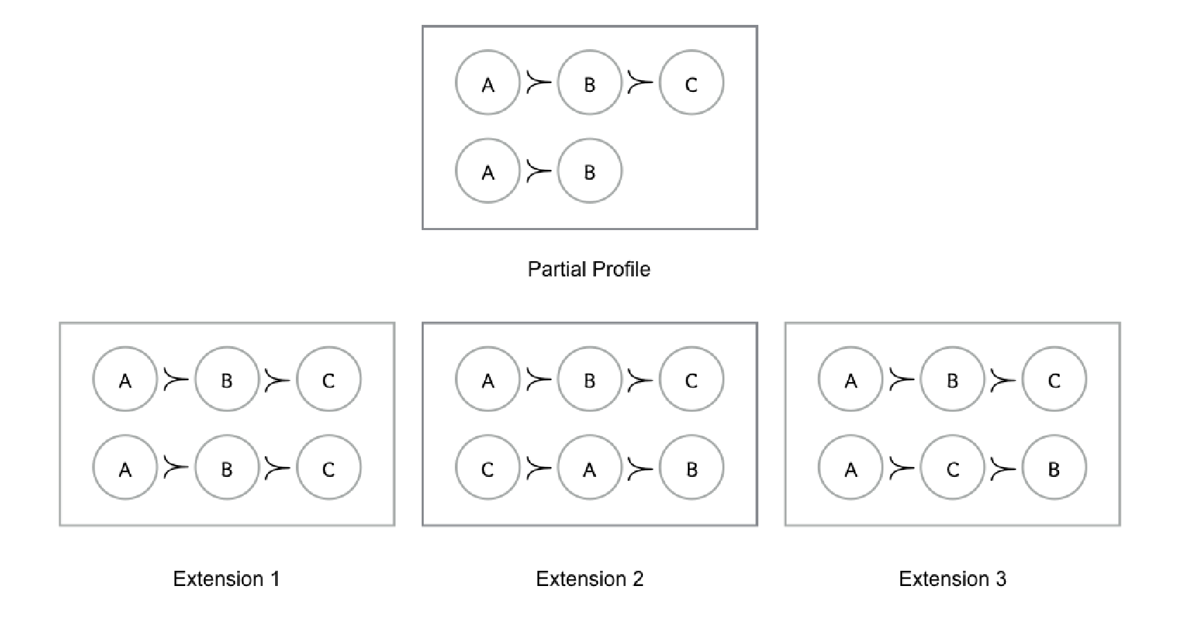
8.1.2 Related Work
A notion of manipulation under partial information has been considered by Conitzer et al. [68]. They focus on whether or not there exists a dominating manipulation and show that this problem is -hard for many common voting rules. Given some partial votes, a dominating manipulation is a non-truthful vote that the manipulator can cast which makes the winner at least as preferable (and sometimes more preferable) as the winner when the manipulator votes truthfully. The dominating manipulation problem and the Weak Manipulation, Opportunistic Manipulation, and Strong Manipulation problems do not seem to have any apparent complexity-theoretic connection. For example, the dominating manipulation problem is -hard for all the common voting rules except plurality and veto, whereas, the Strong Manipulation problem is easy for most of the cases (see Table 8.1). However, the results in [68] establish the fact that it is indeed possible to make manipulation intractable by restricting the amount of information the manipulators possess about the votes of the other voters. Elkind and Erdélyi [96] study manipulation under voting rule uncertainty. However, in our work, the voting rule is fixed and known to the manipulators.
Two closely related problems that have been extensively studied in the context of incomplete votes are Possible Winner and Necessary Winner [149]. In the Possible Winner problem, we are given a set of partial votes and a candidate , and the question is whether there exists an extension of where wins, while in the Necessary Winner problem, the question is whether is a winner in every extension of . Following the work in [149], a number of special cases and variants of the Possible Winner problem have been studied in the literature [52, 9, 38, 39, 128, 236, 77, 193, 25, 172]. The flavor of the Weak Manipulation problem is clearly similar to Possible Winner. However, we emphasize that there are subtle distinctions between the two problems. A more elaborate comparison is made in the next section.
8.1.3 Our Contribution
Our primary contribution in this work is to propose and study three natural and realistic generalizations of the computational problem of manipulation in the incomplete information setting. We summarize the complexity results in this work in Table 8.1. Our results provides the following interesting insights on the impact of lack of information on the computational difficulty of manipulation. We note that the number of undetermined pairs of candidates per vote are small constants in all our hardness results.
-
We observe that the computational problem of manipulation for the plurality and veto voting rules remains polynomial time solvable even with lack of information, irrespective of the notion of manipulation under consideration [Propositions 8.1, 8.15, 8.11 and 8.4]. We note that the plurality and veto voting rule also remain vulnerable under the notion of dominating manipulation [68].
-
The impact of absence of information on the computational complexity of manipulation is more dynamic for the -approval, -veto, Bucklin, Borda, and maximin voting rules. Only the Weak Manipulation and Opportunistic Manipulation problems are computationally intractable for the -approval [Theorems 8.1 and 8.5], -veto [Theorems 8.2 and 8.6], Bucklin [Theorems 8.3 and 8.10], Borda [8.3 and 8.7], and maximin [8.3 and 8.8] voting rules, whereas the Strong Manipulation problem remains computationally tractable [Theorems 8.11, 8.12, 8.13 and 8.14].
-
Table 8.1 shows an interesting behavior of the fallback voting rule. The Fallback voting rule is the only voting rule among the voting rules we study here for which the Weak Manipulation problem is NP-hard [Theorem 8.3] but both the Opportunistic Manipulation and Strong Manipulation problems are polynomial time solvable [Theorems 8.13 and 8.4]. This is because the Opportunistic Manipulation problem can be solved for the fallback voting rule by simply making manipulators vote for their desired candidate.
-
Our results show that absence of information makes all the three notions of manipulations intractable for the Copelandα voting rule for every rational for the Weak Manipulation problem [Observation 8.3] and for every for the Opportunistic Manipulation and Strong Manipulation problems [Theorems 8.4 and 8.9].
Our results (see Table 8.1) show that whether lack of information makes the manipulation problems harder, crucially depends on the notion of manipulation applicable to the situation under consideration. All the three notions of manipulations are, in our view, natural extension of manipulation to the incomplete information setting and tries to capture different behaviors of manipulators. For example, the Weak Manipulation problem may be applicable to an optimistic manipulator whereas for an pessimistic manipulator, the Strong Manipulation problem may make more sense.
| WM, | WM | OM, | OM | SM, | SM | |
| Plurality | ||||||
| Veto | P | P | ||||
| -Approval | ||||||
| -Veto | ||||||
| Bucklin | coNP-hard | |||||
| Fallback | NP-complete | P | P | |||
| Borda | ||||||
| maximin | P | |||||
| Copelandα | NP-complete | coNP-hard | coNP-hard | NP-hard | ||
8.1.4 Problem Definitions
We now formally define the three problems that we consider in this work, namely Weak Manipulation, Opportunistic Manipulation, and Strong Manipulation. Let be a fixed voting rule. We first introduce the Weak Manipulation problem.
Definition 8.1.
-Weak Manipulation
Given a set of partial votes over a set of candidates , a positive integer denoting the number of manipulators, and a candidate , do there exist votes such that there exists an extension of with ?
To define the Opportunistic Manipulation problem, we first introduce the notion of an -opportunistic voting profile, where is a voting rule and is any particular candidate.
Definition 8.2.
-Opportunistic Voting Profile
Let be the number of manipulators and a set of partial votes. An -voter profile is called an -opportunistic voting profile if for each extension of for which there exists an -vote profile with , we have .
In other words, an -vote profile is -opportunistic with respect to a partial profile if, when put together with the truthful votes of any extension, wins if the extension is viable to begin with. We are now ready to define the Opportunistic Manipulation problem.
Definition 8.3.
-Opportunistic Manipulation
Given a set of partial votes over a set of candidates , a positive integer denoting the number of manipulators, and a candidate , does there exist an -opportunistic -vote profile?
We finally define the Strong Manipulation problem.
Definition 8.4.
-Strong Manipulation
Given a set of partial votes over a set of candidates , a positive integer denoting the number of manipulators, and a candidate , do there exist votes such that for every extension of , we have ?
We use to denote instances of Weak Manipulation, Opportunistic Manipulation, and Strong Manipulation, where denotes a profile of partial votes, denotes the number of manipulators, and denotes the desired winner.
For the sake of completeness, we provide the definitions of the Coalitional Manipulation and Possible Winner problems below.
Definition 8.5.
-Coalitional Manipulation
Given a set of complete votes over a set of candidates , a positive integer denoting the number of manipulators, and a candidate , do there exist votes such that ?
Definition 8.6.
-Possible Winner
Given a set of partial votes and a candidate , does there exist an extension of the partial votes in to linear votes such that ?
8.1.5 Comparison with Possible Winner and Coalitional Manipulation Problems
For any fixed voting rule, the Weak Manipulation problem with manipulators reduces to the Possible Winner problem. This is achieved by simply using the same set as truthful votes and introducing empty votes. We summarize this in the observation below.
Observation 8.1.
The Weak Manipulation problem many-to-one reduces to the Possible Winner problem for every voting rule.
Proof.
Let be an instance of Weak Manipulation. Let be the set consisting of many copies of partial votes . Clearly the Weak Manipulation instance is equivalent to the Possible Winner instance . ∎
However, whether the Possible Winner problem reduces to the Weak Manipulation problem or not is not clear since in any Weak Manipulation problem instance, there must exist at least one manipulator and a Possible Winner instance may have no empty vote. From a technical point of view, the difference between the Weak Manipulation and Possible Winner problems may look marginal; however we believe that the Weak Manipulation problem is a very natural generalization of the Coalitional Manipulation problem in the partial information setting and thus worth studying. Similarly, it is easy to show, that the Coalitional Manipulation problem with manipulators reduces to Weak Manipulation, Opportunistic Manipulation, and Strong Manipulation problems with manipulators, since the former is a special case of the latter ones.
Observation 8.2.
The Coalitional Manipulation problem with manipulators many-to-one reduces to Weak Manipulation, Opportunistic Manipulation, and Strong Manipulation problems with manipulators for all voting rules and for all positive integers .
Proof.
Follows from the fact that every instance of the Coalitional Manipulation problem is also an equivalent instance of the Weak Manipulation, Opportunistic Manipulation, and Strong Manipulation problems. ∎
Finally, we note that the Coalitional Manipulation problem with manipulators can be reduced to the Weak Manipulation problem with just one manipulator, by introducing empty votes. These votes can be used to witness a good extension in the forward direction. In the reverse direction, given an extension where the manipulator is successful, the extension can be used as the manipulator’s votes. This argument leads to the following observation.
Observation 8.3.
The Coalitional Manipulation problem with manipulators many-to-one reduces to the Weak Manipulation problem with one manipulator for every voting rule and for every positive integer .
Proof.
Let be an instance of Coalitional Manipulation. Let be the set of consisting of many copies of partial vote . Clearly the Weak Manipulation instance is equivalent to the Coalitional Manipulation instance . ∎
This observation can be used to derive the hardness of Weak Manipulation even for one manipulator whenever the hardness for Coalitional Manipulation is known for any fixed number of manipulators (for instance, this is the case for the voting rules such as Borda, maximin and Copeland). However, determining the complexity of Weak Manipulation with one manipulator requires further work for voting rules where Coalitional Manipulation is polynomially solvable for any number of manipulators (such as -approval, Plurality, Bucklin, and so on).
8.2 Hardness Results for Weak Manipulation, Opportunistic Manipulation, and Strong Manipulation Problems
In this section, we present our hardness results. While some of our reductions are from the Possible Winner problem, the other reductions in this section are from the Exact Cover by 3-Sets problem, also referred to as X3C. This is a well-known -complete [125] problem, and is defined as follows.
Definition 8.7 (Exact Cover by 3-Sets (X3C)).
Given a set and a collection of subsets of with does there exist a with such that ?
We use to refer to the complement of X3C, which is to say that an instance of is a Yes instance if and only if it is a No instance of X3C. The rest of this section is organized according to the problems being addressed.
8.2.1 Weak Manipulation Problem
To begin with, recall that the Coalitional Manipulation problem is -complete for the Borda [75, 33], maximin [239], and Copelandα [113, 112, 114] voting rules for every rational , when we have two manipulators. Therefore, it follows from Observation 8.3 that the Weak Manipulation problem is -complete for the Borda, maximin, and Copelandα voting rules for every rational , even with one manipulator.
For the -approval and -veto voting rules, we reduce from the corresponding Possible Winner problems. While it is natural to start from the same voting profile, the main challenge is in undoing the advantage that the favorite candidate receives from the manipulator’s vote, in the reverse direction.
8.2.1.1 Result for the -Approval Voting Rule
We begin with proving that the Weak Manipulation problem is -complete for the -approval voting rule even with one manipulator and at most undetermined pairs per vote.
Theorem 8.1.
The Weak Manipulation problem is -complete for the -approval voting rule even with one manipulator for any constant , even when the number of undetermined pairs in each vote is no more than .
Proof.
For simplicity of presentation, we prove the theorem for -approval. We reduce from the Possible Winner problem for -approval which is -complete [236], even when the number of undetermined pairs in each vote is no more than . Let be the set of partial votes in a Possible Winner instance, and let be the set of candidates, where the goal is to check if there is an extension of that makes win. For developing the instance of Weak Manipulation, we need to “reverse” any advantage that the candidate obtains from the vote of the manipulator. Notice that the most that the manipulator can do is to increase the score of by one. Therefore, in our construction, we “artificially” increase the score of all the other candidates by one, so that despite of the manipulator’s vote, will win the new election if and only if it was a possible winner in the Possible Winner instance. To this end, we introduce many dummy candidates and the complete votes:
Further, we extend the given partial votes of the Possible Winner instance to force the dummy candidates to be preferred least over the rest - by defining, for every , the corresponding partial vote as follows.
This ensures that all the dummy candidates do not receive any score from the modified partial votes corresponding to the partial votes of the Possible Winner instance. Notice that since the number of undetermined pairs in is no more than , the number of undetermined pairs in is also no more than . Let denote this constructed Weak Manipulation instance. We claim that the two instances are equivalent.
In the forward direction, suppose is a possible winner with respect to , and let be an extension where wins. Then it is easy to see that the manipulator can make win in some extension by placing and in the first two positions of her vote (note that the partial score of is zero in ). Indeed, consider the extension of obtained by mimicking the extension on the “common” partial votes, . Notice that this is well-defined since and have exactly the same set of incomparable pairs. In this extension, the score of is strictly greater than the scores of all the other candidates, since the scores of all candidates in is exactly one more than their scores in , and all the dummy candidates have a score of at most one.
In the reverse direction, notice that the manipulator puts the candidates and in the top two positions without loss of generality. Now suppose the manipulator’s vote makes win the election for an extension of . Then consider the extension obtained by restricting to . Notice that the score of each candidate in in this extension is one less than their scores in . Therefore, the candidate wins this election as well, concluding the proof.
The above proof can be imitated for any other constant values of by reducing it from the Possible Winner problem for -approval and introducing dummy candidates. ∎
8.2.1.2 Result for the -Veto Voting Rule
Theorem 8.2.
The Weak Manipulation problem for the -veto voting rule is -complete even with one manipulator for any constant .
Proof.
We reduce from the Possible Winner problem for the -veto voting rule which is known to be -complete [19]. Let be the set of partial votes in a Possible Winner problem instance, and let be the set of candidates, where the goal is to check if there is an extension that makes win with respect to -veto. We assume without loss of generality that ’s position is fixed in all the partial votes (if not, then we fix the position of as high as possible in every vote).
We introduce many dummy candidates . The role of the first dummy candidates is to ensure that the manipulator is forced to place them at the “bottom ” positions of her vote, so that all the original candidates get the same score from the additional vote of the manipulator. The most natural way of achieving this is to ensure that the dummy candidates have the same score as in any extension (note that we know the score of since ’s position is fixed in all the partial votes). This would force the manipulator to place these candidates in the last positions. Indeed, doing anything else will cause these candidates to tie with , even when there is an extension of that makes win.
To this end, we begin by placing the dummy candidates in the top positions in all the partial votes. Formally, we modify every partial vote as follows:
At this point, we know the scores of and . Using Lemma 7.1, we add complete votes such that the final score of is the same with the score of every and the score of is strictly more than the score of . The relative score of every other candidate remains the same. This completes the description of the construction. We denote the augmented set of partial votes by .
We now argue the correctness. In the forward direction, if there is an extension of the votes that makes win, then we repeat this extension, and the vote of the manipulator puts the candidate at the position ; and all the other candidates in an arbitrary fashion. Formally, we let the manipulator’s vote be:
By construction wins the election in this particular setup. In the reverse direction, consider a vote of the manipulator and an extension of in which wins. Note that the manipulator’s vote necessarily places the candidates in the bottom positions — indeed, if not, then cannot win the election by construction. We extend a partial vote by mimicking the extension of the corresponding partial vote , that is, we simply project the extension of on the original set of candidates . Let denote this proposed extension of . We claim that wins the election given by . Indeed, suppose not. Let be a candidate whose score is at least the score of in the extension . Note that the scores of and in the extension are exactly the same as their scores in , except for a constant offset — importantly, their scores are offset by the same amount. This implies that the score of is at least the score of in as well, which is a contradiction. Hence, the two instances are equivalent. ∎
8.2.1.3 Result for the Bucklin Voting Rule
We next prove, by a reduction from X3C, that the Weak Manipulation problem for the Bucklin and simplified Bucklin voting rules is -complete even with one manipulator and at most undetermined pairs per vote.
Theorem 8.3.
The Weak Manipulation problem is -complete for Bucklin, simplified Bucklin, Fallback, and simplified Fallback voting rules, even when we have only one manipulator and the number of undetermined pairs in each vote is no more than .
Proof.
We reduce the X3C problem to Weak Manipulation for simplified Bucklin. Let be an instance of X3C, where each is a subset of of size three. We construct a Weak Manipulation instance based on as follows.
We first introduce the following partial votes in correspondence with the sets in the family as follows.
Notice that the number of undetermined pairs in every vote in is . We introduce the following additional complete votes :
-
copies of
-
copies of
-
copies of
The total number of voters, including the manipulator, is . Now we show equivalence of the two instances.
In the forward direction, suppose we have an exact set cover . Let the vote of the manipulator be . We consider the following extension of .
On the other hand, if , then we have:
We claim that is the unique simplified Bucklin winner in the profile . Notice that the simplified Bucklin score of is in this extension, since it appears in the top positions in the votes corresponding to the set cover, votes from the complete profile and one vote of the manipulator. For any other candidate , appears in the top positions once in and times in . Thus, does not get majority in top positions making its simplified Bucklin score at least . Hence, is the unique simplified Bucklin winner in the profile . Similarly, the candidate appears only times in the top positions. The same can be argued for the remaining candidates in and .
In the reverse direction, suppose the Weak Manipulation is a Yes instance. We may assume without loss of generality that the manipulator’s vote is , since the simplified Bucklin score of the candidates in is at least . Let be the extension of such that is the unique winner in the profile . As is ranked within top positions in votes in , for to win, must hold in at least votes in . In those votes, all the candidates in are also within top positions. Now if any candidate in is within top positions in more than once, then will not be the unique winner. Hence, the ’s corresponding to the votes where in form an exact set cover.
The reduction above also works for the Bucklin voting rule. Specifically, the argument for the forward direction is exactly the same as the simplified Bucklin above and the argument for the reverse direction is as follows. The candidate is ranked within top positions in votes in and is never placed within top positions in any vote in . Hence, for to win, must hold in at least votes in . In those votes, all the candidates in are also within top positions. Notice that never gets placed within top positions in any vote in . Now if any candidate is within top positions in more than once, then gets majority within top positions and thus cannot win.
The result for the Fallback and simplified Fallback voting rules follow from the corresponding results for the Bucklin and simplified Bucklin voting rules respectively since every Bucklin and simplified Bucklin election is also a Fallback and simplified Fallback election respectively. ∎
8.2.2 Strong Manipulation Problem
We know that the Coalitional Manipulation problem is -complete for the Borda, maximin, and Copelandα voting rules for every rational , when we have two manipulators. Thus, it follows from Observation 8.2 that Strong Manipulation is -hard for Borda, maximin, and Copelandα voting rules for every rational for at least two manipulators.
For the case of one manipulator, Strong Manipulation turns out to be polynomial-time solvable for most other voting rules. For Copelandα, however, we show that the problem is --hard for every for a single manipulator, even when the number of undetermined pairs in each vote is bounded by a constant. This is achieved by a careful reduction from .
We have following intractability result for the Strong Manipulation problem for the Copelandα rule with one manipulator and at most undetermined pairs per vote.
Theorem 8.4.
Strong Manipulation is --hard for Copelandα voting rule for every even when we have only one manipulator and the number of undetermined pairs in each vote is no more than .
Proof.
We reduce X3C to Strong Manipulation for Copelandα rule. Let is an X3C instance. We assume, without loss of generality, to be an even integer (if not, replicate any set from ). We construct a corresponding Weak Manipulation instance for Copelandα as follows.
Partial votes :
Notice that the number of undetermined pairs in every vote in is . Now we add a set of complete votes with even and using Lemma 7.2 to achieve the following margin of victories in pairwise elections.
-
-
-
-
-
-
for every not mentioned above
We have only one manipulator who tries to make winner. Notice that the number of votes in the Strong Manipulation instance including the manipulator’s vote is odd (since and are even integers). Therefore, is never zero for every in every extension of and manipulators vote and consequently the particular value of does not play any role in this reduction. Hence, we assume, without loss of generality, to be zero from here on and simply use the term Copeland instead of Copelandα.
Now we show that the X3C instance is a Yes instance if and only if the Strong Manipulation instance is a No instance (a Strong Manipulation instance is a No instance if there does not exist a vote of the manipulator which makes the unique winner in every extension of the partial votes). We can assume without loss of generality that manipulator puts at first position and at last position in her vote .
Assume that the X3C instance is a Yes instance. Suppose (by renaming) that forms an exact set cover. We claim that the following extension of makes both and Copeland co-winners.
Extension of :
We have summarize the pairwise margins between and and the rest of the candidates from the profile in Table 8.2. The candidates and are the co-winners with Copeland score .
For the other direction, notice that Copeland score of is at least since defeats and every candidate in in every extension of . Also notice that the Copeland score of can be at most since loses to and in every extension of . Hence the only way cannot be the unique winner is that defeats all candidates in and defeats .
This requires in at least extensions of . We claim that the sets in the remaining of the extensions where forms an exact set cover for . Indeed, otherwise some candidate is not covered. Then, notice that in all votes, making . ∎
8.2.3 Opportunistic Manipulation Problem
All our reductions for the --hardness for Opportunistic Manipulation start from . We note that all our hardness results hold even when there is only one manipulator. Our overall approach is the following. We engineer a set of partial votes in such a way that the manipulator is forced to vote in a limited number of ways to have any hope of making her favorite candidate win. For each such vote, we demonstrate a viable extension where the vote fails to make the candidate a winner, leading to a No instance of Opportunistic Manipulation. These extensions rely on the existence of an exact cover. On the other hand, we show that if there is no exact set cover, then there is no viable extension, thereby leading to an instance that is vacuously a Yes instance of Opportunistic Manipulation.
8.2.3.1 Result for the -Approval Voting Rule
Our first result on Opportunistic Manipulation shows that the Opportunistic Manipulation problem is --hard for the -approval voting rule for constant even when the number of manipulators is one and the number of undetermined pairs in each vote is no more than .
Theorem 8.5.
The Opportunistic Manipulation problem is --hard for the -approval voting rule for constant even when the number of manipulators is one and the number of undetermined pairs in each vote is no more than .
Proof.
We reduce to Opportunistic Manipulation for -approval rule. Let is an instance. We construct a corresponding Opportunistic Manipulation instance for -approval voting rule as follows. We begin by introducing a candidate for every element of the universe, along with dummy candidates (denoted by ), and special candidates . Formally, we have:
Now, for every set in the universe, we define the following total order on the candidate set, which we denote by :
Using , we define the partial vote as follows:
We denote the set of partial votes by and by . We remark that the number of undetermined pairs in each partial vote is .
We now invoke Lemma 1 from [88], which allows to achieve any pre-defined scores on the candidates using only polynomially many additional votes. Using this, we add a set of complete votes with to ensure the following scores, where we denote the -approval score of a candidate from a set of votes by : .
Our reduced instance is . The reasoning for this score configuration will be apparent as we argue the equivalence. We first argue that if we had a Yes instance of (in other words, there is no exact cover), then we have a Yes instance of Opportunistic Manipulation. It turns out that this will follow from the fact that there are no viable extensions, because, as we will show next, a viable extension implies the existence of an exact set cover.
To this end, first observe that the partial votes are constructed in such a way that gets no additional score from any extension. Assuming that the manipulator approves (without loss of generality), the final score of in any extension is going to be . Now, in any viable extension, every candidate has to be “pushed out” of the top positions at least once. Observe that whenever this happens, is forced into the top positions. Since is behind the score of by only votes, ’s can be pushed out of place in only votes. For every to lose one point, these votes must correspond to an exact cover. Therefore, if there is no exact cover, then there is no viable extension, showing one direction of the reduction.
On the other hand, suppose we have a No instance of – that is, there is an exact cover. We will now use the exact cover to come up with two viable extensions, both of which require the manipulator to vote in different ways to make win. Therefore, there is no single manipulative vote that accounts for both extensions, leading us to a No instance of Opportunistic Manipulation.
First, consider this completion of the partial votes:
Notice that in this completion, once accounted for along with the votes in , the score of is tied with the scores of all ’s, and , while the score of is one less than the score of . Therefore, the only candidates that the manipulator can afford to approve are , the candidates and . However, consider the extension that is identical to the above except with the first vote changed to:
Here, on the other hand, the only way for to be an unique winner is if the manipulator approves and . Therefore, it is clear that there is no way for the manipulator to provide a consolidated vote for both these profiles. Therefore, we have a No instance of Opportunistic Manipulation. ∎
8.2.3.2 Result for the -Veto Voting Rule
We next move on to the -veto voting rule and show that the Opportunistic Manipulation problem for the -veto is --hard for every constant even when the number of manipulators is one and the number of undetermined pairs in each vote is no more than .
Theorem 8.6.
The Opportunistic Manipulation problem is --hard for the -veto voting rule for every constant even when the number of manipulators is one and the number of undetermined pairs in each vote is no more than .
Proof.
We reduce X3C to Opportunistic Manipulation for -veto rule. Let is an X3C instance. We construct a corresponding Opportunistic Manipulation instance for -veto voting rule as follows.
For every , we define as follows:
Using , we define partial vote for every . We denote the set of partial votes by and by . We note that the number of undetermined pairs in each partial vote is . Using Lemma 7.1, we add a set of complete votes with to ensure the following. We denote the -veto score of a candidate from a set of votes by .
We have only one manipulator who tries to make winner. Now we show that the X3C instance is a Yes instance if and only if the Opportunistic Manipulation instance is a No instance.
In the forward direction, let us now assume that the X3C instance is a Yes instance. Suppose (by renaming) that forms an exact set cover. Let us assume that the manipulator’s vote disapproves every candidate in since otherwise can never win uniquely. We now show that if does not disapprove then, is not a -optimal vote. Suppose does not disapprove . Then we consider the following extension of .
We have the following scores . Hence, both and win for the votes . However, the vote which disapproves makes a unique winner for the votes . Hence, is not a -optimal vote. Similarly, we can show that if the manipulator’s vote does not disapprove then, the vote is not -optimal. Hence, there does not exist any -optimal vote and the Opportunistic Manipulation instance is a No instance.
In the reverse direction, we show that if the X3C instance is a No instance, then there does not exist a vote of the manipulator and an extension of such that is the unique winner for the votes thereby proving that the Opportunistic Manipulation instance is vacuously Yes (and thus every vote is -optimal). Notice that, there must be at least votes in where the corresponding gets pushed in bottom positions since . However, in each vote in , is placed within top many position and thus we have is exactly since . Now notice that there must be at least one candidate which is not covered by the sets s corresponding to the votes because the X3C instance is a No instance. Hence, cannot win the election uniquely irrespective of the manipulator’s vote. Thus every vote is -optimal and the Opportunistic Manipulation instance is a Yes instance. ∎
8.2.3.3 Result for the Borda Voting Rule
We show next similar intractability result for the Borda voting rule too with only at most undetermined pairs per vote.
Theorem 8.7.
The Opportunistic Manipulation problem is --hard for the Borda voting rule even when the number of manipulators is one and the number of undetermined pairs in every vote is no more than .
Proof.
We reduce X3C to Opportunistic Manipulation for the Borda rule. Let is an X3C instance. Without loss of generality we assume that is not divisible by (if not, then we add three new elements to and a set to ). We construct a corresponding Opportunistic Manipulation instance for the Borda voting rule as follows.
For every , we define as follows:
Using , we define partial vote for every . We denote the set of partial votes by and by . We note that the number of undetermined pairs in each partial vote is . Using Lemma 7.1, we add a set of complete votes with to ensure the following. We denote the Borda score of a candidate from a set of votes by .
We have only one manipulator who tries to make winner. Now we show that the X3C instance is a Yes instance if and only if the Opportunistic Manipulation instance is a No instance. Notice that we can assume without loss of generality that the manipulator places at the first position, at the second position, the candidate at position for every , and at the last position, since otherwise can never win uniquely irrespective of the extension of (that it, the manipulator’s vote looks like ).
In the forward direction, let us now assume that the X3C instance is a Yes instance. Suppose (by renaming) that forms an exact set cover. Let the manipulator’s vote be . We now argue that is not a -optimal vote. The other case where the manipulator’s vote be can be argued similarly. We consider the following extension of .
We have the following Borda scores . Hence, does not win uniquely for the votes . However, is the unique winner for the votes . Hence, there does not exist any -optimal vote and the Opportunistic Manipulation instance is a No instance.
In the reverse direction, we show that if the X3C instance is a No instance, then there does not exist a vote of the manipulator and an extension of such that is the unique winner for the votes thereby proving that the Opportunistic Manipulation instance is vacuously Yes (and thus every vote is -optimal). Notice that the score of must decrease by at least for to win uniquely. However, in every vote where the score of decreases by at least one in any extension of , at least one of or must be placed at top position of the vote . However, the candidates and can be placed at top positions of the votes in at most many times while ensuring does not lose the election. Also, even after manipulator places the candidate at position for every , for to win uniquely, the score of every must decrease by at least one. Hence, altogether, there will be exactly votes (denoted by the set ) in any extension of where is placed at the second position. However, since the X3C instance is a No instance, the s corresponding to the votes in does not form a set cover. Let be an element not covered by the s corresponding to the votes in . Notice that the score of does not decrease in the extension and thus does not win uniquely irrespective of the manipulator’s vote. Thus every vote is -optimal and thus the Opportunistic Manipulation instance is a Yes instance. Thus every vote is -optimal and the Opportunistic Manipulation instance is a Yes instance. ∎
8.2.3.4 Result for the Maximin Voting Rule
For the maximin voting rule, we show intractability of Opportunistic Manipulation with one manipulator even when the number of undetermined pairs in every vote is at most .
Theorem 8.8.
The Opportunistic Manipulation problem is --hard for the maximin voting rule even when the number of manipulators is one and the number of undetermined pairs in every vote is no more than .
Proof.
We reduce X3C to Opportunistic Manipulation for the maximin rule. Let is an X3C instance. We construct a corresponding Opportunistic Manipulation instance for the maximin voting rule as follows.
For every , we define as follows:
Using , we define partial vote for every . We denote the set of partial votes by and by . We note that the number of undetermined pairs in each partial vote is . We define another partial vote as follows.
Using Lemma 7.2, we add a set of complete votes with to ensure the following pairwise margins (notice that the pairwise margins among and does not include the partial vote ).
-
-
-
-
-
-
for every not defined above.
We have only one manipulator who tries to make winner. Now we show that the X3C instance is a Yes instance if and only if the Opportunistic Manipulation instance is a No instance. Notice that we can assume without loss of generality that the manipulator’s vote prefers to every other candidate, to , to , and to for every .
In the forward direction, let us now assume that the X3C instance is a Yes instance. Suppose (by renaming) that forms an exact set cover. Notice that the manipulator’s vote must prefer either to or to or to . We show that if the manipulator’s vote prefers to , then is not a -optimal vote. The other two cases are symmetrical. Consider the following extension of and of .
From the votes in , the maximin score of is , of are , of are at most than , and of is . Hence, is not the unique maximn winner. However, the manipulator’s vote makes the unique maximin winner. Hence, is not a -optimal vote.
For the reverse direction, we show that if the X3C instance is a No instance, then there does not exist a vote of the manipulator and an extension of such that is the unique winner for the votes thereby proving that the Opportunistic Manipulation instance is vacuously Yes (and thus every vote is -optimal). Consider any extension of . Notice that, for to win uniquely, must be at least of the votes in ; call these set of votes . However, in every vote in and can be in at most votes in for to win uniquely. Hence, we have . Also for to win, each must be at least one vote of and is possible only in the votes in . However, the sets s corresponding to the votes in does not form a set cover since the X3C instance is a No instance. Hence, there must exist a for which in every vote in and thus cannot win uniquely irrespective of the vote of the manipulator. Thus every vote is -optimal and the Opportunistic Manipulation instance is a Yes instance. ∎
8.2.3.5 Result for the Copelandα Voting Rule
Our next result proves that the Opportunistic Manipulation problem is --hard for the Copelandα voting rule too for every even with one manipulator and at most undetermined pairs per vote.
Theorem 8.9.
The Opportunistic Manipulation problem is --hard for the Copelandα voting rule for every even when the number of manipulators is one and the number of undetermined pairs in each vote is no more than .
Proof.
We reduce X3C to Opportunistic Manipulation for the Copelandα voting rule. Let is an X3C instance. We construct a corresponding Opportunistic Manipulation instance for the Copelandα voting rule as follows.
For every , we define as follows:
Using , we define partial vote for every . We denote the set of partial votes by and by . We note that the number of undetermined pairs in each partial vote is . We define another partial vote as follows.
Using Lemma 7.2, we add a set of complete votes with to ensure the following pairwise margins (notice that the pairwise margins among and does not include the partial vote ).
-
-
-
-
for at least many
-
-
for every not defined above.
We have only one manipulator who tries to make winner. Now we show that the X3C instance is a Yes instance if and only if the Opportunistic Manipulation instance is a No instance. Since the number of voters is odd, does not play any role in the reduction and thus from here on we simply omit . Notice that we can assume without loss of generality that the manipulator’s vote prefers to every other candidate and to .
In the forward direction, let us now assume that the X3C instance is a Yes instance. Suppose (by renaming) that forms an exact set cover. Suppose the manipulator’s vote order and as . We will show that is not a -optimal vote. Symmetrically, we can show that the manipulator’s vote ordering and in any other order is not -optimal. Consider the following extension of and of .
From the votes in , the Copeland score of is (defeating ), of is (defeating ), of is at most (defeating and at most many ), of is (defeating ), of is (defeating and ), of is (defeating ). of is (defeating ) for every , of is (defeating ), is (defeating ), is (defeating ). Hence, co-wins with with Copeland score . However, the manipulator’s vote makes win uniquely. Hence, is not a -optimal vote and thus the Opportunistic Manipulation instance is a No instance.
For the reverse direction, we show that if the X3C instance is a No instance, then there does not exist a vote of the manipulator and an extension of such that is the unique winner for the votes thereby proving that the Opportunistic Manipulation instance is vacuously Yes (and thus every vote is -optimal). Consider any extension of . Notice that, for to win uniquely, must defeat each and thus is preferred over in at least one vote in ; we call these votes . However, in every vote in , is preferred over and thus because must defeat for to win uniquely. Since the X3C instance is a No instance, there must be a candidate which is not covered by the sets corresponding to the votes in and thus is preferred over in every vote in . Hence, cannot win uniquely irrespective of the vote of the manipulator. Thus every vote is -optimal and the Opportunistic Manipulation instance is a Yes instance. ∎
8.2.3.6 Result for the Bucklin Voting Rule
For the Bucklin and simplified Bucklin voting rules, we show intractability of the Opportunistic Manipulation problem with at most undetermined pairs per vote and only one manipulator.
Theorem 8.10.
The Opportunistic Manipulation problem is --hard for the Bucklin and simplified Bucklin voting rules even when the number of manipulators is one and the number of undetermined pairs in each vote is no more than .
Proof.
We reduce X3C to Opportunistic Manipulation for the Bucklin and simplified Bucklin voting rules. Let is an X3C instance. We assume without loss of generality that is not divisible by (if not, we introduce three elements in and a set containing them in ) and is an even integer (if not, we duplicate any set in ). We construct a corresponding Opportunistic Manipulation instance for the Bucklin and simplified Bucklin voting rules as follows.
For every , we define as follows:
Using , we define partial vote for every . We denote the set of partial votes by and by . We note that the number of undetermined pairs in each partial vote is . We introduce the following additional complete votes :
-
copies of
-
copies of
-
copies of
-
copies of
-
copies of
-
copies of
-
One
We have only one manipulator who tries to make winner. Now we show that the X3C instance is a Yes instance if and only if the Opportunistic Manipulation instance is a No instance. The total number of voters in the Opportunistic Manipulation instance is . We notice that within top positions of the votes in , appears times, and appear times, appears times, appears times, every candidate in appears times, every candidate in appears times. Also every candidate in appears times within top positions of the votes in . Hence, for both Bucklin and simplified Bucklin voting rules, we can assume without loss of generality that the manipulator puts , every candidate in , , , and exactly one of and .
In the forward direction, let us now assume that the X3C instance is a Yes instance. Suppose (by renaming) that forms an exact set cover. Suppose the manipulator’s vote puts , every candidate in , , , and within top positions. We will show that is not -optimal. The other case where the manipulator’s vote puts , every candidate in , , , and within top positions is symmetrical. Consider the following extension of :
For both Bucklin and simplified Bucklin voting rules, co-wins with for the votes in . However, wins uniquely for the votes in . Hence, is not a -optimal vote and thus the Opportunistic Manipulation instance is a No instance.
For the reverse direction, we show that if the X3C instance is a No instance, then there does not exist a vote of the manipulator and an extension of such that is the unique winner for the votes thereby proving that the Opportunistic Manipulation instance is vacuously Yes (and thus every vote is -optimal). Consider any extension of . Notice that, for to win uniquely, every candidate must be pushed out of top positions in at least one vote in ; we call these set of votes . Notice that, . However, in every vote in , at least one of and appears within top many positions. Since, the manipulator has to put at least one of and within its top positions and and appear times in the votes in , we must have and thus , for to win uniquely. However, there exists a candidate not covered by the s corresponding to the votes in . Notice that gets majority within top positions of the votes and can never get majority within top positions of the votes. Hence, cannot win uniquely irrespective of the vote of the manipulator. Thus every vote is -optimal and the Opportunistic Manipulation instance is a Yes instance. ∎
8.3 Polynomial Time Algorithms for Weak Manipulation, Strong Manipulation, and Opportunistic Manipulation Problems
We now turn to the polynomial time cases depicted in Table 8.1. This section is organized in three parts, one for each problem considered.
8.3.1 Weak Manipulation Problem
Since the Possible Winner problem is in for the plurality and the veto voting rules [19], it follows from Observation 8.1 that the Weak Manipulation problem is in for the plurality and veto voting rules for any number of manipulators.
Proposition 8.1.
The Weak Manipulation problem is in for the plurality and veto voting rules for any number of manipulators.
Proof.
The Possible Winner problem is in for the plurality and the veto voting rules [19]. Hence, the result follows from Observation 8.1. ∎
8.3.2 Strong Manipulation Problem
We now discuss our algorithms for the Strong Manipulation problem. The common flavor in all our algorithms is the following: we try to devise an extension that is as adversarial as possible for the favorite candidate , and if we can make win in such an extension, then roughly speaking, such a strategy should work for other extensions as well (where the situation only improves for ). However, it is challenging to come up with an extension that is globally dominant over all the others in the sense that we just described. So what we do instead is we consider every potential nemesis who might win instead of , and we build profiles that are “as good as possible” for and “as bad as possible” for . Each such profile leads us to constraints on how much the manipulators can afford to favor (in terms of which positions among the manipulative votes are safe for ). We then typically show that we can determine whether there exists a set of votes that respects these constraints, either by using a greedy strategy or by an appropriate reduction to a flow problem. We note that the overall spirit here is similar to the approaches commonly used for solving the Necessary Winner problem, but as we will see, there are non-trivial differences in the details. We begin with the -approval and -veto voting rules.
Theorem 8.11.
The Strong Manipulation problem is in for the -approval and -veto voting rules, for any and any number of manipulators.
Proof.
For the time being, we just concentrate on non-manipulators’ votes. For each candidate , calculate the maximum possible value of from non-manipulators’ votes, where is the score that candidate receives from the votes of the non-manipulators. This can be done by checking all possible pairs of positions for and in each vote and choosing the one which maximizes from that vote. We now fix the position of at the top position for the manipulators’ votes and we check if it is possible to place other candidates in the manipulators’ votes such that the final value of is negative which can be solved easily by reducing it to the max flow problem which is polynomial time solvable. ∎
We now prove that the Strong Manipulation problem for scoring rules is in for one manipulator.
Theorem 8.12.
The Strong Manipulation problem is in for any scoring rule when we have only one manipulator.
Proof.
For each candidate , calculate using same technique described in the proof of Theorem 8.11. We now put at the top position of the manipulator’s vote. For each candidate , can be placed at positions in the manipulator’s vote which makes negative. Using this, construct a bipartite graph with on left and on right and there is an edge between and iff the candidate can be placed at in the manipulator’s vote according to the above criteria. Now solve the problem by finding existence of perfect matching in this graph. ∎
Our next result proves that the Strong Manipulation problem for the Bucklin, simplified Bucklin, fallback, and simplified fallback voting rules are in .
Theorem 8.13.
The Strong Manipulation problem is in for the Bucklin, simplified Bucklin, fallback, and simplified fallback voting rules, for any number of manipulators.
Proof.
Let be an instance of Strong Manipulation for simplified Bucklin, and let denote the total number of candidates in this instance. Recall that the manipulators have to cast their votes so as to ensure that the candidate wins in every possible extension of . We use to denote the set of manipulating votes that we will construct. To begin with, without loss of generality, the manipulators place in the top position of all their votes. We now have to organize the positioning of the remaining candidates across the votes of the manipulators to ensure that is a necessary winner of the profile .
To this end, we would like to develop a system of constraints indicating the overall number of times that we are free to place a candidate among the top positions in the profile . In particular, let us fix and . Let be the maximum number of votes of in which can appear in the top positions. Our first step is to compute necessary conditions for .
We use to denote a set of complete votes that we will construct based on the given partial votes. Intuitively, these votes will represent the “worst” possible extensions from the point of view of when pitted against . These votes are engineered to ensure that the manipulators can make win the elections for all and , if, and only if, they can strongly manipulate in favor of . More formally, there exists a voting profile of the manipulators so that wins the election , for all and if and only if wins in every extension of the profile .
We now describe the profile . The construction is based on the following case analysis, where our goal is to ensure that, to the extent possible, we position out of the top positions, and incorporate among the top positions.
-
Let be such that either and are incomparable or . We add the complete vote to , where is obtained from by placing at the highest possible position and at the lowest possible position, and extending the remaining vote arbitrarily.
-
Let be such that , but there are at least candidates that are preferred over in . We add the complete vote to , where is obtained from by placing at the lowest possible position, and extending the remaining vote arbitrarily.
-
Let be such that is forced to be within the top positions, then we add the complete vote to , where is obtained from by first placing at the highest possible position followed by placing at the lowest possible position, and extending the remaining vote arbitrarily.
-
In the remaining votes, notice that whenever is in the top positions, is also in the top positions. Let denote this set of votes, and let be the number of votes in .
We now consider two cases. Let be the number of times is placed in the top positions in the profile , and let be the number of times is placed in the top positions in the profile . Let us now formulate the requirement that in , the candidate does not have a majority in the top positions and does have a majority in the top positions. Note that if this requirement holds for any and , then strong manipulation is not possible. Therefore, to strongly manipulate in favor of , we must ensure that for every choice of and , we are able to negate the conditions that we derive.
The first condition from above simply translates to . The second condition amounts to requiring first, that there are at least votes where appears in the top positions, that is, . Further, note that the gap between and majority will be filled by using votes from to “push” forward. However, these votes contribute equally to and being in the top and positions, respectively. Therefore, the difference between and must be less than the difference between and . Summarizing, the following conditions, which we collectively denote by , are sufficient to defeat in some extension: .
From the manipulator’s point of view, the above provides a set of constraints to be satisfied as they place the remaining candidates across their votes. Whenever , the manipulators place any of the other candidates among the top positions freely, because already has majority. On the other hand, if , then the manipulators must respect at least one of the following constraints: and .
Extending the votes of the manipulator while respecting these constraints (or concluding that this is impossible to do) can be achieved by a natural greedy strategy — construct the manipulators’ votes by moving positionally from left to right. For each position, consider each manipulator and populate her vote for that position with any available candidate. We output the profile if the process terminates by completing all the votes, otherwise, we say No.
We now argue the proof of correctness. Suppose the algorithm returns No. This implies that there exists a choice of and such that for any voting profile of the manipulators, the conditions in are satisfied. (Indeed, if there exists a voting profile that violated at least one of these conditions, then the greedy algorithm would have discovered it.) Therefore, no matter how the manipulators cast their vote, there exists an extension where is defeated. In particular, for the votes in , this extension is given by . Further, we choose votes among the votes in and extend them by placing in the top positions (and extending the rest of the profile arbitrary). We extend the remaining votes in by positioning outside the top positions. Clearly, in this extension, fails to achieve majority in the top positions while does achieve majority in the top positions.
On the other hand, if the algorithm returns Yes, then consider the voting profile of the manipulators. We claim that wins in every extension of . Suppose, to the contrary, that there exists an extension and a candidate such that the simplified Bucklin score of is no more than the simplified Bucklin score of in . In this extension, therefore, there exists for which attains majority in the top positions and fails to attain majority in the top positions. However, note that this is already impossible in any extension of the profile , because of the design of the constraints. By construction, the number of votes in which appears in the top positions in is only greater than the number of times appears in the top positions in any extension of (and similarly for ). This leads us to the desired contradiction.
For the Bucklin voting rule, we do the following modifications to the algorithm. If for some and , then we make . The proof of correctness for the Bucklin voting rule is similar to the proof of correctness for the simplified Bucklin voting rule above.
For Fallback and simplified Fallback voting rules, we consider the number of candidates each voter approves while computing . We output Yes if and only if for every and every , since we can assume, without loss of generality, that the manipulator approves the candidate only. Again the proof of correctness is along similar lines to the proof of correctness for the simplified Bucklin voting rule. ∎
We next show that the Strong Manipulation problem for the maximin voting rule is polynomial-time solvable when we have only one manipulator.
Theorem 8.14.
The Strong Manipulation problem for the maximin voting rules are in , when we have only one manipulator.
Proof.
For the time being, just concentrate on non-manipulators’ votes. Using the algorithm for NW for maximin in [236], we compute for all pairs , and for all . This can be computed in polynomial time. Now we place at the top position in the manipulator’s vote and increase all by one. Now we place a candidate at the second position if for all , for all , where of the candidate has already been assigned some position in the manipulator’s vote, and else. The correctness argument is in the similar lines of the classical greedy manipulation algorithm of [41]. ∎
8.3.3 Opportunistic Manipulation Problem
For the plurality, fallback, and simplified fallback voting rules, it turns out that the voting profile where all the manipulators approve only is a -opportunistic voting profile, and therefore it is easy to devise a manipulative vote.
Observation 8.4.
The Opportunistic Manipulation problem is in for the plurality and fallback voting rules for a any number of manipulators.
For the veto voting rule, however, a more intricate argument is needed, that requires building a system of constraints and a reduction to a suitable instance of the maximum flow problem in a network, to show polynomial time tractability of Opportunistic Manipulation.
Theorem 8.15.
The Opportunistic Manipulation problem is in for the veto voting rule for a constant number of manipulators.
Proof.
Let be an input instance of Opportunistic Manipulation. We may assume without loss of generality that the manipulators approve . We view the voting profile of the manipulators as a tuple with , where the many manipulators disapprove . We denote the set of such tuples as and we have which is polynomial in since is a constant. A tuple is not -optimal if there exists another tuple and an extension of with the following properties. We denote the veto score of a candidate from by . For every candidate , we define two quantities and as follows.
-
for every with and we define
-
for every with and we define
-
for every with and we define
We guess the value of . Given a value of , we check the above two conditions by reducing this to a max flow problem instance as follows. We have a source vertex and a sink . We have a vertex for every (call this set of vertices ) and a vertex for every vote (call this set of vertices ). We add an edge from to each in of capacity one. We add an edge of capacity one from a vertex to a vertex if the candidate corresponding to the vertex can be placed at the last position in an extension of the partial vote corresponding to the vertex . We add an edge from a vertex to of capacity , where is the voter corresponding to the vertex . We also set the demand of every vertex (that is the total amount of flow coming into vertex must be at least ), where is the voter corresponding to the vertex . Clearly, the above three conditions are met if and only if there is a feasible amount of flow in the above flow graph. Since can have only possible values (from to ) and , we can iterate over all possible pairs of tuples in and all possible values of and find a -optimal voting profile if there exists a one. ∎
8.4 Conclusion
We revisited many settings where the complexity barrier for manipulation was non-existent, and studied the problem under an incomplete information setting. Our results present a fresh perspective on the use of computational complexity as a barrier to manipulation, particularly in cases that were thought to be dead-ends (because the traditional manipulation problem was polynomially solvable). To resurrect the argument of computational hardness, we have to relax the model of complete information, but we propose that the incomplete information setting is more realistic, and many of our hardness results work even with very limited amount of incompleteness in information.
In the next chapter, we will see how possible instances of manipulation can be detected for various voting rules.
Chapter 9 Manipulation Detection
†† A preliminary version of the work in this chapter was published as [84]: Palash Dey, Neeldhara Misra, and Y. Narahari. Detecting possible manipulators in elections. In Proc. 2015 International Conference on Autonomous Agents and Multiagent Systems, AAMAS 2015, Istanbul, Turkey, May 4-8, 2015, pages 1441-1450, 2015.Manipulation is a problem of fundamental importance in voting theory in which the voters exercise their votes strategically instead of voting honestly to make an alternative that is more preferred to her, win the election. The classical Gibbard-Satterthwaite theorem shows that there is no strategy-proof voting rule that simultaneously satisfies certain combination of desirable properties. Researchers have attempted to get around the impossibility result in several ways such as domain restriction and computational hardness of manipulation. However, these approaches are known to have fundamental limitations. Since prevention of manipulation seems to be elusive even after substantial research effort, an interesting research direction therefore is detection of manipulation. Motivated by this, we initiate the study of detecting possible instances of manipulation in elections.
We formulate two pertinent computational problems in the context of manipulation detection - Coalitional Possible Manipulators (CPM) and Coalitional Possible Manipulators given Winner (CPMW), where a suspect group of voters is provided as input and we have to find whether they can be a potential coalition of manipulators. In the absence of any suspect group, we formulate two more computational problems namely Coalitional Possible Manipulators Search (CPMS) and Coalitional Possible Manipulators Search given Winner (CPMSW). We provide polynomial time algorithms for these problems, for several popular voting rules. For a few other voting rules, we show that these problems are -complete. We observe that detecting possible instances of manipulation may be easy even when the actual manipulation problem is computationally intractable, as seen for example, in the case of the Borda voting rule.
9.1 Introduction
A basic problem with voting rules is that the voters may vote strategically instead of voting honestly, leading to the selection of a candidate which is not the actual winner. We call a candidate actual winner if it wins the election when every voter votes truthfully. This phenomenon of strategic voting is called manipulation in the context of voting. The Gibbard-Satterthwaite (G-S) theorem [124, 213] proves that manipulation is unavoidable for any unanimous and non-dictatorial voting rule if we have at least three candidates. A voting rule is called unanimous if whenever any candidate is most preferred by all the voters, such a candidate is the winner. A voting rule is called non-dictatorial if there does not exist any voter whose most preferred candidate is always the winner irrespective of the votes of other voters. The problem of manipulation is particularly relevant for multiagent systems since agents have computational power to determine strategic votes. There have been several attempts to bypass the impossibility result of the G-S theorem.
Economists have proposed domain restriction as a way out of the impossibility implications of the G-S theorem. The G-S theorem assumes all possible preference profiles as the domain of voting rules. In a restricted domain, it has been shown that we can have voting rules that are not vulnerable to manipulation. A prominent restricted domain is the domain of single peaked preferences, in which the median voting rule provides a satisfactory solution [168]. To know more about other domain restrictions, we refer to [168, 123]. This approach of restricting the domain, however, suffers from the requirement that the social planner needs to know the domain of preference profiles of the voters, which is often impractical.
9.1.1 Related Work
Researchers in computational social choice theory have proposed invoking computational intractability of manipulation as a possible work around for the G-S theorem. Bartholdi et al. [34, 41] first proposed the idea of using computational hardness as a barrier against manipulation. Bartholdi et al. defined and studied the computational problem called manipulation where a set of manipulators have to compute their votes that make their preferred candidate win the election. The manipulators know the votes of the truthful voters and the voting rule that will be used to compute the winner. Following this, a large body of research [194, 75, 239, 237, 65, 197, 100, 111, 192, 126, 196, 110, 246, 90, 120, 96] shows that the manipulation problem is -complete for many voting rules. However, Procaccia et al. [203, 204] showed average case easiness of manipulation assuming junta distribution over the voting profiles. Friedgut et al. [115] showed that any neutral voting rule which is sufficiently far from being dictatorial is manipulable with non-negligible probability at any uniformly random preference profile by a uniformly random preference. The above result holds for elections with three candidates only. A voting rule is called neutral if the names of the candidates are immaterial. Isaksson et al. [143] generalize the above result to any number of candidates which has been further generalized to all voting rules which may not be neutral by Mossel and Racz in [184]. Walsh [229] empirically shows ease of manipulating an STV (single transferable vote) election – one of the very few voting rules where manipulation, even by one voter, is -complete [34]. In addition to the results mentioned above, there exist many other results in the literature that emphasize the weakness of considering computational complexity as a barrier against manipulation [64, 235, 234, 119, 230]. Hence, the barrier of computational hardness is ineffective against manipulation in many settings.
9.1.2 Motivation
In a situation where multiple attempts for prevention of manipulation fail to provide a fully satisfactory solution, detection of manipulation is a natural next step of research. There have been scenarios where establishing the occurrence of manipulation is straightforward, by observation or hindsight. For example, in sport, there have been occasions where the very structure of the rules of the game have encouraged teams to deliberately lose their matches. Observing such occurrences in, for example, football (the 1982 FIFA World Cup football match played between West Germany and Austria) and badminton (the quarter-final match between South Korea and China in the London 2012 Olympics), the relevant authorities have subsequently either changed the rules of the game (as with football) or disqualified the teams in question (as with the badminton example). The importance of detecting manipulation lies in the potential for implementing corrective measures in the future. For reasons that will be evident soon, it is not easy to formally define the notion of manipulation detection. Assume that we have the votes from an election that has already happened. A voter is potentially a manipulator if there exists a preference , different from the voter’s reported preference, which is such that the voter had an “incentive to deviate” from the . Specifically, suppose the candidate who wins with respect to this voter’s reported preference is preferred (in ) over the candidate who wins with respect to . In such a situation, could potentially be the voter’s truthful preference, and the voter could be refraining from being truthful because an untruthful vote leads to a more favorable outcome with respect to . Note that we do not (and indeed, cannot) conclusively suggest that a particular voter has manipulated an election. This is because the said voter can always claim that she voted truthfully; since her actual preference is only known to her, there is no way to prove or disprove such a claim. Therefore, we are inevitably limited to asking only whether or not a voter has possibly manipulated an election.
Despite this technical caveat, it is clear that efficient detection of manipulation, even if it is only possible manipulation, is potentially of interest in practice. We believe that, the information whether a certain group of voters have possibly manipulated an election or not would be useful to social planners. For example, the organizers of an event, say London 2012 Olympics, may be interested to have this information. Also, in settings where data from many past elections (roughly over a fixed set of voters) is readily available, it is conceivable that possible manipulation could serve as suggestive evidence of real manipulation. Aggregate data about possible manipulations, although formally inconclusive, could serve as an important evidence of real manipulation, especially in situations where the instances of possible manipulation turn out to be statistically significant. Thus, efficient detection of possible manipulation would provide an useful input to a social planner for future elections. We remark that having a rich history is typically not a problem, particularly for AI related applications, since the data generated from an election is normally kept for future requirements (for instance, for data mining or learning). For example, several past affirmatives for possible manipulation is one possible way of formalizing the notion of erratic past behavior. Also, applications where benefit of doubt may be important, for example, elections in judiciary systems, possible manipulation detection may be useful. Thus the computational problem of detecting possible manipulation is of definite interest in many settings.
9.1.3 Our Contribution
The novelty of this work is in initiating research on detection of possible manipulators in elections. We formulate four pertinent computational problems in this context:
-
CPM: In the coalitional possible manipulators problem, we are interested in whether or not a given subset of voters is a possible coalition of manipulators [Definition 9.4].
-
CPMW: The coalitional possible manipulators given winner is the CPM problem with the additional information about who the winner would have been if the possible manipulators had all voted truthfully [Definition 9.2].
-
CPMS, CPMSW: In CPMS (Coalitional Possible Manipulators Search), we want to know, whether there exists any coalition of possible manipulators of a size at most [Definition 9.6]. Similarly, we define CPMSW (Coalitional Possible Manipulators Search given Winner) [Definition 9.5].
Our specific findings are as follows.
-
We show that all the four problems above, for scoring rules and the maximin voting rule, are in when the coalition size is one [Theorems 9.1 and 9.4].
-
We prove that all the four problems, for any coalition size, are in for a wide class of scoring rules which include the Borda voting rule [Theorem 9.2, Theorems 9.3 and 9.1].
-
We show that, for the Bucklin voting rule [Theorem 9.6], both the CPM and CPMW problems are in , for any coalition size. The CPMS and CPMSW problems for the Bucklin voting rule are also in , when we have maximum possible coalition size .
-
We show that both the CPM and the CPMW problems are -complete for the STV voting rule [Theorems 9.7 and 9.2], even for a coalition of size one. We also prove that the CPMW problem is -complete for maximin voting rule [Theorem 9.5], for a coalition of size two.
We observe that all the four problems are computationally easy for many voting rules that we study in this work. This can be taken as a positive result. The results for the CPM and the CPMW problems are summarized in Table 9.1.
| Voting Rule | CPM, | CPM | CPMW, | CPMW |
| Scoring Rules | ? | ? | ||
| Borda | ||||
| -approval | ||||
| Maximin | ? | -complete | ||
| Bucklin | ||||
| STV | -complete | -complete | -complete | -complete |
9.2 Problem Formulation
Consider an election that has already happened in which all the votes are known and thus the winner is also known. We call the candidate the current winner of the election. The authority may suspect that the voters belonging to a subset of the set of voters have formed a coalition among themselves and manipulated the election by voting non-truthfully. The authority believes that other voters who do not belong to , have voted truthfully. We denote , the size of the coalition, by . Suppose the authority has auxiliary information, may be from some other sources, which says that the actual winner should have been some candidate other than . We call a candidate actual winner if it wins the election where all the voters vote truthfully. This means that the authority thinks that, had the voters in voted truthfully, the candidate would have been the winner. We remark that there are practical situations, for example, 1982 FIFA World cup or 2012 London Olympics, where the authority knows the actual winner. This situation is formalized below.
Definition 9.1.
Let be a voting rule, and be a voting profile of a set of voters. Let be the winning candidate with respect to for this profile. For a candidate , is called a coalition of possible manipulators against with respect to if there exists a -voters’ profile such that , and further, .
Using the notion of coalition of possible manipulators, we formulate a computational problem called Coalitional Possible Manipulators given Winner (CPMW) as follows. Let be any voting rule.
Definition 9.2.
(–CPMW Problem)
Given a preference profile of a set of voters over a set of candidates , a subset of voters , and a candidate , determine if is a coalition of possible manipulators against with respect to .
In the CPMW problem, the actual winner is given in the input. However, it may very well happen that the authority does not have any other information to guess the actual winner – the candidate who would have won the election had the voters in voted truthfully. In this situation, the authority is interested in knowing whether there is a -voter profile which along with the votes in makes some candidate the winner who is different from the current winner and all the preferences in the -voters’ profile prefer to . If such a -voter profile exists for the subset of voters , then we call a coalition of possible manipulators and the corresponding computational problem is called Coalitional Possible Manipulators (CPM). These notions are formalized below.
Definition 9.3.
Let be a voting rule, and be a voting profile of a set of voters. A subset of voters is called a coalition of possible manipulators with respect to if is a coalition of possible manipulators against some candidate with respect to .
Definition 9.4.
(–CPM Problem)
Given a preference profile of a set of voters over a set of candidates , and a subset of voters , determine if is a coalition of possible manipulators with respect to .
In both the CPMW and CPM problems, a subset of voters which the authority suspect to be a coalition of manipulators, is given in the input. However, there can be situations where there is no specific subset of voters to suspect. In those scenarios, it may still be useful to know, what are the possible coalition of manipulators of size less than some number . Towards that end, we extend the CPMW and CPM problems to search for a coalition of potential possible manipulators and call them Coalitional Possible Manipulators Search given Winner (CPMSW) and Coalitional Possible Manipulators Search (CPMS) respective.
Definition 9.5.
(–CPMSW Problem)
Given a preference profile of a set of voters over a set of candidates , a candidate , and an integer , determine whether there exists any with such that is a coalition of possible manipulators against .
Definition 9.6.
(–CPMS Problem)
Given a preference profile of a set of voters over a set of candidates , and an integer , determine whether there exists any with such that is a coalition of possible manipulators.
9.2.1 Discussion
The CPMW problem may look very similar to the manipulation problem [41, 65] – in both the problems a set of voters try to make a candidate winner. However, in the CPMW problem, the actual winner must be less preferred to the current winner in every manipulator’s vote. Although it may look like a subtle difference, it changes the nature and complexity theoretic behavior of the problem completely. For example, we show that all the four problems have an efficient algorithm for a large class of voting rules that includes the Borda voting rule, for any coalition size. However, the manipulation problem for the Borda voting rule is -complete, even when we have at least two manipulators [75, 33]. Another important difference is that the manipulation problem, in contrast to the problems studied in this work, does not take care of manipulators’ preferences. We believe that there does not exist any formal reduction between the CPMW problem and the manipulation problem.
On the other hand, the CPMS problem is similar to the margin of victory problem defined by Xia [238], where also we are looking for changing the current winner by changing at most some number of votes, which in turn identical to the destructive bribery problem [109]. Whereas, in the CPMS problem, the vote changes can occur in a restricted fashion. An important difference between the two problems is that the margin of victory problem has the hereditary property which the CPMS problem does not possess (there is no coalition of possible manipulators of size in any election for all the common voting rules). These two problems do not seem to have any obvious complexity theoretic implications.
Now we explore the connection among the four problems that we study here. Notice that, a polynomial time algorithm for the CPM and the CPMW problems gives us a polynomial time algorithm for the CPMS and the CPMSW problems for any maximum possible coalition size . Also, observe that, a polynomial time algorithm for the CPMW (respectively CPMSW) problem implies a polynomial time algorithm for the CPM (respectively CPMS) problem. Hence, we have the following observations.
Observation 9.1.
For every voting rule, if the maximum possible coalition size , then,
Observation 9.2.
For every voting rule,
9.3 Results for the CPMW, CPM, CPMSW, and CPMS Problems
In this section, we present our algorithmic results for the CPMW, CPM, CPMSW, and CPMS problems for various voting rules.
9.3.1 Scoring Rules
Below we have certain lemmas which form a crucial ingredient of our algorithms. To begin with, we define the notion of a manipulated preference. Let be a scoring rule and be a voting profile of voters. Let be a preference such that
Then we say that is a -manipulated preference with respect to . We omit the reference to if it is clear from the context.
Lemma 9.1.
Let be a scoring rule and be a voting profile of voters. Let and be two candidates such that , and let be -manipulated preference where precedes :
If and are not winners with respect to either or , then the preference obtained from by interchanging and is also -manipulated.
Proof.
Let . If suffices to show that continues to win in the proposed profile . To this end, it is enough to argue the scores of and with respect to . First, consider the score of in the new profile:
The second line uses the fact that and . The fourth line comes from the fact that is the winner and the last line follows from the fact that the position of is same in both profiles. Similarly, we have the following argument for the score of in the new profile (the second line below simply follows from the definition of scoring rules).
Since the tie breaking rule is according to some predefined fixed order and the candidates tied with winner in also tied with winner in , we have the following,
∎
We now show that, if there is some -manipulated preference with respect to a scoring rule , then there exists a -manipulated preference with a specific structure.
Lemma 9.2.
Let be a scoring rule and be a voting profile of voters. If there is some -manipulated preference with respect to , then there also exists a -manipulated preference where the actual winner immediately follows the current winner :
and the remaining candidates are in nondecreasing ordered of their scores from .
Proof.
Let be a -manipulated preference with respect to . Let . From Lemma 9.1, without loss of generality, we may assume that, all candidates except are in nondecreasing order of in the preference . If , we define from where is moved to the position following and the position of the candidates in between and in is deteriorated by one position each. The position of the rest of the candidates remain same in both and . Now we have following,
We also have,
Since the tie breaking rule is according to some predefined order , we have the following,
∎
Using Lemmas 9.1 and 9.2, we now present our results for the scoring rules.
Theorem 9.1.
The CPMW, CPM, CPMSW, and CPMS problems for scoring rules are in for a coalition of size (that is, the coalition size ).
Proof.
From Observation 9.1, it is enough to give a polynomial time algorithm for the CPMW problem. So consider the CPMW problem. We are given the actual winner and we compute the current winner with respect to . Let be a preference where and are in positions and respectively, and the rest of the candidates are in nondecreasing order of the score that they receive from . For , we check if wins with the profile . If we are successful with at least one we report YES, otherwise we say NO. The correctness follows from Lemma 9.2. Thus we have a polynomial time algorithm for CPMW when . ∎
Now we present our results for the CPMW and the CPM problems when . If , then both the CPMW and the CPM problems for any anonymous and efficient voting rule can be solved in polynomial time by iterating over all possible ways the manipulators can have actual preferences. A voting rule is called efficient if winner determination under it is in .
Theorem 9.2.
For scoring rules with , the CPMW and the CPM problems are in , for any coalition size.
Proof.
We provide a polynomial time algorithm for the CPMW problem in this setting. Let be the current winner and be the given actual winner. Let be the given subset of voters. Let be the reported preference profile. Without loss of generality, we assume that is the most preferred candidate in every . Let us define by moving to the second position in the preference . In the profile , the winner is either or since only ’s score has increased. We claim that is a coalition of possible manipulators with respect to if and only if is the winner in preference profile . This can be seen as follows. Suppose there exist preferences with for which wins in the profile . Now without loss of generality, we can assume that immediately follows in all and implies that we can also assume that and are in the first and second positions respectively in all . Now in both the profiles, and , the score of and are same. But in the first profile wins and in the second profile wins, which is a contradiction. ∎
We now prove a similar result for the CPMSW and CPMS problems.
Theorem 9.3.
For scoring rules with , the CPMSW and the CPMS problems are in , for any coalition size.
Proof.
From Observation 9.2, it is enough to prove that . Let be the current winner, be the given actual winner and and be their current respective scores. For each vote , we compute a number , where and are receiving scores and respectively from the vote . Now, we output yes iff there are votes such that, , which can be checked easily by sorting the ’s in nonincreasing order and checking the condition for the first ’s, where is the maximum possible coalition size specified in the input. The proof of correctness follows by exactly in the same line of argument as the proof of Theorem 9.2. ∎
For the -approval voting rule, we can solve all the problems easily using max flow. Hence, from Theorem 9.2 and Theorem 9.3, we have the following result.
Corollary 9.1.
The CPMW, CPM, CPMSW, and CPMS problems for the Borda and -approval voting rules are in , for any coalition size.
9.3.2 Maximin Voting Rule
For the maximin voting rule, we show that all the four problems are in , when we have a coalition of size one.
Theorem 9.4.
The CPMW, CPM, CPMSW, and CPMS problems for maximin voting rule are in for any coalition size (for CPMW and CPM) or maximum possible coalition size (for CMPWS and CPMS).
Proof.
Given a -voters’ profile and a voter , let the current winner be and the given actual winner be . We will construct , if it exists, such that , thus deciding whether is a possible manipulator or not. Now, the maximin score of and in the profile can take one of values from the set and . The algorithm is as follows. We first guess the maximin score of and in the profile . There are only four possible guesses. Suppose, we guessed that ’s score will decrease by one and ’s score will decrease by one assuming that this guess makes win. Now notice that, without loss of generality, we can assume that immediately follows in the preference since is the winner in the profile . This implies that there are only many possible positions for and in . We guess the position of and thus the position of in . Let and be the sets of candidates with whom and respectively performs worst. Now since, ’s score will decrease and ’s score will decrease, we have the following constraint on . There must be a candidate each from and that will precede . We do not know a-priori if there is one candidate that will serve as a witness for both and , or if there separate witnesses. In the latter situation, we also do not know what order they appear in. Therefore we guess if there is a common candidate, and if not, we guess the relative ordering of the distinct candidates from and . Now we place any candidate at the top position of if this action does not make lose the election. If there are many choices, we prioritize in favor of candidates from and — in particular, we focus on the candidates common to and if we expect to have a common witness, otherwise, we favor a candidate from one of the sets according to the guess we start with. If still there are multiple choices, we pick arbitrarily. After that we move on to the next position, and do the same thing (except we stop prioritizing explicitly for and once we have at least one witness from each set). The other situations can be handled similarly with minor modifications. In this way, if it is able to get a complete preference, then it checks whether is a possible manipulator or not using this preference. If yes, then it returns YES. Otherwise, it tries other positions for and and other possible scores of and . After trying all possible guesses, if it cannot find the desired preference, then it outputs NO. Since there are only polynomial many possible guesses, this algorithm runs in a polynomial amount of time. The proof of correctness follows from the proof of Theorem 1 in [41]. ∎
We now show that the CPMW problem for the maximin voting rule is -complete when we have . Towards that, we use the fact that the unweighted coalitional manipulation (UCM) problem for the maximin voting rule is -complete [239], when we have . The UCM problem is as follows. Let be any voting rule.
Definition 9.7.
(–UCM Problem)
Given a set of manipulators , a profile of
non-manipulators’ vote ,
and a candidate , we are asked whether there exists a
profile of manipulators’ votes such that
.
Assume that ties are broken in favor of .
We define a restricted version of the UCM problem called R-UCM as follows.
Definition 9.8.
(–R-UCM Problem)
This problem is the same as the UCM problem with a given guarantee - let .
The candidate loses pairwise election with every other candidate by
votes. For any two candidates , either and ties or
one wins pairwise election against the other one by margin of either or
of or of . We denote the margin by which a candidate defeats , by .
The R-UCM problem for the maximin voting rule is -complete [239], when we have .
Theorem 9.5.
The CPMW problem for the maximin voting rule is -complete, for a coalition of size at least .
Proof.
Clearly the CPMW problem for maximin voting rule is . We provide a many-one reduction from the R-UCM problem for the maximin voting rule to it. Given a R-UCM problem instance, we define a CPMW problem instance as follows.
We define such that is the same as the R-UCM instance, for all and . The existence of such a is guaranteed from Lemma 7.2. Moreover, Lemma 7.2 also ensures that is . The votes of the voters in is . Thus the current winner is . The actual winner is defined to be . The tie breaking rule is , where is the candidate whom the manipulators in want to make winner in the R-UCM problem instance. Clearly this reduction takes polynomial amount of time. Now we show that, is a coalition of possible manipulators iff can be made a winner.
The if part is as follows. Let be the votes that make win. We can assume that is the most preferred candidate in all the preferences . Now consider the preferences for the voters in is follows.
The score of every candidate in is not more than . The score of is . The score of is and the scores of and are less than . Hence, is a coalition of possible manipulators with the actual preferences .
The only if part is as follows. Suppose is a coalition of possible manipulators with actual preferences . Consider the preferences , but restricted to the set only. Call them . We claim that with the votes from makes win the election. If not then, there exists a candidate, say , whose score is strictly more than the score of - this is so because the tie breaking rule is in favor of . But this contradicts the fact that wins the election when the voters in vote along with the votes from . ∎
9.3.3 Bucklin Voting Rule
In this subsection, we design polynomial time algorithms for both the CPMW and the CPM problems for the Bucklin voting rule. Again, we begin by showing that if there are profiles witnessing manipulation, then there exist profiles that do so with some additional structure, which we will exploit subsequently in our algorithm.
Lemma 9.3.
Consider a preference profile , where is the winner with respect to the Bucklin voting rule. Suppose a subset of voters forms a coalition of possible manipulators. Let be the actual winner. Then there exist preferences such that is a Bucklin winner in , and further:
- 1.
immediately follows in each .
- 2.
The rank of in each is in one of the following - first, , , , where be the Bucklin score of in .
Proof.
From Definition 9.3, ’s rank must be worse than ’s rank in each . We now exchange the position of with the candidate which immediately follows in . This process does not decrease Bucklin score of any candidate except possibly ’s, and ’s score does not increase. Hence will continue to win and thus satisfies the first condition.
Now to begin with, we assume that satisfies the first condition. If the position of in is or , we do not change it. If is above in , then move and at the first and second positions respectively. Similarly if is below in , then move and at the and positions respectively. This process does not decrease score of any candidate except because the Bucklin score of is at least . The transformation cannot increase the score since its position has only been improved. Hence continues to win and thus satisfies the second condition. ∎
Lemma 9.3 leads us to the following theorem.
Theorem 9.6.
The CPMW problem and the CPM problems for Bucklin voting rule are in for any coalition of size. Therefore, by Observation 9.1, the CPMSW and the CPMS problems are in when the maximum coalition size .
Proof.
Observation 9.1 says that it is enough to prove that the CPMW problem is in . Let be the current winner and be the given actual winner. For any final Bucklin score of , there are polynomially many possibilities for the positions of and in the profile of , since Bucklin voting rule is anonymous. Once the positions of and is fixed, we try to fill the top positions of each - place a candidate in an empty position above in any if doing so does not make lose the election. If we are able to successfully fill the top positions of all for all , then is a coalition of possible manipulators. If the above process fails for all possible above mentioned positions of and and all possible guesses of , then is not a coalition of possible manipulators. Clearly the above algorithm runs in poly(m,n) time.
The proof of correctness is as follows. If the algorithm outputs that is a coalition of possible manipulators, then it actually has constructed for all with respect to which they form a coalition of possible manipulators. On the other hand, if they form a coalition of possible manipulators, then Lemma 9.3 ensures that our algorithm explores all the sufficient positions of and in for all . Now if is a possible coalition of manipulators, then the corresponding positions for and have also been searched. Our greedy algorithm must find it since permuting the candidates except and which are ranked above in cannot stop to win the election since the Bucklin score of other candidates except is at least . ∎
9.3.4 STV Voting Rule
Next we prove that the CPMW and the CPM problems for STV rule is -complete. To this end, we reduce from the Exact Cover by 3-Sets Problem (X3C), which is known to be -complete [125]. The X3C problem is as follows.
Definition 9.9.
(X3C Problem)
Given a set of cardinality and subsets with does there exist an index set
with such that .
Theorem 9.7.
The CPM problem for STV rule is -complete even for a coalition of size .
Proof.
Clearly the problem is . To show hardness, we show a many-one reduction from the X3C problem to it. The reduction is analogous to the reduction given in [34]. Given an X3C instance, we construct an election as follows. The unspecified positions can be filled in any arbitrary way. The candidate set is as follows.
The votes are as follows.
-
votes for
-
votes for
-
votes for
-
votes for
-
votes for
-
votes for
-
votes for
-
votes for
-
votes for
-
votes for
-
vote for
-
votes for
-
votes for
-
vote for
-
votes for
The tie breaking rule is . The vote of is . We claim that is a possible manipulator iff the X3C is a yes instance. Notice that, of the first candidates to be eliminated, of them are and . Also exactly one of and will be eliminated among the first candidates to be eliminated because if one of , then the other’s score exceeds . We show that the winner is either or irrespective of the vote of one more candidate. Let . If is an index of set cover then the winner is . This can be seen as follows. Consider the situation after the first eliminations. Let for some . Then has been eliminated and thus the score of is at least . Since is an index of a set cover, every ’s score is at least . Notice that has been eliminated for all . Thus the revised score of is at least . After the first eliminations, the remaining candidates are . All the remaining candidates except has score at least and ’s score is . Hence will be eliminated next which makes ’s score at least . Next ’s will get eliminated which will in turn make ’s score . At this point ’s score is at most . Also all the remaining and ’s score is at most . Since each of the remaining candidate’s scores gets transferred to once they are eliminated, is the winner.
Now we show that, if is not an index of set cover then the winner is . This can be seen as follows. If , then the number of that gets eliminated in the first iterations is less than . This makes the score of at most . Hence gets eliminated before and all its scores gets transferred to . This makes the elimination of impossible before and makes the winner of the election.
If and there exists an that is not covered by the corresponding set cover, then gets eliminated before with a score of and its score gets transferred to . This makes win the election.
Hence can win iff X3C is a yes instance. Also notice that if can win the election, then it can do so with the voter voting a preference like . ∎
From the proof of the above theorem, we have the following corollary by specifying as the actual winner for the CPMW problem.
Corollary 9.2.
The CPMW problem for STV rule is -complete even for a coalition of size .
9.4 Conclusion
In this work, we have initiated a promising research direction for detecting possible instances of manipulation in elections. We have proposed the notion of possible manipulation and explored several concrete computational problems, which we believe to be important in the context of voting theory. These problems involve identifying if a given set of voters are possible manipulators (with or without a specified candidate winner). We have also studied the search versions of these problems, where the goal is to simply detect the presence of possible manipulation with the maximum coalition size. We believe there is theoretical as well as practical interest in studying the proposed problems. We have provided algorithms and hardness results for these problems for many common voting rules. It is our conviction that both the problems that we have studied here have initiated an interesting research direction with significant promise and potential for future work.
In the next chapter of the thesis, we study another interesting form of election control called bribery.
Chapter 10 Frugal Bribery
†† A preliminary version of the work in this chapter was published as [87]: Palash Dey, Neeldhara Misra, and Y. Narahari. Frugal bribery in voting. In Proc. Thirtieth AAAI Conference on Artificial Intelligence, February 12-17, 2016, Phoenix, Arizona, USA., pages 2466–2472, 2016.Bribery in elections is an important problem in computational social choice theory. We introduce and study two important special cases of the classical $Bribery problem, namely, Frugal-bribery and Frugal-$bribery where the briber is frugal in nature. By this, we mean that the briber is only able to influence voters who benefit from the suggestion of the briber. More formally, a voter is vulnerable if the outcome of the election improves according to her own preference when she accepts the suggestion of the briber. In the Frugal-bribery problem, the goal is to make a certain candidate win the election by changing only the vulnerable votes. In the Frugal-$bribery problem, the vulnerable votes have prices and the goal is to make a certain candidate win the election by changing only the vulnerable votes, subject to a budget constraint. We further formulate two natural variants of the Frugal-$bribery problem namely Uniform-frugal-$bribery and Nonuniform-frugal-$bribery where the prices of the vulnerable votes are, respectively, all the same or different.
We observe that, even if we have only a small number of candidates, the problems are intractable for all voting rules studied here for weighted elections, with the sole exception of the Frugal-bribery problem for the plurality voting rule. In contrast, we have polynomial time algorithms for the Frugal-bribery problem for plurality, veto, -approval, -veto, and plurality with runoff voting rules for unweighted elections. However, the Frugal-$bribery problem is intractable for all the voting rules studied here barring the plurality and the veto voting rules for unweighted elections. These intractability results demonstrate that bribery is a hard computational problem, in the sense that several special cases of this problem continue to be computationally intractable. This strengthens the view that bribery, although a possible attack on an election in principle, may be infeasible in practice.
10.1 Introduction
Activities that try to influence voter opinions, in favor of specific candidates, are very common during the time that an election is in progress. For example, in a political election, candidates often conduct elaborate campaigns to promote themselves among a general or targeted audience. Similarly, it is not uncommon for people to protest against, or rally for, a national committee or court that is in the process of approving a particular policy. An extreme illustration of this phenomenon is bribery — here, the candidates may create financial incentives to sway the voters. Of course, the process of influencing voters may involve costs even without the bribery aspect; for instance, a typical political campaign or rally entails considerable expenditure.
All situations involving a systematic attempt to influence voters usually have the following aspects: an external agent, a candidate that the agent would like to be the winner, a budget constraint, a cost model for a change of vote, and knowledge of the existing election. The formal computational problem that arises from these inputs is the following: is it possible to make a distinguished candidate win the election in question by incurring a cost that is within the budget? This question, with origins in [108, 109, 112], has been subsequently studied intensely in computational social choice literature. In particular, bribery has been studied under various cost models, for example, uniform price per vote which is known as $Bribery [108], nonuniform price per vote [106], nonuniform price per shift of the distinguished candidate per vote which is called Shift bribery, nonuniform price per swap of candidates per vote which is called Swap bribery [97]. A closely related problem known as campaigning has been studied for various vote models, for example, truncated ballots [25], soft constraints [205], CP-nets [73], combinatorial domains [181] and probabilistic lobbying [21]. The bribery problem has also been studied under voting rule uncertainty [98]. Faliszewski et al. [120] study the complexity of bribery in Bucklin and Fallback voting rules. Xia [238] studies destructive bribery, where the goal of the briber is to change the winner by changing minimum number of votes. Dorn et al. [94] studies the parameterized complexity of the Swap Bribery problem and Bredereck et al. [15] explores the parameterized complexity of the Shift Bribery problem for a wide range of parameters. We recall again that the costs and the budgets involved in all the bribery problems above need not necessarily correspond to actual money traded between voters and candidates. They may correspond to any cost in general, for example, the amount of effort or time that the briber needs to spend for each voter.
10.1.1 Motivation
In this work, we propose an effective cost model for the bribery problem. Even the most general cost models that have been studied in the literature fix absolute costs per voter-candidate combination, with no specific consideration to the voters’ opinions about the current winner and the distinguished candidate whom the briber wants to be the winner. In our proposed model, a change of vote is relatively easier to effect if the change causes an outcome that the voter would find desirable. Indeed, if the currently winning candidate is, say, , and a voter is (truthfully) promised that by changing her vote from to , the winner of the election would change from to , then this is a change that the voter is likely to be happy to make. While the change does not make her most favorite candidate win the election, it does improve the result from her point of view. Thus, given the circumstances (namely that of her least favorite candidate winning the election), the altered vote serves the voter better than the original one.
We believe this perspective of voter influence is an important one to study. The cost of a change of vote is proportional to the nature of the outcome that the change promises — the cost is low or nil if the change results in a better outcome with respect to the voter’s original ranking, and high or infinity otherwise. A frugal agent only approaches voters of the former category, thus being able to effectively bribe with minimal or no cost. Indeed the behavior of agents in real life is often frugal. For example, consider campaigners in favor of a relatively smaller party in a political election. They may actually target only vulnerable voters due to lack of human and other resources they have at their disposal.
More formally, let be the winner of an election and (other than ) the candidate whom the briber wishes to make the winner of the election. Now the voters who prefer to will be reluctant to change their votes, and we call these votes non-vulnerable with respect to — we do not allow these votes to be changed by the briber, which justifies the frugal nature of the briber. On the other hand, if a voter prefers to , then it may be very easy to convince her to change her vote if doing so makes win the election. We name these votes vulnerable with respect to . When the candidate is clear from the context, we simply call these votes non-vulnerable and vulnerable, respectively.
The computational problem is to determine whether there is a way to make a candidate win the election by changing only those votes that are vulnerable with respect to . We call this problem Frugal-bribery. Note that there is no cost involved in the Frugal-bribery problem — the briber does not incur any cost to change the votes of the vulnerable votes. We also extend this basic model to a more general setting where each vulnerable vote has a certain nonnegative integer price which may correspond to the effort involved in approaching these voters and convincing them to change their votes. We also allow for the specification of a budget constraint, which can be used to enforce auxiliary constraints. This leads us to define the Frugal-$bribery problem, where we are required to find a subset of vulnerable votes with a total cost that is within a given budget, such that these votes can be changed in some way to make the candidate win the election. Note that the Frugal-$bribery problem can be either uniform or nonuniform depending on whether the prices of the vulnerable votes are all identical or different. If not mentioned otherwise, the prices of the vulnerable votes will be assumed to be nonuniform. We remind that the briber is not allowed to change the non-vulnerable votes in both the Frugal-bribery and the Frugal-$bribery problems.
10.1.2 Our Contribution
Our primary contribution in this work is to formulate and study two important and natural models of bribery which turn out to be special cases of the well studied $Bribery problem in elections. Our results show that both the Frugal-bribery and the Frugal-$bribery problems are intractable for many commonly used voting rules for weighted as well as unweighted elections, barring a few exceptions. These intractability results can be interpreted as an evidence that the bribery in elections is a hard computational problem in the sense that even many of its important and natural special cases continue to be intractable. Thus bribery, although a possible attack on elections in principle, may be practically not viable. From a more theoretical perspective, our intractability results strengthen the existing hardness results for the $Bribery problem. On the other hand, our polynomial time algorithms exhibit interesting tractable special cases of the $Bribery problem.
Our Results for Unweighted Elections
We have the following results for unweighted elections.
-
The Frugal-bribery problem is in for the -approval, Bucklin, and plurality with runoff voting rules. Also, the Frugal-$bribery problem is in for the plurality and veto voting rules. In contrast, the Frugal-$bribery problem is -complete for the Borda, maximin, Copeland, and STV voting rules [Observation 10.3].
-
The Frugal-bribery problem is -complete for the Borda voting rule [Theorem 10.1]. The Frugal-$bribery is -complete for the -approval for any constant [Theorem 10.2], -veto for any constant [Theorem 10.3], and a wide class of scoring rules [Theorem 10.5] even if the price of every vulnerable vote is either or . Moreover, the Uniform-frugal-$bribery is -complete for the Borda voting rule even if all the vulnerable votes have a uniform price of and the budget is [Theorem 10.6].
-
The Frugal-$bribery problem is in for the -approval, Bucklin, and plurality with runoff voting rules when the budget is a constant [Theorem 10.4].
Our Results for Weighted Elections
We have the following results for weighted elections.
-
The Frugal-bribery problem is in for the maximin and Copeland voting rules when we have only three candidates [Observation 10.4], and for the plurality voting rule for any number of candidates [Theorem 10.7].
-
The Frugal-bribery problem is -complete for the STV [Theorem 10.10], plurality with runoff [Corollary 10.1], and every scoring rule except the plurality voting rule [Observation 10.5] for three candidates. The Frugal-$bribery problem is -complete for the plurality voting rule for three candidates [Theorem 10.8].
-
When we have only four candidates, the Frugal-bribery problem is -complete for the maximin [Theorem 10.9], Bucklin [Theorem 10.12], and Copeland [Theorem 10.13] rules.
We summarize the results in the Table 10.1.
| Voting Rules | Unweighted | Weighted | ||
| Frugal-bribery | Frugal-$bribery | Frugal-bribery | Frugal-$bribery | |
| Plurality | [Observation 10.1] | [Observation 10.2] | [Theorem 10.7] | -complete [Theorem 10.8] |
| Veto | [Observation 10.1] | [Observation 10.2] | -complete [Observation 10.5] | -complete [Observation 10.5] |
| -approval | [Observation 10.1] | -complete⋆ [Theorem 10.2] | -complete⋄ [Observation 10.5] | -complete [Observation 10.5] |
| -veto | [Observation 10.1] | -complete∙ [Theorem 10.3] | -complete⋄ [Observation 10.5] | -complete [Observation 10.5] |
| Borda | -complete [Theorem 10.1] | -complete† [Theorem 10.5] | -complete [Observation 10.5] | -complete [Observation 10.5] |
| Runoff | [Observation 10.1] | ? | -complete [Corollary 10.1] | -complete [Corollary 10.1] |
| Maximin | ? | -complete [Observation 10.3] | -complete [Theorem 10.9] | -complete [Theorem 10.9] |
| Copeland | ? | -complete [Observation 10.3] | -complete [Theorem 10.13] | -complete [Theorem 10.13] |
| STV | ? | -complete [Observation 10.3] | -complete [Theorem 10.10] | -complete [Theorem 10.10] |
- The result holds for .
- The result holds for a much wider class of scoring rules.
- The results do not hold for the plurality voting rule.
?- The problem is open.
10.1.3 Related Work
The pioneering work of [108] defined and studied the $Bribery problem wherein, the input is a set of votes with prices for each vote and the goal is to make some distinguished candidate win the election, subject to a budget constraint of the briber. The Frugal-$bribery problem is the $Bribery problem with the restriction that the price of every non-vulnerable vote is infinite. Also, the Frugal-bribery problem is a special case of the Frugal-$bribery problem. Hence, whenever the $Bribery problem is computationally easy in a setting, both the Frugal-bribery and the Frugal-$bribery problems are also computationally easy (see Proposition 10.1 for a more formal proof). However, the $Bribery problem is computationally intractable in most of the settings. This makes the study of important special cases such as Frugal-bribery and Frugal-$bribery, interesting. We note that a notion similar to vulnerable votes has been studied in the context of dominating manipulation by [68]. Hazon et al. [136] introduced and studied Persuasion and -Persuasion problems where an external agent suggests votes to vulnerable voters which are beneficial for the vulnerable voters as well as the external agent. It turns out that the Persuasion and the -Persuasion problems Turing reduce to the Frugal-bribery and the Frugal-$bribery problems respectively (see Proposition 10.3). Therefore, the polynomial time algorithms we propose in this work imply polynomial time algorithms for the persuasion analog. On the other hand, since the reduction in Proposition 10.3 from Persuasion to Frugal-bribery is a Turing reduction, the existing -completeness results for the persuasion problems do not imply -completeness results for the corresponding frugal bribery variants. We refer to [210] for Turing reductions.
10.2 Problem Definition
In all the definitions below, is a fixed voting rule. We define the notion of vulnerable votes as follows. Intuitively, the vulnerable votes are those votes whose voters can easily be persuaded to change their votes since doing so will result in an outcome that those voters prefer over the current one.
Definition 10.1.
(Vulnerable votes)
Given a voting rule , a set of candidates , a profile of votes , and a distinguished candidate , we say a vote is -vulnerable if .
Recall that, whenever the distinguished candidate is clear from the context, we drop it from the notation. With the above definition of vulnerable votes, we formally define the Frugal-bribery problem as follows. Intuitively, the problem is to determine whether a particular candidate can be made winner by changing only the vulnerable votes.
Definition 10.2.
(-Frugal-bribery)
Given a preference profile over a candidate set , and a candidate , determine
if there is a way to make win the election by changing only the vulnerable votes.
Next we generalize the Frugal-bribery problem to the Frugal-$bribery problem which involves prices for the vulnerable votes and a budget for the briber. Intuitively, the price of a vulnerable vote is the cost the briber incurs to change the vote .
Definition 10.3.
(-Frugal-$bribery)
Let be a preference profile over a candidate set . We are given a candidate , a finite budget , and a price function such that if is not a -vulnerable vote. The goal is to determine if there exist vulnerable votes and votes such that:
- (a)
the total cost of the chosen votes is within the budget, that is, , and
- (b)
the new votes make the desired candidate win, that is, .
The special case of the problem when the prices of all the vulnerable votes are the same is called Uniform-frugal-$bribery. We refer to the general version as Nonuniform-frugal-$bribery. If not specified, Frugal-$bribery refers to the nonuniform version.
The above problems are important special cases of the well studied $Bribery problem. Also, the Coalitional-manipulation problem [41, 65], one of the classic problems in computational social choice theory, turns out to be a special case of the Frugal-$bribery problem [see Proposition 10.1].
For the sake of completeness, we include the definitions of these problems here.
Definition 10.4.
(-$Bribery) [109]
Given a preference profile over a set of candidates , a distinguished candidate , a price function , and a budget , determine if there a way to make win the election.
Definition 10.5.
(Coalitional-manipulation) [41, 65]
Given a preference profile of truthful voters over a set of candidates , an integer , and a distinguished candidate , determine if there exists a voter preference profile such that the candidate wins uniquely (does not tie with any other candidate) in the profile .
The following proposition shows the relationship among the above problems. Propositions 10.1, 10.2 and 10.3 below hold for both weighted and unweighted elections.
Proposition 10.1.
For every voting rule, Frugal-bribery Uniform-frugal-$bribery Nonuniform-frugal-$bribery $Bribery. Also, Coalitional-manipulation Nonuniform-frugal-$bribery.
Proof.
In the reductions below, let us assume that the election to start with is a weighted election. Since we do not change the weights of any vote in the reduction and since there is a natural one to one correspondence between the votes of the original instance and the reduced instance, the proof also works for unweighted elections.
Given a Frugal-bribery instance, we construct a Uniform-frugal-$bribery instance by defining the price of every vulnerable vote to be zero and the budget to be zero. Clearly, the two instances are equivalent. Hence, Frugal-bribery Uniform-frugal-$bribery.
Uniform-frugal-$bribery Nonuniform-frugal-$bribery $Bribery follows from the fact that Uniform-frugal-$bribery is a special case of Nonuniform-frugal-$bribery which in turn is a special case of $Bribery.
Given a Coalitional-manipulation instance, we construct a Nonuniform-frugal-$bribery instance as follows. Let be the distinguished candidate of the manipulators and be any arbitrary but fixed ordering of the candidates given in the Coalitional-manipulation instance. Without loss of generality, we can assume that does not win if all the manipulators vote (Since, this is a polynomially checkable case of Coalitional-manipulation). We define the vote of the manipulators to be , the distinguished candidate of the campaigner to be , the budget of the campaigner to be zero, the price of the manipulators to be zero (notice that all the manipulators’ votes are -vulnerable), and the price of the rest of the vulnerable votes to be one. Clearly, the two instances are equivalent. Hence, Coalitional-manipulation Nonuniform-frugal-$bribery. ∎
Also, the Frugal-bribery problem reduces to the Coalitional-manipulation problem by simply making all vulnerable votes to be manipulators.
Proposition 10.2.
For every voting rule, Frugal-bribery Coalitional-manipulation.
We can also establish the following relationship between the Persuasion (respectively -Persuasion) problem and the Frugal-bribery (respectively Frugal-$bribery) problem. The persuasions differ from the corresponding frugal bribery variants in that the briber has her own preference order, and desires to improve the outcome of the election with respect to her preference order. The following proposition is immediate from the definitions of the problems.
Proposition 10.3.
For every voting rule, there is a Turing reduction from Persuasion (respectively -persuasion) to Frugal-bribery (respectively Frugal-$bribery).
Proof.
Given an algorithm for the Frugal-bribery problem, we iterate over all possible distinguished candidates to have an algorithm for the persuasion problem.
Given an algorithm for the Frugal-$bribery problem, we iterate over all possible distinguished candidates and fix the price of the corresponding vulnerables to be one to have an algorithm for the -persuasion problem. ∎
10.3 Results for Unweighted Elections
Now we present the results for unweighted elections. We begin with some easy observations that follow from known results.
Observation 10.1.
The Frugal-bribery problem is in for the -approval voting rule for any , Bucklin, and plurality with runoff voting rules.
Proof.
The Coalitional-manipulation problem is in for these voting rules [239]. Hence, the result follows from Proposition 10.2. ∎
Observation 10.2.
The Frugal-$bribery problem is in for the plurality and veto voting rules.
Proof.
The $Bribery problem is in for the plurality [108] and veto [106] voting rules. Hence, the result follows from Proposition 10.1. ∎
Observation 10.3.
The Frugal-$bribery problem is -complete for Borda, maximin, Copeland, and STV voting rules.
Proof.
The Coalitional-manipulation problem is -complete for the above voting rules. Hence, the result follows from Proposition 10.1. ∎
We now present our main results. We begin with showing that the Frugal-bribery problem for the Borda voting rule and the Frugal-$bribery problem for various scoring rules are -complete. To this end, we reduce from the Permutation sum problem, which is known to be -complete [244]. The Permutation sum problem is defined as follows.
Permutation sum Input: integers with for every and . Question: Do there exist two permutations and of such that for every
We now prove that the Frugal-bribery problem is -complete for the Borda voting rule, by a reduction from Permutation sum. Our reduction is inspired by the reduction used by Davies et al. [75] and Betzler et al. [33] to prove -completeness of the Coalitional-manipulation problem for the Borda voting rule.
Theorem 10.1.
The Frugal-bribery problem is -complete for the Borda voting rule.
Proof.
The problem is clearly in . To show -hardness, we reduce an arbitrary instance of the Permutation sum problem to the Frugal-bribery problem for the Borda voting rule. Let be an instance of the Permutation sum problem. Without loss of generality, let us assume that is an odd integer – if is an even integer, then we consider the instance which is clearly equivalent to the instance
We define a Frugal-bribery instance as follows. The candidate set is:
Note that the total number of candidates is , and therefore the Borda score of a candidate placed at the top position is .
Before describing the votes, we give an informal overview of how the reduction will proceed. The election that we define will consist of exactly two vulnerable votes. Note that when placed at the top position in these two votes, the distinguished candidate gets a score of ( from each vulnerable vote). We will then add non-vulnerable votes, which will be designed to ensure that, among them, the score of is more than the score of the candidate . Using the “dummy candidates”, we will also be able to ensure that the candidates receive (without loss of generality) scores between and from the modified vulnerable votes.
Now suppose these two vulnerable votes can be modified to make win the election. Let and be the scores that obtains from these altered vulnerable votes. It is clear that for to emerge as a winner, must be at most . Since the Borda scores for the candidates in range from to in the altered vulnerable votes, the total Borda score that all the candidates in can accumulate from two altered vulnerable votes is . On the other hand, since the sum of the ’s is also , it turns out that must in fact be equal to for the candidate to win. From this point, it is straightforward to see how the permutations and can be inferred from the modified vulnerable votes: is given by the score of the candidate from the first vote, while is the score of the candidate from the second vote. These functions turn out to be permutations because these candidates receive distinct scores from these votes.
We are now ready to describe the construction formally. We remark that instead of , as described above, we will maintain a score difference of either or depending on whether is even or odd respectively — this is a minor technicality that comes from the manner in which the votes are constructed and does not affect the overall spirit of the reduction.
Let us fix any arbitrary order among the candidates in For any subset let be the ordering among the candidates in as defined in and the reverse order of . For each , we add two votes and as follows for every . Let denote . Also, for , let be such that:
It is convenient to view the votes corresponding to as a near-reversal of the votes in (except for candidates and ). Let Since there are votes in all, and always appears immediately before , it follows that the score of is exactly more than the score of the candidate in .
We also observe that the score of the candidate is exactly more than the score of the candidate in for every such that is an even integer. On the other hand, the score of the candidate is exactly more than the score of the candidate in for every such that is an odd integer. Note that for , and receive the same Borda score from the votes and (where ).
We now add the following two votes and .
Let and We recall that the distinguished candidate is The tie-breaking rule is according to the order We claim that the Frugal-bribery instance is equivalent to the Permutation sum instance
In the forward direction, suppose there exist two permutations and of such that for every We replace the votes and with respectively and as follows.
We observe that, the candidates and every receive same score as , every candidate receives score less than , and every candidate in receives less score than in Hence wins in due to the tie-breaking rule. Thus is a Yes instance of Frugal-bribery.
To prove the other direction, suppose the Frugal-bribery instance is a Yes instance. Notice that the only vulnerable votes are and Let and be two votes such that the candidate wins in the profile We assume, without loss of generality, that candidate is placed at the first position in both and Since receives scores more than in must be placed at the last position in both and since otherwise cannot win in We also assume, without loss of generality, that every candidate in is preferred over every candidate in since otherwise, if in either or for some and then we can exchange the positions of and and continues to win since no candidate in receives more score than in Hence, every receives some score between and in both the and Let us define two permutations and of as follows. For every , we define and to be the scores the candidate receives in and respectively. The fact that and , as defined above, is indeed a permutation of follows from the structure of the votes and the Borda score vector. Since wins in we have We now have the following.
Hence, we have for every and thus is a Yes instance of Permutation sum. ∎
We will use Lemma 7.1 in subsequent proofs.
Theorem 10.2.
The Frugal-$bribery problem is -complete for the -approval voting rule for any constant , even if the price of every vulnerable vote is either or .
Proof.
The problem is clearly in . To show -hardness, we reduce an arbitrary instance of X3C to Frugal-$bribery. Let be an instance of X3C. We define a Frugal-$bribery instance as follows. The candidate set is , where . For each , we add a vote as follows.
By Lemma 7.1, we can add many additional votes to ensure the following scores (denoted by ).
The tie-breaking rule is “”. The winner is . The distinguished candidate is and thus all the votes in are vulnerable. The price of every is and the price of every other vulnerable vote is . The budget is . We claim that the two instances are equivalent. Suppose there exists an index set with such that . We replace the votes with which are defined as follows.
This makes the score of not less than the score of any other candidate and thus wins.
To prove the result in the other direction, suppose the Frugal-$bribery instance is a Yes instance. Then notice that there will be votes in where the candidate should not be placed within the top positions since and the budget is . We claim that the ’s corresponding to the ’s that have been changed must form an exact set cover. Indeed, otherwise, there will be a candidate , whose score never decreases which contradicts the fact that wins the election since . ∎
We next present a similar result for the -veto voting rule.
Theorem 10.3.
The Frugal-$bribery problem is -complete for the -veto voting rule for any constant , even if the price of every vulnerable vote is either or .
Proof.
The problem is clearly in . To show -hardness, we reduce an arbitrary instance of X3C to Frugal-$bribery. Let be any instance of X3C. We define a Frugal-$bribery instance as follows. The candidate set is , where . For each , we add a vote as follows.
By Lemma 7.1, we can add many additional votes to ensure following scores (denoted by ).
The tie-breaking rule is “”. The winner is . The distinguished candidate is and thus all the votes in are vulnerable. The price of every is one and the price of any other vote is . The budget is .
We claim that the two instances are equivalent. In the forward direction, suppose there exists an index set with such that . We replace the votes with which are defined as follows.
The score of each decreases by and their final scores are , since the score of is not affected by this change. Also the final score of each is since forms an exact set cover. This makes win the election.
To prove the result in the other direction, suppose the Frugal-$bribery instance is a Yes instance. Then, notice that there will be exactly votes in , where every , should come in the last positions since and the budget is . Notice that candidates in must not be placed within top positions since , for every . Hence, in the votes that have been changed, and all the candidates in must occupy the last positions. We claim that the ’s corresponding to the ’s that have been changed must form an exact set cover. If not, then, there must exist a candidate and two votes and such that, both and have been replaced by and and the candidate was present within the last positions in both and . This makes the score of at least the score of which contradicts the fact that wins. ∎
However, we show the existence of a polynomial time algorithm for the Frugal-$bribery problem for the -approval, Bucklin, and plurality with runoff voting rules, when the budget is a constant. The result below follows from the existence of a polynomial time algorithm for the Coalitional-manipulation problem for these voting rules for a constant number of manipulators [239].
Theorem 10.4.
The Frugal-$bribery problem is in for the -approval, Bucklin, and plurality with runoff voting rules, if the budget is a constant.
Proof.
Let the budget be a constant. Then, at most many vulnerable votes whose price is not zero can be changed since the prices are assumed to be in . Notice that we may assume, without loss of generality, that all the vulnerable votes whose price is zero will be changed. We iterate over all the many possible vulnerable vote changes and we can solve each one in polynomial time since the Coalitional-manipulation problem is in for these voting rules [239]. ∎
We show that the Frugal-$bribery problem is -complete for a wide class of scoring rules as characterized in the following result. Our next result shows that, the Frugal-$bribery problem is -complete for a wide class of scoring rules that includes the Borda voting rule. Theorem 10.5 can be proved by a reduction from the X3C problem.
Theorem 10.5.
For any positional scoring rule with score vectors , if there exists a polynomial function such that, for every and in the score vector , there exists a satisfying the following condition:
then the Frugal-$bribery problem is -complete for even if the price of every vulnerable vote is either or .
Proof.
Since the scoring rules remain unchanged if we multiply every by any constant and/or add any constant , we can assume the following without loss of generality.
The problem is clearly in . To show -hardness, we reduce an arbitrary instance of X3C to Frugal-$bribery. Let be an instance of X3C. We define a Frugal-$bribery instance as follows. The candidate set is , where . For each , we add a vote as follows.
By Lemma 7.1, we can add many additional votes to ensure the following scores (denoted by ). Note that the proof of Lemma 7.1 in [38] also works for the normalization of defined in the beginning of the proof.
The tie-breaking rule is “”. The distinguished candidate is . The price of every is and the price of every other vulnerable vote is . The budget is .
We claim that the two instances are equivalent. In the forward direction, there exists an index set such that . We replace the votes with which are defined as follows.
This makes the score of at least one more than the score of every other candidate and thus wins.
To prove the result in the other direction, suppose there is a way to make win the election. Notice that the candidates in cannot change their positions in the changed votes and must occupy the last positions due to their score difference with . Now we claim that there will be exactly votes where the candidate must be placed at the position since and the budget is . We claim that the ’s corresponding to the changed votes must form an exact set cover. If not, then there must exist a candidate whose score has increased by at least two contradicting the fact that wins the election. ∎
For the sake of concreteness, an example of a function , stated in Theorem 10.5, that works for the Borda voting rule is . Theorem 10.5 shows that the Frugal-$bribery problem is intractable for the Borda voting rule. However, the following theorem shows the intractability of the Uniform-frugal-$bribery problem for the Borda voting rule, even in a very restricted setting. Theorem 10.6 can be proved by a reduction from the Coalition manipulation problem for the Borda voting rule for two manipulators which is known to be -complete [33, 75].
Theorem 10.6.
The Uniform-frugal-$bribery problem is -complete for the Borda voting rule, even when every vulnerable vote has a price of and the budget is .
Proof.
The problem is clearly in . To show -hardness, we reduce an arbitrary instance of the Coalitional-manipulation problem for the Borda voting rule with two manipulators to an instance of the Uniform-frugal-$bribery problem for the Borda voting rule. Let be an arbitrary instance of the Coalitional-manipulation problem for the Borda voting rule. The corresponding Frugal-$bribery instance is as follows. The candidate set is . For each vote , we add a vote . Corresponding to the two manipulators’, we add two more votes , where is an arbitrary but fixed order of the candidates in . We add more votes to ensure following score differences ( and are the score functions for the Coalitional-manipulation and the Uniform-frugal-$bribery instances respectively).
This will be achieved as follows. For any two arbitrary candidates and , the following two votes increase the score of by one more than the rest of the candidates except whose score increases by one less. This construction has been used before [237, 75].
Also, we can ensure that candidate is always in positions and the candidate never immediately follows in these new votes. The tie-breaking rule is “”. The distinguished candidate is . The price of every vulnerable vote is one and the budget is two. We claim that the two instances are equivalent.
In the forward direction, suppose the Coalitional-manipulation instance is a Yes instance. Let be the manipulators’ votes that make win. In the Frugal-$bribery instance, we replace by for . This makes win the election. In the reverse direction, recall that in all the vulnerable votes except and , the candidate never immediately follows candidate . Therefore, changing any of these votes can never make win the election since and the budget is two. Hence, the only way can win the election, if at all possible, is by changing the votes and . Let a vote replaces for . We can assume, without loss of generality, that and are at the first and the second positions respectively in both and . Let be the order restricted only to the candidates in . This makes winner of the Coalitional-manipulation instance since, for every . ∎
10.4 Results for Weighted Elections
Now we turn our attention to weighted elections. As before, we begin with some easy observations that follow from known results.
Observation 10.4.
The Frugal-bribery problem is in for the maximin and the Copeland voting rules for three candidates.
Proof.
The Manipulation problem is in for the maximin, Copeland voting rules for three candidates [65]. Hence, the result follows from Proposition 10.2. ∎
Observation 10.5.
The Frugal-bribery problem is -complete for any scoring rule except plurality for three candidates.
Proof.
The same proof for Theorem 6 of [65] would work here. ∎
Theorem 10.7.
The Frugal-bribery problem is in for the plurality voting rule.
Proof.
Let be the distinguished candidate of the campaigner. The greedy strategy of just replacing every vulnerable vote by solves the problem due to the monotonicity property of the plurality voting rule. ∎
Our hardness results in this section are based on the Partition problem, which is known to be -complete [125], and is defined as follows.
Definition 10.6.
(Partition Problem)
Given a finite multi-set of positive integers with ,
does there exist a subset such that ?
An arbitrary instance of Partition is denoted by .
We define another problem which we call -Partition as below. We prove that -Partition is also -complete. We will use this fact in the proof of Theorem 10.10.
Definition 10.7.
(The -Partition Problem)
Given a finite multi-set of positive integers with ,
does there exist a subset such that ?
An arbitrary instance of -Partition is denoted by .
Lemma 10.1.
-Partition problem is -complete.
Proof.
The problem is clearly in . To show -hardness, we reduce the Partition problem to it. Let be an arbitrary instance of the Partition problem. We can assume, without loss of generality, that , since otherwise the instance is trivially a no instance. The corresponding -Partition problem instance is defined by , where . We claim that the two instances are equivalent. Suppose the Partition instance is a Yes instance and thus there exists a set such that . This gives a solution to the -Partition instance. To prove the result in the other direction, suppose there is a set such that . This gives a solution to the Partition problem instance since . ∎
In the rest of this section, we present the hardness results in weighted elections for the following voting rules: plurality, maximin, STV, Copelandα, and Bucklin. For plurality, recall that the Frugal-bribery problem is in , and we will show that Frugal-$bribery is -complete. For all the other rules, we will establish that even Frugal-bribery is -complete.
Theorem 10.8.
The Frugal-$bribery problem is -complete for the plurality voting rule for three candidates.
Proof.
The problem is clearly in . We reduce an arbitrary instance of Partition to an instance of Frugal-$bribery for the plurality voting rule. Let with and , be an arbitrary instance of the Partition problem. The candidates are and . We will add votes in such a way that makes win the election. The distinguished candidate is . For every , there is a vote of both weight and price . There are two votes of weight (we do not need to define the price of this vote since it is non-vulnerable) and of both weight and price . The tie-breaking rule is “”. We define the budget to be .
We claim that the two instances are equivalent. Suppose there exists a such that . We change the votes corresponding to the weights in to . This makes win the election with a score of . To prove the other direction, for to win, its score must increase by at least . Also, the prices ensure that ’s score can increase by at most . Hence, ’s score must increase by exactly by and the only way to achieve this is to increase its score by changing the votes corresponding to the weights in . Thus, can win only if there exists a such that . ∎
Next we show the hardness result for the maximin voting rule.
Theorem 10.9.
The Frugal-bribery problem is -complete for the maximin voting rule for four candidates.
Proof.
The problem is clearly in . We reduce an arbitrary instance of Partition to an instance of Frugal-bribery for the maximin voting rule. Let with and , be an arbitrary instance of the Partition problem. The candidates are and . For every , there is a vote of weight . There is one vote , one , and one each of weight . The tie-breaking rule is “”. The distinguished candidate is . Let denotes the set of votes corresponding to the weights in and the rest of the votes . Notice that only the votes in are vulnerable. We claim that the two instances are equivalent.
Suppose there exists a such that . We change the votes corresponding to the weights in to . We change the rest of the votes in to . The maximin score of every candidate is and thus due to the tie-breaking rule, wins the election.
On the other hand, suppose there is a way to change the vulnerable votes, that is the votes in , that makes win the election. Without loss of generality, we can assume that all the votes in place at top position. First notice that the only way could win is that the vertices and must form a cycle in the weighted majority graph. Otherwise, one of and will be a Condorcet winner and thus the winner of the election. Now we show that the candidate must defeat the candidate . If not, then must defeat by a margin of since the maximin score of is fixed at . Also, must defeat by a margin of , otherwise the maximin score of will be more than . This implies that all the votes in must be which makes defeat . This is a contradiction since the vertices and must form a cycle in the weighted majority graph. Hence must defeat by a margin of . This forces every vote in to prefer over . Hence, without loss of generality, we assume that all the votes in are either or , since whenever is right after , we can swap and and this will only reduce the score of without affecting the score of any other candidates. If the total weight of the votes in is more than , then , thereby making the maximin score of more than the maximin score of . If the total weight of the votes in is less than , then , thereby making the maximin score of more than the maximin score of . Thus the total weight of the votes in should be exactly which corresponds to a partition of . ∎
We now prove the hardness result for the STV voting rule.
Theorem 10.10.
The Frugal-bribery problem is -complete for the STV voting rule for three candidates.
Proof.
The problem is clearly in . We reduce an arbitrary instance of -Partition to an instance of Frugal-bribery for the STV voting rule. Let with and , be an arbitrary instance of the -Partition problem. The candidates are and . For every , there is a vote of weight . There is a vote of weight and a vote of weight . The tie-breaking rule is “”. The distinguished candidate is . Let denotes the set of votes corresponding to the weights in and the rest of the votes be . Notice that only the votes in are vulnerable. We claim that the two instances are equivalent.
Suppose there exists a such that . We change the votes corresponding to the weights in to . We do not change the rest of the votes in . This makes win the election.
For the other direction, suppose there is a way to change the votes in that makes win the election. First Notice that can win only if qualifies for the second round. Hence, the total weight of the votes in that put at the first position must be at least . On the other hand, if the total weight of the votes in that put at the first position is strictly more than , then does not qualify for the second round and thus cannot win the election. Hence the total weight of the votes in that put at the first position must be exactly equal to which constitutes a -partition of . ∎
For three candidates, the STV voting rule is the same as the plurality with runoff voting rule. Hence, we have the following corollary.
Corollary 10.1.
The Frugal-bribery problem is -complete for the plurality with runoff voting rule for three candidates.
We turn our attention to the Copelandα voting rule next.
Theorem 10.11.
The Frugal-bribery problem is -complete for the Copelandα voting rule for four candidates, whenever .
Proof.
The problem is clearly in . We reduce an arbitrary instance of Partition to an instance of Frugal-bribery for the Copelandα voting rule. Let with and , be an arbitrary instance of the Partition problem. The candidates are and . For every , there is a vote of weight . There are two votes and each of weight . The tie-breaking rule is “”. The distinguished candidate is . Let denotes the set of votes corresponding to the weights in and the rest of the votes be . Notice that only the votes in are vulnerable. We claim that the two instances are equivalent.
Suppose there exists a such that . We change the votes corresponding to the weights in to . We change the rest of the votes in to . This makes win the election with a Copelandα score of two.
On the other hand, suppose there is a way to change the votes in that makes win the election. Without loss of generality, we can assume that all the votes in place at top position. We will show that one of the three pairwise elections among and must be a tie. Suppose not, then must lose to both and , otherwise wins the election due to the tie-breaking rule. Now consider the pairwise election between and . If defeats , then wins the election due to the tie-breaking rule. If defeats , then wins the election again due to the tie-breaking rule. Hence, one of the pairwise elections among and must be a tie. Without loss of generality suppose and ties. Then the total weight of the votes that prefer to in must be which constitutes a partition of . ∎
Finally, we show that the Frugal-bribery problem for the Bucklin voting rule is -complete.
Theorem 10.12.
The Frugal-bribery problem is -complete for the Bucklin voting rule for four candidates.
Proof.
The problem is clearly in . We reduce an arbitrary instance of Partition to an instance of Frugal-bribery for the Bucklin voting rule. Let with and , be an arbitrary instance of the Partition problem. The candidates are and . For every , there is a vote of weight . There are two votes and each of weight . The tie-breaking rule is “”. The distinguished candidate is . Let denote the set of votes corresponding to the weights in and the rest of the votes be . Notice that only the votes in are vulnerable. We claim that the two instances are equivalent.
Suppose there exists a such that . We change the votes corresponding to the weights in to . This makes win the election with a Bucklin score of three.
To prove the result in the other direction, suppose there is a way to change the votes in that makes win the election. Without loss of generality, we can assume that all the votes in place at the first position. First Notice that the Bucklin score of is already fixed at three. In the votes in , the candidate can never be placed at the second position since that will make the Bucklin score of to be two. Also the total weight of the votes in that place in their second position can be at most . The same holds for . Hence, the total weight of the votes that place in their second position will be exactly equal to which constitutes a partition of . ∎
We also have the following results for the Copelandα and Bucklin voting rules by reducing from Partition.
Theorem 10.13.
The Frugal-bribery problem is -complete for the Copelandα and Bucklin voting rules for four candidates, whenever .
From Proposition 10.1, Observation 10.5, Theorems 10.8, 10.9, 10.13, 10.10 and 10.12, and Corollary 10.1, we get the following corollary.
Corollary 10.2.
The Uniform-frugal-$bribery and the Nonuniform-frugal-$bribery problems are -complete for the scoring rules except plurality, STV, and the plurality with runoff voting rules for three candidates and for the maximin, Copeland, and Bucklin voting rules for four candidates.
10.5 Conclusion
We proposed and studied two important special cases of the $Bribery problem where the briber is frugal. Our results show that even for these special cases, the bribery problem continues to be intractable, thus subsuming known hardness results in the literature. Our results reinforce that bribery is a rather hard computational problem, because of the hardness of several important special cases. This also strengthens the view that bribery, although a possible attack on an election in principle, may be infeasible in practice.
Chapter 11 Summary and Future Directions
In this chapter, we summarize our work in this thesis and provide interesting future directions of research.
In this thesis, we studied computational complexity of three fundamental aspects of voting. We began with studying efficient strategies for eliciting preferences of voters in the first part of the thesis. We then moved on to study the problem of finding a winner under various interesting circumstances in the second part of the thesis. Finally, we showed interesting complexity theoretic results for the computational problem of controlling an election system in various forms. We now summarize our work in this thesis.
11.1 Summary of Contributions
11.1.1 Part I: Preference Elicitation
Chapter 3: Chapter 3 Preference Elicitation for Single Peaked Profiles on Trees
In this work, we presented algorithms for eliciting the preferences of a set of voters when the preferences are single peaked on a tree. Moreover, our algorithms ask minimum number of comparison queries up to constant factors. We also presented algorithms for finding a weak Condorcet winner from a set of preferences which are single peaked on a tree by asking minimum number of comparison queries up to constant factors. We observed that, the query complexity of finding a weak Condorcet is much less than the query complexity for preference elicitation.
Chapter 4: Chapter 4 Preference Elicitation for Single Crossing Profiles
In this work, we presented preference elicitation algorithm for single crossing preference profiles. We studied this problem when an ordering of the voters with respect to which the profile is single crossing is known and when it is unknown. We also considered different access models: when the votes can be accessed at random, as opposed to when they are coming in a predefined sequence. In the sequential access model, we distinguished two cases when the ordering is known: the first is that sequence in which the votes appear is also a single-crossing order, versus when it is not. Our algorithms ask for minimum number of comparison queries up to constant factors for all the above situations except one when we have a large number of voters.
11.1.2 Part II: Winner Determination
Chapter 5: Chapter 5 Winner Prediction and Margin of Victory Estimation
We presented efficient algorithms for predicting the winner of an election as well as estimating the margin of victory of an election. We also showed interesting lower bounds for sample complexity of these problems which establish that our algorithms are often optimal up to constant factors.
Chapter 6: Chapter 6 Streaming Algorithms for Winner Determination
In this work, we studied the space complexity for determining approximate winners in the setting where votes are inserted continually into a data stream. We showed that allowing randomization and approximation indeed allows for much more space-efficient algorithms. Moreover, our bounds are tight in certain parameter ranges.
11.1.3 Part III: Election Control
Chapter 7: Chapter 7 Kernelization for Possible Winner and Coalitional Manipulation
In this work, we proved that the possible winner problem does not admit any efficient preprocessing rules, more formally any kernelization algorithms for many common voting rules including scoring rules, maximin, Copeland, ranked pairs, and Bucklin when parameterized by the number of candidates. However, we showed that the coalitional manipulation problem which is an important special case of the possible winner problem does admit polynomial time kernelization algorithms parameterized by the number of candidates.
Chapter 8: Chapter 8 Manipulation with Partial Votes
In this chapter, we pursued a comprehensive study of manipulation with incomplete votes. We proposed three natural extension of manipulation in the usual complete information setting to the incomplete information setting namely, weak manipulation, opportunistic manipulation, and strong manipulation. We completely resolved computational complexity of all the three problems for many common voting rules including plurality, veto, -approval, -veto, Borda, maximin, Copeland, Bucklin, and Fallback voting rules.
Chapter 9: Chapter 9 Manipulation Detection
In this work, we initiated a promising direction of research namely detecting instances of manipulation in elections. We showed that detecting possible instances of manipulation can often be a much easier computational problem than the corresponding problem of manipulating election itself as seen for the case of the Borda voting rule.
Chapter 10: Chapter 10 Frugal Bribery
In this work, we studied the classical problem of bribery under a weak notion of briber namely when the briber if frugal in nature. We proved that the bribery problems remain intractable even with this weak briber thereby strengthening the intractability results from the literature on bribery. Hence, although theoretically possible, bribery may not be easy to do in practice.
11.2 Future Directions of Research
We next discuss some of the interesting directions of research from this thesis.
Chapter 3: Chapter 3 Preference Elicitation for Single Peaked Profiles on Trees
-
One can generalize the notion of single peaked profiles on trees for preferences that are not necessarily a complete order. Indeed, voters often are indifferent between two or more candidates and there are interesting domains in this setting [102]. Eliciting such incomplete preference is an interesting direction of research to pursue.
-
The domain of single peaked profiles on trees can further be generalized to single peaked profiles on forests. It would be interesting to study this both as a domain itself and from the point of view of existence of efficient preference elicitation strategies.
-
Can we reduce the query complexity for preference elicitation further by assuming more on their preferences, for example, a social network structure on the voters?
-
In this work, we assume complete knowledge of single peaked tree. How the query complexity would change if we only assume the knowledge of the structure of the single peaked tree without the identity of the candidate associated with each node of the tree?
Chapter 4: Chapter 4 Preference Elicitation for Single Crossing Profiles
-
An immediate direction of research is to close the gap between upper and lower bound on query complexity for preference elicitation when we know a single crossing order and voters are allowed to be queried randomly.
-
Another interesting direction is to study preference elicitation assuming a social network structure among the voters where neighbors tend to have similar preferences.
Chapter 5: Chapter 5 Winner Prediction and Margin of Victory Estimation
-
Specifically for scoring rules, is the sample complexity determined by some natural property of the score vector, such as its sparsity?
-
Is it worthwhile for the algorithm to elicit only part of the vote from each sampled voter instead of the full vote? As mentioned in the Introduction, vote elicitation is a well-trodden area, but as far as we know, it has not been studied how assuming a margin of victory can change the number of queries.
-
How can knowledge of a social network on the voters be used to minimize the number of samples made? Some initial progress in this direction has been made by Dhamal and Narahari [89] and by Agrawal and Devanur (private communication).
Chapter 6: Chapter 6 Streaming Algorithms for Winner Determination
-
An immediate future direction of research is to find optimal algorithms for heavy hitters variants for other voting rule.
-
It may be interesting to implement these streaming algorithms for use in practice (say, for participatory democracy experiments or for online social networks) and investigate how they perform.
-
Finally, instead of having the algorithms which passive observes a few random votes, could we improve performance of the algorithm by actively querying voters as they appear in the stream?
Chapter 7: Chapter 7 Kernelization for Possible Winner and Coalitional Manipulation
-
There are other interesting parameterizations of these problems for which fixed parameter tractable algorithms are known but the corresponding kernelization questions are still open. One such parameter is the total number of pairs in all the votes for which an ordering has not been specified. With this parameter, a simple algorithm is known [27]. However, the corresponding kernelization question is still open.
-
Another interesting problem in the context of incomplete votes is the necessary winner problem which asks for a candidate which wins in every extension of the partial votes. Necessary winner is known to be intractable for Copeland, ranked pairs, voting trees, and STV voting rules [236]. Studying parameterized complexity of the necessary winner problem is also another interesting direction of research to pursue in future.
Chapter 8: Chapter 8 Manipulation with Partial Votes
-
we leave open the problem of completely establishing the complexity of strong, opportunistic, and weak manipulations for all the scoring rules. It would be interesting to resolve it.
-
Other fundamental forms of manipulation and control do exist in voting, such as destructive manipulation and control by adding candidates. It would be interesting to investigate the complexity of these problems in a partial information setting.
-
Another exciting direction is the study of average case complexity, as opposed to the worst case results that we have pursued. These studies have already been carried out in the setting of complete information [203, 119, 229]. Studying the problems that we propose in the average-case model would reveal further insights on the robustness of the incomplete information setting as captured by our model involving partial orders.
Chapter 9: Chapter 9 Manipulation Detection
-
In this work, we considered elections with unweighted voters only. An immediate future research direction is to study the complexity of these problems in weighted elections.
-
Verifying the number of false manipulators that this model catches in a real or synthetic data set, where, we already have some knowledge about the manipulators, would be interesting.
Chapter 10: Chapter 10 Frugal Bribery
-
A potential and natural direction for future work is to study these problems under various other settings. One obvious setting is to restrict the campaigner’s knowledge about the votes and/or the candidates who will actually turn up. The uncertainty can also arise from the voting rule that will eventually be used among a set of voting rules.
-
Studying these bribery problems when the pricing model for vulnerable votes is similar to swap bribery would be another interesting future direction.
References
- [1] Arvind Arasu, Shivnath Babu, and Jennifer Widom. CQL: A language for continuous queries over streams and relations. In Proc. 9th International Workshop on Database Programming Languages DBPL, pages 1–19, 2003.
- [2] Noga Alon, Eldar Fischer, Ilan Newman, and Asaf Shapira. A combinatorial characterization of the testable graph properties: it’s all about regularity. In Proc. 38th Annual ACM Symposium on Theory of Computing (STOC), pages 251–260, 2006.
- [3] Javed A Aslam and Mark Montague. Models for metasearch. In Proc. 24th Annual international ACM SIGIR conference on Research and Development in Information Retrieval, pages 276–284. ACM, 2001.
- [4] Kenneth J Arrow. A difficulty in the concept of social welfare. J. Polit. Econ., pages 328–346, 1950.
- [5] Rakesh Agrawal and Ramakrishnan Srikant. Fast algorithms for mining association rules in large databases. In Proc. 20th International Conference on Very Large Data Bases, pages 487–499, 1994.
- [6] Gediminas Adomavicius and Alexander Tuzhilin. Toward the next generation of recommender systems: A survey of the state-of-the-art and possible extensions. IEEE Trans. Knowl. Data Eng., 17(6):734–749, 2005.
- [7] Nadja Betzler, Robert Bredereck, Jiehua Chen, and Rolf Niedermeier. The multivariate algorithmic revolution and beyond. pages 318–363, Berlin, Heidelberg, 2012. Springer-Verlag.
- [8] Paolo Boldi, Francesco Bonchi, Carlos Castillo, and Sebastiano Vigna. Voting in social networks. In Proc. 18th ACM Conference on Information and Knowledge Mmanagement, pages 777–786. ACM, 2009.
- [9] Yoram Bachrach, Nadja Betzler, and Piotr Faliszewski. Probabilistic possible winner determination. In International Conference on Artificial Intelligence (AAAI), volume 10, pages 697–702, 2010.
- [10] Felix Brandt, Markus Brill, Edith Hemaspaandra, and Lane A Hemaspaandra. Bypassing combinatorial protections: Polynomial-time algorithms for single-peaked electorates. J. Artif. Intell. Res., pages 439–496, 2015.
- [11] Nadja Betzler, Robert Bredereck, and Rolf Niedermeier. Partial kernelization for rank aggregation: theory and experiments. In International Symposium on Parameterized and Exact Computation (IPEC), pages 26–37. Springer, 2010.
- [12] Nadja Betzler, Robert Bredereck, and Rolf Niedermeier. Theoretical and empirical evaluation of data reduction for exact kemeny rank aggregation. Auton. Agent Multi Agent Syst., 28(5):721–748, 2014.
- [13] Felix Brandt, Vincent Conitzer, Ulle Endriss, Jérôme Lang, and Ariel Procaccia. Handbook of computational social choice, 2015.
- [14] Robert Bredereck, Jiehua Chen, Piotr Faliszewski, Jiong Guo, Rolf Niedermeier, and Gerhard J. Woeginger. Parameterized algorithmics for computational social choice: Nine research challenges. In Tsinghua Science and Technology, volume 19, pages 358–373. IEEE, 2014.
- [15] Robert Bredereck, Jiehua Chen, Piotr Faliszewski, André Nichterlein, and Rolf Niedermeier. Prices matter for the parameterized complexity of shift bribery. In Proc. 28th International Conference on Artificial Intelligence (AAAI), pages 1398–1404, 2014.
- [16] Robert Bredereck, Jiehua Chen, Sepp Hartung, Stefan Kratsch, Rolf Niedermeier, Ondrej Suchý, and Gerhard J. Woeginger. A multivariate complexity analysis of lobbying in multiple referenda. J. Artif. Intell. Res. (JAIR), 50:409–446, 2014.
- [17] Vladimir Braverman, Stephen R. Chestnut, Nikita Ivkin, and David P. Woodruff. Beating countsketch for heavy hitters in insertion streams. In Proc. 48th Annual ACM SIGACT Symposium on Theory of Computing, STOC 2016, Cambridge, MA, USA, June 18-21, 2016, pages 740–753, 2016.
- [18] Christian Borgs, Jennifer T. Chayes, László Lovász, Vera T. Sós, Balázs Szegedy, and Katalin Vesztergombi. Graph limits and parameter testing. In Proc. 38th Annual ACM Symposium on Theory of Computing (STOC), pages 261–270, 2006.
- [19] Nadja Betzler and Britta Dorn. Towards a dichotomy of finding possible winners in elections based on scoring rules. In Mathematical Foundations of Computer Science (MFCS), pages 124–136. Springer, 2009.
- [20] Arnab Bhattacharyya, Palash Dey, and David P. Woodruff. An optimal algorithm for l1-heavy hitters in insertion streams and related problems. In Proc. 35th ACM SIGMOD-SIGACT-SIGAI Symposium on Principles of Database Systems, PODS ’16, pages 385–400, San Francisco, California, USA, 2016.
- [21] Daniel Binkele-Raible, Gábor Erdélyi, Henning Fernau, Judy Goldsmith, Nicholas Mattei, and Jörg Rothe. The complexity of probabilistic lobbying. In Algorithmic Decision Theory, volume 11, pages 1–21. Discrete Optimization, 2014.
- [22] Nadja Betzler. On problem kernels for possible winner determination under the k-approval protocol. In Mathematical Foundations of Computer Science (MFCS), pages 114–125. Springer, 2010.
- [23] Markus Brill and Felix A. Fischer. The price of neutrality for the ranked pairs method. In Proc. Twenty-Sixth AAAI Conference on Artificial Intelligence, July 22-26, 2012, Toronto, Ontario, Canada., 2012.
- [24] Nadja Betzler, Michael R Fellows, Jiong Guo, Rolf Niedermeier, and Frances A Rosamond. Fixed-parameter algorithms for kemeny rankings. THEOR COMPUT SCI, 410(45):4554–4570, 2009.
- [25] Dorothea Baumeister, Piotr Faliszewski, Jérôme Lang, and Jörg Rothe. Campaigns for lazy voters: truncated ballots. In International Conference on Autonomous Agents and Multiagent Systems, AAMAS 2012, Valencia, Spain, June 4-8, 2012 (3 Volumes), pages 577–584, 2012.
- [26] Philippe Bonnet, Johannes Gehrke, and Praveen Seshadri. Towards sensor database systems. In Proc. 2nd International Conference on Mobile Data Management, MDM, pages 3–14, 2001.
- [27] Nadja Betzler, Susanne Hemmann, and Rolf Niedermeier. A Multivariate Complexity Analysis of Determining Possible Winners given Incomplete Votes. In Proc. International Joint Conference on Artificial Intelligence (IJCAI), volume 9, pages 53–58, 2009.
- [28] Radu Berinde, Piotr Indyk, Graham Cormode, and Martin J. Strauss. Space-optimal heavy hitters with strong error bounds. ACM Trans. Database Syst., 35(4):26:1–26:28, October 2010.
- [29] John Bartholdi III, Craig A Tovey, and Michael A Trick. Voting schemes for which it can be difficult to tell who won the election. Soc. Choice Welf., 6(2):157–165, 1989.
- [30] Duncan Black. On the rationale of group decision-making. J. Polit. Econ., pages 23–34, 1948.
- [31] Craig Boutilier, Jérôme Lang, Joel Oren, and Héctor Palacios. Robust winners and winner determination policies under candidate uncertainty. In Proc. Twenty-Eighth AAAI Conference on Artificial Intelligence, AAAI’14, pages 1391–1397. AAAI Press, 2014.
- [32] Duncan Black, Robert Albert Newing, Iain McLean, Alistair McMillan, and Burt L Monroe. The theory of committees and elections. Springer, 1958.
- [33] Nadja Betzler, Rolf Niedermeier, and Gerhard J Woeginger. Unweighted coalitional manipulation under the borda rule is NP-hard. In IJCAI, volume 11, pages 55–60, 2011.
- [34] J.J. Bartholdi and J.B. Orlin. Single transferable vote resists strategic voting. Soc. Choice Welf., 8(4):341–354, 1991.
- [35] Borda count. https://en.wikipedia.org/wiki/Borda_count.
- [36] Kevin S. Beyer and Raghu Ramakrishnan. Bottom-up computation of sparse and iceberg cubes. In Proc. ACM SIGMOD International Conference on Management of Data, pages 359–370, 1999.
- [37] Dorothea Baumeister and Jörg Rothe. Taking the final step to a full dichotomy of the possible winner problem in pure scoring rules. Inf. Process. Lett., 112(5):186–190, 2012.
- [38] Dorothea Baumeister, Magnus Roos, and Jörg Rothe. Computational complexity of two variants of the possible winner problem. In The 10th International Conference on Autonomous Agents and Multiagent Systems (AAMAS), pages 853–860, 2011.
- [39] Dorothea Baumeister, Magnus Roos, Jörg Rothe, Lena Schend, and Lirong Xia. The possible winner problem with uncertain weights. In ECAI, pages 133–138, 2012.
- [40] Steven J Brams and M Remzi Sanver. Voting systems that combine approval and preference. In The mathematics of preference, choice and order, pages 215–237. Springer, 2009.
- [41] J.J. Bartholdi, C.A. Tovey, and M.A. Trick. The computational difficulty of manipulating an election. Soc. Choice Welf., 6(3):227–241, 1989.
- [42] Hans L. Bodlaender, Stéphan Thomassé, and Anders Yeo. Kernel Bounds for Disjoint Cycles and Disjoint Paths. In Amos Fiat and Peter Sanders, editors, Proc. 17th Annual European Symposium,on Algorithms (ESA 2009), Copenhagen, Denmark, September 7-9, 2009., volume 5757 of Lecture Notes in Computer Science, pages 635–646. Springer, 2009.
- [43] Ziv Bar-Yossef. Sampling lower bounds via information theory. In Proc. 35th Annual ACM Symposium on Theory of Computing (STOC), pages 335–344. ACM, 2003.
- [44] Ziv Bar-Yossef, TS Jayram, Ravi Kumar, and D Sivakumar. An information statistics approach to data stream and communication complexity. In Proc. 43rd Annual IEEE Symposium on Foundations of Computer Science, pages 209–218. IEEE, 2002.
- [45] Ziv Bar-Yossef, Ravi Kumar, and D Sivakumar. Sampling algorithms: lower bounds and applications. In Proc. 33rd Annual ACM Symposium on Theory of Computing (STOC), pages 266–275. ACM, 2001.
- [46] David Cary. Estimating the margin of victory for instant-runoff voting. In Proceedings of the 2011 Conference on Electronic Voting Technology/Workshop on Trustworthy Elections, EVT/WOTE’11, pages 3–3, Berkeley, CA, USA, 2011. USENIX Association.
- [47] Moses Charikar, Kevin Chen, and Martin Farach-Colton. Finding frequent items in data streams. Theor. Comput. Sci., 312(1):3–15, 2004.
- [48] Ran Canetti, Guy Even, and Oded Goldreich. Lower bounds for sampling algorithms for estimating the average. Information Processing Letters (IPL), 53(1):17–25, 1995.
- [49] Yousra Chabchoub, Christine Fricker, and Hanene Mohamed. Analysis of a bloom filter algorithm via the supermarket model. In Proc. 21st International Teletraffic Congress, ITC, pages 1–8, 2009.
- [50] Graham Cormode and Marios Hadjieleftheriou. Finding frequent items in data streams. Proc. VLDB Endow., 1(2):1530–1541, 2008.
- [51] Graham Cormode, Flip Korn, S. Muthukrishnan, and Divesh Srivastava. Finding hierarchical heavy hitters in streaming data. ACM Trans. Knowl. Discov. Data, 1(4):2:1–2:48, February 2008.
- [52] Yann Chevaleyre, Jérôme Lang, Nicolas Maudet, and Jérôme Monnot. Possible winners when new candidates are added: The case of scoring rules. In Proc. International Conference on Artificial Intelligence (AAAI), pages 762–767, 2010.
- [53] Graham Cormode and S Muthukrishnan. An improved data stream summary: the count-min sketch and its applications. J. Algorithms, 55(1):58–75, 2005.
- [54] Vincent Conitzer. Eliciting single-peaked preferences using comparison queries. J. Artif. Intell. Res., 35:161–191, 2009.
- [55] Thomas H Cormen. Introduction to algorithms. MIT press, 2009.
- [56] Graham Cormode. Sketch techniques for massive data. In Graham Cormode, Minos Garofalakis, Peter J. Haas, and Chris Jermaine, editors, Synopses for Massive Data: Samples, Histograms, Wavelets, Sketches, volume 4 of Foundations and Trends in Databases, pages 1–294. Now Publishers Inc., Hanover, MA, USA, January 2012.
- [57] Ben Carterette and Desislava Petkova. Learning a ranking from pairwise preferences. In Proc. 29th Annual International ACM SIGIR Conference on Research and Development in Information Retrieval, pages 629–630. ACM, 2006.
- [58] Ioannis Caragiannis and Ariel D. Procaccia. Voting almost maximizes social welfare despite limited communication. Artif. Intell., 175(9–10):1655 – 1671, 2011.
- [59] Ioannis Caragiannis, Ariel D Procaccia, and Nisarg Shah. Modal ranking: A uniquely robust voting rule. In Proc. 28th AAAI Conference on Artificial Intelligence (AAAI), pages 616–622, 2014.
- [60] E. J. Candes, J. Romberg, and T. Tao. Stable signal recovery from incomplete and inaccurate measurements. Commun. Pur. Appl. Math., 59:1207–1223, 2006.
- [61] Vincent Conitzer, Matthew Rognlie, and Lirong Xia. Preference functions that score rankings and maximum likelihood estimation. In Proc. 21st International Joint Conference on Artificial Intelligence (IJCAI), volume 9, pages 109–115, 2009.
- [62] Vincent Conitzer and Tuomas Sandholm. Vote elicitation: Complexity and strategy-proofness. In Eighteenth National Conference on Artificial Intelligence (AAAI), pages 392–397, 2002.
- [63] Vincent Conitzer and Tuomas Sandholm. Communication complexity of common voting rules. In Proc. 6th ACM conference on Electronic Commerce (EC), pages 78–87. ACM, 2005.
- [64] Vincent Conitzer and Tuomas Sandholm. Nonexistence of voting rules that are usually hard to manipulate. In International Conference on Artificial Intelligence (AAAI), volume 6, pages 627–634, 2006.
- [65] V. Conitzer, T. Sandholm, and J. Lang. When are elections with few candidates hard to manipulate? J. ACM, 54(3):14, 2007.
- [66] William W. Cohen, Robert E. Schapire, and Yoram Singer. Learning to order things. J. Artif. Int. Res., 10(1):243–270, May 1999.
- [67] Thomas M Cover and Joy A Thomas. Elements of information theory. John Wiley & Sons, 2012.
- [68] Vincent Conitzer, Toby Walsh, and Lirong Xia. Dominating manipulations in voting with partial information. In International Conference on Artificial Intelligence (AAAI), volume 11, pages 638–643, 2011.
- [69] Palash Dey and Arnab Bhattacharyya. Sample complexity for winner prediction in elections. In Proc. 2015 International Conference on Autonomous Agents and Multiagent Systems, AAMAS 2015, Istanbul, Turkey, May 4-8, 2015, pages 1421–1430, 2015.
- [70] Gabrielle Demange. Single-peaked orders on a tree. Math. Soc. Sci, 3(4):389–396, 1982.
- [71] Palash Dey. Computational complexity of fundamental problems in social choice theory. In Proc. 2015 International Conference on Autonomous Agents and Multiagent Systems, pages 1973–1974. International Foundation for Autonomous Agents and Multiagent Systems, 2015.
- [72] Rod G Downey and Michael Ralph Fellows. Parameterized Complexity, volume 3. springer Heidelberg, 1999.
- [73] Britta Dorn and Dominikus Krüger. On the hardness of bribery variants in voting with cp-nets. Ann. Math. Artif. Intell., 77(3-4):251–279, 2016.
- [74] Cynthia Dwork, Ravi Kumar, Moni Naor, and D. Sivakumar. Rank aggregation methods for the web. In Proc. 10th International Conference on World Wide Web, WWW ’01, pages 613–622, New York, NY, USA, 2001. ACM.
- [75] J. Davies, G. Katsirelos, N. Narodytska, and T. Walsh. Complexity of and algorithms for borda manipulation. In Proc. International Conference on Artificial Intelligence (AAAI), pages 657–662, 2011.
- [76] A Dvoretzky, J Kiefer, and J Wolfowitz. Asymptotic minimax character of the sample distribution function and of the classical multinomial estimator. Ann. Math. Stat., 27(3):642 – 669, 1956.
- [77] Ning Ding and Fangzhen Lin. Voting with partial information: what questions to ask? In Proc. 12th International Conference on Autonomous Agents and Multi-agent Systems (AAMAS), pages 1237–1238. International Foundation for Autonomous Agents and Multiagent Systems, 2013.
- [78] Ning Ding and Fangzhen Lin. Voting with partial information: What questions to ask? In Proceedings of the 2013 International Conference on Autonomous Agents and Multi-agent Systems, AAMAS ’13, pages 1237–1238, Richland, SC, 2013. International Foundation for Autonomous Agents and Multiagent Systems.
- [79] John A Doucette, Kate Larson, and Robin Cohen. Approximate winner selection in social choice with partial preferences. In Proc. 12th International Conference on Autonomous Agents and Multiagent Systems (AAMAS). International Foundation for Autonomous Agents and Multiagent Systems, 2014.
- [80] Erik D Demaine, Alejandro López-Ortiz, and J Ian Munro. Frequency estimation of internet packet streams with limited space. In Proc. 10th Annual European Symposium on Algorithms, pages 348–360. Springer, 2002.
- [81] M. Dom, D. Lokshtanov, and S. Saurabh. Incompressibility through colors and IDs. In Automata, Languages and Programming (ICALP), 36th International Colloquium, Part I, volume 5555 of LNCS, pages 378–389, 2009.
- [82] Palash Dey and Neeldhara Misra. Elicitation for preferences single peaked on trees. In Proc. Twenty-Fifth International Joint Conference on Artificial Intelligence, IJCAI 2016, New York, NY, USA, 9-15 July 2016, pages 215–221, 2016.
- [83] Palash Dey and Neeldhara Misra. Preference elicitation for single crossing domain. In Proc. Twenty-Fifth International Joint Conference on Artificial Intelligence, IJCAI 2016, New York, NY, USA, 9-15 July 2016, pages 222–228, 2016.
- [84] Palash Dey, Neeldhara Misra, and Y. Narahari. Detecting possible manipulators in elections. In Proc. 2015 International Conference on Autonomous Agents and Multiagent Systems, AAMAS 2015, Istanbul, Turkey, May 4-8, 2015, pages 1441–1450, 2015.
- [85] Palash Dey, Neeldhara Misra, and Y. Narahari. Kernelization complexity of possible winner and coalitional manipulation problems in voting. In Proc. 2015 International Conference on Autonomous Agents and Multiagent Systems, AAMAS 2015, Istanbul, Turkey, May 4-8, 2015, pages 87–96, 2015.
- [86] Palash Dey, Neeldhara Misra, and Y. Narahari. Complexity of manipulation with partial information in voting. In Proc. Twenty-Fifth International Joint Conference on Artificial Intelligence, IJCAI 2016, New York, NY, USA, 9-15 July 2016, pages 229–235, 2016.
- [87] Palash Dey, Neeldhara Misra, and Y. Narahari. Frugal bribery in voting. In Proc. Thirtieth AAAI Conference on Artificial Intelligence, February 12-17, 2016, Phoenix, Arizona, USA., pages 2466–2472, 2016.
- [88] Palash Dey, Neeldhara Misra, and Y. Narahari. Kernelization complexity of possible winner and coalitional manipulation problems in voting. Theor. Comput. Sci., 616:111–125, 2016.
- [89] Swapnil Dhamal and Y Narahari. Scalable preference aggregation in social networks. In First AAAI Conference on Human Computation and Crowdsourcing (HCOMP), pages 42–50, 2013.
- [90] Palash Dey and Y Narahari. Asymptotic collusion-proofness of voting rules: the case of large number of candidates. In Proc. 13th International Conference on Autonomous Agents and Multiagent Systems (AAMAS), pages 1419–1420. International Foundation for Autonomous Agents and Multiagent Systems, 2014.
- [91] Palash Dey and Y Narahari. Asymptotic collusion-proofness of voting rules: The case of large number of candidates. Studies in Microeconomics, 3(2):120–139, 2015.
- [92] Palash Dey and Y. Narahari. Estimating the margin of victory of an election using sampling. In Proc. Twenty-Fourth International Joint Conference on Artificial Intelligence, IJCAI 2015, Buenos Aires, Argentina, July 25-31, 2015, pages 1120–1126, 2015.
- [93] Charles Lutwidge Dodgson. A method of taking votes on more than two issues. 1876.
- [94] Britta Dorn and Ildikó Schlotter. Multivariate complexity analysis of swap bribery. Algorithmica, 64(1):126–151, 2012.
- [95] Rick Durrett. Probability: theory and examples. Cambridge university press, 2010.
- [96] Edith Elkind and Gábor Erdélyi. Manipulation under voting rule uncertainty. In Proc. 11th International Conference on Autonomous Agents and Multiagent Systems (AAMAS), pages 627–634. International Foundation for Autonomous Agents and Multiagent Systems, 2012.
- [97] Edith Elkind, Piotr Faliszewski, and Arkadii Slinko. Swap bribery. In Proc. 2nd International Symposium on Algorithmic Game Theory (SAGT 2009), pages 299–310. Springer, 2009.
- [98] Gabor Erdelyi, Edith Hemaspaandra, and Lane A Hemaspaandra. Bribery and voter control under voting-rule uncertainty. In Proc. 13th International Conference on Autonomous Agents and Multiagent Systems (AAMAS), pages 61–68. International Foundation for Autonomous Agents and Multiagent Systems, 2014.
- [99] Funda Ergün, Hossein Jowhari, and Mert Sağlam. Periodicity in streams. In Proc. 14th Workshop on Randomization and Computation -(RANDOM 2010), pages 545–559. Springer, 2010.
- [100] Edith Elkind and Helger Lipmaa. Hybrid voting protocols and hardness of manipulation. In Algorithms and Computation, pages 206–215. Springer, 2005.
- [101] U Endriss and J Leite. The margin of victory in schulze, cup, and copeland elections: Complexity of the regular and exact variants. In STAIRS 2014: Proc. 7th European Starting AI Researcher Symposium, volume 264, pages 250–259. IOS Press, 2014.
- [102] Edith Elkind and Martin Lackner. Structure in dichotomous preferences. In Proc. Twenty-Fourth International Joint Conference on Artificial Intelligence, IJCAI 2015, Buenos Aires, Argentina, July 25-31, 2015, pages 2019–2025, 2015.
- [103] E. Ephrati and J.S. Rosenschein. The Clarke tax as a consensus mechanism among automated agents. In Proc. Ninth International Conference on Artificial Intelligence (AAAI), pages 173–178, 1991.
- [104] Eithan Ephrati and Jeffrey S. Rosenschein. Multi-agent planning as a dynamic search for social consensus. In Proc. Thirteenth International Joint Conference on Artificial Intelligence, pages 423–429, Chambery, France, August 1993.
- [105] Cristian Estan and George Varghese. New directions in traffic measurement and accounting: Focusing on the elephants, ignoring the mice. Theor. Comput. Syst., 21(3):270–313, 2003.
- [106] Piotr Faliszewski. Nonuniform bribery. In Proce. 7th International Conference on Autonomous Agents and Multiagent Systems (AAMAS), pages 1569–1572. International Foundation for Autonomous Agents and Multiagent Systems, 2008.
- [107] Jörg Flum and Martin Grohe. Parameterized Complexity Theory, volume 3. Springer, 2006.
- [108] Piotr Faliszewski, Edith Hemaspaandra, and Lane A Hemaspaandra. The complexity of bribery in elections. In Proc. 21st International Conference on Artificial Intelligence (AAAI), volume 6, pages 641–646, 2006.
- [109] Piotr Faliszewski, Edith Hemaspaandra, and Lane A. Hemaspaandra. How hard is bribery in elections? J. Artif. Int. Res., 35(1):485–532, July 2009.
- [110] Piotr Faliszewski, Edith Hemaspaandra, and Lane A Hemaspaandra. Using complexity to protect elections. Commun ACM, 53(11):74–82, 2010.
- [111] Piotr Faliszewski, Edith Hemaspaandra, and Lane A Hemaspaandra. Weighted electoral control. In Proc. 12th International Conference on Autonomous Agents and Multiagent Systems (AAMAS), pages 367–374. International Foundation for Autonomous Agents and Multiagent Systems, 2013.
- [112] Piotr Faliszewski, Edith Hemaspaandra, Lane A. Hemaspaandra, and Jörg Rothe. Llull and copeland voting computationally resist bribery and constructive control. J. Artif. Intell. Res., 35:275–341, 2009.
- [113] P. Faliszewski, E. Hemaspaandra, and H. Schnoor. Copeland voting: Ties matter. In Proc. 7th International Conference on Autonomous Agents and Multiagent Systems (AAMAS), pages 983–990. International Foundation for Autonomous Agents and Multiagent Systems, 2008.
- [114] P. Faliszewski, E. Hemaspaandra, and H. Schnoor. Manipulation of copeland elections. In Proc. 9th International Conference on Autonomous Agents and Multiagent Systems (AAMAS), pages 367–374. International Foundation for Autonomous Agents and Multiagent Systems, 2010.
- [115] E. Friedgut, G. Kalai, and N. Nisan. Elections can be manipulated often. In IEEE 49th Annual IEEE Symposium on Foundations of Computer Science (FOCS), pages 243–249. IEEE, 2008.
- [116] Ronald Fagin, Ravi Kumar, and D. Sivakumar. Efficient similarity search and classification via rank aggregation. In Proc. 2003 ACM SIGMOD International Conference on Management of Data, SIGMOD ’03, pages 301–312, New York, NY, USA, 2003. ACM.
- [117] Philippe Flajolet. Approximate counting: a detailed analysis. BIT Numer. Math., 25(1):113–134, 1985.
- [118] Dvir Falik, Reshef Meir, and Moshe Tennenholtz. On coalitions and stable winners in plurality. In 8th International Workshop on Internet and Network Economics (WINE), pages 256–269. Springer, 2012.
- [119] Piotr Faliszewski and Ariel D Procaccia. Ai’s war on manipulation: Are we winning? AI Magazine, 31(4):53–64, 2010.
- [120] Piotr Faliszewski, Yannick Reisch, Jörg Rothe, and Lena Schend. Complexity of manipulation, bribery, and campaign management in bucklin and fallback voting. In Proc. 13th International Conference on Autonomous Agents and Multiagent Systems (AAMAS), pages 1357–1358. International Foundation for Autonomous Agents and Multiagent Systems, 2014.
- [121] Min Fang, Narayanan Shivakumar, Hector Garcia-Molina, Rajeev Motwani, and Jeffrey D. Ullman. Computing iceberg queries efficiently. In Proc. 24rd International Conference on Very Large Data Bases, pages 299–310, 1998.
- [122] Vincent Froese, René Van Bevern, Rolf Niedermeier, and Manuel Sorge. A parameterized complexity analysis of combinatorial feature selection problems. In Mathematical Foundations of Computer Science (MFCS), pages 445–456. Springer, 2013.
- [123] Wulf Gaertner. Domain Conditions in Social Choice Theory. Cambridge University Press, 2001.
- [124] A. Gibbard. Manipulation of voting schemes: a general result. Econometrica, pages 587–601, 1973.
- [125] Michael R Garey and David S Johnson. Computers and Intractability, volume 174. freeman New York, 1979.
- [126] Serge Gaspers, Thomas Kalinowski, Nina Narodytska, and Toby Walsh. Coalitional manipulation for schulze’s rule. In Proc. 12th International Conference on Autonomous Agents and Multiagent Systems (AAMAS), pages 431–438. International Foundation for Autonomous Agents and Multiagent Systems, 2013.
- [127] Jiong Guo and Rolf Niedermeier. Invitation to data reduction and problem kernelization. ACM SIGACT News, 38(1):31–45, 2007.
- [128] Serge Gaspers, Victor Naroditskiy, Nina Narodytska, and Toby Walsh. Possible and necessary winner problem in social polls. In Proc. 13th International Conference on Autonomous Agents and Multiagent Systems (AAMAS), pages 613–620. International Foundation for Autonomous Agents and Multiagent Systems, 2014.
- [129] Anna C. Gilbert, Martin J. Strauss, Joel A. Tropp, and Roman Vershynin. One sketch for all: fast algorithms for compressed sensing. In Proc. 39th Annual ACM Symposium on Theory of Computing, San Diego, California, USA, June 11-13, 2007, pages 237–246, 2007.
- [130] Noam Hazon, Yonatan Aumann, Sarit Kraus, and Michael Wooldridge. Evaluation of election outcomes under uncertainty. In Proc. 7th International Conference on Autonomous Agents and Multiagent Systems (AAMAS), pages 959–966. International Foundation for Autonomous Agents and Multiagent Systems, 2008.
- [131] Katherine Heinrich. Path decomposition. Le matematiche, 47(2):241–258, 1993.
- [132] Edith Hemaspaandra, Lane A Hemaspaandra, and Jörg Rothe. Exact analysis of dodgson elections: Lewis carroll’s 1876 voting system is complete for parallel access to np. Journal of the ACM (JACM), 44(6):806–825, 1997.
- [133] Tin Kam Ho, Jonathan J Hull, and Sargur N Srihari. Decision combination in multiple classifier systems. IEEE Trans. Pattern Anal. Mach. Intell., 16(1):66–75, 1994.
- [134] Christian Hidber. Online association rule mining. In Proc. ACM SIGMOD International Conference on Management of Data, pages 145–156, 1999.
- [135] Jonathan L Herlocker, Joseph A Konstan, Loren G Terveen, and John T Riedl. Evaluating collaborative filtering recommender systems. ACM Trans. Inf. Syst., 22(1):5–53, 2004.
- [136] Noam Hazon, Raz Lin, and Sarit Kraus. How to change a group’s collective decision? In Proc. 23rd International Joint Conference on Artificial Intelligence (IJCAI), pages 198–205, 2013.
- [137] Mel vin J Hinich and Michael C Munger. Analytical politics. Cambridge University Press, 1997.
- [138] Jiawei Han, Jian Pei, Guozhu Dong, and Ke Wang. Efficient computation of iceberg cubes with complex measures. In Proc. 2001 ACM SIGMOD International Conference on Management of Data,, pages 1–12, 2001.
- [139] Jiawei Han, Jian Pei, and Yiwen Yin. Mining frequent patterns without candidate generation. In Proc. 2000 ACM SIGMOD International Conference on Management of Data, pages 1–12, 2000.
- [140] John Hershberger, Nisheeth Shrivastava, Subhash Suri, and Csaba D. Tóth. Space complexity of hierarchical heavy hitters in multi-dimensional data streams. In Proc. Twenty-fourth ACM SIGACT-SIGMOD-SIGART Symposium on Principles of Database Systems, pages 338–347, 2005.
- [141] Edith Hemaspaandra, Holger Spakowski, and Jörg Vogel. The complexity of kemeny elections. THEOR COMPUT SCI, 349(3):382–391, 2005.
- [142] John E Hopcroft, Jeffrey David Ullman, and Alfred Vaino Aho. Data structures and algorithms, volume 175. Addison-Wesley Boston, MA, USA:, 1983.
- [143] M. Isaksson, G. Kindler, and E. Mossel. The geometry of manipulation - a quantitative proof of the gibbard-satterthwaite theorem. Combinatorica, 32(2):221–250, 2012.
- [144] Albert Jiang, Leandro Soriano Marcolino, Ariel D Procaccia, Tuomas Sandholm, Nisarg Shah, and Milind Tambe. Diverse randomized agents vote to win. In Proc. Annual Conference on Neural Information Processing Systems, pages 2573–2581, 2014.
- [145] Benjamin G. Jackson, Patrick S. Schnable, and Srinivas Aluru. Consensus genetic maps as median orders from inconsistent sources. IEEE/ACM Trans. Comput. Biology Bioinform., 5(2):161–171, 2008.
- [146] John G Kemeny. Mathematics without numbers. Daedalus, 88(4):577–591, 1959.
- [147] Subhash Khot, Guy Kindler, Elchanan Mossel, and Ryan O’Donnell. Optimal inapproximability results for max-cut and other 2-variable csps? SIAM J. Comput., 37(1):319–357, April 2007.
- [148] Solomon Kullback and Richard A Leibler. On information and sufficiency. Ann. Math. Stat., pages 79–86, 1951.
- [149] Kathrin Konczak and Jérôme Lang. Voting procedures with incomplete preferences. In Proc. International Joint Conference on Artificial Intelligence-05 Multidisciplinary Workshop on Advances in Preference Handling, volume 20, 2005.
- [150] Eyal Kushilevitz and Noam Nisan. Communication Complexity. Cambridge University Press, New York, NY, USA, 1997.
- [151] Ilan Kremer, Noam Nisan, and Dana Ron. On randomized one-round communication complexity. Comput. Complex., 8(1):21–49, 1999.
- [152] Richard M Karp, Scott Shenker, and Christos H Papadimitriou. A simple algorithm for finding frequent elements in streams and bags. ACM Trans. Database Syst., 28(1):51–55, 2003.
- [153] Peter Kellner, Joe Twyman, and Anthony Wells. Polling voting intentions. In Political Communication in Britain, pages 94–108. Springer, 2011.
- [154] Abhishek Kumar and Jun (Jim) Xu. Sketch guided sampling - using on-line estimates of flow size for adaptive data collection. In Proc. 25th IEEE International Conference on Computer Communications, Joint Conference of the IEEE Computer and Communications Societies, 2006.
- [155] Tyler Lu and Craig Boutilier. Robust approximation and incremental elicitation in voting protocols. In Proc. 22nd International Joint Conference on Artificial Intelligence (IJCAI), volume 22, pages 287–293, 2011.
- [156] Tyler Lu and Craig Boutilier. Vote elicitation with probabilistic preference models: Empirical estimation and cost tradeoffs. In Algorithmic Decision Theory, pages 135–149. Springer, 2011.
- [157] Tyler Lu and Craig Boutilier. Multi-winner social choice with incomplete preferences. In Proc. 23rd International Joint Conference on Artificial Intelligence (IJCAI), pages 263–270. AAAI Press, 2013.
- [158] Hang Li. Learning to rank for information retrieval and natural language processing. In Synthesis Lectures on Human Language Technologies, volume 7, pages 1–121. Morgan & Claypool Publishers, 2014.
- [159] Jianhua Lin. Divergence measures based on the shannon entropy. IEEE Trans. Inf. Theory, 37(1):145–151, 1991.
- [160] Alessandra Lumini and Loris Nanni. Detector of image orientation based on borda count. Pattern Recogn. Lett., 27(3):180–186, 2006.
- [161] Kasper Green Larsen, Jelani Nelson, Huy Le Nguyen, and Mikkel Thorup. Heavy hitters via cluster-preserving clustering. arXiv:1604.01357, April 2016.
- [162] Jérôme Lang, Maria Silvia Pini, Francesca Rossi, Kristen Brent Venable, and Toby Walsh. Winner determination in sequential majority voting. In Proc. 20th International Joint Conference on Artificial Intelligence (IJCAI), volume 7, pages 1372–1377, 2007.
- [163] Jérôme Lang, Maria Silvia Pini, Francesca Rossi, Domenico Salvagnin, Kristen Brent Venable, and Toby Walsh. Winner determination in voting trees with incomplete preferences and weighted votes. Auton. Agent Multi Agent Syst., 25(1):130–157, 2012.
- [164] Ahmed Metwally, Divyakant Agrawal, and Amr El Abbadi. Efficient computation of frequent and top-k elements in data streams. In Proc. 10th International Conference on Database Theory, ICDT’05, pages 398–412, Berlin, Heidelberg, 2005. Springer-Verlag.
- [165] Hervé Moulin, Felix Brandt, Vincent Conitzer, Ulle Endriss, Jérôme Lang, and Ariel D Procaccia. Handbook of Computational Social Choice. Cambridge University Press, 2016.
- [166] Amélie Marian, Nicolas Bruno, and Luis Gravano. Evaluating top-k queries over web-accessible databases. ACM Trans. Database Syst., 29(2):319–362, 2004.
- [167] David C McGarvey. A theorem on the construction of voting paradoxes. Econometrica, pages 608–610, 1953.
- [168] Andreu Mas-Collel, Michael D Whinston, and Jerry Green. Microeconomic theory, 1995.
- [169] Jayadev Misra and David Gries. Finding repeated elements. Sci. Comput. Program., 2(2):143–152, 1982.
- [170] Md Maruf Monwar and Marina L Gavrilova. Multimodal biometric system using rank-level fusion approach. IEEE Trans. Syst. Man. Cybern. B, Cybern., 39(4):867–878, 2009.
- [171] James A Mirrlees. An exploration in the theory of optimum income taxation. Rev. Econ. Stud., pages 175–208, 1971.
- [172] Vijay Menon and Kate Larson. Complexity of manipulation in elections with partial votes. CoRR, abs/1505.05900, 2015.
- [173] Gurmeet Singh Manku and Rajeev Motwani. Approximate frequency counts over data streams. In Proc. 28th International Conference on Very Large Data Bases, pages 346–357. VLDB Endowment, 2002.
- [174] Peter Bro Miltersen, Noam Nisan, Shmuel Safra, and Avi Wigderson. On data structures and asymmetric communication complexity. J. Comput. Syst. Sci., 57(1):37–49, 1998.
- [175] J. Strother Moore. J. Algorithm, June 1981. p. 208–209.
- [176] Elchanan Mossel, Ryan O’Donnell, and Krzysztof Oleszkiewicz. Noise stability of functions with low in.uences invariance and optimality. In Proc. 46th Annual IEEE Symposium on Foundations of Computer Science (FOCS 2005), 23-25 October 2005, Pittsburgh, PA, USA, Proceedings, pages 21–30, 2005.
- [177] Robert Morris. Counting large numbers of events in small registers. Commun. ACM, 21(10):840–842, 1978.
- [178] Hervi Moulin. Axioms of cooperative decision making. Number 15. Cambridge University Press, 1991.
- [179] Andrew Mao, Ariel D. Procaccia, and Yiling Chen. Social Choice for Human Computation. In Proc. Fourth Workshop on Human Computation (HCOMP-12), 2012.
- [180] Andrew Mao, Ariel D. Procaccia, and Yiling Chen. Better Human Computation Through Principled Voting. In Proc. 27th Conference on Artificial Intelligence (AAAI’13), AAAI’13, pages 1142–1148. AAAI Press, 2013.
- [181] Nicholas Mattei, Maria Silvia Pini, K Brent Venable, and Francesca Rossi. Bribery in voting over combinatorial domains is easy. In Proc. 11th International Conference on Autonomous Agents and Multiagent Systems (AAMAS), pages 1407–1408. International Foundation for Autonomous Agents and Multiagent Systems, 2012.
- [182] Allan Meltzer and Scott F Richard. A rational theory of the size of government. J Public Econ, 89(5):914–27, 1981.
- [183] D.J. Mullen and B. Roth. Decision making: Its logic and practice. Savage, MD: Rowman and Littlefield Publishers, Inc., 1991.
- [184] Elchanan Mossel and Miklós Z Rácz. A quantitative gibbard-satterthwaite theorem without neutrality. Combinatorica, 35(3):317–387, 2015.
- [185] Thomas R Magrino, Ronald L Rivest, Emily Shen, and David Wagner. Computing the margin of victory in IRV elections. In Proceedings of the 2011 Conference on Electronic Voting Technology/Workshop on Trustworthy Elections, EVT/WOTE’11, pages 4–4, Berkeley, CA, USA, 2011. USENIX Association.
- [186] Shanmugavelayutham Muthukrishnan. Data streams: Algorithms and applications. Now Publishers Inc, 2005.
- [187] Nikos Mamoulis, Man Lung Yiu, Kit Hung Cheng, and David W. Cheung. Efficient top-k aggregation of ranked inputs. ACM Trans. Database Syst, 32(3):19–64, 2007.
- [188] Rabia Nuray and Fazli Can. Automatic ranking of information retrieval systems using data fusion. Inf. Process Manag., 42(3):595–614, 2006.
- [189] Jelani Nelson. Sketching and streaming algorithms for processing massive data. XRDS: Crossroads, The ACM Magazine for Students, 19(1):14–19, 2012.
- [190] Rolf Niedermeier. Invitation to fixed-parameter algorithms. Habilitationschrift, University of Tübingen, 2002.
- [191] Lawrence Norden and Samuelson Law. Post-election audits: Restoring trust in elections. University of California, Berkeley School of Law Boalt Hall, 2007.
- [192] Nina Narodytska and Toby Walsh. Manipulating two stage voting rules. In Proc. 12th International Conference on Autonomous Agents and Multiagent Systems (AAMAS), pages 423–430. International Foundation for Autonomous Agents and Multiagent Systems, 2013.
- [193] Nina Narodytska and Toby Walsh. The computational impact of partial votes on strategic voting. In Proc. 21st European Conference on Artificial Intelligence, 18-22 August 2014, Prague, Czech Republic - Including Prestigious Applications of Intelligent Systems (PAIS 2014), pages 657–662, 2014.
- [194] N. Narodytska, T. Walsh, and L. Xia. Manipulation of nanson’s and baldwin’s rules. In Proc. International Conference on Artificial Intelligence (AAAI), pages 713–718, 2011.
- [195] Ryan O’Donnell. Analysis of Boolean Functions. Cambridge University Press, New York, NY, USA, 2014.
- [196] Svetlana Obraztsova and Edith Elkind. Optimal manipulation of voting rules. In Proc. 11th International Conference on Autonomous Agents and Multiagent Systems (AAMAS), pages 619–626. International Foundation for Autonomous Agents and Multiagent Systems, 2012.
- [197] Svetlana Obraztsova, Edith Elkind, and Noam Hazon. Ties matter: Complexity of voting manipulation revisited. In The 10th International Conference on Autonomous Agents and Multiagent Systems (AAMAS), pages 71–78. International Foundation for Autonomous Agents and Multiagent Systems, 2011.
- [198] Joel Oren, Yuval Filmus, and Craig Boutilier. Efficient vote elicitation under candidate uncertainty. In Proc. 23rd International Joint Conference on Artificial Intelligence (IJCAI), pages 309–316. AAAI Press, 2013.
- [199] Dominik Peters and Edith Elkind. Preferences single-peaked on nice trees. In Proc. 30th International Conference on Artificial Intelligence (AAAI), pages 594–600, 2016.
- [200] David M. Pennock, Eric Horvitz, and C. Lee Giles. Social choice theory and recommender systems: Analysis of the axiomatic foundations of collaborative filtering. In Proc. Seventeenth National Conference on Artificial Intelligence and Twelfth Conference on on Innovative Applications of Artificial Intelligence, July 30 - August 3, 2000, Austin, Texas, USA., pages 729–734, 2000.
- [201] Plurality voting system. https://en.wikipedia.org/wiki/Plurality_voting_system.
- [202] Adarsh Prasad, Harsh Pareek, and Pradeep Ravikumar. Distributional rank aggregation, and an axiomatic analysis. In Proc. 32nd International Conference on Machine Learning (ICML-15), pages 2104–2112, 2015.
- [203] A.D. Procaccia and J.S. Rosenschein. Junta distributions and the average-case complexity of manipulating elections. In Proc. Fifth International Conference on Autonomous Agents and Multiagent Systems (AAMAS), pages 497–504. ACM, 2006.
- [204] Ariel D. Procaccia and Jeffrey S. Rosenschein. Average-case tractability of manipulation in voting via the fraction of manipulators. In Proc. 6th International Joint Conference on Autonomous Agents and Multiagent Systems (AAMAS 2007), Honolulu, Hawaii, USA, May 14-18, 2007, pages 718–720, 2007.
- [205] Maria Silvia Pini, Francesca Rossi, and Kristen Brent Venable. Bribery in voting with soft constraints. In Proc. International Conference on Artificial Intelligence (AAAI), AAAI’13, pages 803–809. AAAI Press, 2013.
- [206] Maria Silvia Pini, Francesca Rossi, Kristen Brent Venable, and Toby Walsh. Incompleteness and incomparability in preference aggregation. In Proc. 20nd International Joint Conference on Artificial Intelligence (IJCAI), volume 7, pages 1464–1469, 2007.
- [207] Michel Regenwetter, Bernard Grofman, Anthony Marley, and Ilia Tsetlin. Behavioral social choice. Cambridge University Press, 13:58–68, 2006.
- [208] Kevin Roberts. Voting over income tax schedules. J Public Econ, 8(3):329–340, 1977.
- [209] Dana Ron. Property testing. Combinatorial Optimization-Dordrecht, 9(2):597–643, 2001.
- [210] Hartley Rogers and H Rogers. Theory of recursive functions and effective computability, volume 126. McGraw-Hill New York, 1967.
- [211] Marko A Rodriguez, Daniel J Steinbock, Jennifer H Watkins, Carlos Gershenson, Johan Bollen, Victor Grey, and Brad Degraf. Smartocracy: Social networks for collective decision making. In In 40th Annual Hawaii International Conference on Systems Science (HICSS’07). Waikoloa, pages 90–99. IEEE, 2007.
- [212] Paul Resnick and Hal R Varian. Recommender systems. Commun. ACM, 40(3):56–58, 1997.
- [213] M.A. Satterthwaite. Strategy-proofness and Arrow’s conditions: Existence and correspondence theorems for voting procedures and social welfare functions. J. Econ. Theory, 10(2):187–217, 1975.
- [214] Nisheeth Shrivastava, Chiranjeeb Buragohain, Divyakant Agrawal, and Subhash Suri. Medians and beyond: new aggregation techniques for sensor networks. In Proc. 2nd International Conference on Embedded Networked Sensor Systems, pages 239–249, 2004.
- [215] Anand Sarwate, Stephen Checkoway, and Hovav Shacham. Risk-limiting audits for nonplurality elections. Technical report, DTIC Document, 2011.
- [216] D. Smirnov. Shannon’s information methods for lower bounds for probabilistic communication complexity. Master’s thesis, Moscow University, 1988.
- [217] Ashok Savasere, Edward Omiecinski, and Shamkant B. Navathe. An efficient algorithm for mining association rules in large databases. In Proc. 21th International Conference on Very Large Data Bases, pages 432–444, 1995.
- [218] Philip B Stark. Conservative statistical post-election audits. Ann. Appl. Stat., pages 550–581, 2008.
- [219] Philip B Stark. A sharper discrepancy measure for post-election audits. Ann. Appl. Stat., pages 982–985, 2008.
- [220] Philip B Stark. Efficient post-election audits of multiple contests: 2009 california tests. In CELS 2009 4th Annual Conference on Empirical Legal Studies Paper, 2009.
- [221] Xiaoming Sun and David P. Woodruff. Tight bounds for graph problems in insertion streams. In Proc. 18th. International Workshop on Approximation Algorithms for Combinatorial Optimization Problems (APPROX 2015), pages 435–448, 2015.
- [222] Dmitry Shiryaev, Lan Yu, and Edith Elkind. On elections with robust winners. In Proc. 12th International Conference on Autonomous Agents and Multiagent Systems (AAMAS), pages 415–422. International Foundation for Autonomous Agents and Multiagent Systems, 2013.
- [223] Hannu Toivonen. Sampling large databases for association rules. In Proc. 22th International Conference on Very Large Data Bases, pages 134–145, 1996.
- [224] Michael A Trick. Recognizing single-peaked preferences on a tree. Math. Soc. Sci, 17(3):329–334, 1989.
- [225] Dirk Van Gucht, Ryan Williams, David P Woodruff, and Qin Zhang. The communication complexity of distributed set-joins with applications to matrix multiplication. In Proc. 34th ACM Symposium on Principles of Database Systems, pages 199–212. ACM, 2015.
- [226] Maksims N Volkovs and Richard S Zemel. New learning methods for supervised and unsupervised preference aggregation. J. Mach. Learn. Res., 15(1):1135–1176, 2014.
- [227] Bo Waggoner. Lp testing and learning of discrete distributions. In Proc. 2015 Conference on Innovations in Theoretical Computer Science, ITCS ’15, pages 347–356, New York, NY, USA, 2015. ACM.
- [228] Toby Walsh. Uncertainty in preference elicitation and aggregation. In Proc. International Conference on Artificial Intelligence (AAAI), volume 22, pages 3–8, 2007.
- [229] T. Walsh. An empirical study of the manipulability of single transferable voting. In Proc. 19th European Conference on Artificial Intelligence (ECAI), pages 257–262, 2010.
- [230] Toby Walsh. Is computational complexity a barrier to manipulation? Ann Math Artif Intell, 62(1-2):7–26, 2011.
- [231] Toby Walsh. Where are the hard manipulation problems? J. Artif. Intell. Res., pages 1–29, 2011.
- [232] Gang Wang and Frederick H Lochovsky. Feature selection with conditional mutual information maximin in text categorization. In Proc. 13th ACM International Conference on Information and Knowledge Management, pages 342–349. ACM, 2004.
- [233] Scott Wolchok, Eric Wustrow, J Alex Halderman, Hari K Prasad, Arun Kankipati, Sai Krishna Sakhamuri, Vasavya Yagati, and Rop Gonggrijp. Security analysis of india’s electronic voting machines. In Proc. 17th ACM Conference on Computer and Communications Security, pages 1–14. ACM, 2010.
- [234] Lirong Xia and Vincent Conitzer. Generalized scoring rules and the frequency of coalitional manipulability. In Proc. 9th ACM conference on Electronic Commerce (EC), pages 109–118. ACM, 2008.
- [235] Lirong Xia and Vincent Conitzer. A sufficient condition for voting rules to be frequently manipulable. In Proc. 9th ACM conference on Electronic Commerce (EC), pages 99–108. ACM, 2008.
- [236] Lirong Xia and Vincent Conitzer. Determining possible and necessary winners under common voting rules given partial orders. volume 41, pages 25–67. AI Access Foundation, 2011.
- [237] Lirong Xia, Vincent Conitzer, and Ariel D Procaccia. A scheduling approach to coalitional manipulation. In Proc. 11th ACM conference on Electronic Commerce (EC), pages 275–284. ACM, 2010.
- [238] Lirong Xia. Computing the margin of victory for various voting rules. In Proc. 13th ACM Conference on Electronic Commerce (EC), pages 982–999. ACM, 2012.
- [239] Lirong Xia, Michael Zuckerman, Ariel D Procaccia, Vincent Conitzer, and Jeffrey S Rosenschein. Complexity of unweighted coalitional manipulation under some common voting rules. In Proc. 21st International Joint Conference on Artificial Intelligence (IJCAI), volume 9, pages 348–352, 2009.
- [240] Yongjie Yang. Election attacks with few candidates. In ECAI 2014 - 21st European Conference on Artificial Intelligence, 18-22 August 2014, Prague, Czech Republic - Including Prestigious Applications of Intelligent Systems (PAIS 2014), pages 1131–1132, 2014.
- [241] Andrew Chi-Chih Yao. Some complexity questions related to distributive computing (preliminary report). In Proc. eleventh annual ACM symposium on Theory of computing, pages 209–213. ACM, 1979.
- [242] Lan Yu, Hau Chan, and Edith Elkind. Multiwinner elections under preferences that are single-peaked on a tree. In Proc. Twenty-Third International Joint Conference on Artificial Intelligence (IJCAI), pages 425–431. AAAI Press, 2013.
- [243] Yongjie Yang and Jiong Guo. Exact algorithms for weighted and unweighted borda manipulation problems. In Proc. 2013 International Conference on Autonomous Agents and Multi-agent Systems, AAMAS ’13, pages 1327–1328, Richland, SC, 2013. International Foundation for Autonomous Agents and Multiagent Systems.
- [244] Wenci Yu, Han Hoogeveen, and Jan Karel Lenstra. Minimizing makespan in a two-machine flow shop with delays and unit-time operations is np-hard. J. of Scheduling, 7(5):333–348, September 2004.
- [245] H Peyton Young. Extending condorcet’s rule. J. Econ. Theory, 16(2):335–353, 1977.
- [246] Michael Zuckerman, Omer Lev, and Jeffrey S Rosenschein. An algorithm for the coalitional manipulation problem under maximin. In The 10th International Conference on Autonomous Agents and Multiagent Systems (AAMAS), pages 845–852. International Foundation for Autonomous Agents and Multiagent Systems, 2011.