跳到论文正文
W Papers独立论文阅读器 arXiv:1703.07965 论文正文 计算阅读时间 · 0%
引用这篇论文根据当前论文元数据生成,正式投稿前建议核对。


License: arXiv.org perpetual non-exclusive license
arXiv:1703.07965v1 [math.NA] 23 Mar 2017

Convergence analysis of energy conserving explicit local time-stepping methods for the wave equationThanks: M. Mehlin gratefully acknowledges financial support by the Deutsche Forschungsgemeinschaft (DFG) through CRC 1173.

Marcus J. Grote ††thanks: Department of Mathematics and Computer Science, University of Basel, Spiegelgasse 1, 4051 Basel, Switzerland, (marcus.grote@unibas.ch)    Michaela Mehlin ††thanks: Institute for Applied and Numerical Analysis, Karlsruhe Institute of Technology, 76131 Karlsruhe, Germany,(michaela.mehlin@kit.edu).    Stefan A. Sauter ††thanks: Institute for Mathematics, University of Zurich, Winterthurerstrasse 190, 8057 Zurich, Switzerland, (stas@math.uzh.ch)
Abstract

Local adaptivity and mesh refinement are key to the efficient simulation of wave phenomena in heterogeneous media or complex geometry. Locally refined meshes, however, dictate a small time-step everywhere with a crippling effect on any explicit time-marching method. In [18] a leap-frog (LF) based explicit local time-stepping (LTS) method was proposed, which overcomes the severe bottleneck due to a few small elements by taking small time-steps in the locally refined region and larger steps elsewhere. Here a rigorous convergence proof is presented for the fully-discrete LTS-LF method when combined with a standard conforming finite element method (FEM) in space. Numerical results further illustrate the usefulness of the LTS-LF Galerkin FEM in the presence of corner singularities.

Keywords: wave propagation, finite element methods, explicit time integration, leap-frog method, error analysis, convergence theory

AMS-Classification: 65M12, 65M20, 65M60, 65L06, 65L20

1 Introduction

Efficient numerical methods are crucial for the simulation of time-dependent acoustic, electromagnetic or elastic wave phenomena. Finite element methods (FEM), in particular, easily accommodate varying mesh sizes or polynomial degrees. Hence, they are remarkably effective and widely used for the spatial discretization in heterogeneous media or complex geometry. However, as spatial discretizations become increasingly accurate and flexible, the need for more sophisticated time-integration methods for the resulting systems of ordinary differential equations (ODE) becomes all the more apparent.

Today’s standard use of local adaptivity and mesh refinement causes a severe bottleneck for any standard explicit time integration. Even if the refined region consists of only a few small elements, those smallest elements will impose a tiny time-step everywhere for stability reasons. To overcome that geometry induced stiffness, various local time integration strategies were devised in recent years. Typically the mesh is partitioned into a “coarse” part, where most of the elements are located, and a “fine” part, which contains the remaining few smallest elements. Inside the “coarse” part, standard explicit methods are used for time integration. Inside the “fine” part, local time-stepping (LTS) methods either use implicit or explicit time integration.

Locally implicit methods are based on implicit-explicit (IMEX) approaches commonly used in CFD for operator splitting [2, 31]. They require the solution of a linear system inside the refined region at every time-step, which becomes increasingly expensive (and ill-conditioned) as the mesh size decreases [33]. Alternatively, exponential Adams methods [29] apply the matrix exponential locally in the fine part while reducing to the underlying Adams-Bashforth scheme elsewhere.

Locally implicit or exponential time integrators typically use the same time-step everywhere but apply different methods in the ”fine” and the ”coarse” part. In contrast, explicit LTS methods typically use the same method everywhere but take smaller time-steps inside the “fine” region [24]; hence, they remain fully explicit. Since the finite-difference based adaptive mesh refinement (AMR) method by Berger and Oliger [5], various explicit LTS were proposed in the context of discontinuous Galerkin (DG) FEM, which permit a different time-step inside each individual element [23, 35, 21, 46, 14, 15]. In [16] multiple time-stepping algorithms were presented which allow any choice of explicit Adams type or predictor-corrector scheme for the integration of the coarse region and any choice of ODE solver for the integration of the fine part. High-order explicit LTS methods for wave propagation were derived in [26, 27, 25] starting either from Leap-Frog, Adams-Bashforth or Runge-Kutta methods.

In [11, 4, 13], Collino et al. proposed a first energy conserving LTS method for the wave equation which was analyzed in [12, 32]. This second-order method conserves a discrete energy and thereby guarantees stability, but it requires at every time-step the solution of a linear system at the interface between the fine and the coarser elements; hence, it is not fully explicit. A fully explicit second-order LTS method was proposed for Maxwell’s equations by Piperno  [41] and further developed in [20, 37]. In [36, 42], the high-order energy conserving explicit LTS method proposed in [18] was successfully applied to 3D seismic wave propagation on a large-scale parallel computer architecture.

Despite the many different explicit LTS methods that were proposed and successfully used for wave propagation in recent years, a rigorous fully discrete space-time convergence theory is still lacking. In fact, convergence has been proved only for the method of Collino et al. [12, 11, 32] and very recently for the locally implicit method for Maxwell’s equations by Verwer [47, 17, 30], neither fully explicit. Indeed, the difficulty in proving convergence of fully explicit LTS methods is twofold. On the one hand, classical proofs of convergence [22, 3] always assume standard time discretizations, while proofs for multirate schemes (in the ODE literature) are always restricted to the finite-dimensional case. Hence, standard convergence analysis cannot be easily extended to LTS methods for partial differential equations. On the other hand, when explicit LTS schemes are reformulated as perturbed one-step schemes, they involve products of differential and restriction operators, which do not commute and seem to inevitably lead to a loss of regularity.

Our paper is structured as follows. In Section 2, we consider a general second-order wave equation and introduce (the notation for) conforming finite element spaces on simplicial meshes with local polynomial order mm. Next, we define finite-dimensional restriction operators to the ”fine” grid and formulate the leap-frog (LF) based LTS method from [18] in a Galerkin conforming finite element setting. In Section 3, we prove continuity and coercivity estimates for the LTS operator that are robust with respect to the number of local time-steps pp, provided a genuine CFL condition is satisfied. Here, new estimates on the coefficients that appear when rewriting the LTS-LF scheme in ”leap-frog manner” play a key-role – see Appendix. Those estimates pave the way for the stability estimate of the time iteration operator, for which we then prove a stability bound independently of pp. In doing so, the truncation errors are estimated through standard Taylor arguments for the leap-frog method. Due to the local restriction, however, a judicious splitting of the iteration operator and its inverse is required to avoid negative powers of hh via inverse inequalities. By combining our analysis of the semi-discrete formulation, which takes into account the effect of local time-stepping, with classical error estimates [3], we eventually obtain optimal convergence rates explicit with respect to the time step Δ​t\Delta t, the mesh size hh, the right-hand side, the initial data and the final time TT, which hold uniformly with respect to the number of local time-steps pp. Finally, in Section 4, we report on some numerical experiments inside an L-shaped domain. By applying the LTS method in the locally refined region near the re-entrant corner, we obtain a significant speedup over a standard leap-frog method with a small time-step everywhere.

2 Galerkin Discretization with Leap-Frog Based Local Time-Stepping

2.1 The Wave Equation

Let Ω⊂ℝd\Omega\subset\mathbb{R}^{d} be a Lipschitz domain and L2​(Ω)L^{2}\left(\Omega\right) denote the space of square integrable, real-valued functions with scalar product denoted by (⋅,⋅)\left(\cdot,\cdot\right) and corresponding norm by ‖⋅‖=(⋅,⋅)1/2\left\|\cdot\right\|=\left(\cdot,\cdot\right)^{1/2}. Next, let H1​(Ω)H^{1}\left(\Omega\right) denote the standard Sobolev space of all square integrable, real-valued functions whose first (weak) derivatives are also square integrable; as usual, H1​(Ω)H^{1}\left(\Omega\right) is equipped with the norm ‖u‖H1​(Ω)=(‖u‖2+‖∇u‖2)1/2\left\|u\right\|_{H^{1}\left(\Omega\right)}=(\left\|u\right\|^{2}+\left\|\nabla u\right\|^{2})^{1/2}.

We now let V⊂H1​(Ω)V\subset H^{1}\left(\Omega\right) denote a closed subspace of H1​(Ω)H^{1}\left(\Omega\right), such as V=H1​(Ω)V=H^{1}\left(\Omega\right) or V=H01​(Ω)V=H_{0}^{1}\left(\Omega\right), and consider a bilinear form a:V×V→ℝa:V\times V\rightarrow\mathbb{R} which is symmetric, continuous, and coercive:

a⁡(u,v)=a⁡(v,u)∀u,v∈Va\left(u,v\right)=a\left(v,u\right)\qquad\forall u,v\in V (1a)

and

|a⁡(u,v)|≤Ccont​‖u‖H1​(Ω)​‖v‖H1​(Ω)∀u,v∈V\left|a\left(u,v\right)\right|\leq C_{\operatorname*{cont}}\left\|u\right\|_{H^{1}\left(\Omega\right)}\left\|v\right\|_{H^{1}\left(\Omega\right)}\qquad\forall u,v\in V (1b)

and

a⁡(u,u)≥ccoer​‖u‖H1​(Ω)2∀u∈V.a\left(u,u\right)\geq c_{\operatorname*{coer}}\left\|u\right\|_{H^{1}\left(\Omega\right)}^{2}\qquad\forall u\in V. (1c)

For given u0∈V,v0∈L2​(Ω)u_{0}\in V,v_{0}\in L^{2}\left(\Omega\right) and F:[0,T]→V′F:\left[0,T\right]\rightarrow V^{\prime}, we consider the wave equation: Find u:[0,T]→Vu:\left[0,T\right]\rightarrow V such that

(u¨,w)+a⁡(u,w)=F⁡(w)∀w∈V,t>0\left(\ddot{u},w\right)+a\left(u,w\right)=F\left(w\right)\quad\forall w\in V,t>0 (2)

with initial conditions

u⁡(0)=u0and ​u˙​(0)=v0.u\left(0\right)=u_{0}\quad\text{and\quad}\dot{u}\left(0\right)=v_{0}. (3)

It is well known that (2)–(3) is well-posed for sufficiently regular u0u_{0}, v0v_{0} and FF [34]. In fact, the weak solution uu can be shown to be continuous in time, that is, u∈C0​(0,T,V),u˙∈C0​(0,T,L2​(Ω))u\in C^{0}(0,T;V),\dot{u}\in C^{0}(0,T;L^{2}\left(\Omega\right)) – see [[34], Chapter III, Theorems 8.1 and 8.2] for details – which implies that the initial conditions (3) are well defined.

Example 1

The classical second-order wave equation in strong form is given by

ut​t−∇⋅(c2∇u)=fin Ω×(0,T),u=0on ΓD×(0,T),∂u∂ν=0on ΓN×(0,T),u|t=0=u0in Ω,ut|t=0=u0in Ω.\begin{split}u_{tt}-\nabla\cdot(c^{2}\nabla u)&=f\qquad\;\,\mbox{in }\Omega\times(0,T),\\ u&=0\qquad\;\,\mbox{on }\Gamma_{D}\times(0,T),\\ \frac{\partial u}{\partial\nu}&=0\qquad\;\,\mbox{on }\Gamma_{N}\times(0,T),\\ u|_{t=0}&=u_{0}\qquad\mbox{in }\Omega,\\ u_{t}|_{t=0}&=u_{0}\qquad\mbox{in }\Omega.\\ &\end{split} (4)

In this case, we have V:=HD1​(Ω):={w∈H1​(Ω):w|ΓD=0}V:=H_{D}^{1}\left(\Omega\right):=\left\{w\in H^{1}\left(\Omega\right):\left.w\right|_{\Gamma_{D}}=0\right\}; the bilinear form is given by a(u,v):=(c2∇u,∇u)a\left(u,v\right):=\left(c^{2}\nabla u,\nabla u\right) and the right-hand side by F⁡(w)=(f,w)F\left(w\right)=\left(f,w\right) for all w∈Vw\in V.

2.2 Galerkin Finite Element Discretization

For the semi-discretization in space, we employ the Galerkin finite element method and we first have to introduce some notation. We assume for the spatial dimension d∈{1,2,3}d\in\left\{1,2,3\right\} and that the bounded Lipschitz domain Ω⊂ℝd\Omega\subset\mathbb{R}^{d} is an interval for d=1d=1, a polygonal domain for d=2d=2, and a polyhedral domain for d=3d=3. Let 𝒯:={τi:1≤i≤N𝒯}\mathcal{T}:=\left\{\tau_{i}:1\leq i\leq N_{\mathcal{T}}\right\} denote a conforming (i.e.: no hanging nodes), simplicial finite element mesh for Ω\Omega. Let

hτ:=diamτand ​h:=maxτ∈𝒯⁡hτand ​hmin:=minτ∈𝒯⁡hτh_{\tau}:=\operatorname*{diam}\tau\quad\text{and\quad}h:=\max_{\tau\in\mathcal{T}}h_{\tau}\quad\text{and\quad}h_{\min}:=\min_{\tau\in\mathcal{T}}h_{\tau}

and denote by ρτ\rho_{\tau} the diameter of the largest inscribed ball in τ\tau. As a convention, the simplices τ∈𝒯\tau\in\mathcal{T} are closed sets. The shape regularity constant γ\gamma of the mesh 𝒯\mathcal{T} is defined by

γ(𝒯):=maxτ{max{hτht:t∈𝒯:t∩τ≠∅}d=1,hτρτd=2,3,\gamma\left(\mathcal{T}\right):=\max_{\tau}\left\{\begin{array}[c]{ll}\max\left\{\frac{h_{\tau}}{h_{t}}:t\in\mathcal{T}:t\cap\tau\neq\emptyset\right\}&d=1,\\ \dfrac{h_{\tau}}{\rho_{\tau}}&d=2,3,\end{array}\right.

and the quasi-uniformity constant by

Cqu:=hhmin.C_{\operatorname*{qu}}:=\frac{h}{h_{\min}}.

For m∈ℕm\in\mathbb{N}, we define the continuous, piecewise polynomial finite element space by

S𝒯m:={u∈C0(Ω)∣∀τ∈𝒯:u|τ∈ℙm},S_{\mathcal{T}}^{m}:=\left\{u\in C^{0}\left(\Omega\right)\mid\forall\tau\in\mathcal{T}:\left.u\right|_{\tau}\in\mathbb{P}_{m}\right\},

where ℙm\mathbb{P}_{m} is the space to dd-variate polynomials of maximal total degree mm. The definition of a Lagrangian nodal basis is standard and employs the concept of a reference element. Let

τ^:={𝐱=(xi)i=1d∈ℝ≥0d:∑i=1dxi≤1}\hat{\tau}:=\left\{\mathbf{x}=\left(x_{i}\right)_{i=1}^{d}\in\mathbb{R}_{\geq 0}^{d}:\sum_{i=1}^{d}x_{i}\leq 1\right\}

denote the reference element. For τ∈𝒯\tau\in\mathcal{T}, let ϕτ:τ^→τ\phi_{\tau}:\widehat{\tau}\rightarrow\tau denote an affine pullback. For m≥1m\geq 1, we denote by Σ^m\hat{\Sigma}^{m} a set of nodal points in τ^\hat{\tau} unisolvent on ℙm\mathbb{P}_{m}, which allow to impose continuity across simplex faces. The nodal points on a simplex τ∈𝒯\tau\in\mathcal{T} are then given by lifting those of the reference element:

Στm:={ϕτ​(z):z∈Σ^m}.\Sigma_{\tau}^{m}:=\left\{\phi_{\tau}\left(z\right):z\in\hat{\Sigma}^{m}\right\}.

The set of global nodal points is given by

Σ𝒯m:=⋃τ∈𝒯Στm.\Sigma_{\mathcal{T}}^{m}:={\textstyle\bigcup\nolimits_{\tau\in\mathcal{T}}}\Sigma_{\tau}^{m}.

A Lagrange basis for S𝒯mS_{\mathcal{T}}^{m} is given by (bz,m)z∈Σ𝒯m\left(b_{z,m}\right)_{z\in\Sigma_{\mathcal{T}}^{m}} via the conditions

bz,m∈S𝒯mand ​∀z′∈Σ𝒯m​ it holds ​bz,m​(z′)={1z=z′,0otherwise.b_{z,m}\in S_{\mathcal{T}}^{m}\quad\text{and\quad}\forall z^{\prime}\in\Sigma_{\mathcal{T}}^{m}\text{ it holds }b_{z,m}\left(z^{\prime}\right)=\left\{\begin{array}[c]{ll}1&z=z^{\prime},\\ 0&\text{otherwise.}\end{array}\right.

For a subset Σ⊂Σ𝒯m\Sigma\subset\Sigma_{\mathcal{T}}^{m}, we define a prolongation map PΣ:ℝΣ→S𝒯mP_{\Sigma}:\mathbb{R}^{\Sigma}\rightarrow S_{\mathcal{T}}^{m} and a restriction map 𝐑Σ:S𝒯m→ℝΣ\mathbf{R}_{\Sigma}:S_{\mathcal{T}}^{m}\rightarrow\mathbb{R}^{\Sigma} by

PΣ​𝐮=∑z∈Σuz​bz,mand ​(𝐑Σ​v)=(∫Ωv​bz,m)z∈Σ.P_{\Sigma}\mathbf{u}=\sum_{z\in\Sigma}u_{z}b_{z,m}\quad\text{and\quad}\left(\mathbf{R}_{\Sigma}v\right)=\left(\int_{\Omega}vb_{z,m}\right)_{z\in\Sigma}.

The mass matrix, 𝐌Σ\mathbf{M}_{\Sigma}, is given by

𝐌Σ:=(∫Ωbz,m​bz′,m)z,z′∈Σ​.\mathbf{M}_{\Sigma}:=\left(\int_{\Omega}b_{z,m}b_{z^{\prime},m}\right)_{z,z^{\prime}\in\Sigma}\text{.}

If Σ=Σ𝒯m\Sigma=\Sigma_{\mathcal{T}}^{m} holds, we write P,𝐑P,\mathbf{R}, 𝐌\mathbf{M} short for PΣ,𝐑ΣP_{\Sigma},\mathbf{R}_{\Sigma}, 𝐌Σ\mathbf{M}_{\Sigma}.

Remark 2

Since 𝐌Σ=𝐑Σ​PΣ\mathbf{M}_{\Sigma}=\mathbf{R}_{\Sigma}P_{\Sigma}, we also have PΣ−1=𝐌Σ−1​𝐑ΣP_{\Sigma}^{-1}=\mathbf{M}_{\Sigma}^{-1}\mathbf{R}_{\Sigma}.

The matrix 𝐌Σ\mathbf{M}_{\Sigma} is the matrix representation of the L2L^{2}-scalar product with respect to the basis (bz,m)z∈Σ\left(b_{z,m}\right)_{z\in\Sigma}. We introduce a diagonally weighted, mesh dependent Euclidean scalar product which is equivalent to the bilinear form ⟨𝐮,𝐌Σ​𝐯⟩\left\langle\mathbf{u},\mathbf{M}_{\Sigma}\mathbf{v}\right\rangle (cf. Lemma 8), where ⟨⋅,⋅⟩\left\langle\cdot,\cdot\right\rangle denotes the Euclidean scalar product on ℝΣ\mathbb{R}^{\Sigma}.

For u=P​𝐮u=P\mathbf{u} and v=P​𝐯v=P\mathbf{v} with 𝐮=(uz)z∈Σ𝒯m\mathbf{u}=\left(u_{z}\right)_{z\in\Sigma_{\mathcal{T}}^{m}} and 𝐯=(vz)z∈Σ𝒯m\mathbf{v}=\left(v_{z}\right)_{z\in\Sigma_{\mathcal{T}}^{m}} we set

(u,v)𝒯:=∑τ∈𝒯|τ|∑𝐳∈Στmuzvz=⟨𝐃Σ𝒯m𝐮,𝐯⟩ with {𝐃Σ𝒯m=diag[dz:z∈Σ𝒯m],dz:=|suppbz,m|,\left(u,v\right)_{\mathcal{T}}:=\sum_{\tau\in\mathcal{T}}\left|\tau\right|\sum_{\mathbf{z}\in\Sigma_{\tau}^{m}}u_{z}v_{z}=\left\langle\mathbf{D}_{\Sigma_{\mathcal{T}}^{m}}\mathbf{u},\mathbf{v}\right\rangle\text{\quad with\quad}\left\{\begin{array}[c]{l}\mathbf{D}_{\Sigma_{\mathcal{T}}^{m}}=\operatorname*{diag}\left[d_{z}:z\in\Sigma_{\mathcal{T}}^{m}\right],\\ d_{z}:=\left|\operatorname*{supp}b_{z,m}\right|,\end{array}\right.

where, for a measurable set ω⊂ℝd\omega\subset\mathbb{R}^{d}, we denote by |ω|\left|\omega\right| its dd-dimensional volume. The norm is given by

‖u‖𝒯:=(u,u)𝒯1/2.\left\|u\right\|_{\mathcal{T}}:=\left(u,u\right)_{\mathcal{T}}^{1/2}.

For later use, we define a localized version of 𝐃Σ𝒯m\mathbf{D}_{\Sigma_{\mathcal{T}}^{m}}. Let 𝒩⊂Σ𝒯m\mathcal{N}\subset\Sigma_{\mathcal{T}}^{m} and define the diagonal matrix 𝐃𝒩=diag[d𝒩,z:z∈Σ𝒯m]\mathbf{D}_{\mathcal{N}}=\operatorname{diag}\left[d_{\mathcal{N},z}:z\in\Sigma_{\mathcal{T}}^{m}\right] by

d𝒩,z:={dzz∈𝒩,0z∈Σ𝒯m\𝒩.d_{\mathcal{N},z}:=\left\{\begin{array}[c]{ll}d_{z}&z\in\mathcal{N},\\ 0&z\in\Sigma_{\mathcal{T}}^{m}\backslash\mathcal{N}.\end{array}\right.

We define the fine grid restriction operator R𝒩:S𝒯m→S𝒯mR_{\mathcal{N}}:S_{\mathcal{T}}^{m}\rightarrow S_{\mathcal{T}}^{m} by

R𝒩=𝐑−1​𝐃𝒩​P−1.R_{\mathcal{N}}=\mathbf{R}^{-1}\mathbf{D}_{\mathcal{N}}P^{-1}. (5)
Remark 3

Note that the diagonal matrix 𝐃𝒩\mathbf{D}_{\mathcal{N}} corresponds to the matrix representation of R𝒩R_{\mathcal{N}}:

(R𝒩​P​𝐮,P​𝐯)=⟨𝐃𝒩​𝐮,𝐯⟩=∑z∈𝒩dz​uz​vz.\left(R_{\mathcal{N}}P\mathbf{u},P\mathbf{v}\right)=\left\langle\mathbf{D}_{\mathcal{N}}\mathbf{u},\mathbf{v}\right\rangle=\sum_{z\in\mathcal{N}}d_{z}u_{z}v_{z}. (6)

For the support of R𝒩​uR_{\mathcal{N}}u it holds

supp(R𝒩​u)⊂Ω𝒩:=⋃τ∈𝒯τ∩𝒩≠∅τ.\operatorname*{supp}\left(R_{\mathcal{N}}u\right)\subset\Omega_{\mathcal{N}}:={\textstyle\bigcup\nolimits_{\begin{subarray}{c}\tau\in\mathcal{T}\\ \tau\cap\mathcal{N}\neq\emptyset\end{subarray}}}\tau.

The operator R𝒩R_{\mathcal{N}} is symmetric positive semi-definite, which follows from dz≥0d_{z}\geq 0 and the symmetry of the right-hand side in (6).

We define conforming subspaces of VV by

V𝒯m:=S𝒯m∩V​.V_{\mathcal{T}}^{m}:=S_{\mathcal{T}}^{m}\cap V\text{.}
Notation 4

We write SS short for V𝒯mV_{\mathcal{T}}^{m} if no confusion is possible. Since S=S𝒯m∩V,S=S_{\mathcal{T}}^{m}\cap V, we may assume that there is a subset ΣS⊂Σ𝒯m\Sigma_{S}\subset\Sigma_{\mathcal{T}}^{m} such that S=span⁡{bz,m:z∈ΣS}S=\operatorname{span}\left\{b_{z,m}:z\in\Sigma_{S}\right\}.

The operators associated to the continuous and discrete bilinear form are the linear mappings A:V→V′A:V\rightarrow V^{\prime} and AS:S→SA_{S}:S\rightarrow S defined by

⟨A​u,v⟩V′×V\displaystyle\left\langle Au,v\right\rangle_{V^{\prime}\times V} =a(u,v)∀u,v∈V,\displaystyle=a\left(u,v\right)\qquad\forall u,v\in V,
(AS​u,v)\displaystyle\left(A_{S}u,v\right) =a(u,v)∀u,v∈S.\displaystyle=a\left(u,v\right)\qquad\forall u,v\in S.

Here ⟨⋅,⋅⟩V′×V\left\langle\cdot,\cdot\right\rangle_{V^{\prime}\times V} is the continuous extension of the L2​(Ω)L^{2}\left(\Omega\right) scalar product to the dual pairing ⟨⋅,⋅⟩V′×V\left\langle\cdot,\cdot\right\rangle_{V^{\prime}\times V}.

Example 5

If homogeneous Dirichlet boundary conditions are imposed for the wave equation we have V:=H01​(Ω):={u∈H1​(Ω)∣u|∂Ω=0}V:=H_{0}^{1}\left(\Omega\right):=\left\{u\in H^{1}\left(\Omega\right)\mid\left.u\right|_{\partial\Omega}=0\right\}. The nodal points Σ𝒯1\Sigma_{\mathcal{T}}^{1} for the ℙ1\mathbb{P}_{1} finite element space are the inner triangle vertices and bz,1b_{z,1} is the usual continuous, piecewise affine basis function for the nodal point zz.

The semi-discrete wave equation then is given by: find uS:[0,T]→Su_{S}:\left[0,T\right]\rightarrow S such that

(u¨S,v)+a⁡(uS,v)=F⁡(v)∀v∈S,t>0\left(\ddot{u}_{S},v\right)+a\left(u_{S},v\right)=F\left(v\right)\quad\forall v\in S,t>0 (7a)

with initial conditions

(uS​(0),w)=(u0,w)(u˙S​(0),w)=(v0,w)}∀w∈S.\left.\begin{array}[c]{c}\left(u_{S}\left(0\right),w\right)=\left(u_{0},w\right)\\ \\ \left(\dot{u}_{S}\left(0\right),w\right)=\left(v_{0},w\right)\end{array}\right\}\quad\forall w\in S. (7b)

2.3 Discrete LTS-Galerkin FE Formulation

Starting from the leap-frog based local time-stepping LTS-LF scheme from [18], we now present the fully discrete space-time Galerkin FE formulation. First we let the (global) time-step Δ​t=T/N\Delta t=T/N and denote by uS(n)=P​𝐮S(n)u_{S}^{\left(n\right)}=P\mathbf{u}_{S}^{\left(n\right)} the FE approximation at time tn=n​Δ​tt_{n}=n\Delta t for the corresponding coefficient vector (nodal values) 𝐮S(n)∈ℝΣ\mathbf{u}_{S}^{\left(n\right)}\in\mathbb{R}^{\Sigma} . Similarly we define the right-hand sides fS:[0,T]→Sf_{S}:\left[0,T\right]\rightarrow S and fS(n)∈Sf_{S}^{\left(n\right)}\in S by

(fS,w)=F⁡(w)∀w∈Sand ​fS(n):=fS​(tn)​,\left(f_{S},w\right)=F\left(w\right)\quad\forall w\in S\quad\text{and\quad}f_{S}^{\left(n\right)}:=f_{S}\left(t_{n}\right)\text{,} (8)

where again fS(n)=P​𝐟S(n)f_{S}^{\left(n\right)}=P\,\mathbf{f}_{S}^{\left(n\right)} with corresponding coefficients 𝐟S(n)∈ℝΣ\mathbf{f}_{S}^{\left(n\right)}\in\mathbb{R}^{\Sigma}.

Given the numerical solution at times tn−1t_{n-1} and tnt_{n}, the LTS-LF method then computes the numerical solution of (7) at tn+1t_{n+1} by using a smaller time-step Δ​τ=Δ​t/p\Delta\tau=\Delta t/p inside the regions of local refinement; here, p≥2p\geq 2 denotes the ”coarse” to ”fine” mesh size ratio. Clearly, if the maximal velocity in the coarse and the fine regions differ significantly, the choice of pp should also reflect that variation and instead denote the local CFL number ratio. In the ”fine” region, the right-hand side is also evaluated at the intermediate times tn+mp=tn+m​Δ​τt_{n+\frac{m}{p}}=t_{n}+m\Delta\tau and we let

fS,m(n):=fS​(tn+mp​Δ​t), with ​fS,m(n)=P​𝐟s,m(n),0≤m≤p.f_{S,m}^{\left(n\right)}:=f_{S}\left(t_{n}+\frac{m}{p}\Delta t\right),\mbox{ with }f_{S,m}^{\left(n\right)}=P\,\mathbf{f}_{s,m}^{\left(n\right)},\qquad 0\leq m\leq p.

In Algorithm 6, we list the full second-order LTS-LF Algorithm ([18], [26, Alg. 1]) for the sake of completeness. All computations in Steps 2 and 3 that involve the right-hand side 𝐟S,m(n)\mathbf{f}_{S,m}^{\left(n\right)} or the stiffness matrix 𝐀\mathbf{A} only affect those degrees of freedom inside the region of local refinement or directly adjacent to it. The successive updates of the coarse unknowns involving 𝐰\mathbf{w} during sub-steps reduce to a single standard LF step of size Δ​t\Delta t and, in fact, can be replaced by it. In that sense, Algorithm 6 yields a local time-stepping method. We remark that higher order LTS-LF methods of arbitrarily high (even) accuracy were derived and implemented in [18].

Algorithm 6

LTS-LF Galerkin FE Algorithm

  1. 1.

    Set 𝐮~S,0(n):=𝐮S(n)\mathbf{\tilde{u}}_{S,0}^{\left(n\right)}:=\mathbf{u}_{S}^{\left(n\right)} and compute 𝐰\mathbf{w} as

    𝐰=𝐌−1​((𝐌−𝐃𝒩)​𝐟S(n)−𝐀⁡(𝐈−𝐌−1​𝐃𝒩)​𝐮S(n)).\mathbf{w}=\mathbf{M}^{-1}\left(\left(\mathbf{M}-\mathbf{D}_{\mathcal{N}}\right)\mathbf{f}_{S}^{\left(n\right)}-\mathbf{A}\left(\mathbf{I}-\mathbf{M}^{-1}\mathbf{D}_{\mathcal{N}}\right)\mathbf{u}_{S}^{\left(n\right)}\right).
  2. 2.

    Compute

    𝐮~S,1(n)=𝐮~S,0(n)+12​(Δ​tp)2​(𝐰+𝐌−1​(𝐃𝒩​𝐟S(n)−𝐀𝐌−1​𝐃𝒩​𝐮~S,0(n))).\mathbf{\tilde{u}}_{S,1}^{\left(n\right)}=\mathbf{\tilde{u}}_{S,0}^{\left(n\right)}+\frac{1}{2}\left(\frac{\Delta t}{p}\right)^{2}\left(\mathbf{w+M}^{-1}\left(\mathbf{D}_{\mathcal{N}}\mathbf{f}_{S}^{\left(n\right)}-\mathbf{AM}^{-1}\mathbf{D}_{\mathcal{N}}\mathbf{\tilde{u}}_{S,0}^{\left(n\right)}\right)\right).
  3. 3.

    For m=1,…,p−1m=1,\ldots,p-1, compute

    𝐮~S,m+1(n)=2​𝐮~S,m(n)−𝐮~S,m−1(n)\displaystyle\mathbf{\tilde{u}}_{S,m+1}^{\left(n\right)}=2\mathbf{\tilde{u}}_{S,m}^{\left(n\right)}-\mathbf{\tilde{u}}_{S,m-1}^{\left(n\right)} +(Δ​tp)2​(𝐰+𝐌−1​(12​𝐃𝒩​(𝐟S,m(n)+𝐟S,−m(n))CLOSECLOSE\displaystyle+\left(\frac{\Delta t}{p}\right)^{2}\Bigg(\mathbf{w}+\mathbf{M}^{-1}\bigg(\frac{1}{2}\mathbf{D}_{\mathcal{N}}\left(\mathbf{f}_{S,m}^{\left(n\right)}+\mathbf{f}_{S,-m}^{\left(n\right)}\right)
    OPENOPEN−𝐀𝐌−1​𝐃𝒩​𝐮~S,m(n)))\displaystyle-\mathbf{AM}^{-1}\mathbf{D}_{\mathcal{N}}\mathbf{\tilde{u}}_{S,m}^{\left(n\right)}\bigg)\Bigg)
  4. 4.

    Compute

    𝐮S(n+1)=−𝐮S(n−1)+2​𝐮~S,p(n).\mathbf{u}_{S}^{\left(n+1\right)}=-\mathbf{u}_{S}^{\left(n-1\right)}+2\mathbf{\tilde{u}}_{S,p}^{\left(n\right)}.

Like the standard leap-frog method (without local time-stepping), the LTS-LF Algorithm requires in principle the solution of a linear system involving 𝐌{\mathbf{M}} at every time-step. Although the mass matrix is sparse, positive definite, and well-conditioned so that solving linear systems with this matrix is relatively cheap, this computational effort is commonly avoided by using either mass-lumping techniques [10, 38], spectral elements [7, 9] or discontinuous Galerkin finite elements [1, 28]. The resulting LTS-LF scheme is then fully explicit.

In [18], the above LTS-LF Algorithm was rewritten in “leap-frog manner” by introducing the perturbed bilinear form ap:S×S→ℝa_{p}:S\times S\rightarrow\mathbb{R}:

ap​(u,v):=a⁡(u,v)−2p2​∑j=1p−1αjp​(Δ​tp)2​j​a​((R𝒩​AS)j​u,v)∀u,v∈Sa_{p}\left(u,v\right):=a\left(u,v\right)-\frac{2}{p^{2}}\sum_{j=1}^{p-1}\alpha_{j}^{p}\left(\frac{\Delta t}{p}\right)^{2j}a\left(\left(R_{\mathcal{N}}A_{S}\right)^{j}u,v\right)\qquad\forall u,v\in S (9)

with associated operator

AS,p:S→S,AS,p:=AS−2p2​∑j=1p−1αjp​(Δ​tp)2​j​AS​(R𝒩​AS)j.A_{S,p}:S\rightarrow S,\qquad A_{S,p}:=A_{S}-\frac{2}{p^{2}}\sum_{j=1}^{p-1}\alpha_{j}^{p}\left(\frac{\Delta t}{p}\right)^{2j}A_{S}\left(R_{\mathcal{N}}A_{S}\right)^{j}. (10)

Here the constants αjm\alpha_{j}^{m}, j=1,…,m−1j=1,\dots,m-1 are recursively defined for m≥2m\geq 2 by

α12=12α13=3,α23=−12α1m+1=m22+2​α1m−α1m−1,αjm+1=2​αjm−αjm−1−αj−1m,j=2,…,m−2,αm−1m+1=2​αm−1m−αm−2m,αmm+1=−αm−1m.\begin{array}[c]{ccc}\alpha_{1}^{2}=\frac{1}{2}&\alpha_{1}^{3}=3,&\alpha_{2}^{3}=-\frac{1}{2}\\ \\ \lx@intercol\hfil\alpha_{1}^{m+1}\lx@intercol&\lx@intercol=\frac{m^{2}}{2}+2\alpha_{1}^{m}-\alpha_{1}^{m-1},\hfil\lx@intercol&\hfil\lx@intercol\\ \lx@intercol\hfil\alpha_{j}^{m+1}\lx@intercol&\lx@intercol=2\alpha_{j}^{m}-\alpha_{j}^{m-1}-\alpha_{j-1}^{m},\hfil\lx@intercol&\lx@intercol j=2,\ldots,m-2,\hfil\lx@intercol\\ \lx@intercol\hfil\alpha_{m-1}^{m+1}\lx@intercol&\lx@intercol=2\alpha_{m-1}^{m}-\alpha_{m-2}^{m},\hfil\lx@intercol&\hfil\lx@intercol\\ \lx@intercol\hfil\alpha_{m}^{m+1}\lx@intercol&\lx@intercol=-\alpha_{m-1}^{m}.\hfil\lx@intercol&\hfil\lx@intercol\end{array} (11)

Then the LTS-LF scheme (Algorithm 6) is equivalent to

(uS(n+1)−2​uS(n)+uS(n−1),w)+Δ​t2​ap​(uS(n),w)=Δ​t2​(fS(n),w)∀w∈S,(uS(0),w)=(u0,w)(uS(1),w)=(u0,w)+Δ​t​(v0,w)+Δ​t22​(fS(0)​(w)−a⁡(u0,w))}∀w∈S.\begin{array}[c]{cc}\left(u_{S}^{\left(n+1\right)}-2u_{S}^{\left(n\right)}+u_{S}^{\left(n-1\right)},w\right)+\Delta t^{2}a_{p}\left(u_{S}^{\left(n\right)},w\right)=\Delta t^{2}\left(f_{S}^{\left(n\right)},w\right)&\forall w\in S,\\ \lx@intercol\hfil\left.\begin{array}[c]{l}\left(u_{S}^{\left(0\right)},w\right)=\left(u_{0},w\right)\\ \\ \left(u_{S}^{\left(1\right)},w\right)=\left(u_{0},w\right)+\Delta t\left(v_{0},w\right)+\frac{\Delta t^{2}}{2}\left(f_{S}^{\left(0\right)}\left(w\right)-a\left(u_{0},w\right)\right)\end{array}\right\}\lx@intercol&\lx@intercol\hfil\forall w\in S.\lx@intercol\end{array} (12)

Neither the equivalent formulation (12) nor the constants αjm\alpha_{j}^{m} are ever used in practice but only for the purpose of analysis; in fact, the constants αjm\alpha_{j}^{m} do not appear in Algorithm 1.

Remark 7

In (12) the term a⁡(u0,w)a\left(u_{0},w\right) in the third equation could be replaced by ap​(u0,w)a_{p}\left(u_{0},w\right) which allows for local time-stepping already during the very first time-step. In that case, the analysis below also applies but requires a minor change, namely, replacing ASA_{S} by AS,pA_{S,p} in (68) and (69). This modification neither affects the stability nor the convergence rate of the overall LTS-LF scheme.

3 Stability and Convergence Analysis

3.1 Estimates of the Bilinearform

The following equivalence of the continuous L2​(Ω)L^{2}\left(\Omega\right)- and mesh-dependent norm is well known.

Lemma 8

‖⋅‖𝒯\left\|\cdot\right\|_{\mathcal{T}} and ‖⋅‖\left\|\cdot\right\| are equivalent norms on S𝒯mS_{\mathcal{T}}^{m}. The constants ceqc_{\operatorname*{eq}}, CeqC_{\operatorname*{eq}} in the equivalence estimates

ceq​‖u‖𝒯≤‖u‖≤Ceq​‖u‖𝒯∀u∈S𝒯mc_{\operatorname*{eq}}\left\|u\right\|_{\mathcal{T}}\leq\left\|u\right\|\leq C_{\operatorname*{eq}}\left\|u\right\|_{\mathcal{T}}\qquad\forall u\in S_{\mathcal{T}}^{m}

only depend on the polynomial degree mm and the shape regularity constant γ⁡(𝒯)\gamma\left(\mathcal{T}\right).

It is also well known that the functions in S𝒯mS_{\mathcal{T}}^{m} satisfy an inverse inequality (for a proof we refer, e.g., [8, (3.2.33) with m=1m=1, q=r=2q=r=2, l=0l=0, n=dn=d.]11 1 There is a misprint in this reference: m−1m-1 should be replaced by m−ℓm-\ell, see also [6, (4.5.3) Lemma].).

Lemma 9

There exists a constant Cinv>0C_{\operatorname*{inv}}>0, which only depends on γ⁡(𝒯)\gamma\left(\mathcal{T}\right) and mm, such that for all τ∈𝒯\tau\in\mathcal{T}

‖∇u‖L2​(τ)≤Cinv​hτ−1​‖u‖L2​(τ),∀u∈𝒮𝒯m.\left\|\nabla u\right\|_{L^{2}\left(\tau\right)}\leq C_{\operatorname*{inv}}h_{\tau}^{-1}\left\|u\right\|_{L^{2}\left(\tau\right)},\qquad\forall u\in\mathcal{S}_{\mathcal{T}}^{m}. (13)

The global versions of the inverse inequality involves also the quasi-uniformity constant

‖∇u‖≤Cinv​Cqu​h−1​‖u‖and ​‖u‖H1​(Ω)≤1+Cinv2​Cqu2​h−2​‖u‖\left\|\nabla u\right\|\leq C_{\operatorname*{inv}}C_{\operatorname*{qu}}h^{-1}\left\|u\right\|\quad\text{and\hskip 10.22217pt}\left\|u\right\|_{H^{1}\left(\Omega\right)}\leq\sqrt{1+C_{\operatorname*{inv}}^{2}C_{\operatorname*{qu}}^{2}h^{-2}}\,\left\|u\right\| (14)

for all u∈S𝒯mu\in S_{\mathcal{T}}^{m}.

In the next step, we will estimate ‖AS​u‖\left\|A_{S}u\right\| in terms of ‖u‖H1​(Ω)\left\|u\right\|_{H^{1}\left(\Omega\right)}.

Lemma 10

It holds

‖AS​u‖≤Ccont​1+Cinv2​Cqu2​h−2​‖u‖H1​(Ω)∀u∈S.\left\|A_{S}u\right\|\leq C_{\operatorname*{cont}}\sqrt{1+C_{\operatorname*{inv}}^{2}C_{\operatorname*{qu}}^{2}h^{-2}}\left\|u\right\|_{H^{1}\left(\Omega\right)}\qquad\forall u\in S. (15)

Proof. Since ASA_{S} is a self-adjoint, positive operator there exists an orthonormal system (ην)ν=1M\left(\eta_{\nu}\right)_{\nu=1}^{M} such that

AS​ην=λν​ηνA_{S}\eta_{\nu}=\lambda_{\nu}\eta_{\nu}

and

(ην,ημ)=δν,μ\left(\eta_{\nu},\eta_{\mu}\right)=\delta_{\nu,\mu}

where M:=dimSM:=\dim S. Hence, every function v∈Sv\in S has a representation

v=∑ν=1Mcν​ην.v=\sum_{\nu=1}^{M}c_{\nu}\eta_{\nu}.

For s∈ℝs\in\mathbb{R} we define the norm on SS

‖|v|‖s:={∑μ=1Mλμs​cμ2}1/2.\left|\kern-1.00006pt\left|\kern-1.00006pt\left|v\right|\kern-1.00006pt\right|\kern-1.00006pt\right|_{s}:=\left\{\sum_{\mu=1}^{M}\lambda_{\mu}^{s}c_{\mu}^{2}\right\}^{1/2}.

It is obvious that for all v∈Sv\in S, it holds

⦀v⦀0\displaystyle\left|\kern-1.00006pt\left|\kern-1.00006pt\left|v\right|\kern-1.00006pt\right|\kern-1.00006pt\right|_{0} =‖v‖,\displaystyle=\left\|v\right\|,
⦀v⦀1\displaystyle\left|\kern-1.00006pt\left|\kern-1.00006pt\left|v\right|\kern-1.00006pt\right|\kern-1.00006pt\right|_{1} =a​(v,v)1/2⋚{Ccont1/2​‖v‖H1​(Ω),ccoer1/2​‖v‖H1​(Ω).\displaystyle=a\left(v,v\right)^{1/2}\lesseqgtr\left\{\begin{array}[c]{c}C_{\operatorname*{cont}}^{1/2}\left\|v\right\|_{H^{1}\left(\Omega\right)},\\ c_{\operatorname*{coer}}^{1/2}\left\|v\right\|_{H^{1}\left(\Omega\right)}.\end{array}\right.

Note that

‖|v|‖22:=∑μ=1Mλμ2​cμ2=∑μ,ν=1Mλμ​cμ​λν​cν​(ημ,ην)=(AS​v,AS​v).{\left|\kern-1.00006pt\left|\kern-1.00006pt\left|v\right|\kern-1.00006pt\right|\kern-1.00006pt\right|_{2}^{2}:=\sum_{\mu=1}^{M}\lambda_{\mu}^{2}c_{\mu}^{2}=\sum_{\mu,\nu=1}^{M}\lambda_{\mu}c_{\mu}\lambda_{\nu}c_{\nu}\left(\eta_{\mu},\eta_{\nu}\right)=\left(A_{S}v,A_{S}v\right).}

We assume that the eigenvalues λν\lambda_{\nu} are ordered increasingly. From Lemma 9 we conclude that

λM:=maxu∈S\{0}⁡a⁡(u,u)(u,u)≤Ccont​maxu∈S\{0}​‖u‖H1​(Ω)2‖u‖2​≤(13)​Ccont​(1+Cinv2​Cqu2​h−2)\lambda_{M}:=\max_{u\in S\backslash\left\{0\right\}}\frac{a\left(u,u\right)}{\left(u,u\right)}\leq C_{\operatorname*{cont}}\max_{u\in S\backslash\left\{0\right\}}\frac{\left\|u\right\|_{H^{1}\left(\Omega\right)}^{2}}{\left\|u\right\|^{2}}\overset{\text{(\ref{defcinv})}}{\leq}C_{\operatorname*{cont}}\left(1+C_{\operatorname*{inv}}^{2}C_{\operatorname*{qu}}^{2}h^{-2}\right)

holds. Hence,

‖AS​v‖2≤Ccont​(1+Cinv2​Cqu2​h−2)​∑μ=1Mλμ​cμ2≤Ccont2​(1+Cinv2​Cqu2​h−2)​‖v‖H1​(Ω)2.\left\|A_{S}v\right\|^{2}\leq C_{\operatorname*{cont}}\left(1+C_{\operatorname*{inv}}^{2}C_{\operatorname*{qu}}^{2}h^{-2}\right)\sum_{\mu=1}^{M}\lambda_{\mu}c_{\mu}^{2}\leq C_{\operatorname*{cont}}^{2}\left(1+C_{\operatorname*{inv}}^{2}C_{\operatorname*{qu}}^{2}h^{-2}\right)\left\|v\right\|_{H^{1}\left(\Omega\right)}^{2}.


Next, we will estimate the bilinear form ap​(⋅,⋅)a_{p}\left(\cdot,\cdot\right).

Lemma 11

The operator R𝒩R_{\mathcal{N}} as in (5) has bounded L2​(Ω)L^{2}\left(\Omega\right) norm:

‖R𝒩​u‖≤ceq−2​‖u‖∀u∈𝒮𝒯m.\left\|R_{\mathcal{N}}u\right\|\leq c_{\operatorname*{eq}}^{-2}\left\|u\right\|\qquad\forall u\in\mathcal{S}_{\mathcal{T}}^{m}. (16)

For u∈𝒮𝒯mu\in\mathcal{S}_{\mathcal{T}}^{m} it holds

‖R𝒩​AS​u‖≤Ccontceq2​(1+Cinv2​Cqu2h2)​‖u‖.\left\|R_{\mathcal{N}}A_{S}u\right\|\leq\frac{C_{\operatorname*{cont}}}{c_{\operatorname*{eq}}^{2}}\left(1+\frac{C_{\operatorname*{inv}}^{2}C_{\operatorname*{qu}}^{2}}{h^{2}}\right)\left\|u\right\|. (17)

Proof. Let u=P​𝐮u=P\mathbf{u} and v=P​𝐯v=P\mathbf{v} with 𝐮=(uz)z∈Σ𝒯m\mathbf{u}=\left(u_{z}\right)_{z\in\Sigma_{\mathcal{T}}^{m}}, 𝐯=(vz)z∈Σ𝒯m\mathbf{v}=\left(v_{z}\right)_{z\in\Sigma_{\mathcal{T}}^{m}}. We employ

(R𝒩​u,v)=⟨𝐃𝒩​𝐮,𝐯⟩=∑z∈𝒩dz​uz​vz.\left(R_{\mathcal{N}}u,v\right)=\left\langle\mathbf{D}_{\mathcal{N}}\mathbf{u},\mathbf{v}\right\rangle=\sum_{z\in\mathcal{N}}d_{z}u_{z}v_{z}.

Hence

‖R𝒩​u‖\displaystyle\left\|R_{\mathcal{N}}u\right\| =supv∈𝒮𝒯m\{0}∑z∈𝒩dz​uz​vz‖v‖≤supv∈𝒮𝒯m\{0}∑z∈𝒩dz​|uz|​|vz|‖v‖\displaystyle=\sup_{v\in\mathcal{S}_{\mathcal{T}}^{m}\backslash\left\{0\right\}}\frac{\sum_{z\in\mathcal{N}}d_{z}u_{z}v_{z}}{\left\|v\right\|}\leq\sup_{v\in\mathcal{S}_{\mathcal{T}}^{m}\backslash\left\{0\right\}}\frac{\sum_{z\in\mathcal{N}}d_{z}\left|u_{z}\right|\left|v_{z}\right|}{\left\|v\right\|}
≤supv∈𝒮𝒯m\{0}⟨𝐃Σ𝒯m​𝐮,𝐮⟩1/2​⟨𝐃Σ𝒯m​𝐯,𝐯⟩1/2‖v‖=‖u‖𝒯​supv∈𝒮𝒯m\{0}‖v‖𝒯‖v‖\displaystyle\leq\sup_{v\in\mathcal{S}_{\mathcal{T}}^{m}\backslash\left\{0\right\}}\frac{\left\langle\mathbf{D}_{\Sigma_{\mathcal{T}}^{m}}\mathbf{u},\mathbf{u}\right\rangle^{1/2}\left\langle\mathbf{D}_{\Sigma_{\mathcal{T}}^{m}}\mathbf{v},\mathbf{v}\right\rangle^{1/2}}{\left\|v\right\|}=\left\|u\right\|_{\mathcal{T}}\sup_{v\in\mathcal{S}_{\mathcal{T}}^{m}\backslash\left\{0\right\}}\frac{\left\|v\right\|_{\mathcal{T}}}{\left\|v\right\|}
≤ceq−2​‖u‖.\displaystyle\leq c_{\operatorname*{eq}}^{-2}\left\|u\right\|.

For the second estimate we employ (15) and (14) to obtain

‖R𝒩​AS​u‖≤ceq−2​‖AS​u‖≤Ccontceq2​(1+Cinv2​Cqu2​h−2)​‖u‖\left\|R_{\mathcal{N}}A_{S}u\right\|\leq c_{\operatorname*{eq}}^{-2}\left\|A_{S}u\right\|\leq\frac{C_{\operatorname*{cont}}}{c_{\operatorname*{eq}}^{2}}\left(1+C_{\operatorname*{inv}}^{2}C_{\operatorname*{qu}}^{2}h^{-2}\right)\left\|u\right\| (18)

for all u∈𝒮𝒯mu\in\mathcal{S}_{\mathcal{T}}^{m}.  

Lemma 12

Let the bilinear form a⁡(⋅,⋅)a\left(\cdot,\cdot\right) satisfy (1) and let the CFL condition

Ccont​Δ​t2​(1+Cinv2​Cqu2h2)≤min⁡{6​ceq2​(ccoerCcont)3/2,4​Ccontmax⁡{Ccont,3}}C_{\operatorname*{cont}}\Delta t^{2}\left(1+\frac{C_{\operatorname*{inv}}^{2}C_{\operatorname*{qu}}^{2}}{h^{2}}\right)\leq\min\left\{6c_{\operatorname*{eq}}^{2}\left(\frac{c_{\operatorname*{coer}}}{C_{\operatorname*{cont}}}\right)^{3/2},\frac{4C_{\operatorname*{cont}}}{\max\{C_{\operatorname*{cont}},3\}}\right\} (19)

hold.
Then, the bilinear form ap​(⋅,⋅)a_{p}\left(\cdot,\cdot\right) is continuous,

|ap​(u,v)|≤Ccont​(1+Ccontccoer​κ12)​‖u‖H1​(Ω)​‖v‖H1​(Ω)\left|a_{p}\left(u,v\right)\right|\leq C_{\operatorname*{cont}}\left(1+\sqrt{\frac{C_{\operatorname*{cont}}}{c_{\operatorname*{coer}}}}\frac{\kappa}{12}\right)\left\|u\right\|_{H^{1}\left(\Omega\right)}\left\|v\right\|_{H^{1}\left(\Omega\right)}

with

κ:=(Ccontceq2)​Δ​t2​(1+Cinv2​Cqu2h2),\kappa:=\left(\frac{C_{\operatorname*{cont}}}{c_{\operatorname*{eq}}^{2}}\right)\Delta t^{2}\left(1+\frac{C_{\operatorname*{inv}}^{2}C_{\operatorname*{qu}}^{2}}{h^{2}}\right), (20)

and symmetric, ap​(u,v)=ap​(v,u)a_{p}\left(u,v\right)=a_{p}\left(v,u\right) for all u,v∈S.u,v\in S. Moreover, for any f∈L2​(Ω)f\in L^{2}\left(\Omega\right), the problem: Find u∈Su\in S such that

ap​(u,q)=(f,q)∀q∈Sa_{p}\left(u,q\right)=\left(f,q\right)\qquad\forall q\in S

has a unique solution, which satisfies

‖u‖H1​(Ω)≤2ccoer​‖f‖.\left\|u\right\|_{H^{1}\left(\Omega\right)}\leq\frac{2}{c_{\operatorname*{coer}}}\left\|f\right\|.
Remark 13

In (19) the condition on the time-step Δ​t\Delta t implies that Δ​t\Delta t is essentially proportional to hh and inversely proportional to Ccont\sqrt{C_{\operatorname*{cont}}}, as ccoer≤Ccontc_{\operatorname*{coer}}\leq C_{\operatorname*{cont}}. Hence (19) corresponds to a genuine CFL condition since Ccont\sqrt{C_{\operatorname*{cont}}} usually corresponds to the maximal (physical) wave speed.

Proof of Lemma 12. If p=1p=1, the two bilinear forms apa_{p} and aa coincide and the result trivially follows. Thus, we now assume that p≥2p\geq 2.
a) Continuity. Let u,v∈Su,v\in S and

w:=u−2p2​∑j=1p−1αjp​(Δ​tp)2​j​(R𝒩​AS)j​u.w:=u-\frac{2}{p^{2}}\sum_{j=1}^{p-1}\alpha_{j}^{p}\left(\frac{\Delta t}{p}\right)^{2j}\left(R_{\mathcal{N}}A_{S}\right)^{j}u. (21)

Then, by definition of apa_{p} and continuity of aa, we have

|ap​(u,v)|=|a⁡(w,v)|≤Ccont​‖w‖H1​(Ω)​‖v‖H1​(Ω).\left|a_{p}\left(u,v\right)\right|=\left|a\left(w,v\right)\right|\leq C_{\operatorname*{cont}}\left\|w\right\|_{H^{1}\left(\Omega\right)}\left\|v\right\|_{H^{1}\left(\Omega\right)}.

By applying the triangle inequality to (21) we obtain

‖w‖H1​(Ω)\displaystyle\left\|w\right\|_{H^{1}\left(\Omega\right)} ≤‖u‖H1​(Ω)+2p2​‖∑j=1p−1αjp​(Δ​tp)2​j​(R𝒩​AS)j​u‖H1​(Ω)\displaystyle\leq\left\|u\right\|_{H^{1}\left(\Omega\right)}+\frac{2}{p^{2}}\left\|\sum_{j=1}^{p-1}\alpha_{j}^{p}\left(\frac{\Delta t}{p}\right)^{2j}\left(R_{\mathcal{N}}A_{S}\right)^{j}u\right\|_{H^{1}\left(\Omega\right)}
≤‖u‖H1​(Ω)+2p2‖AS−1/2∑j=1p−1αjp(Δ​tp)2​j(AS1/2R𝒩AS1/2)jAS1/2u‖H1​(Ω).\displaystyle\leq\left\|u\right\|_{H^{1}\left(\Omega\right)}+\frac{2}{p^{2}}\left\|A_{S}^{-1/2}\sum_{j=1}^{p-1}\alpha_{j}^{p}\left(\frac{\Delta t}{p}\right)^{2j}\left(A_{S}^{1/2}R_{\mathcal{N}}A_{S}^{1/2}\right)^{j}A_{S}^{1/2}u\right\|_{H^{1}\left(\Omega\right)}.

From (1), it follows that

‖AS−1/2u‖H1​(Ω)2≤1ccoer‖u‖2and ‖AS1/2u‖2≤Ccont‖u‖H1​(Ω)2∀u∈S.\left\|A_{S}^{-1/2}u\right\|_{H^{1}\left(\Omega\right)}^{2}\leq\frac{1}{c_{\operatorname*{coer}}}\left\|u\right\|^{2}\quad\text{and\quad}\left\|A_{S}^{1/2}u\right\|^{2}\leq C_{\operatorname*{cont}}\left\|u\right\|_{H^{1}\left(\Omega\right)}^{2}\quad\forall u\in S.

Hence,

‖w‖H1​(Ω)≤(1+Cp​Ccontccoer)​‖u‖H1​(Ω).\left\|w\right\|_{H^{1}\left(\Omega\right)}\leq\left(1+C_{p}\sqrt{\frac{C_{\operatorname*{cont}}}{c_{\operatorname*{coer}}}}\right)\left\|u\right\|_{H^{1}\left(\Omega\right)}. (22)

with

Cp:=supv∈S\{0}2p2​‖∑j=1p−1αjp​(Δ​tp)2​j​(AS1/2​R𝒩​AS1/2)j​v‖/‖v‖.C_{p}:=\sup_{v\in S\backslash\left\{0\right\}}\frac{2}{p^{2}}\left\|\sum_{j=1}^{p-1}\alpha_{j}^{p}\left(\frac{\Delta t}{p}\right)^{2j}\left(A_{S}^{1/2}R_{\mathcal{N}}A_{S}^{1/2}\right)^{j}v\right\|\bigg/\left\|v\right\|.

The operator AS1/2​R𝒩​AS1/2A_{S}^{1/2}R_{\mathcal{N}}A_{S}^{1/2} is self-adjoint with respect to the L2​(Ω)L^{2}\left(\Omega\right) scalar product and positive semi-definite. It is well-known that under these conditions we have

Cp=maxλ∈σ⁡(AS1/2​R𝒩​AS1/2)⁡2p2​|∑j=1p−1αjp​(Δ​tp)2​j​λj|.C_{p}=\max_{\lambda\in\sigma\left(A_{S}^{1/2}R_{\mathcal{N}}A_{S}^{1/2}\right)}\frac{2}{p^{2}}\left|\sum_{j=1}^{p-1}\alpha_{j}^{p}\left(\frac{\Delta t}{p}\right)^{2j}\lambda^{j}\right|.

From (17) we conclude that the spectrum σ⁡(AS1/2​R𝒩​AS1/2)\sigma\left(A_{S}^{1/2}R_{\mathcal{N}}A_{S}^{1/2}\right) is contained in the interval [0,Ccontceq2​(1+Cinv2​Cqu2h2)]\left[0,\frac{C_{\operatorname*{cont}}}{c_{\operatorname*{eq}}^{2}}\left(1+\frac{C_{\operatorname*{inv}}^{2}C_{\operatorname*{qu}}^{2}}{h^{2}}\right)\right] so that

Cp≤sup0≤x≤κ2p2​|∑j=1p−1αjp​(xp2)j|C_{p}\leq\sup_{0\leq x\leq\kappa}\frac{2}{p^{2}}\left|\sum_{j=1}^{p-1}\alpha_{j}^{p}\left(\frac{x}{p^{2}}\right)^{j}\right|

with κ\kappa as in (20). The CFL condition (19), together with the continuity and the coercivity of aa and p≥2p\geq 2, implies κ∈[0,4​p2]\kappa\in\left[0,4p^{2}\right]. Thus, Lemma 19 (Appendix) implies

Cp≤κ12,C_{p}\leq\frac{\kappa}{12}, (23)

which we insert in (22) to obtain

‖w‖H1​(Ω)≤(1+κ12​Ccontccoer)​‖u‖H1​(Ω).\left\|w\right\|_{H^{1}\left(\Omega\right)}\leq\left(1+\frac{\kappa}{12}\sqrt{\frac{C_{\operatorname*{cont}}}{c_{\operatorname*{coer}}}}\right)\left\|u\right\|_{H^{1}\left(\Omega\right)}.

b) Symmetry. This follows since ASA_{S}, R𝒩R_{\mathcal{N}} are self-adjoint with respect to the L2​(Ω)L^{2}\left(\Omega\right) scalar product.

c) Coercivity. Note that the problem: Find u∈Su\in S such that

ap​(u,q)=(f,q)∀q∈Sa_{p}\left(u,q\right)=\left(f,q\right)\quad\forall q\in S

can be solved in two steps: Find w∈Sw\in S such that

a⁡(w,q)=(f,q)∀q∈S.a\left(w,q\right)=\left(f,q\right)\quad\forall q\in S. (24)

Then uu is the solution of

(I−2p2​∑j=1p−1αjp​(Δ​tp)2​j​(R𝒩​AS)j)​u=w.\left(I-\frac{2}{p^{2}}\sum_{j=1}^{p-1}\alpha_{j}^{p}\left(\frac{\Delta t}{p}\right)^{2j}\left(R_{\mathcal{N}}A_{S}\right)^{j}\right)u=w.

By the similar arguments as in the first part of this proof, one concludes that the CFL-condition (19) implies

‖2p2​∑j=1p−1αjp​(Δ​tp)2​j​(R𝒩​AS)j​q‖H1​(Ω)≤12​‖q‖H1​(Ω)∀q∈S\left\|\frac{2}{p^{2}}\sum_{j=1}^{p-1}\alpha_{j}^{p}\left(\frac{\Delta t}{p}\right)^{2j}\left(R_{\mathcal{N}}A_{S}\right)^{j}q\right\|_{H^{1}\left(\Omega\right)}\leq\frac{1}{2}\left\|q\right\|_{H^{1}\left(\Omega\right)}\quad\forall q\in S (25)

so that

‖u‖H1​(Ω)≤2​‖w‖H1​(Ω).\left\|u\right\|_{H^{1}\left(\Omega\right)}\leq 2\left\|w\right\|_{H^{1}\left(\Omega\right)}.

The well-posedness of problem (24) follows from the Lax-Milgram lemma as well as the estimate

‖w‖H1​(Ω)≤1ccoer​‖f‖.\left\|w\right\|_{H^{1}\left(\Omega\right)}\leq\frac{1}{c_{\operatorname*{coer}}}\left\|f\right\|.


Corollary 14

The bilinear form ap​(u,v)a_{p}\left(u,v\right) is symmetric, continuous and coercive. Hence, there exists an L2​(Ω)L^{2}\left(\Omega\right)-orthonormal eigensystem (λS,p,k,ηS,p,k)k=1M\left(\lambda_{S,p,k},\eta_{S,p,k}\right)_{k=1}^{M} for ap​(⋅,⋅)a_{p}\left(\cdot,\cdot\right), i.e.,

ap​(ηS,p,k,v)=λS,p,k​(ηS,p,k,v)∀v∈S,(ηS,p,k,ηS,p,ℓ)=δk,ℓ∀k,ℓ∈{1,…,M},\begin{array}[c]{cl}a_{p}\left(\eta_{S,p,k},v\right)=\lambda_{S,p,k}\left(\eta_{S,p,k},v\right)&\forall v\in S,\\ \left(\eta_{S,p,k},\eta_{S,p,\ell}\right)=\delta_{k,\ell}&\forall k,\ell\in\left\{1,\ldots,M\right\},\end{array}

with real and positive eigenvalues λS,p,k>0\lambda_{S,p,k}>0. Let the CFL condition (19) be satisfied. Then, the smallest and largest eigenvalue satisfy

λpmin≥ccoer2and ​λpmax≤32​Ccont​(1+Cinv2​Cqu2​h−2).\lambda_{p}^{\min}\geq\frac{c_{\operatorname*{coer}}}{2}\quad\text{and\hskip 10.22217pt}\lambda_{p}^{\max}\leq\frac{3}{2}C_{\operatorname*{cont}}\left(1+C_{\operatorname*{inv}}^{2}C_{\operatorname*{qu}}^{2}h^{-2}\right).

Proof. We start with the smallest eigenvalue. It holds

|a⁡(2p2​∑j=1p−1αjp​(Δ​tp)2​j​(R𝒩​AS)j​v,v)|\displaystyle\left|a\left(\frac{2}{p^{2}}\sum_{j=1}^{p-1}\alpha_{j}^{p}\left(\frac{\Delta t}{p}\right)^{2j}\!\!\left(R_{\mathcal{N}}A_{S}\right)^{j}v,v\right)\!\!\right| ≤Ccont​‖2p2​∑j=1p−1αjp​(Δ​tp)2​j​(R𝒩​AS)j​v‖H1​(Ω)​‖v‖H1​(Ω)\displaystyle\leq C_{\operatorname*{cont}}\left\|\frac{2}{p^{2}}\sum_{j=1}^{p-1}\alpha_{j}^{p}\left(\frac{\Delta t}{p}\right)^{2j}\!\!\left(R_{\mathcal{N}}A_{S}\right)^{j}\!\!v\right\|_{H^{1}\left(\Omega\right)}\!\!\!\!\left\|v\right\|_{H^{1}\left(\Omega\right)}
≤(23)​Ccont​Ccontccoer​κ12​‖v‖H1​(Ω)2\displaystyle\overset{\text{(\ref{perturb_est1})}}{\leq}C_{\operatorname*{cont}}\sqrt{\frac{C_{\operatorname*{cont}}}{c_{\operatorname*{coer}}}}\frac{\kappa}{12}\left\|v\right\|_{H^{1}\left(\Omega\right)}^{2}

with κ\kappa as in (20). Hence,

ap​(v,v)\displaystyle a_{p}\left(v,v\right) =a⁡(v,v)−a⁡(2p2​∑j=1p−1αjp​(Δ​tp)2​j​(R𝒩​AS)j​v,v)\displaystyle=a\left(v,v\right)-a\left(\frac{2}{p^{2}}\sum_{j=1}^{p-1}\alpha_{j}^{p}\left(\frac{\Delta t}{p}\right)^{2j}\left(R_{\mathcal{N}}A_{S}\right)^{j}v,v\right)
≥(ccoer−Ccont​Ccontccoer​κ12)​‖v‖H1​(Ω)2.\displaystyle\geq\left(c_{\operatorname*{coer}}-C_{\operatorname*{cont}}\sqrt{\frac{C_{\operatorname*{cont}}}{c_{\operatorname*{coer}}}}\frac{\kappa}{12}\right)\left\|v\right\|_{H^{1}\left(\Omega\right)}^{2}.

The CFL condition (19) implies

ap​(v,v)≥ccoer2​‖v‖H1​(Ω)2≥ccoer2​‖v‖2a_{p}\left(v,v\right)\geq\frac{c_{\operatorname*{coer}}}{2}\left\|v\right\|_{H^{1}\left(\Omega\right)}^{2}\geq\frac{c_{\operatorname*{coer}}}{2}\left\|v\right\|^{2} (26a)

which yields the lower bound on the smallest eigenvalue λpmin\lambda_{p}^{\min}.

For the largest eigenvalue λpmax\lambda_{p}^{\max}, we get by using the CFL condition and (14) that

|ap​(v,v)|≤32​Ccont​‖v‖H1​(Ω)2≤32​Ccont​(1+Cinv2​Cqu2​h−2)​‖v‖2,\left|a_{p}\left(v,v\right)\right|\leq\frac{3}{2}C_{\operatorname*{cont}}\left\|v\right\|_{H^{1}\left(\Omega\right)}^{2}\leq\frac{3}{2}C_{\operatorname*{cont}}\left(1+C_{\operatorname*{inv}}^{2}C_{\operatorname*{qu}}^{2}h^{-2}\right)\left\|v\right\|^{2}, (26b)

from which the upper bound on λpmax\lambda_{p}^{\max} follows.  

Corollary 15

Let the assumptions of Lemma 12 be satisfied. Then

‖AS,p−1​w‖≤2ccoer​‖w‖∀w∈S,\left\|A_{S,p}^{-1}w\right\|\leq\frac{2}{c_{\operatorname*{coer}}}\left\|w\right\|\qquad\forall w\in S,

uniformly in pp.

Proof. We write

AS,p−1=(IS−2p2​∑j=1p−1αjp​(Δ​tp)2​j​(R𝒩​AS)j)−1​AS−1.A_{S,p}^{-1}=\left(I_{S}-\frac{2}{p^{2}}\sum_{j=1}^{p-1}\alpha_{j}^{p}\left(\frac{\Delta t}{p}\right)^{2j}\left(R_{\mathcal{N}}A_{S}\right)^{j}\right)^{-1}A_{S}^{-1}.

Note that for all w∈Sw\in S it holds

‖2p2​∑j=1p−1αjp​(Δ​tp)2​j​(R𝒩​AS)j​w‖=‖R𝒩1/2​2p2​∑j=1p−1αjp​((Δ​t)2p2​R𝒩1/2​AS​R𝒩1/2)j−1​(Δ​tp)2​(R𝒩1/2​AS)​w‖.\left\|\frac{2}{p^{2}}\sum_{j=1}^{p-1}\alpha_{j}^{p}\left(\frac{\Delta t}{p}\right)^{2j}\left(R_{\mathcal{N}}A_{S}\right)^{j}w\right\|=\left\|R_{\mathcal{N}}^{1/2}\frac{2}{p^{2}}\sum_{j=1}^{p-1}\alpha_{j}^{p}\left(\frac{\left(\Delta t\right)^{2}}{p^{2}}R_{\mathcal{N}}^{1/2}A_{S}R_{\mathcal{N}}^{1/2}\right)^{j-1}\left(\frac{\Delta t}{p}\right)^{2}\left(R_{\mathcal{N}}^{1/2}A_{S}\right)w\right\|.

Since R𝒩R_{\mathcal{N}} is symmetric, positive semi-definite (see Remark 3), we infer from (16) that ‖R𝒩1/2​v‖≤ceq−1​‖v‖\left\|R_{\mathcal{N}}^{1/2}v\right\|\leq c_{\operatorname*{eq}}^{-1}\left\|v\right\| holds for all v∈Sv\in S. From Lemmas 9 and 10 we obtain for all v∈Sv\in S

‖(R𝒩1/2​AS)​v‖\displaystyle\left\|\left(R_{\mathcal{N}}^{1/2}A_{S}\right)v\right\| ≤ceq−1​‖AS​v‖\displaystyle\leq c_{\operatorname*{eq}}^{-1}\left\|A_{S}v\right\|
≤Ccontceq​1+Cinv2​Cqu2​h−2​‖v‖H1​(Ω)≤Ccontceq​(1+Cinv2​Cqu2​h−2)​‖v‖.\displaystyle\leq\frac{C_{\operatorname*{cont}}}{c_{\operatorname*{eq}}}\sqrt{1+C_{\operatorname*{inv}}^{2}C_{\operatorname*{qu}}^{2}h^{-2}}\left\|v\right\|_{H^{1}\left(\Omega\right)}\leq\frac{C_{\operatorname*{cont}}}{c_{\operatorname*{eq}}}\left(1+C_{\operatorname*{inv}}^{2}C_{\operatorname*{qu}}^{2}h^{-2}\right)\left\|v\right\|.

Thus, we argue as for (22) and get

‖2p2​∑j=1p−1αjp​(Δ​tp)2​j​(R𝒩​AS)j​w‖≤Cp′​Ccontceq2​(Δ​tp)2​(1+Cinv2​Cqu2​h−2)​‖w‖\left\|\frac{2}{p^{2}}\sum_{j=1}^{p-1}\alpha_{j}^{p}\left(\frac{\Delta t}{p}\right)^{2j}\left(R_{\mathcal{N}}A_{S}\right)^{j}w\right\|\leq C_{p}^{\prime}\frac{C_{\operatorname*{cont}}}{c_{\operatorname*{eq}}^{2}}\left(\frac{\Delta t}{p}\right)^{2}\left(1+C_{\operatorname*{inv}}^{2}C_{\operatorname*{qu}}^{2}h^{-2}\right)\left\|w\right\|

with

Cp′:=maxλ∈σ⁡(R𝒩1/2​AS​R𝒩1/2)⁡2p2​|∑j=1p−1αjp​((Δ​t)2​λp2)j−1|.C_{p}^{\prime}:=\max_{\lambda\in\sigma\left(R_{\mathcal{N}}^{1/2}A_{S}R_{\mathcal{N}}^{1/2}\right)}\frac{2}{p^{2}}\left|\sum_{j=1}^{p-1}\alpha_{j}^{p}\left(\frac{\left(\Delta t\right)^{2}\lambda}{p^{2}}\right)^{j-1}\right|.

From Lemma 19 we conclude that Cp′≤(p2−1)/12≤p2/12C_{p}^{\prime}\leq(p^{2}-1)/12\leq p^{2}/12 so that (19) implies

‖2p2​∑j=1p−1αjp​(Δ​tp)2​j​(R𝒩​AS)j​w‖≤Ccont12​ceq2​(Δ​t)2​(1+Cinv2​Cqu2​h−2)​‖w‖≤12​‖w‖.\left\|\frac{2}{p^{2}}\sum_{j=1}^{p-1}\alpha_{j}^{p}\left(\frac{\Delta t}{p}\right)^{2j}\left(R_{\mathcal{N}}A_{S}\right)^{j}w\right\|\leq\frac{C_{\operatorname*{cont}}}{12\,c_{\operatorname*{eq}}^{2}}\left(\Delta t\right)^{2}\left(1+C_{\operatorname*{inv}}^{2}C_{\operatorname*{qu}}^{2}h^{-2}\right)\left\|w\right\|\leq\frac{1}{2}\left\|w\right\|.

Thus, we have proved

‖(IS−2p2​∑j=1p−1αjp​(Δ​tp)2​j​(R𝒩​AS)j)−1​w‖≤2​‖w‖∀w∈S​.\left\|\left(I_{S}-\frac{2}{p^{2}}\sum_{j=1}^{p-1}\alpha_{j}^{p}\left(\frac{\Delta t}{p}\right)^{2j}\left(R_{\mathcal{N}}A_{S}\right)^{j}\right)^{-1}w\right\|\leq 2\left\|w\right\|\qquad\forall w\in S\text{.} (27)

From (c) we conclude that

‖AS−1​w‖≤ccoer−1​‖w‖∀w∈S,\left\|A_{S}^{-1}w\right\|\leq c_{\operatorname*{coer}}^{-1}\left\|w\right\|\qquad\forall w\in S,

which together with (27) leads to the assertion.  

3.2 Error equation and estimates

To derive a priori error estimates for the LTS/FE-Galerkin solution of (12), we first introduce the new function

vS(n+1/2):=uS(n+1)−uS(n)Δ​t,v_{S}^{\left(n+1/2\right)}:=\frac{u_{S}^{\left(n+1\right)}-u_{S}^{\left(n\right)}}{\Delta t}, (28)

and rewrite (12) as a one-step method

(vS(n+1/2),q)=(vS(n−1/2),q)−Δ​t​ap​(uS(n),q)+Δ​t​F(n)​(q)​∀q∈S,−Δ​t​(vS(n+1/2),r)+(uS(n+1),r)=(uS(n),r)​∀r∈S,(uS(0),w)=(u0,w)(vS(1/2),w)=(v0,w)+Δ​t2​(F(0)​(w)−a⁡(u0,w))​∀w∈S.\begin{split}\left(v_{S}^{\left(n+1/2\right)},q\right)&=\left(v_{S}^{\left(n-1/2\right)},q\right)-\Delta ta_{p}\left(u_{S}^{\left(n\right)},q\right)+\Delta tF^{\left(n\right)}\left(q\right)\;\forall q\in S,\\ -\Delta t\left(v_{S}^{\left(n+1/2\right)},r\right)+\left(u_{S}^{\left(n+1\right)},r\right)&=\left(u_{S}^{\left(n\right)},r\right)\;\forall r\in S,\\ \left(u_{S}^{\left(0\right)},w\right)&=\left(u_{0},w\right)\\ \left(v_{S}^{\left(1/2\right)},w\right)&=\left(v_{0},w\right)+\frac{\Delta t}{2}\left(F^{\left(0\right)}\left(w\right)-a\left(u_{0},w\right)\right)\;\forall w\in S.\end{split} (29)

The elimination of vS(n+1/2)v_{S}^{\left(n+1/2\right)} from the second equation by using the first one leads to the operator equation

(vS(n+1/2)uS(n+1))=𝔖​(vS(n−1/2)uS(n))+(Δ​t)​fS(n)​(1Δ​t)\left(\begin{array}[c]{c}v_{S}^{\left(n+1/2\right)}\\ u_{S}^{\left(n+1\right)}\end{array}\right)=\mathfrak{S}\left(\begin{array}[c]{c}v_{S}^{\left(n-1/2\right)}\\ u_{S}^{\left(n\right)}\end{array}\right)+\left(\Delta t\right)f_{S}^{\left(n\right)}\left(\begin{array}[c]{c}1\\ \Delta t\end{array}\right) (30a)

with AS,pA_{S,p} as in (10), fS(n)f_{S}^{\left(n\right)} as in (8), and

𝔖:=[IS−Δ​t​AS,pΔ​t​ISIS−Δ​t2​AS,p].\mathfrak{S:}=\left[\begin{array}[c]{rr}I_{S}&-\Delta tA_{S,p}\\ \Delta tI_{S}&I_{S}-\Delta t^{2}A_{S,p}\end{array}\right]. (30b)

Next, we will derive a recursion for the error

ev(n+1/2)=v⁡(tn+1/2)−vS(n+1/2)and ​eu(n+1)=u⁡(tn+1)−uS(n+1),e_{v}^{\left(n+1/2\right)}=v\left(t_{n+1/2}\right)-v_{S}^{\left(n+1/2\right)}\quad\text{and\quad}e_{u}^{\left(n+1\right)}=u\left(t_{n+1}\right)-u_{S}^{\left(n+1\right)},

where uu is the solution of (2)-(3) and vv the solution of the corresponding first-order formulation: Find u,v:[0,T]→Vu,v:[0,T]\rightarrow V such that

(v˙,w)+a⁡(u,w)=F(w)∀w∈V,t>0,(v,w)=(u˙,w)∀w∈V,t>0,\begin{split}\left(\dot{v},w\right)+a\left(u,w\right)&=F\left(w\right)\quad\forall\,w\in V,\quad t>0,\\ \left(v,w\right)&=\left(\dot{u},w\right)\quad\forall\,w\in V,\quad t>0,\\ &\end{split} (31)

and initial conditions u⁡(0)=u0u(0)=u_{0} and v⁡(0)=v0.v(0)=v_{0}.

To split the error we introduce the first-order formulation of the semi-discrete problem (7). Find uS,vS:[0,T]→Su_{S},v_{S}:\left[0,T\right]\rightarrow S such that

(v˙S,w)+a⁡(uS,w)=F⁡(w)(vS,w)=(u˙S,w)}∀w∈S,t>0,(uS​(0),w)=(u0,w)(vS​(0),w)=(v0,w)}∀w∈S.\begin{array}[c]{rl}\left.\begin{array}[c]{r}\left(\dot{v}_{S},w\right)+a\left(u_{S},w\right)=F\left(w\right)\\ \left(v_{S},w\right)=\left(\dot{u}_{S},w\right)\end{array}\right\}&\forall w\in S,\quad t>0,\\ \left.\begin{array}[c]{c}\left(u_{S}\left(0\right),w\right)=\left(u_{0},w\right)\\ \\ \left(v_{S}\left(0\right),w\right)=\left(v_{0},w\right)\end{array}\right\}&\forall w\in S.\end{array}

Hence, we may write 𝐞(n+1):=(ev(n+12),eu(n+1))⊺=𝐞S(n+1)+𝐞S,Δ​t(n+1)\mathbf{e}^{\left(n+1\right)}:=\left(e_{v}^{\left(n+\frac{1}{2}\right)},e_{u}^{\left(n+1\right)}\right)^{\intercal}=\mathbf{e}_{S}^{\left(n+1\right)}+\mathbf{e}_{S,\Delta t}^{\left(n+1\right)} with

𝐞S(n+1)\displaystyle\mathbf{e}_{S}^{\left(n+1\right)} :=(ev,S(n+1/2)eu,S(n+1)):=(v⁡(tn+1/2)−vS​(tn+1/2)u⁡(tn+1)−uS​(tn+1)),\displaystyle:=\left(\begin{array}[c]{c}e_{v,S}^{\left(n+1/2\right)}\\ e_{u,S}^{\left(n+1\right)}\end{array}\right):=\left(\begin{array}[c]{c}v\left(t_{n+1/2}\right)-v_{S}\left(t_{n+1/2}\right)\\ u\left(t_{n+1}\right)-u_{S}\left(t_{n+1}\right)\end{array}\right),
𝐞S,Δ​t(n+1)\displaystyle\mathbf{e}_{S,\Delta t}^{\left(n+1\right)} :=(ev,S,Δ​t(n+1/2)eu,S,Δ​t(n+1)):=(vS​(tn+1/2)−vS(n+1/2)uS​(tn+1)−uS(n+1)).\displaystyle:=\left(\begin{array}[c]{c}e_{v,S,\Delta t}^{\left(n+1/2\right)}\\ e_{u,S,\Delta t}^{\left(n+1\right)}\end{array}\right):=\left(\begin{array}[c]{c}v_{S}\left(t_{n+1/2}\right)-v_{S}^{\left(n+1/2\right)}\\ u_{S}\left(t_{n+1}\right)-u_{S}^{\left(n+1\right)}\end{array}\right).

We first investigate the error 𝐞S,Δ​t(n+1)\mathbf{e}_{S,\Delta t}^{\left(n+1\right)} and introduce

Δ1(n+1/2)\displaystyle\Delta_{1}^{\left(n+1/2\right)} :=vS​(tn+1/2)−vS​(tn−1/2)Δ​t+AS,p​uS​(tn)−fS(n),\displaystyle:=\frac{v_{S}\left(t_{n+1/2}\right)-v_{S}\left(t_{n-1/2}\right)}{\Delta t}+A_{S,p}u_{S}\left(t_{n}\right)-f_{S}^{\left(n\right)}, (40a)
Δ2(n+1)\displaystyle\Delta_{2}^{\left(n+1\right)} :=uS​(tn+1)−uS​(tn)Δ​t−vS​(tn+1/2).\displaystyle:=\frac{u_{S}\left(t_{n+1}\right)-u_{S}\left(t_{n}\right)}{\Delta t}-v_{S}\left(t_{n+1/2}\right). (40b)

These equations can be written in the form

vS​(tn+1/2)\displaystyle v_{S}\left(t_{n+1/2}\right) =vS​(tn−1/2)+(Δ​t)​Δ1(n+1/2)−(Δ​t)​AS,p​uS​(tn)+(Δ​t)​fS(n),\displaystyle=v_{S}\left(t_{n-1/2}\right)+\left(\Delta t\right)\Delta_{1}^{\left(n+1/2\right)}-\left(\Delta t\right)A_{S,p}u_{S}\left(t_{n}\right)+\left(\Delta t\right)f_{S}^{\left(n\right)}, (41)
uS​(tn+1)\displaystyle u_{S}\left(t_{n+1}\right) =uS​(tn)+(Δ​t)​vS​(tn+1/2)+(Δ​t)​Δ2(n+1).\displaystyle=u_{S}\left(t_{n}\right)+\left(\Delta t\right)v_{S}\left(t_{n+1/2}\right)+\left(\Delta t\right)\Delta_{2}^{\left(n+1\right)}. (42)

By subtracting the first equation in (29) from (41) and the second equation in (29) from (42) we obtain

ev,S,Δ​t(n+1/2)=ev,S,Δ​t(n−1/2)−(Δ​t)​AS,p​eu,S,Δ​t(n)+(Δ​t)​Δ1(n+1/2),eu,S,Δ​t(n+1)=eu,S,Δ​t(n)+(Δ​t)​ev,S,Δ​t(n+1/2)+(Δ​t)​Δ2(n+1).\begin{array}[c]{rl}e_{v,S,\Delta t}^{\left(n+1/2\right)}=&e_{v,S,\Delta t}^{\left(n-1/2\right)}-\left(\Delta t\right)A_{S,p}e_{u,S,\Delta t}^{\left(n\right)}+\left(\Delta t\right)\Delta_{1}^{\left(n+1/2\right)},\\ e_{u,S,\Delta t}^{\left(n+1\right)}=&e_{u,S,\Delta t}^{\left(n\right)}+\left(\Delta t\right)e_{v,S,\Delta t}^{\left(n+1/2\right)}+\left(\Delta t\right)\Delta_{2}^{\left(n+1\right)}.\end{array}

Eliminating the term ev,S,Δ​t(n+1/2)e_{v,S,\Delta t}^{\left(n+1/2\right)} in the second equation by using the first one yields

ev,S,Δ​t(n+1/2)=ev,S,Δ​t(n−1/2)−(Δ​t)​AS,p​eu,S,Δ​t(n)+(Δ​t)​Δ1(n+1/2),eu,S,Δ​t(n+1)=(Δ​t)​ev,S,Δ​t(n−1/2)+eu,S,Δ​t(n)−(Δ​t)2​AS,p​eu,S,Δ​t(n),+(Δ​t)2​Δ1(n+1/2)+(Δ​t)​Δ2(n+1).\begin{array}[c]{rl}e_{v,S,\Delta t}^{\left(n+1/2\right)}=&e_{v,S,\Delta t}^{\left(n-1/2\right)}-\left(\Delta t\right)A_{S,p}e_{u,S,\Delta t}^{\left(n\right)}+\left(\Delta t\right)\Delta_{1}^{\left(n+1/2\right)},\\ e_{u,S,\Delta t}^{\left(n+1\right)}=&\left(\Delta t\right)e_{v,S,\Delta t}^{\left(n-1/2\right)}+e_{u,S,\Delta t}^{\left(n\right)}-\left(\Delta t\right)^{2}A_{S,p}e_{u,S,\Delta t}^{\left(n\right)},\\ &+\left(\Delta t\right)^{2}\Delta_{1}^{\left(n+1/2\right)}+\left(\Delta t\right)\Delta_{2}^{\left(n+1\right)}.\end{array}

We rewrite it in operator form by using the operator 𝔖\mathfrak{S} as in (30)

(ev,S,Δ​t(n+1/2)eu,S,Δ​t(n+1))=𝔖​(ev,S,Δ​t(n−1/2)eu,S,Δ​t(n))+Δ​t​𝔖1​(Δ1(n+1/2)Δ2(n+1))\left(\begin{array}[c]{c}e_{v,S,\Delta t}^{\left(n+1/2\right)}\\ e_{u,S,\Delta t}^{\left(n+1\right)}\end{array}\right)=\mathfrak{S}\left(\begin{array}[c]{c}e_{v,S,\Delta t}^{\left(n-1/2\right)}\\ e_{u,S,\Delta t}^{\left(n\right)}\end{array}\right)+\Delta t\mathfrak{S}_{1}\left(\begin{array}[c]{c}\Delta_{1}^{\left(n+1/2\right)}\\ \Delta_{2}^{\left(n+1\right)}\end{array}\right)

with

𝔖1=[IS0(Δ​t)​ISIS]\mathfrak{S}_{1}=\left[\begin{array}[c]{ll}I_{S}&0\\ \left(\Delta t\right)I_{S}&I_{S}\end{array}\right]

This recursion can be resolved

(ev,S,Δ​t(n+1/2)eu,S,Δ​t(n+1))=𝔖n​(ev,S,Δ​t(1/2)eu,S,Δ​t(1))+Δ​t​∑ℓ=0n−1𝔖ℓ​𝔖1​(Δ1(n−ℓ+1/2)Δ2(n+1−ℓ)).\left(\begin{array}[c]{c}e_{v,S,\Delta t}^{\left(n+1/2\right)}\\ e_{u,S,\Delta t}^{\left(n+1\right)}\end{array}\right)=\mathfrak{S}^{n}\left(\begin{array}[c]{c}e_{v,S,\Delta t}^{\left(1/2\right)}\\ e_{u,S,\Delta t}^{\left(1\right)}\end{array}\right)+\Delta t\sum_{\ell=0}^{n-1}\mathfrak{S}^{\ell}\mathfrak{S}_{1}\left(\begin{array}[c]{c}\Delta_{1}^{\left(n-\ell+1/2\right)}\\ \Delta_{2}^{\left(n+1-\ell\right)}\end{array}\right).

Let IS2×2:=[IS00IS]I_{S}^{2\times 2}:=\left[\begin{array}[c]{cc}I_{S}&0\\ 0&I_{S}\end{array}\right] and observe that

(IS2×2−𝔖)−1=1Δ​t​[(Δ​t)​IS−ISAS,p−10]\left(I_{S}^{2\times 2}-\mathfrak{S}\right)^{-1}=\frac{1}{\Delta t}\left[\begin{array}[c]{rr}\left(\Delta t\right)I_{S}&-I_{S}\\ A_{S,p}^{-1}&0\end{array}\right]

and

(IS2×2−𝔖)−1​𝔖1=1Δ​t​[0−ISAS,p−10].\left(I_{S}^{2\times 2}-\mathfrak{S}\right)^{-1}\mathfrak{S}_{1}=\frac{1}{\Delta t}\left[\begin{array}[c]{cc}0&-I_{S}\\ A_{S,p}^{-1}&0\end{array}\right].

We introduce

𝝈(n)\displaystyle\mbox{\boldmath$\sigma$}^{\left(n\right)} =(IS2×2−𝔖)−1​𝔖1​(Δ1(n+1/2)Δ2(n+1))=1Δ​t​(−Δ2(n+1)AS,p−1​Δ1(n+1/2))\displaystyle=\left(I_{S}^{2\times 2}-\mathfrak{S}\right)^{-1}\mathfrak{S}_{1}\left(\begin{array}[c]{c}\Delta_{1}^{\left(n+1/2\right)}\\ \Delta_{2}^{\left(n+1\right)}\end{array}\right)=\frac{1}{\Delta t}\left(\begin{array}[c]{c}-\Delta_{2}^{\left(n+1\right)}\\ A_{S,p}^{-1}\Delta_{1}^{\left(n+1/2\right)}\end{array}\right)
=(40)​1Δ​t​(−uS​(tn+1)−uS​(tn)Δ​t+vS​(tn+1/2)uS​(tn)+AS,p−1​(vS​(tn+1/2)−vS​(tn−1/2)Δ​t−fS(n)))\displaystyle\overset{\text{(\ref{capdelta})}}{=}\frac{1}{\Delta t}\left(\begin{array}[c]{c}-\frac{u_{S}\left(t_{n+1}\right)-u_{S}\left(t_{n}\right)}{\Delta t}+v_{S}\left(t_{n+1/2}\right)\\ u_{S}\left(t_{n}\right)+A_{S,p}^{-1}\left(\frac{v_{S}\left(t_{n+1/2}\right)-v_{S}\left(t_{n-1/2}\right)}{\Delta t}-f_{S}^{\left(n\right)}\right)\end{array}\right)

and the differences

diff(n)\displaystyle\operatorname*{diff}\nolimits^{\left(n\right)} :=(diff1(n−1/2)diff2(n)):=𝝈(n)−𝝈(n+1)\displaystyle:=\left(\begin{array}[c]{l}\operatorname*{diff}\nolimits_{1}^{\left(n-1/2\right)}\\ \operatorname*{diff}\nolimits_{2}^{\left(n\right)}\end{array}\right):=\mbox{\boldmath$\sigma$}^{\left(n\right)}-\mbox{\boldmath$\sigma$}^{\left(n+1\right)}
=(uS​(tn+2)−2​uS​(tn+1)+uS​(tn)Δ​t2+vS​(tn+1/2)−vS​(tn+3/2)Δ​tuS​(tn)−uS​(tn+1)Δ​t+AS,p−1​(−vS​(tn+3/2)+2​vS​(tn+1/2)−vS​(tn−1/2)Δ​t2+fS(n+1)−fS(n)Δ​t))\displaystyle=\!\!\left(\!\!\!\begin{array}[c]{c}\frac{u_{S}\left(t_{n+2}\right)-2u_{S}\left(t_{n+1}\right)+u_{S}\left(t_{n}\right)}{\Delta t^{2}}+\frac{v_{S}\left(t_{n+1/2}\right)-v_{S}\left(t_{n+3/2}\right)}{\Delta t}\\ \frac{u_{S}\left(t_{n}\right)-u_{S}\left(t_{n+1}\right)}{\Delta t}+A_{S,p}^{-1}\!\left(\frac{-v_{S}\left(t_{n+3/2}\right)+2v_{S}\left(t_{n+1/2}\right)-v_{S}\left(t_{n-1/2}\right)}{\Delta t^{2}}+\frac{f_{S}^{\left(n+1\right)}-f_{S}^{\left(n\right)}}{\Delta t}\!\right)\end{array}\!\!\!\right)

and use (3.2) to rewrite the error representation (3.2) as

(ev,S,Δ​t(n+1/2)eu,S,Δ​t(n+1))\displaystyle\left(\begin{array}[c]{c}e_{v,S,\Delta t}^{\left(n+1/2\right)}\\ e_{u,S,\Delta t}^{\left(n+1\right)}\end{array}\right) =𝔖n​(ev,S,Δ​t(1/2)eu,S,Δ​t(1))+Δ​t​∑ℓ=0n−1𝔖ℓ​(IS2×2−𝔖)​𝝈(n−ℓ)\displaystyle=\mathfrak{S}^{n}\left(\begin{array}[c]{c}e_{v,S,\Delta t}^{\left(1/2\right)}\\ e_{u,S,\Delta t}^{\left(1\right)}\end{array}\right)+\Delta t\sum_{\ell=0}^{n-1}\mathfrak{S}^{\ell}\left(I_{S}^{2\times 2}-\mathfrak{S}\right)\mbox{\boldmath$\sigma$}^{\left(n-\ell\right)}
=𝔖n​(ev,S,Δ​t(1/2)eu,S,Δ​t(1))+Δ​t​∑ℓ=1n−1𝔖ℓ​diff(n−ℓ)\displaystyle=\mathfrak{S}^{n}\left(\begin{array}[c]{c}e_{v,S,\Delta t}^{\left(1/2\right)}\\ e_{u,S,\Delta t}^{\left(1\right)}\end{array}\right)+\Delta t\sum_{\ell=1}^{n-1}\mathfrak{S}^{\ell}\operatorname*{diff}\nolimits^{\left(n-\ell\right)}
+Δ​t​𝝈(n)−Δ​t​𝔖n​𝝈(1).\displaystyle+\Delta t\mbox{\boldmath$\sigma$}^{\left(n\right)}-\Delta t\mathfrak{S}^{n}\mbox{\boldmath$\sigma$}^{\left(1\right)}. (55)

3.2.1 Stability

As usual, the convergence analysis can be split into an estimate for the stability of the iteration operator 𝔖\mathfrak{S} (corresponding to a homogeneous right-hand side) and a consistency estimate. We begin with the analysis of the stability.

Theorem 16 (Stability)

Let the CFL condition (19) be satisfied. Then the leap-frog scheme (12) is stable

‖vS(n+1/2)‖+‖uS(n)‖≤C0​(‖vS(1/2)‖+‖uS(1)‖),\left\|v_{S}^{\left(n{+1/2}\right)}\right\|+\left\|u_{S}^{\left(n\right)}\right\|\leq C_{0}\left(\left\|v_{S}^{\left(1/2\right)}\right\|+\left\|u_{S}^{\left(1\right)}\right\|\right),

where C0C_{0} is independent of nn, Δ​t\Delta t, hh, and TT.

Proof. We choose the eigensystem as introduced in Corollary 14 and expand

uS(n)=∑k=1MχS,p,k(n)​ηS,p,kand ​vS(n−1/2)=∑k=1MβS,p,k(n−1/2)​ηS,p,k.u_{S}^{\left(n\right)}=\sum_{k=1}^{M}\chi_{S,p,k}^{\left(n\right)}\eta_{S,p,k}\quad\text{and\quad}v_{S}^{\left(n-1/2\right)}=\sum_{k=1}^{M}\beta_{S,p,k}^{\left(n-1/2\right)}\eta_{S,p,k}.

Inserting this into the recursion (vS(n+1/2)uS(n+1))=𝔖​(vS(n−1/2)uS(n))\left(\begin{array}[c]{c}v_{S}^{\left(n+1/2\right)}\\ u_{S}^{\left(n+1\right)}\end{array}\right)=\mathfrak{S}\left(\begin{array}[c]{c}v_{S}^{\left(n-1/2\right)}\\ u_{S}^{\left(n\right)}\end{array}\right) leads to a recursion for the coefficients βS,p,k(n+1/2)\beta_{S,p,k}^{\left(n+1/2\right)}, χS,p,k(n+1)\chi_{S,p,k}^{\left(n+1\right)}:

(βS,p,k(n+1/2)χS,p,k(n+1))=𝐒p​(βS,p,k(n−1/2)χS,p,k(n))\left(\begin{array}[c]{c}\beta_{S,p,k}^{\left(n+1/2\right)}\\ \chi_{S,p,k}^{\left(n+1\right)}\end{array}\right)=\mathbf{S}_{p}\left(\begin{array}[c]{c}\beta_{S,p,k}^{\left(n-1/2\right)}\\ \chi_{S,p,k}^{\left(n\right)}\end{array}\right) (56)

with

𝐒p=(1−(Δ​t)​λS,p,kΔ​t1−(Δ​t)2​λS,p,k).\mathbf{S}_{p}=\left(\begin{array}[c]{rr}1&-\left(\Delta t\right)\lambda_{S,p,k}\\ \Delta t&1-\left(\Delta t\right)^{2}\lambda_{S,p,k}\end{array}\right).

The eigenvalues of 𝐒p\mathbf{S}_{p} are given by

1−λS,p,k​(Δ​t)22±iΔt2​λS,p,k​(4−λS,p,k​(Δ​t)2).1-\frac{\lambda_{S,p,k}\left(\Delta t\right)^{2}}{2}\pm\frac{\operatorname*{i}\Delta t}{2}\sqrt{\lambda_{S,p,k}\left(4-\lambda_{S,p,k}\left(\Delta t\right)^{2}\right)}.

The CFL condition (19) implies (Δ​t)2​λpmax<4\left(\Delta t\right)^{2}\lambda_{p}^{\max}<4 so that the eigenvalues are different and 𝐒p\mathbf{S}_{p} is diagonalizable. From [45, Satz (6.9.2)(2)] we conclude that there is a norm |||⋅|||\left|\kern-1.00006pt\left|\kern-1.00006pt\left|\cdot\right|\kern-1.00006pt\right|\kern-1.00006pt\right| in ℝ2\mathbb{R}^{2} such that the associated matrix norm ⦀𝐒p⦀\left|\kern-1.00006pt\left|\kern-1.00006pt\left|\mathbf{S}_{p}\right|\kern-1.00006pt\right|\kern-1.00006pt\right| is bounded from above by the spectral radius:

ρ⁡(𝐒p)=max±⁡|1−λS,p,k​(Δ​t)22±iΔt2​λS,p,k​(4−λS,p,k​(Δ​t)2)|=1​.\rho\left(\mathbf{S}_{p}\right)=\max_{\pm}\left|1-\frac{\lambda_{S,p,k}\left(\Delta t\right)^{2}}{2}\pm\frac{\operatorname*{i}\Delta t}{2}\sqrt{\lambda_{S,p,k}\left(4-\lambda_{S,p,k}\left(\Delta t\right)^{2}\right)}\right|=1\text{.}

Hence

‖|(βS,p,k(n+1/2)χS,p,k(n+1))|‖≤‖|(βS,p,k(1/2)χS,p,k(1))|‖.\left|\kern-1.00006pt\left|\kern-1.00006pt\left|\left(\begin{array}[c]{c}\beta_{S,p,k}^{\left(n+1/2\right)}\\ \chi_{S,p,k}^{\left(n+1\right)}\end{array}\right)\right|\kern-1.00006pt\right|\kern-1.00006pt\right|\leq\left|\kern-1.00006pt\left|\kern-1.00006pt\left|\left(\begin{array}[c]{c}\beta_{S,p,k}^{\left(1/2\right)}\\ \chi_{S,p,k}^{\left(1\right)}\end{array}\right)\right|\kern-1.00006pt\right|\kern-1.00006pt\right|.

Since all norms in ℝ2\mathbb{R}^{2} are equivalent there exists a constant CC such that

|χS,p,k(n)|2+|βS,p,k(n−1/2)|2≤C​|βS,p,k(1/2)|2+|χS,p,k(1)|2.\sqrt{\left|\chi_{S,p,k}^{\left(n\right)}\right|^{2}+\left|\beta_{S,p,k}^{\left(n-1/2\right)}\right|^{2}}\leq C\sqrt{\left|\beta_{S,p,k}^{\left(1/2\right)}\right|^{2}+\left|\chi_{S,p,k}^{\left(1\right)}\right|^{2}}. (57)

The eigenfunctions ηS,p,k\eta_{S,p,k} are chosen to be an orthonormal system in L2​(Ω)L^{2}\left(\Omega\right) so that

‖vS(n+1/2)‖2+‖uS(n)‖2\displaystyle\left\|v_{S}^{\left(n+1/2\right)}\right\|^{2}+\left\|u_{S}^{\left(n\right)}\right\|^{2} =∑k=1M|χS,p,k(n)|2+|βS,p,k(n+1/2)|2≤C2​∑k=1M(|βS,p,k(1/2)|2+|χS,p,k(1)|2)\displaystyle=\sum_{k=1}^{M}\left|\chi_{S,p,k}^{\left(n\right)}\right|^{2}+\left|\beta_{S,p,k}^{\left(n+1/2\right)}\right|^{2}\leq C^{2}\sum_{k=1}^{M}\left(\left|\beta_{S,p,k}^{\left(1/2\right)}\right|^{2}+\left|\chi_{S,p,k}^{\left(1\right)}\right|^{2}\right) (58)
=C2​(‖vS(1/2)‖2+‖uS(1)‖2)\displaystyle=C^{2}\left(\left\|v_{S}^{\left(1/2\right)}\right\|^{2}+\left\|u_{S}^{\left(1\right)}\right\|^{2}\right)

which shows the L2​(Ω)L^{2}\left(\Omega\right)-stability of the method.  

3.2.2 Error Estimates

In this section we first estimate the discrete error eu,S,Δ​t(n+1)e_{u,S,\Delta t}^{\left(n+1\right)}. Standard estimates on the semi-discrete error then lead to an estimate of the total error eu(n+1)e_{u}^{(n+1)}.

Theorem 17

Let the assumptions of Lemma 12 be satisfied. Let the solution of the semi-discrete equation (7) satisfy uS∈W5,∞​([0,T],L2​(Ω))u_{S}\in W^{5,\infty}\left(\left[0,T\right];L^{2}\left(\Omega\right)\right) and the right-hand side fS∈W3,∞​([0,T],L2​(Ω))f_{S}\in W^{3,\infty}\left(\left[0,T\right];L^{2}\left(\Omega\right)\right). Then the fully discrete solution uS(n+1)u_{S}^{\left(n+1\right)} of (12) satisfies the error estimate

‖eu,S,Δ​t(n+1)‖≤C​Δ​t2​(1+T)​ℳ​(uS,fS)\left\|e_{u,S,\Delta t}^{\left(n+1\right)}\right\|\leq C\Delta t^{2}\left(1+T\right)\mathcal{M}\left(u_{S},f_{S}\right)

with

ℳ⁡(uS,fS):=max⁡{max1≤ℓ≤3⁡‖∂tℓfS‖L∞​([0,T],L2​(Ω)),max3≤ℓ≤5⁡‖∂tℓuS‖L∞​([0,T],L2​(Ω))}\mathcal{M}\left(u_{S},f_{S}\right):=\max\left\{\max_{1\leq\ell\leq 3}\left\|\partial_{t}^{\ell}f_{S}\right\|_{L^{\infty}\left(\left[0,T\right];L^{2}\left(\Omega\right)\right)},\max_{3\leq\ell\leq 5}\left\|\partial_{t}^{\ell}u_{S}\right\|_{L^{\infty}\left(\left[0,T\right];L^{2}\left(\Omega\right)\right)}\right\} (59)

and a constant CC which is independent of nn, Δ​t\Delta t, TT, hh, pp, fSf_{S}, and uSu_{S}.

Proof. We apply the stability estimate to the second component of the error representation (55). From Theorem 16 and (3.2) we obtain22 2 For a pair of functions 𝐯=(v1,v2)⊺∈S2\mathbf{v}=\left(v_{1},v_{2}\right)^{\intercal}\in S^{2} we use the notation ‖𝐯‖ℓ1:=‖v1‖+‖v2‖\left\|\mathbf{v}\right\|_{\ell^{1}}:=\left\|v_{1}\right\|+\left\|v_{2}\right\|.

‖eu,S,Δ​t(n+1)‖\displaystyle\left\|e_{u,S,\Delta t}^{\left(n+1\right)}\right\| ≤C0​‖𝐞S,Δ​t(1)‖ℓ1+C0​Δ​t​∑ℓ=1n−1‖diff(n−ℓ)‖ℓ1\displaystyle\leq C_{0}\left\|\mathbf{e}_{S,\Delta t}^{\left(1\right)}\right\|_{\ell^{1}}+C_{0}\Delta t\sum_{\ell=1}^{n-1}\left\|\operatorname*{diff}\nolimits^{\left(n-\ell\right)}\right\|_{\ell^{1}} (60)
+Δ​t​‖𝝈(n)‖ℓ1+C0​Δ​t​‖𝝈(1)‖ℓ1.\displaystyle+\Delta t\left\|\mbox{\boldmath$\sigma$}^{\left(n\right)}\right\|_{\ell^{1}}+C_{0}\Delta t\left\|\mbox{\boldmath$\sigma$}^{\left(1\right)}\right\|_{\ell^{1}}.

For the summands in the second term of the right-hand side in (60), we obtain by a Taylor argument and Corollary 15

diff(n)=(0−u˙S​(tn+1/2)+AS,p−1​(−v¨S​(tn+1/2)+f˙S​(tn+1/2)))+(Δ​t)224​ℰnI\operatorname*{diff}\nolimits^{\left(n\right)}=\left(\begin{array}[c]{c}0\\ -\dot{u}_{S}\left(t_{n+1/2}\right)+A_{S,p}^{-1}\left(-\ddot{v}_{S}\left(t_{n+1/2}\right)+\dot{f}_{S}\left(t_{n+1/2}\right)\right)\end{array}\right)+\frac{\left(\Delta t\right)^{2}}{24}\mathcal{E}_{n}^{\operatorname{I}} (61)

with

‖ℰnI‖ℓ1≤2​(1+3ccoer)​ℳn​(uS,fS)\left\|\mathcal{E}_{n}^{\operatorname{I}}\right\|_{\ell^{1}}\leq 2\left(1+\frac{3}{c_{\operatorname*{coer}}}\right)\mathcal{M}_{n}\left(u_{S},f_{S}\right)

and

ℳn​(uS,fS):=max⁡{max1≤ℓ≤3⁡‖∂tℓfS‖L∞​([tn,tn+1],L2​(Ω)),max3≤ℓ≤5⁡‖∂tℓuS‖L∞​([tn−1/2,tn+2],L2​(Ω))}.\mathcal{M}_{n}\left(u_{S},f_{S}\right):=\max\left\{\max_{1\leq\ell\leq 3}\left\|\partial_{t}^{\ell}f_{S}\right\|_{L^{\infty}\left(\left[t_{n},t_{n+1}\right];L^{2}\left(\Omega\right)\right)},\max_{3\leq\ell\leq 5}\left\|\partial_{t}^{\ell}u_{S}\right\|_{L^{\infty}\left(\left[t_{n-1/2},t_{n+2}\right];L^{2}\left(\Omega\right)\right)}\right\}.

Now, let ψ\psi denote the second component of the first term in the right-hand side of (61),

ψ:=−u˙S​(tn+1/2)+AS,p−1​(−v¨S​(tn+1/2)+f˙S​(tn+1/2)).\psi:=-\dot{u}_{S}\left(t_{n+1/2}\right)+A_{S,p}^{-1}\left(-\ddot{v}_{S}\left(t_{n+1/2}\right)+\dot{f}_{S}\left(t_{n+1/2}\right)\right).

By using u¨S+AS​uS=fS\ddot{u}_{S}+A_{S}u_{S}=f_{S} (cf. (a) and (10)) we obtain

ψ\displaystyle\psi =−∂t(uS(tn+1/2)−AS,p−1ASuS(tn+1/2))\displaystyle=-\partial_{t}\left(u_{S}\left(t_{n+1/2}\right)-A_{S,p}^{-1}A_{S}u_{S}\left(t_{n+1/2}\right)\right)
=2p2​AS,p−1​∑j=1p−1αjp​(Δ​tp)2​j​(AS​R𝒩)j​AS​u˙S​(tn+1/2)\displaystyle=\frac{2}{p^{2}}A_{S,p}^{-1}\sum_{j=1}^{p-1}\alpha_{j}^{p}\left(\frac{\Delta t}{p}\right)^{2j}\left(A_{S}R_{\mathcal{N}}\right)^{j}A_{S}\dot{u}_{S}\left(t_{n+1/2}\right)
=(IS−2p2​∑j=1p−1αjp​(Δ​tp)2​j​(R𝒩​AS)j)−1​2​(Δ​t)2p4​R𝒩​∑j=1p−1αjp​(Δ​tp)2​(j−1)​(AS​R𝒩)j−1​AS​u˙S​(tn+1/2).\displaystyle=\left(I_{S}-\frac{2}{p^{2}}\sum_{j=1}^{p-1}\alpha_{j}^{p}\left(\frac{\Delta t}{p}\right)^{2j}\left(R_{\mathcal{N}}A_{S}\right)^{j}\right)^{-1}\frac{2\left(\Delta t\right)^{2}}{p^{4}}R_{\mathcal{N}}\sum_{j=1}^{p-1}\alpha_{j}^{p}\left(\frac{\Delta t}{p}\right)^{2\left(j-1\right)}\left(A_{S}R_{\mathcal{N}}\right)^{j-1}A_{S}\dot{u}_{S}\left(t_{n+1/2}\right).

We employ (27) and argue as in the proof of Corollary 15 to obtain

‖ψ‖\displaystyle\left\|\psi\right\| ≤2​‖R𝒩1/2​2p2​∑j=1p−1αjp​(Δ​tp)2​(j−1)​(R𝒩1/2​AS​R𝒩1/2)j−1​(Δ​tp)2​R𝒩1/2​AS​u˙S​(tn+1/2)‖\displaystyle\leq 2\left\|R_{\mathcal{N}}^{1/2}\frac{2}{p^{2}}\sum_{j=1}^{p-1}\alpha_{j}^{p}\left(\frac{\Delta t}{p}\right)^{2\left(j-1\right)}\left(R_{\mathcal{N}}^{1/2}A_{S}R_{\mathcal{N}}^{1/2}\right)^{j-1}\left(\frac{\Delta t}{p}\right)^{2}R_{\mathcal{N}}^{1/2}A_{S}\,\dot{u}_{S}\left(t_{n+1/2}\right)\right\|
≤2​(Δ​t)212​ceq2​‖AS​u˙S​(tn+1/2)‖.\displaystyle\leq 2\frac{\left(\Delta t\right)^{2}}{12\,c_{\operatorname*{eq}}^{2}}\left\|A_{S}\,\dot{u}_{S}\left(t_{n+1/2}\right)\right\|.

This yields

‖−u˙S​(tn+1/2)+AS,p−1​(−v¨S​(tn+1/2)+f˙S​(tn+1/2))‖\displaystyle\left\|-\dot{u}_{S}\left(t_{n+1/2}\right)+A_{S,p}^{-1}\left(-\ddot{v}_{S}\left(t_{n+1/2}\right)+\dot{f}_{S}\left(t_{n+1/2}\right)\right)\right\| ≤(Δ​t)26​ceq2​‖AS​u˙S​(tn+1/2)‖\displaystyle\leq\frac{\left(\Delta t\right)^{2}}{6c_{\operatorname*{eq}}^{2}}\left\|A_{S}\dot{u}_{S}\left(t_{n+1/2}\right)\right\|
≤(Δ​t)26​ceq2​(‖∂t3uS​(tn+1/2)‖+‖f˙S(n+1/2)‖).\displaystyle\leq\frac{\left(\Delta t\right)^{2}}{6c_{\operatorname*{eq}}^{2}}\left(\left\|\partial_{t}^{3}u_{S}\left(t_{n+1/2}\right)\right\|+\left\|\dot{f}_{S}^{\left(n+1/2\right)}\right\|\right).

In summary we have proved

‖diff(n)‖ℓ1≤(Δ​t)212​(1+8ceq2+3ccoer)​ℳn​(uS,fS).\left\|\operatorname*{diff}\nolimits^{\left(n\right)}\right\|_{\ell^{1}}\leq\frac{\left(\Delta t\right)^{2}}{12}\left(1+\frac{8}{c_{\operatorname*{eq}}^{2}}+\frac{3}{c_{\operatorname*{coer}}}\right)\mathcal{M}_{n}\left(u_{S},f_{S}\right).

Next, we estimate the remaining terms in (60). We employ the discrete wave equation and a Taylor argument to obtain

Δ​t​‖𝝈(n)‖ℓ1\displaystyle\Delta t\left\|\mbox{\boldmath$\sigma$}^{\left(n\right)}\right\|_{\ell^{1}} ≤(Δ​t)224​‖∂t3uS‖L∞​([tn,tn+1],L2​(Ω))\displaystyle\leq\frac{\left(\Delta t\right)^{2}}{24}\left\|\partial_{t}^{3}u_{S}\right\|_{L^{\infty}\left(\left[t_{n},t_{n+1}\right];L^{2}\left(\Omega\right)\right)} (62)
+‖AS,p−1​(AS,p​uS​(tn)+u¨S​(tn)−fS(n)⏟=0+u˙S​(tn+1/2)−u˙S​(tn−1/2)Δ​t−u¨S​(tn))‖\displaystyle+\left\|A_{S,p}^{-1}\left(\underset{=0}{\underbrace{A_{S,p}u_{S}\left(t_{n}\right)+\ddot{u}_{S}\left(t_{n}\right)-f_{S}^{\left(n\right)}}}+\frac{\dot{u}_{S}\left(t_{n+1/2}\right)-\dot{u}_{S}\left(t_{n-1/2}\right)}{\Delta t}-\ddot{u}_{S}\left(t_{n}\right)\right)\right\| (63)
≤Cor. 15​(Δ​t)224​‖∂t3uS‖L∞​([tn,tn+1],L2​(Ω))\displaystyle\overset{\text{Cor. \ref{CorAspL2}}}{\leq}\frac{\left(\Delta t\right)^{2}}{24}\left\|\partial_{t}^{3}u_{S}\right\|_{L^{\infty}\left(\left[t_{n},t_{n+1}\right];L^{2}\left(\Omega\right)\right)}
+2ccoer​‖u˙S​(tn+1/2)−u˙S​(tn−1/2)Δ​t−u¨S​(tn)‖\displaystyle+\frac{2}{c_{\operatorname*{coer}}}\left\|\frac{\dot{u}_{S}\left(t_{n+1/2}\right)-\dot{u}_{S}\left(t_{n-1/2}\right)}{\Delta t}-\ddot{u}_{S}\left(t_{n}\right)\right\| (64)
≤(Δ​t)224​‖∂t3uS‖L∞​([tn,tn+1],L2​(Ω))+2ccoer​(Δ​t)224​‖∂t4uS‖L∞​([tn,tn+1],L2​(Ω))\displaystyle\leq\frac{\left(\Delta t\right)^{2}}{24}\left\|\partial_{t}^{3}u_{S}\right\|_{L^{\infty}\left(\left[t_{n},t_{n+1}\right];L^{2}\left(\Omega\right)\right)}+\frac{2}{c_{\operatorname*{coer}}}\frac{(\Delta t)^{2}}{24}\left\|\partial_{t}^{4}u_{S}\right\|_{L^{\infty}\left(\left[t_{n},t_{n+1}\right];L^{2}\left(\Omega\right)\right)}
≤(Δ​t)224​(1+2ccoer)​ℳn​(uS,fS).\displaystyle\leq\frac{\left(\Delta t\right)^{2}}{24}\left(1+\frac{2}{c_{\operatorname*{coer}}}\right)\mathcal{M}_{n}\left(u_{S},f_{S}\right).

The estimate of the last term in (60) follows by setting n=1n=1 in (62)

C0​Δ​t​‖𝝈(1)‖ℓ1≤C0​(Δ​t)224​(1+2ccoer)​ℳ1​(uS,fS).C_{0}\Delta t\left\|\mbox{\boldmath$\sigma$}^{\left(1\right)}\right\|_{\ell^{1}}\leq C_{0}\frac{\left(\Delta t\right)^{2}}{24}\left(1+\frac{2}{c_{\operatorname*{coer}}}\right)\mathcal{M}_{1}\left(u_{S},f_{S}\right).

Inserting these estimates into (60) leads to

‖eu,S,Δ​t(n+1)‖\displaystyle\left\|e_{u,S,\Delta t}^{\left(n+1\right)}\right\| ≤C0​‖𝐞S,Δ​t(1)‖ℓ1+C0​(Δ​t)212​(1+8ceq2+3ccoer)​Δ​t​∑ℓ=1n−1ℳn−ℓ​(uS,fS)\displaystyle\leq C_{0}\left\|\mathbf{e}_{S,\Delta t}^{\left(1\right)}\right\|_{\ell^{1}}+C_{0}\frac{\left(\Delta t\right)^{2}}{12}\left(1+\frac{8}{c_{\operatorname*{eq}}^{2}}+\frac{3}{c_{\operatorname*{coer}}}\right)\Delta t\sum_{\ell=1}^{n-1}\mathcal{M}_{n-\ell}\left(u_{S},f_{S}\right) (65)
+(Δ​t)224​(1+2ccoer)​(ℳn​(uS,fS)+C0​ℳ1​(uS,fS))\displaystyle+\frac{\left(\Delta t\right)^{2}}{24}\left(1+\frac{2}{c_{\operatorname*{coer}}}\right)\left(\mathcal{M}_{n}\left(u_{S},f_{S}\right)+C_{0}\mathcal{M}_{1}\left(u_{S},f_{S}\right)\right) (66)
≤C0​‖𝐞S,Δ​t(1)‖ℓ1+(Δ​t)212​(C0​T​(1+8ceq2+3ccoer)+(1+2ccoer)​1+C02)​ℳ​(uS,fS)\displaystyle\leq C_{0}\left\|\mathbf{e}_{S,\Delta t}^{\left(1\right)}\right\|_{\ell^{1}}+\frac{\left(\Delta t\right)^{2}}{12}\left(C_{0}T\left(1+\frac{8}{c_{\operatorname*{eq}}^{2}}+\frac{3}{c_{\operatorname*{coer}}}\right)+\left(1+\frac{2}{c_{\operatorname*{coer}}}\right)\frac{1+C_{0}}{2}\right)\mathcal{M}\left(u_{S},f_{S}\right) (67)

It remains to estimate the initial error 𝐞S,Δ​t(1)\mathbf{e}_{S,\Delta t}^{\left(1\right)}. Let uS(0):=uS​(0)u_{S}^{\left(0\right)}:=u_{S}\left(0\right) and vS(0):=u˙S​(0)∈Sv_{S}^{\left(0\right)}:=\dot{u}_{S}\left(0\right)\in S be as in (b). A Taylor argument for some 0≤θ≤τ≤Δ​t0\leq\theta\leq\tau\leq\Delta t and the definition of uS(0)u_{S}^{\left(0\right)}, uS(1)u_{S}^{\left(1\right)} as in (12) lead to

‖uS​(t1)−uS(1)‖\displaystyle\left\|u_{S}\left(t_{1}\right)-u_{S}^{\left(1\right)}\right\| ≤‖(uS(0)+(Δ​t)​vS(0)+Δ​t22​u¨S​(τ))−(uS(0)+(Δ​t)​vS(0)+Δ​t22​(fS(0)−AS​uS(0)))‖\displaystyle\leq\left\|\left(u_{S}^{\left(0\right)}+\left(\Delta t\right)v_{S}^{\left(0\right)}+\frac{\Delta t^{2}}{2}\ddot{u}_{S}\left(\tau\right)\right)-\left(u_{S}^{\left(0\right)}+\left(\Delta t\right)v_{S}^{\left(0\right)}+\frac{\Delta t^{2}}{2}\left(f_{S}^{\left(0\right)}-A_{S}u_{S}^{\left(0\right)}\right)\right)\right\| (68)
=Δ​t22​‖fS​(τ)−fS(0)−AS​(uS​(τ)−uS(0))‖\displaystyle=\frac{\Delta t^{2}}{2}\left\|f_{S}\left(\tau\right)-f_{S}^{\left(0\right)}-A_{S}\left(u_{S}\left(\tau\right)-u_{S}^{\left(0\right)}\right)\right\|
≤Δ​t32​(‖f˙S‖L∞​([0,Δ​t],L2​(Ω))+‖AS​u˙S​(θ)‖)\displaystyle\leq\frac{\Delta t^{3}}{2}\left(\left\|\dot{f}_{S}\right\|_{L^{\infty}\left(\left[0,\Delta t\right];L^{2}\left(\Omega\right)\right)}+\left\|A_{S}\dot{u}_{S}\left(\theta\right)\right\|\right)
≤Δ​t32(2‖f˙S‖L∞​([0,Δ​t],L2​(Ω))+‖∂t3uS‖L∞([0,Δt];,L2(Ω)))\displaystyle\leq\frac{\Delta t^{3}}{2}\left(2\left\|\dot{f}_{S}\right\|_{L^{\infty}\left(\left[0,\Delta t\right];L^{2}\left(\Omega\right)\right)}+\left\|\partial_{t}^{3}u_{S}\right\|_{L^{\infty}\left(\left[0,\Delta t\right];,L^{2}\left(\Omega\right)\right)}\right)
≤32​Δ​t3​ℳ​(uS,fS).\displaystyle\leq\frac{3}{2}\Delta t^{3}\mathcal{M}\left(u_{S},f_{S}\right).

For the initial error in vSv_{S} we obtain by a similar Taylor argument

‖vS​(t1/2)−vS(1/2)‖\displaystyle\left\|v_{S}\left(t_{1/2}\right)-v_{S}^{\left(1/2\right)}\right\| =‖u˙S​(t1/2)−vS(0)−Δ​t2​(fS(0)−AS​uS,0)‖\displaystyle=\left\|\dot{u}_{S}\left(t_{1/2}\right)-v_{S}^{\left(0\right)}-\frac{\Delta t}{2}\left(f_{S}^{\left(0\right)}-A_{S}u_{S,0}\right)\right\| (69)
=Δ​t2​‖u¨S​(τ)+AS​uS(0)−fS(0)‖\displaystyle=\frac{\Delta t}{2}\left\|\ddot{u}_{S}\left(\tau\right)+A_{S}u_{S}^{\left(0\right)}-f_{S}^{\left(0\right)}\right\|
=Δ​t2​‖u¨S​(τ)+AS​uS​(τ)−fS​(τ)+AS​(uS(0)−uS​(τ))+fS​(τ)−fS(0)‖\displaystyle=\frac{\Delta t}{2}\left\|\ddot{u}_{S}\left(\tau\right)+A_{S}u_{S}\left(\tau\right)-f_{S}\left(\tau\right)+A_{S}\left(u_{S}^{\left(0\right)}-u_{S}\left(\tau\right)\right)+f_{S}\left(\tau\right)-f_{S}^{\left(0\right)}\right\|
≤(Δ​t)22​(‖∂t3uS‖L∞​([0,Δ​t],L2​(Ω))+2​‖f˙S‖L∞​([0,Δ​t],L2​(Ω)))\displaystyle\leq\frac{\left(\Delta t\right)^{2}}{2}\left(\left\|\partial_{t}^{3}u_{S}\right\|_{L^{\infty}\left(\left[0,\Delta t\right];L^{2}\left(\Omega\right)\right)}+2\left\|\dot{f}_{S}\right\|_{L^{\infty}\left(\left[0,\Delta t\right];L^{2}\left(\Omega\right)\right)}\right)
≤3​(Δ​t)22​ℳ​(uS,fS).\displaystyle\leq\frac{3\left(\Delta t\right)^{2}}{2}\mathcal{M}\left(u_{S},f_{S}\right).

In summary, we have estimated the initial error by

‖𝐞S,Δ​t(1)‖ℓ1≤3​(Δ​t)22​(1+Δ​t)​ℳ​(uS,fS).\left\|\mathbf{e}_{S,\Delta t}^{\left(1\right)}\right\|_{\ell^{1}}\leq\frac{3\left(\Delta t\right)^{2}}{2}\left(1+\Delta t\right)\mathcal{M}\left(u_{S},f_{S}\right). (70)

The combination of (65) and (70) leads to the assertion.  

Theorem 17 can be combined with known error estimates for the semi-discrete error 𝐞S(n+1)\mathbf{e}_{S}^{\left(n+1\right)} to obtain an error estimate of the total error.

Theorem 18

Let the bilinear form a⁡(⋅,⋅)a\left(\cdot,\cdot\right) satisfy (1) and let the CFL condition (19) hold. Assume that the exact solution satisfies u∈W1,∞​([0,T],Hm+1​(Ω))∩W5,∞​([0,T],L2​(Ω))u\in W^{1,\infty}\left(\left[0,T\right];H^{m+1}\left(\Omega\right)\right)\cap W^{5,\infty}\left(\left[0,T\right];L^{2}\left(\Omega\right)\right). Then, the corresponding fully discrete Galerkin FE formulation with local time-stepping (12) has a unique solution uS(n+1)u_{S}^{\left(n+1\right)} which satisfies the error estimate

‖u⁡(tn+1)−uS(n+1)‖≤C⁡(1+T)​(hm+1+Δ​t2)​ℳ​(u,uS,fS)\left\|u(t_{n+1})-u_{S}^{\left(n+1\right)}\right\|\leq C\left(1+T\right)\left(h^{m+1}+\Delta t^{2}\right)\mathcal{M}\left(u,u_{S},f_{S}\right)

with

ℳ⁡(u,uS,fS):=max⁡{ℳ⁡(uS,fS),‖u‖W1,∞​([0,T],Hm+1​(Ω))}\mathcal{M}\left(u,u_{S},f_{S}\right):=\max\left\{\mathcal{M}\left(u_{S},f_{S}\right),\left\|u\right\|_{W^{1,\infty}\left(\left[0,T\right];H^{m+1}\left(\Omega\right)\right)}\right\}

and a constant CC which is independent of nn, Δ​t\Delta t, hh, pp, fSf_{S}, uSu_{S}, and the final time TT.

Proof. The existence of the semi-discrete solution uSu_{S} follows from [3, Theorem 3.1], which directly implies the existence of our fully discrete LTS-Galerkin FE solution.

Next, we split the total error

𝐞(n+1)=(v⁡(tn+1/2)−vS(n+1/2),u⁡(tn+1)−uS(n+1))⊺\mathbf{e}^{\left(n+1\right)}=\left(v\left(t_{n+1/2}\right)-v_{S}^{\left(n+1/2\right)},u\left(t_{n+1}\right)-u_{S}^{\left(n+1\right)}\right)^{\intercal}

according to (3.2). Following [40], we note that the semi-discrete solution uSu_{S} inherits the same regularity from u∈W5,∞​([0,T],L2​(Ω))u\in W^{5,\infty}\left(\left[0,T\right];L^{2}\left(\Omega\right)\right); thus, we can apply Theorem 17.

To estimate the remaining error from the semi-discretization,

𝐞S(n+1)=(v⁡(tn+1/2)−vS​(tn+1/2),u⁡(tn+1)−uS​(tn+1))⊺,\mathbf{e}_{S}^{\left(n+1\right)}=\left(v\left(t_{n+1/2}\right)-v_{S}\left(t_{n+1/2}\right),u\left(t_{n+1}\right)-u_{S}\left(t_{n+1}\right)\right)^{\intercal},

we use [3, Theorem 3.1] to obtain

‖u−uS‖L∞​([0,T],L2​(Ω))≤C​hm+1​(‖u‖L∞​([0,T],Hm+1​(Ω))+‖u˙‖L2​([0,T],Hm+1​(Ω))).\left\|u-u_{S}\right\|_{L^{\infty}\left(\left[0,T\right];L^{2}\left(\Omega\right)\right)}\leq Ch^{m+1}\left(\left\|u\right\|_{L^{\infty}\left(\left[0,T\right];H^{m+1}\left(\Omega\right)\right)}+\left\|\dot{u}\right\|_{L^{2}\left(\left[0,T\right];H^{m+1}\left(\Omega\right)\right)}\right). (71)

Inspection of the proof in [3, Theorem 3.1] shows that the constant in (71) can be estimated by C⁡(1+T)C\left(1+\sqrt{T}\right). Using a Hölder inequality in the second summand of the right-hand side in (71) thus results in

‖u˙‖L2​([0,T],Hm+1​(Ω))≤T​‖u˙‖L∞​([0,T],Hm+1​(Ω)),\left\|\dot{u}\right\|_{L^{2}\left(\left[0,T\right];H^{m+1}\left(\Omega\right)\right)}\leq\sqrt{T}\left\|\dot{u}\right\|_{L^{\infty}\left(\left[0,T\right];H^{m+1}\left(\Omega\right)\right)},

from which we conclude that

‖u−uS‖L∞​([0,T],L2​(Ω))≤C′​hm+1​(1+T)​‖u‖W1,∞​([0,T],Hm+1​(Ω))\left\|u-u_{S}\right\|_{L^{\infty}\left(\left[0,T\right];L^{2}\left(\Omega\right)\right)}\leq C^{\prime}h^{m+1}\left(1+T\right)\left\|u\right\|_{W^{1,\infty}\left(\left[0,T\right];H^{m+1}\left(\Omega\right)\right)}

with a constant C′C^{\prime} which is independent of the final time TT. Finally, the triangle inequality leads to the assertion.  

Refer to caption Refer to caption Refer to caption
(a) Initial mesh (b) First refinement (c) Second refinement
Figure 1: Initial coarse mesh and local mesh refinement towards re-entrant corner. The fine region (in green) of the final mesh of form (c) always corresponds to the innermost 30 elements.
Refer to caption Refer to caption Refer to caption
Figure 2: Snapshots of the numerical solution at time t=0, 0.1, 0.3, 0.4, 0.5, 0.6t=0,\,0.1,\,0.3,\,0.4,\,0.5,\,0.6

4 Numerical Experiments

Numerical experiments that corroborate the convergence rates and illustrate the stability properties of the LTS-LF scheme when combined with continuous or discontinuous Galerkin FEM [28] were presented in [18]. Together with its higher order versions, the LTS-LF method was also successfully applied to other (vector-valued) second-order wave equations from electromagnetics [26] and elasticity [36, 42] . Here we demonstrate the versatility of the LTS approach in the presence of adaptive mesh refinement near a re-entrant corner.

To illustrate the usefulness of the LTS approach, we consider the classical scalar wave equation (Example 1) in the L-shaped domain Ω\Omega shown in Fig. 1. The re-entrant corner is located at (0.5,0.5)(0.5,0.5) and we set c=1c=1, f=0f=0 and the final time T=2T=2. Next, we impose homogeneous Neumann boundary conditions on all boundaries and choose as initial conditions the vertical Gaussian plane wave

u0(x,y)=exp(−(x−x0)2/δ2),v0(x,y)=0,(x,y)∈Ω,u_{0}(x,y)=\exp\left(-(x-x_{0})^{2}/\delta^{2}\right),\qquad v_{0}(x,y)=0,\qquad\qquad(x,y)\in\Omega\,,

of width δ=10−5\delta=10^{-5} centered about x0=0.25x_{0}=0.25 . For the spatial discretization we opt for 𝒫2{\mathcal{P}}^{2} continuous finite elements with mass lumping [10].

First, we partition Ω\Omega into equal triangles of size hinith_{\mbox{\scriptsize init}} – see Fig. 1 (a). Then we bisect the six elements nearest to the corner and subsequently bisect in the resulting mesh all elements with a vertex at (0.5,0.5)(0.5,0.5). Starting from that intermediate mesh, shown in Fig. 1 (b), we repeat this procedure again with the six elements adjacent to the corner, which finally yields the mesh shown in Fig. 1 (c). Hence the mesh refinement ratio, that is the ratio between smallest elements in the ”coarse” and the ”fine” regions, in the resulting mesh is 4:1. We therefore choose a four times smaller time-step Δ​τ=Δ​t/p\Delta\tau=\Delta t/p with p=4p=4 inside the fine region.

Clearly, this refinement strategy is heuristic, as optimal mesh refinement in the presence of corner singularities generally requires hierarchical mesh refinement [39]. However, when the region of local mesh refinement itself contains a sub-region of even smaller elements, and so forth, any local time-step will again be overly restricted due to even smaller elements inside the ”fine” region. To remedy the repeated bottleneck caused by hierarchical mesh refinement, multi-level local time-stepping methods were proposed in [19, 42], which permit the use of the appropriate time-step at every level of mesh refinement. For simplicity, we restrict ourselves here to the standard (two-level) LTS-LF scheme.

In Fig. 2 we display snapshots of the numerical solution at different times: the plane wave splits into two wave fronts travelling in opposite directions. The lower half of the right propagating wave is reflected while the upper half proceeds into the upper left quadrant. To avoid any loss in the global CFL condition and reach the optimal global time-step, we always include an overlap by one element, that is, we also advance the numerical solution inside those elements immediately next to the ”fine” region with the fine time-step.

In Fig. 3 we compare the runtime of the LTS-LF(pp) on a sequence of meshes using the refinement strategy depicted in Fig. 1, with the runtime of a standard LF scheme with a time-step Δ​t/4\Delta t/4 on the entire domain. As expected, the LTS-LF method is faster than the standard LF scheme, in fact increasingly so, as the number of refinements increases. Indeed, as the number of degrees of freedom in the ”coarse” region grows much faster than in the ”fine” region, where it remains essentially constant, the use of local time-stepping becomes increasingly beneficial on finer meshes.
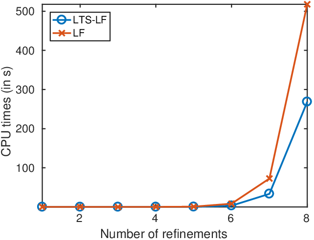
Refer to caption
Figure 3: Comparison of run times between LTS-LF and standard LF vs. number of global refinements with constant coarse/fine mesh size ratio p=4p=4.

Acknowledgements

We thank Loredana Gaudio for useful comments and suggestions during the initial stages of this work and Maximillian Matthäus for his Matlab program.

Appendix A Some Auxiliary Estimates

Lemma 19

For p≥2p\geq 2 let αjp\alpha_{j}^{p}, j=1,…,p−1j=1,\dots,p-1, be recursively defined as in (11). Then, the constants αjp\alpha_{j}^{p} are given by

αjp=∏ℓ=0j(ℓ2−p2)(2​j+2)!,1≤j≤p−1,p≥2\alpha_{j}^{p}=\frac{{\displaystyle\prod\limits_{\ell=0}^{j}}\left(\ell^{2}-p^{2}\right)}{(2j+2)!},\qquad 1\leq j\leq p-1,\quad p\geq 2 (72)

Moreover, for κ∈[0,4​p2]\kappa\in\left[0,4p^{2}\right] it holds

|2p2​∑j=1p−1αjp​(κp2)j|≤κ12and ​|2p2​∑j=1p−1αjp​(κp2)j−1|≤p2−112.\left|\frac{2}{p^{2}}\sum_{j=1}^{p-1}\alpha_{j}^{p}\left(\frac{\kappa}{p^{2}}\right)^{j}\right|\leq\frac{\kappa}{12}\quad\text{and\hskip 10.22217pt}\left|\frac{2}{p^{2}}\sum_{j=1}^{p-1}\alpha_{j}^{p}\left(\frac{\kappa}{p^{2}}\right)^{j-1}\right|\leq\frac{p^{2}-1}{12}.

Proof. To show that the constants αjp\alpha_{j}^{p} are in fact given by (72), we first use the identity

p⁡(p+j)​(p+j−1)​…​(p+1)​p​(p−1)​…​(p−j+1)​(p−j)=∏ℓ=0j(p2−ℓ2)p(p+j)(p+j-1)\dots(p+1)p(p-1)\dots(p-j+1)(p-j)={\displaystyle\prod\limits_{\ell=0}^{j}}\left(p^{2}-\ell^{2}\right) (73)

to rewrite (72) as

αjp=(−1)j+1​p​(p+j)!(p−j−1)!​(2​j+2)!.\alpha_{j}^{p}=\frac{\left(-1\right)^{j+1}p\left(p+j\right)!}{\left(p-j-1\right)!\left(2j+2\right)!}. (74)

By using (74) it is then straightforward to verify that αjp\alpha_{j}^{p} satisfies the recursive definition in (11).

Next, one proves by induction that

∑j=1p−1αjp​xj\displaystyle\sum_{j=1}^{p-1}\alpha_{j}^{p}x^{j} =p22+Tp​(1−x2)−1x\displaystyle=\frac{p^{2}}{2}+\frac{T_{p}\left(1-\frac{x}{2}\right)-1}{x}
∑j=1p−1αjp​xj−1\displaystyle\sum_{j=1}^{p-1}\alpha_{j}^{p}x^{j-1} =p2​x+2​Tp​(1−x2)−22​x2.\displaystyle=\frac{p^{2}x+2\,T_{p}\left(1-\frac{x}{2}\right)-2}{2x^{2}}.

with the Čebyšev polynomials TpT_{p} of the first kind. We recall that

Tp(m)​(1)=∏ℓ=0m−1(p2−ℓ2)(2​ℓ+1)and ​‖Tp(m)‖L∞​([−1,1])=Tp(m)​(1),T_{p}^{\left(m\right)}\left(1\right)={\displaystyle\prod\limits_{\ell=0}^{m-1}}\frac{\left(p^{2}-\ell^{2}\right)}{\left(2\ell+1\right)}\qquad\text{and\quad}\left\|T_{p}^{(m)}\right\|_{L^{\infty}\left(\left[-1,1\right]\right)}=T_{p}^{\left(m\right)}\left(1\right), (75)

where the first relation follows from [43, (1.97)] and the second one from [43, Theorem 2.24], see also [44, Corollary 7.3.1].

Now, let x=κ/p2x=\kappa/p^{2}. The condition κ∈[0,4​p2]\kappa\in\left[0,4p^{2}\right] implies [1−x2,1]⊂[−1,1]\left[1-\frac{x}{2},1\right]\subset\left[-1,1\right]. Hence, a Taylor argument shows that there exists ξ∈[−1,1]\xi\in\left[-1,1\right] such that

|∑j=1p−1αjp​xj|\displaystyle\left|\sum_{j=1}^{p-1}\alpha_{j}^{p}x^{j}\right| =|p22+Tp​(1)−x2​Tp′​(1)+x28​Tp′′​(ξ)−1x|\displaystyle=\left|\frac{p^{2}}{2}+\frac{T_{p}\left(1\right)-\frac{x}{2}T_{p}^{\prime}\left(1\right)+\frac{x^{2}}{8}T_{p}^{\prime\prime}\left(\xi\right)-1}{x}\right|
=|x8​Tp′′​(ξ)|≤p2​(p2−1)24​x=p2−124​κ,\displaystyle=\left|\frac{x}{8}T_{p}^{\prime\prime}\left(\xi\right)\right|\leq\frac{p^{2}\left(p^{2}-1\right)}{24}x=\frac{p^{2}-1}{24}\kappa, (76)

where we have also used (75). Similarly, we get

|∑j=1p−1αjp​xj−1|\displaystyle\left|\sum_{j=1}^{p-1}\alpha_{j}^{p}x^{j-1}\right| =|p2​x+2​(Tp​(1)−x2​Tp′​(1)+x28​Tp′′​(ξ))−22​x2|\displaystyle=\left|\frac{p^{2}x+2\left(T_{p}\left(1\right)-\frac{x}{2}T_{p}^{\prime}\left(1\right)+\frac{x^{2}}{8}T_{p}^{\prime\prime}\left(\xi\right)\right)-2}{2x^{2}}\right|
=|p2​x+2​(1−x​p22+x28​Tp′′​(ξ))−22​x2|=18​|Tp′′​(ξ)|≤p2​(p2−1)24.\displaystyle=\left|\frac{p^{2}x+2\left(1-\frac{xp^{2}}{2}+\frac{x^{2}}{8}T_{p}^{\prime\prime}\left(\xi\right)\right)-2}{2x^{2}}\right|=\frac{1}{8}\left|T_{p}^{\prime\prime}\left(\xi\right)\right|\leq\frac{p^{2}\left(p^{2}-1\right)}{24}.


References

  • [1] D. N. Arnold, F. Brezzi, B. Cockburn, and L. D. Marini. Unified analysis of discontinuous Galerkin methods for elliptic problems. SIAM J. Numer. Anal., 39(5):1749–1779, 2001/02.
  • [2] U. Ascher, S. Ruuth, and B. Wetton. Implicit-explicit methods for time-dependent partial differential equations. SIAM J. Numer. Anal., 32(3):797–823, 1995.
  • [3] G. A. Baker. Error estimates for finite element methods for second order hyperbolic equations. SIAM J. Numer. Anal., 13(4):564–576, 1976.
  • [4] E. Bécache, P. Joly, and J. Rodríguez. Space-time mesh refinement for elastodynamics. Numerical results. Comput. Methods Appl. Mech. Engrg., 194(2-5):355–366, 2005.
  • [5] M. Berger and J. Oliger. Adaptive mesh refinement for hyperbolic partial differential equations. J. Comput. Phys., 53:484–512, 1984.
  • [6] S. C. Brenner and L. R. Scott. The mathematical theory of finite element methods, volume 15. Springer, New York, third edition, 2008.
  • [7] C. Canuto, M. Hussaini, A. Quateroni, and T. Zang, editors. Spectral Methods: Fundamentals in Single Domains. Springer–Verlag, 2006.
  • [8] P. Ciarlet. The finite element method for elliptic problems. North-Holland, 1987.
  • [9] B. Cockburn, G. Karniadakis, and C.-W. Shu, editors. Spectral/hp element for Cfd. Oxford University Press, 2005.
  • [10] G. Cohen, P. Joly, J. Roberts, and N. Tordjman. Higher order triangular finite elements with mass lumping for the wave equation. SIAM J. Numer. Anal., 38:2047–2078, 2001.
  • [11] F. Collino, T. Fouquet, and P. Joly. A conservative space-time mesh refinement method for the 1-D wave equation. I. Construction. Numer. Math., 95(2):197–221, 2003.
  • [12] F. Collino, T. Fouquet, and P. Joly. A conservative space-time mesh refinement method for the 1-D wave equation. II. Analysis. Numer. Math., 95(2):223–251, 2003.
  • [13] F. Collino, T. Fouquet, and P. Joly. Conservative space-time mesh refinement methods for the FDTD solution of Maxwell’s equations. J. Comput. Phys., 211(1):9–35, 2006.
  • [14] E. Constantinescu and A. Sandu. Multirate time stepping methods for hyperbolic conservation laws. SIAM J. Sci. Comput., 33:239–278, 2007.
  • [15] E. Constantinescu and A. Sandu. Multirate explicit Adams methods for time integration of conservation laws. SIAM J. Sci. Comput., 38:229–249, 2009.
  • [16] A. Demirel, J. Niegemann, K. Busch, and M. Hochbruck. Efficient Multiple Time-Stepping Algorithms of Higher Order. J. Comput. Phys., 285:133–148, 2015.
  • [17] S. Descombes, S. Lantéri, and L. Moya. Locally implicit discontinuous Galerkin method for time domain electromagnetics. J. Sci. Comp., 56:190–218, 2013.
  • [18] J. Diaz and M. J. Grote. Energy conserving explicit local time-stepping for second-order wave equations. SIAM J. Sci. Comput., 31:1985–2014, 2009.
  • [19] J. Diaz and M. J. Grote. Multi-level explicit local time-stepping methods for second-order wave equations. Comput. Methods Appl. Mech. Engrg., 291:240–265, 2015.
  • [20] V. Dolean, H. Fahs, L. Fezoui, and S. Lanteri. Locally implicit discontinuous Galerkin method for time domain electromagnetics. J. Comput. Phys., 229:512–526, 2010.
  • [21] M. Dumbser, M. Käser, and E. Toro. An arbitrary high-order discontinuous Galerkin method for elastic waves on unstructured meshes – V. local time stepping and pp-adaptivity. Geophys. J. Int., 171:695–717, 2007.
  • [22] T. Dupont. L2{L}^{2}–Estimates for Galerkin Methods for Second Order Hyperbolic Equations. SIAM J. Numer. Anal., 10(5):880–889, 1973.
  • [23] J. Flaherty, R. Loy, M.S.Shephard, B. Szymanski, J. Teresco, and L. Ziantz. Adaptive local refinement with octree load-balancing for the parallel solution of three-dimensional conservation laws. J. Paral. Distrib. Comp., 47:139–152, 1997.
  • [24] C. W. Gear and D. R. Wells. Multirate linear multistep methods. BIT, 24:484–502, 1984.
  • [25] M. J. Grote, M. Mehlin, and T. Mitkova. Runge-Kutta-based explicit local time-stepping methods for wave propagation. SIAM J. Sci. Comput., 37(2):A747–A775, 2015.
  • [26] M. J. Grote and T. Mitkova. Explicit local time-stepping methods for Maxwell’s equations. J. Comput. Appl. Math., 234(12):3283–3302, 2010.
  • [27] M. J. Grote and T. Mitkova. High-order explicit local time-stepping methods for damped wave equations. J. Comput. Appl. Math., 239:270–289, 2013.
  • [28] M. J. Grote, A. Schneebeli, and D. Schötzau. Discontinuous Galerkin finite element method for the wave equation. SIAM J. Numer. Anal., 44(6):2408–2431, 2006.
  • [29] M. Hochbruck and A. Ostermann. Exponential multistep methods of Adams type. BIT, 51:889–908, 2011.
  • [30] M. Hochbruck and A. Sturm. Error analysis of a second-order locally implicit method for linear Maxwell’s equations. SIAM Journal on Numerical Analysis, 54(5):3167–3191, 2016.
  • [31] W. Hundsdorfer and J. Verwer. Numerical solution of time-dependent advection-diffusion-reaction equations, volume 33 of Springer Series in Computational Mathematics. Springer-Verlag, Berlin, 2003.
  • [32] P. Joly and J. Rodríguez. An error analysis of conservative space-time mesh refinement methods for the one-dimensional wave equation. SIAM J. Numer. Anal., 43(2):825–859 (electronic), 2005.
  • [33] A. Kanevsky, M. H. Carpenter, D. Gottlieb, and J. S. Hesthaven. Application of implicit-explicit high order Runge-Kutta methods to discontinuous Galerkin schemes. J. Comput. Phys., 225:1753–1781, 2007.
  • [34] J. Lions and E. Magenes. Non-Homogeneous Boundary Value Problems and Applications. Springer-Verlag, Berlin, 1972.
  • [35] F. Lörcher, G. Gassner, and C.-D. Munz. A discontinuous Galerkin scheme based on a space-time expansion. I. Inviscid compressible flow in one space dimension. J. Sc. Comp., 32:175–199, 2007.
  • [36] S. Minisini, E. Zhebel, A. Kononov, and W. A. Mulder. Local time stepping with the discontinuous Galerkin method for wave propagation in 3D heterogeneous media. Geophysics, 78:T67–T77, 2013.
  • [37] E. Montseny, S. Pernet, X. Ferriéres, and G. Cohen. Dissipative terms and local time-stepping improvements in a spatial high order Discontinuous Galerkin scheme for the time-domain Maxwell’s equations. J. Comput. Phys., 227:6795–6820, 2008.
  • [38] W. Mulder. Higher-order mass-lumped finite elements for the wave equation. J. Comput. Acoust., 09:671–680, 2001.
  • [39] F. L. Müller and C. Schwab. Finite elements with mesh refinement for wave equations in polygons. J. Comput. Appl. Math., 283:163–181, 2015.
  • [40] F. L. Müller and C. Schwab. Finite elements with mesh refinement for elastic wave propagation in polygons. Math. Meth. Appl. Sci., 39:527–542, 2016.
  • [41] S. Piperno. Symplectic local time-stepping in non-dissipative DGTD methods applied to wave propagation problems. M2AN Math. Model. Numer. Anal., 40(5):815–841, 2006.
  • [42] M. Rietmann, M. J. Grote, D. Peter, and O. Schenk. Newmark local time stepping on high-performance computing architectures. J. Comput. Phys., 334:308–326, 2017.
  • [43] T. J. Rivlin. Chebyshev Polynomials. Wiley, New York, 1974.
  • [44] S. Sauter and C. Schwab. Boundary Element Methods. Springer, Heidelberg, 2010.
  • [45] J. Stoer and R. Bulirsch. Numerische Mathematik. Springer-Verlag, Heidelberg, 3 edition, 1990.
  • [46] A. Taube, M. Dumbser, C.-D. Munz, and R. Schneider. A high-order discontinuous Galerkin method with time-accurate local time stepping for the Maxwell equations. Int. J. Numer. Model., 22:77–103, 2009.
  • [47] J. Verwer. Convergence and component splitting for the Crank-Nicolson-leap-frog integration method. Technical Report Technical Report MAS-E0902, CWI, 2009.