跳到论文正文
W Papers独立论文阅读器 arXiv:1703.07924 论文正文 计算阅读时间 · 0%
引用这篇论文根据当前论文元数据生成,正式投稿前建议核对。


License: arXiv.org perpetual non-exclusive license
arXiv:1703.07924v2 [math-ph] 29 Mar 2017

Symmetric functions and wavefunctions of the six-vertex model by Izergin-Korepin analysis

Kohei Motegi ††thanks: E-mail: kmoteg0@kaiyodai.ac.jp Affiliation: Faculty of Marine Technology, Tokyo University of Marine Science and Technology, Affiliation: Etchujima 2-1-6, Koto-Ku, Tokyo, 135-8533, Japan
August 24, 2026
Abstract

We analyze wavefunctions of the six-vertex model by extending the Izergin-Korepin analysis on the domain wall boundary partition functions. We particularly focus on the case with triangular boundary. By using the Uq​(s​l2)U_{q}(sl_{2}) RR-matrix and a special class of the triangular KK-matrix, we first introduce an analogue of the wavefunctions of the integrable six-vertex model with triangular boundary. We first give a characterization of the wavefunctions by extending our recent work of the Izergin-Korepin analysis of the domain wall boundary partition function with triangular boundary, and then determine the explicit form of the symmetric functions representing the wavefunctions by showing that it satisfies all the required properties. We also illustrate the Izergin-Korepin analysis for the case of ordinary wavefunctions as it is the basic case.

1 Introduction

The most fundamental and important objects in statistical physics are partition functions. Exact computations of partition functions have great impacts in mathematical physics and mathematics. The field of integrable lattice models [1, 2, 3, 4] offers us chances to compute partition functions exactly, and have stimulated the advances of representation theory and algebraic combinatorics. One of the most basic partition functions called the domain wall boundary partition function [5, 6] has become famous in the field of algebraic combinatorics in 1990s, since its determinant form was realized to be a certain generalization of the generating function of the enumeration of the alternating sign matrix [7, 8, 9, 10]. Relation with classical integrable models [11], orthogonal polynomials [12], asymptotics in the thermodynamic limit [13, 14, 15] were also investigated.

Various variations of the domain wall boundary partition functions were introduced. One of the motivations of studying these variations comes from the expectation that investigating variations leads us to applications to the variations of the enumeration of the alternating sign matrices [9, 10, 16, 17, 18].

In recent years, more generic partition functions which we shall call as the wavefunctions are attracting attention. The domain wall boundary partition function can be regarded as the simplest case of the wavefunctions. By studying the wavefunctions of various integrable models and various boundary conditions, it has been recognized that their explicit forms are nothing but symmetric functions such as the Schur, Hall-Littlewood, Grothendieck polynoimals and their deformations. As one of the applications of these integrable model realizations of symmetric polynomials, we can discover various new algebraic combinatorial identities which give substantial generalizations of the Cauchy, dual Cauchy, Littlewood, Tokuyama formulae and the Littlewood-Richardson coefficients. There are now a lot of papers on this subject. See [19, 20, 21, 22, 23, 24, 25, 26, 27, 28, 29, 30, 31, 32] for examples which investigate symmetric functions by using the XXZ model and the qq-boson model, and [33, 34, 35, 36, 37, 38] by using the free-fermion model in an external field .

In this paper, we introduce and study an analogue of the wavefunctions. We investigate the wavefunctions with triangular boundary. The main motivation of introducing this object is to generalize combinatorial objects such as the non-intersecting lattice paths and excited Young diagrams in Schubert calculus [39, 40, 41, 42, 43]. By translating those combinatorial objects into the language of integrable lattice models, one finds that those combinatorial objects use the q=0q=0 degeneration of the Uq​(s​l2)U_{q}(sl_{2}) RR-matrix as bulk weights. From the point of view of quantum integrability, it is natural to have the following feeling: why don’t we use the Uq​(s​l2)U_{q}(sl_{2}) RR-matrix itself as bulk weights? In our very recent work [44], we analyzed the domain wall boundary partition function with triangular boundary which is the very first step, and determined its explicit expression as a certain symmetric function. The Izergin-Korepin analysis [5, 6, 48] was crucial to get the explicit form. In this paper, we extend the Izergin-Korepin analysis to the wavefunctions, and determine the explicit form which is an extension of the symmetric function representing the domain wall boundary partition function.

This paper is organized as follows. In the next section, we first list the Uq​(s​l2)U_{q}(sl_{2}) RR-matrix and the triangular KK-matrix which we use in this paper. Using these RR-matrix and KK-matrix, we introduce the wavefunctions with triangular boundary in section 3. In section 4, we make the Izergin-Korepin analysis and list the properties needed to determine the explicit form of the wavefunctions. In section 5, we present the symmetric function which gives the explicit form of the wavefunctions by showing that it satisfies all the required properties. Section 6 is devoted to conclusion. We illustrate the Izergin-Korepin analysis to the ordinary wavefunctions in the Apeendix.

2 The six-vertex model

In this section, we introduce the Uq​(s​l2)U_{q}(sl_{2}) RR-matrix and the KK-matrix which will be used as local bulk and boundary pieces of the wavefunctions with triangular boundary which will be introduced in the next section.

The most fundamental objects in integrable lattice models are the RR-matrix. In this paper, we use the following Uq​(s​l2)U_{q}(sl_{2}) RR-matrix [45, 46]

Ra​b​(u,w)=(u−t​w0000t⁡(u−w)(1−t)​u00(1−t)​wu−w0000u−t​w),\displaystyle R_{ab}(u,w)=\left(\begin{array}[]{cccc}u-tw&0&0&0\\ 0&t(u-w)&(1-t)u&0\\ 0&(1-t)w&u-w&0\\ 0&0&0&u-tw\end{array}\right),

acting on the tensor product Wa⊗WbW_{a}\otimes W_{b} of the complex two-dimensional space WaW_{a}. Let us denote the orthonormal basis of WaW_{a} and its dual as {|0⟩a,|1⟩a}\{|0\rangle_{a},|1\rangle_{a}\} and {⟨0|,⟨1|}aa\{{}_{a}\langle 0|,{}_{a}\langle 1|\}, and the matrix elements of the RR-matrix as ⟨γ|⟨δ|Ra​b(u,w)|α⟩ab|β⟩ba=[Ra​b(u,w)]α​βγ​δ{}_{a}\langle\gamma|{}_{b}\langle\delta|R_{ab}(u,w)|\alpha\rangle_{a}|\beta\rangle_{b}=[R_{ab}(u,w)]_{\alpha\beta}^{\gamma\delta}. The matrix elements of the RR-matrix are explicitly given as

⟨0|⟨0|Ra​b(u,w)|0⟩ab|0⟩ba\displaystyle{}_{a}\langle 0|{}_{b}\langle 0|R_{ab}(u,w)|0\rangle_{a}|0\rangle_{b} =u−t​w,\displaystyle=u-tw, (2.6)
⟨0|⟨1|Ra​b(u,w)|0⟩ab|1⟩ba\displaystyle{}_{a}\langle 0|{}_{b}\langle 1|R_{ab}(u,w)|0\rangle_{a}|1\rangle_{b} =t⁡(u−w),\displaystyle=t(u-w), (2.7)
⟨0|⟨1|Ra​b(u,w)|1⟩ab|0⟩ba\displaystyle{}_{a}\langle 0|{}_{b}\langle 1|R_{ab}(u,w)|1\rangle_{a}|0\rangle_{b} =(1−t)​u,\displaystyle=(1-t)u, (2.8)
⟨1|⟨0|Ra​b(u,w)|0⟩ab|1⟩ba\displaystyle{}_{a}\langle 1|{}_{b}\langle 0|R_{ab}(u,w)|0\rangle_{a}|1\rangle_{b} =(1−t)​w,\displaystyle=(1-t)w, (2.9)
⟨1|⟨0|Ra​b(u,w)|1⟩ab|0⟩ba\displaystyle{}_{a}\langle 1|{}_{b}\langle 0|R_{ab}(u,w)|1\rangle_{a}|0\rangle_{b} =u−w,\displaystyle=u-w, (2.10)
⟨1|⟨1|Ra​b(u,w)|1⟩ab|1⟩ba\displaystyle{}_{a}\langle 1|{}_{b}\langle 1|R_{ab}(u,w)|1\rangle_{a}|1\rangle_{b} =u−t​w.\displaystyle=u-tw. (2.11)

The RR-matrix (2) satsifies the Yang-Baxter relation

Ra​b​(u,v)​Ra​c​(u,w)​Rb​c​(v,w)=Rb​c​(v,w)​Ra​c​(u,w)​Ra​b​(u,v),\displaystyle R_{ab}(u,v)R_{ac}(u,w)R_{bc}(v,w)=R_{bc}(v,w)R_{ac}(u,w)R_{ab}(u,v), (2.12)

acting on Wa⊗Wb⊗WcW_{a}\otimes W_{b}\otimes W_{c}.

See Figures 1 and 2 for the graphical description of the RR-matrix and the Yang-Baxter relation used in this paper. The RR-matrices have origins in statistical physics, and |0⟩|0\rangle or its dual ⟨0|\langle 0| can be regarded as a spin up state, while |1⟩|1\rangle or its dual ⟨1|\langle 1| can be interpretted as a spin down state from the point of view of statistical physics. We sometimes use the terms spin up states (up spins) and spin down states (down spins) to describe states constructed from |0⟩|0\rangle, ⟨0|\langle 0|, |1⟩|1\rangle and ⟨1|\langle 1| since they are convenient for the description of the states.

Refer to caption
Figure 1: The RR-matrix R⁡(u,w)R(u,w) (2). We regard that each line is a representation space and carries a spectral parameter. In this picture, the horizontal line carries a spectral parameter uu, while the vertical line carries ww.
Refer to caption
Figure 2: The Yang-Baxter relation (2.12). The left and right figure represents Ra​b​(u,v)​Ra​c​(u,w)​Rb​c​(v,w)R_{ab}(u,v)R_{ac}(u,w)R_{bc}(v,w) and Rb​c​(v,w)​Ra​c​(u,w)​Ra​b​(u,v)R_{bc}(v,w)R_{ac}(u,w)R_{ab}(u,v) respectively.
Refer to caption
Figure 3: The KK-matrix K⁡(u)K(u) (2). We regard that the horizontal line carries a spectral parameter uu, while the vertical line carries its inverse u−1u^{-1}.
Refer to caption
Figure 4: The reflection equation (2.20). The left and right figure represents Rb​a​(u/w)​Kb​(u)​Ra​b​(u​w)​Ka​(w)R_{ba}(u/w)K_{b}(u)R_{ab}(uw)K_{a}(w) and Ka​(w)​Rb​a​(u​w)​Kb​(u)​Ra​b​(u/w)K_{a}(w)R_{ba}(uw)K_{b}(u)R_{ab}(u/w) respectively.

We also introduce the triangular KK-matrix acting on WaW_{a} (see Figure 3)

Ka​(u)=(B​u−A0u−u−1B​u−1−A),\displaystyle K_{a}(u)=\left(\begin{array}[]{cc}Bu-A&0\\ u-u^{-1}&Bu^{-1}-A\\ \end{array}\right),

where AA and BB are arbitrary complex parameters. The matrix elements are explicitly given by

⟨0|Ka(u)|0⟩aa\displaystyle{}_{a}\langle 0|K_{a}(u)|0\rangle_{a} =B​u−A,\displaystyle=Bu-A, (2.16)
⟨0|Ka(u)|1⟩aa\displaystyle{}_{a}\langle 0|K_{a}(u)|1\rangle_{a} =0,\displaystyle=0, (2.17)
⟨1|Ka(u)|1⟩aa\displaystyle{}_{a}\langle 1|K_{a}(u)|1\rangle_{a} =B​u−1−A,\displaystyle=Bu^{-1}-A, (2.18)
⟨1|Ka(u)|0⟩aa\displaystyle{}_{a}\langle 1|K_{a}(u)|0\rangle_{a} =u−u−1.\displaystyle=u-u^{-1}. (2.19)

The KK-matrix (2) together with the RR-matrix satisfy the following relation

Rb​a​(u/w)​Kb​(u)​Ra​b​(u​w)​Ka​(w)=Ka​(w)​Rb​a​(u​w)​Kb​(u)​Ra​b​(u/w),\displaystyle R_{ba}(u/w)K_{b}(u)R_{ab}(uw)K_{a}(w)=K_{a}(w)R_{ba}(uw)K_{b}(u)R_{ab}(u/w), (2.20)

which is called as the reflection equation or the boundary Yang-Baxter equation [47]. The reflection equation ensures the integrability at the boundary, and we use this particular KK-matrix as local pieces of the wavefunctions at the boundary. Note that (2) can be regarded as a specialization of the full KK-matrix which satisfies the reflection equation (2.20). See Figure 4 for the grahical representation of the reflection equation.

For later convenience, we finally define in this section the following Pauli spin operators σ+\sigma^{+} and σ−\sigma^{-} as operators acting on the (dual) orthonomal basis as

σ+​|1⟩=|0⟩,σ+​|0⟩=0,⟨0|​σ+=⟨1|,⟨1|​σ+=0,\displaystyle\sigma^{+}|1\rangle=|0\rangle,\ \sigma^{+}|0\rangle=0,\ \langle 0|\sigma^{+}=\langle 1|,\ \langle 1|\sigma^{+}=0, (2.21)
σ−​|0⟩=|1⟩,σ−​|1⟩=0,⟨1|​σ−=⟨0|,⟨0|​σ−=0.\displaystyle\sigma^{-}|0\rangle=|1\rangle,\ \sigma^{-}|1\rangle=0,\ \langle 1|\sigma^{-}=\langle 0|,\ \langle 0|\sigma^{-}=0. (2.22)
Refer to caption
Figure 5: The monodromy matrix Tj(u1,…,uj|w1,…,wN)T_{j}(u_{1},\dots,u_{j}|w_{1},\dots,w_{N}) (3.1).

3 Wavefunctions

To introduce the wavefunctions with triangular boundary, we introduce the tensor product of the Fock spaces W−n⊗⋯⊗W−1⊗W1⊗⋯⊗WNW_{-n}\otimes\cdots\otimes W_{-1}\otimes W_{1}\otimes\cdots\otimes W_{N}. Note that here we do not introduce a Fock space named W0W_{0}.

We next define the following monodromy matrix Tj(u1,…,uj|w1,…,wN)T_{j}(u_{1},\dots,u_{j}|w_{1},\dots,w_{N}), j=1,…,nj=1,\dots,n using the RR-matrix and the KK-matrix as

Tj(u1,…,uj|w1,…,wN)\displaystyle T_{j}(u_{1},\dots,u_{j}|w_{1},\dots,w_{N})
=\displaystyle= R−j,N(uj,wN)⋯R−j,1(uj,w1)R−j,−1(uju1,1)⋯R−j,−j+1(ujuj−1,1)K−j(uj),\displaystyle R_{-j,N}(u_{j},w_{N})\cdots R_{-j,1}(u_{j},w_{1})R_{-j,-1}(u_{j}u_{1},1)\cdots R_{-j,-j+1}(u_{j}u_{j-1},1)K_{-j}(u_{j}), (3.1)

which acts on W−j⊗⋯⊗W−1⊗W1⊗⋯⊗WNW_{-j}\otimes\cdots\otimes W_{-1}\otimes W_{1}\otimes\cdots\otimes W_{N}. See Figure 5 for a pictorial description of (3.1).

Next, we define the state vector |ΨN,n(u1,…,un|w1,…,wN)⟩∈W1⊗⋯⊗WN|\Psi_{N,n}(u_{1},\dots,u_{n}|w_{1},\dots,w_{N})\rangle\in W_{1}\otimes\cdots\otimes W_{N} by using the monodromy matrix Tj(u1,…,uj|w1,…,wN)T_{j}(u_{1},\dots,u_{j}|w_{1},\dots,w_{N}) as

|ΨN,n(u1,…,un|w1,…,wN)⟩\displaystyle|\Psi_{N,n}(u_{1},\dots,u_{n}|w_{1},\dots,w_{N})\rangle
=\displaystyle= ⟨0n|T1(u1|w1,…,wN)⋯Tn(u1,…,un|w1,…,wN)|Ω⟩n+N,\displaystyle\langle 0^{n}|T_{1}(u_{1}|w_{1},\dots,w_{N})\cdots T_{n}(u_{1},\dots,u_{n}|w_{1},\dots,w_{N})|\Omega\rangle_{n+N}, (3.2)

where the states ⟨0n|\langle 0^{n}| and |Ω⟩n+N|\Omega\rangle_{n+N} are defined as

⟨0n|\displaystyle\langle 0^{n}| =⟨0|⊗⋯⊗⟨0|,−1−n\displaystyle={}_{-n}\langle 0|\otimes\cdots\otimes{}_{-1}\langle 0|, (3.3)
|Ω⟩n+N\displaystyle|\Omega\rangle_{n+N} =|0⟩−n⊗⋯⊗|0⟩−1⊗|0⟩1⊗⋯⊗|0⟩N.\displaystyle=|0\rangle_{-n}\otimes\cdots\otimes|0\rangle_{-1}\otimes|0\rangle_{1}\otimes\cdots\otimes|0\rangle_{N}. (3.4)

This is an analogue of the off-shell Bethe vector. We remark that there is a big difference on the properties between the state vector (3.2) and the ordinary off-shell Bethe vector. The ordinary off-shell Bethe vector of the six-vertex model (and its degeneration to the five-vertex model) is constructed from the multiple action of the so-called BB-operators on the vacuum state, and one BB-operator always creates one dowm spin, hence the ordinary off-shell Bethe vector constructed from nn layers of BB-operators gives an nn-down spin state. However, the state vector (3.2) constructed from nn layers Tj(u1,…,uj|w1,…,wN)T_{j}(u_{1},\dots,u_{j}|w_{1},\dots,w_{N}), j=1,⋯,nj=1,\cdots,n do not always give an nn-down spin state.

Keeping this in mind, let us now introduce an analogue of the wavefunctions with triangular boundary. We first introduce the following dual spin states

⟨x1⋯xm|\displaystyle\langle x_{1}\cdots x_{m}| =(1⟨0|⊗⋯⊗⟨0|)N∏j=1mσxj+∈W1∗⊗⋯⊗WN∗,\displaystyle=(_{1}\langle 0|\otimes\cdots\otimes{}_{N}\langle 0|)\prod_{j=1}^{m}\sigma^{+}_{x_{j}}\in W_{1}^{*}\otimes\cdots\otimes W_{N}^{*}, (3.5)

which are states labelling the configurations of down spins 1≤x1<x2<⋯<xm≤N1\leq x_{1}<x_{2}<\cdots<x_{m}\leq N. Wa∗W_{a}^{*} means the dual space of WaW_{a}.

Refer to caption
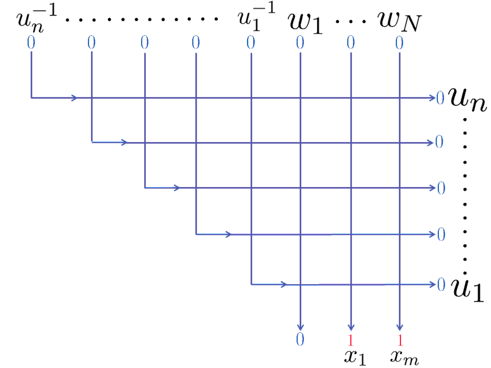
Figure 6: The wavefunctions with triangular boundary WN,n,m(u1,…,un|w1,…,wN|x1,…,xm)W_{N,n,m}(u_{1},\dots,u_{n}|w_{1},\dots,w_{N}|x_{1},\dots,x_{m}) (3.7). This figure illustrates the case N=3,n=5,m=2,x1=2,x2=3N=3,\ n=5,\ m=2,\ x_{1}=2,\ x_{2}=3.

Now we define the wavefunctions with triangular boundary
WN,n,m(u1,…,un|w1,…,wN|x1,…,xm)W_{N,n,m}(u_{1},\dots,u_{n}|w_{1},\dots,w_{N}|x_{1},\dots,x_{m}) as the inner product between the state vector
|ΨN,n(u1,…,un|w1,…,wN)⟩|\Psi_{N,n}(u_{1},\dots,u_{n}|w_{1},\dots,w_{N})\rangle and the mm-down spin state ⟨x1⋯xm|\langle x_{1}\cdots x_{m}| as

WN,n,m(u1,…,un|w1,…,wN|x1,…,xm)=⟨x1⋯xm|ΨN,n(u1,…,un|w1,…,wN)⟩.\displaystyle W_{N,n,m}(u_{1},\dots,u_{n}|w_{1},\dots,w_{N}|x_{1},\dots,x_{m})=\langle x_{1}\cdots x_{m}|\Psi_{N,n}(u_{1},\dots,u_{n}|w_{1},\dots,w_{N})\rangle. (3.6)

The wavefunctions (3.6) can be seen as an extension of the domain wall boundary partition function with triangular boundary

Zn,m(u1,…,un|w1,…,wm)\displaystyle Z_{n,m}(u_{1},\dots,u_{n}|w_{1},\dots,w_{m})
=\displaystyle= ⟨0n1m|T1(u1|w1,…,wm)⋯Tn(u1,…,un|w1,…,wm)|Ω⟩n+m,\displaystyle\langle 0^{n}1^{m}|T_{1}(u_{1}|w_{1},\dots,w_{m})\cdots T_{n}(u_{1},\dots,u_{n}|w_{1},\dots,w_{m})|\Omega\rangle_{n+m}, (3.7)
⟨0n​1m|=\displaystyle\langle 0^{n}1^{m}|= ⟨0|⊗⋯⊗⟨0|⊗⟨1|⊗⋯⊗⟨1|,m1−1−n\displaystyle{}_{-n}\langle 0|\otimes\cdots\otimes{}_{-1}\langle 0|\otimes{}_{1}\langle 1|\otimes\cdots\otimes{}_{m}\langle 1|, (3.8)

which we introduced in our last paper [44], since the special case N=mN=m, xj=jx_{j}=j, j=1,⋯,mj=1,\cdots,m of the wavefunctions (3.6) is nothing but the domain wall boundary partition function

Wm,n,m(u1,…,un|w1,…,wm|1,…,m)=Zn,m(u1,…,un|w1,…,wm).\displaystyle W_{m,n,m}(u_{1},\dots,u_{n}|w_{1},\dots,w_{m}|1,\dots,m)=Z_{n,m}(u_{1},\dots,u_{n}|w_{1},\dots,w_{m}). (3.9)

The wavefunctions WN,n,m(u1,…,un|w1,…,wN|x1,…,xm)W_{N,n,m}(u_{1},\dots,u_{n}|w_{1},\dots,w_{N}|x_{1},\dots,x_{m}) is a symmetric function with respect to the spectral parameters {u}n\{u\}_{n} which can be shown in the same way we showed for the case of the domain wall boundary partition function [44] by the so-called railroad argument using the Yang-Baxter relation and the reflection equation. Thus, we sometimes abbreviate WN,n,m(u1,…,un|w1,…,wN|x1,…,xm)W_{N,n,m}(u_{1},\dots,u_{n}|w_{1},\dots,w_{N}|x_{1},\dots,x_{m}) as
WN,n,m({u}n|w1,…,wN|x1,…,xm)W_{N,n,m}(\{u\}_{n}|w_{1},\dots,w_{N}|x_{1},\dots,x_{m}) where {u}n\{u\}_{n} means {u1,…,un}\{u_{1},\dots,u_{n}\} as a set. See Figure 6 for the graphical description of the wavefunctions WN,n,m(u1,…,un|w1,…,wN|x1,…,xm)W_{N,n,m}(u_{1},\dots,u_{n}|w_{1},\dots,w_{N}|x_{1},\dots,x_{m}).

Refer to caption
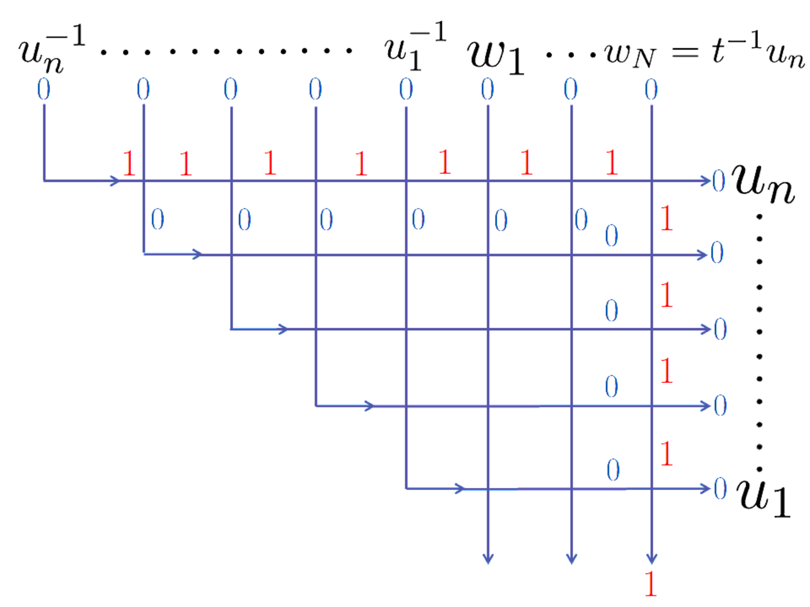
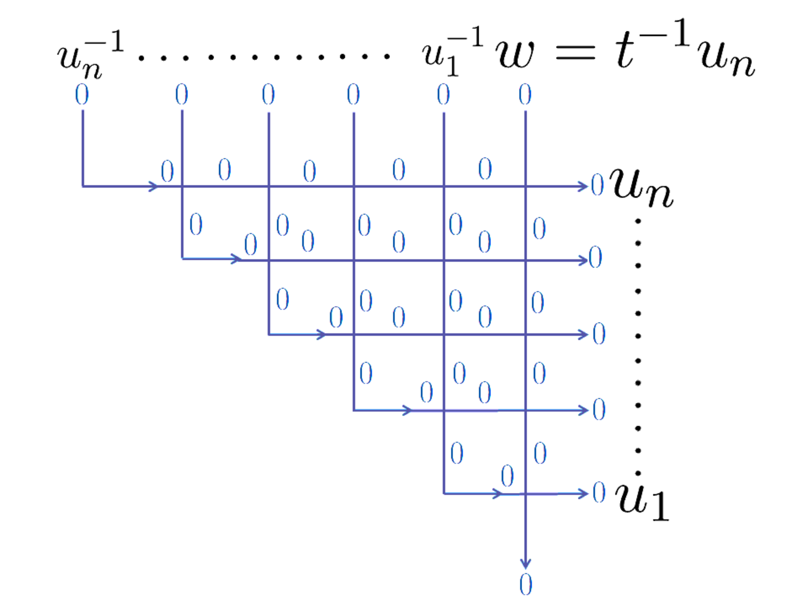
Figure 7: The recursion relation WN,n,m(u1,…,un|w1,…,wN|x1,…,xm)W_{N,n,m}(u_{1},\dots,u_{n}|w_{1},\dots,w_{N}|x_{1},\dots,x_{m}), xm=Nx_{m}=N evaluated at wN=t−1​unw_{N}=t^{-1}u_{n} (4.1) .
Refer to caption
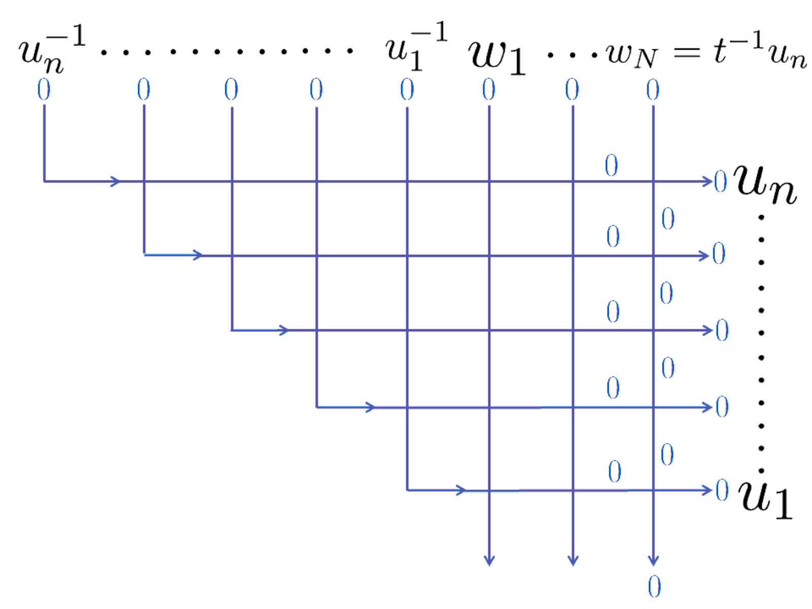
Figure 8: The factorization of WN,n,m(u1,…,un|w1,…,wN|x1,…,xm)W_{N,n,m}(u_{1},\dots,u_{n}|w_{1},\dots,w_{N}|x_{1},\dots,x_{m}), xm≠Nx_{m}\neq N (4.2) .
Refer to caption
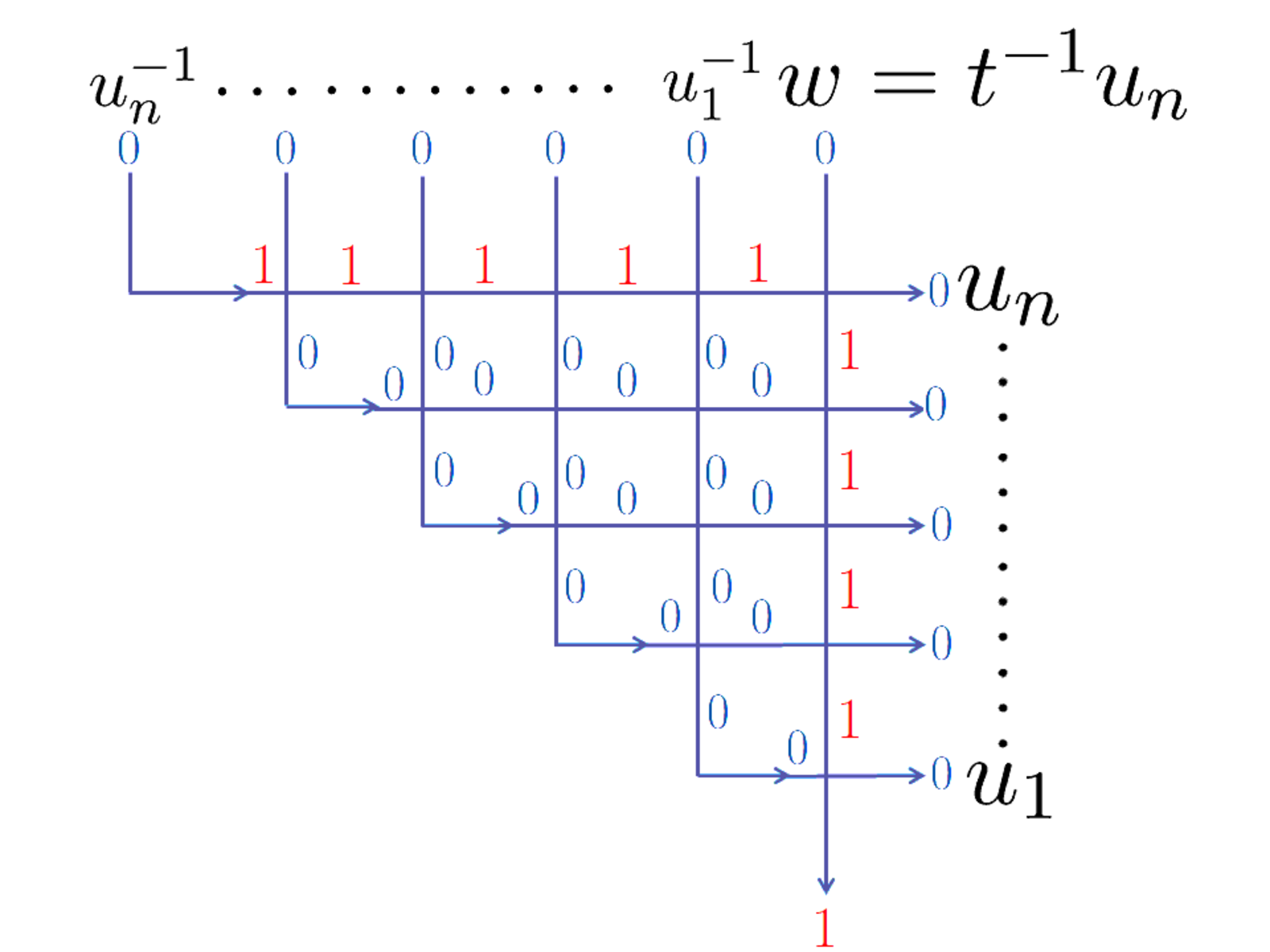
Figure 9: The recursion relation WN,n,m(u1,…,un|w1,…,wN|x1,…,xm)W_{N,n,m}(u_{1},\dots,u_{n}|w_{1},\dots,w_{N}|x_{1},\dots,x_{m}) evaluated at w=t−1​unw=t^{-1}u_{n} for the case N=m=1N=m=1, x1=1x_{1}=1 (4.3).
Refer to caption
Figure 10: The factorization of WN,n,m(u1,…,un|w1,…,wN|x1,…,xm)W_{N,n,m}(u_{1},\dots,u_{n}|w_{1},\dots,w_{N}|x_{1},\dots,x_{m}) for the case N=1,m=0N=1,\ m=0 (4.4).

4 Izergin-Korepin analysis

In this section, we list and prove the properties of the wavefunctions
WN,n,m(u1,…,un|w1,…,wN|x1,…,xm)W_{N,n,m}(u_{1},\dots,u_{n}|w_{1},\dots,w_{N}|x_{1},\dots,x_{m}) defined in the last section by extending the Izergin-Korepin analysis [5, 6, 48] on the domain wall boundary partition function with triangular boundary in our recent paper [44].

Proposition 4.1.

The wavefunctions WN,n,m(u1,…,un|w1,…,wN|x1,…,xm)W_{N,n,m}(u_{1},\dots,u_{n}|w_{1},\dots,w_{N}|x_{1},\dots,x_{m}) satisfies the following properties.

(1) WN,n,m(u1,…,un|w1,…,wN|x1,…,xm)W_{N,n,m}(u_{1},\dots,u_{n}|w_{1},\dots,w_{N}|x_{1},\dots,x_{m}) is a polynomial of degree n−1n-1 in wNw_{N} if xm=Nx_{m}=N and degree nn if xm≠Nx_{m}\neq N.
(2) WN,n,m(u1,…,un|w1,…,wN|x1,…,xm)W_{N,n,m}(u_{1},\dots,u_{n}|w_{1},\dots,w_{N}|x_{1},\dots,x_{m}) is symmetric with respect to uju_{j}, j=1,…,nj=1,\dots,n.
(3) The following recursive relations between the wavefunctions hold if xm=Nx_{m}=N (Figure 7):

WN,n,m(u1,…,un|w1,…,wN|x1,…,xm)|wN=t−1​un\displaystyle W_{N,n,m}(u_{1},\dots,u_{n}|w_{1},\dots,w_{N}|x_{1},\dots,x_{m})|_{w_{N}=t^{-1}u_{n}}
=\displaystyle= (1−t)​∏j=1n−1(t​uj−un)​∏j=1n(uj​un−1)​∏j=1N−1(un−wj)\displaystyle(1-t)\prod_{j=1}^{n-1}(tu_{j}-u_{n})\prod_{j=1}^{n}(u_{j}u_{n}-1)\prod_{j=1}^{N-1}(u_{n}-w_{j})
×WN−1,n−1,m−1(u1,…,un−1|w1,…,wN−1|x1,…,xm−1).\displaystyle\times W_{N-1,n-1,m-1}(u_{1},\dots,u_{n-1}|w_{1},\dots,w_{N-1}|x_{1},\dots,x_{m-1}). (4.1)

If xm≠Nx_{m}\neq N, the following factorizations hold for the wavefunctions (Figure 8):

WN,n,m(u1,…,un|w1,…,wN|x1,…,xm)\displaystyle W_{N,n,m}(u_{1},\dots,u_{n}|w_{1},\dots,w_{N}|x_{1},\dots,x_{m})
=\displaystyle= ∏j=1n(uj−twN)WN−1,n,m(u1,…,un|w1,…,wN−1|x1,…,xm).\displaystyle\prod_{j=1}^{n}(u_{j}-tw_{N})W_{N-1,n,m}(u_{1},\dots,u_{n}|w_{1},\dots,w_{N-1}|x_{1},\dots,x_{m}). (4.2)

(4) The following explicit evaluations hold for the case N=m=1N=m=1 (Figure 9):

W1,n,1​(u1,…,un​|w|​1)|w=t−1​un\displaystyle W_{1,n,1}(u_{1},\dots,u_{n}|w|1)|_{w=t^{-1}u_{n}}
=\displaystyle= (1−t)​∏j=1n−1(t​uj−un)​(B​uj−A)​∏j=1n(uj​un−1)​∏1≤j<k≤n−1(uj​uk−t).\displaystyle(1-t)\prod_{j=1}^{n-1}(tu_{j}-u_{n})(Bu_{j}-A)\prod_{j=1}^{n}(u_{j}u_{n}-1)\prod_{1\leq j<k\leq n-1}(u_{j}u_{k}-t). (4.3)

If N=1,m=0N=1,\ m=0, the following explicit evaluation holds (Figure 10):

W1,n,0​(u1,…,un|w)=∏j=1n(B​uj−A)​∏j=1n(uj−t​w)​∏1≤j<k≤n(uj​uk−t).\displaystyle W_{1,n,0}(u_{1},\dots,u_{n}|w)=\prod_{j=1}^{n}(Bu_{j}-A)\prod_{j=1}^{n}(u_{j}-tw)\prod_{1\leq j<k\leq n}(u_{j}u_{k}-t). (4.4)
Proof.

Property (1) for the case xm=Nx_{m}=N can be easily shown in the same way with the domain wall boundary partition function (with triangular boundary) by inserting the completeness relation in one spin down state sector.

For the case xm≠Nx_{m}\neq N, one can also easily show by its graphical representation and the ice rule of the RR-matrix ⟨γ|⟨δ|Ra​b(u,w)|α⟩ab|β⟩ba=0{}_{a}\langle\gamma|{}_{b}\langle\delta|R_{ab}(u,w)|\alpha\rangle_{a}|\beta\rangle_{b}=0 unless α+β=γ+δ\alpha+\beta=\gamma+\delta. Using the ice rule, one finds that the RR-matrices on the rightmost row freeze (Figure 8). The contribution to the weights from the freezed rightmost row is ∏j=1n(uj−t​wN)\prod_{j=1}^{n}(u_{j}-tw_{N}), and the remaining part is nothing but the wavefunctions WN−1,n,m(u1,…,un|w1,…,wN−1|x1,…,xm)W_{N-1,n,m}(u_{1},\dots,u_{n}|w_{1},\dots,w_{N-1}|x_{1},\dots,x_{m}). This shows that WN,n,m(u1,…,un|w1,…,wN|x1,…,xm)W_{N,n,m}(u_{1},\dots,u_{n}|w_{1},\dots,w_{N}|x_{1},\dots,x_{m}) has the following factorization for the case xm≠Nx_{m}\neq N

WN,n,m(u1,…,un|w1,…,wN|x1,…,xm)\displaystyle W_{N,n,m}(u_{1},\dots,u_{n}|w_{1},\dots,w_{N}|x_{1},\dots,x_{m})
=\displaystyle= ∏j=1n(uj−twN)WN−1,n,m(u1,…,un|w1,…,wN−1|x1,…,xm),\displaystyle\prod_{j=1}^{n}(u_{j}-tw_{N})W_{N-1,n,m}(u_{1},\dots,u_{n}|w_{1},\dots,w_{N-1}|x_{1},\dots,x_{m}), (4.5)

which is nothing but (4.2). This relation shows Properties (1) and (3) for the case xm≠Nx_{m}\neq N.

Property (2) can be shown by the standard railroad argument using the Yang-Baxter relation and the reflection equation repeatedly, exactly in the same way we proved for the case of the domain wall boundary partition function [44]. We remark that the wavefunctions WN,n,m(u1,…,un|w1,…,wN|x1,…,xm)W_{N,n,m}(u_{1},\dots,u_{n}|w_{1},\dots,w_{N}|x_{1},\dots,x_{m}) is no more symmetric with respect to wjw_{j}, j=1,…,mj=1,\dots,m in general unlike the domain wall boundary partition function. This comes from the fact that the dual spin state ⟨x1⋯xm|\langle x_{1}\cdots x_{m}| which is used to construct the wavefunctions is not a consecutive sequence of down spins anymore in general. Note that the dual spin state ⟨x1⋯xm|\langle x_{1}\cdots x_{m}| does not have any influence on the railroad argument to prove the commutativity of the spectral parameters {u}n\{u\}_{n}.

Property (3) for the case xm=Nx_{m}=N can be proved with the help of the graphical representation of the wavefunctions WN,n,m(u1,…,un|w1,…,wN|x1,…,xm)W_{N,n,m}(u_{1},\dots,u_{n}|w_{1},\dots,w_{N}|x_{1},\dots,x_{m}), and can be showed essentially in the same way with proving a similiar property for the domain wall boundary partition function Zn,m​({u}n|{w}m)Z_{n,m}(\{u\}_{n}|\{w\}_{m}) [44]. To show (4.1), let us see what happens when one sets wNw_{N} as wN=t−1​unw_{N}=t^{-1}u_{n} (see Figure 7). One first sees that the RR-matrix at the top right corner freezes due to the vanishing property ⟨0|⟨0|R(un,wN=t−1un)|0⟩−nN|0⟩N−n=0{}_{-n}\langle 0|{}_{N}\langle 0|R(u_{n},w_{N}=t^{-1}u_{n})|0\rangle_{-n}|0\rangle_{N}=0. Then using the ice rule of the RR-matrix, one finds the top row and the rightmost column freeze. The total contribution of the weights from the freezed part can be calculated by multiplying all the matrix elements of the RR-matrix and the KK-matrix which appear, and we find it is given by (1−t)​∏j=1n−1(t​uj−un)​∏j=1n(uj​un−1)​∏j=1N−1(un−wj)(1-t)\prod_{j=1}^{n-1}(tu_{j}-u_{n})\prod_{j=1}^{n}(u_{j}u_{n}-1)\prod_{j=1}^{N-1}(u_{n}-w_{j}). Next, one finds that the remaining unfreezed part is nothing but the wavefunctions WN−1,n−1,m−1(u1,…,un−1|w1,…,wN−1|x1,…,xm−1)W_{N-1,n-1,m-1}(u_{1},\dots,u_{n-1}|w_{1},\dots,w_{N-1}|x_{1},\dots,x_{m-1}) , from which one concludes that WN,n,m(u1,…,un|w1,…,wN|x1,…,xm)W_{N,n,m}(u_{1},\dots,u_{n}|w_{1},\dots,w_{N}|x_{1},\dots,x_{m}) evaluated at wN=t−1​unw_{N}=t^{-1}u_{n} is the product of (1−t)​∏j=1n−1(t​uj−un)​∏j=1n(uj​un−1)​∏j=1N−1(un−wj)(1-t)\prod_{j=1}^{n-1}(tu_{j}-u_{n})\prod_{j=1}^{n}(u_{j}u_{n}-1)\prod_{j=1}^{N-1}(u_{n}-w_{j}) and
WN−1,n−1,m−1(u1,…,un−1|w1,…,wN−1|x1,…,xm−1)W_{N-1,n-1,m-1}(u_{1},\dots,u_{n-1}|w_{1},\dots,w_{N-1}|x_{1},\dots,x_{m-1}). This shows (4.1).

What remains to be shown is Property (4), which can be regarded as the initial condition of the recursion relation (Property (3)).

Property (4) for the case m=1m=1 is shown in [44]. We include the proof here for the sake of completeness. This can be shown in the same way as Property (3). Let us denote w1w_{1} as ww for simplicity. From its graphical representation, one finds great simplication occurs for the wavefunction W1,n,1​(u1,…,un​|w|​1)W_{1,n,1}(u_{1},\dots,u_{n}|w|1) (Figure 9). When one sets w=t−1​unw=t^{-1}u_{n}, one first finds that the top row and the rightmost column freeze. We make a further observation on W1,n,1​(u1,…,un​|w|​1)W_{1,n,1}(u_{1},\dots,u_{n}|w|1). Using the property ⟨0|Ka(u)|1⟩aa=0{}_{a}\langle 0|K_{a}(u)|1\rangle_{a}=0 of the triangular KK-matrix (2), one finds that all spins on the bottom row freeze, and this freezing process continues and we finally find that all spins get freezed. Multiplying all the appearing matrix elements of the RR-matrix and the KK-matrix, one finds the total contribution is given by (1−t)​∏j=1n−1(t​uj−un)​(B​uj−A)​∏j=1n(uj​un−1)​∏1≤j<k≤n−1(uj​uk−t)(1-t)\prod_{j=1}^{n-1}(tu_{j}-u_{n})(Bu_{j}-A)\prod_{j=1}^{n}(u_{j}u_{n}-1)\prod_{1\leq j<k\leq n-1}(u_{j}u_{k}-t), hence (4.3) is shown.

Property (4) for the case m=0m=0 can also be proved in the same way. By drawing the graphical representation of W1,n,0​(u1,…,un|w)W_{1,n,0}(u_{1},\dots,u_{n}|w), one finds by using the ice rule of the RR-matrix and the property ⟨0|Ka(u)|1⟩aa=0{}_{a}\langle 0|K_{a}(u)|1\rangle_{a}=0 of the KK-matrix that all spins get freezed. Multiplying all the appearing matrix elements of the RR-matrix and the KK-matrix, one finds the total contribution to the wavefunctions is given by ∏j=1n(B​uj−A)​∏j=1n(uj−t​w)​∏1≤j<k≤n(uj​uk−t)\prod_{j=1}^{n}(Bu_{j}-A)\prod_{j=1}^{n}(u_{j}-tw)\prod_{1\leq j<k\leq n}(u_{j}u_{k}-t), from which one concludes (4.4) holds. See Figure 10 for the graphical representation of W1,n,0​(u1,…,un|w)W_{1,n,0}(u_{1},\dots,u_{n}|w).

∎

5 Symmetric functions

In this section, we introduce a class of symmetric function, and prove that the symmetric function represents the wavefunctions of the six-vertex model with triangular boundary WN,n,m(u1,…,un|w1,…,wN|x1,…,xm)W_{N,n,m}(u_{1},\dots,u_{n}|w_{1},\dots,w_{N}|x_{1},\dots,x_{m}) by showing that it satisfies all the required properties derived by the Izergin-Korepin analysis in the last section.

Definition 5.1.

We define the following symmetric function
FN,n,m(u1,…,un|w1,…,wN|x1,…,xm)F_{N,n,m}(u_{1},\dots,u_{n}|w_{1},\dots,w_{N}|x_{1},\dots,x_{m}) which depends on the symmetric variables u1,…,unu_{1},\dots,u_{n}, complex parameters w1,…,wNw_{1},\dots,w_{N} and integers x1,…,xmx_{1},\dots,x_{m} satisfying 1≤x1<⋯<xm≤N1\leq x_{1}<\cdots<x_{m}\leq N,

FN,n,m(u1,…,un|w1,…,wN|x1,…,xm)\displaystyle F_{N,n,m}(u_{1},\dots,u_{n}|w_{1},\dots,w_{N}|x_{1},\dots,x_{m})
=\displaystyle= 1(n−m)!​∑σ∈Sn∏j=1m∏k=xj+1N(uσ⁡(j)−t​wk)​∏1≤j<k≤mt​uσ⁡(j)−uσ⁡(k)uσ⁡(j)−uσ⁡(k)​(uσ⁡(j)​uσ⁡(k)−1)\displaystyle\frac{1}{(n-m)!}\sum_{\sigma\in S_{n}}\prod_{j=1}^{m}\prod_{k=x_{j}+1}^{N}(u_{\sigma(j)}-tw_{k})\prod_{1\leq j<k\leq m}\frac{tu_{\sigma(j)}-u_{\sigma(k)}}{u_{\sigma(j)}-u_{\sigma(k)}}(u_{\sigma(j)}u_{\sigma(k)}-1)
×∏m+1≤j≤n1≤k≤N(uσ⁡(j)−t​wk)​∏m+1≤j≤n1≤k≤mt​uσ⁡(j)−uσ⁡(k)uσ⁡(j)−uσ⁡(k)​(uσ⁡(j)​uσ⁡(k)−1)\displaystyle\times\prod_{\begin{subarray}{c}m+1\leq j\leq n\\ 1\leq k\leq N\end{subarray}}(u_{\sigma(j)}-tw_{k})\prod_{\begin{subarray}{c}m+1\leq j\leq n\\ 1\leq k\leq m\end{subarray}}\frac{tu_{\sigma(j)}-u_{\sigma(k)}}{u_{\sigma(j)}-u_{\sigma(k)}}(u_{\sigma(j)}u_{\sigma(k)}-1)
×∏j=1m∏k=1xj−1(uσ⁡(j)−wk)​∏m+1≤j<k≤n(uσ⁡(j)​uσ⁡(k)−t)\displaystyle\times\prod_{j=1}^{m}\prod_{k=1}^{x_{j}-1}(u_{\sigma(j)}-w_{k})\prod_{m+1\leq j<k\leq n}(u_{\sigma(j)}u_{\sigma(k)}-t)
×∏j=1m(1−t)​(uσ⁡(j)2−1)​∏j=m+1n(B​uσ⁡(j)−A).\displaystyle\times\prod_{j=1}^{m}(1-t)(u_{\sigma(j)}^{2}-1)\prod_{j=m+1}^{n}(Bu_{\sigma(j)}-A). (5.1)
Theorem 5.2.

The wavefunctions of the six-vertex model with triangular boundary
ZN,n,m(u1,…,un|w1,…,wN|x1,…,xm)Z_{N,n,m}(u_{1},\dots,u_{n}|w_{1},\dots,w_{N}|x_{1},\dots,x_{m}) is explicitly expressed as the symmetric function FN,n,m(u1,…,un|w1,…,wN|x1,…,xm)F_{N,n,m}(u_{1},\dots,u_{n}|w_{1},\dots,w_{N}|x_{1},\dots,x_{m})

ZN,n,m(u1,…,un|w1,…,wN|x1,…,xm)=FN,n,m(u1,…,un|w1,…,wN|x1,…,xm).\displaystyle Z_{N,n,m}(u_{1},\dots,u_{n}|w_{1},\dots,w_{N}|x_{1},\dots,x_{m})=F_{N,n,m}(u_{1},\dots,u_{n}|w_{1},\dots,w_{N}|x_{1},\dots,x_{m}). (5.2)
Proof.

We prove this theorem by showing that the symmetric funcion (5.1)
FN,n,m(u1,…,un|w1,…,wN|x1,…,xm)F_{N,n,m}(u_{1},\dots,u_{n}|w_{1},\dots,w_{N}|x_{1},\dots,x_{m}) satisfies all the four Properties in Proposition 4.1.

Let us first show Property (1). First, note that the factor ∏j=1m∏k=xj+1N(uσ⁡(j)−t​wk)\displaystyle\prod_{j=1}^{m}\prod_{k=x_{j}+1}^{N}(u_{\sigma(j)}-tw_{k}) in FN,n,m(u1,…,un|w1,…,wN|x1,…,xm)F_{N,n,m}(u_{1},\dots,u_{n}|w_{1},\dots,w_{N}|x_{1},\dots,x_{m}) is a polynomial of degree m−1m-1 in wNw_{N} if xm=Nx_{m}=N and degree mm if xm≠Nx_{m}\neq N. There is also a factor ∏m+1≤j≤n(uσ⁡(j)−t​wN)\displaystyle\prod_{m+1\leq j\leq n}(u_{\sigma(j)}-tw_{N}) in (5.1) which contributes to the degree of wNw_{N}, and one finds that FN,n,m(u1,…,un|w1,…,wN|x1,…,xm)F_{N,n,m}(u_{1},\dots,u_{n}|w_{1},\dots,w_{N}|x_{1},\dots,x_{m}) is a polynomial of degree n−1n-1 in wNw_{N} if xm=Nx_{m}=N and degree nn if xm≠Nx_{m}\neq N.

It is also easy to find that FN,n,m(u1,…,un|w1,…,wN|x1,…,xm)F_{N,n,m}(u_{1},\dots,u_{n}|w_{1},\dots,w_{N}|x_{1},\dots,x_{m}) is symmetric with respect to uju_{j}, j=1,…,nj=1,\dots,n, since the sum is over all permutations of the variables uju_{j}, j=1,…,nj=1,\dots,n.

Let us show Property (3). We first show the function FN,n,m({u}n|w1,…,wN|x1,…,xm)F_{N,n,m}(\{u\}_{n}|w_{1},\dots,w_{N}|x_{1},\dots,x_{m}) satisfies (4.1) which we have to prove for the case xm=Nx_{m}=N. In this case, first note that the factor

∏j=1m∏k=xj+1N(uσ⁡(j)−t​wk)​∏m+1≤j≤n1≤k≤N(uσ⁡(j)−t​wk),\displaystyle\prod_{j=1}^{m}\prod_{k=x_{j}+1}^{N}(u_{\sigma(j)}-tw_{k})\prod_{\begin{subarray}{c}m+1\leq j\leq n\\ 1\leq k\leq N\end{subarray}}(u_{\sigma(j)}-tw_{k}), (5.3)

in each summand essentially becomes

∏j=1m−1∏k=xj+1N(uσ⁡(j)−t​wk)​∏m+1≤j≤n1≤k≤N(uσ⁡(j)−t​wk).\displaystyle\prod_{j=1}^{m-1}\prod_{k=x_{j}+1}^{N}(u_{\sigma(j)}-tw_{k})\prod_{\begin{subarray}{c}m+1\leq j\leq n\\ 1\leq k\leq N\end{subarray}}(u_{\sigma(j)}-tw_{k}). (5.4)

Then one can extract a factor ∏j=1m−1(uσ⁡(j)−t​wN)​∏j=m+1N(uσ⁡(j)−t​wN)\displaystyle\prod_{j=1}^{m-1}(u_{\sigma(j)}-tw_{N})\prod_{j=m+1}^{N}(u_{\sigma(j)}-tw_{N}) from (5.4). Let us concentrate on this factor. If one substitutes wN=t−1​unw_{N}=t^{-1}u_{n}, this factor vanishes unless σ\sigma satisfies σ⁡(m)=n\sigma(m)=n.

Therefore, only the summands satisfying σ⁡(m)=n\sigma(m)=n in (5.1) survive after the substitution wN=t−1​unw_{N}=t^{-1}u_{n}. Keeping this in mind, one rewrites FN,n,m({u}n|w1,…,wN|x1,…,xm)|wN=t−1​unF_{N,n,m}(\{u\}_{n}|w_{1},\dots,w_{N}|x_{1},\dots,x_{m})|_{w_{N}=t^{-1}u_{n}} by using the symmetric group Sn−1S_{n-1} where every σ′∈Sn−1\sigma^{\prime}\in S_{n-1} satisfies {σ′​(1),⋯,σ′​(m−1),σ′​(m+1),⋯,σ′​(n)}={1,⋯,n−1}\{\sigma^{\prime}(1),\cdots,\sigma^{\prime}(m-1),\sigma^{\prime}(m+1),\cdots,\sigma^{\prime}(n)\}=\{1,\cdots,n-1\} as follows:

FN,n,m(u1,…,un|w1,…,wN|x1,…,xm)|wN=t−1​un\displaystyle F_{N,n,m}(u_{1},\dots,u_{n}|w_{1},\dots,w_{N}|x_{1},\dots,x_{m})|_{w_{N}=t^{-1}u_{n}}
=\displaystyle= 1(n−m)!​∑σ′∈Sn−1∏j=1m−1∏k=xj+1N−1(uσ′​(j)−t​wk)​∏1≤j<k≤m−1t​uσ′​(j)−uσ′​(k)uσ′​(j)−uσ′​(k)​(uσ′​(j)​uσ′​(k)−1)\displaystyle\frac{1}{(n-m)!}\sum_{\sigma^{\prime}\in S_{n-1}}\prod_{j=1}^{m-1}\prod_{k=x_{j}+1}^{N-1}(u_{\sigma^{\prime}(j)}-tw_{k})\prod_{1\leq j<k\leq m-1}\frac{tu_{\sigma^{\prime}(j)}-u_{\sigma^{\prime}(k)}}{u_{\sigma^{\prime}(j)}-u_{\sigma^{\prime}(k)}}(u_{\sigma^{\prime}(j)}u_{\sigma^{\prime}(k)}-1)
×∏m+1≤j≤n1≤k≤N−1(uσ′​(j)−t​wk)​∏m+1≤j≤n1≤k≤m−1t​uσ′​(j)−uσ′​(k)uσ′​(j)−uσ′​(k)​(uσ′​(j)​uσ′​(k)−1)\displaystyle\times\prod_{\begin{subarray}{c}m+1\leq j\leq n\\ 1\leq k\leq N-1\end{subarray}}(u_{\sigma^{\prime}(j)}-tw_{k})\prod_{\begin{subarray}{c}m+1\leq j\leq n\\ 1\leq k\leq m-1\end{subarray}}\frac{tu_{\sigma^{\prime}(j)}-u_{\sigma^{\prime}(k)}}{u_{\sigma^{\prime}(j)}-u_{\sigma^{\prime}(k)}}(u_{\sigma^{\prime}(j)}u_{\sigma^{\prime}(k)}-1)
×∏j=1m−1(t​uσ′​(j)−un)​(uσ′​(j)​un−1)​∏j=m+1n(t​uσ′​(j)−un)​(uσ′​(j)​un−1)\displaystyle\times\prod_{j=1}^{m-1}(tu_{\sigma^{\prime}(j)}-u_{n})(u_{\sigma^{\prime}(j)}u_{n}-1)\prod_{j=m+1}^{n}(tu_{\sigma^{\prime}(j)}-u_{n})(u_{\sigma^{\prime}(j)}u_{n}-1)
×∏j=1m−1∏k=1xj−1(uσ′​(j)−wk)​∏k=1N−1(un−wk)​∏m+1≤j<k≤n(uσ′​(j)​uσ′​(k)−t)\displaystyle\times\prod_{j=1}^{m-1}\prod_{k=1}^{x_{j}-1}(u_{\sigma^{\prime}(j)}-w_{k})\prod_{k=1}^{N-1}(u_{n}-w_{k})\prod_{m+1\leq j<k\leq n}(u_{\sigma^{\prime}(j)}u_{\sigma^{\prime}(k)}-t)
×(1−t)​(un2−1)​∏j=1m−1(1−t)​(uσ′​(j)2−1)​∏j=m+1n(B​uσ′​(j)−A).\displaystyle\times(1-t)(u_{n}^{2}-1)\prod_{j=1}^{m-1}(1-t)(u_{\sigma^{\prime}(j)}^{2}-1)\prod_{j=m+1}^{n}(Bu_{\sigma^{\prime}(j)}-A). (5.5)

One easily notes that the factors ∏k=1N−1(un−wk)\displaystyle\prod_{k=1}^{N-1}(u_{n}-w_{k}) and (1−t)​(un2−1)(1-t)(u_{n}^{2}-1) in the sum are independent of the permutation Sn−1′S^{\prime}_{n-1}. One also finds the factor ∏j=1m−1(t​uσ′​(j)−un)​(uσ′​(j)​un−1)​∏j=m+1n(t​uσ′​(j)−un)​(uσ′​(j)​un−1)\displaystyle\prod_{j=1}^{m-1}(tu_{\sigma^{\prime}(j)}-u_{n})(u_{\sigma^{\prime}(j)}u_{n}-1)\prod_{j=m+1}^{n}(tu_{\sigma^{\prime}(j)}-u_{n})(u_{\sigma^{\prime}(j)}u_{n}-1) is also independent of Sn−1′S^{\prime}_{n-1} since we have

∏j=1m−1(t​uσ′​(j)−un)​(uσ′​(j)​un−1)​∏j=m+1n(t​uσ′​(j)−un)​(uσ′​(j)​un−1)\displaystyle\prod_{j=1}^{m-1}(tu_{\sigma^{\prime}(j)}-u_{n})(u_{\sigma^{\prime}(j)}u_{n}-1)\prod_{j=m+1}^{n}(tu_{\sigma^{\prime}(j)}-u_{n})(u_{\sigma^{\prime}(j)}u_{n}-1)
=\displaystyle= ∏j=1n−1(t​uj−un)​(uj​un−1).\displaystyle\prod_{j=1}^{n-1}(tu_{j}-u_{n})(u_{j}u_{n}-1). (5.6)

Thus, (5.5) can be rewritten furthermore as

FN,n,m(u1,…,un|w1,…,wN|x1,…,xm)|wN=t−1​un\displaystyle F_{N,n,m}(u_{1},\dots,u_{n}|w_{1},\dots,w_{N}|x_{1},\dots,x_{m})|_{w_{N}=t^{-1}u_{n}}
=\displaystyle= (1−t)​(un2−1)​∏j=1n−1(t​uj−un)​(uj​un−1)​∏k=1N−1(un−wk)\displaystyle(1-t)(u_{n}^{2}-1)\prod_{j=1}^{n-1}(tu_{j}-u_{n})(u_{j}u_{n}-1)\prod_{k=1}^{N-1}(u_{n}-w_{k})
×1(n−m)!​∑σ′∈Sn−1∏j=1m−1∏k=xj+1N−1(uσ′​(j)−t​wk)​∏1≤j<k≤m−1t​uσ′​(j)−uσ′​(k)uσ′​(j)−uσ′​(k)​(uσ′​(j)​uσ′​(k)−1)\displaystyle\times\frac{1}{(n-m)!}\sum_{\sigma^{\prime}\in S_{n-1}}\prod_{j=1}^{m-1}\prod_{k=x_{j}+1}^{N-1}(u_{\sigma^{\prime}(j)}-tw_{k})\prod_{1\leq j<k\leq m-1}\frac{tu_{\sigma^{\prime}(j)}-u_{\sigma^{\prime}(k)}}{u_{\sigma^{\prime}(j)}-u_{\sigma^{\prime}(k)}}(u_{\sigma^{\prime}(j)}u_{\sigma^{\prime}(k)}-1)
×∏m+1≤j≤n1≤k≤N−1(uσ′​(j)−t​wk)​∏m+1≤j≤n1≤k≤m−1t​uσ′​(j)−uσ′​(k)uσ′​(j)−uσ′​(k)​(uσ′​(j)​uσ′​(k)−1)\displaystyle\times\prod_{\begin{subarray}{c}m+1\leq j\leq n\\ 1\leq k\leq N-1\end{subarray}}(u_{\sigma^{\prime}(j)}-tw_{k})\prod_{\begin{subarray}{c}m+1\leq j\leq n\\ 1\leq k\leq m-1\end{subarray}}\frac{tu_{\sigma^{\prime}(j)}-u_{\sigma^{\prime}(k)}}{u_{\sigma^{\prime}(j)}-u_{\sigma^{\prime}(k)}}(u_{\sigma^{\prime}(j)}u_{\sigma^{\prime}(k)}-1)
×∏j=1m−1∏k=1xj−1(uσ′​(j)−wk)​∏m+1≤j<k≤n(uσ′​(j)​uσ′​(k)−t)\displaystyle\times\prod_{j=1}^{m-1}\prod_{k=1}^{x_{j}-1}(u_{\sigma^{\prime}(j)}-w_{k})\prod_{m+1\leq j<k\leq n}(u_{\sigma^{\prime}(j)}u_{\sigma^{\prime}(k)}-t)
×∏j=1m−1(1−t)​(uσ′​(j)2−1)​∏j=m+1n(B​uσ′​(j)−A).\displaystyle\times\prod_{j=1}^{m-1}(1-t)(u_{\sigma^{\prime}(j)}^{2}-1)\prod_{j=m+1}^{n}(Bu_{\sigma^{\prime}(j)}-A). (5.7)

Noting

1(n−m)!​∑σ′∈Sn−1∏j=1m−1∏k=xj+1N−1(uσ′​(j)−t​wk)​∏1≤j<k≤m−1t​uσ′​(j)−uσ′​(k)uσ′​(j)−uσ′​(k)​(uσ′​(j)​uσ′​(k)−1)\displaystyle\frac{1}{(n-m)!}\sum_{\sigma^{\prime}\in S_{n-1}}\prod_{j=1}^{m-1}\prod_{k=x_{j}+1}^{N-1}(u_{\sigma^{\prime}(j)}-tw_{k})\prod_{1\leq j<k\leq m-1}\frac{tu_{\sigma^{\prime}(j)}-u_{\sigma^{\prime}(k)}}{u_{\sigma^{\prime}(j)}-u_{\sigma^{\prime}(k)}}(u_{\sigma^{\prime}(j)}u_{\sigma^{\prime}(k)}-1)
×∏m+1≤j≤n1≤k≤N−1(uσ′​(j)−t​wk)​∏m+1≤j≤n1≤k≤m−1t​uσ′​(j)−uσ′​(k)uσ′​(j)−uσ′​(k)​(uσ′​(j)​uσ′​(k)−1)\displaystyle\times\prod_{\begin{subarray}{c}m+1\leq j\leq n\\ 1\leq k\leq N-1\end{subarray}}(u_{\sigma^{\prime}(j)}-tw_{k})\prod_{\begin{subarray}{c}m+1\leq j\leq n\\ 1\leq k\leq m-1\end{subarray}}\frac{tu_{\sigma^{\prime}(j)}-u_{\sigma^{\prime}(k)}}{u_{\sigma^{\prime}(j)}-u_{\sigma^{\prime}(k)}}(u_{\sigma^{\prime}(j)}u_{\sigma^{\prime}(k)}-1)
×∏j=1m−1∏k=1xj−1(uσ′​(j)−wk)​∏m+1≤j<k≤n(uσ′​(j)​uσ′​(k)−t)\displaystyle\times\prod_{j=1}^{m-1}\prod_{k=1}^{x_{j}-1}(u_{\sigma^{\prime}(j)}-w_{k})\prod_{m+1\leq j<k\leq n}(u_{\sigma^{\prime}(j)}u_{\sigma^{\prime}(k)}-t)
×∏j=1m−1(1−t)​(uσ′​(j)2−1)​∏j=m+1n(B​uσ′​(j)−A)\displaystyle\times\prod_{j=1}^{m-1}(1-t)(u_{\sigma^{\prime}(j)}^{2}-1)\prod_{j=m+1}^{n}(Bu_{\sigma^{\prime}(j)}-A)
=\displaystyle= FN−1,n−1,m−1(u1,…,un−1|w1,…,wN−1|x1,…,xm−1),\displaystyle F_{N-1,n-1,m-1}(u_{1},\dots,u_{n-1}|w_{1},\dots,w_{N-1}|x_{1},\dots,x_{m-1}), (5.8)

one finds that (5.7) is nothing but the following recursion relation for the symmetric function FN,n,m(u1,…,un|w1,…,wN|x1,…,xm)F_{N,n,m}(u_{1},\dots,u_{n}|w_{1},\dots,w_{N}|x_{1},\dots,x_{m})

FN,n,m(u1,…,un|w1,…,wN|x1,…,xm)|wN=t−1​un\displaystyle F_{N,n,m}(u_{1},\dots,u_{n}|w_{1},\dots,w_{N}|x_{1},\dots,x_{m})|_{w_{N}=t^{-1}u_{n}}
=\displaystyle= (1−t)​∏j=1n−1(t​uj−un)​∏j=1n(uj​un−1)​∏j=1N−1(un−wj)\displaystyle(1-t)\prod_{j=1}^{n-1}(tu_{j}-u_{n})\prod_{j=1}^{n}(u_{j}u_{n}-1)\prod_{j=1}^{N-1}(u_{n}-w_{j})
×FN−1,n−1,m−1(u1,…,un−1|w1,…,wN−1|x1,…,xm−1),\displaystyle\times F_{N-1,n-1,m-1}(u_{1},\dots,u_{n-1}|w_{1},\dots,w_{N-1}|x_{1},\dots,x_{m-1}), (5.9)

which is exactly the same recursion relation the wavefunctions
WN,n,m(u1,…,un|w1,…,wN|x1,…,xm)W_{N,n,m}(u_{1},\dots,u_{n}|w_{1},\dots,w_{N}|x_{1},\dots,x_{m}) must satisfy. Hence, Property (3) for the case xm=Nx_{m}=N is proved.

The case xm≠Nx_{m}\neq N can be shown in a similar but much simpler way. In this case we can rewrite FN,n,m(u1,…,un|w1,…,wN|x1,…,xm)F_{N,n,m}(u_{1},\dots,u_{n}|w_{1},\dots,w_{N}|x_{1},\dots,x_{m}) as

FN,n,m(u1,…,un|w1,…,wN|x1,…,xm)\displaystyle F_{N,n,m}(u_{1},\dots,u_{n}|w_{1},\dots,w_{N}|x_{1},\dots,x_{m})
=\displaystyle= 1(n−m)!​∑σ∈Sn∏j=1m∏k=xj+1N−1(uσ⁡(j)−t​wk)​∏j=1m(uσ⁡(j)−t​wN)​∏1≤j<k≤mt​uσ⁡(j)−uσ⁡(k)uσ⁡(j)−uσ⁡(k)​(uσ⁡(j)​uσ⁡(k)−1)\displaystyle\frac{1}{(n-m)!}\sum_{\sigma\in S_{n}}\prod_{j=1}^{m}\prod_{k=x_{j}+1}^{N-1}(u_{\sigma(j)}-tw_{k})\prod_{j=1}^{m}(u_{\sigma(j)}-tw_{N})\prod_{1\leq j<k\leq m}\frac{tu_{\sigma(j)}-u_{\sigma(k)}}{u_{\sigma(j)}-u_{\sigma(k)}}(u_{\sigma(j)}u_{\sigma(k)}-1)
×∏m+1≤j≤n1≤k≤N−1(uσ⁡(j)−t​wk)​∏j=m+1n(uσ⁡(j)−t​wN)​∏m+1≤j≤n1≤k≤mt​uσ⁡(j)−uσ⁡(k)uσ⁡(j)−uσ⁡(k)​(uσ⁡(j)​uσ⁡(k)−1)\displaystyle\times\prod_{\begin{subarray}{c}m+1\leq j\leq n\\ 1\leq k\leq N-1\end{subarray}}(u_{\sigma(j)}-tw_{k})\prod_{j=m+1}^{n}(u_{\sigma(j)}-tw_{N})\prod_{\begin{subarray}{c}m+1\leq j\leq n\\ 1\leq k\leq m\end{subarray}}\frac{tu_{\sigma(j)}-u_{\sigma(k)}}{u_{\sigma(j)}-u_{\sigma(k)}}(u_{\sigma(j)}u_{\sigma(k)}-1)
×∏j=1m∏k=1xj−1(uσ⁡(j)−wk)​∏m+1≤j<k≤n(uσ⁡(j)​uσ⁡(k)−t)\displaystyle\times\prod_{j=1}^{m}\prod_{k=1}^{x_{j}-1}(u_{\sigma(j)}-w_{k})\prod_{m+1\leq j<k\leq n}(u_{\sigma(j)}u_{\sigma(k)}-t)
×∏j=1m(1−t)​(uσ⁡(j)2−1)​∏j=m+1n(B​uσ⁡(j)−A).\displaystyle\times\prod_{j=1}^{m}(1-t)(u_{\sigma(j)}^{2}-1)\prod_{j=m+1}^{n}(Bu_{\sigma(j)}-A). (5.10)

The product of the factors ∏j=1m(uσ⁡(j)−t​wN)\displaystyle\prod_{j=1}^{m}(u_{\sigma(j)}-tw_{N}) and ∏j=m+1n(uσ⁡(j)−t​wN)\displaystyle\prod_{j=m+1}^{n}(u_{\sigma(j)}-tw_{N}) becomes

∏j=1m(uσ⁡(j)−t​wN)​∏j=m+1n(uσ⁡(j)−t​wN)=∏j=1n(uj−t​wN),\displaystyle\displaystyle\prod_{j=1}^{m}(u_{\sigma(j)}-tw_{N})\displaystyle\prod_{j=m+1}^{n}(u_{\sigma(j)}-tw_{N})=\prod_{j=1}^{n}(u_{j}-tw_{N}), (5.11)

which becomes independent of the permutation SnS_{n}. Taking this into account, (5.10) can be rewritten as

FN,n,m(u1,…,un|w1,…,wN|x1,…,xm)\displaystyle F_{N,n,m}(u_{1},\dots,u_{n}|w_{1},\dots,w_{N}|x_{1},\dots,x_{m})
=\displaystyle= ∏j=1n(uj−t​wN)​1(n−m)!​∑σ∈Sn∏j=1m∏k=xj+1N−1(uσ⁡(j)−t​wk)​∏1≤j<k≤mt​uσ⁡(j)−uσ⁡(k)uσ⁡(j)−uσ⁡(k)​(uσ⁡(j)​uσ⁡(k)−1)\displaystyle\prod_{j=1}^{n}(u_{j}-tw_{N})\frac{1}{(n-m)!}\sum_{\sigma\in S_{n}}\prod_{j=1}^{m}\prod_{k=x_{j}+1}^{N-1}(u_{\sigma(j)}-tw_{k})\prod_{1\leq j<k\leq m}\frac{tu_{\sigma(j)}-u_{\sigma(k)}}{u_{\sigma(j)}-u_{\sigma(k)}}(u_{\sigma(j)}u_{\sigma(k)}-1)
×∏m+1≤j≤n1≤k≤N−1(uσ⁡(j)−t​wk)​∏m+1≤j≤n1≤k≤mt​uσ⁡(j)−uσ⁡(k)uσ⁡(j)−uσ⁡(k)​(uσ⁡(j)​uσ⁡(k)−1)\displaystyle\times\prod_{\begin{subarray}{c}m+1\leq j\leq n\\ 1\leq k\leq N-1\end{subarray}}(u_{\sigma(j)}-tw_{k})\prod_{\begin{subarray}{c}m+1\leq j\leq n\\ 1\leq k\leq m\end{subarray}}\frac{tu_{\sigma(j)}-u_{\sigma(k)}}{u_{\sigma(j)}-u_{\sigma(k)}}(u_{\sigma(j)}u_{\sigma(k)}-1)
×∏j=1m∏k=1xj−1(uσ⁡(j)−wk)​∏m+1≤j<k≤n(uσ⁡(j)​uσ⁡(k)−t)\displaystyle\times\prod_{j=1}^{m}\prod_{k=1}^{x_{j}-1}(u_{\sigma(j)}-w_{k})\prod_{m+1\leq j<k\leq n}(u_{\sigma(j)}u_{\sigma(k)}-t)
×∏j=1m(1−t)​(uσ⁡(j)2−1)​∏j=m+1n(B​uσ⁡(j)−A)\displaystyle\times\prod_{j=1}^{m}(1-t)(u_{\sigma(j)}^{2}-1)\prod_{j=m+1}^{n}(Bu_{\sigma(j)}-A)
=\displaystyle= ∏j=1n(uj−twN)FN−1,n,m(u1,…,un|w1,…,wN−1|x1,…,xm),\displaystyle\prod_{j=1}^{n}(u_{j}-tw_{N})F_{N-1,n,m}(u_{1},\dots,u_{n}|w_{1},\dots,w_{N-1}|x_{1},\dots,x_{m}), (5.12)

which is also exactly the recursion relation the wavefunctions
WN,n,m(u1,…,un|w1,…,wN|x1,…,xm)W_{N,n,m}(u_{1},\dots,u_{n}|w_{1},\dots,w_{N}|x_{1},\dots,x_{m}) must satisfy for the case xm≠Nx_{m}\neq N.

Let us finally show Property (4). The case m=1m=1 is proved in [44]. We display the proof here for completeness. This can be shown by making further analysis on the symmetric function FN,n,m({u}n|w1,…,wN|x1,…,xm)|wN=t−1​unF_{N,n,m}(\{u\}_{n}|w_{1},\dots,w_{N}|x_{1},\dots,x_{m})|_{w_{N}=t^{-1}u_{n}} for the case N=m=1N=m=1, x1=1x_{1}=1. We first write down the case N=m=1N=m=1, x1=1x_{1}=1 of (5.7) which we used to prove Property (3) (we denote w1w_{1} as ww).

F1,n,1​({u}n​|w|​1)|w=t−1​un=\displaystyle F_{1,n,1}(\{u\}_{n}|w|1)|_{w=t^{-1}u_{n}}= (1−t)​(un2−1)​∏j=1n−1(t​uj−un)​(uj​un−1)\displaystyle(1-t)(u_{n}^{2}-1)\prod_{j=1}^{n-1}(tu_{j}-u_{n})(u_{j}u_{n}-1)
×1(n−1)!​∑σ′∈Sn−1∏2≤j<k≤n(uσ′​(j)​uσ′​(k)−t)​∏j=2n(B​uσ′​(j)−A).\displaystyle\times\frac{1}{(n-1)!}\sum_{\sigma^{\prime}\in S_{n-1}}\prod_{2\leq j<k\leq n}(u_{\sigma^{\prime}(j)}u_{\sigma^{\prime}(k)}-t)\prod_{j=2}^{n}(Bu_{\sigma^{\prime}(j)}-A). (5.13)

Since

∏2≤j<k≤n(uσ′​(j)​uσ′​(k)−t)=\displaystyle\prod_{2\leq j<k\leq n}(u_{\sigma^{\prime}(j)}u_{\sigma^{\prime}(k)}-t)= ∏1≤j<k≤n−1(uj​uk−t),\displaystyle\prod_{1\leq j<k\leq n-1}(u_{j}u_{k}-t), (5.14)
∏j=2n(B​uσ′​(j)−A)=\displaystyle\prod_{j=2}^{n}(Bu_{\sigma^{\prime}(j)}-A)= ∏j=1n−1(B​uj−A),\displaystyle\prod_{j=1}^{n-1}(Bu_{j}-A), (5.15)

the summands are all equal, and the sum in the right hand side of (5.13) becomes (n−1)!​∏1≤j<k≤n−1(uj​uk−t)​∏j=1n−1(B​uj−A)\displaystyle(n-1)!\prod_{1\leq j<k\leq n-1}(u_{j}u_{k}-t)\prod_{j=1}^{n-1}(Bu_{j}-A). Thus, we have the complete factorization

F1,n,1​({u}n​|w|​1)|w=t−1​un\displaystyle F_{1,n,1}(\{u\}_{n}|w|1)|_{w=t^{-1}u_{n}}
=\displaystyle= (1−t)​(un2−1)​∏j=1n−1(t​uj−un)​(uj​un−1)\displaystyle(1-t)(u_{n}^{2}-1)\prod_{j=1}^{n-1}(tu_{j}-u_{n})(u_{j}u_{n}-1)
×1(n−1)!​(n−1)!​∏1≤j<k≤n−1(uj​uk−t)​∏j=1n−1(B​uj−A)\displaystyle\times\frac{1}{(n-1)!}(n-1)!\prod_{1\leq j<k\leq n-1}(u_{j}u_{k}-t)\prod_{j=1}^{n-1}(Bu_{j}-A)
=\displaystyle= (1−t)​∏j=1n−1(t​uj−un)​(B​uj−A)​∏j=1n(uj​un−1)​∏1≤j<k≤n−1(uj​uk−t),\displaystyle(1-t)\prod_{j=1}^{n-1}(tu_{j}-u_{n})(Bu_{j}-A)\prod_{j=1}^{n}(u_{j}u_{n}-1)\prod_{1\leq j<k\leq n-1}(u_{j}u_{k}-t), (5.16)

which implies that F1,n,1​({u}n​|w|​1)F_{1,n,1}(\{u\}_{n}|w|1) satisfies the same property with W1,n,1​({u}n​|w|​1)W_{1,n,1}(\{u\}_{n}|w|1). Hence, Property (4) for the case m=1m=1 is proved.

The case m=0m=0 can be shown in a similar way. Writing down the case N=1,m=0N=1,\ m=0 of (5.7), one immediately sees that all the summands are equal and we have

F1,n,0​({u}n|w)\displaystyle F_{1,n,0}(\{u\}_{n}|w) =1n!​∑σ∈Sn∏j=1n(uσ⁡(j)−t​w)​∏1≤j<k≤n(uσ⁡(j)​uσ⁡(k)−t)​∏j=1n(B​uσ⁡(j)−A)\displaystyle=\frac{1}{n!}\sum_{\sigma\in S_{n}}\prod_{j=1}^{n}(u_{\sigma(j)}-tw)\prod_{1\leq j<k\leq n}(u_{\sigma(j)}u_{\sigma(k)}-t)\prod_{j=1}^{n}(Bu_{\sigma(j)}-A)
=1n!​n!​∏j=1n(uj−t​w)​∏1≤j<k≤n(uj​uk−t)​∏j=1n(B​uj−A)\displaystyle=\frac{1}{n!}n!\prod_{j=1}^{n}(u_{j}-tw)\prod_{1\leq j<k\leq n}(u_{j}u_{k}-t)\prod_{j=1}^{n}(Bu_{j}-A)
=∏j=1n(uj−t​w)​∏1≤j<k≤n(uj​uk−t)​∏j=1n(B​uj−A),\displaystyle=\prod_{j=1}^{n}(u_{j}-tw)\prod_{1\leq j<k\leq n}(u_{j}u_{k}-t)\prod_{j=1}^{n}(Bu_{j}-A), (5.17)

which shows that F1,n,0​({u}n|w)F_{1,n,0}(\{u\}_{n}|w) is the same with W1,n,0​({u}n|w)W_{1,n,0}(\{u\}_{n}|w).

We have proved that the symmetric function FN,n,m(u1,…,un|w1,…,wN|x1,…,xm)F_{N,n,m}(u_{1},\dots,u_{n}|w_{1},\dots,w_{N}|x_{1},\dots,x_{m}) satisfies all the Properties (1), (2), (3) and (4) in Proposition 4.1, hence it is the explicit form of the wavefunctions with triangular boundary ZN,n,m(u1,…,un|w1,…,wN|x1,…,xm)=FN,n,m(u1,…,un|w1,…,wN|x1,…,xm)Z_{N,n,m}(u_{1},\dots,u_{n}|w_{1},\dots,w_{N}|x_{1},\dots,x_{m})=F_{N,n,m}(u_{1},\dots,u_{n}|w_{1},\dots,w_{N}|x_{1},\dots,x_{m}). ∎

6 Conclusion

In this paper, we introduced an analogue of the wavefunctions of an integrable six-vertex model with triangular boundary. We used the Uq​(s​l2)U_{q}(sl_{2}) RR-matrix as the bulk weights and a triangular KK-matrix as the boundary weights. We extended our recent work [44] of the Izergin-Korepin analysis on the domain wall boundary partition function to the wavefunctions and listed the properties about the degree, symmetry, two recursion relations and two initial conditions. We proved that a class of certain explicit symmetric functions satisfies all the required properties, which means that the symmetric functions is nothing but the explicit form which represents the wavefunctions with triangular boundary.

The main motivation for introducing and studying the wavefunctions with triangular boundary is that there are similar combinatorial objects in algebraic combinatorics and Schubert calculus such as the non-intersecting lattice paths and excited Young diagrams [39, 40, 41, 42, 43]. Some of those combinatorial objects can be regarded as the wavefunctions of integrable lattice models with triangular boundary, with the bulk weights given by an RR-matrix of an integrable five-vertex model, and the boundary weights given by a triangular KK-matrix. Our result can be regarded as an extension of these combinatorial objects by using the six-vertex Uq​(s​l2)U_{q}(sl_{2}) RR-matrix as the bulk weights, and more general triangular KK-matrix as the boundary weights. The ordinary wavefunctions [24, 25] is represented by the Grothendieck polynomials of type AA Grassmannian variety and their quantum group deformations. See the Appendix for a proof of the ordinarywavefunctions based on the Izergin-Korepin analysis.

We called the class of partition functions treated in this paper as “the wavefunctions”. For the case of ordinary wavefunctions, it is the inner product between the state vector of spins and the off-shell Bethe vector, which becomes the eigenvector of the XXZ spin chain when the Bethe ansatz equations are imposed on the spectral parameters. However, we do not know at this moment if the “off-shell” Bethe vector for the case of triangular boundary becomes an eigenfunction of some Hamiltonian or transfer matrix. This is the reason why we sometimes called the partition functions treated in this paper as “an analogue of the wavefunctions”. It seems worthwhile to investigate whether such Hamiltonian or transfer matrix exist, and if so, what are their explicit forms.

Extending the analysis to various integrable models such as the higher rank models, elliptic models is also an interesting topic. Formulating the wavefunctions of elliptic integrable models [49] by using the dynamical RR-matrix as the bulk weights and the triangular elliptic KK-matrix [50, 51] as the boundary weights, using the Izergin-Korepin analysis and finding the corresponding elliptic symmetric functions with the help of complex analysis is an interesting work. See [52, 53, 54, 55, 56, 57, 58, 59, 60] for examples on the treatment of the domain wall boundary partition functions and scalar products of the elliptic and trigonometric face models by using various methods developed to analzye those objects. Also interesting topics are to study wavefunctions constructed from the RR- and KK-matrices of higher dimensional representations. See [61] for example on this direction.

Acknowledgements

This work was partially supported by grant-in-Aid for Research Activity start-up No. 15H06218 and Scientific Research (C) No. 16K05468.

Appendix A Ordinary wavefunctions

Refer to caption
Figure 11: The LL-operator L⁡(u,w)L(u,w) (A). The horizontal line is the space WW, and the vertical line is the space VV.

We give here the Izergin-Korepin analysis on the ordinary wavefunctions in this Appendix. We remark that the result presented here can be obtained by applying the general result on the ordinary wavefunctions, for example [29, 30], to the following LL-operator presented below. We present a proof based on the Izergin-Korepin analysis here since it is an illustrative example.

We analyze the wavefunctions constructed from the following generalized LL-operator [26] (Figure 11)

La​j​(u,w,a,b,c,d,e,f)=(a​u+b​w0000a​t​u+b​w(1−t)​c​u00(1−t)​d​we​u+f​w0000e​u+t​f​w),\displaystyle L_{aj}(u,w,a,b,c,d,e,f)=\left(\begin{array}[]{cccc}au+bw&0&0&0\\ 0&atu+bw&(1-t)cu&0\\ 0&(1-t)dw&eu+fw&0\\ 0&0&0&eu+tfw\end{array}\right),

acting on the tensor product Wa⊗VjW_{a}\otimes V_{j} where VjV_{j} is also a complex two-dimensional vector space, and the parameters aa, bb, cc, dd, ee and ff are constant parameters (do not depend on the spectral parameter uu) and must obey the following relations

(1−t)​c​d+a​f−b​e=0,(t2−t)​c​d+t2​a​f−b​e=0.\displaystyle(1-t)cd+af-be=0,\ (t^{2}-t)cd+t^{2}af-be=0. (A.6)

If one assumes t≠1t\neq 1, the relations (A.6) further reduce to

c​d+a​f=0,t​c​d+b​e=0.\displaystyle cd+af=0,\ tcd+be=0. (A.7)

We frequently abbreviate La​j​(u,w,a,b,c,d,e,f)L_{aj}(u,w,a,b,c,d,e,f) as La​j​(u,w)L_{aj}(u,w) for simplicity. The matrix elements of the LL-operator (A) is explicitly given by

⟨0|⟨0|La​j(u,w)|0⟩aj|0⟩ja\displaystyle{}_{a}\langle 0|{}_{j}\langle 0|L_{aj}(u,w)|0\rangle_{a}|0\rangle_{j} =a​u+b​w,\displaystyle=au+bw, (A.8)
⟨0|⟨1|La​j(u,w)|0⟩aj|1⟩ja\displaystyle{}_{a}\langle 0|{}_{j}\langle 1|L_{aj}(u,w)|0\rangle_{a}|1\rangle_{j} =a​t​u+b​w,\displaystyle=atu+bw, (A.9)
⟨0|⟨1|La​j(u,w)|1⟩aj|0⟩ja\displaystyle{}_{a}\langle 0|{}_{j}\langle 1|L_{aj}(u,w)|1\rangle_{a}|0\rangle_{j} =(1−t)​c​u,\displaystyle=(1-t)cu, (A.10)
⟨1|⟨0|La​j(u,w)|0⟩aj|1⟩ja\displaystyle{}_{a}\langle 1|{}_{j}\langle 0|L_{aj}(u,w)|0\rangle_{a}|1\rangle_{j} =(1−t)​d​w,\displaystyle=(1-t)dw, (A.11)
⟨1|⟨0|La​j(u,w)|1⟩aj|0⟩ja\displaystyle{}_{a}\langle 1|{}_{j}\langle 0|L_{aj}(u,w)|1\rangle_{a}|0\rangle_{j} =e​u+f​w,\displaystyle=eu+fw, (A.12)
⟨1|⟨1|La​j(u,w)|1⟩aj|1⟩ja\displaystyle{}_{a}\langle 1|{}_{j}\langle 1|L_{aj}(u,w)|1\rangle_{a}|1\rangle_{j} =e​u+f​t​w.\displaystyle=eu+ftw. (A.13)
Refer to caption
Figure 12: The ordinary wavefunctions OWN,n(u1,…,un|w1,…,wN|x1,…,xn)OW_{N,n}(u_{1},\dots,u_{n}|w_{1},\dots,w_{N}|x_{1},\dots,x_{n}) (A.23). This figure illustrates the case N=8,n=5,x1=1,x2=2,x3=4,x4=6,x5=7N=8,\ n=5,\ x_{1}=1,\ x_{2}=2,\ x_{3}=4,\ x_{4}=6,\ x_{5}=7.
Refer to caption
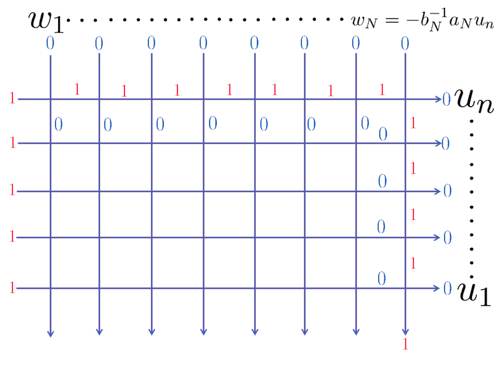
Figure 13: The recursion relation OWN,n(u1,…,un|w1,…,wN|x1,…,xn)OW_{N,n}(u_{1},\dots,u_{n}|w_{1},\dots,w_{N}|x_{1},\dots,x_{n}), xn=Nx_{n}=N evaluated at wN=−bN−1​aN​unw_{N}=-b_{N}^{-1}a_{N}u_{n} (A.24) .
Refer to caption
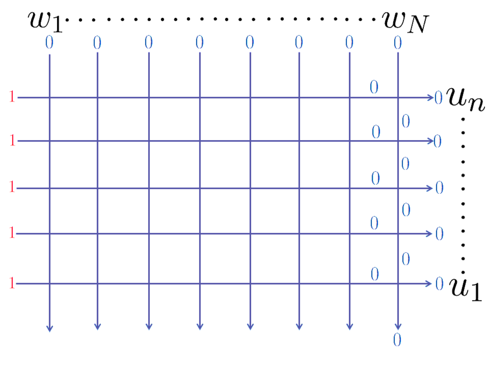
Figure 14: The factorization of OWN,n(u1,…,un|w1,…,wN|x1,…,xn)OW_{N,n}(u_{1},\dots,u_{n}|w_{1},\dots,w_{N}|x_{1},\dots,x_{n}), xn≠Nx_{n}\neq N (A.25) .

The LL-operator (A) together with the Uq​(s​l2)U_{q}(sl_{2}) RR-matrix (2) satisfies the R​L​LRLL-type Yang-Baxter relation

Ra​b​(u1,u2)​La​j​(u1,w)​Lb​j​(u2,w)=Lb​j​(u2,w)​La​j​(u1,w)​Ra​b​(u1,u2),\displaystyle R_{ab}(u_{1},u_{2})L_{aj}(u_{1},w)L_{bj}(u_{2},w)=L_{bj}(u_{2},w)L_{aj}(u_{1},w)R_{ab}(u_{1},u_{2}), (A.14)

acting on Wa⊗Wb⊗VjW_{a}\otimes W_{b}\otimes V_{j}. (A) and (A.14) contains the Uq​(s​l2)U_{q}(sl_{2}) RR-matrix (2) and the R​R​RRRR-type Yang-Baxter relation (2.12) as a special case a=1a=1, b=−tb=-t, c=1c=1, d=1d=1, e=1e=1, f=−1f=-1.

In the quantum inverse scattering method, what we first do is to construct the monodromy matrix Ta​(u|w1,…,wN)T_{a}(u|w_{1},\dots,w_{N}) from the LL-operator as

Ta​(u|w1,…,wN)\displaystyle T_{a}(u|w_{1},\dots,w_{N}) =La​N(u,wN)⋯La​1(u,w1)\displaystyle=L_{aN}(u,w_{N})\cdots L_{a1}(u,w_{1})
=(A⁡(u|w1,…,wN)B⁡(u|w1,…,wN)C⁡(u|w1,…,wN)D⁡(u|w1,…,wN))a∈End(Wa⊗V1⊗⋯⊗VN).\displaystyle=\begin{pmatrix}A(u|w_{1},\dots,w_{N})&B(u|w_{1},\dots,w_{N})\\ C(u|w_{1},\dots,w_{N})&D(u|w_{1},\dots,w_{N})\end{pmatrix}_{a}\in\mathrm{End}(W_{a}\otimes V_{1}\otimes\cdots\otimes V_{N}). (A.15)

Here, La​j​(u,wj)=LaN​(u,wj,aj,bj,cj,dj,ej,fj)L_{aj}(u,w_{j})=L_{a_{N}}(u,w_{j},a_{j},b_{j},c_{j},d_{j},e_{j},f_{j}), j=1,…,Nj=1,\dots,N is the LL-operator where aj,bj,cj,dj,eja_{j},b_{j},c_{j},d_{j},e_{j} and fjf_{j} satisfies

cj​dj+aj​fj=0,t​cj​dj+bj​ej=0,\displaystyle c_{j}d_{j}+a_{j}f_{j}=0,\ tc_{j}d_{j}+b_{j}e_{j}=0, (A.16)

for each jj.

The matrix elements of the monodromy matrix

A(u|w1,…,wN)=a⟨0|Ta(u|w1,…,wN)|0⟩a,\displaystyle A(u|w_{1},\dots,w_{N})=_{a}\langle 0|T_{a}(u|w_{1},\dots,w_{N})|0\rangle_{a}, (A.17)
B(u|w1,…,wN)=a⟨0|Ta(u|w1,…,wN)|1⟩a,\displaystyle B(u|w_{1},\dots,w_{N})=_{a}\langle 0|T_{a}(u|w_{1},\dots,w_{N})|1\rangle_{a}, (A.18)
C(u|w1,…,wN)=a⟨1|Ta(u|w1,…,wN)|0⟩a,\displaystyle C(u|w_{1},\dots,w_{N})=_{a}\langle 1|T_{a}(u|w_{1},\dots,w_{N})|0\rangle_{a}, (A.19)
D(u|w1,…,wN)=a⟨1|Ta(u|w1,…,wN)|1⟩a,\displaystyle D(u|w_{1},\dots,w_{N})=_{a}\langle 1|T_{a}(u|w_{1},\dots,w_{N})|1\rangle_{a}, (A.20)

are 2N×2N2^{N}\times 2^{N} matrices acting on the tensor product of the quantum spaces V1⊗⋯⊗VNV_{1}\otimes\dots\otimes V_{N}.

Particularly important is the BB-operator which has the role of creating down spins in the quantum spaces V1⊗⋯⊗VNV_{1}\otimes\cdots\otimes V_{N}. We next introduce the following state vector
|ΦN,n(u1,…,un|w1,…,wN)⟩∈V1⊗⋯⊗VN|\Phi_{N,n}(u_{1},\dots,u_{n}|w_{1},\dots,w_{N})\rangle\in V_{1}\otimes\cdots\otimes V_{N} using the BB-operators as

|ΦN,n(u1,…,un|w1,…,wN)⟩=B(u1|w1,…,wN)⋯B(un|w1,…,wN)|Ω⟩N,\displaystyle|\Phi_{N,n}(u_{1},\dots,u_{n}|w_{1},\dots,w_{N})\rangle=B(u_{1}|w_{1},\dots,w_{N})\cdots B(u_{n}|w_{1},\dots,w_{N})|\Omega\rangle_{N}, (A.21)

where |Ω⟩N:=|0⟩1⊗⋯⊗|0⟩N∈V1⊗⋯⊗VN|\Omega\rangle_{N}:=|0\rangle_{1}\otimes\cdots\otimes|0\rangle_{N}\in V_{1}\otimes\cdots\otimes V_{N} is the vacuum state in the tensor product of quantum spaces. The state vector (A.21) is sometimes called as the off-shell Bethe vector. If one imposes certain constraints on the spectral parameters {uj}\{u_{j}\} called the Bethe ansatz equations, the state vector (A.21) becomes the eigenvectors (Bethe vectors) of the transfer matrix A⁡(u|w1,…,wN)+D⁡(u|w1,…,wN)A(u|w_{1},\dots,w_{N})+D(u|w_{1},\dots,w_{N}) which is a generating function of operators including the Hamiltonian.

Due to the ice rule, each BB-operator creates one down spin in the quantum spaces. This fact and that the state vector (A.21) is constructed from NN-layers of the BB-operators acting on the vacuum state |Ω⟩N|\Omega\rangle_{N}, the state vector (A.21) is an NN-down spin state. To construct a nonvanishing inner product, we introduce the dual nn-down spin state

⟨x1⋯xn|\displaystyle\langle x_{1}\cdots x_{n}| =(1⟨0|⊗⋯⊗⟨0|)N∏j=1nσxj+∈V1∗⊗⋯⊗VN∗,\displaystyle=(_{1}\langle 0|\otimes\cdots\otimes{}_{N}\langle 0|)\prod_{j=1}^{n}\sigma^{+}_{x_{j}}\in V_{1}^{*}\otimes\cdots\otimes V_{N}^{*}, (A.22)

which are states labelling the configurations of down spins 1≤x1<x2<⋯<xn≤N1\leq x_{1}<x_{2}<\cdots<x_{n}\leq N.

The ordinary wavefunctions OWN,n(u1,…,un|w1,…,wN|x1,…,xn)OW_{N,n}(u_{1},\dots,u_{n}|w_{1},\dots,w_{N}|x_{1},\dots,x_{n}) is defined as the inner product between the state vector |ΦN,n(u1,…,un|w1,…,wN)⟩|\Phi_{N,n}(u_{1},\dots,u_{n}|w_{1},\dots,w_{N})\rangle and the nn-down spin state ⟨x1⋯xn|\langle x_{1}\cdots x_{n}|

OWN,n(u1,…,un|w1,…,wN|x1,…,xn)=⟨x1⋯xn|ΦN,n(u1,…,un|w1,…,wN)⟩.\displaystyle OW_{N,n}(u_{1},\dots,u_{n}|w_{1},\dots,w_{N}|x_{1},\dots,x_{n})=\langle x_{1}\cdots x_{n}|\Phi_{N,n}(u_{1},\dots,u_{n}|w_{1},\dots,w_{N})\rangle. (A.23)

See Figure 12 for a pictorial description of (A.23).

We list the properties of the ordinary wavefunctions
OWN,n(u1,…,un|w1,…,wN|x1,…,xn)OW_{N,n}(u_{1},\dots,u_{n}|w_{1},\dots,w_{N}|x_{1},\dots,x_{n}) by the Izergin-Korepin analysis.

Proposition A.1.

The wavefunctions OWN,n(u1,…,un|w1,…,wN|x1,…,xn)OW_{N,n}(u_{1},\dots,u_{n}|w_{1},\dots,w_{N}|x_{1},\dots,x_{n}) satisfies the following properties.

(1) OWN,n(u1,…,un|w1,…,wN|x1,…,xn)OW_{N,n}(u_{1},\dots,u_{n}|w_{1},\dots,w_{N}|x_{1},\dots,x_{n}) is a polynomial of degree n−1n-1 in wNw_{N} if xn=Nx_{n}=N and degree nn if xn≠Nx_{n}\neq N.
(2) OWN,n(u1,…,un|w1,…,wN|x1,…,xn)OW_{N,n}(u_{1},\dots,u_{n}|w_{1},\dots,w_{N}|x_{1},\dots,x_{n}) is symmetric with respect to uju_{j}, j=1,…,nj=1,\dots,n.
(3) The following recursive relations between the wavefunctions hold if xn=Nx_{n}=N (Figure 13):

OWN,n(u1,…,un|w1,…,wN|x1,…,xn)|wN=−bN−1​aN−1​un\displaystyle OW_{N,n}(u_{1},\dots,u_{n}|w_{1},\dots,w_{N}|x_{1},\dots,x_{n})|_{w_{N}=-b_{N}^{-1}a_{N}^{-1}u_{n}}
=\displaystyle= (1−t)​cN​un​∏j=1n−1aN​(t​uj−un)​∏j=1N−1(ej​un+fj​wj)\displaystyle(1-t)c_{N}u_{n}\prod_{j=1}^{n-1}a_{N}(tu_{j}-u_{n})\prod_{j=1}^{N-1}(e_{j}u_{n}+f_{j}w_{j})
×OWN−1,n−1(u1,…,un−1|w1,…,wN−1|x1,…,xn−1).\displaystyle\times OW_{N-1,n-1}(u_{1},\dots,u_{n-1}|w_{1},\dots,w_{N-1}|x_{1},\dots,x_{n-1}). (A.24)

If xn≠Nx_{n}\neq N, the following factorizations hold for the wavefunctions (Figure 14):

OWN,n(u1,…,un|w1,…,wN|x1,…,xn)\displaystyle OW_{N,n}(u_{1},\dots,u_{n}|w_{1},\dots,w_{N}|x_{1},\dots,x_{n})
=\displaystyle= ∏j=1n(aNuj+bNwN)OWN−1,n(u1,…,un|w1,…,wN−1|x1,…,xn).\displaystyle\prod_{j=1}^{n}(a_{N}u_{j}+b_{N}w_{N})OW_{N-1,n}(u_{1},\dots,u_{n}|w_{1},\dots,w_{N-1}|x_{1},\dots,x_{n}). (A.25)

(4) The following holds for the case N=n=1N=n=1

O​W1,1​(u​|w|​1)=(1−t)​c​u.\displaystyle OW_{1,1}(u|w|1)=(1-t)cu. (A.26)
Proof.

Properties (1), (2), (3) and (4) can be shown in a similar way with the wavefunctions with triangular boundary or the ordinary domain wall boundary partition functions. We give brief explanations below for each Properties.

Property (3) can be shown by using the graphical representation of the ordinary wavefunctions, ⟨0|⟨0|La​N(un,−bN−1aN−1un,aN,bN,cN,dN,eN,fN)|0⟩aN|0⟩Na=0{}_{a}\langle 0|{}_{N}\langle 0|L_{aN}(u_{n},-b_{N}^{-1}a_{N}^{-1}u_{n},a_{N},b_{N},c_{N},d_{N},e_{N},f_{N})|0\rangle_{a}|0\rangle_{N}=0 and the ice rule. See Figures 13 and 14 which explains (A.24) and (A.25) respectively. The factorization of the wavefunctions (A.25) also shows Property (1) for the case xn≠Nx_{n}\neq N.

Property (1) for the case xn=Nx_{n}=N can be shown by inserting the completeness relation in one spin down state sector.

Property (2) can be shown by the railroad argument using the Yang-Baxter relation. Equivalently, it follows from the commutativity of the BB-matrix

[B⁡(u1|w1,…,wN),B⁡(u2|w1,…,wN)]=0.\displaystyle{[}B(u_{1}|w_{1},\dots,w_{N}),B(u_{2}|w_{1},\dots,w_{N}){]}=0. (A.27)

This commutativity follows from writing down a matrix element of the equality of the intertwining relation between the monodromy matrices

Ra​b​(u1,u2)​Ta​(u1,w)​Tb​(u2,w)=Tb​(u2,w)​Ta​(u1,w)​Ra​b​(u1,u2),\displaystyle R_{ab}(u_{1},u_{2})T_{a}(u_{1},w)T_{b}(u_{2},w)=T_{b}(u_{2},w)T_{a}(u_{1},w)R_{ab}(u_{1},u_{2}), (A.28)

which can be obtained by using the R​L​LRLL relation (A.14) repeatedly.

Property (4) is obvious since OW1,1(u|w|1)=⟨0|⟨1|La​1(u,w,a,b,c,d,e,f)|1⟩a1|0⟩1a=(1−t)cuOW_{1,1}(u|w|1)={}_{a}\langle 0|{}_{1}\langle 1|L_{a1}(u,w,a,b,c,d,e,f)|1\rangle_{a}|0\rangle_{1}=(1-t)cu. ∎

Definition A.2.

We define the following symmetric function
OFN,n(u1,…,un|w1,…,wN|x1,…,xn)OF_{N,n}(u_{1},\dots,u_{n}|w_{1},\dots,w_{N}|x_{1},\dots,x_{n}) which depends on the symmetric variables u1,…,unu_{1},\dots,u_{n}, complex parameters w1,…,wNw_{1},\dots,w_{N} and integers x1,…,xnx_{1},\dots,x_{n} satisfying 1≤x1<⋯<xn≤N1\leq x_{1}<\cdots<x_{n}\leq N,

OFN,n(u1,…,un|w1,…,wN|x1,…,xn)\displaystyle OF_{N,n}(u_{1},\dots,u_{n}|w_{1},\dots,w_{N}|x_{1},\dots,x_{n})
=\displaystyle= ∑σ∈Sn∏j=1n∏k=xj+1N(ak​uσ⁡(j)+bk​wk)​∏1≤j<k≤nt​uσ⁡(j)−uσ⁡(k)uσ⁡(j)−uσ⁡(k)\displaystyle\sum_{\sigma\in S_{n}}\prod_{j=1}^{n}\prod_{k=x_{j}+1}^{N}(a_{k}u_{\sigma(j)}+b_{k}w_{k})\prod_{1\leq j<k\leq n}\frac{tu_{\sigma(j)}-u_{\sigma(k)}}{u_{\sigma(j)}-u_{\sigma(k)}}
×∏j=1n∏k=1xj−1(ek​uσ⁡(j)+fk​wk)​∏j=1n(1−t)​cxj​uσ⁡(j).\displaystyle\times\prod_{j=1}^{n}\prod_{k=1}^{x_{j}-1}(e_{k}u_{\sigma(j)}+f_{k}w_{k})\prod_{j=1}^{n}(1-t)c_{x_{j}}u_{\sigma(j)}. (A.29)

We make a comment on the symmetric function OFN,n(u1,…,un|w1,…,wN|x1,…,xn)OF_{N,n}(u_{1},\dots,u_{n}|w_{1},\dots,w_{N}|x_{1},\dots,x_{n}). If one takes the homogeneous limit wj=1w_{j}=1, j=1,…,Nj=1,\dots,N and the following specialization aj=1a_{j}=1, bj=t​βb_{j}=t\beta, cj=1c_{j}=1, dj=1d_{j}=1, ej=−β−1e_{j}=-\beta^{-1}, fj=−1f_{j}=-1, j=1,…,Nj=1,\dots,N, the symmetric function (A.29) becomes

OFN,n(u1,…,un|1,…,1|x1,…,xn)\displaystyle OF_{N,n}(u_{1},\dots,u_{n}|1,\dots,1|x_{1},\dots,x_{n})
=\displaystyle= ∏j=1n(1−t)​uj​(uj+t​β)N−β−1​uj−1​∏1≤j<k≤nt​uj−ukuj−uk\displaystyle\prod_{j=1}^{n}\frac{(1-t)u_{j}(u_{j}+t\beta)^{N}}{-\beta^{-1}u_{j}-1}\prod_{1\leq j<k\leq n}\frac{tu_{j}-u_{k}}{u_{j}-u_{k}}
×∑σ∈Sn∏1≤j<k≤nσ⁡(j)>σ⁡(k)uσ⁡(k)−t​uσ⁡(j)t​uσ⁡(k)−uσ⁡(j)​∏j=1n(−β−1​uσ⁡(j)−1uσ⁡(j)+t​β)xj.\displaystyle\times\sum_{\sigma\in S_{n}}\prod_{\begin{subarray}{c}1\leq j<k\leq n\\ \sigma(j)>\sigma(k)\end{subarray}}\frac{u_{\sigma(k)}-tu_{\sigma(j)}}{tu_{\sigma(k)}-u_{\sigma(j)}}\prod_{j=1}^{n}\Bigg(\frac{-\beta^{-1}u_{\sigma(j)}-1}{u_{\sigma(j)}+t\beta}\Bigg)^{x_{j}}. (A.30)

If one furthermore set the parameter of the quantum group tt to t=0t=0, (A.30) essentially becomes the Grothendieck polynomials

OFN,n(u1,…,un|1,…,1|x1,…,xn)|t=0=\displaystyle OF_{N,n}(u_{1},\dots,u_{n}|1,\dots,1|x_{1},\dots,x_{n})|_{t=0}= (−β)−n(n−1)/2∏j=1nujNGλ(𝒛;β).\displaystyle(-\beta)^{-n(n-1)/2}\prod_{j=1}^{n}u_{j}^{N}G_{\lambda}(\boldsymbol{z};\beta). (A.31)

Here, Gλ​(𝒛,β)G_{\lambda}(\boldsymbol{z};\beta) is the β\beta-Grothendieck polynomials of type AA Grassmannian variety [42, 62, 63, 64, 65, 66], which is known to have the following determinant form

Gλ​(𝒛,β)=detn​(zjλk+n−k​(1+β​zj)k−1)∏1≤j<k≤n(zj−zk).\displaystyle G_{\lambda}(\boldsymbol{z};\beta)=\frac{\mathrm{det}_{n}(z_{j}^{\lambda_{k}+n-k}(1+\beta z_{j})^{k-1})}{\prod_{1\leq j<k\leq n}(z_{j}-z_{k})}. (A.32)

In the correspondence (A.31), the symmetric variables 𝒛={z1,…,zn}\boldsymbol{z}=\{z_{1},\dots,z_{n}\} for the Grothendieck polynomials Gλ​(𝒛,β)G_{\lambda}(\boldsymbol{z};\beta) and the spectral parameters u1,…,unu_{1},\dots,u_{n} of the symmetric functions OFN,n(u1,…,un|1,…,1|x1,…,xn)|t=0OF_{N,n}(u_{1},\dots,u_{n}|1,\dots,1|x_{1},\dots,x_{n})|_{t=0} are related by the correspondence zj=−β−1−uj−1z_{j}=-\beta^{-1}-u_{j}^{-1}, j=1,…,nj=1,\dots,n. Also, the Young diagrams λ=(λ1,λ2,…,λn)∈ℤn\lambda=(\lambda_{1},\lambda_{2},\dots,\lambda_{n})\in\mathbb{Z}^{n} (N−n≥λ1≥λ2≥⋯≥λn≥0N-n\geq\lambda_{1}\geq\lambda_{2}\geq\dots\geq\lambda_{n}\geq 0) in Gλ​(𝒛,β)G_{\lambda}(\boldsymbol{z};\beta) and the sequence of integers x1,…,xnx_{1},\dots,x_{n} satisfying 1≤x1<⋯<xn≤N1\leq x_{1}<\cdots<x_{n}\leq N in OFN,n(u1,…,un|1,…,1|x1,…,xn)|t=0OF_{N,n}(u_{1},\dots,u_{n}|1,\dots,1|x_{1},\dots,x_{n})|_{t=0} are connected by the translation rule λj=xn−j+1−n+j−1\lambda_{j}=x_{n-j+1}-n+j-1, j=1,…,nj=1,\dots,n.

We have the following correspondence between the ordinary wavefunctions of the six-vertex model and the symmetric function OFN,n(u1,…,un|w1,…,wN|x1,…,xn)OF_{N,n}(u_{1},\dots,u_{n}|w_{1},\dots,w_{N}|x_{1},\dots,x_{n}).

Theorem A.3.

The ordinary wavefunctions of the six-vertex model
OZN,n(u1,…,un|w1,…,wN|x1,…,xn)OZ_{N,n}(u_{1},\dots,u_{n}|w_{1},\dots,w_{N}|x_{1},\dots,x_{n}) is explicitly expressed as the symmetric function OFN,n(u1,…,un|w1,…,wN|x1,…,xn)OF_{N,n}(u_{1},\dots,u_{n}|w_{1},\dots,w_{N}|x_{1},\dots,x_{n})

OZN,n(u1,…,un|w1,…,wN|x1,…,xn)=OFN,n(u1,…,un|w1,…,wN|x1,…,xn).\displaystyle OZ_{N,n}(u_{1},\dots,u_{n}|w_{1},\dots,w_{N}|x_{1},\dots,x_{n})=OF_{N,n}(u_{1},\dots,u_{n}|w_{1},\dots,w_{N}|x_{1},\dots,x_{n}). (A.33)
Proof.

We prove this theorem by showing that the symmetric funcion (A.29)
OFN,n(u1,…,un|w1,…,wN|x1,…,xn)OF_{N,n}(u_{1},\dots,u_{n}|w_{1},\dots,w_{N}|x_{1},\dots,x_{n}) satisfies all the four Properties in Proposition A.1. The proof goes along the same line as the case with triangular boundary, but is much simpler.

To show Property (1), first note that the factor ∏j=1n∏k=xj+1N(ak​uσ⁡(j)+bk​wk)\displaystyle\prod_{j=1}^{n}\prod_{k=x_{j}+1}^{N}(a_{k}u_{\sigma(j)}+b_{k}w_{k}) in
OFN,n(u1,…,un|w1,…,wN|x1,…,xn)OF_{N,n}(u_{1},\dots,u_{n}|w_{1},\dots,w_{N}|x_{1},\dots,x_{n}) is a polynomial of degree n−1n-1 in wNw_{N} if xn=Nx_{n}=N and degree nn if xn≠Nx_{n}\neq N. We can also immediately see that the dependence on wNw_{N} just only comes from this factor, hence Property (1) is proved.

It is also easy to see that OFN,n(u1,…,un|w1,…,wN|x1,…,xn)OF_{N,n}(u_{1},\dots,u_{n}|w_{1},\dots,w_{N}|x_{1},\dots,x_{n}) is symmetric with respect to uju_{j}, j=1,…,nj=1,\dots,n from the fact that the sum is over all permutations of the variables uju_{j}, j=1,…,nj=1,\dots,n.

Next we show Property (3). We first prove the function OFN,n({u}n|w1,…,wN|x1,…,xn)OF_{N,n}(\{u\}_{n}|w_{1},\dots,w_{N}|x_{1},\dots,x_{n}) satisfies (A.24) for the case xn=Nx_{n}=N. In this case, we first note that the factor

∏j=1n∏k=xj+1N(ak​uσ⁡(j)+bk​wk),\displaystyle\prod_{j=1}^{n}\prod_{k=x_{j}+1}^{N}(a_{k}u_{\sigma(j)}+b_{k}w_{k}), (A.34)

in each summand essentially becomes

∏j=1n−1∏k=xj+1N(ak​uσ⁡(j)+bk​wk).\displaystyle\prod_{j=1}^{n-1}\prod_{k=x_{j}+1}^{N}(a_{k}u_{\sigma(j)}+b_{k}w_{k}). (A.35)

Concentrating on the factor ∏j=1n−1(aN​uσ⁡(j)+bN​wN)\displaystyle\prod_{j=1}^{n-1}(a_{N}u_{\sigma(j)}+b_{N}w_{N}) from (A.35), one finds this factor vanishes unless σ\sigma satisfies σ⁡(n)=n\sigma(n)=n if one substitutes wN=−bN−1​aN​unw_{N}=-b_{N}^{-1}a_{N}u_{n}.

Therefore, only the summands satisfying σ⁡(n)=n\sigma(n)=n in (A.29) survive after the substitution wN=−bN−1​aN​unw_{N}=-b_{N}^{-1}a_{N}u_{n}. Keeping this in mind, one rewrites OFN,n({u}n|w1,…,wN|x1,…,xn)OF_{N,n}(\{u\}_{n}|w_{1},\dots,w_{N}|x_{1},\dots,x_{n}) evaluated at wN=−bN−1​aN​unw_{N}=-b_{N}^{-1}a_{N}u_{n} by using the symmetric group Sn−1S_{n-1} where every σ′∈Sn−1\sigma^{\prime}\in S_{n-1} satisfies {σ′​(1),⋯,σ′​(n−1)}={1,⋯,n−1}\{\sigma^{\prime}(1),\cdots,\sigma^{\prime}(n-1)\}=\{1,\cdots,n-1\} as follows:

OFN,n(u1,…,un|w1,…,wN|x1,…,xn)|wN=−bN−1​aN​un\displaystyle OF_{N,n}(u_{1},\dots,u_{n}|w_{1},\dots,w_{N}|x_{1},\dots,x_{n})|_{w_{N}=-b_{N}^{-1}a_{N}u_{n}}
=\displaystyle= ∑σ′∈Sn−1∏j=1n−1∏k=xj+1N−1(ak​uσ′​(j)+bk​wk)​∏j=1n−1aN​(uσ′​(j)−un)\displaystyle\sum_{\sigma^{\prime}\in S_{n-1}}\prod_{j=1}^{n-1}\prod_{k=x_{j}+1}^{N-1}(a_{k}u_{\sigma^{\prime}(j)}+b_{k}w_{k})\prod_{j=1}^{n-1}a_{N}(u_{\sigma^{\prime}(j)}-u_{n})
×∏1≤j<k≤n−1t​uσ′​(j)−uσ′​(k)uσ′​(j)−uσ′​(k)​∏j=1n−1t​uσ′​(j)−unuσ′​(j)−un​∏j=1n−1∏k=1xj−1(ek​uσ′​(j)+fk​wk)​∏k=1N−1(ek​un+fk​wk)\displaystyle\times\prod_{1\leq j<k\leq n-1}\frac{tu_{\sigma^{\prime}(j)}-u_{\sigma^{\prime}(k)}}{u_{\sigma^{\prime}(j)}-u_{\sigma^{\prime}(k)}}\prod_{j=1}^{n-1}\frac{tu_{\sigma^{\prime}(j)}-u_{n}}{u_{\sigma^{\prime}(j)}-u_{n}}\prod_{j=1}^{n-1}\prod_{k=1}^{x_{j}-1}(e_{k}u_{\sigma^{\prime}(j)}+f_{k}w_{k})\prod_{k=1}^{N-1}(e_{k}u_{n}+f_{k}w_{k})
×(1−t)​cN​un​∏j=1n−1(1−t)​cxj​uσ′​(j).\displaystyle\times(1-t)c_{N}u_{n}\prod_{j=1}^{n-1}(1-t)c_{x_{j}}u_{\sigma^{\prime}(j)}. (A.36)

One easily notes that the factors ∏k=1N−1(ek​un+fk​wk)\displaystyle\prod_{k=1}^{N-1}(e_{k}u_{n}+f_{k}w_{k}) and (1−t)​cN​un(1-t)c_{N}u_{n} in the sum are independent of the permutation Sn−1′S^{\prime}_{n-1}. One also finds the factor ∏j=1n−1t​uσ′​(j)−unuσ′​(j)−un​∏j=1n−1aN​(uσ′​(j)−un)\displaystyle\prod_{j=1}^{n-1}\frac{tu_{\sigma^{\prime}(j)}-u_{n}}{u_{\sigma^{\prime}(j)}-u_{n}}\prod_{j=1}^{n-1}a_{N}(u_{\sigma^{\prime}(j)}-u_{n}) can be simplified as

∏j=1n−1t​uσ′​(j)−unuσ′​(j)−un​∏j=1n−1aN​(uσ′​(j)−un)=∏j=1n−1aN​(t​uσ′​(j)−un)=∏j=1n−1aN​(t​uj−un).\displaystyle\prod_{j=1}^{n-1}\frac{tu_{\sigma^{\prime}(j)}-u_{n}}{u_{\sigma^{\prime}(j)}-u_{n}}\prod_{j=1}^{n-1}a_{N}(u_{\sigma^{\prime}(j)}-u_{n})=\prod_{j=1}^{n-1}a_{N}(tu_{\sigma^{\prime}}(j)-u_{n})=\prod_{j=1}^{n-1}a_{N}(tu_{j}-u_{n}). (A.37)

Thus, (A.36) can be rewritten furthermore as

OFN,n(u1,…,un|w1,…,wN|x1,…,xn)|wN=−bN−1​aN​un\displaystyle OF_{N,n}(u_{1},\dots,u_{n}|w_{1},\dots,w_{N}|x_{1},\dots,x_{n})|_{w_{N}=-b_{N}^{-1}a_{N}u_{n}}
=\displaystyle= (1−t)​cN​un​∏j=1n−1aN​(t​uj−un)​∏j=1N−1(ej​un+fj​wj)​∑σ′∈Sn−1∏j=1n−1∏k=xj+1N−1(ak​uσ′​(j)+bk​wk)\displaystyle(1-t)c_{N}u_{n}\prod_{j=1}^{n-1}a_{N}(tu_{j}-u_{n})\prod_{j=1}^{N-1}(e_{j}u_{n}+f_{j}w_{j})\sum_{\sigma^{\prime}\in S_{n-1}}\prod_{j=1}^{n-1}\prod_{k=x_{j}+1}^{N-1}(a_{k}u_{\sigma^{\prime}(j)}+b_{k}w_{k})
×∏1≤j<k≤n−1t​uσ′​(j)−uσ′​(k)uσ′​(j)−uσ′​(k)​∏j=1n−1∏k=1xj−1(ek​uσ′​(j)+fk​wk)​∏j=1n−1(1−t)​cxj​uσ′​(j).\displaystyle\times\prod_{1\leq j<k\leq n-1}\frac{tu_{\sigma^{\prime}(j)}-u_{\sigma^{\prime}(k)}}{u_{\sigma^{\prime}(j)}-u_{\sigma^{\prime}(k)}}\prod_{j=1}^{n-1}\prod_{k=1}^{x_{j}-1}(e_{k}u_{\sigma^{\prime}(j)}+f_{k}w_{k})\prod_{j=1}^{n-1}(1-t)c_{x_{j}}u_{\sigma^{\prime}(j)}. (A.38)

Since

∑σ′∈Sn−1∏j=1n−1∏k=xj+1N−1(ak​uσ′​(j)+bk​wk)\displaystyle\sum_{\sigma^{\prime}\in S_{n-1}}\prod_{j=1}^{n-1}\prod_{k=x_{j}+1}^{N-1}(a_{k}u_{\sigma^{\prime}(j)}+b_{k}w_{k})
×∏1≤j<k≤n−1t​uσ′​(j)−uσ′​(k)uσ′​(j)−uσ′​(k)​∏j=1n−1∏k=1xj−1(ek​uσ′​(j)+fk​wk)​∏j=1n−1(1−t)​cxj​uσ′​(j)\displaystyle\times\prod_{1\leq j<k\leq n-1}\frac{tu_{\sigma^{\prime}(j)}-u_{\sigma^{\prime}(k)}}{u_{\sigma^{\prime}(j)}-u_{\sigma^{\prime}(k)}}\prod_{j=1}^{n-1}\prod_{k=1}^{x_{j}-1}(e_{k}u_{\sigma^{\prime}(j)}+f_{k}w_{k})\prod_{j=1}^{n-1}(1-t)c_{x_{j}}u_{\sigma^{\prime}(j)}
=\displaystyle= OFN−1,n−1(u1,…,un−1|w1,…,wN−1|x1,…,xn−1),\displaystyle OF_{N-1,n-1}(u_{1},\dots,u_{n-1}|w_{1},\dots,w_{N-1}|x_{1},\dots,x_{n-1}), (A.39)

one finds that (A.38) is nothing but the following recursion relation for the symmetric function OFN,n(u1,…,un|w1,…,wN|x1,…,xn)OF_{N,n}(u_{1},\dots,u_{n}|w_{1},\dots,w_{N}|x_{1},\dots,x_{n})

OFN,n(u1,…,un|w1,…,wN|x1,…,xn)|wN=−bN−1​aN−1​un\displaystyle OF_{N,n}(u_{1},\dots,u_{n}|w_{1},\dots,w_{N}|x_{1},\dots,x_{n})|_{w_{N}=-b_{N}^{-1}a_{N}^{-1}u_{n}}
=\displaystyle= (1−t)​cN​un​∏j=1n−1aN​(t​uj−un)​∏j=1N−1(ej​un+fj​wj)\displaystyle(1-t)c_{N}u_{n}\prod_{j=1}^{n-1}a_{N}(tu_{j}-u_{n})\prod_{j=1}^{N-1}(e_{j}u_{n}+f_{j}w_{j})
×OFN−1,n−1(u1,…,un−1|w1,…,wN−1|x1,…,xn−1),\displaystyle\times OF_{N-1,n-1}(u_{1},\dots,u_{n-1}|w_{1},\dots,w_{N-1}|x_{1},\dots,x_{n-1}), (A.40)

which is exactly the same recursion relation the wavefunctions
OWN,n(u1,…,un|w1,…,wN|x1,…,xn)OW_{N,n}(u_{1},\dots,u_{n}|w_{1},\dots,w_{N}|x_{1},\dots,x_{n}) must satisfy. Hence, Property (3) for the case xn=Nx_{n}=N is proved.

The case xn≠Nx_{n}\neq N can be shown in a similar but much simpler way. Rewriting
OFN,n(u1,…,un|w1,…,wN|x1,…,xn)OF_{N,n}(u_{1},\dots,u_{n}|w_{1},\dots,w_{N}|x_{1},\dots,x_{n}) as

OFN,n(u1,…,un|w1,…,wN|x1,…,xn)\displaystyle OF_{N,n}(u_{1},\dots,u_{n}|w_{1},\dots,w_{N}|x_{1},\dots,x_{n})
=\displaystyle= ∑σ∈Sn∏j=1n∏k=xj+1N−1(ak​uσ⁡(j)+bk​wk)​∏j=1n(aN​uσ⁡(j)+bN​wN)\displaystyle\sum_{\sigma\in S_{n}}\prod_{j=1}^{n}\prod_{k=x_{j}+1}^{N-1}(a_{k}u_{\sigma(j)}+b_{k}w_{k})\prod_{j=1}^{n}(a_{N}u_{\sigma(j)}+b_{N}w_{N})
×∏1≤j<k≤nt​uσ⁡(j)−uσ⁡(k)uσ⁡(j)−uσ⁡(k)​∏j=1n∏k=1xj−1(ek​uσ⁡(j)+fk​wk)​∏j=1n(1−t)​cxj​uσ⁡(j),\displaystyle\times\prod_{1\leq j<k\leq n}\frac{tu_{\sigma(j)}-u_{\sigma(k)}}{u_{\sigma(j)}-u_{\sigma(k)}}\prod_{j=1}^{n}\prod_{k=1}^{x_{j}-1}(e_{k}u_{\sigma(j)}+f_{k}w_{k})\prod_{j=1}^{n}(1-t)c_{x_{j}}u_{\sigma(j)}, (A.41)

and noting

∏j=1n(aN​uσ⁡(j)+bN​wN)=∏j=1n(aN​uj+bN​wN),\displaystyle\displaystyle\prod_{j=1}^{n}(a_{N}u_{\sigma(j)}+b_{N}w_{N})=\prod_{j=1}^{n}(a_{N}u_{j}+b_{N}w_{N}), (A.42)

we can take this factor out of the sum in (A.41) and we have

OFN,n(u1,…,un|w1,…,wN|x1,…,xn)\displaystyle OF_{N,n}(u_{1},\dots,u_{n}|w_{1},\dots,w_{N}|x_{1},\dots,x_{n})
=\displaystyle= ∏j=1n(aN​uj+bN​wN)​∑σ∈Sn∏j=1n∏k=xj+1N−1(ak​uσ⁡(j)+bk​wk)\displaystyle\prod_{j=1}^{n}(a_{N}u_{j}+b_{N}w_{N})\sum_{\sigma\in S_{n}}\prod_{j=1}^{n}\prod_{k=x_{j}+1}^{N-1}(a_{k}u_{\sigma(j)}+b_{k}w_{k})
×∏1≤j<k≤nt​uσ⁡(j)−uσ⁡(k)uσ⁡(j)−uσ⁡(k)​∏j=1n∏k=1xj−1(ek​uσ⁡(j)+fk​wk)​∏j=1n(1−t)​cxj​uσ⁡(j)\displaystyle\times\prod_{1\leq j<k\leq n}\frac{tu_{\sigma(j)}-u_{\sigma(k)}}{u_{\sigma(j)}-u_{\sigma(k)}}\prod_{j=1}^{n}\prod_{k=1}^{x_{j}-1}(e_{k}u_{\sigma(j)}+f_{k}w_{k})\prod_{j=1}^{n}(1-t)c_{x_{j}}u_{\sigma(j)}
=\displaystyle= ∏j=1n(aNuj+bNwN)OFN−1,n(u1,…,un|w1,…,wN−1|x1,…,xn),\displaystyle\prod_{j=1}^{n}(a_{N}u_{j}+b_{N}w_{N})OF_{N-1,n}(u_{1},\dots,u_{n}|w_{1},\dots,w_{N-1}|x_{1},\dots,x_{n}), (A.43)

which is also exactly the recursion relation the ordinary wavefunctions
OFN,n(u1,…,un|w1,…,wN|x1,…,xn)OF_{N,n}(u_{1},\dots,u_{n}|w_{1},\dots,w_{N}|x_{1},\dots,x_{n}) must satisfy for the case xn≠Nx_{n}\neq N.

It is trivial to check that OWN,n(u1,…,un|w1,…,wN|x1,…,xn)OW_{N,n}(u_{1},\dots,u_{n}|w_{1},\dots,w_{N}|x_{1},\dots,x_{n}) satisfies O​W1,1​(u​|w|​1)=(1−t)​c​uOW_{1,1}(u|w|1)=(1-t)cu, hence Property (4) is shown.

Since we have proved that the symmetric function OFN,n(u1,…,un|w1,…,wN|x1,…,xn)OF_{N,n}(u_{1},\dots,u_{n}|w_{1},\dots,w_{N}|x_{1},\dots,x_{n}) satisfies all the Properties (1), (2), (3) and (4) in Proposition A.1, we conclude it is the explicit form of the ordinary wavefunctions
OZN,n(u1,…,un|w1,…,wN|x1,…,xn)=OFN,n(u1,…,un|w1,…,wN|x1,…,xn)OZ_{N,n}(u_{1},\dots,u_{n}|w_{1},\dots,w_{N}|x_{1},\dots,x_{n})=OF_{N,n}(u_{1},\dots,u_{n}|w_{1},\dots,w_{N}|x_{1},\dots,x_{n}). ∎

References

  • [1] Bethe, H.: Zur Theorie der Metalle I. Eigenwerte und Eigenfunktionen der linearen Atomkette. Z. Phys. 71, 205-226 (1931)
  • [2] Faddeev, L.D., Sklyanin, E.K., and Takhtajan, E.K.: The quantum inverse problem I. Theor. Math. Phys. 40, 194-220 (1979)
  • [3] Baxter, R.J.: Exactly Solved Models in Statistical Mechanics. Academic Press, London (1982)
  • [4] Korepin, V.E., Bogoliubov, N.M., and Izergin, A.G.: Quantum Inverse Scattering Method and Correlation functions. Cambridge University Press, Cambridge (1993)
  • [5] Korepin, V.E.: Calculation of norms of Bethe wave functions. Commun. Math. Phys. 86, 391-418 (1982)
  • [6] Izergin, A.: Partition function of the six-vertex model in a finite volume. Sov. Phys. Dokl. 32, 878-879 (1987)
  • [7] Bressoud, D.: Proofs and confirmations: The story of the alternating sign matrix conjecture. MAA Spectrum, Mathematical Association of America, Washington, DC, (1999)
  • [8] Kuperberg, G.: Another proof of the alternating-sign matrix conjecture. Int. Math. Res. Not. 3 123-150 (1996)
  • [9] Kuperberg, G.: Symmetry classes of alternating-sign matrices under one roof. Ann. Math. 156 835-866 (2002)
  • [10] Okada, S.: Enumeration of symmetry classes of alternating sign matrices and characters of classical groups. J. Alg. Comb. 23 43-69 (2001)
  • [11] Foda, O., Wheeler, M., and Zuparic, M.: Domain wall partition functions and KP. J. Stat. Mech. P03017 (2009)
  • [12] Colomo, F., and Pronko, A.G.: Square ice, alternating sign matrices and classical orthogonal polynomials. J. Stat. Mech.:Theor. Exp. P01005 (2005)
  • [13] Korepin, V., Zinn-Justin, P.: Thermodynamic limit of the six-vertex model with domain wall boundary conditions. J. Phys. A 33 7053 (2000)
  • [14] Bleher, P., and Liechty, K.: Exact Solution of the Six-Vertex Model with Domain Wall Boundary Conditions. Critical Line between Ferroelectric and Disordered Phases. J. Stat. Phys. 134 463 (2009)
  • [15] Ribeiro, G.A.P., and Korepin, V.: Thermodynamic limit of the six-vertex model with reflecting end. J. Phys. A: Math. and Theor. 48 045205 (2015)
  • [16] Tsuchiya, O.: Determinant formula for the six-vertex model with reflecting end. J. Math. Phys. 39, 5946-5951 (1998)
  • [17] Hamel, A., and King, R.C., Symplectic shifted tableaux and deformations of Weyl’s denominator for s​p​(2​n)sp(2n). J. Algebraic Comb. 16, 269-300 (2002)
  • [18] Hamel, A., and King, R.C., U-Turn Alternatign Sign Matrices, Symplectic Shifted Tableaux and their Weighted Enumeration. J. Algebraic Comb. 21, 395-421 (2005)
  • [19] Bogoliubov, N.M.: Boxed Plane Partitions as an Exactly Solvable Boson Model. J. Phys. A: Math. Gen. 38 9415-9430 (2005)
  • [20] Betea, D., and Wheeler, M.: Refined Cauchy and Littlewood identities, plane partitions and symmetry classes of alternating sign matrices. J. Comb. Th. Ser. A 137, 126-165. (2016)
  • [21] Betea, D., Wheeler, M., and Zinn-Justin, P.: Refined Cauchy/Littlewood identities and six-vertex model partition functions: II. Proofs and new conjectures. J. Alg. Comb. 42, 555-603 (2015)
  • [22] Wheeler, M., and Zinn-Justin P.: Refined Cauchy/Littlewood identities and six-vertex model partition functions: III. Deformed bosons. Adv. Math. 299 543-600 (2016)
  • [23] van Diejen, J.F., and Emsiz, E.: Orthogonality of Bethe Ansatz eigenfunctions for the Laplacian on a hyperoctahedral Weyl alcove. Commun. Math. Phys. 350, 1017-1067 (2017)
  • [24] Motegi, K., and Sakai, K.: Vertex models, TASEP and Grothendieck polynomials. J. Phys. A: Math. Theor. 46, 355201 (2013)
  • [25] Motegi, K.: Combinatorial properties of symmetric polynomials from integrable vertex models in finite lattice. arXiv:1608.02269
  • [26] Motegi, K., and Sakai, K.: KK-theoretic boson-fermion correspondence and melting crystals. J. Phys. A: Math. Theor. 47, 445202 (2014)
  • [27] Korff, C.: Quantum cohomology via vicious and osculating walkers. Lett. Math. Phys. 104, 771-810. (2014)
  • [28] Gorbounov, V., and Korff, C.: Quantum Integrability and Generalised Quantum Schubert Calculus. arXiv:1408.4718
  • [29] Borodin, A.: On a family of symmetric rational functions. Adv. in Math. 306, 973-1018 (2017)
  • [30] Borodin, A., and Petrov, L.: Higher spin six vertex model and symmetric rational functions. Sel. Math. New Ser. pp 1-124 (2016)
  • [31] Takeyama, Y.: On the eigenfunctions for the multi-species qq-Boson system. arXiv:1606.00578
  • [32] Wheeler M., and Zinn-Jusin, P.: Littlewood-Richardson coefficients for Grothendieck polynomials from integrability. arXiv:1607.02396
  • [33] Brubaker, B., Bump, D., and Friedberg, S.: Schur polynomials and the Yang-Baxter equation. Commun. Math. Phys. 308, 281-301 (2011)
  • [34] Ivanov, D.: Symplectic Ice. in: Multiple Dirichlet series, LL-functions and automorphic forms, vol 300 of Progr. Math. Birkhäuser/Springer, New York, 205-222 (2012)
  • [35] Brubaker, B., Bump, D., Chinta, G., and Gunnells, P.E.: Metaplectic Whittaker Functions and Crystals of Type B. in: Multiple Dirichlet series, LL-functions and automorphic forms, vol 300 of Progr. Math. Birkhäuser/Springer, New York, 93-118 (2012)
  • [36] Tabony, S.J.: Deformations of characters, metaplectic Whittaker functions and the Yang-Baxter equation, PhD. Thesis, Massachusetts Institute of Technology, USA (2011)
  • [37] Bump, D., McNamara, P., and Nakasuji, M.: Factorial Schur functions and the Yang-Baxter equation. Comm. Math. Univ. St. Pauli 63, 23-45 (2014)
  • [38] Motegi, K.: Dual wavefunction of the Felderhof model. Lett. Math. Phys. pp 1-29 (2017)
  • [39] Stembridge, J.: Nonintersecting paths, Pfaffians, and plane partitions. Adv. Math. 83 96-131 (1990)
  • [40] Okada, S.: Partially strict shifted plane partitions. J. Combin. Theory Ser. A 53 143-156 (1990)
  • [41] Ikeda, T., and Naruse, H.: Excited Young diagrams and equivariant Schubert calculus. Trans. Amer. Math. Soc. 361 5193-5221 (2009)
  • [42] Ikeda, T., and Naruse, H.: KK-theoretic analogues of factorial Schur PP-and QQ-functions. Adv. in Math. 243, 22 (2013)
  • [43] Hamel, A.M., and King, R.C.: Tokuyama’s Identity for Factorial Schur PP and QQ Functions. Elect. J. Comb. 22, 2 P2.42 (2015)
  • [44] Motegi, K.: Domain wall boundary partition function of the six-vertex model with triangular boundary. arXiv: arXiv:1703.06250
  • [45] Drinfeld, V.: Hopf algebras and the quantum Yang-Baxter equation. Sov. Math. Dokl. 32, 254-258 (1985)
  • [46] Jimbo, M.: A qq-difference analogue of U⁡(g)U(g) and the Yang-Baxter equation. Lett. Math. Phys. 10, 63-69 (1985)
  • [47] Sklyanin, E.: Boundary conditions for integrable quantum systems. J. Phys. A: Math. and Gen. 21, 2375 (1988)
  • [48] Wheeler, M.: An Izergin-Korepin procedure for calculating scalar products in the six-vertex model. Nucl. Phys. B 852 469-507 (2011)
  • [49] Baxter, R.J.: Partition function of the eight-vertex lattice model. Ann. Phys. 70, 193-228 (1972)
  • [50] Vega, H.J.de, Gonzalez-Ruiz, A.: Boundary KK-matrices for the XYZ, XXZ and XXX spin chains. J. Phys. A 27 6129-6137 (1994)
  • [51] Inami, T., Konno, H.: Integrable XYZ spin chain with boundaries. J. Phys. A 27 L913-L918 (1994)
  • [52] Rosengren, H.: An Izergin-Korepin-type identity for the 8VSOS model, with applications to alternating sign matrices. Adv. Appl. Math. 43 137-155 (2009)
  • [53] Pakuliak, S., Rubtsov, V., and Silantyev, A.: SOS model partition function and the elliptic weight functions. J. Phys. A:Math. Theor. 41 295204 (2008)
  • [54] Filali, F. and Kitanine, N.: Partition function of the trigonometric SOS model with reflecting end. J. Stat. Mech. L06001 (2010)
  • [55] Yang, W.-L., and Zhang, Y.-Z.: Partition function of the eight-vertex model with domain wall boundary condition. J. Math. Phys. 50 083518 (2009)
  • [56] Yang, W.-L., Chen, X., Feng, J., Hao, K., Shi, K.-J., Sun C.-Y., Yang Z.-Y., and Zhang Y.-Z.: Domain wall partition function of the eight-vertex model with a non-diagonal reflecting end. Nucl. Phys. B 847 367-386 (2011)
  • [57] Yang, W.-L., Chen, X., Feng, J., Hao, K., Wu, K., Yang Z.-Y., and Zhang Y.-Z.; Scalar products of the open XYZ chain with non-diagonal boundary terms. Nucl. Phys. B 848 523-544 (2011)
  • [58] Galleas, W.: Multiple integral representation for the trigonometric SOS model with domain wall boundaries. Nucl. Phys. 858 117-141 (2012)
  • [59] Galleas, W.: Refined functional relations for the elliptic SOS model. Nucl. Phys. 867 855-871 (2013)
  • [60] Galleas, W.: Elliptic solid-on-solid model’s partition function as a single determinant. Phys. Rev. E 94 010102(R) (2016)
  • [61] Garbali, A.: The domain wall partition function for the Izergin-Korepin nineteen-vertex model at a root of unity. J. Stat. Mech. 033112 (2016)
  • [62] Lascoux, A., and Schützenberger, M.: Structure de Hopf de l’anneau de cohomologie et de l’anneau de Grothendieck d’une variété de drapeaux, C. R. Acad. Sci. Parix Sér. I Math 295 629 (1982)
  • [63] Fomin, S., and Kirillov, A.N.: Grothendieck polynomials and the Yang-Baxter equation, Proc. 6th Internat. Conf. on Formal Power Series and Algebraic Combinatorics, DIMACS 183-190 (1994)
  • [64] Buch, A.S.: A Littlewood-Richardson rule for the K-theory of Grassmannians, Acta. Math. 189 37 (2002)
  • [65] Ikeda, T., and Shimazaki, T.: A proof of K-theoretic Littlewood-Richardson rules by Bender-Knuth-type involutions, Math. Res. Lett. 21 333 (2014)
  • [66] McNamara, P.J.: Factorial Grothendieck Polynomials, Electron. J. Combin. 13 71 (2006)