Social Discrete Choice Models
Abstract
Human decision making underlies data generating process in multiple application areas, and models explaining and predicting choices made by individuals are in high demand. Discrete choice models are widely studied in economics and computational social sciences. As digital social networking facilitates information flow and spread of influence between individuals, new advances in modeling are needed to incorporate social information into these models in addition to characteristic features affecting individual choices.
In this paper, we propose two novel models with scalable training algorithms: local logistics graph regularization (LLGR) and latent class graph regularization (LCGR) models. We add social regularization to represent similarity between friends, and we introduce latent classes to account for possible preference discrepancies between different social groups. Training of the LLGR model is performed using alternating direction method of multipliers (ADMM), and training of the LCGR model is performed using a specialized Monte Carlo expectation maximization (MCEM) algorithm. Scalability to large graphs is achieved by parallelizing computation in both the expectation and the maximization steps. The LCGR model is the first latent class classification model that incorporates social relationships among individuals represented by a given graph.
To evaluate our two models, we consider three classes of data: small synthetic data to illustrate the knobs of the method, small real data to illustrate one social science use case, and large real data to illustrate a typical large-scale use case in internet and social media applications. We experiment on synthetic datasets to empirically explain when the proposed model is better than vanilla classification models that do not exploit graph structure. We illustrate how the graph structure and labels, assigned to each node of the graph, need to satisfy certain reasonable properties. We also experiment on real-world data, including both small scale and large scale real-world datasets, to demonstrate on which types of datasets our model can be expected to outperform state-of-the-art models.
1 Introduction
In this paper, we focus on how to efficiently incorporate social network information into latent class models for user discrete choice modeling problems. Traditional models ignore social information and make the assumption that labels are separable in the feature space. However, for many life-style related choices (such as bicycling vs driving to work, smoking vs not smoking, overeating vs not overeating), social considerations are thought to be a key factor. People with very similar characteristics can have very different choices, often thought to be due to the influence of their friends. Also, people who make similar lifestyle related choices are thought to be more likely to be connected and form communities. Although these "birds of a feather flock together" phenomena are widely studied in social sciences, no existing predictive model can efficiently solve this problem in computational social science. In this paper, we reformulate the problem from discrete choice settings into a graph-based semi-supervised classification problem.
We propose two models to efficiently exploit the social network (graph) information. (1) The first model is the local logistics graph regularization (LLGR) method. Parameter estimation of this model is performed using a specialized Alternating Direction Method of Multipliers (ADMM), where the computation of each node can be parallelized, making the algorithm very scalable to large graphs. (2) The second model is the latent class graph regularization (LCGR) model, where we aim to combine the expressiveness of parametric model specifications with descriptive exploratory power of latent class models. Parameter estimation of the LCGR model is performed using a specialized Monte Carlo expectation maximization algorithm presented in Section 4. We adopt the same ADMM techniques for the M step and discuss the parallel computation for the E step in Section A. The LCGR model can outperform the LLGR model, but it is computationally more expensive. We recommend using the LCGR model for small graphs and the LLGR model for large graphs (both of which are of interest in web applications).
To illustrate the usefulness of our methodology, we look at three classes of data. (1) The first class is small synthetic data used to illustrate how the knobs of our methods perform in idealized and less-than-idealized situations. We experimented on our methods by tuning the class connectivity hyperparameter and choice preference hyperparameter . When labels are not separable in feature space (which means linear hyperplanes that separate the data accurately do not exist), but are separable in the graph space (which means decisions are clustered based on communities in the graph), our model outperformed all other baseline models. In other cases, our model performed no worse than other models. (2) The second class is small real data used to illustrate how our method performs on a typical example of interest to social scientists, and we compared with the state-of-arts methods in social science. We experimented our models on real world adolescent smoking dataset from 1995 to 1997. We found out that the smoking preferences are largely defined by the objective factors for those adolescents at first in 1995. But smoking within a certain group of teenagers became a social norm in 1997, and our social discrete choice model performed much better than models that ignore social networks structure. (3) The third class is a large-scale example from internet analysis used to illustrate how our method can be expected to perform in larger-scale internet and social media applications, compared with other scalable methods [12, 6, 15]. A large scale experiment is conducted on an online retail account relation graph for fraud detection. Our method is more robust than other semi-supervised graph-based classification methods on a graph with huge components and high average degree, which is very common in real world applications.
2 Literature Review
Social discrete choice model is a topic that both social scientists and computer scientists are interested in, yet they approach this topic in different ways. Social scientists propose various models with latent class, and most of the time focus on small graphs. Computer scientists generalize this problem to graph-based semi-supervised classification, and come up with various of methods to deal with large graphs.
2.1 Discrete Choice Modeling and Latent Class Model
In many application domains, human decision making is modeled by discrete choice models. These models specify the probability that a person chooses a particular alternative from a given choice set, with the probability expressed as a function of observed and unobserved latent variables that relate to the attributes of the alternatives and the characteristics of the person. Multinomial logit models are in the mainstream of discrete choice models, with maximum likelihood used for parameter estimation from manually collected empirical data. It is important for practitioners to interpret the observed choice behaviors, and models that are linear in parameters are most common. At the same time, choice preferences within different social groups (though seemingly similar in terms of the observed characteristics) can vary significantly due to the unobserved factors or different context of the choice process. One way of accounting for this is to introduce latent class models. Latent class logistic regression models are common tools in multiple domains of social science research [5, 25, 29].
It is also recognized that social influence can be a strong factor behind variability in choice behaviors. The impact of social influence on individual decision-making has attracted a lot of attention. Researchers have employed laboratory experiments, surveys, and studied historical datasets to evaluate the impact of social influence on individual decision making. However, it is difficult to avoid an identification problem in the analysis of influence processes in social networks [18]. One has to account for endogeneity in explanatory variables in order for claims of causality made by these experiments to be useful [10]. Due to these limitations of observational studies of influence, randomized controlled trials are becoming more common. In general, distinguishing social influence in decision making from homophily, which is defined as the tendency for individuals with similar characteristics and choice behaviors to form clusters in social networks, is currently a growing area of research and debate [26, 4].
2.2 Graph-based semi-supervised classification
Our graphical extension to the latent class model reformulates the social discrete choice problem into a semi-supervised graph-based classification problem, for which three mainstream solutions exist.
2.2.1 Graph Regularization approach
Graph regularization methods that penalize parameter differences among the connected nodes have been studied in the context of classification, clustering, and recommendation systems [1, 17]. Graph-based semi-supervised learning of this kind adds a graph Laplacian regularization term to the objective function of supervised loss [35, 34, 31]. The graph Laplacian regularization term in the loss function is shown as below, where is the graph Laplacian matrix:
| (1) |
These models assume that connected nodes tend to have similar probability distribution of labels, which means nearby nodes in a graph are likely to have the same labels. For parameter estimation, Zhu et al. [35] and Zhou et al. [34] proposed diffusion-based learning algorithms that involve solving linear systems directly using matrix operations. Gleich et al.[11] reformulated the diffusion-based learning problem into an optimization and added l1 regularization term to obtain a more robust solution. And a local push algorithm as in [2] was introduced to calculate local solution.
On the other hand, our proposed semi-supervised latent class classification has simpler problem formulation. Our model assumes that connected nodes tend to have similar local classifier. That means connected nodes have similar probability distribution of labels only when they have similar feature vectors. Our graph regularization objective function is shown below:
| (2) |
In addition, we used the ADMM method to speed up the algorithm by distributing the computation, owing to recent advances in distributed optimization applied to parametric models on networks [13].
2.2.2 Random-walk based index-context pair approach
The recently developed skip-gram model is widely used in learning word embedding [19, 20] and node embedding, both in unsupervised and semi-supervised manner. The objective is to maximize the probability of observing a context based on an index (node), where the context can either be k-hops neighbors of the node [27] or the random path of the node [24, 12]. By adding an extra supervised term to the objective function, both node embedding and classification tasks can be done simultaneously [33].
2.2.3 Deep Learning Approach
Recent development in deep learning has extended the convolutional networks idea from image to graphs [6, 14, 15]. These models are feedforward neural networks that directly apply spectral convolution operations to inputs. Henff et al. [6] used K-localized convolution to replace the spectral convolution operations, Kipdf et al. [15] used linear model as first-order approximation of localized spectral filters. Graph Convolutional Networks (GCN) [15] is computationally less expensive than CNN on graphs [6], and the authors claimed the model can outperform all other models on the public dataset for semi-supervised classification problem.
3 Social Models
We define , , , where and are integers. We will use the following notations and definitions.
| Variable | Definition |
|---|---|
| number of individuals | |
| number of latent classes | |
| number of samples per node | |
| number of features for each individual | |
| feature-samples matrix of individual | |
| latent class variable of individual | |
| binary choice of individual | |
| model coefficients of class | |
| model offset coefficients of individual with class | |
| set of nodes in a social graph, with each node corresponding to an individual | |
| 11 1 We assume that each edge in the graph is represented in the set only once. | set of edges, presenting relationship between two individuals |
We assume that there is only one sample per node, i.e., . However, the proposed models can be extended to the case of . We further assume that the graph is unweighted, noting that the models can be extended to weighted graphs. In the following subsections we occasionally drop indices and depending on the context to simplify notation. We denote with the set of model coefficients , , .
Let , we consider the probability distribution for the choice of individual in class , as below:
| (3) |
where can take values of or . Note that the following two state-of-the-art discrete choice models follow this probability distribution: (1) logit discrete choice model, which is proved to be equivalent to the logistics regression model [21], where and ; (2) latent class model, where and . We also define our models with the same probability distribution according to Equation (3): (1) LLGR model where , and are not constant; (2) LCGR model where , and are not constant.
3.1 Local logistic graph regularization (LLGR)
Choice model specified by Eq. (3) includes several known models such as logistic regression, where there is no latent class, so is removed, and follows a Bernoulli distribution given . To incorporate the social aspect in logistic regression one assumes that the parameters follow an exponential family parametrized with the given graph
where is a hyper-parameter. This model is usually trained by using a maximum log-likelihood estimator which reduces to the following regularized logistic regression problem
where . Notice that the social information, i.e., edges , appears as Laplacian regularization for the coefficients .
3.2 Latent class graph regularization (LCGR)
The LCGR model is an extension to LLGR model with latent classes, . In this model, follows a Bernoulli distribution given and . To incorporate social information, we assume that latent class variables are distributed based on the following exponential family parametrized by the given social graph
| (4) |
where represents the collection of coefficients which are the parameters of the distribution.
Note that this specification allows utilizing social structures by introducing (1) continuous latent variables defined in graph regularization; (2) discrete latent variables defined in the above Markov Random Field. For continuous latent variables in this model, we assume that each individual has its own local coeffficient for each class. Notice that this model does not penalize different coefficients among connected individuals in different classes. This is because we assume that connected individuals in different classes should have independent linear classifiers. For discrete latent variables in the common latent class models, they are independent and identically distributed following the multinomial distribution, i.e., , where is the probability of success. However, in our specification, hidden variables are correlated and are not necessarily identically distributed. Hence the continuous latent variables and the discrete latent class variable in our model can better model the observed choice processes, through which we can improve the model performance compared with the state-of-the-art models.
A graphical interpretation of this model is given in Figure 1. The resulting model can be trained using maximum likelihood and the Expectation-Maximization (EM) algorithm; details are discussed in Section 4.
4 Parameter Estimation
In section, we focus on the parameter estimation algorithms for both the LLGR model and the LCGR model.
4.1 Local logistics graph regularization: ADMM
In this section we discuss how to minimize in distributed manner the negative expected log-likelihood function of the LLGR model. Following the work of [13] that applies ADMM to network lasso method, we extend it by allowing both local and global variables on nodes. Let
| (5) |
be the objective function, where represents the collection of parameters and and . To minimize (5) using ADMM, we introduce a copy of denoted by , , and a copy of denoted by , , then we have:
| (6) |
where are the adjacent nodes of node . By introducing copies for , we dismantle the sum over edges into separable functions. Additionally, by introducing copies for , we dismantle the sum over the nodes for the logistic function. Then by relaxing the constraints we can make the problem (6) separable, which allows for distributed computation.
We define the augmented Lagrangian below, where and are the dual variable and and are the penalty parameters.
The resulting ADMM algorithm is presented in Algorithm 1, where we set
.
Notice that the subproblems in Step do not have closed form solutions. However, they can be solved efficiently using an iterative algorithm since they are univariate problems that depend only on and not all data. Similarly, the subproblems in Step do not have closed form solution, but they have only unknown variables and depend only on and not all data.
Moreover, Step has a closed form solution, which corresponds to solving a linear system.
Observe that the ADMM algorithm 1 can be run in a distributed setting by distributing the data among processors, because within each iteration, the computation of the value update of each node and edge are independent.
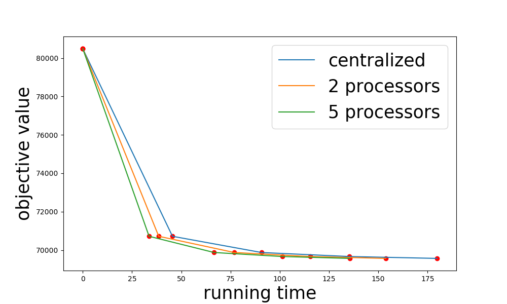
Figure 2 demonstrates how distributing the data among processors can speed up the convergence of the ADMM algorithm. In this experiment, we randomly generate a binomial graph with 100k nodes, 500k edges. Then we randomly generate the feature matrix and response vector for the graph. We test the model on a server with 12 processors, and we use the multiprocessing package from Python to control the number of processors used in the parallel computing paradigm. As can be seen from Figure 2, distributing the computation among processors can greatly reduce the running time. Note that the running time does not decrease proportionally to the number of processors. It is because Python multiprocessing module is used here, but it takes time for process to communicate with the memory, and only the step for updating is parallelled.
4.2 Latent Class Graph Regularization: Monte Carlo EM
Generally, graphical models with categorical latent variables can be solved using the expectation maximization (EM) algorithms. However, correlations among latent variables imposed by the social graph do not allow exact calculation of posterior distributions in the E-step using standard EM approaches. Instead, an approximate calculation of the E-step using Monte Carlo EM (MCEM) [23, 16, 7, 30] is employed. It is a modification of the original EM algorithm where the E-step is conducted approximately using a Monte Carlo Markov Chain (MCMC) algorithm. The details for each step of the MCEM algorithm for the proposed models are provided in the following subsections.
4.2.1 Expectation step
In this step the objective is to compute the marginal posterior distribution for nodes and edges, which will be used in the M-step to calculate the negative expected log-likelihood function. Refer to the Appendix for derivation of negative expected log-likelihood, which reveals the need for calculation of marginal posterior distributions.
In particular, for the E-step, one needs to calculate the following node marginal posterior probability
| (7) |
and the following edge posterior probability
| (8) | ||||
where represents the collection of parameters and . For small graphs, we can approximate the above distributions using standard MCMC algorithms. For large graphs, please refer to the Scalability of the E-step Subsection A in the Appendix.
4.2.2 Maximization step
Let us denote with and the marginal posterior distributions. The M-step of the EM algorithm requires minimizing the negative expected log-likelihood function
| (9) | ||||
where represents the collection of parameters and and . Derivation of this function is given in Subsection B in the Appendix. For small graphs, standard convex optimization solvers can be used. For large graphs, please refer to Section 4.1 where we discuss how we can maximize the expected log-likelihood efficiently with a distributed algorithm for LLGR. The objective function of the E step of LCGR model is the weighted version of the objective function of the LLGR model.
We now comment briefly on the theoretical asymptotic convergence of MCEM to a stationary point of the likelihood function. Convergence theory of MCEM in [23, 7] states that if standard MCMC is used in E step and that the MCMC sample size increases deterministically across MCEM iterations, then MCEM converges almost surely. We also consider using parallell block MCMC for large graphs (please refer to the Scalability of the E-step Subsection A in the Appendix), then a consequence of blocking of latent variables for the MCMC algorithm is that asymptotic convergence of MCEM is not guaranteed anymore. However, in practice, MCEM is often terminated without even knowing if the algorithm converges to an accurate solution. See for example Section in [23] and references therein about arbitrary termination criteria of MCEM. Therefore, we consider that the parallelism of block MCMC Algorithm in Subsection A of the Appendix, offers a trade-off between convergence and computational complexity per iteration by controlling the number of blocks, which in practice can speed up each iteration of the MCEM algorithm significantly.
5 Experiments
In this section, we analyze the empirical performance of the proposed social models on a range of datasets. We outline practical recommendations and illustrate examples where the proposed model is most suitable. The number of iterations of Gibbs sampler in the E-step grows with the number of iterations of the MCEM algorithm. The M-step is implemented using ECOS solver [9] embedded in CVXPY [8] for updates, bisection line search for updates, within ADMM iterations.
5.1 Illustrative Synthetic Data
We demonstrate that when graph structure and label assignment satisfy certain conditions, our LLGR and LCGR models performs better than other models without social information. We empirically illustrate the impact of graph structure by varying the connectivity between different classes in the graph, and illustrate the impact of label assignment by varying the discrepancies of labels in communities of the graph.
5.1.1 Varying connectivity between classes
We consider individuals, and use two different Gaussian distribution to generate feature vector for each individual. Then we randomly split the individuals into three communities with the same size. We assume that there are two classes, shown in blue and yellow in Figure 3. Notice that the feature vectors are assigned to communities regardless of their Gaussian distribution and labels are set based on the classes, which correspond to communities. Therefore, the labels are in align with the graph structure but not in align with the feature space. We set the probability of two individuals that are in the same community to get connected to , and the probability of two individuals that are in the same class but not in the same community to get connected to . Then we vary parameter , the probability of two individuals in different classes to get connected.
Figure 3shows the graph structure when , and . Notice that the larger is, the more edges among the communities belong in different classes. Table 2 shows the prediction result of four models as a function . Notice that since feature vectors and labels are not changed as changes, the prediction of logistic regression and logistic regression with latent class remains constant at . The reason that these models perform poorly is because the labels are not separable given the feature vectors only. Observe in Table 2 that when is as small as , which means that individuals in different classes are very unlikely to get connected, see Figure 3(a), the prediction result of the proposed social models is larger than . On the other hand, when becomes larger, the prediction of the social models is declining. However, as long as , the proposed LCGR model performs better than logistic regression and logistic regression with latent class models. When the social models has the same prediction performance as the logistic regression and latent class models. This is because the classes are not clearly separable on the graph, see Figure 3(c).


| model | |||||
|---|---|---|---|---|---|
| logistic reg. | 62% | 62% | 62% | 62% | 62% |
| log. reg. lat. class | 62% | 62% | 62% | 62% | 62% |
| LLGR | 80% | 62% | 62% | 62% | 62% |
| LCGR | 88% | 82% | 64% | 62% | 62% |
5.1.2 Varying choice preference parameters
An ideal scenario for the proposed social models is when classes correspond to communities of the given graph and when the labels are clustered according to the classes. However, labels might be misplaced in wrong classes. We study how the preference difference between classes affects the performance of the proposed model.
For this experiment individual feature vectors are generated from a Gaussian distribution with sample size . We randomly split this set of individuals into two parts with same size, and each part represents a class where individuals share the same parameters . Assume that is the weight corresponding to the th group, and . For each individual , is sampled from the same Gaussian distribution. For the graph setting, we set the probability of people in the same class to be connected as , and the probability of people in different classes to be connected as . This way, we ensure that classes correspond to communities.
Based on the data generation process, by tuning , we are able to get full control of preference difference among individuals in the two classes. When becomes larger, preference difference becomes larger as well. As we see in Figure 4, when becomes larger, more individuals in class one have (i.e., yellow squares) and more individuals in class two have have (i.e., turquoise triangles). When , around half of the individuals in both classes have , the other half , which means that there is no preference difference between the two classes. Prediction results for this experiment are shown in Table 3.
| model | ||||||
|---|---|---|---|---|---|---|
| logistic reg. | 48% | 44% | 42% | 52% | 58% | 52% |
| log. reg. lat. class | 48% | 48% | 54% | 54% | 42% | 36% |
| LLGR and LCGR | 100% | 100% | 94% | 86% | 68% | 36% |


5.2 Adolescent smoking
This example uses a dataset collected by [3]. This research program, known as the teenage friends and lifestyle study, has conducted a longitudinal survey of friendships and the emergence of the smoking habit (among other deviant behaviors) in teenage students across multiple schools in Glasgow, Scotland.
5.2.1 Dataset
Social graphs of students (shown in Figure 5) within the same age range of 13-15 years is constructed following a surveyed evidence of reciprocal friendship, with an edge placed among individuals and if individual and individual named each other friends. We included five variables into the feature vector : age; gender; money: indicating how much pocket money the student had per month, in British pounds; romantic: indicating whether the student is in a romantic relationship; family smoking: indicating whether there were family members smoking at home. Notice that the feature vectors and the edges of the graph are different at different timestamps. The response variable represents the stated choice that whether a student smokes tobacco (), otherwise . Note there are nodes with missing labels, but the graph structure should be intact for the parameter estimation of . Therefore, we set for these nodes, so that the corresponding are not used in the parameter estimation while keeping the graph structure unchanged.

127 non-smokers (blue),
23 smokers (red),
10 unobserved (yellow)
422 edges.

98 non smokers (blue),
39 smokers (red),
23 unobserved (yellow)
339 edges.
5.2.2 Models comparison
We measured predictions on this dataset and report here 3-fold cross validation results of four models: i) logistic regression; ii) latent class logistic regression; iii) social logistics regression, see Subsection 3.1; iv) social latent class logistics regression, see Subsection 3.2. Cross-validation process treats the removed nodes as nodes with missing labels, as described above. We consider latent classes in this experiment. The prediction performance is shown in Tables 4.
| model | 1995 | 1997 |
|---|---|---|
| logistic regression | 81.1% | 68.5% |
| latent class | 78.9% | 72.1% |
| LLGR | 80.0% | 76.9% |
| LCGR | 82.2% | 80.8% |
High performance of logistic regression and latent class model for the beginning of the study (Table 4) indicates that the smoking preferences are largely defined by individual feature vector. Moreover, parameters in the underlying classes of the latent class model don’t differ much. Social latent class model performs equally well. This difference grows significantly when a confounding variable of smoking in the family is removed from the feature list.
Furthermore, by the end of the study (January 1997, Table 4 column 2) one can see a significantly higher predictive accuracy of the LLGR and LCGR models. It may indicate that smoking within a certain group of teenagers have become a social norm (indicating the difference in offset parameters ), or that the response to independent factors within that group differs from the others as reflected by differences in .
Notice the significant decrease of prediction accuracy for non social models between column 1 and column 2 in Table 4. This is because at the beginning of the study (February ) less than of teenagers smoked, while at the end of the study (January ) about of teenagers smoked. This difference is likely due to social norms developed among teenagers that are captured by the graph and therefore missed by non social models.
5.2.3 Parameter visualization
We are going to illustrate how the specification of the proposed model allows in-depth exploration of the parameters to assist in making this type of conclusions. To that end, we are going to explore parameters and class membership probabilities across the regularization path of hyper-parameter .
The estimated class membership (the probability of being in a given latent class) on the graph is shown in Figure 6. A visualization of estimated of one latent class for several values of is shown in Figure 7. When , smoking pattern begins to show across the graph, i.e., compare Figures 5(b) and 7(b). Let us note that value corresponds to the best prediction accuracy in our experiments for the proposed social latent class logistic regression model for the smoke data at the end of the study (January ). This is because the social latent class logistic regression model is able to clearly distinguish a group of socially connected individuals within which the choice preferences towards smoking are higher.
When , are similar across the nodes. On the other hand, when , are not similar across the nodes. Although this is counter-intuitive since the graph regularization favors similar across nodes for large values of , it is explained by the node and edge posterior distribution in the M-step which also controls regularization across nodes during the execution of the algorithm.


5.3 Online Retail Account Relation Graph Data
In this section, we experimented our model on a real world online retail account relation graph from a leading commercial company in the US, and showed that our model excelled in fraud account prediction task when compared with other models. More details on the data and the empirical results have been redacted until their release has been approved
6 Conclusions and Future Work
In this paper we introduced social graph regularization ideas into discrete choice models for user choice modeling. We proposed local logistics graph regularization (LLGR) method and latent class graph regularization (LCGR) model. We developed scalable parameter estimation method for LLGR model on large graphs benefiting from recent advances in distributed optimization based on ADMM methods. Also we have developed, implemented, and explored parameter estimation algorithms that allow parallel processing implementation for both E- and M-steps of the Monte Carlo Expectation Maximization (MCEM) algorithms for LCGR model. In experimental evaluation, we have focused on investigating the usefulness of the models in revealing and supporting hypothesis in studies where not only predictive performance (that was found to be highly competitive), but also understanding social influence, is crucial. Our models can be directly applied to study social influence on revealed choices in large social graphs with rich node attributes. One challenge with extending our results is that such data are very rarely available in open access due to privacy issues.
Appendix A Improving E step
Here, we describe how to scale up the E step in Section 4.2.1, which is important for MCEM method, as described in Section 4.2. In the LCGR model, we use a markov random field to model the joint distribution of latent class conditioned on local coefficients . And we need to calculate the posterior node probabilities (Equation (7)) and edge probabilities (Equation (8)) in the E step based on Equation (4). Let us consider the case of two classes as an example. Assume the labels of the two classes are and , then we can simplify Equation (4) to
where we have and , and is the edge potentials. Thus, our model belongs to the standard pairwise Markov Random Field.
Both variational methods and sampling-based methods are suitable for our problem setting. (1) For variational methods, exact inference of Markov Random Field using Bethe approximation [32, 28] can calculate distributions of nodes and edges. The approximate inference algorithms, e.g., mean field inference [28] and loopy belief propagation (BP) [22], although exhibiting excellent empirical performance, is not calculated. (2) For sampling-based approach, MCMC algorithms can calculate both the node and edge distributions.
Calculating the marginal posterior probabilities Equation (7) and Equation (8) is computationally expensive due to the marginal probabilities and . This is because to calculate the latter two, we have to marginalize and latent variables, respectively. We chose sampling-based method and accelerated the computation by using a block MCMC sampling technique to compute and . The algorithm uses a preprocessing step to partition the graph into disjoint communities. Then it runs an MCMC algorithm on each community/block in parallel by ignoring the edges among the blocks.


Community Detection Result
Figure 8(a) demonstrates how parallel block MCMC speed up the computation. We use the Facebook Ego Network Data as shown in Figure 8(b), where there are 4039 nodes and 88234 edges. We randomly generate the local b value of each class for all the nodes. We first run Louvian community detection algorithm and extract 10 communities from the graph. We then run MCMC/ Block MCMC and Parallel Block MCMC and time the code for each iterations. As can be seen from Figure 8(a), the performance of MCMC and Block MCMC are almost the same, because the only difference is that Block MCMC omits the edges between communities for the Gibbs update. Since the MCMC update of each community is independent from each other, we can adopt the parallel computing paradigm for Block MCMC. As we can see from Figure 8(a), Parallel Block MCMC performs much better than the other two.
Appendix B Negative expected log-likelihood in Eq. (8)
We denote with the posterior distribution, with the sum over all latent variables , and represents the collection of parameters and . Let be the indicator function, which is equal to if . We assume that follows
| (10) |
and
| (11) |
where . The derivation of the expected log-likelihood is shown below.
We can exchange the sequence of and because each node can only be in one class, thus we have
Let’s write the summation over inside the summation over vertices and the summation over latent variables
and then we get the marginal probabilities
Using (11) and multiplying by minus equation we get the negative expected log-likelihood function in (9).
References
- [1] J. Abernethy, O. Chapelle and C. Castillo “Graph regularization methods for web spam detection” In Mach. Learn. 81.2, 2010, pp. 207–225
- [2] Reid Andersen, Fan Chung and Kevin Lang “Local graph partitioning using pagerank vectors” In Foundations of Computer Science, 2006. FOCS’06. 47th Annual IEEE Symposium on, 2006, pp. 475–486 IEEE
- [3] H Bush, Patrick West and Lynn Michell “The role of friendship groups in the uptake and maintenance of smoking amongst pre-adolescent and adolescent children: Distribution of Frequencies” In Glasgow, Scotland: Medical Research Council, 1997
- [4] Nicholas Christakis and James Fowler “Social contagion theory : examining dynamic social networks and human behavior”, 2013 DOI: 10.1002/sim.5408
- [5] H. Chung, B.. Flaherty and J.. Schafer “Latent class logistic regression: application to marijuana use and attitudes among high school seniors” In Journal of the Royal Statistical Society: Series A (Statistics in Society) 169.4, 2006, pp. 723–743
- [6] Micha\"el Defferrard, Xavier Bresson and Pierre Vandergheynst “Convolutional neural networks on graphs with fast localized spectral filtering” In Advances in Neural Information Processing Systems, 2016, pp. 3844–3852
- [7] B. Deylon, M. Lavielle and E. Moulines “Convergence of a Stochastic Approximation Version of the EM Algorithm” In The Annals of Statistics 27.1, 1999, pp. 94–128
- [8] Steven Diamond and Stephen Boyd “CVXPY: A Python-embedded modeling language for convex optimization” In Journal of Machine Learning Research 17.83, 2016, pp. 1–5
- [9] Alexander Domahidi, Eric Chu and Stephen Boyd “ECOS: An SOCP solver for embedded systems” In Control Conference (ECC), 2013 European, 2013, pp. 3071–3076 IEEE
- [10] Elenna Dugundji and Joan Walker “Discrete Choice with Social and Spatial Network Interdependencies: An Empirical Example Using Mixed Generalized Extreme Value Models with Field and Panel Effects” In Transp. Res. Rec. 1921.1, 2005, pp. 70–78 DOI: 10.3141/1921-09
- [11] David Gleich and Michael Mahoney “Using local spectral methods to robustify graph-based learning algorithms” In Proceedings of the 21th ACM SIGKDD International Conference on Knowledge Discovery and Data Mining, 2015, pp. 359–368 ACM
- [12] Aditya Grover and Jure Leskovec “node2vec: Scalable feature learning for networks” In Proceedings of the 22nd ACM SIGKDD international conference on Knowledge discovery and data mining, 2016, pp. 855–864 ACM
- [13] David Hallac, Jure Leskovec and Stephen Boyd “Network lasso: Clustering and optimization in large graphs” In Proceedings of the 21th ACM SIGKDD International Conference on Knowledge Discovery and Data Mining, 2015, pp. 387–396 ACM
- [14] Mikael Henaff, Joan Bruna and Yann LeCun “Deep convolutional networks on graph-structured data” In arXiv preprint arXiv:1506.05163, 2015
- [15] Thomas Kipf and Max Welling “Semi-supervised classification with graph convolutional networks” In arXiv preprint arXiv:1609.02907, 2016
- [16] R.. Levine and G. Casella “Implementations of the Monte Carlo EM Algorithm” In Journal of Computational and Graphical Statistics 10.3, 2012, pp. 422–439
- [17] H. Ma, D. Zhou, C. Liu, M.. Lyu and I. King “Recommender systems with social regularization” In WSDM ’11 Proceedings of the fourth ACM international conference on Web search and data mining, 2011, pp. 287–296
- [18] Charles. Manski “Identification of Social Endogenous Effects: The Reflection Problem” In Rev. Econ. Stud. 60.3, 1993, pp. 531–542 DOI: 10.2307/2298123
- [19] Tomas Mikolov, Ilya Sutskever, Kai Chen, Greg Corrado and Jeff Dean “Distributed representations of words and phrases and their compositionality” In Advances in neural information processing systems, 2013, pp. 3111–3119
- [20] Tomas Mikolov, Kai Chen, Greg Corrado and Jeffrey Dean “Efficient estimation of word representations in vector space” In arXiv preprint arXiv:1301.3781, 2013
- [21] Ben-Akiva Moshe, Bierlaire Michel, McFadden Daniel and Walker Joan “Discrete Choice Analysis”
- [22] Kevin Murphy, Yair Weiss and Michael Jordan “Loopy belief propagation for approximate inference: An empirical study” In Proceedings of the Fifteenth conference on Uncertainty in artificial intelligence, 1999, pp. 467–475 Morgan Kaufmann Publishers Inc.
- [23] Ronald Neath “On convergence properties of the Monte Carlo EM algorithm” In Advances in Modern Statistical Theory and Applications: A Festschrift in Honor of Morris L. Eaton Institute of Mathematical Statistics, 2013, pp. 43–62
- [24] Bryan Perozzi, Rami Al-Rfou and Steven Skiena “Deepwalk: Online learning of social representations” In Proceedings of the 20th ACM SIGKDD international conference on Knowledge discovery and data mining, 2014, pp. 701–710 ACM
- [25] K. Roeder, K.. Lynch and D.. Nagin “Modeling Uncertainty in Latent Class Membership: A Case Study in Criminology” In Journal of the American Statistical Association 94.447, 1999, pp. 766–776
- [26] Cr Shalizi and Ac Thomas “Homophily and contagion are generically confounded in observational social network studies” In Sociol. Methods Res., 2011, pp. 1–27 arXiv: http://smr.sagepub.com/content/40/2/211.short
- [27] Jian Tang, Meng Qu, Mingzhe Wang, Ming Zhang, Jun Yan and Qiaozhu Mei “Line: Large-scale information network embedding” In Proceedings of the 24th International Conference on World Wide Web, 2015, pp. 1067–1077 International World Wide Web Conferences Steering Committee
- [28] Martin Wainwright and Michael Jordan “Graphical models, exponential families, and variational inference” In Foundations and Trends® in Machine Learning 1.1–2 Now Publishers, Inc., 2008, pp. 1–305
- [29] J.. Walker and J. Li “Latent lifestyle preferences and household location decisions” In Journal of Geographical Systems 9.1, 2007, pp. 77–101
- [30] G…G. Wei and M.. Tanner “A Monte Carlo Implementation of the EM Algorithm and the Poor Man’s Data Augmentation Algorithms” In Journal of the American Statistical Association 85.411, 1990, pp. 699–704
- [31] Derry Wijaya, Partha Talukdar and Tom Mitchell “Pidgin: ontology alignment using web text as interlingua” In Proceedings of the 22nd ACM international conference on Information & Knowledge Management, 2013, pp. 589–598 ACM
- [32] Alan Willsky, Erik Sudderth and Martin Wainwright “Loop series and Bethe variational bounds in attractive graphical models” In Advances in neural information processing systems, 2008, pp. 1425–1432
- [33] Zhilin Yang, William Cohen and Ruslan Salakhutdinov “Revisiting semi-supervised learning with graph embeddings” In arXiv preprint arXiv:1603.08861, 2016
- [34] Denny Zhou, Olivier Bousquet, Thomas Lal, Jason Weston and Bernhard Sch\"olkopf “Learning with local and global consistency” In Advances in neural information processing systems, 2004, pp. 321–328
- [35] Xiaojin Zhu, Zoubin Ghahramani and John Lafferty “Semi-supervised learning using gaussian fields and harmonic functions” In Proceedings of the 20th International conference on Machine learning (ICML-03), 2003, pp. 912–919