Tetrahedral mesh improvement using moving mesh smoothing, lazy searching flips, and RBF surface reconstruction
Abstract
Given a tetrahedral mesh and objective functionals measuring the mesh quality which take into account the shape, size, and orientation of the mesh elements, our aim is to improve the mesh quality as much as possible. In this paper, we combine the moving mesh smoothing, based on the integration of an ordinary differential equation coming from a given functional, with the lazy flip technique, a reversible edge removal algorithm to modify the mesh connectivity. Moreover, we utilize radial basis function (RBF) surface reconstruction to improve tetrahedral meshes with curved boundary surfaces. Numerical tests show that the combination of these techniques into a mesh improvement framework achieves results which are comparable and even better than the previously reported ones.
Keywords:
mesh improvement , mesh quality , edge flipping , mesh smoothing , moving mesh , radial basis functions2010 MSC
65N50 , 65M50 , 65L50 , 65K101 Introduction
The key mesh improvement operations considered in this work are smoothing, which moves the mesh vertices, flipping, which changes the mesh topology without moving the mesh vertices, and a smooth boundary reconstruction. Previous work shows that the combination of smoothing and flipping achieves better results than if applied individually [1, 2]. In this paper, we combine the recently developed flipping and smoothing methods into one mesh improvement scheme and apply them in combination with a smooth boundary reconstruction via radial basis functions.
Mesh smoothing improves the mesh quality by improving vertex locations, typically through Laplacian smoothing or some optimization-based algorithm. Most commonly used mesh smoothing methods are Laplacian smoothing and its variants [3, 4], where a vertex is moved to the geometric center of its neighboring vertices. While economic, easy to implement, and often effective, Laplacian smoothing guarantees neither a mesh quality improvement nor mesh validity. Alternatives are optimization-based methods that are effective with respect to certain mesh quality measures such as the ratio of the area to the sum of the squared edge lengths [5], the ratio of the volume to a power of the sum of the squared face areas [6], the condition number of the Jacobian matrix of the affine mapping between the reference element and physical elements [7], or various other measures [1, 8, 9, 10]. Most of the optimization-based methods are local and sequential, combining Gauss-Seidel-type iterations with location optimization problems over each patch. There is also a parallel algorithm that solves a sequence of independent subproblems [11].
In our scheme, we employ the moving mesh PDE (MMPDE) method, defined as the gradient flow equation of a meshing functional (an objective functional in the context of optimization) to move the mesh continuously in time. Such a functional is typically based on error estimation or physical and geometric considerations. Here, we consider a functional based on the equidistribution and alignment conditions [12] and employ the recently developed direct geometric discretization [13] of the underlying meshing functional on simplicial meshes. Compared to the aforementioned mesh smoothing methods, the considered method has several advantages: it can be easily parallelized, it is based on a continuous functional for which the existence of minimizers is known, the functional controlling the mesh shape and size has a clear geometric meaning, and the nodal mesh velocities are given by a simple analytical matrix form. Moreover, the smoothed mesh will stay valid if it was valid initially [14].
Flipping is the most efficient way to locally improve the mesh quality and it has been extensively addressed in the literature [15, 1, 16, 2]. In the simplest case, the basic flip operations, such as 2-to-3, 3-to-2, and 4-to-4 flips, are applied as long as the mesh quality can be improved. The more effective way is to combine several basic flip operations into one edge removal operation, which extends the 3-to-2 and 4-to-4 flips. This operation removes the common edge of adjacent tetrahedra by replacing them with new tetrahedra (the so-called -to- flip). There are at most possible variants to remove an edge by a -to- flip, where is the Catalan number. If is small (e.g., ), one can enumerate all possible cases, compute the mesh quality for each case, and then pick the optimal one. Another way is to use dynamic programming to find the optimal configuration. However, the number of cases increases exponentially and finding the optimal solution with brute force is very time-consuming.
In this paper, we propose the so-called lazy searching flips. The key idea is to automatically explore sequences of flips to remove a given edge in the mesh. If a flip sequence leads to a configuration which does not improve the mesh quality, the algorithm reverses this sequence and explores another one (see sections 3, 2(a), 2(c) and 2(b)). Once an improvement is found, the algorithms stops the search and returns without exploring the remaining possibilities.
When considering more arbitrary meshes (which may not be piecewise planar), we need to make sure that new nodes are added in a consistent way. To achieve this we use RBF surface reconstruction as introduced in [17]. Radial basis functions are a very useful tool in the context of higher-dimensional interpolation as they dispense with the expensive generation of a mesh [18, 19, 20]. Here, we will employ them to approximate the underlying continuous surface so that we can project nodes onto it as proposed in [21, 22]. This problem turns out to be very challenging for meshes with arbitrary boundary. Hence, we begin with a relatively simple mesh. For more complicated examples we first refine the boundary by using the RBF reconstruction and projection method and then keep the boundary nodes fixed while interior nodes may move.
In this paper, we provide a detailed numerical study of a combination of the MMPDE smoothing with the lazy searching flips and RBF surface reconstruction. More specifically, we compare the results of the whole algorithm with Stellar [2], CGAL [23] and mmg3d [24]. We also compare the lazy searching flips and the MMPDE smoothing with the flipping and smoothing procedures provided by Stellar.
2 The moving mesh PDE smoothing scheme
The key idea of this smoothing scheme is to move the mesh vertices via a moving mesh equation, which is formulated as the gradient system of an energy functional (the MMPDE approach). Originally, the method was developed in the continuous setting [25, 26]. In this paper, we use its discrete form [13, 14, 27], for which the mesh vertex velocities are expressed in a simple, analytical matrix form, which makes the implementation more straightforward to parallelize.
2.1 Moving mesh smoothing
Consider a polygonal (polyhedral) domain with . Let denote the simplicial mesh as well as and the numbers of its vertices and elements, respectively. Let be a generic mesh element and the reference element taken as a regular simplex with volume . Further, let be the Jacobian matrix of the affine mapping from the reference element to a mesh element . For notational simplicity, we denote the inverse of the Jacobian by , i.e., (see fig. 1).
Then, the mesh is uniform if and only if
| (1) |
The first condition requires all elements to have the same size and the second requires all elements to be shaped similarly to (these conditions are the simplified versions of the equidistribution and alignment conditions [28, 26]).
The corresponding energy functional for which the minimization will result in a mesh satisfying eq. 1 as closely as possible is
| (2) |
with
| (3) |
where and are dimensionless parameters (in section 6, we use and ). This is a specific choice and other meshing functionals are possible. The interested reader is referred to [29] for a numerical comparison of meshing functionals for variational mesh adaptation.
In eq. 2, is a Riemann sum of a continuous functional for variational mesh adaptation based on equidistribution and alignment [12] and depends on the vertex coordinates , . The corresponding vertex velocities for the mesh movement are defined as
| (4) |
where the derivatives are considered to be row vectors.
2.2 Vertex velocities and the mesh movement
The vertex velocities can be computed analytically [13, Eqs (39) to (41)] using scalar-by-matrix differentiation [13, Sect. 3.2]. Denote the vertices of and by and , , and define the element edge matrices as
Note, that . Then, the local mesh velocities are given element-wise [13, Eqs (39) and (41)] by
| (5) | ||||
where and
are the derivatives of with respect to its first and second argument [13, Example 3.2] evaluated at and .
The moving mesh equation (4) becomes
| (6) |
where is the patch of the vertex and is the local index of on .
The moving mesh governed by eq. 6 will stay nonsingular if it is nonsingular initially: the minimum height and the minimum volume of the mesh elements will stay bounded from below by a positive number depending only on the initial mesh and the number of the elements [14]. This holds for the numerical integration of eq. 6 as well if the ODE solver has the property of monotonically decreasing energy [14]. For example, algebraically stable Runge-Kutta methods preserve this property under a mild step-size restriction [30].
During smoothing, we use the current vertex locations as the initial position and integrate eq. 6 for a time period (with the proper modification for the boundary vertices, see section 2.3). The connectivity is kept fixed during the smoothing step. The time integration can be carried out for a given fixed time period or adaptively until the change of the energy functional (2) is smaller than the prescribed absolute or relative tolerances, that is until
2.3 Velocity adjustment for the boundary vertices
The velocities of the boundary vertices need to be modified. If is a fixed boundary vertex, then its velocity is set to zero Otherwise, is allowed to move along a boundary curve or a surface represented by the zero level set of a function and its velocity is modified so that its normal component along the curve (surface) is zero:
For the special case of a piecewise linear complex (PLC) [32] the velocity adjustment is straightforward:
| facet vertices: | project the velocity onto the facet plane, | ||
| segment vertices: | project the velocity onto the segment line, | ||
| corner vertices: | set the velocity to zero. |
For a general non-polygonal or non-polyhedral domain, a simple way to adjust the boundary vertices is to move the vertex and then project it onto the boundary to which it belongs, which proved to work well for simple surface geometries (see section 6.2). However, for complicated geometries, this simple projection can fail and a more reliable approach is needed.
3 Lazy searching flips
In this section, we explain how to remove an edge and how to reverse the removal using flips. In addition, we present the lazy searching algorithm which can be used to improve the quality of a mesh.
3.1 Edge removal and its inverse
A basic edge removal algorithm performs a sequence of elementary 2-to-3 and 3-to-2 flips [33]. We extend this algorithm by allowing the flip sequence to be reversed. Our algorithm saves the flips online and it uses no additional memory.
Let be an edge with endpoints and and be the array of tetrahedra in sharing . For simplicity, we assume that is an interior edge of , so that all tetrahedra in can be ordered cyclically such that the two tetrahedra and share a common face. The index takes values in . Throughout this section, additions involving indices will be modulo .
Given such an array of tetrahedra, we want to find a sequence of flips that will remove the edge . Moreover, we also want to be able to reverse this sequence in order to return to the original state.
Our edge removal algorithm includes two subroutines
with an array (of length ) of tetrahedra and an integer level defining the maximum recursive level as input.
- flipnm
-
executes “forward” flips to remove the edge . It returns a Boolean value indicating whether the edge is removed or not and an integer (). If the edge is not removed (), indicates the current size of (initially, ).
- flipnm_post
-
must be called immediately after flipnm. It releases the memory allocated in flipnm and can perform “backward” flips to undo the flip sequence performed by flipnm.
The basic subroutine flipnm consists of the following three steps:
- 1.
Return if and flip32 is possible for and otherwise.
- 2.
For each try to remove the face by flip23. If it is successfully flipped, reduce the size of by . Update so that it contains the current set of tetrahedra sharing the edge . Reuse the last entry, , to store the information of this flip23 (see Figure 2(c)). It then (recursively) calls . When no face can be removed, go to Step 3.
- 3.
If , try to remove an edge adjacent to using flipnm. For each , let be given by either edge or edge . Initialize an array of tetrahedra sharing and call flipnm. If is successfully removed, reduce by . Update to contain the current set of tetrahedra sharing the edge . Reuse the last entry, , to store the information of this flipnm and the address of the array (to be able to release the occupied memory later). Then (recursively) call . Otherwise, if is not removed, call flipnm_post to free the memory. Return if no edge can be removed.
Since flipnm is called recursively, not every face and edge should be flipped in Steps 2 and 3. In particular, if is allocated, i.e., flipnm is called recursively, we skip flipping faces and edges belonging to the tetrahedra in .
In the simplest case, that is, ignoring the option to reverse the flips, flipnm_post simply walks through the array from to and checks if a flipnm flip has been saved. If so, the saved array address is extracted and its memory is released.
In Step 2 there are at most different flip sequences, depending on the specific choice of faces in . Each individual flip sequence is equivalent to a sequence of the vertices (apexes) in the link of the edge . We reuse the entries of to store each flip sequence. After a 2-to-3 flip, the number of the tetrahedra in array is reduced by one (two tetrahedra out, one terahedron in), since only one of the three new tetrahedra contains the edge . The remaining tetrahedra are shifted by one in the list, so that the last entry, , can be used to store this flip (cf. fig. 2(c)). In particular, the following information is saved:
- 1.
a flag indicating a 2-to-3 flip;
- 2.
the original position , meaning that the face is flipped.
Both is compressed and stored in the entry (note that a flag requires just a few bits of space). This stored data allows us to perform the reversal of a 2-to-3 flip as follows:
- 1.
use and the position with
to locate the three tetrahedra sharing the edge : , , and ;
- 2.
perform a 3-to-2 flip on these three tetrahedra;
- 3.
insert two new tetrahedra into the array :
In Step 3, if the selected edge is removed, the sequence of flips to remove is stored in . We then use the last entry to store this sequence of flips. In particular, the following information is saved:
- 1.
a flag indicating that this entry stores the flip sequence to remove the edge ;
- 2.
the original position , i.e., the edge is flipped;
- 3.
the address of the array which stores the flip sequence.
This information allows us to reverse this sequence of flips exactly.


 |
 |
 |
 |
| (1) | (2) | (3) | (4) |
 |
 |
 |
 |
| (5) | (6) | (7) | (8) |
3.2 Lazy searching flips
During the mesh improvement process we perform flips to improve the mesh quality. Let us consider the case when it becomes necessary to remove an edge. The maximum possible number of flips for an edge removal is the Catalan number ( is the size of ). Hence, the direct search for the optimal solution is only meaningful if is very small. In most situations, an edge may not be flipped if we restrict ourselves to adjacent faces of the edge. Our strategy is to search and perform the flips as long as they improve the current mesh quality. Our lazy searching scheme is not restricted by the number and can be extended to adjacent edges.
The lazy searching flip scheme is like a walk in a -ary search tree (a rooted tree with at most children at each node, see fig. 2(b)). The root represents the edge to be flipped and each of the tree nodes represents either an adjacent face or an adjacent edge or of . The edges of the tree represent our search paths. In particular, the directed edge from level to represents either a flip23 or a flipnm, and the reversed edge represents the inverse operation. The tree depth is given by the parameter level.
At , in order to to decide if an adjacent face should be flipped, we check if is flippable and make sure that this flip improves the local mesh quality. Note that we need to check only two of the three new tetrahedra: and . The tetrahedron will be involved in the later flips, and will be flipped if the edge is flipped.
Once an improvement is found, the algorithm moves on to the next edge without exploring other possibilities.
4 Radial basis functions to handle curved boundaries
We describe in this section how to project the mesh on a smooth surface in order to deal with curved boundaries. We achieve this with the help of radial basis functions (RBFs), see [18, 19, 20].
4.1 Basic concepts and examples
Let denote the space of variate polynomials with absolute degree at most and dimension . For a basis of this space, define the polynomial matrix through its entry,
where and denotes a data set. The function is called conditionally positive definite of order m if the quadratic form
for the distance matrix with its entry defined by
is positive for all data sets and for all which additionally satisfy the constraint .
Conditionally positive functions of order are also conditionally positive definite for any order higher than . Hence, the order shall denote the smallest positive integer . A conditionally positive definite function of order is called positive definite.
One speaks of radial basis functions if one additionally assumes that is a radial function, i.e., there exists a function such that . Common examples of RBFs include:
| Gaussian: | |||
| Multiquadric: | |||
| Inverse Multiquadric: | |||
| Polyharmarmonic Spline: |
For the numerical examples in this paper, we exclusively use the polyharmonic spline (fig. 3) which is conditionally positive of order 2.

We assume now that the interpolant is given by a linear combination of translated radial basis function, augmented by a polynomial part, i. e.
| (7) |
Thus, we have unknown coefficients, of which are determined from the interpolation conditions and conditions from requiring that . For positive definite functions, the linear system is positive definite by construction. Hence the coefficients can be determined uniquely. It is also not difficult to verify that the interpolation and polynomial constraint conditions for conditionally positive definite functions lead to a uniquely solvable system, see [20, Theorem 8.21] for details. In the case of conditionally positive definite functions, it is known that at least eigenvalues of the matrix are positive [20, Section 8.1].
4.2 Surface reconstruction with RBFs
We will assume that the surface is given implicitly by the zero level set of some function , i. e.
| (8) |
for some bounded domain .
We cannot simply assume that the target function (which we wish to interpolate) is the zero level set of the function since the right-hand side of the linear system one needs to solve would vanish which in turn implies that the coefficients vanish as well. Carr et al. [17] therefore made the additional assumption that the normal vectors are known. Then one can also prescribe on-surface and off-surface points. Assume that the points on the surface are denoted with and the corresponding normal vectors with . We define the surface interpolation problem
| (9) | ||||||
for some parameter . Since the right-hand side of the linear system does not vanish anymore, we find a nontrivial solution. Recently, this surface interpolation technique was combined with the higher dimensional embedding technique [21, 22] to construct curvature-aligned anisotropic surface meshes. In this context the data set corresponds to the vertices of the mesh.
4.3 Projection onto the reconstructed surface
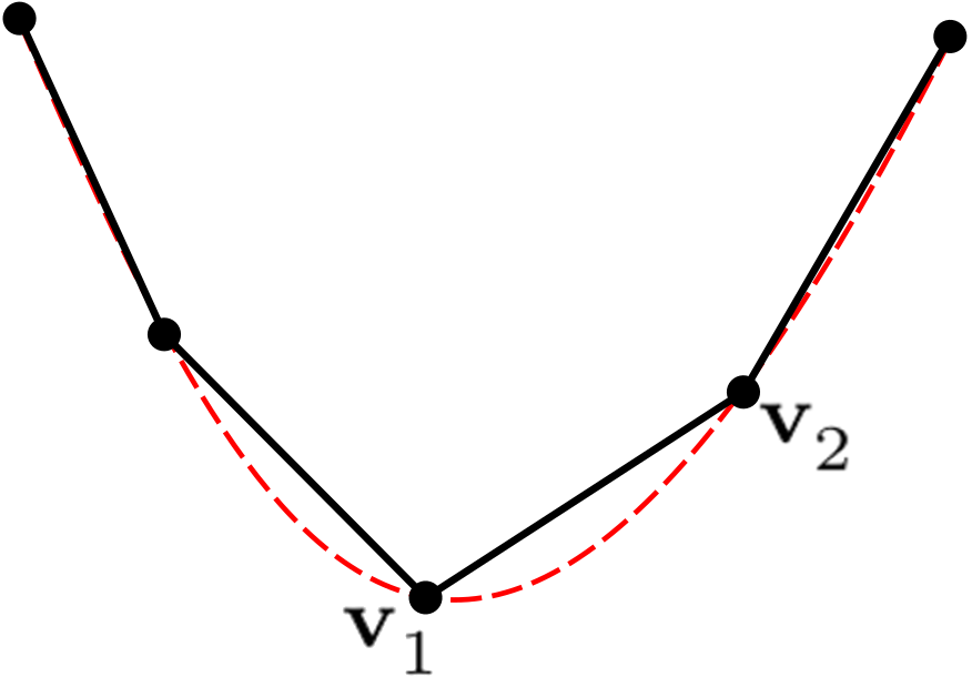
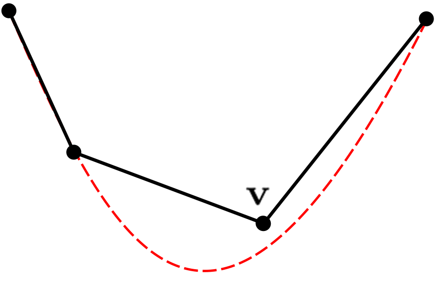
There are two important parts of the projection algorithm: edge splitting and edge contraction. If we split an edge or move a point during smoothing, we project the resulting point onto the RBF surface reconstruction (fig. 4).


The projection itself is realized with ideas from [34]. This procedure is a combination of orthogonal projections on tangent planes as well as tangent parabolas. It requires only first order derivatives and uses a steepest descent method. The combination of this projection method with RBF surface reconstruction has also been discussed in [21, 22].
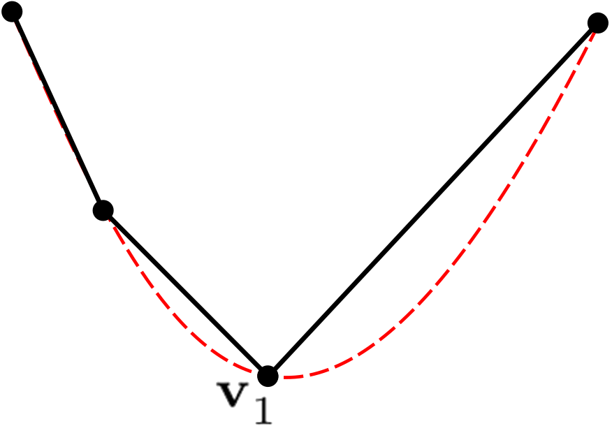
When it becomes necessary to contract an edge, we contract it into one of its endpoints (fig. 5).
5 Mesh improvement strategy
The goal of the proposed algorithm is to obtain a new isotropic mesh whose elements come “as close as possible” to the equilateral one. To achieve this goal, we combine the local and global mesh operations described in sections 2 and 3.
5.1 Mesh quality
To say “as close as possible to an equilateral tetrahedron” is somewhat vague from a mathematical point of view. To have a more precise criterion, the majority of the mesh improvement algorithms define a computable quantity which quantifies how far a tetrahedron is from being equilateral [2, 24, 35, 36, 37, 38]. Here, we take into account the following two:
- Aspect Ratio:
-
This is one of the most classical ways to evaluate the quality of a tetrahedron. It is defined as
(10) where is the longest edge and is the shortest altitude of the tetrahedron . By construction, and an equilateral tetrahedron is characterized by .
- Min-max Dihedral Angle:
-
For each tetrahedron we consider both the minimal and the maximal dihedral angles and . An equilateral tetrahedron has . Applying an operation that increases or decreases of a given tetrahedron makes “closer” to the equilateral shape. Note that this is not a classical quality measure since we associate two quantities with each tetrahedron, which is one of the novel aspects of the proposed mesh improvement procedure.
These two quality measures refer to a single tetrahedron of the mesh. However, the design of our mesh improvement scheme requires a quality measure for the whole mesh as a stopping criterion. To estimate the quality of the whole mesh, we define the global parameter
| (11) |
If we consider a target dihedral angle and obtain a mesh with , then all dihedral angles are guaranteed to be greater than .
5.2 The scheme
The inputs for the mesh improvement algorithm are a tetrahedral mesh of a PLC and a target minimum angle . The output is a mesh where each element has a minimum dihedral angle greater than .
Improve,
The scheme is presented in Algorithm 1 and consists of five nested “repeat … until” loops, whose stopping criterion depends on the operations done inside the loop and . We apply the MMPDE smoothing and the lazy flip in the most internal loop (5 to 9). The lazy flip is also exploited in the outer loops both on the whole mesh (11, 15 and 18) and on the tetrahedra involved in the local operations (10, 13 and 17).
It is possible to consider several flipping criteria for the lazy flip, which makes the design of the scheme flexible. We exploit this feature by using two objective functionals and changing the flipping criterion in each iteration of the outer loop (20) by
- 1.
maximizing and minimizing (simultaneously),
- 2.
minimizing the aspect ratio.
The stopping criterion is always based on the minimal dihedral angle, , and the number of operations done.
After a number of iterations both the flipping and the smoothing procedure can stagnate, i.e., the mesh converges to a fixed configuration where neither flips nor smoothing can improve the quality of the mesh. Unfortunately, it is not a priori guaranteed that such a mesh satisfies the constraint on the target minimum dihedral angle . To overcome this difficulty, we apply edge splitting, edge contraction, and point insertion when this stagnation occurs (10, 13 and 17 in Algorithm 1).
For the edge contraction and splitting, we use the standard edge length criterion: we compute the average edge length of the actual mesh, contract the edges shorter than (10), and split (halve) the ones longer than (13). In 17, we split a tetrahedron with via a standard 1-to-4 flip by placing the newly added point at the barycenter of [39]. In this way, the algorithm constructs via flipping and smoothing a mesh satisfying . At the moment, we are not interested in optimizing these operations, we exploit them only to overcome the stagnation of the algorithm.
The MMPDE smoothing can be easily parallelized because the nodal velocities in each smoothing step can be assembled through independent element-wise computation (eqs. 5 and 6), similar to the assembly of a finite element stiffness matrix. We parallelize the computation of the nodal velocities with OpenMP [40]. Once the velocities are computed, all mesh nodes are moved simultaneously and independently of each other. On the other hand, the lazy flip may propagate to neighbors and neighbors of neighbors, thus, it is complex and difficult to parallelize; in our tests we use a sequential implementation.
6 Numerical examples
We test the proposed mesh improvement algorithm and compare it with the mesh improvement algorithm of Stellar [2], the remeshing procedure of CGAL [23], and mmg3d [24]. We compare the histograms of the dihedral angles of final meshes, the minimal and the maximal dihedral angles and , the mean dihedral angle , and its standard deviation .
6.1 Piecewise linear complexes (PLCs)
To analyze the effectiveness of the proposed mesh improvement scheme in case of a piecewise linear complex domain, we consider the following three examples (for more PLC examples, see [41]):
- 1.
- 2.
- 3.
TetgenExample is a tetrahedral example mesh of a non-convex PLC with a hole provided by TetGen (fig. 9).
Smoothing and flipping by themselves
Before testing the full mesh improvement scheme, we test the effectiveness of the MMPDE smoothing and the lazy flip by themselves and employ smoothing and flipping separately, i.e., we improve a tetrahedral mesh exploiting only the flipping operation or the vertex smoothing. We compare our results with the ones provided by Stellar for the examples LShape and TetGenExample.
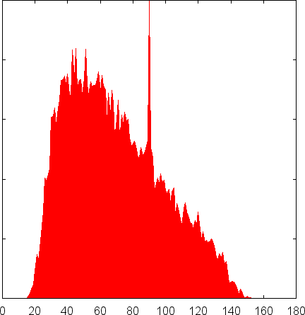
The results of the lazy flip are comparable to the Stellar flips (fig. 6, first row). However, the MMPDE smoothing is better than its counterpart in Stellar (fig. 6, second row): in both examples it achieves larger , noticeably smaller , and a smaller standard deviation of the mean dihedral angle.
Lazy Flip

Stellar flipping

MMPDE smoothing

Stellar smoothing

Lazy Flip

Stellar flipping

MMPDE smoothing

Stellar smoothing
Full scheme
We compare the whole scheme with the mesh improvement algorithm of Stellar [2], the remeshing procedure of CGAL [23], and mmg3d [24] (figs. 7, 8 and 9).
Although all methods provide good results, the new scheme is better: is larger than the value obtained by CGAL or mmg3d and comparable to the value obtained by Stellar. Moreover, is smaller than the values obtained by Stellar, CGAL, or mmg3d in all examples but one see fig. 9(a).
Initial Mesh New Method


New Method
 Stellar
 CGAL
CGAL
 mmg3d
mmg3d

Initial Mesh New Method


New Method
 Stellar
 CGAL
CGAL
 mmg3d
mmg3d

Initial Mesh New Method


New Method

Stellar

CGAL

MMG3

New Method

Stellar

CGAL

mmg3d

Our method provides mean dihedral angles around , which is close to the optimal value of . Moreover, standard deviations are always smaller than the ones of other methods. Indeed, we get a distribution of dihedral angles close to the mean value. This quantitative consideration becomes clearer from the shape of the histograms in figs. 7, 8 and 9.
For the TetgenExample (fig. 9) we also provide aspect ratio histograms (the results for the other examples are very similar and we omit them). The aspect ratio of an equilateral tetrahedron is equal to and the more a tetrahedron is distorted and stretched the greater its aspect ratio becomes. Our method and Stellar clearly provide the best aspect ratio distribution. For our method, the vast majority of tetrahedra have an aspect ratio smaller than . The Stellar mesh is slightly worse with most of its tetrahedra having aspect ratios below .
6.2 Curved boundary domains
In the last part of this section, we experimentally demonstrate some examples with curved domains. We study two types of examples: one academic example for using the RBF surface reconstruction to project the boundary vertices on the smooth approximation of the discrete surface and two more complex examples with fixed boundary vertices.
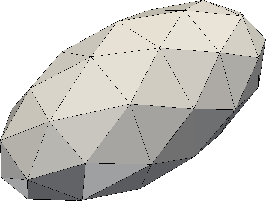
First, we consider the discrete ellipsoid mesh (fig. 10). Though it has a simple geometry, it requires some effort since the boundary is curved and no longer a PLC. The main challenge is to project the boundary vertices back onto the smooth surface if they leave it after a mesh improvement step. For this reason, we reconstruct the surface via RBFs (see section 4.2) to assist the mesh optimization and project the moved (smoothed) boundary vertices to the reconstructed surface.
Initial
Final

Cross section

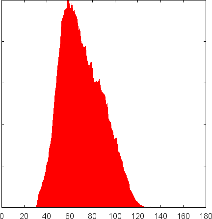
Figure 10 shows that RBF reconstruction smoothes the initially rough surface approximation. The obtained tetrahedral mesh has high quality: the mean dihedral angle is close to the optimal value () and the standard deviation of the dihedral angles is small ().
However, it has to be pointed out that complicated boundaries cannot be handled as easily as an ellipsoid and require more sophisticated methods.
In our next examples, we restrict ourselves to the case of fixed boundary vertices since Stellar does not handle curved surfaces described via an implicit function, start with a good isotropic triangular mesh as input, and keep the boundary vertices fixed for each of the algorithms.
Fixed boundary
The next two examples are meshes of a spinal bone and of an elephant (figs. 11 and 12). The initial surface meshes in both examples are constructed by means of the higher dimensional embedding approach for surface mesh reconstruction [22] and their minimal face angles are approximately . The initial volume meshes are constructed by TetGen using the -Y flag to preserve the fixed boundary.
Figures 11 and 12 present the histograms of the dihedral angles of the resulting optimized meshes. In comparison to the PLC examples, where the geometry is simpler and the boundary vertices are allowed to move, the smallest dihedral angles for the spinal bone and the elephant examples are worse (smaller) than for the PLC examples. In comparison to Stellar, our algorithm achieves better values for and , as well as a smaller mean deviation from the mean value.
These examples, too, show the “aggressive” nature of the Stellar mesh improvement algorithm, which aggressively removes vertices during the mesh improvement. In contrast, our mesh improvement scheme is able to produce a high-quality mesh while keeping the number of vertices close to the original input.
Surface mesh

Cross section

New Method

Stellar

Surface mesh

Cross section

New Method

Stellar

7 Conclusions
Mesh improvement is a challenging problem and we tackled it by combining several recently developed techniques, namely, moving mesh smoothing, lazy flipping, and RBF surface reconstruction. In comparison to the mesh improvement algorithm Stellar and the re-meshing procedures provided by CGAL and mmg3d, we obtain better results in terms of the distributions of dihedral angles for all considered examples. However, there are several directions in which this work could be extended.
First, for smooth and relatively simple boundaries, our approach works excellently but complicated curved boundaries pose a challenging problem. One possible solution could be the direct incorporation of the boundary description into the MMPDE smoothing scheme (parametrization) so that the boundary vertices will always stay on the surface. This will avoid the sometimes troublesome projection of vertices and velocities back onto the surface after a smoothing step.
Second, we need to find a more sophisticated method for edge contraction and splitting in order to improve the performance of both the MMPDE smoothing and the lazy flip.
Third, the MMPDE smoothing is based on the moving mesh method [13] which allows the definition of a metric field. Hence, the moving mesh smoothing can be extended to the adaptive and anisotropic setting.
Acknowledgments
The work of Franco Dassi was partially supported by the “Leibniz-DAAD Research Fellowship 2014”. The authors are thankful to Jeanne Pellerin for her support in computing the examples with mmg3d [24] and the anonymous referee for the valuable comments which helped to improve the quality of this paper.
References
- [1] L. A. Freitag, C. Ollivier-Gooch, Tetrahedral mesh improvement using swapping and smoothing, Internat. J. Numer. Methods Engrg. 40 (21) (1997) 3979–4002.
- [2] B. M. Klingner, J. R. Shewchuk, Aggressive tetrahedral mesh improvement, in: Proceedings of the 16th International Meshing Roundtable, 2007, pp. 3–23, http://graphics.cs.berkeley.edu/papers/Klingner-ATM-2007-10.
- [3] D. A. Field, Laplacian smoothing and Delaunay triangulations, Comm. Appl. Num. Meth. 4 (1978) 709–712.
- [4] S. H. Lo, A new mesh generation scheme for arbitaar planar domains, Int. J. Numer. Meth. Engng. 21 (1985) 1403–1426.
- [5] R. E. Bank, PLTMG: a software package for solving elliptic partial differential equations, Vol. 15 of Frontiers in Applied Mathematics, Society for Industrial and Applied Mathematics (SIAM), Philadelphia, PA, 1994, users’ guide 7.0.
- [6] M. Shephard, M. Georges, Automatic three-dimensional mesh generation by the finite octree technique, Int. J. Numer. Meth. Engrg. 32 (1991) 709–749.
- [7] L. A. Freitag, P. M. Knupp, Tetrahedral mesh improvement via optimization of the element condition number, Internat. J. Numer. Methods Engrg. 53 (6) (2002) 1377–1391.
- [8] P. M. Knupp, Achieving finite element mesh quality via optimization of the Jacobian matrix norm and associated quantities. Part I – A framework for surface mesh optimization, Internat. J. Numer. Methods Engrg. 48 (2000) 401–420.
- [9] P. M. Knupp, Applications of mesh smoothing: copy, morph, and sweep on unstructured quadrilateral meshes, Internat. J. Numer. Methods Engrg. 45 (1) (1999) 37–45.
- [10] S. A. Canann, J. R. Tristano, M. L. Staten., An approach to combined Laplacian and optimization-based smoothing for triangular, quadrilateral, and quad-dominant meshes, in: Proceedings of the 7th International Meshing Rountable (1998).
- [11] L. Freitag, M. Jones, P. Plassmann, A parallel algorithm for mesh smoothing, SIAM J. Sci. Comput. 20 (6) (1999) 2023–2040.
- [12] W. Huang, Variational mesh adaptation: isotropy and equidistribution, J. Comput. Phys. 174 (2) (2001) 903–924.
- [13] W. Huang, L. Kamenski, A geometric discretization and a simple implementation for variational mesh generation and adaptation, J. Comput. Phys. 301 (2015) 322–337.
- [14] W. Huang, L. Kamenski, On the mesh nonsingularity of the moving mesh PDE method, Math. Comp. (electronically). doi:10.1090/mcom/3271.
- [15] B. Joe, Construction of three-dimensional improved-quality triangulations using local transformations, SIAM J. Sci. Comput. 16 (6) (1995) 1292–1307.
- [16] P. George, H. Borouchaki, Back to edge flips in dimensions, in: Proceedings of the 12th international meshing rountable (September 2003).
- [17] J. C. Carr, R. K. Beatson, J. B. Cherrie, T. J. Mitchell, W. R. Fright, B. C. McCallum, T. R. Evans, Reconstruction and representation of 3d objects with radial basis functions, in: Proceedings of the 28th annual conference on Computer graphics and interactive techniques, ACM, 2001, pp. 67–76.
- [18] B. Fornberg, N. Flyer, A Primer on Radial Basis Functions with Applications to the Geosciences, Society for Industrial and Applied Mathematics, Philadelphia, PA, USA, 2015.
- [19] A. Iske, Multiresolution Methods in Scattered Data Modelling, Vol. 37 of Lecture Notes in Computational Science and Engineering, Springer, Berlin, 2004.
- [20] H. Wendland, Scattered Data Approximation, Vol. 17 of Cambridge Monographs on Applied and Computational Mathematics, Cambridge University Press, Cambridge, 2005.
- [21] F. Dassi, P. Farrell, H. Si, A novel remeshing scheme via radial basis functions and higher dimensional embedding, WIAS Preprint 2265.
- [22] F. Dassi, P. Farrell, H. Si, An anisoptropic surface remeshing strategy combining higher dimensional embedding with radial basis functions, Procedia Eng. 163 (2016) 72–83, 25th International Meshing Roundtable.
- [23] The CGAL Project, CGAL User and Reference Manual, 4.8 Edition, https://doc.cgal.org/4.8 (2016).
- [24] C. Dobrzynski, MMG3D: User Guide, Technical Report RT-0422, INRIA, https://hal.inria.fr/hal-00681813 (2012).
- [25] W. Huang, Y. Ren, R. D. Russell, Moving mesh partial differential equations (MMPDES) based on the equidistribution principle, SIAM J. Numer. Anal. 31 (3) (1994) 709–730.
- [26] W. Huang, R. D. Russell, Adaptive Moving Mesh Methods, Vol. 174 of Applied Mathematical Sciences, Springer, New York, 2011.
- [27] W. Huang, L. Kamenski, H. Si, Mesh smoothing: an MMPDE approach, Research Notes of the 24th International Meshing Roundtable (2015).
- [28] W. Huang, Mathematical principles of anisotropic mesh adaptation, Commun. Comput. Phys. 1 (2) (2006) 276–310.
- [29] W. Huang, L. Kamenski, R. D. Russell, A comparative numerical study of meshing functionals for variational mesh adaptation, J. Math. Study 48 (2) (2015) 168–186.
- [30] E. Hairer, C. Lubich, Energy-diminishing integration of gradient systems, IMA J. Numer. Anal. 34 (2) (2014) 452–461.
- [31] J. R. Dormand, P. J. Prince, A family of embedded Runge-Kutta formulae, J. Comput. Appl. Math. 6 (1) (1980) 19–26.
- [32] G. L. Miller, Solving Irregularly Structured Problems in Parallel: 5th International Symposium, IRREGULAR’98 Berkeley, California, USA, August 9–11, 1998 Proceedings, Springer Berlin Heidelberg, Berlin, Heidelberg, 1998, Ch. Control volume meshes using sphere packing, pp. 128–131.
- [33] H. Si, TetGen, a Delaunay-based quality tetrahedral mesh generator, ACM Trans. Math. Softw. 41 (2) (2015) 11:1–36, http://tetgen.org.
- [34] E. Hartmann, On the curvature of curves and surfaces defined by normal forms, Comput. Aided Geom. Design 16 (5) (1999) 355 – 376.
- [35] C. Geuzaine, J.-F. Remacle, Gmsh: A 3-D finite element mesh generator with built-in pre- and post-processing facilities, Internat. J. Numer. Methods Engrg. 79 (11) (2009) 1309–1331, http://gmsh.info.
- [36] F. Hecht, New development in freefem++, J. Numer. Math. 20 (3-4) (2012) 251–265.
- [37] J. R. Shewchuk, What is a good linear finite element? Interpolation, conditioning, anisotropy, and quality measures (2002).
- [38] D. A. Field, Qualitative measures for initial meshes, Internat. J. Numer. Methods Engrg. 47 (4) (2000) 887–906.
- [39] H. Edelsbrunner, M. J. Ablowitz, S. H. Davis, E. J. Hinch, A. Iserles, J. Ockendon, P. J. Olver, Geometry and Topology for Mesh Generation (Cambridge Monographs on Applied and Computational Mathematics), Cambridge University Press, New York, NY, USA, 2006.
- [40] L. Dagum, R. Menon, OpenMP: an industry standard api for shared-memory programming, IEEE Comput. Sci. Eng. 5 (1) (1998) 46–55.
- [41] F. Dassi, L. Kamenski, H. Si, Tetrahedral mesh improvement using moving mesh smoothing and lazy searching flips, Procedia Eng. 163 (2016) 302–314, 25th International Meshing Roundtable.