Gamma Ray Burst afterglow and prompt-afterglow relations: an overview
Abstract
The mechanism responsible for the afterglow emission of Gamma Ray Bursts (GRBs) and its connection to the
prompt -ray emission is still a debated issue.
Relations between intrinsic properties of the prompt
or afterglow emission can help to discriminate between plausible
theoretical models of GRB production.
Here we present an overview of the afterglow and prompt-afterglow two parameter relations,
their physical interpretations, their use as redshift estimators and as possible cosmological tools.
A similar task has already been correctly achieved for Supernovae (SNe) Ia by using the peak
magnitude-stretch relation, known in the literature as the Phillips relation [112].
The challenge today is to make GRBs, which are amongst the farthest objects ever observed,
standardizable candles as the SNe Ia through well established and robust relations.
Thus, the study of relations amongst the observable and physical
properties of GRBs is highly relevant together with selection biases in their physical quantities.
Therefore, we describe the state of the art of the existing GRB relations,
their possible and debated interpretations in view of the current theoretical models and how relations
are corrected for selection biases.
We conclude that only after an appropriate evaluation and correction for selection effects can GRB relations
be used to discriminate
among the theoretical models responsible for the prompt and
afterglow emission and to estimate cosmological parameters.
Keywords:
gamma rays bursts, accretion model, LT relation.I Introduction
GRBs, amongst the farthest and the most powerful objects ever observed in the Universe, are still a mystery after
50 years from their
discovery time by the Vela Satellites [66].
Phenomenologically, GRBs are traditionally classified in short SGRBs (s) and long LGRBs
(s) [89, 70], depending on their duration, where is the time
in which the 90% (between 5% and 95%) of radiation is emitted in the prompt emission.
However, [98] discovered the existence
of an intermediate class (IC), or SGRBs with Extended Emission
(SGRBsEE), that shows mixed properties between SGRBs and LGRBs. Another relevant classification related to the spectral
features distinguishing normal GRBs from X-ray Flashes (XRFs) appears.
The XRFs [59, 65] are extra-galactic transient X-ray sources with spatial distribution,
spectral and temporal characteristics similar to LGRBs. The remarkable property that distinguishes XRFs from GRBs is
that their prompt emission spectrum peaks at energies
typically one order of magnitude lower than the
observed peak energies of GRBs. XRFs are empirically defined by a greater fluence (time-integrated flux) in the X-ray
band
( keV) than in the gamma-ray band ( keV). This classification is also relevant for
the investigation
of GRB relations since some of them become stronger or weaker by introducing different GRB categories, see sec.
III.1.
One of the historical models used to explain the GRB phenomenon is the “fireball” model [147, 92, 93] in
which a compact
central engine (either the collapsed core of a massive star or the merger product of a neutron star binary) launches a highly
relativistic, and jetted electron/positron/baryon plasma. Interactions of blobs within the jet are believed to produce the prompt emission,
which consists of high photon energies such as gamma rays and hard X-rays. Instead, the interaction of the jet with the ambient
material causes the afterglow phase, namely a long lasting multi-wavelength emission (X-ray, optical and sometimes
also radio), which follows the prompt.
However, problems in explaining the light curves within this model have been shown by [148], hereafter W07.
More specifically, for of GRBs, the observed afterglow is in agreement with the model, but for the rest, the temporal and
spectral indices do not conform and are suggestive of continued late energy injection. The difficulty of the standard fireball models
appeared when Swift11
1
The Swift satellite was launched in 2004.
With the instruments on board, the Burst Alert Telescope (BAT, divided in four standard channels 15-25; 25-50; 50-100; 100-150 keV),
the X-Ray Telescope (XRT, 0.3-10 keV), and
the Ultra-Violet/Optical Telescope (UVOT, 170-650 nm), Swift provides a rapid follow-up of the afterglows in several
wavelengths with better coverage than previous missions. observations had revealed a more complex behaviour of the light curves
[104, 127, 158] than in the past and pointed out that GRBs often follow
“canonical” light curves [99]. In fact, the light curves can be divided into two, three and even more
segments. The second segment, when it is flat, is called plateau emission.
X-ray plateaus can be interpreted as occurring due to
an accreting black hole (BH) [18, 19, 71]
or a top-heavy jet evolution [45]. In addition, the fact that a
newly born magnetar could be formed either via the collapse
of a massive star or during the merger of two neutron stars
motivated the interpretation of the X-ray plateaus as
resulting from the delayed injection of rotational energy
( erg s-1) from a fast spinning
magnetar [140, 155, 41, 94, 123, 125, 118].
These models are summarized in sec. III.1.1.
Therefore, in this context, the discovery of relations amongst relevant
physical parameters between prompt and plateau phases is very important so as to use them
as possible model discriminators.
In fact, many theoretical models have
been presented in the literature to explain the wide variety of observations, but each
model has some advantages and drawbacks. The use of the phenomenological relations corrected for selection biases
can boost the understanding of the mechanism responsible for such emissions.
Moreover, being observed at much larger redshift range than the SNe, it has
long been tempting to consider GRBs as useful cosmological probes, extending the redshift range by almost
an order of a magnitude further than the available SNe Ia, observed up to [122].
Indeed, GRBs are observed up to redshift [26],
which is much more distant than SNe Ia, and, therefore, they can help to understand the nature of the dark energy (DE),
which is the main goal of modern cosmology, and determine the evolution of the equation of state (EoS), , at very
high .
So far, the most robust standard candles are the SNe Ia which, by being excellent distance indicators, provide a unique probe for measuring
the expansion history of the Universe whose discovery has been awarded the Nobel Prize in 2011 [120, 107].
Up-to-date, has been measured to be within of the Einstein’s cosmological constant, , the pure vacuum
energy. Measurement of the Hubble constant, , provides another constraint on when combined
with Cosmic Microwave Background Radiation (CMBR) and Baryon Acoustic Oscillation (BAO) measurements [146].
Therefore, the use of other estimates provided by GRBs would be helpful to confirm further and/or constrain the ranges of values of
.
However, different from the SNe Ia, which originate from white dwarves reaching
the Chandrasekhar limit and always releasing the same amount of energy,
GRBs cannot yet be considered standard candles with their isotropic energies spanning over orders of magnitude. Therefore, finding out
universal relations among observable properties can help to standardize their energetics and/or luminosities.
It is for this reason that the study of GRB relations is relevant for both understanding the GRB emission mechanism, for finding a good distance
indicator and for estimating the cosmological parameters at high .
Until now, for cosmological purposes, the most used relations are the prompt emission relations:
Amati [2] and Ghirlanda relations [52]. The scatter of these relations is
significantly reduced providing constraints on the cosmological parameters, see [53] and
[51] for details.
By adopting a maximum likelihood approach which allows for correct quantification of
the extrinsic scatter of the relation, [4] constrained the matter density
(for a flat Universe)
to 0.04-0.40 (68% confidence level, CL), with a best-fit value of
, and exclude at % CL. Releasing the assumption
of a flat Universe, they found evidence for a low value of (0.04-0.50
at 68% CL) as well as a weak dependence of the dispersion of the relation between the prompt peak energy in
the spectrum and the total gamma isotropic energy, ,
on (with an upper limit of at 90% CL). This
approach makes no assumptions about the relation and it does not use
other calibrators to set the normalization of the relation. Therefore, the treatment of the
data is not affected by the so-called circularity problem (to calibrate the GRB luminosity relations
for constraining cosmological models a particular cosmological model
has to be assumed a priori) and the results are independent of those derived
via SNe Ia (or other cosmological probes).
Nowadays, the values of the cosmological parameters confirmed by measurements from the Planck Collaboration
for the CDM model are , , and
Km s-1 Mpc-1.
For the investigation of the properties of DE, [1] showed the 68% CL
contours in the plane obtained by assuming a sample of 250 GRBs
expected shortly compared to those from other cosmological probes such as SNe Ia, CMB and Galaxy Clusters.
They obtained the simulated data sets via Monte Carlo techniques
by taking into account the slope, normalization, and dispersion of the observed
relation,
the observed distribution of GRBs and the distribution
of the uncertainties in the measured values of and .
These simulations indicated that with a sample of 250 GRBs, the
accuracy in measuring would be comparable to that currently provided by SNe
data. In addition, they reported the estimates of and the parameter of the DE EoS, , derived from
the present and expected future samples. They assumed that the
relation
is calibrated with a 10% accuracy by using, e.g., the luminosity distances provided
by SNe Ia and the self-calibration of the relation with a large enough number of GRBs
lying within a narrow range of z ().
Generally speaking, as the number of GRBs in each redshift bin increases,
also the feasibility and accuracy of the self-calibration of GRB relations will improve.
For a review on GRB prompt relations, see [39].
Even though the errors on obtained in [1] may lead to GRBs as promising
standard candles, because they are
almost comparable with SNe (0.06 for GRBs versus 0.04 for SNe, as provided for the SNe sample by Betoule et al. 12 and Calcino and Davis 17), these
results show that has an error which is 20 times larger then the value obtained by Planck. Thus, GRBs in a
near future can be comparable with SNe Ia, but not likely with Planck. On the other hand, there is discrepancy among
the values of computed by CMB and
SNe [113] and thus adding a new effective cosmological probe as GRBs can help to cast light on
this discrepancy and break the degeneracy among several cosmological parameters.
It is clear from this context that selection biases play a major and crucial role even for the close-by probes such
as SNe Ia in determining the correct cosmological parameters.
This problem is more relevant for GRBs, which are particularly affected by the Malmquist bias effect
(Malmquist 1920, Eddington 1940) that favours the brightest objects against faint ones at large distances.
Therefore, it is necessary to investigate carefully the problem of selection effects and how to overcome them before
using GRB relations as distance estimators, as cosmological probes, and as model discriminators. This is indeed the
major aim of this review.
Besides, this work is useful, especially for those embarking on
the study of GRB relations, because it aims at constituting a brief, but a complete compendium of afterglow and
prompt-afterglow relations.
The review is organized as follows: in section II, we explain the nomenclature and definitions in all
review, in sections III and IV, we analyze the relations between the afterglow
parameters and between parameters of both the prompt and afterglow phases. In section V, we
describe how these relations can be affected by selection biases. In section VI, we present how to obtain a
redshift estimator and in section VII, we report the use of the Dainotti relation as an example of GRB application as a cosmological tool.
Finally, in section VIII, we briefly summarize some findings about the physical models and the
cosmological usage of the analyzed relations, while in the last section we draw our conclusions.
II Notations
For clarity, we report a summary of the nomenclature adopted in the review.
- •
, , , , and indicate the luminosity, the energy, the flux, the fluence and the time which can be observed in several wavelengths, denoted with the first subscript, and at different times or part of the light curve, denoted instead with the second subscript. In addition, with , and , we represent the temporal and spectral decay indices and the frequencies.
More specifically:
- •
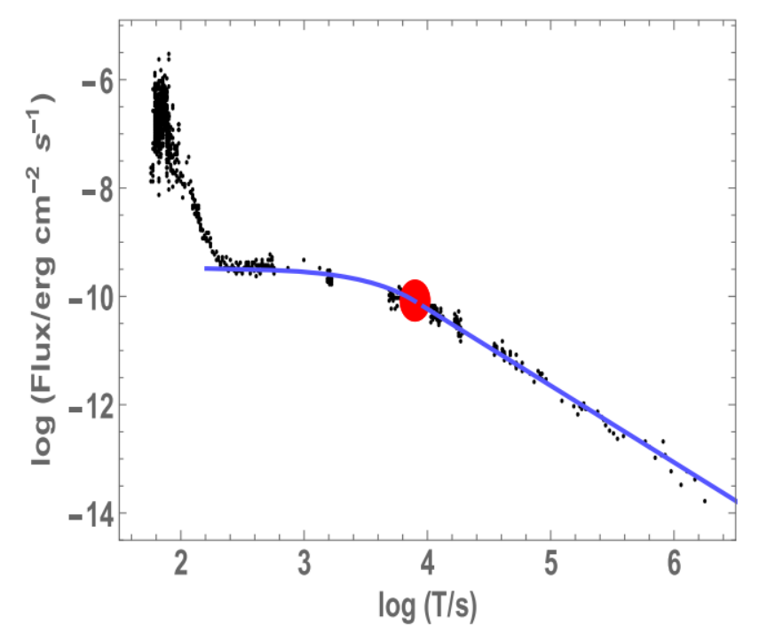
and denote the time in the X-ray at the end of the plateau and the same time, but in the optical wavelength respectively. are are their respective fluxes, while and are their respective luminosities. An approximation of the energy of the plateau is , see the left panel of Fig. 1.
- •
and are the peak time in the optical and the time since ejection of the pulse. and are their respective luminosities. is the respective flux of .
- •
is the peak time in the X-ray and and are its flux and luminosity respectively.
- •
and are the time at the end of the prompt emission within the W07 model and the time at which the flat and the step decay behaviours of the light curves join respectively.
- •
and are the times in which the 90% (between 5% and 95%) and 45% (between 5%-50%) of radiation is emitted in the prompt emission respectively.
- •
and are the differences in arrival time to the observer of the high energy photons and low energy photons and the shortest time over which the light curve increases by the of the peak flux of the pulse.
- •
, , , , and , , , , are the X-ray and optical luminosities at 200 s, at 10, 11, 12 hours and at 1 day respectively; , , , are the optical luminosity at 100 s, 1000 s, 10000 s and 7 hours; and are the isotropic prompt emission mean luminosity and the optical or X-ray luminosity of the late prompt emission at the time .
- •
, and , are the X-ray and optical fluxes at 11 hours and at 1 day respectively; , are the gamma-ray flux in the prompt and the X-ray flux in the afterglow respectively. and are their respective isotropic energies and and are the respective luminosities. indicates the prompt fluence in the gamma band correspondent to the rest frame isotropic prompt energy .
- •
, and are the optical isotropic energy in the afterglow phase, the total gamma isotropic energy and the prompt emission energy of the pulse.
- •
, and are the isotropic kinetic afterglow energy in X-ray, the prompt peak energy in the spectrum and the isotropic energy corrected for the beaming factor.
- •
, , , and are the X-ray temporal decay index in the afterglow phase, in the optical after s, in the X-ray after s and the optical or X-ray flat and steep temporal decay indices respectively.
- •
, and are the spectral index of the plateau emission in X-ray, the optical-to-X-ray spectral index for the end time of the plateau and the optical spectral index after s.
- •
, , , are the X-ray and optical frequencies, and the cooling and the peak frequencies of the synchrotron radiation.
All the time quantities described above are given in the observer frame, while with the upper index we denote in the text the observables in the GRB rest frame. The rest frame times are the observed times divided by the cosmic time expansion, for example, denotes the rest frame time at the end of the plateau emission.

In the following table we will give a list of the abbreviations/acronyms used through the text:
| Abbreviation | Meaning |
|---|---|
| DE | Dark Energy |
| EoS | Equation of State |
| CL | Confidence Level |
| IC | Intermediate Class GRB |
| SGRB | Short GRB |
| LGRB | Long GRBs |
| SGRBsEE | Short GRBs with extended emission |
| XRFs | X-ray Flashes |
| SNe | Supernovae |
| BH | Black Hole |
| z | redshift |
| FS | Forward Shock |
| RS | Reverse Shock |
| Hubble constant | |
| Matter density in CDM model | |
| Dark Energy density in CDM model | |
| curvature in CDM model | |
| error on the luminosity | |
| error on the time | |
| E4 | sample with |
| E0095 | sample with |
| W07 | Willingale et al. (2007) |
| Lorentz Factor | |
| Variability of the GRB light curve | |
| Hubble constant divided by 100 | |
| , | coefficients of the DE EoS |
| HD | Hubble Diagram |
| a | normalization of the relation |
| b | slope of the relation |
| intrinsic scatter of the relation | |
| intrinsic slope of the relation |
III The Afterglow Relations
Several relations appeared in literature relating only parameters in the afterglow, such as the relation [32] and similar ones in the optical and X-ray bands such as the unified - and - [54] and the - relations [102].
III.1 The Dainotti relation ( - )
The first relation to shed light on the plateau properties has been the -
one, hereafter also referred as LT. The phenomenon is an anti-relation between the X-ray luminosity
at the end of the plateau, , and the time in the X-ray at the end of the plateau, ,
for simplicity of notation we will refer to as .
It was discovered by [32] using
33 LGRBs detected by the Swift satellite in the X-ray energy band observed by XRT.
Among the 107 GRBs fitted by W07 phenomenological model, shown in the left panel of Fig. 1, only the GRBs that
have a good spectral
fitting of the plateau and firm determination of have been chosen. The functional form of the LT
relation obtained is the following:
| (1) |
with a normalization , a slope , an intrinsic scatter, and a Spearman correlation coefficient22 2 A computation of statistical dependence between two variables stating how good the relation between these variables can be represented employing a monotonic function. It assumes a value between and . . in the Swift XRT passband, keV, has been computed from the following equation:
| (2) |
where represents the GRB luminosity distance for a given , indicates the flux in the X-ray at the end of the plateau, and denotes the K-correction for cosmic expansion [13]. This anti-relation shows that the shorter the plateau duration, the more luminous the plateau. Since the ratio between the errors on both variables is close to unity, it means that both errors need to be considered and the Marquardt Levenberg algorithm is not the best fitting method to be applied in this circumstance. Therefore, a Bayesian approach [27] needs to be considered. This method takes into account the errors of both variables and an intrinsic scatter, , of unknown nature. However, the results of both the D’Agostini method and the Marquardt Levenberg algorithm are comparable. Due to the higher accuracy of the first method from now on the authors prefer this technique in their papers. Evidently, the tighter the relation, the better the chances to constrain the cosmological parameters. With this specific challenge in mind, a subsample of bursts has been chosen with particular selection criteria both on luminosity and time, namely and . After this selection has been applied, a subsample of 28 LGRBs was obtained with , thus reducing considerably the scatter.
In agreement with these results, through the analysis of the late prompt phase in optical and X-ray light curves
of 33 LGRBs,
also [54] found a common observational model for optical and X-ray light curves
with the same value for the slope, , obtained by [32]
when the time is limited between .
Instead, [33] from a sample of 62 LGRBs found , while for
the 8 IC GRBs pointed out a much steeper relation (). Finally, taking into
account the errors on luminosity () and time (), the
8 GRBs with the smallest errors were defined as the ones with .
For this subsample, [33] found a slope , see Fig. 2, the right panel of Fig.
3 and Table 2.
Similar to [33], also [10] and [134], with a sample of 64 and 14 LGRBs
respectively, found a slope , for details see Table 2.
Expanding the sample again to 77 LGRBs, [34] discovered a relation with .
Later, [85], considering in their sample of 50 LGRBs those GRBs with no visible plateau phase and employing
a broken power law as a fitting model, found a steeper slope ().
Thus, from all these analyses it is clear that a steepening of the slope has been
observed when the sample size is increased.
Therefore, before going further with additional analysis,
[36] decided to show how selection biases can influence the slope of the relation. They showed that
the steepening of the relation results from selection biases, while the intrinsic slope of the relation is
, see section V. Summarizing, [36] with a sample of
101 GRBs, confirmed the previous results from [33], as well as [125], with a data set
of 159 GRBs.


[38] also confirmed previous results of [36] but with a larger sample of 123 LGRBs. All the samples discussed are observed by SWIFT/XRT.
| Author | N | Type | Slope | Norm | Corr.coeff. | P |
|---|---|---|---|---|---|---|
| Dainotti et al. (2008) | 28 | 48.09 | -0.80 | |||
| Dainotti et al. (2008) | 33 | All GRBs | 48.54 | -0.74 | ||
| Cardone et al. (2009) | 28 | L | 48.09 | -0.74 | ||
| Ghisellini et al. (2009) | 33 | L | 48.09 | -0.74 | ||
| Cardone et al. (2010) | 66 | L | -0.68 | |||
| Dainotti et al. (2010) | 62 | L | -0.76 | |||
| Dainotti et al. (2010) | 8 | high luminosity | -0.93 | |||
| Dainotti et al. (2010) | 8 | IC | -0.66 | |||
| Dainotti et al. (2011a) | 77 | L | -0.69 | |||
| Sultana et al. (2012) | 14 | L | -0.88 | |||
| Bernardini et al. (2012) | 64 | L | 51.06 | -0.68 | ||
| Mangano et al. (2012) | 50 | L | -0.81 | |||
| Dainotti et al. (2013a) | 101 | ALL intrinsic | 52.94 | -0.74 | ||
| Dainotti et al. (2013b) | 101 | All GRBs | -0.74 | |||
| Dainotti et al. (2013b) | 101 | without short | 52.94 | -0.74 | ||
| Dainotti et al. (2013b) | 101 | simulated | -0.74 | |||
| Postnikov et al. (2014) | 101 | L () | -0.74 | |||
| Rowlinson et al. (2014) | 159 | intrinsic | 52.94 | -0.74 | ||
| Rowlinson et al. (2014) | 159 | observed | -0.74 | |||
| Rowlinson et al. (2014) | 159 | simulated | -0.74 | |||
| Dainotti et al (2015) | 123 | L | -0.74 | |||
| Dainotti et al. (2016c) | 19 | L-SNe | -0.83 |
In the context of reducing the scatter of the LT relation, [44] investigated the temporal decay indices
after the plateau phase for a sample of GRBs detected by Swift within two different models:
a simple power law, considering the decaying phase after the plateau phase, and the W07 one. It is pointed out that the results
are independent of the chosen model. It was checked if there are some common characteristics in GRBs phenomena that can
allow them to be used as standardizable candles like SNe Ia and to obtain some constraints revealing which is the best physical
interpretation describing the plateau emission.
The interesting result is that the LT relation for the low and high luminosity GRBs seems to depend differently on the
parameter, thus possibly implying a diverse density medium.
Continuing the search for a standard set of GRBs, [40] analyzed 176 GRB afterglow plateaus observed by
Swift with known redshifts which revealed that the subsample of LGRBs associated with SNe (LONG-SNe) presents a very
high correlation coefficient for the LT relation. They investigated the category of LONG GRBs associated
spectroscopically with SNe in order to compare the LT correlation for this sample with the one for LGRBs for which
no associated SN has been observed (hereafter LONG-NO-SNe, 128 GRBs). They checked if there is a difference among these
subsamples. They adopted first a non-parametric statistical method, the [46] one, to take into
account redshift evolution and check if and how this effect may steepen the slope for the
LONG-NO-SNe sample. This procedure is necessary due to the fact that this sample is observed at much higher redshift
than the GRB-SNe sample. Therefore, removing selection bias is the first step before any comparison among samples
observed at different redshifts could be properly performed. They have demonstrated that there is no evolution for the
slope of the LONG-NO-SNe sample and no evolution is expected for the LONG-SNe sample. The difference among the slopes
is statistically significant with the probability P=0.005 for LONG-SNe. This possibly suggests that the LONG-SNe with
firm spectroscopic features of the SNe associated might not require a standard energy reservoir in the plateau phase
unlike the LONG-NO-SNe. Therefore, this analysis may open new perspectives in future theoretical investigations of the
GRBs with plateau emission and associated with SNe. They also discuss how much this difference can be due to the jet
opening angle effect. The difference between the SNe-LONG (A+B) and LONG-NO-SNe sample is only statistically significant
at the 10% level when we consider the beaming correction. Thus, one can argue that the difference in slopes can be
partially due to the effect of the presence of low luminosity GRBs in the LONG-SNe sample that are not corrected for beaming.
However, the beaming corrections are not very accurate due to indeterminate jet opening angles, so the debate remains
open and it can only be resolved when we will gather more data.
In Table 2, we report a summary of the parameters and with and for the LT relation.
In conclusion, the most reliable parameters for this relation are those from
[36], because they have demonstrated that the intrinsic slope not affected by selection biases
is determined to be as computed through the Efron and Petrosian (EP) method.
III.1.1 Physical interpretation of the Dainotti relation ( - )
Here, we revise the theoretical interpretation of the LT relation, which is based mainly
on the accretion [18, 19] and the magnetar models [155, 41, 123, 124, 125].
The first one states that an accretion disc is created from the motion of
the material around the GRB progenitor star collapsing towards its progenitor core. After it is compressed by
the gravitational forces, the GRB emission takes place. For LGRBs, the early rate of decline in the initial steep
decay phase of the light curve
may provide information about the radial density distribution within the progenitor [71].
[18] predicted a steeper relation slope (-3/2) than the observed one
(), which on the other
hand is in good agreement with the prior emission model of [150].
Later, [19], using a sample of LGRBs and few SGRBs simulated the fall-back disks
surrounding the BH. They found that a circularization radius of the mass around the BH with value cm can give an
estimate for the plateau
duration of around s for LGRBs maintaining the initial fall back mass at solar masses (),
see the left panel
of Fig. 4. For SGRBs the radius is estimated to be cm.
The LT relation provides a lower limit for the accreting mass estimates to 33
3
This value can be
derived considering the total inferred accretion mass where c
is the light speed, f is the X-ray afterglow beaming factor, is the efficiency of the accretion onto the BH and
is the observed total energy of the plateau + later decay phases (the integral over time between and the end of afterglow,
see Eq. 2 of W07).. From their results, it was claimed that the LT relation could be obtained if a typical energy reservoir
in the fall-back mass is assumed, see the right panel of Fig. 4. However, in their analysis the very steep
initial decay following the prompt emission, which have been modelled by [80] as fall-back of the
progenitor core, is not considered.


Regarding the magnetar model, [155] studied the effects of an injecting central
engine on the GRB afterglow radiation, concentrating on a strongly magnetized millisecond pulsar.
For specific starting values of rotation period and magnetic field of the pulsar, the afterglow light curves should
exhibit an achromatic bump lasting from minutes to months, and the observation of such characteristics could
set some limits on the progenitor models.
More recently, [41] investigated the energy evolution in a relativistic
shock from a spinning down magnetar in spherical symmetry. With their fit of few observed Swift XRT light curves and
the parameters of this model, namely a spin period of ( ms), and high values of magnetic fields ( G),
they managed to well reproduce the properties of the shallow decay phase and the LT relation, see the left panel of
Fig. 5.
Afterward, [10] with a sample of 64 LGRBs confirmed, as previously founded by [41], that
the shallow decay phase of the GRB light curves and the LT relation can be well explained.
Then, [123] and [124] pointed out that energy injection is a fundamental mechanism
for describing the plateau emission of both LGRBs and SGRBs. In fact, the remnant of NS-NS mergers can form a magnetar,
and indeed
the origin of the majority of SGRBs is well explained through the energy injection by a magnetar.

Later, [125], using 159 GRBs from Swift catalogue, analytically demonstrated that the central engine model accounts for the LT relation assuming that the compact object is injecting energy into the forward shock (FS), a shock driven out into the surrounding circumstellar medium. The luminosity and plateau duration can be computed as follows:
| (3) |
and
| (4) |
where is in units of s, is in units of erg s-1, is the moment of inertia in units of g cm2, is the magnetic field strength at the poles in units of G, is the radius of the NS in units of cm and is the initial period of the compact object in milliseconds. Then, substituting the radius from eq. 4 into eq. 3, it was derived that:
| (5) |
Therefore, an intrinsic relation is confirmed directly from this formulation.
Although some magnetar plateaus are inconsistent with energy injection into the FS,
[125] showed that this emission is narrowly beamed
and has % efficiency in conversion of rotational energy from the compact object into the
observed plateau luminosity. In addition, the intrinsic LT relation slope, namely the one where
the selection biases are
appropriately removed, is explained within the spin-down of a newly formed magnetar at 1 level,
see right panel of Fig. 5.
The scatter in the relation is mainly due to the range of the initial spin periods.
After several papers discussing the origin of the LT relation within the context of the magnetar model,
very recently a debate has been opened by [118] on the reliability of this model as the correct
interpretation for the X-ray plateaus.
Using GRBs with known detected by Swift from its launch to August 2014, [118] concluded that the initial
magnetic field distribution,
used to interpret the GRB X-ray plateaus within the magnetar model does not match the features
of GRB-magnetars with the Galactic magnetar
population. Therefore, even though there are large uncertainties in these estimates due to GRB rates, metallicity and
star
formation, the GRB-magnetar model in its present
form is safe only if two kinds of magnetar progenitors are allowed. Namely, the GRB should be different from Galactic
magnetar ones
(for example for different metallicities) and should be considered supermagnetars (magnetars with an initial magnetic
field significantly large).
Finally, they set a limit of about on the number of stable magnetars produced in the Milky Way via a GRB in
the past Myr. However, it can be argued that since the rates of Galactic magnetars and GRBs are
really different, the number of Galactic magnetars cannot fully describe the origin of GRBs.
In fact the Galactic magnetar rate is likely to be greater than 10% than the core collapse SNe rate, while GRB rate is
much lower than that. In addition, the number of magnetars in the Milky Way may not be used as a constraint on the GRB
rate because the spin-down rates of GRB magnetars should be very rapid. Due to the low GRB rate it would not be easy to
detect these supermagnetars.
Thus, it can be claimed that no conflict stands among this paper and the previous ones.


Still in the context of the energy injection models, [141] found a relation between the optical flux at the end of the plateau and the time at the end of the plateau itself [106, 73] for which observed frame variables were considered. The range of all parameters describing the emission (, the fraction of the magnetic energy, , the initial density, ) is the principal cause of the scatter in the relation, but it does not affect the slope. Finally, it was claimed that both the wind (, where A is a constant) and the interstellar medium can reproduce the observed relation within both the reverse shock (RS, a shock driven back into the expanding bubble of the ejecta) and FS scenarios, see Fig. 6.


Considering alternative models explaining the LT relation, [135] studied the evolution of the Lorentz gamma factor, (where is the relative velocity between the inertial reference frames and is the light speed), during the whole duration of the light curves within the context of the Supercritical Pile Model. This model provides an explanation for both the steep-decline and the plateau or the steep-decline and the power law decay phase of the GRB afterglow, as observed in a large number of light curves, and for the LT relation. One of their most important results is that the duration of the plateau in the evolution of becomes shorter with a decreasing value of , where is the initial rest mass of the flow. This occurrence means that the more luminous the plateau, the shorter its duration and the smaller the , namely the energy.


Instead, in the context of the RS and FS emissions, [72], investigating the synchrotron radiation
in the thick shell scenario (i.e. when the RS is relativistic), found that this radiation
is compatible with the presence of the plateau phase, see the left panel of Fig. 7.
In addition, analyzing the -
relation in the framework of this model, they arrived at the conclusion that smooth energy injection
through the RS is favoured respect to the FS, see the right panel of Fig. 7.
[142], with a simulated sample of GRBs, found out that the observed LT relation
rules out basic thin shell models, but not basic thick ones. In fact, in the thick model, the
plateau phase comes from the late central
source activity or from additional kinetic energy transfer from slower ejecta
which catches up with the blast wave. As a drawback, in this
context, it is difficult to distinguish between FS and RS
emissions, or homogeneous and stellar wind-type environments.
In the thin shell case, the plateau phase is given by the pre-deceleration emission from a
slower component in a two-component or jet-type model, but this scenario is not in agreement with the observed LT
relation, see Fig. 8.
This, however, does not imply that acceptable fits using a thin shell model are not possible, but
further analysis is needed to exclude without any doubts thin shell models.
Another model which has not been tested yet on this correlation is the photospheric emission model
from stratified jets [60].
III.2 The unified - and - relations
In order to describe the unified picture of the X-ray and optical afterglow, it is necessary to introduce relevant
features regarding optical luminosities. To this end, [14] studied
the afterglow decay index in 8 GRBs in both X-ray and optical wavelengths. In the X-ray, the brightest GRBs had decay
indices around and the dimmest GRBs had decay indices around .
Instead, they didn’t observe this trend for the optical light curves,
probably due to the host galaxy absorption.
Later, [95] discovered that the
monochromatic optical luminosities at 12 hours, , of 24 LGRBs cluster at
erg s-1 Hz-1,
with . The distribution of is less scattered
than the one of , the luminosity at 12 hours in the X-ray, and the one of the
ratio , where is the rest frame isotropic prompt
energy. Three bursts are outliers because they have luminosity which is smaller by a
factor . This result suggests the existence of a family of intrinsically optically underluminous dark
GRBs, namely GRBs where the optical-to-X-ray
spectral index, , is shallower than the X-ray spectral index minus 0.5, .
[75] confirmed these results.
They found a bimodal distribution of using 44 GRBs.
[96] also confirmed these findings. They
analyzed selection effects present in their observations extending
the sample to 55 LGRBs
with known and rest-frame optical extinction detected by the Swift satellite.
In contrast, [90], [101], [153] and [91] found no bimodality in
the distributions of , and , investigating samples
of 44, 24, 40 and 47 GRBs respectively.
Instead, with the aim of finding a unifying representation of the GRB afterglow phase,
[54] fitted the light curves assuming this functional form:
| (6) |
They used a data sample of 33 LGRBs detected by Swift in X-ray (0.3-10 keV) and optical R bands (see the left and middle panels of Fig. 9). Within this approximation, the agreement with data is reasonably good, and they confirmed the X-ray LT relation.


Through their analysis using a data sample of 32 Swift GRBs, [78] found that the
optical peak luminosity, , in the R band
in units of erg s-1 and the optical peak time, , are anti-correlated, see
the right panel of Fig. 9, with a slope and .
They deduced that a fainter bump has its maximum later than brighter ones and it also presents a
longer duration.
[106] showed a similar relation to the one presented in [78].
They found a anti-relation using 37 Swift GRBs.
This result may indicate a unique mechanism for the optical
afterglow even though the optical energy has a quite large scatter.
Afterwards, [73] found a relation (see the left panel of Fig. 10) similar to the LT relation, but in the R band. They used 39 GRBs with optical data available in the literature. This relation is between the optical luminosity at the end of the plateau, , in units of erg s-1 and the optical end of the plateau time, , in the shallow decay phase of the GRB light curves, denoted with the index S. They found a slope , and .
| Correlations | Author | N | Slope | Corr.coeff. | P |
|---|---|---|---|---|---|
| Liang et al. (2010) | 32 | -0.90 | |||
| Panaitescu & Vestrand (2011) | 37 | ||||
| - | Li et al. (2012) | 39 |
varies from to erg s-1, and in some GRBs with an early break reaches erg s-1, see the middle panel of Fig. 10. spans from tens of seconds to several days after the GRB trigger, with a typical shallow peak time of seconds, see the right panel of Fig. 10. By plotting in units of erg s-1 as a function of in the burst frame, they observed that optical data have a similar trend to the X-ray data. In fact, this power law relation, presented in the left panel of Fig. 10, with an index of is similar to that derived for the X-ray flares (see sec. IV.6). XRF phenomena are described in sec. 1. As a consequence, they recovered the LT relation. In Table 3 a summary of the relations described in this section is displayed.
III.2.1 Physical interpretation of the unified - and - relations
In the unified - and - relations
[54] considered the flux as the sum of synchrotron radiation caused by
the standard FS due to the fireball impacting the
circumburst medium and of another component may be produced by a long-lived central engine, which resembles mechanisms
attributed to a “late prompt”.
Even if based in part on a phenomenological model, [54] explained situations in which achromatic and
chromatic
jet break are either present or not in the observed light curves.
In addition, from their analysis, the decay slope of the late prompt emission results to be
(see blue dashed line for X-ray and optical emission
in the left and middle panels of Fig. 9 respectively), really close within the errors
to the value of the temporal accretion rate
of fall-back material (i.e. ,
see red dashed line for X-ray and for optical emission in the left and middle panels of
Fig. 9 respectively). This explains the activity of the central engine for such a long duration.
For a similar interpretation within the context of the accretion onto the BH related to LT relation
see sec. III.1.1.
[78] claimed that the external shock model explains well the anti-relation between
and , because later deceleration time is equivalent to slower ejecta and thus to a less
luminous emission.
Furthermore, [105] from the analysis of the relation explained the peaky
afterglows (those with ) as being a bit outside the cone of view, while the plateau as
off-axis events and due to the angular structure of the jet.
Later, [106] asserted that
the double-jet structure of the ejecta is problematic. To overcome this issue, they suggested a
model in which both the peaky and plateau afterglows depend on how much time the central engine allows for the energy
injection.
More specifically, impulsive ejecta with a narrow range of are responsible for the peaky afterglows, while the plateau
afterglows are produced by a distribution of initial which keeps the energy injection till s.
Later, [73] pointed out that late
GRB central engine activities can account for both optical flares
and the optical shallow-decay segments. These activities
can be either erratic (for flares) or steady (for internal plateaus).
A normal decay follows the external plateaus with typically around , thus possibly originated by an
external shock with the shallow decay segment
caused by continuous energy injection into the blast wave [119, 28, 129, 155]. Instead, the internal
plateaus, found first by [137] in GRB 070110 and later studied statistically by [77], are
followed by a much steeper decay ( steeper than -3), which
needs to be powered by internal dissipation of a late outflow. In summary, the afterglow can be interpreted as a mix
of internal and external components.
III.3 The - relation and its physical interpretation
[102] discovered a relation between the optical luminosity at 200 s, , and the optical temporal decay index after 200 s, , see the right panel of Fig. 11. They used a sample of 48 LGRB afterglow light curves at Å detected by UVOT on board of the Swift satellite, see the left panel of Fig. 11. The best fit line for this relation is given by:
| (7) |
with and a significance of 99.998% (4.2 ).
This relation means that the brightest GRBs decay faster than the dimmest ones. To obtain
the light curves employed for building the relation, they used the criteria
from [101] in order to guarantee that the entire UVOT light curve is not noisy,
namely with a high signal to noise (S/N) ratio: the optical/UV light curves must
be observed in the V filter of the UVOT with a magnitude , UVOT observations must
have begun within the first 400 s after the BAT trigger and the afterglow must have been observed until at
least s after the trigger.
Their results pointed out the dependence of this relation is on the differences in the observing angle and on
the rate of the energy release from the central engine.
As a further step, [103], using the same data set, investigated the same
relation both in optical and in X-ray wavelengths in order to make a comparison, and they confirmed previous
optical results finding a similar slope for both relations.
In addition, they analyzed the connection between
the temporal decay indices after s (in X-ray and optical) obtaining as best fit relation
, see the left panel of Fig. 12.
They yielded some similarities between optical and
X-ray components of GRBs from these studies. Their results were in disagreement
with those previously found by [139], who investigated the relation between the optical and X-ray temporal
decay
indices in the normal decay phase derived from the external shock model.
In fact, a good fraction of outliers was found in this previous work.
[117] studied a similar relation using 237 Swift LGRBs,
but in X-ray. For this relation, it was found that slope and solid evidence
for a strong connection between optical and X-ray components of GRBs was discovered as well.
In conclusion, the Monte Carlo simulations and the statistical tests validated
the relation between and
by [102]. In addition,
it shows a possible connection with its equivalent,
the LT relation in X-ray, implying a common physical mechanism.
In Table 4 a summary of the relations described in this section is reported.


Regarding the physical interpretation of the - relation, [102] explored several scenarios. The first one implies that the relation can be due to the interaction of the jet with the external medium. In a straightforward scenario is not a fixed value and all optical afterglows stem from only one closure relation where and are related linearly. Thus a relation between and should naturally appear. Contrary to this expectation, and are poorly correlated, see the right panel of Fig. 12, and there is no evidence for the existence of a relation between and . Therefore, this scenario cannot be ascribed as the cause of the - relation.


In the second scenario, they assumed that the -
relation is produced by few closure relations indicated by lines in the right panel of Fig. 12.
However, from this picture, the and values with similar luminosities do not gather around a particular
closure relation, thus also the basic standard model is not a good explanation of the
relation.
As a conclusion, the afterglow model is more complex than it was
considered in the past. It is highly likely that there are physical properties that control the emission mechanism and the decay
rate in the afterglow that still need to be investigated.
Therefore, [102] proposed two additional alternatives.
The first is related to some properties of the central engine
influencing the rate of energy release so that for fainter
afterglows, the energy is released more slowly. Otherwise, the relation can be due to different observing angles where
observers at smaller viewing angles see brighter and faster decaying light curves.
| Correlations | Author | N | Slope | Norm | Corr.coeff. | P |
|---|---|---|---|---|---|---|
| - | Oates et al. (2012) | 48 | ||||
| Oates et al. (2015) | 48 | |||||
| - | Racusin et al. (2016) | 237 |
As pointed out by [36], the - relation is related to the LT one since both show an anti-relation between luminosity and decay rate of the light curve or time. The key point would be to understand how they relate to each other and the possible common physics that eventually drives both of them. To this end, [103] compared the observed relations with the ones obtained with the simulated sample. The luminosity-decay relationship in the optical/UV is in agreement with that in the X-ray, inferring a common mechanism.
IV The Prompt-Afterglow Relations
As we have discussed in the previous paragraphs, the nature of the plateau and the relations (e.g. the optical one) based on similar physics and directly related to the plateau are still under investigation. For this reason, several models have been proposed. To further enhance its theoretical understanding, it is necessary to evaluate the connection between plateaus and prompt phases. To this end, we hereby review the prompt-afterglow relations, thus helping to establish a more complete picture of the plateau GRB phenomenon.
IV.1 The relation and its physical interpretation
W07 analyzed the relation between the gamma flux in the prompt phase, , and the X-ray flux in the afterglow, using 107 Swift GRBs, see the upper left panel of Fig. 13. They calculated in the XRT band (0.3-10 keV), while in the BAT (15-150 keV) plus the XRT (0.3-10 keV) energy band. For GRBs with known redshift, as shown in the upper right panel of Fig. 13, they investigated the prompt isotropic energy, , and the afterglow isotropic energy, , assuming a cosmology with km s-1 Mpc-1, and .


At the same time, [77] focused on the relation between
and using a sample of 53 LGRBs. They pointed out a good relation with
, see the bottom left panel of Fig. 13.
In agreement with these results, [78] and [106] analyzed this relation,
using respectively 32 and 37 GRBs, but considering energy bands different from that used in [77];
they obtained the slopes and respectively (see the left and middle panels of Fig. 14).


[124] and [56] confirmed these results, see the left and middle panels of Fig.
15. In fact, they obtained a relation with slope
using 43 SGRBs and 232 GRBs with spectroscopic redshifts detected by Swift respectively.
Finally, [38] analyzed this relation to find some constraints on the ratio of
to , considering a sample of 123 LGRBs, see the right panel of Fig. 15.
Instead, [54], with a sample of 33 LGRBs, considered a similar relation, but assuming the X-ray plateau
energy, , as an estimation of , see the bottom right panel of Fig. 13; they found
a slope .
In addition, [54] also investigated the relation between
and the kinetic isotropic energy in the afterglow, , with the same sample,
finding a relation with .
Similarly, [116] studied the same relation, using 69 GRBs and assuming different efficiencies to find some
limits between and , see the right panel of Fig. 14.
This relation was most likely used to study the differences in detection
of several instruments and to analyze the transferring process of kinetic energy into the prompt emission in GRBs,
making the relation by [116] the most reliable one.
To summarize, for comparing the energies in the prompt and the afterglow phases,
a relation was studied by [77] and
confirmed by [124], [56] and [38]. The last study found also some limitations
on the ratio among the prompt and the afterglow energies. Furthermore, instead of ,
was considered for the investigation, although this quantity provided similar results to the previous ones
[54]. Finally, the relation between
and was studied by [54] and confirmed by [116], who examined
the energy transfer in the prompt phase. These relations are relevant because of their usefulness for investigating
the efficiency of the emission processes during the transition from the prompt phase to the afterglow one, and for
explaining which the connection between these two emission phases is. As a main result, [54]
and [116] claimed that the fraction of kinetic energy transferred from the prompt phase to the afterglow one
is around 10%. In particular, [116] yielded that this value of the transferred kinetic
energy, for BAT-detected GRBs, is in agreement with the analysis by [157] for which the internal shock model
well describes this value in the case of a late energy transfer from the fireball to the surrounding medium
[154].
In Table 5, a summary of the relations described in this section is presented.
As regards the physical interpretation of the relation,
[116], estimating the efficiency parameter for the BAT sample, confirmed
the [157] result for which of BAT bursts have .
However, for the samples from the Gamma Burst Monitor (GBM)
and the Large Area Telescope (LAT), on board the Fermi satellite44
4
The Fermi Gamma ray
Space Telescope (FGST), launched in 2008 and still running, is a space observatory being
used to perform gamma ray astronomy observations from low Earth orbit. Its main instrument is the Large Area Telescope (LAT), an
imaging gamma ray detector, (a pair-conversion instrument) which detects photons with energy from about 20 MeV to 300 GeV with a
field of view of about 20% of the sky; it is a sequel to the EGRET instrument on the Compton gamma ray observatory (CGRO). Another
instrument aboard Fermi is the Gamma Ray Burst Monitor (GBM), which is used to study prompt GRBs from keV to MeV.,
they found that only 25% of the GBM bursts and none of the LAT bursts have
. This implies that Fermi GRBs are more efficient at transferring kinetic energy
into prompt radiation.


| Correlations | Author | N | Slope | Norm | Corr.coeff. | P |
|---|---|---|---|---|---|---|
| Liang et al. (2007) | 53 | 0.79 | ||||
| Liang et al. (2010) | 32 | 0.82 | ||||
| Panaitescu & Vestrand (2011) | 37 | 1.18 | 0.66 | |||
| Ghisellini et al. (2009) | 33 | 0.86 | ||||
| Ghisellini et al. (2009) | 33 | 0.42 |
IV.2 The relation and its physical interpretation
[6] investigated the prompt and afterglow energies in the observed frame of 16 SGRBs. A large fraction of them (80%) follows a linear relation between the prompt fluence in the gamma band, , in the BAT range and the X-ray flux at 1 day, , in the XRT band given by:
| (8) |
with and . [49] confirmed his results investigating the same relation, but with X-ray fluxes at 11 hours, , see Fig. 16.

Later, [100] considered the relation between or the optical flux at 11 hours, ,
and , finding an almost linear relation, see Fig. 17. They used a data set
of 37 SGRBs and 421 LGRBs detected by Swift.
[106] confirmed, in part, these results. They found a similar relation between
and using 37 GRBs, but with a higher slope (), see the left panel of Fig.
18.
[62] showed a linear relation , where is the X-ray
luminosity at 10 hours calculated in the
2-10 keV energy range, while in the 20-2000 keV energy range, see the left panel of
Fig. 19.
This relation compares four long events spectroscopically associated with SNe with “regular” energetic LGRBs
( erg). The results possibly indicate a common
efficiency for transforming kinetic energy into gamma rays
in the prompt phase for both these four events and for “regular” energetic LGRBs.
The same relation has been studied in the context of the low luminosity versus normal luminosity GRBs.
Indeed, [3] found that the relation between , in the 2-10 keV band,
and , in the 1-10000 keV band, becomes stronger () including sub-energetic GRBs
as GRB 060218, GRB 980425
and GRB 031203, see the middle panel of Fig. 19. Therefore, it is claimed
that sub-energetic GRBs are intrinsically faint and are considered to some extent normal cosmological GRBs.
Finally, [6] also analyzed the relation between the X-ray luminosity at one day,
, and , using 13 SGRBs with measured . They found a slope
(see the right panel of Fig. 18).


[78] confirmed his results in the optical range using a sample of 32 Swift GRBs ( with , see the right panel of Fig. 19). In addition, [63] also confirmed his results with a sample of 76 LGRBs ( with , see the left panel of Fig. 20).


Similarly, [35] analyzed the relation between
and
using the light curves of 66 LGRBs from the Swift BAT+XRT repository, http://www.swift.
ac.uk/burst-analyser/.
Their sample has been divided into two subsamples: E4 formed of 62 LGRBs and E0095 consisting of 8 LGRBs, assuming
as a parameter representing the goodness of the fit.
For the E4 subsample it was found:
| (9) |
with and , while for the E0095 subsample
| (10) |
with and .
Thus, it was concluded that the small error energy sample led to a higher relation
and to the existence of a subset of GRBs which can yield a “standardizable candle”.
Furthermore, since and are strongly correlated, and the slope is roughly -1, the energy
reservoir of the plateau is roughly constant. Since and are both linked with
,
then the relation is straightforward.
For its modification
taking into account of the whole X-ray light curves see [11].
As further confirmations of the relation, [42] and [87]
found a relation between and with slope and ,
using 58 and 297 Swift LGRBs respectively.
Furthermore, [7] studied the relation between the X-ray luminosities at 11 hours, , and , and the relation between
the optical luminosity at 7 hours and for a sample of 70 SGRBs
and 73 LGRBs detected mostly by Swift. He found that the observed relations are flatter
than the ones simulated by [63], see the middle and right panels of Fig. 20.
Regarding the relation between and the optical luminosities, [103] analyzed the relation
between or and with a sample of 48 LGRBs. They claimed
a strong connection between prompt and afterglow phases, see Fig. 21 and Table 6. This relation permits to
study some important spectral characteristics of GRBs, the optical and X-ray components of the radiation process and
the standard afterglow model. In Table 6, a summary of the relations described in this section is shown.
Regarding the physical interpretation of the relation,
[49] underlined that the optical
and X-ray radiation are characterized by . This value matches the slow cooling case,
important at 11 hours, when the electron distribution power law index is for .
[103] pointed out that within the standard afterglow model, the
relations are expected.
However, the slopes of the simulated and observed relations are inconsistent at 3 due to values set for the
parameter. If the distribution of the efficiencies is not sufficiently narrow the relation will be more disperse. Thus, the
simulations repeated with and gave, anyway, incompatible results between the simulated and observed slopes at
3 .
| Correlations | Author | N | Slope | Norm | Corr.coeff. | P |
| Berger (2007) | 16 | 0.86 | ||||
| Gehrels et al. (2008) | 111 | 0.53 | ||||
| Gehrels et al. (2008) | 10 | 0.35 | 0.31 | |||
| Nysewander et al. (2009) | 421 | |||||
| Nysewander et al. (2009) | 37 | |||||
| Nysewander et al. (2009) | 421 | |||||
| Nysewander et al. (2009) | 37 | |||||
| Panaitescu&Vestrand (2011) | 37 | 1.67 | 0.75 | |||
| Berger (2007) | 13 | 0.94 | ||||
| Liang et al. (2010) | 32 | 0.87 | ||||
| Kann et al. (2010) | 76 | 0.36 | ||||
| Dainotti et al. (2011b) | 62 | 0.43 | ||||
| Dainotti et al. (2011b) | 8 | 0.83 | ||||
| D’Avanzo et al. (2012) | 58 | |||||
| Margutti et al. (2013) | 297 | |||||
| Berger (2014) | 73 | 0.72 | 44.75 | |||
| Berger (2014) | 70 | 0.83 | 43.93 | |||
| Berger (2014) | 73 | 0.73 | 43.70 | |||
| Berger (2014) | 70 | 0.74 | 42.84 | |||
| Oates et al. (2015) | 48 | 0.83 | ||||
| Oates et al. (2015) | 48 | 0.76 |
IV.3 The relation and its physical interpretation
In the observed frame, [61] studied the versus distribution, in the optical R band and in the keV band respectively, using all known GRBs with a detected X-ray afterglow, see the left panel of Fig. 22. Different from the previous definition of dark bursts (where dark bursts were simply defined as those bursts in which the optical transient is not observed), they defined these bursts as GRBs where the optical-to-X-ray spectral index, , is shallower than the X-ray spectral index minus 0.5, . They found out 5 dark bursts among 52 observed by Beppo-SAX55 5 Beppo-SAX, (1996-2003), was an Italian-Dutch satellite capable of simultaneously observing targets over more than 3 decades of energy, from to keV with relatively large area, good (for that time) energy resolution and imaging capabilities (with a spatial resolution of arcminute between and keV). The instruments on board Beppo-SAX are Low Energy Concentrator Spectrometer (LECS), Medium Energy Concentrator Spectrometer (MECS), High Pressure Gas Scintillation Proportional Counter (HPGSPC), Phoswich Detector System (PDS) and Wide Field Camera (WFC, from keV and from keV). The first four instruments point to the same direction allowing observations in the broad energy range (0.1-300 keV). With the WFC it was possible to model the afterglow as a simple power law, mainly due to the lack of observations during a certain period in the GRB light curve.. This analysis aimed at distinguishing dark GRBs through Swift. [50] and [49] confirmed the results using a data sample of 19 SGRBs and 37 LGRBs6 SGRBs respectively, see the middle and right panels of Fig. 22. In particular, [49] obtained a slope for LGRBs and for SGRBs.


Instead in the rest-rest frame, [7] studied the relation between and on 70 SGRBs
and 73 LGRBs, finding some similarities between SGRBs and LGRBs and a central value
, see the left panel of Fig. 23.
[103] improved their study. They analyzed a similar relation with a sample of 48 LGRBs,
but using and , see the right panel of Fig. 23.
The slope obtained has a value .
This relation helps to explore the synchrotron spectrum of GRBs and to obtain some constraints on the circumburst
medium for both LGRBs and SGRBs. In Table 7 a summary of the relations
described in this section is displayed.


| Correlations | Author | N | Slope | Norm | Corr.coeff. | P |
| Gehrels et al. (2008) | 6 | |||||
| 37 | ||||||
| Berger (2014) | 70 | 0.08 | ||||
| 73 | 0.08 | |||||
| Oates et al. (2015) | 48 | 0.81 |
Regarding the physical interpretation of the relation, [7] showed that, in the context of the synchrotron model, the comparison of and indicated that usually is near or higher than the X-ray band. Indeed, LGRBs have often greater circumburst medium densities (about times greater than SGRBs) and therefore .
IV.4 The relation
In [35] the connections between the physical properties of the prompt emission and were analyzed using a sample of 62 Swift LGRBs. A relation was found between in the XRT band and the isotropic prompt luminosity, , in the BAT energy band, see the left panel of Fig. 24. This relationship can be fitted with the following equation:
| (11) |
obtaining and .
In this paper was related to several prompt luminosities defined using different time scales,
such as , (the time in which the
45% between 5%-50% of radiation is emitted in the prompt emission), and (the time at
the end of the prompt emission within the W07 model).
Furthermore, the E4 (defined in Table 1) subsample of LGRBs with known from a sample of
77 Swift LGRBs and the E0095 subsample of 8 GRBs with smooth light curves were used, see black and
red points in the left panel of Fig. 24.
Therefore, it has been shown that the GRB subsample with the strongest correlation coefficient
for the LT relation also implies the tightest prompt-afterglow relations.
This subsample can be used as a standard one for astrophysical and cosmological studies.
In the middle panel of Fig. 24, the correlation coefficients are shown for the following distributions: , represented by different colours,
namely red, black, green and blue respectively.
No significant relations for the IC bursts have been found out. However, the paucity of the data does not allow a
definitive statement.
From this analysis, it is clear that the inclusion of the IC GRB class does not strengthen the existing relations.
| E4 | E0095 | |||
| Correlations | (b, a) | (b, a) | ||
| P | P | |||
| 0.59 | 0.95 | |||
| 0.62 | 0.90 | |||
| 0.60 | 0.93 | |||
| 0.62 | 0.94 | |||
| 0.46 | 0.95 | |||
| 0.56 | 0.90 | |||
| 0.43 | 0.83 | |||
| 0.52 | 0.75 | |||
| -0.19 | -0.81 | |||
| -0.21 | -0.69 | |||
| 0.54 | ||||
| 0.51 | 0.80 | |||
| -0.36 | -0.74 | |||
| -0.35 | -0.77 | |||
| 0.81 | 0.76 | |||
| 0.67 | 0.92 | |||
In general, this study pointed out that the plateau phase results connected to the inner engine. In addition, also relations between and several other prompt emission parameters were analyzed, including and the variability, . As a result, relevant relations are found between these quantities, except for the variability parameter, see Table 8.


IV.5 The relation
[38] further investigated the prompt-afterglow relations presenting an updated analysis of 123 Swift BAT+XRT light curves of LGRBs with known and afterglow plateau phase. The relation between the peak luminosity of the prompt phase in the X-ray, , and can be written as follows:
| (12) |
with , and with and , see the left panel of Fig. 25. In the literature is denoted as:
| (13) |


The relation [35] for the same GRB sample presented a correlation coefficient, , smaller than the one of the relation, see sec. IV.4. This implied that a better definition of the luminosity or energy parameters improves by 24%. In the left panel of Fig. 25 is calculated directly from the peak flux in X-ray, , considering a broken or a simple power law as the best fit of the spectral model. Thus, the error propagation due to time and energy is not involved, differently from the earlier considered luminosities. In addition, [38] preferred the to the relations presented in [35], namely the , due to the fact that and can undergo double bias truncation due to high and low energy detector threshold. Instead, this problem does not appear for [81]. Furthermore, to show that the relation is robust, the redshift dependence induced by the distance luminosity was eliminated employing fluxes rather than luminosities. A relation between and was obtained with , see the right panel of Fig. 25.


However, for further details about a quantitative analysis of the selection effects see sec.
V.
Finally, [38] showed that the LT relation has a different slope,
at more than 2 , from the one of the prompt phase relation between the
time since ejection of the pulse and the respective luminosity,
[149], see the left panel of
Fig. 26.
This difference also implied a discrepancy in the distributions of the energy and time, see the right panel of
Fig. 26.
The interpretation of this discrepancy between the slopes opens a new perspective in the theoretical understanding of
these observational facts, see the next section for details.
As a further step, [30] analyzed this relation
adding as a third parameter with a sample of 122 LGRBs (without XRFs and GRBs associated to SNe). They found
a tight relation:
| (14) |
with , , and . Additionally, the scatter could be further reduced considering the subsample of 40 LGRBs having light curves with good data coverage and flat plateaus:
| (15) |
with , , and . These results may suggest the use of this plane as a “fundamental” plane for GRBs and for further cosmological studies.
IV.5.1 Physical interpretation of the and the relations
In [38], the two distinct slopes of the luminosity-duration and the energy-duration distributions of prompt and plateau pulses could reveal that these two are different characteristics of the radiation: the former may be generated by internal shocks and the latter by the external shocks. Indeed, if the plateau is produced by synchrotron radiation from the external shock, then all the pulses have analogous physical conditions (e.g. the power law index of the electron distribution). In addition, the prompt-afterglow connections were analyzed in order to better explain the existing physical models of GRB emission predicting the and the relations together with the LT one in the prompt and afterglow phases. They claimed that the model better explaining these relationships is the one by [58]. In this work they considered two scenarios: one in the standard FS model assuming a modification of the microphysics parameters to decrease the efficiency at initial stages of the GRB evolution; in the latter the early afterglow stems from a long-lived RS in the FS scenario. In the FS scenario a wind external medium is assumed together with a microphysics parameter , the amount of the internal energy going into electrons (or positrons), where n is the density medium. In the case of is possible to reproduce a flat plateau. Thus, even operating on just one parameter can lead to the formation of a plateau that also reproduces the and the relations. Alternatively, in the RS scenario, in order to obtain the observed prompt-afterglow relationships, the typical of the ejecta should rise with the burst energy.

In addition, [126] pointed out that the induced gravitational collapse paradigm
can recover the and the relations. This model
considers the very energetic ( erg) LGRBs for which the SNe has been seen.
The light curves were built assuming for the external medium either a radial structure for the wind
[57, 8, 9, 16] or a partition of the
shell [31], therefore well matching the afterglow plateau and the prompt emission.
Recently, [64] within the context of the Supercritical Pile GRB Model claimed that they can reproduce
the
and the relations, because the ratio, R, between the luminosities appears consistent with the
one between the mean prompt energy flux from BAT and the afterglow plateau fluxes detected by XRT. In particular,
is close to the proton to electron mass ratio, see Fig. 27.
Indeed, this is a new challenge for theoretical modelling that would need to consider, simultaneously, the several
prompt-afterglow connections in order to better reproduce the phenomenology of the relations from a statistical point of view.
IV.6 The relation and its physical interpretation
[78] studied the relation between the width of the light curve flares, , and of the flares, denoted with the index F, using a sample of 32 Swift GRBs, see the left panel of Fig. 28. This relation reads as follows:
| (16) |
with .


Later, [73] found the same relation as [78], but with smaller values of normalization and slope, using 24 flares from 19 single-pulse GRBs observed with CGRO/BATSE66 6 Among the instruments of the Compton Gamma Ray Observatory (CGRO) satellite, running from 1991 to 2001, the Burst and Transient Source Experiment (BATSE) played a fundamental role in the measurements of GRB spectral features in the range from keV to MeV. Bursts were typically detected at rates of roughly one per day over the 9-year CGRO mission within a time interval ranging from s up to about s. Therefore, this satellite enabled careful analysis of the spectral properties of the GRB prompt emission., see the right panel of Fig. 28. However, for these 19 GRBs only in 14 GRBs a flare activity is distinctly visible. The relationship was given by:
| (17) |
They claimed that earlier flares are brighter and narrower than later ones.
They compared the distribution for the
X-ray flares detected by Swift/XRT with the one for the
optical flares in the R band. As a conclusion, they seemed to have a similar behaviour
[25, 86], see the right panel of Fig. 28.
Furthermore, in the rest frame band, they found a relation between the
of the flares in the R energy in units of erg s-1 and of the flares
using 19 GRBs, see Fig. 29.
Both prompt pulses and X-ray and optical flares are correlated and present a visible temporal evolution, as seen in
Fig. 29. This relation is given by:
| (18) |
with and . spans from tens of seconds to seconds, instead the varies from to erg s-1, with an average value of erg s-1. In addition, considering only the most luminous GRBs, they found that was strongly anti-correlated to in the keV energy band:
| (19) |
with . These outcomes revealed that the GRB flares in the optical wavelength with higher peak earlier and are much more luminous. In Table 9 a summary of the relations described in this section is displayed.
| Correlations | Author | N | Slope | Norm | Corr.coeff. | P |
|---|---|---|---|---|---|---|
| Liang et al. (2010) | 32 | 0.94 | ||||
| Li et al. (2012) | 19 | 1.01 | -0.32 | |||
| Li et al. (2012) | 19 | 0.85 | ||||
| Li et al. (2012) | 19 | 0.92 |
As regards the physical interpretation of the relationship, [73] found that the flares are separated components superimposed to the afterglow phase. The coupling between and suggested that the prompt -ray and late optical flare emission may arise from the same mechanism, namely from a central engine that can periodically eject a number of shells during the emission. Impacts of these shells could create internal shocks or magnetic turbulent reconnections, which would emerge from the variability [67, 156]. [47] revealed no relevant pattern in the width and intensity distributions using gamma ray data only. In addition, the usual tendency of the relation cannot be due to hydrodynamical diffusion of the shells emitted at recent times, but it is necessary that the central engine radiates thicker and fainter shells at late stages [88]. This could be explained as flares generated by clumps, such that the diffusion during the accretion mechanism would extend the accretion duration onto the BH [108, 115].
V Selection Effects
Selection effects are distortions or biases that usually occur when the sample observed is not representative of the
“true” population itself. This kind of biases usually affects GRB relations.
[46], [81], [36, 29] and [111] emphasized that when
dealing with a multivariate data set, it is imperative to determine first the true
relations among the variables, not those introduced by the observational selection effects,
before obtaining the individual distributions of the variables themselves.
This study is needed for claiming the existence of the intrinsic relations. A relation can be called
intrinsic only if it is carefully tested and corrected for these biases.
The selection effects present in the relations discussed above are mostly due to the dependence of
the parameters on the redshift,
like in the case of the time and the luminosity evolution, or due to the threshold of the detector used.
In this section, we describe several different methods to deal with selection biases.
In paragraph V.1, we discuss the redshift induced relation
through a qualitative method, while in V.2 we present a more quantitative approach through the EP method.
In V.3, we describe how to obtain the intrinsic relations corrected by selection biases, and
in V.4 we report the selection effects for the optical and X-ray luminosities. Lastly, in V.5
we show the evaluation of the intrinsic relation through Monte Carlo simulations.
V.1 Redshift induced relations
An important source of possible selection effects is the dependence of the variables on the redshift. To this end, [34] investigated the redshift evolution of the parameters of the LT relation, because a change of the relation slope has been observed when comparing several analyses [32, 33]. Namely, in the first paper, it was found and in the latter . Therefore, it became crucial to understand the reason of this change, even if the two slopes are still comparable at the 1- level. The distribution of the 62 LGRBs in the sample is not uniform within the range with few data points at large redshifts. Even if this sample is sparse, it was important to investigate whether the calibration coefficients were in agreement within the error bars over this large redshift interval, see the left panel of Fig. 30.
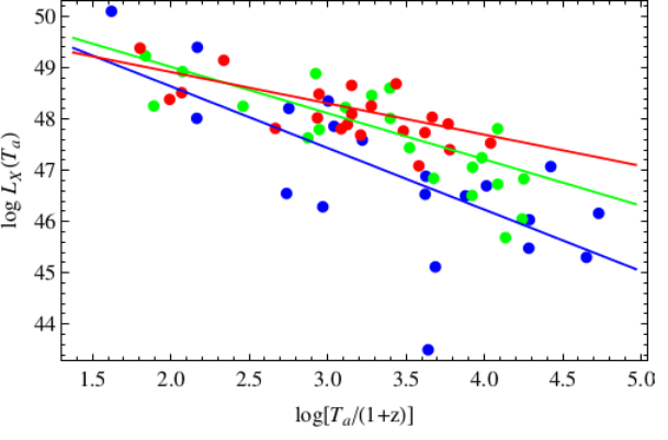

For this reason, the data set was separated in three redshift bins with the same number of elements, , and presented as blue, green and red points respectively in the left panel of Fig. 30. The results are presented in Table 10.
| Id | ||||
|---|---|---|---|---|
| Z1 | -0.69 | (-1.20, 51.04, 0.98) | ||
| Z2 | -0.83 | (-0.90, 50.82, 0.43) | ||
| Z3 | -0.63 | (-0.61, 50.14, 0.26) |
The correlation coefficient was found quite high in each redshift bins, supporting the
independence of the LT relation on . The slopes for
bins and are comparable within the CL, while the slopes in bins and only
within the CL, see Table 10. On the contrary, the normalization is comparable in all the bins.
From this analysis, it is not possible to confirm that the LT relation is shallower for larger
GRBs, due to the low number of data points and the presence of high GRBs. Finally,
bigger samples with small values and a more uniform binning are required to overcome this problem.
For this reason, [36] performed a similar analysis, but with a larger sample consisting of GRBs.
Specifically, this updated sample was split in redshift ranges with the same number of elements,
thus having GRBs in each subgroup, represented in the right panel of Fig. 30 by different
colours: black for , magenta for , blue for , green for
and red for . The fitted lines for each
redshift bin are also shown in the same colour code. The distribution of the subsamples presented different power law
slopes when
the whole sample was divided into bins. The objects in the different bins exhibited some separation into different regions
of the LT plane.
Moreover, the slope of the relation for each redshift bin versus the averaged redshift range has also been presented,
see the left panel of Fig. 31.
In addition, in [29], the updated sample of GRBs was divided into redshift bins consisting
of about 35 GRBs for each group, as shown in the right panel of Fig. 31. A small evolution in has
been confirmed
with the following linear function .

Regarding the relation, [38] showed that it is not produced by the dependence on the redshift of its variables. To estimate the redshift evolution, the sample was separated into redshift bins as shown in the left panel of Fig. 25. The GRB distribution in each bin is not grouped or constrained within a specific region, therefore indicating no strong redshift evolution. For it was found that there was negligible redshift evolution of the afterglow X-ray luminosity [36], while for has been demonstrated that there is significant redshift evolution [152, 111, 38]. For more details, see sec. V.2.1 and V.2.2.
V.2 Redshift induced relations through Efron and Petrosian method
For a quantitative study of the redshift evolution, which is the dependence of the variables on the redshift, we here refer to the EP method which is specifically designed to overcome the biases resulting from incomplete data. The Efron & Petrosian technique, applied to GRBs [110, 81, 82], allows to compute the intrinsic slope of the relation by creating new bias-free observables, called local variables and denoted with the symbol ′. For these quantities, the redshift evolution and the selection effects due to instrumental thresholds are removed. The EP method uses a modification of the Kendall tau test77 7 The Kendall is a non-parametric statistical test used to measure the association between two measured quantities. It is a measure of rank relation: the similarity of the orderings of the data when ranked by each of the quantities. to compute the best fit values of the parameters which represent the luminosity and time evolutionary functions. For details about the definition of see [46].
V.2.1 Luminosity evolution
The relation between luminosity and is called luminosity evolution. We discuss the luminosity evolution for both prompt and plateau phases. Before applying the EP method to the plateau phase, the limiting plateau flux, , which gives the minimum observed luminosity for a given needs to be parameterized. The XRT sensitivity, erg cm-2 s-1, is not high enough to represent the truncation of the data set. Hence, as claimed by [19], a better choice for the flux threshold is erg cm-2 s-1. Several threshold fluxes were analyzed [36], finally 10-12 erg cm-2 s-1, which leaves 90 out of 101 GRBs, was selected (see the left panel of Fig. 32). Regarding instead the prompt limiting flux, [38] chose a BAT flux limit erg cm-2 s-1, which also allows 90% of GRBs in the sample, see the right panel of Fig. 32.


In [36], the relation function, g(z), is defined when determining the evolution of so that the local variable is not dependent anymore from . The evolutionary function is parameterized by a simple relation function:
| (20) |
More complex evolution functions lead to comparable results, see Dainotti et al. (2013a, 2015b).


With this modified version of , the value of for which
is the one that best represents the luminosity evolution at the 1 level.
means that this evolution is negligible, see the left panel of Fig. 33.
In the same panel, this distribution is also plotted
for a smaller sample of 47 GRBs (green dotted line) in common with the previous one of 77 LGRBs presented in [34].
The results of the afterglow luminosity evolution among the two samples are compatible at 2 .
Instead, regarding the study of the evolution of , the simple relation function
(see eq. 20) was compared to a more complex function [38] given by:
| (21) |
where and . A relevant luminosity evolution was obtained in the prompt, , using the simple relation, while for the more complex function, see the middle and right panels of Fig. 33 respectively. The results of the prompt luminosity evolution among the two different functions are compatible at 2 .
V.2.2 Time Evolution
Similarly to the treatment of the luminosity evolution, one has also to determine the limit of the plateau end time, s [36], and of the prompt peak time s [38], see the left and right panels of Fig. 34 and Fig. 35 respectively.


To determine the evolution of , so that the de-evolved variable is not correlated with z, the relation function [36] was specified:
| (22) |
The values of for which is the one that best matches the plateau end time evolution
at the 1 uncertainty. versus distribution
shows a consistent evolution in , as seen in the left panel of Fig. 36, namely
. In the same panel this distribution is also displayed for a smaller
sample of 47 GRBs (green dotted line) in common with the previous one of 77 GRBs presented
in [34].
The results of the afterglow time evolution among the two samples are compatible at 1.5 .
Regarding the prompt time evolution,
a more complex function was also used in addition to the simple relation function [38]:
| (23) |
where and .
As a conclusion, a not relevant time evolution in the prompt was found for both the simple function, , and for the more complex one , see the middle and right panels of Fig. 36 respectively. The results of the prompt time evolution among the two different functions are compatible at 1 .
V.3 Evaluation of the intrinsic slope
The last step to determine if a relation is intrinsic is to evaluate its “true” slope.
To this end, the EP method was used in the local time () and luminosity () space
obtaining an intrinsic slope for the LT relation .
The significance of this relation is at 12 level. It
can be derived directly from the left panel of Fig. 37 [36], because
if there was no relation it would have been that for at 1 .
Instead, regarding the evaluation of the intrinsic slope in the relation,
[38] used a different method, namely the partial correlation coefficient.
This is the degree of association between two random variables calculated as a function of in
the following way:
| (24) |
where and .

As displayed in the right panel of Fig. 37, the relation is
highly significant when , which is at 1 of the observed slope.
In addition, following an analysis similar to the one of [15], [29] simulated a sample for
which biases on both time and luminosity are considered. Particularly, they assumed the biases to be roughly the same whichever
monotonic efficiency function for the luminosity detection is taken. This method presented how an unknown
efficiency function could affect the slope
of any relation and the GRB density rate. Then, biases in slope or normalization
caused by the truncations were analyzed. This gave distinct fit values that allow for studying the scatter of the relation and its
selection effects. This analysis has shown, together with the one in [36], that the LT
relation can be corrected by selection effects and therefore can be used in principle as redshift estimator
(see sec. VI) and as a valuable cosmological tool (see sec. VII).
As regards other relations, [42] for the relation,
[103] for the relation,
and [117] for the - relation, also used the partial correlation
coefficient method to show that the redshift dependence does not induce these relations.
V.4 Selection effects for the optical and X-ray luminosities
In this section we discuss the selection effects due to the limiting optical and X-ray luminosities
relevant for the relations mentioned above.
[97] investigated
if the observed luminosity distribution can be the result of selection effects by studying the optically dark afterglows.
By simulating the , , host galaxy dust
absorption, , and telescope limiting magnitude for each of the 30000 GRBs, the observed optical luminosity
distribution was contrasted to
the simulated one.
From this simulated distribution regarding the intrinsic one, it is necessary
to take only GRBs with a flux which is larger than the threshold flux of the associated detector. This corresponds
with a lower luminosity truncation, which is around (erg s-1 Hz-1). Therefore, the
fact that we do not
observe GRBs with such a luminosity puts a limit to the luminosity function.
They also checked statistically the presence of a low luminosity category of events which are at
off the central value of the distribution.
They pointed out that if the absorption is chromatic, the observed luminosity distribution does not match with any unimodal
one. If many GRBs are absorbed by
“grey” achromatic dust, then a unimodal luminosity distribution
can be obtained.
In summary, dark bursts could belong to an optically subluminous group or to a category of bursts for which
a high achromatic absorption is present.
As regards the evaluation of the selection effects of , the biases
in the detection of need to be considered.
As found from [105], for a typical optical afterglow spectrum (),
variations in
the observer offset angle induce a anti-relation that is flatter than
what is measured. In fact, an observational selection
effect could steepen the slope of the anti-relation between and .
In addition, SGRBs observed by Swift seem to be fluence-limited, while LGRBs detected with the same telescope
are flux-limited [49] due to the instrument trigger.
[100] pointed out that the ratio may be influenced
by absorption of photons in the host galaxy. Furthermore, they showed that should
be precise, because the LGRBs observed in the XRT passband do not present X-ray column absorptions, differently
from the majority of LGRBs.
The computed optical absorption of LGRB afterglows indicates smaller column densities ()
than in the X-ray, with optical absorptions () about one-tenth to one magnitude
[131, 23]. Regarding the SGRBs, they have more luminous optical emission relative to the X-ray
than what is assumed by the standard model.
Later, [63] claimed that the grouping of the optical luminosity at the time of 1 day,
, is less remarkable than the one described by [76] and [95]
for GRBs observed by Swift.
This suggested that the grouping pointed out in pre-Swift data can
be due to selection effects only. Finally, [7] claimed that the optical afterglow detection
can influence the luminosity distribution towards places with larger densities medium.
V.5 Selection effects in the relation
[102] ensured that a high S/N light curve, covering both early and late times, can be constructed from the UVOT multi-filter observations using the criteria from [101]. If the faintest optical/UV afterglows decay more slowly than the brightest ones, then at late time the luminosity distribution is less dispersed and the correlation coefficient of the relation must become smaller and/or negligible. Indeed, both of these effects were observed in their sample. Furthermore, the relation may arise, by chance, from the way in which the sample is chosen. Thus, to verify if this is not the case, they computed Monte Carlo simulations. Among the trials, 34 have a correlation coefficient indicating a more significant relation than the original one. This points out that, at 4.2 confidence, the relation is not caused by the selection criteria nor does it happens by chance, and thus it is intrinsic.
VI Redshift Estimator
As we have pointed out in the introduction, the study of GRBs as possible distance estimators is relevant, since for many of them is unknown. Therefore, having a relation which is able to infer the distance from known quantities observed independently of would allow a better investigation of the GRB population. Moreover, in the cases in which is uncertain, the estimator can give hints on the upper and lower limits of the distance at which the GRB is placed. Some examples of redshift estimators for the prompt relations [5, 152, 138] have been reported. In these papers, a method is developed for inverting GRB luminosity relations in respect to the redshift to have an expression of the distance as a function of z. The methodology used for the prompt emission relations can be then applied also to the afterglow or prompt-afterglow phase relations.
In this respect, [34] investigated the LT relation as a redshift estimator. From this relation, the best fit parameters of the slope and normalization are derived, while parameters such as , and are known, because they are measured. Therefore, the LT relation can be inverted to obtain an estimate of as it has been done for the prompt relations by [152]. With this intention, let us return to the eq. 2 and write it in another form:
| (25) | |||||
where . Solving respect to , it was obtained:
| (26) |
The numerical solution of this equation may encounter some problems that must be taken into account: and the LT calibration parameters are influenced by their own errors. Furthermore, the errors on are not symmetric and is summed to the total error in a nonlinear way. For details about possible solutions on how to consider the errors see [34]. The above solution was employed for the E4 and the E0095 samples, pointing out that the LT relation can still not be considered as a precise redshift estimator, see Fig. 38.
Assuming , where and are the observed and the estimated redshifts respectively,
it has been shown that of GRBs in the E4 sample (black, , and blue,
, points in Fig. 38) has
. While for the E0095 subsample has ,
red dots in Fig. 38.
The percentage of successful solutions rises
to () for the E4 (E0095) sample if is considered.
The comparison of the results for both the E4 and
E0095 samples is proof that has no strong influence on the redshift estimate.
The reason why the redshift indicator has not yet given successful results depends on the intrinsic scatter of the LT
relation.
Thus, it is useful to check whether better results can be achieved by increasing the
data sample size. For this reason, an E0095 subsample was simulated creating values from a distribution
similar to the observed one for the E4 sample.
Then, was selected from a Gaussian distribution with mean
value obtained by the LT relation and with .
These values were employed to compute and to reproduce the noise for all the quantities so that the relative errors
resembled the observations. Then, using Markov chains as input to the
redshift estimate formula, it is concluded that only enlarging the sample is not an appropriate methodology to increase the
success of the LT relation as a redshift estimator.
In fact, with , the number of GRBs with
first rises to and then
diminish to for , while for both
and .
The fact that enlarging the sample does not improve the result could be expected. Indeed,
a bigger sample conducts
to tighter constraints on the values, but does not affect which is the principal cause of
inconsistencies between the observed and the estimated .
Therefore, an alternative way was explored: was decreased and the best fit parameters of the E0095 subsample
were chosen. In fact, fixing gives .
These outcomes suggested that the LT relation could be employed as a redshift estimator only in the case that a subsample of
GRBs could be determined with . If such a sample is achievable
is not clear yet due to the paucity of the E0095 subsample. In fact, it is difficult to find out
some useful indicators that can help to define GRBs close to the best fit line of the LT relation. To obtain GRBs to calibrate
the LT relation with it has been estimated that a sample of GRBs with
observed values is needed. However, even if this is a challenging goal, it may be possible to find out
properties of GRB afterglows which enable us to reduce the of the LT relation with a much smaller sample.
Finally, an interesting feature would be to correct for the selection effects all the physical quantities of
the relations mentioned above.
In this manner, it would be possible to average them in order to create a more precise redshift
estimator.
VII Cosmology
The study of the Hubble Diagram (HD), namely the distribution of the distance modulus 88 8 The difference between the apparent magnitude m, ideally corrected from the effects of interstellar absorption, and the absolute magnitude M of an astronomical object. versus of SNe Ia, opened the way to the investigation of the nature of DE. As it is known from the literature, is proportional to the logarithm of the luminosity distance through the following equation:
| (27) |
In addition, is related to different DE EoSs.
VII.1 The problem of the calibration
One of the most important issues presented in the use of GRB relations for cosmological studies is the so-called circularity problem. Namely, a cosmological model needs to be assumed to compute . This is due to the fact that local GRBs are not available apart from the case of GRB 980425. Indeed, this kind of GRBs would be observed at and their measure would be independent of a particular cosmological setting. This issue could be overcome in three ways: a) through the calibration of these relations by several low GRBs (in fact, at the luminosity distance is not sensitive to the balance of and for a given , where is between 65 and 72); b) through a solid theoretical model in order to explain the observed 2D relations. Namely, this would fix their slopes and normalizations independently of cosmology, but this task still has to be achieved; c) through the calibration of the standard candles using GRBs in a narrow redshift range () near a fiducial redshift, . We here describe some examples on how to overcome the problem of circularity using prompt relations.
The treatment of this problem will be the same once we consider afterglow or prompt-afterglow relations.
[76] suggested a new GRB luminosity indicator, ,
different from the previous GRB luminosity indicators that are generally
written in the form of , where a is the normalization,
is the i-th observable, and is its corresponding power law index. It was demonstrated
that while relies on the cosmological parameters, this is not the case for and until is sufficiently
little, see Fig. 39. The choice of for a given GRB sample could be evaluated
depending on its dimension and the errors on the variables.
The most suitable approach would be to assemble GRBs within a small redshift range
around a central ( or ), because the GRB distribution peaks in this interval
(see also Wang et al. 143 and Wang et al. 144).
In addition, also [53] defined the
luminosity indicator using the relation [52],
where
| (28) |
is the energy corrected for the beaming factor and is the opening angle of the jet.
They calculated the minimum number of GRBs (N), within around a certain , needed to
calibrate the relation, considering a sample of 19 GRBs detected mostly by Beppo-SAX and Swift.
Particularly, they fitted the relation for each value of and using
a set of N GRBs distributed in the interval (centered around ). If the variation
of the slope, b, is less than the relation is assumed calibrated.
, and are free parameters. They checked several and distinct dispersions
by Monte Carlo simulations.
At every the smaller the N the bigger the variation of the slope, (for the same ),
because the relation is more scattered. On the other hand, for greater a
tinier is necessary to maintain in its little state. Finally, they found that 12 GRBs with
can be sufficient to calibrate the slope of the
relation.
Instead, at a narrower redshift bin is needed, for example .
However, this method might becomes unsuccessful, because the sample size of the observed GRBs is not sufficiently big.
Another method for a model-independent calibration may be obtained employing SNe Ia as distance
indicators. This method is based on
the assumption that a GRB at redshift z must have the same distance modulus of a SNe Ia at the same redshift.
In this way, GRBs should be considered as complementary to SNe Ia at very high z, thus allowing for the construction of
a very long distance
ladder. Therefore, interpolating the SNe Ia HD provides the value of for a subsample
of GRBs with , which can be employed for the calibration of the 2D relations [68, 79, 145].
This value is given by the formula:
| (29) | |||||
where is a given quantity with a redshift independent constant,
and and are the relation parameters. Presuming that this calibration is redshift independent,
the HD at higher can be constructed using the calibrated relations for the
other GRBs in the data set.
Finally, [74] analyzed the light curves of 8 LGRBs associated with SNe finding a relation
between the peak magnitude and the decline rate at 5, 10 and 15 days as in SNe Ia. However, from the
comparison with the well-known relation for SNe Ia [112], it was pointed out that these two objects have
two different progenitors. More importantly, this discovery allowed
to use GRBs associated with SNe as possible standard candles. In addition, [20] investigated the optical
light curves of 8 LGRBs associated with SNe discovering evidence of a relation between their luminosity
and the width of the GRB light curves relative to the template of the well-known SN 1998bw. This result also confirmed
the possibility of using GRBs associated with SNe as standard candles.
VII.2 Applications of GRB afterglow relations
In this section, we describe some applications to cosmology only for the LT relation, because this is the only
afterglow relation that has been used so far as a cosmological probe. However, the method is very general and it can
be employed for all the other relations presented in the review.
The idea to use afterglow GRBs phase as cosmological rulers was proposed for the first time in 2009, when the LT relation
was used to derive a new HD [21, 22].
More specifically, [21] revised the data set
used in [132] appending the LT relation. They used a Bayesian fitting method, similar to that used
in [48] for the - relation, to calibrate the
different GRB relations known at that time assuming a fiducial CDM model compatible with the data provided
by the Wilkinson Microwave Anisotropy Probe, WMAP5.
A new HD including objects was obtained (69 from
[132] plus 14 new GRBs obtained by the LT relation) computing the mean performed over six relations
(, , with the variability which measures
the difference between the observed light curve and a smoothed version of that light curve,
,
, with the difference in arrival time to the
observer of the high energy photons and low energy photons, ,
with the shortest time over which the light curve increases by the of the
peak flux of the pulse, and ).
To elude the circularity problem, local regression was run to calculate from
the newest SNe Ia sample containing 307 SNe Ia in the range
. Indeed,
the GRB relations mentioned before were calibrated while considering only GRBs with in order to cover the same
redshift range spanned by the SNe Ia data. This SNe Ia sample is the input for the local
regression estimate of .
The basic idea of the local regression analysis consists of several stages described in [21].
To find out which are the optimal parameters of this procedure, a large sample of simulations was carried out.
They set the value of the model parameters
, with and given by the coefficient of the DE EoS
[132], in the ranges , ,
and . For each value, was selected from a Gaussian distribution centered on
the predicted value and with , consistent with the
of the SNe Ia absolute magnitude. This way, a mock
catalogue with the same and error distribution of the SNe sample was built. Each
value derived from this procedure is compared to the input one.
The local regression method correctly produces the underlying at each from the SNe Ia sample, whichever
is the cosmological model.
Furthermore, comparing their HD to the one derived by
[132], referred as the Schaefer HD, they have updated the Schaefer HD in three ways, namely
updating the CDM model parameters, using a Bayesian fitting procedure and adding the LT relation.
To analyze the influence of these changes, the sample of 69 GRBs adopted by
[132] was also used and the distance moduli were computed with the new calibration,
but without considering the LT relation. It was found that is close to 1 within 5%.
Thus, this calibration procedure has not modified the results.
In conclusion, it was pointed out that the for each of the GRBs in common to [132]
and [32] samples is compatible with the one computed using the set of [132] relations.
Therefore, no systematic bias is added by also considering the LT relation.
On the other hand, the addition of the LT relation to the pre-existing ones not only decreases the errors on
by %, but also expands the data set from to GRBs.
While [21] added the LT relation to a set of other known prompt emission relations, [22]
used instead the LT relation alone (66 LGRBs) or in combination with other cosmological tools in order to find
some constraints on the cosmological parameters at large .
The GRBs were divided in E0095 and E4 samples, indicating that the introduction of
the LT relation alone also provides constraints compatible with previous outcomes, since the HD spans over a
large redshift range .
Furthermore, considering three different cosmological models, namely the CDM, the CPL [24]
and the quintessence (QCDM), it was discovered that the CDM model is preferred. To better show the
impact of GRBs, the fit was repeated only with other probes, such as SNe Ia or Baryon acoustic Oscillations,
excluding the GRBs. The addition of GRBs does not significantly narrow the parameters
confidence ranges, but GRBs drive the constraints on to . This result indicates
that the consideration of a big sample of E0095 GRBs may lead to a constant
EoS DE model.
In addition, we may note that, different from what was done in the literature at the time of their publication, the HD for the
E0095 and E4 samples is the only GRB HD built with a single relation in the afterglow containing a statistically significant
sample.
Furthermore, the LT relation does not request the mix of several relations to rise the number of
GRBs with a known . In fact, each relation is influenced by its own biases and intrinsic scatter; therefore,
using all of them in the same HD can affect the evaluation of the cosmological parameters.
The of the LT relation may be considerably decreased if only the E0095 subsample
is analyzed. However, considering the whole sample of 66 LGRBs, [22]
constrained and obtaining values compatible with the ones presented in the literature.
This analysis clearly claimed that the LT relation can be considered for building a GRB HD without adding
any bias in the study of the cosmological parameters.
Equivalent findings were achieved considering E0095 GRBs even if they are just of the whole sample.
Therefore, a further
investigation of E0095 GRBs can boost their use as standard sample for studying the DE mystery.
As a further development, [37] pointed out
to what extent a separation of 5 above and below the intrinsic value, , of
the slope of the LT relation can influence the cosmological results.
For this study, a simulated data set of 101 GRBs obtained through a Monte Carlo simulation was
collected assuming
, (larger than the scatter computed from the original data set, namely ),
and the fiducial CDM flat cosmological model with and Km s-1 Mpc-1.
They investigated how much the scatter in the cosmological parameters can be diminished if, instead of the total
sample (hereafter Full), a highly luminous subsample (hereafter High Luminosity)
is considered, constrained by the condition that .
The choice of this selection cut at a given luminosity is explained in [36], who
showed that the local luminosity function is similar to the observed luminosity one
for .
The methodology is similar to what has been done by [4] for the relation, namely
the fit has been performed varying simultaneously both the calibration parameters, , and the
cosmological parameters, , each time for a
given model in order to correctly take this issue into account.
In order to have stronger limits on the cosmological parameters two samples were added to the data set, the
sample () over the
redshift range [133] and the Union SNe Ia
sample containing 580 objects over the redshift range [136].
A Markov Chain Monte Carlo (MCMC) method was used, running three parallel chains and applying
the Gelman-Rubin test99
9
The Gelman-Rubin diagnostics relies on parallel chains
to test whether they all converge to the same posterior distribution. in order to analyze the convergence for an assumed
cosmological model characterized by a given set of cosmological parameters to be determined.
From this statistical analysis results regarding the Full GRB sample, , and of the LT
relation are independent of the chosen cosmological model and the presence of the
SNe Ia and data in the sample.
In addition, even if a 5 scatter in is assumed, the results for the Full sample
are in agreement with earlier outcomes [32, 34] where exclusively flat models were assumed.
On the other hand, due to the wide errors on the simulated data,
the cosmological parameters are not emerging in the calibration procedure. However, the signature of the cosmology
will appear considering a greater data set with low errors on .
Furthermore, for the Full sample, it was studied how much the deviation from the of the LT relation influences
the cosmological parameters. To analyze this
problem, a model parameterized in terms of the present day values of , and
was considered.

Although is comparable with the values from both the local distance estimators [121] and CMBR
data [69], the median values for
are broader if compared to a fiducial recovered in earlier works
[43].
For this reason, considering for the Full sample, a distinct will lead to a disagreement of with the
best value of the parameter (see the upper panels of Fig. 40).
Even if the median values of the fit for the sample that also has SNe Ia and data do not conduct towards
flat models, a spatially flat Universe accords with, for example,
the WMAP7 cosmological parameters within giving .
This difference can be deduced, because in this case it is not possible to distinguish among flat and not
flat models and this distinction is still not possible when SNe Ia data are present in the
fit. Thus, constraining the model to be spatially flat, but shaping the DE EoS with ,
leads to a couple completely different irrespective of whether SNe Ia and data are considered or not in the
sample. Regarding instead the High Luminosity subsample, the limits on the calibration parameters mostly do not
depend on either the used cosmological model or if SNe Ia and data are considered in the sample.
Furthermore, for the High Luminosity subsample it is shown that adding the SNe Ia and
data does not ameliorate the constraints on the calibration parameters.
Finally, the Full sample outcomes are comparable to those of the flat cosmological model for the SNe Ia sample, while the
High Luminosity subsample diverges by in the value of as computed in [109], and the scatter
in is underestimated by , see the bottom panels of Fig. 40.
In conclusion, an optimal procedure is to consider a High luminosity subsample provided by a cut exactly at
; otherwise, the
luminosity and time evolutions should be added in the computation of the cosmological parameters.
Later, another application of GRBs to cosmology is presented in [114] where the DE EoS was analyzed as a
function of without assuming any a priori functional form.
To build a GRB diagram, 580 SNe Ia from the Union 2.1 compendium [136] were used together with
54 LGRBs in the overlapping
redshift ( see the left panel of Fig. 41)
region between GRBs and SNe Ia. In addition, a standard cosmological model was assumed.


One order of magnitude expansion in redshift interval is supplied by the GRB data set considering the correlation coefficients obtained for the SNe Ia. This detail allows for the enlargement of the cosmological model out to . In fact, a relation was found given by:
| (30) |
with and .
[114] used a Bayesian statistical analysis, similarly to
[48] and [22], in which the hypothesis is related to a particular function with the
selection of and the present DE density parameter, .
The assumption of isotropy for the
cosmological model, reliable limits on the EoS and also a
fixed value for in the redshift interval were employed.
In addition, a huge number of randomly chosen models were used.
To test the procedure, their pattern is verified through the simulated data sets obtained from several input cosmological
models with relative errors and distribution equal to the real data. Through this procedure, employing the LT
relation, a data set of GRBs detected by the
Swift satellite, with from to , was adopted (see inset in the right panel of
Fig. 41). Thus, it is possible to investigate the history of the Universe out to .
(However, an additional analysis would be beneficial if we would consider the sample without the GRB at
. We note that indeed in [22] a sample of canonical GRBs was used in which this burst has not
been included).
In order to do that, they simulated constant EoSs uniformly spaced between ,
with the DE EoS. Beginning from SNe Ia data sample, a precise solution was found to be
in agreement with the cosmological constant and a small confidence interval, , see the right panel of Fig. 41.
Furthermore, it is shown that assuming also that the BAO limits do not differ from the solution of the EoS, but it
considerably decreases the
confidence interval (). In fact, the insertion of the BAO notably constrained the confidence
region of the solutions, especially for the present DE density parameter, giving .
As a further step, the model which leads to the best evaluation of , of
the SNe Ia sample and the BAO constraints needs to be selected.
The confidence region of the allowed curves is significantly constrained taking into account
also the BAO data.
Afterwards, also considering that GRB data should constrain the cosmological parameters, apart from obtaining
one order of magnitude expansion in the redshift range, it was extremely difficult to
constrain the high functional form, considered the paucity of points over a broad
redshift interval and the error bars related to these data.
This is visible in the left panel of Fig. 42, where a simulated GRB data set having the same
distribution and error bars as the real data, but with assumed Universe, is provided.
It is noted that only strong fluctuations are not allowed. Then, decreasing the errors by a
factor of led to more intriguing high DE constraints, see the right panel of Fig. 42.
In addition, the small number of elements in the SNe Ia overlapping region indicated broad error bars on the GRB correlation
coefficients. Meanwhile, the broad error bars for high GRBs generated a very flat probability
distribution (represented by the uniform black shading area in the left panel of Fig. 42)
for the several EoSs checked. Therefore, there will be great interest for the region of the GRB HD as soon as
the GRB data set is enlarged and the quality of data is upgraded.
VIII Summary and discussion
From the analysis of the relations mentioned in previous sections, it is visible that:
- 1.
The accretion model [18, 19] and the magnetar model [140, 41, 123] seem to give the best explanation of the Dainotti relation (giving best fit slopes -3/2 and -1 respectively). The magnetar model seems to be favoured compared to the accretion one, because the intrinsic slope computed in [36] is exactly .
- 2.
A more complex jet structure is needed for interpreting the - relation [102]. Indeed, [102] showed that the standard afterglow model cannot explain this relation, especially taking into account the closure relations [130], which relate temporal decay and spectral indices. Therefore, in order to interpret their results, they claimed either the presence of some features of the central engine which dominate the energy release or that the observations were made by observers at different angular distances from the source’s axis. [36] pointed out a similarity between the - relation and the relation, making worthy of investigating the possibility of a single physical mechanism inducing both of them.
- 3.
In the external shock model the and the relations cannot lead to a net distinction among constant or wind type density media, but they are able to exclude so far the thin shell models and to favour the thick shell ones. Among the models that very well describe the and the relations there is the one by [58]. They investigated the standard FS model with a wind external medium and a microphysics parameter , and they found out that for values is possible to reproduce a flat plateau phase, and consequently the relations mentioned above. This shows how important the study of correlations especially with the aim of discriminating among models.
- 4.
In regard to the prompt-afterglow relations, mentioned in section IV, involving the energies and the luminosities for the prompt and the afterglow phases, it is pointed out that they help to interpret the connection between these two GRB phases. For example, [116] pointed out that the fraction of kinetic energy transferred from the prompt phase to the afterglow one, for BAT-detected GRBs, is around 10%, in agreement with the analysis by [157]. However, from the investigation of these relations, the synchrotron radiation process seems to not explain completely the observations, and also the scatter present in these relations is significant. Therefore, further analysis will be useful.
- 5.
The study of the relation sheds light on the nature of the flares in the GRB light curves. From the analysis carried on by [73], it was found out that the flares are additional and distinct components of the afterglow phase. They also claimed that a periodically-emitting energy central engine can explain the optical and -ray flares in the afterglow phase.
- 6.
One of the greatest issues that may undermine the GRB relations as model discriminators and as cosmological tools are selection bias and the evolution with the redshift of the physical quantities involved in these relations. An example of selection biases is given by [36], who used the [46] method to deal with the redshift evolution of the X-ray luminosity and the time, to evaluate the intrinsic relation. Furthermore, [29] assumed an unknown efficiency function for the detector and investigated the biases due to the detector’s threshold and how they affect the X-ray luminosity and the time measurements. The methods described can be also useful to deal with the selection effects for the optical luminosity and in the - relation and any other relation.
- 7.
Regarding the use of correlations as cosmological tools, we still have to further reduce the scatter of the GRB measurements and the dispersion of the relations themselves to allow GRBs to be complementary with the measurement of SNe Ia. Indeed, the redshift evolution effect and the threshold of the detector can generate relevant selection biases on the physical quantities which however we know how to treat analytically with robust statistical techniques as we have shown in several sections. Nevertheless, more precise calibration methods, with the help of other cosmological objects, and more space missions dedicated to detect faint GRBs and GRBs at high redshift (for example the future SVOM mission) can shed new light on the use of GRBs as cosmological tools. Lastly, other open questions are concerned with how much cosmological parameters can reduce their degeneracy adding GRBs into the set of cosmological standard candles. For example, different results of the value of can lead to scenarios which can be compatible with a non-flat cosmological model.
IX Conclusions
In this work, we have summarized the bivariate relations among the GRB afterglow parameters and their characteristics in order
to discuss
their intrinsic nature and the possibility to use them as standardizable candles.
It has been shown with different methodologies
that some of the relations presented are intrinsic. However, the intrinsic slope has been determined
only for a few relations.
For the other relations, we are not aware of their intrinsic slopes and
consequently how far the use of the observed relations can influence the evaluation of the theoretical models and the “best”
cosmological settings [37].
Therefore, the estimate of the intrinsic relations is crucial for the determination of the most plausible model that can explain
the plateau phase and the afterglow emission.
In fact, though there are several theoretical interpretations describing each relation, as we
have shown, in many cases, more than one is viable. This result indicates
that the emission processes that rule the GRBs still have to be further investigated.
To this end, it is necessary to use the intrinsic relations and not the observed ones affected by
selection biases to test the theoretical models. Moreover, the pure afterglow relations have the advantage
of not presenting the double truncation in the flux limit, thus facilitating the correction for selection
effects and their use as redshift estimators and cosmological tools.
A very challenging future step would be to use the corrected relations as a reliable redshift estimator and to determine a
further estimate of , and . In particular, it is advisable to
use all the afterglow relations which are not yet employed for cosmological studies as new probes, after they
are corrected for selection biases, in order to reduce the
intrinsic scatter as it has been done in [132] for the prompt relations.
X Acknowledgments
This work made use of data supplied by the UK Swift Science Data Centre at the University of Leicester. We thank S. Capozziello for fruitful comments. M.G.D is grateful to the Marie Curie Program, because the research leading to these results has received funding from the European Union Seventh FrameWork Program (FP7-2007/2013) under grant agreement N 626267. R.D.V. is grateful to the Polish National Science Centre through the grant DEC-2012/04/A/ST9/00083.
References
- [1] L. Amati and M. Della Valle. Measuring Cosmological Parameters with Gamma Ray Bursts. International Journal of Modern Physics D, 22:1330028, December 2013. 10.1142/S0218271813300280.
- [2] L. Amati, F. Frontera, M. Tavani, J. J. M. in’t Zand, A. Antonelli, E. Costa, M. Feroci, C. Guidorzi, J. Heise, N. Masetti, E. Montanari, L. Nicastro, E. Palazzi, E. Pian, L. Piro, and P. Soffitta. Intrinsic spectra and energetics of BeppoSAX Gamma-Ray Bursts with known redshifts. A&A, 390:81–89, July 2002. 10.1051/0004-6361:20020722.
- [3] L. Amati, M. Della Valle, F. Frontera, D. Malesani, C. Guidorzi, E. Montanari, and E. Pian. On the consistency of peculiar GRBs 060218 and 060614 with the E_p,i - E_iso correlation. A&A, 463:913–919, March 2007. 10.1051/0004-6361:20065994.
- [4] L. Amati, C. Guidorzi, F. Frontera, M. Della Valle, F. Finelli, R. Landi, and E. Montanari. Measuring the cosmological parameters with the Ep,i-Eiso correlation of gamma-ray bursts. MNRAS, 391:577–584, December 2008. 10.1111/j.1365-2966.2008.13943.x.
- [5] J.-L. Atteia. A simple empirical redshift indicator for gamma-ray bursts. A&A, 407:L1–L4, August 2003. 10.1051/0004-6361:20030958.
- [6] E. Berger. The Prompt Gamma-Ray and Afterglow Energies of Short-Duration Gamma-Ray Bursts. ApJ, 670:1254–1259, December 2007. 10.1086/522195.
- [7] E. Berger. Short-Duration Gamma-Ray Bursts. ARA&A, 52:43–105, August 2014. 10.1146/annurev-astro-081913-035926.
- [8] M. G. Bernardini, C. L. Bianco, L. Caito, P. Chardonnet, A. Corsi, M. G. Dainotti, F. Fraschetti, R. Guida, R. Ruffini, and S. S. Xue. GRB970228 as a prototype for short GRBs with afterglow. Nuovo Cimento B Serie, 121:1439–1440, December 2006. 10.1393/ncb/i2007-10283-0.
- [9] M. G. Bernardini, C. L. Bianco, L. Caito, M. G. Dainotti, R. Guida, and R. Ruffini. GRB 970228 and a class of GRBs with an initial spikelike emission. A&A, 474:L13–L16, October 2007. 10.1051/0004-6361:20078300.
- [10] M. G. Bernardini, R. Margutti, J. Mao, E. Zaninoni, and G. Chincarini. The X-ray light curve of gamma-ray bursts: clues to the central engine. A&A, 539:A3, March 2012a. 10.1051/0004-6361/201117895.
- [11] M. G. Bernardini, R. Margutti, E. Zaninoni, and G. Chincarini. A universal scaling for short and long gamma-ray bursts: EX,iso - Eγ,iso - Epk. MNRAS, 425:1199–1204, September 2012b. 10.1111/j.1365-2966.2012.21487.x.
- [12] M. Betoule, R. Kessler, J. Guy, J. Mosher, D. Hardin, R. Biswas, P. Astier, P. El-Hage, M. Konig, S. Kuhlmann, J. Marriner, R. Pain, N. Regnault, C. Balland, B. A. Bassett, P. J. Brown, H. Campbell, R. G. Carlberg, F. Cellier-Holzem, D. Cinabro, A. Conley, C. B. D’Andrea, D. L. DePoy, M. Doi, R. S. Ellis, S. Fabbro, A. V. Filippenko, R. J. Foley, J. A. Frieman, D. Fouchez, L. Galbany, A. Goobar, R. R. Gupta, G. J. Hill, R. Hlozek, C. J. Hogan, I. M. Hook, D. A. Howell, S. W. Jha, L. Le Guillou, G. Leloudas, C. Lidman, J. L. Marshall, A. Möller, A. M. Mourão, J. Neveu, R. Nichol, M. D. Olmstead, N. Palanque-Delabrouille, S. Perlmutter, J. L. Prieto, C. J. Pritchet, M. Richmond, A. G. Riess, V. Ruhlmann-Kleider, M. Sako, K. Schahmaneche, D. P. Schneider, M. Smith, J. Sollerman, M. Sullivan, N. A. Walton, and C. J. Wheeler. Improved cosmological constraints from a joint analysis of the SDSS-II and SNLS supernova samples. A&A, 568:A22, August 2014. 10.1051/0004-6361/201423413.
- [13] J. S. Bloom, D. A. Frail, and R. Sari. The Prompt Energy Release of Gamma-Ray Bursts using a Cosmological k-Correction. AJ, 121:2879–2888, June 2001. 10.1086/321093.
- [14] M. Boër and B. Gendre. Evidences for two Gamma-Ray Burst afterglow emission regimes. A&A, 361:L21–L24, September 2000.
- [15] N. R. Butler, J. S. Bloom, and D. Poznanski. The Cosmic Rate, Luminosity Function, and Intrinsic Correlations of Long Gamma-Ray Bursts. ApJ, 711:495–516, March 2010. 10.1088/0004-637X/711/1/495.
- [16] L. Caito, M. G. Bernardini, C. L. Bianco, M. G. Dainotti, R. Guida, and R. Ruffini. GRB060614: a “fake” short GRB from a merging binary system. A&A, 498:501–507, May 2009. 10.1051/0004-6361/200810676.
- [17] J. Calcino and T. Davis. The need for accurate redshifts in supernova cosmology. Journal of Cosmology and Astroparticle Physics, 1:038, January 2017. 10.1088/1475-7516/2017/01/038.
- [18] J. K. Cannizzo and N. Gehrels. A New Paradigm for Gamma-ray Bursts: Long-term Accretion Rate Modulation by an External Accretion Disk. ApJ, 700:1047–1058, August 2009. 10.1088/0004-637X/700/2/1047.
- [19] J. K. Cannizzo, E. Troja, and N. Gehrels. Fall-back Disks in Long and Short Gamma-Ray Bursts. ApJ, 734:35, June 2011. 10.1088/0004-637X/734/1/35.
- [20] Z. Cano. Gamma-Ray Burst Supernovae as Standardizable Candles. ApJ, 794:121, October 2014. 10.1088/0004-637X/794/2/121.
- [21] V. F. Cardone, S. Capozziello, and M. G. Dainotti. An updated gamma-ray bursts Hubble diagram. MNRAS, 400:775–790, December 2009. 10.1111/j.1365-2966.2009.15456.x.
- [22] V. F. Cardone, M. G. Dainotti, S. Capozziello, and R. Willingale. Constraining cosmological parameters by gamma-ray burst X-ray afterglow light curves. MNRAS, 408:1181–1186, October 2010. 10.1111/j.1365-2966.2010.17197.x.
- [23] S. B. Cenko, J. Kelemen, F. A. Harrison, D. B. Fox, S. R. Kulkarni, M. M. Kasliwal, E. O. Ofek, A. Rau, A. Gal-Yam, D. A. Frail, and D.-S. Moon. Dark Bursts in the Swift Era: The Palomar 60 Inch-Swift Early Optical Afterglow Catalog. ApJ, 693:1484–1493, March 2009. 10.1088/0004-637X/693/2/1484.
- [24] M. Chevallier and D. Polarski. Accelerating Universes with Scaling Dark Matter. International Journal of Modern Physics D, 10:213–223, 2001. 10.1142/S0218271801000822.
- [25] G. Chincarini, A. Moretti, P. Romano, A. D. Falcone, D. Morris, J. Racusin, S. Campana, S. Covino, C. Guidorzi, G. Tagliaferri, D. N. Burrows, C. Pagani, M. Stroh, D. Grupe, M. Capalbi, G. Cusumano, N. Gehrels, P. Giommi, V. La Parola, V. Mangano, T. Mineo, J. A. Nousek, P. T. O’Brien, K. L. Page, M. Perri, E. Troja, R. Willingale, and B. Zhang. The First Survey of X-Ray Flares from Gamma-Ray Bursts Observed by Swift: Temporal Properties and Morphology. ApJ, 671:1903–1920, December 2007. 10.1086/521591.
- [26] A. Cucchiara, A. J. Levan, D. B. Fox, N. R. Tanvir, T. N. Ukwatta, E. Berger, T. Krühler, A. Küpcü Yoldaş, X. F. Wu, K. Toma, J. Greiner, F. E. Olivares, A. Rowlinson, L. Amati, T. Sakamoto, K. Roth, A. Stephens, A. Fritz, J. P. U. Fynbo, J. Hjorth, D. Malesani, P. Jakobsson, K. Wiersema, P. T. O’Brien, A. M. Soderberg, R. J. Foley, A. S. Fruchter, J. Rhoads, R. E. Rutledge, B. P. Schmidt, M. A. Dopita, P. Podsiadlowski, R. Willingale, C. Wolf, S. R. Kulkarni, and P. D’Avanzo. A Photometric Redshift of for GRB 090429B. ApJ, 736:7, July 2011. 10.1088/0004-637X/736/1/7.
- [27] G. D’Agostini. Fits, and especially linear fits, with errors on both axes, extra variance of the data points and other complications. ArXiv Physics e-prints, November 2005.
- [28] Z. G. Dai and T. Lu. Gamma-ray burst afterglows and evolution of postburst fireballs with energy injection from strongly magnetic millisecond pulsars. A&A, 333:L87–L90, May 1998.
- [29] M. Dainotti, V. Petrosian, R. Willingale, P. O’Brien, M. Ostrowski, and S. Nagataki. Luminosity-time and luminosity-luminosity correlations for GRB prompt and afterglow plateau emissions. MNRAS, 451:3898–3908, August 2015a. 10.1093/mnras/stv1229.
- [30] M. Dainotti, R. Del Vecchio, and M. Tarnopolski. Gamma Ray Burst Prompt correlations. ArXiv e-prints, December 2016a.
- [31] M. G. Dainotti, M. G. Bernardini, C. L. Bianco, L. Caito, R. Guida, and R. Ruffini. GRB 060218 and GRBs associated with supernovae Ib/c. A&A, 471:L29–L32, August 2007. 10.1051/0004-6361:20078068.
- [32] M. G. Dainotti, V. F. Cardone, and S. Capozziello. A time-luminosity correlation for -ray bursts in the X-rays. MNRAS, 391:L79–L83, November 2008. 10.1111/j.1745-3933.2008.00560.x.
- [33] M. G. Dainotti, R. Willingale, S. Capozziello, V. Fabrizio Cardone, and M. Ostrowski. Discovery of a Tight Correlation for Gamma-ray Burst Afterglows with ”Canonical” Light Curves. ApJ, 722:L215–L219, October 2010. 10.1088/2041-8205/722/2/L215.
- [34] M. G. Dainotti, V. Fabrizio Cardone, S. Capozziello, M. Ostrowski, and R. Willingale. Study of Possible Systematics in the L*X-T*a Correlation of Gamma-ray Bursts. ApJ, 730:135, April 2011a. 10.1088/0004-637X/730/2/135.
- [35] M. G. Dainotti, M. Ostrowski, and R. Willingale. Towards a standard gamma-ray burst: tight correlations between the prompt and the afterglow plateau phase emission. MNRAS, 418:2202–2206, December 2011b. 10.1111/j.1365-2966.2011.19433.x.
- [36] M. G. Dainotti, V. F. Cardone, E. Piedipalumbo, and S. Capozziello. Slope evolution of GRB correlations and cosmology. MNRAS, 436:82–88, November 2013a. 10.1093/mnras/stt1516.
- [37] M. G. Dainotti, V. Petrosian, J. Singal, and M. Ostrowski. Determination of the Intrinsic Luminosity Time Correlation in the X-Ray Afterglows of Gamma-Ray Bursts. ApJ, 774:157, September 2013b. 10.1088/0004-637X/774/2/157.
- [38] M. G. Dainotti, R. Del Vecchio, S. Nagataki, and S. Capozziello. Selection Effects in Gamma-Ray Burst Correlations: Consequences on the Ratio between Gamma-Ray Burst and Star Formation Rates. ApJ, 800:31, February 2015b. 10.1088/0004-637X/800/1/31.
- [39] M. G. Dainotti, S. Nagataki, K. Maeda, S. Postnikov, and E. Pian. A study of gamma ray bursts with afterglow plateau phases associated with supernovae. ArXiv e-prints, December 2016b.
- [40] M. G. Dainotti, S. Postnikov, X. Hernandez, and M. Ostrowski. A Fundamental Plane for Long Gamma-Ray Bursts with X-Ray Plateaus. ApJ, 825:L20, July 2016c. 10.3847/2041-8205/825/2/L20.
- [41] S. Dall’Osso, G. Stratta, D. Guetta, S. Covino, G. De Cesare, and L. Stella. Gamma-ray bursts afterglows with energy injection from a spinning down neutron star. A&A, 526:A121, February 2011. 10.1051/0004-6361/201014168.
- [42] P. D’Avanzo, R. Salvaterra, B. Sbarufatti, L. Nava, A. Melandri, M. G. Bernardini, S. Campana, S. Covino, D. Fugazza, G. Ghirlanda, G. Ghisellini, V. L. Parola, M. Perri, S. D. Vergani, and G. Tagliaferri. A complete sample of bright Swift Gamma-ray bursts: X-ray afterglow luminosity and its correlation with the prompt emission. MNRAS, 425:506–513, September 2012. 10.1111/j.1365-2966.2012.21489.x.
- [43] T. M. Davis, E. Mörtsell, J. Sollerman, A. C. Becker, S. Blondin, P. Challis, A. Clocchiatti, A. V. Filippenko, R. J. Foley, P. M. Garnavich, S. Jha, K. Krisciunas, R. P. Kirshner, B. Leibundgut, W. Li, T. Matheson, G. Miknaitis, G. Pignata, A. Rest, A. G. Riess, B. P. Schmidt, R. C. Smith, J. Spyromilio, C. W. Stubbs, N. B. Suntzeff, J. L. Tonry, W. M. Wood-Vasey, and A. Zenteno. Scrutinizing Exotic Cosmological Models Using ESSENCE Supernova Data Combined with Other Cosmological Probes. ApJ, 666:716–725, September 2007. 10.1086/519988.
- [44] R. Del Vecchio, M. Giovanna Dainotti, and M. Ostrowski. Study of GRB Light-curve Decay Indices in the Afterglow Phase. ApJ, 828:36, September 2016. 10.3847/0004-637X/828/1/36.
- [45] P. C. Duffell and A. I. MacFadyen. From Engine to Afterglow: Collapsars Naturally Produce Top-heavy Jets and Early-time Plateaus in Gamma-Ray Burst Afterglows. ApJ, 806:205, June 2015. 10.1088/0004-637X/806/2/205.
- [46] B. Efron and V. Petrosian. A simple test of independence for truncated data with applications to redshift surveys. ApJ, 399:345–352, November 1992. 10.1086/171931.
- [47] E. E. Fenimore, J. J. M. in ’t Zand, J. P. Norris, J. T. Bonnell, and R. J. Nemiroff. Gamma-Ray Burst Peak Duration as a Function of Energy. ApJ, 448:L101, August 1995. 10.1086/309603.
- [48] C. Firmani, G. Ghisellini, V. Avila-Reese, and G. Ghirlanda. Discovery of a tight correlation among the prompt emission properties of long gamma-ray bursts. MNRAS, 370:185–197, July 2006. 10.1111/j.1365-2966.2006.10445.x.
- [49] N. Gehrels, S. D. Barthelmy, D. N. Burrows, J. K. Cannizzo, G. Chincarini, E. Fenimore, C. Kouveliotou, P. O’Brien, D. M. Palmer, J. Racusin, P. W. A. Roming, T. Sakamoto, J. Tueller, R. A. M. J. Wijers, and B. Zhang. Correlations of Prompt and Afterglow Emission in Swift Long and Short Gamma-Ray Bursts. ApJ, 689:1161–1172, December 2008. 10.1086/592766.
- [50] Neil Gehrels. Short GRB Prompt and Afterglow Correlations. 2007.
- [51] G. Ghirlanda. Advances on GRB as cosmological tools. In G. Giobbi, A. Tornambe, G. Raimondo, M. Limongi, L. A. Antonelli, N. Menci, and E. Brocato, editors, American Institute of Physics Conference Series, volume 1111 of American Institute of Physics Conference Series, pages 579–586, May 2009. 10.1063/1.3141613.
- [52] G. Ghirlanda, G. Ghisellini, and D. Lazzati. The Collimation-corrected Gamma-Ray Burst Energies Correlate with the Peak Energy of Their Fnu Spectrum. ApJ, 616:331–338, November 2004. 10.1086/424913.
- [53] G. Ghirlanda, G. Ghisellini, and C. Firmani. Gamma-ray bursts as standard candles to constrain the cosmological parameters. New Journal of Physics, 8:123, July 2006. 10.1088/1367-2630/8/7/123.
- [54] G. Ghisellini, M. Nardini, G. Ghirlanda, and A. Celotti. A unifying view of gamma-ray burst afterglows. MNRAS, 393:253–271, February 2009. 10.1111/j.1365-2966.2008.14214.x.
- [55] B. P. Gompertz, P. T. O’Brien, G. A. Wynn, and A. Rowlinson. Can magnetar spin-down power extended emission in some short GRBs? MNRAS, 431:1745–1751, May 2013. 10.1093/mnras/stt293.
- [56] D. Grupe, J. A. Nousek, P. Veres, B.-B. Zhang, and N. Gehrels. Evidence for New Relations between Gamma-Ray Burst Prompt and X-Ray Afterglow Emission from 9 Years of Swift. ApJS, 209:20, December 2013. 10.1088/0067-0049/209/2/20.
- [57] R. Guida, M. G. Bernardini, C. L. Bianco, L. Caito, M. G. Dainotti, and R. Ruffini. The Amati relation in the “fireshell” model. A&A, 487:L37–L40, August 2008. 10.1051/0004-6361:200810338.
- [58] R. Hascoët, F. Daigne, and R. Mochkovitch. The prompt-early afterglow connection in gamma-ray bursts: implications for the early afterglow physics. MNRAS, 442:20–27, July 2014. 10.1093/mnras/stu750.
- [59] J. Heise, J. I. Zand, R. M. Kippen, and P. M. Woods. X-Ray Flashes and X-Ray Rich Gamma Ray Bursts. In E. Costa, F. Frontera, and J. Hjorth, editors, Gamma-ray Bursts in the Afterglow Era, page 16, 2001. 10.1007/10853853_4.
- [60] H. Ito, S. Nagataki, J. Matsumoto, S.-H. Lee, A. Tolstov, J. Mao, M. Dainotti, and A. Mizuta. Spectral and Polarization Properties of Photospheric Emission from Stratified Jets. ApJ, 789:159, July 2014. 10.1088/0004-637X/789/2/159.
- [61] P. Jakobsson, J. Hjorth, J. P. U. Fynbo, D. Watson, K. Pedersen, G. Björnsson, and J. Gorosabel. Swift Identification of Dark Gamma-Ray Bursts. ApJ, 617:L21–L24, December 2004. 10.1086/427089.
- [62] Y. Kaneko, E. Ramirez-Ruiz, J. Granot, C. Kouveliotou, S. E. Woosley, S. K. Patel, E. Rol, J. J. M. in ’t Zand, A. J. van der Horst, R. A. M. J. Wijers, and R. Strom. Prompt and Afterglow Emission Properties of Gamma-Ray Bursts with Spectroscopically Identified Supernovae. ApJ, 654:385–402, January 2007. 10.1086/508324.
- [63] D. A. Kann, S. Klose, B. Zhang, D. Malesani, E. Nakar, A. Pozanenko, A. C. Wilson, N. R. Butler, P. Jakobsson, S. Schulze, M. Andreev, L. A. Antonelli, I. F. Bikmaev, V. Biryukov, M. Böttcher, R. A. Burenin, J. M. Castro Cerón, A. J. Castro-Tirado, G. Chincarini, B. E. Cobb, S. Covino, P. D’Avanzo, V. D’Elia, M. Della Valle, A. de Ugarte Postigo, Y. Efimov, P. Ferrero, D. Fugazza, J. P. U. Fynbo, M. Gålfalk, F. Grundahl, J. Gorosabel, S. Gupta, S. Guziy, B. Hafizov, J. Hjorth, K. Holhjem, M. Ibrahimov, M. Im, G. L. Israel, M. Jeĺinek, B. L. Jensen, R. Karimov, I. M. Khamitov, Ü. Kiziloǧlu, E. Klunko, P. Kubánek, A. S. Kutyrev, P. Laursen, A. J. Levan, F. Mannucci, C. M. Martin, A. Mescheryakov, N. Mirabal, J. P. Norris, J.-E. Ovaldsen, D. Paraficz, E. Pavlenko, S. Piranomonte, A. Rossi, V. Rumyantsev, R. Salinas, A. Sergeev, D. Sharapov, J. Sollerman, B. Stecklum, L. Stella, G. Tagliaferri, N. R. Tanvir, J. Telting, V. Testa, A. C. Updike, A. Volnova, D. Watson, K. Wiersema, and D. Xu. The Afterglows of Swift-era Gamma-ray Bursts. I. Comparing pre-Swift and Swift-era Long/Soft (Type II) GRB Optical Afterglows. ApJ, 720:1513–1558, September 2010. 10.1088/0004-637X/720/2/1513.
- [64] D. Kazanas, J. L. Racusin, J. Sultana, and A. Mastichiadis. The Statistics of the Prompt-to-Afterglow GRB Flux Ratios and the Supercritical Pile GRB Model. ArXiv e-prints, January 2015.
- [65] R. M. Kippen, P. M. Woods, J. Heise, J. I. Zand, R. D. Preece, and M. S. Briggs. BATSE Observations of Fast X-Ray Transients Detected by BeppoSAX-WFC. In E. Costa, F. Frontera, and J. Hjorth, editors, Gamma-ray Bursts in the Afterglow Era, page 22, 2001. 10.1007/10853853_5.
- [66] R. W. Klebesadel, I. B. Strong, and R. A. Olson. Observations of Gamma-Ray Bursts of Cosmic Origin. ApJ, 182:L85, June 1973. 10.1086/181225.
- [67] S. Kobayashi, T. Piran, and R. Sari. Can Internal Shocks Produce the Variability in Gamma-Ray Bursts? ApJ, 490:92, November 1997. 10.1086/512791.
- [68] Y. Kodama, D. Yonetoku, T. Murakami, S. Tanabe, R. Tsutsui, and T. Nakamura. Gamma-ray bursts in 1.8 ¡ z ¡ 5.6 suggest that the time variation of the dark energy is small. MNRAS, 391:L1–L4, November 2008. 10.1111/j.1745-3933.2008.00508.x.
- [69] E. Komatsu, K. M. Smith, J. Dunkley, C. L. Bennett, B. Gold, G. Hinshaw, N. Jarosik, D. Larson, M. R. Nolta, L. Page, D. N. Spergel, M. Halpern, R. S. Hill, A. Kogut, M. Limon, S. S. Meyer, N. Odegard, G. S. Tucker, J. L. Weiland, E. Wollack, and E. L. Wright. Seven-year Wilkinson Microwave Anisotropy Probe (WMAP) Observations: Cosmological Interpretation. ApJS, 192:18, February 2011. 10.1088/0067-0049/192/2/18.
- [70] C. Kouveliotou, C. A. Meegan, G. J. Fishman, N. P. Bhat, M. S. Briggs, T. M. Koshut, W. S. Paciesas, and G. N. Pendleton. Identification of two classes of gamma-ray bursts. ApJ, 413:L101–L104, August 1993. 10.1086/186969.
- [71] P. Kumar, R. Narayan, and J. L. Johnson. Properties of Gamma-Ray Burst Progenitor Stars. Science, 321:376–, July 2008. 10.1126/science.1159003.
- [72] K. Leventis, R. A. M. J. Wijers, and A. J. van der Horst. The plateau phase of gamma-ray burst afterglows in the thick-shell scenario. MNRAS, 437:2448–2460, January 2014. 10.1093/mnras/stt2055.
- [73] L. Li, E.-W. Liang, Q.-W. Tang, J.-M. Chen, S.-Q. Xi, H.-J. Lü, H. Gao, B. Zhang, J. Zhang, S.-X. Yi, R.-J. Lu, L.-Z. Lü, and J.-Y. Wei. A Comprehensive Study of Gamma-Ray Burst Optical Emission. I. Flares and Early Shallow-decay Component. ApJ, 758:27, October 2012. 10.1088/0004-637X/758/1/27.
- [74] X. Li and J. Hjorth. Light Curve Properties of Supernovae Associated With Gamma-ray Bursts. ArXiv e-prints, July 2014.
- [75] E. Liang and B. Zhang. Identification of Two Categories of Optically Bright Gamma-Ray Bursts. ApJ, 638:L67–L70, February 2006a. 10.1086/501049.
- [76] E. Liang and B. Zhang. Calibration of gamma-ray burst luminosity indicators. MNRAS, 369:L37–L41, June 2006b. 10.1111/j.1745-3933.2006.00169.x.
- [77] E.-W. Liang, B.-B. Zhang, and B. Zhang. A Comprehensive Analysis of Swift XRT Data. II. Diverse Physical Origins of the Shallow Decay Segment. ApJ, 670:565–583, November 2007. 10.1086/521870.
- [78] E.-W. Liang, S.-X. Yi, J. Zhang, H.-J. Lü, B.-B. Zhang, and B. Zhang. Constraining Gamma-ray Burst Initial Lorentz Factor with the Afterglow Onset Feature and Discovery of a Tight 0-E gamma,iso Correlation. ApJ, 725:2209–2224, December 2010. 10.1088/0004-637X/725/2/2209.
- [79] N. Liang, W. K. Xiao, Y. Liu, and S. N. Zhang. A Cosmology-Independent Calibration of Gamma-Ray Burst Luminosity Relations and the Hubble Diagram. ApJ, 685:354–360, September 2008. 10.1086/590903.
- [80] C. C. Lindner, M. Milosavljević, S. M. Couch, and P. Kumar. Collapsar Accretion and the Gamma-Ray Burst X-Ray Light Curve. ApJ, 713:800–815, April 2010. 10.1088/0004-637X/713/2/800.
- [81] N. M. Lloyd and V. Petrosian. Distribution of Spectral Characteristics and the Cosmological Evolution of Gamma-Ray Bursts. ApJ, 511:550–561, February 1999. 10.1086/306719.
- [82] N. M. Lloyd, V. Petrosian, and R. D. Preece. Synchrotron emission as the source of GRB spectra, Part II: Observations. In R. M. Kippen, R. S. Mallozzi, and G. J. Fishman, editors, Gamma-ray Bursts, 5th Huntsville Symposium, volume 526 of American Institute of Physics Conference Series, pages 155–159, September 2000. 10.1063/1.1361525.
- [83] H.-J. Lü and B. Zhang. A Test of the Millisecond Magnetar Central Engine Model of Gamma-Ray Bursts with Swift Data. ApJ, 785:74, April 2014. 10.1088/0004-637X/785/1/74.
- [84] N. Lyons, P. T. O’Brien, B. Zhang, R. Willingale, E. Troja, and R. L. C. Starling. Can X-ray emission powered by a spinning-down magnetar explain some gamma-ray burst light-curve features? MNRAS, 402:705–712, February 2010. 10.1111/j.1365-2966.2009.15538.x.
- [85] V. Mangano, B. Sbarufatti, and G. Stratta. Extending the plateau luminosity-duration anticorrelation. Memorie della Societa Astronomica Italiana Supplementi, 21:143, 2012.
- [86] R. Margutti, C. Guidorzi, G. Chincarini, M. G. Bernardini, F. Genet, J. Mao, and F. Pasotti. Lag-luminosity relation in -ray burst X-ray flares: a direct link to the prompt emission. MNRAS, 406:2149–2167, August 2010. 10.1111/j.1365-2966.2010.16824.x.
- [87] R. Margutti, E. Zaninoni, M. G. Bernardini, G. Chincarini, F. Pasotti, C. Guidorzi, L. Angelini, D. N. Burrows, M. Capalbi, P. A. Evans, N. Gehrels, J. Kennea, V. Mangano, A. Moretti, J. Nousek, J. P. Osborne, K. L. Page, M. Perri, J. Racusin, P. Romano, B. Sbarufatti, S. Stafford, and M. Stamatikos. The prompt-afterglow connection in gamma-ray bursts: a comprehensive statistical analysis of Swift X-ray light curves. MNRAS, 428:729–742, January 2013. 10.1093/mnras/sts066.
- [88] A. Maxham and B. Zhang. Modeling Gamma-Ray Burst X-Ray Flares Within the Internal Shock Model. ApJ, 707:1623–1633, December 2009. 10.1088/0004-637X/707/2/1623.
- [89] E. P. Mazets, S. V. Golenetskii, V. N. Ilyinskii, V. N. Panov, R. L. Aptekar, Y. A. Guryan, M. P. Proskura, I. A. Sokolov, Z. Y. Sokolova, T. V. Kharitonova, A. V. Dyatchkov, and N. G. Khavenson. Catalog of cosmic gamma-ray bursts from the KONUS experiment data. Ap&SS, 80:85–117, November 1981. 10.1007/BF00649141.
- [90] A. Melandri, C. G. Mundell, S. Kobayashi, C. Guidorzi, A. Gomboc, I. A. Steele, R. J. Smith, D. Bersier, C. J. Mottram, D. Carter, M. F. Bode, P. T. O’Brien, N. R. Tanvir, E. Rol, and R. Chapman. The Early-Time Optical Properties of Gamma-Ray Burst Afterglows. ApJ, 686:1209-1230, October 2008. 10.1086/591243.
- [91] A. Melandri, S. Covino, D. Rogantini, R. Salvaterra, B. Sbarufatti, M. G. Bernardini, S. Campana, P. D’Avanzo, V. D’Elia, D. Fugazza, G. Ghirlanda, G. Ghisellini, L. Nava, S. D. Vergani, and G. Tagliaferri. Optical and X-ray rest-frame light curves of the BAT6 sample. A&A, 565:A72, May 2014. 10.1051/0004-6361/201323361.
- [92] P. Mészáros. Theoretical models of gamma-ray bursts. In C. A. Meegan, R. D. Preece, and T. M. Koshut, editors, Gamma-Ray Bursts, 4th Hunstville Symposium, volume 428 of American Institute of Physics Conference Series, pages 647–656, May 1998. 10.1063/1.55394.
- [93] P. Mészáros. Gamma-ray bursts. Reports on Progress in Physics, 69:2259–2321, August 2006. 10.1088/0034-4885/69/8/R01.
- [94] B. D. Metzger, D. Giannios, T. A. Thompson, N. Bucciantini, and E. Quataert. The protomagnetar model for gamma-ray bursts. MNRAS, 413:2031–2056, May 2011. 10.1111/j.1365-2966.2011.18280.x.
- [95] M. Nardini, G. Ghisellini, G. Ghirlanda, F. Tavecchio, C. Firmani, and D. Lazzati. Clustering of the optical-afterglow luminosities of long gamma-ray bursts. A&A, 451:821–833, June 2006. 10.1051/0004-6361:20054085.
- [96] M. Nardini, G. Ghisellini, and G. Ghirlanda. Optical afterglow luminosities in the Swift epoch: confirming clustering and bimodality. MNRAS, 386:L87–L91, May 2008a. 10.1111/j.1745-3933.2008.00467.x.
- [97] M. Nardini, G. Ghisellini, and G. Ghirlanda. Optical afterglows of gamma-ray bursts: a bimodal distribution? MNRAS, 383:1049–1057, January 2008b. 10.1111/j.1365-2966.2007.12588.x.
- [98] J. P. Norris and J. T. Bonnell. Short Gamma-Ray Bursts with Extended Emission. ApJ, 643:266–275, May 2006. 10.1086/502796.
- [99] J. A. Nousek, C. Kouveliotou, D. Grupe, K. L. Page, J. Granot, E. Ramirez-Ruiz, S. K. Patel, D. N. Burrows, V. Mangano, S. Barthelmy, A. P. Beardmore, S. Campana, M. Capalbi, G. Chincarini, G. Cusumano, A. D. Falcone, N. Gehrels, P. Giommi, M. R. Goad, O. Godet, C. P. Hurkett, J. A. Kennea, A. Moretti, P. T. O’Brien, J. P. Osborne, P. Romano, G. Tagliaferri, and A. A. Wells. Evidence for a Canonical Gamma-Ray Burst Afterglow Light Curve in the Swift XRT Data. ApJ, 642:389–400, May 2006. 10.1086/500724.
- [100] M. Nysewander, A. S. Fruchter, and A. Pe’er. A Comparison of the Afterglows of Short- and Long-duration Gamma-ray Bursts. ApJ, 701:824–836, August 2009. 10.1088/0004-637X/701/1/824.
- [101] S. R. Oates, M. J. Page, P. Schady, M. de Pasquale, T. S. Koch, A. A. Breeveld, P. J. Brown, M. M. Chester, S. T. Holland, E. A. Hoversten, N. P. M. Kuin, F. E. Marshall, P. W. A. Roming, M. Still, D. E. vanden Berk, S. Zane, and J. A. Nousek. A statistical study of gamma-ray burst afterglows measured by the Swift Ultraviolet Optical Telescope. MNRAS, 395:490–503, May 2009. 10.1111/j.1365-2966.2009.14544.x.
- [102] S. R. Oates, M. J. Page, M. De Pasquale, P. Schady, A. A. Breeveld, S. T. Holland, N. P. M. Kuin, and F. E. Marshall. A correlation between the intrinsic brightness and average decay rate of Swift/UVOT gamma-ray burst optical/ultraviolet light curves. MNRAS, 426:L86–L90, October 2012. 10.1111/j.1745-3933.2012.01331.x.
- [103] S. R. Oates, J. L. Racusin, M. De Pasquale, M. J. Page, A. J. Castro-Tirado, J. Gorosabel, P. J. Smith, A. A. Breeveld, and N. P. M. Kuin. Exploring the canonical behaviour of long gamma-ray bursts using an intrinsic multiwavelength afterglow correlation. MNRAS, 453:4121–4135, November 2015. 10.1093/mnras/stv1956.
- [104] P. T. O’Brien, R. Willingale, J. Osborne, M. R. Goad, K. L. Page, S. Vaughan, E. Rol, A. Beardmore, O. Godet, C. P. Hurkett, A. Wells, B. Zhang, S. Kobayashi, D. N. Burrows, J. A. Nousek, J. A. Kennea, A. Falcone, D. Grupe, N. Gehrels, S. Barthelmy, J. Cannizzo, J. Cummings, J. E. Hill, H. Krimm, G. Chincarini, G. Tagliaferri, S. Campana, A. Moretti, P. Giommi, M. Perri, V. Mangano, and V. LaParola. The Early X-Ray Emission from GRBs. ApJ, 647:1213–1237, August 2006. 10.1086/505457.
- [105] A. Panaitescu and W. T. Vestrand. Taxonomy of gamma-ray burst optical light curves: identification of a salient class of early afterglows. MNRAS, 387:497–504, June 2008. 10.1111/j.1365-2966.2008.13231.x.
- [106] A. Panaitescu and W. T. Vestrand. Optical afterglows of gamma-ray bursts: peaks, plateaus and possibilities. MNRAS, 414:3537–3546, July 2011. 10.1111/j.1365-2966.2011.18653.x.
- [107] S. Perlmutter, G. Aldering, M. della Valle, S. Deustua, R. S. Ellis, S. Fabbro, A. Fruchter, G. Goldhaber, D. E. Groom, I. M. Hook, A. G. Kim, M. Y. Kim, R. A. Knop, C. Lidman, R. G. McMahon, P. Nugent, R. Pain, N. Panagia, C. R. Pennypacker, P. Ruiz-Lapuente, B. Schaefer, and N. Walton. Discovery of a supernova explosion at half the age of the universe. Nature, 391:51, January 1998. 10.1038/34124.
- [108] R. Perna, P. J. Armitage, and B. Zhang. Flares in Long and Short Gamma-Ray Bursts: A Common Origin in a Hyperaccreting Accretion Disk. ApJ, 636:L29–L32, January 2006. 10.1086/499775.
- [109] J. H. Petersen, K. K. Holst, and E. Budtz-Jørgensen. Correcting a Statistical Artifact in the Estimation of the Hubble Constant Based on Type Ia Supernovae Results in a Change in Estimate of 1.2%. ApJ, 723:966–968, November 2010. 10.1088/0004-637X/723/1/966.
- [110] V. Petrosian, A. Bouvier, and F. Ryde. Gamma-Ray Bursts as Cosmological Tools. ArXiv e-prints, September 2009.
- [111] Vahe Petrosian, Jack Singal, and Lukasz Stawarz. Luminosity correlations, luminosity evolutions, and radio loudness of agns from multiwavelength observations. In Multiwavelength AGN Surveys and Studies, volume 9 of Proceedings of the International Astronomical Union, pages 172–172, 10 2013. 10.1017/S174392131400369X. URL http://journals.cambridge.org/article_S174392131400369X.
- [112] M. M. Phillips. The absolute magnitudes of Type IA supernovae. ApJ, 413:L105–L108, August 1993. 10.1086/186970.
- [113] Planck Collaboration, P. A. R. Ade, N. Aghanim, M. Arnaud, M. Ashdown, J. Aumont, C. Baccigalupi, A. J. Banday, R. B. Barreiro, J. G. Bartlett, and et al. Planck 2015 results. XIII. Cosmological parameters. A&A, 594:A13, September 2016. 10.1051/0004-6361/201525830.
- [114] S. Postnikov, M. G. Dainotti, X. Hernandez, and S. Capozziello. Nonparametric Study of the Evolution of the Cosmological Equation of State with SNeIa, BAO, and High-redshift GRBs. ApJ, 783:126, March 2014. 10.1088/0004-637X/783/2/126.
- [115] D. Proga and B. Zhang. The late time evolution of gamma-ray bursts: ending hyperaccretion and producing flares. MNRAS, 370:L61–L65, July 2006. 10.1111/j.1745-3933.2006.00189.x.
- [116] J. L. Racusin, S. R. Oates, P. Schady, D. N. Burrows, M. de Pasquale, D. Donato, N. Gehrels, S. Koch, J. McEnery, T. Piran, P. Roming, T. Sakamoto, C. Swenson, E. Troja, V. Vasileiou, F. Virgili, D. Wanderman, and B. Zhang. Fermi and Swift Gamma-ray Burst Afterglow Population Studies. ApJ, 738:138, September 2011. 10.1088/0004-637X/738/2/138.
- [117] J. L. Racusin, S. R. Oates, M. de Pasquale, and D. Kocevski. A Correlation between the Intrinsic Brightness and Average Decay Rate of Gamma-Ray Burst X-Ray Afterglow Light Curves. ApJ, 826:45, July 2016. 10.3847/0004-637X/826/1/45.
- [118] N. Rea, M. Gullon, J. A. Pons, R. Perna, M. G. Dainotti, J. A. Miralles, and D. F. Torres. Constraining the GRB-magnetar model by means of the Galactic pulsar population. ArXiv e-prints, October 2015.
- [119] M. J. Rees and P. Mészáros. Refreshed Shocks and Afterglow Longevity in Gamma-Ray Bursts. ApJ, 496:L1–L4, March 1998. 10.1086/311244.
- [120] A. G. Riess, A. V. Filippenko, P. Challis, A. Clocchiatti, A. Diercks, P. M. Garnavich, R. L. Gilliland, C. J. Hogan, S. Jha, R. P. Kirshner, B. Leibundgut, M. M. Phillips, D. Reiss, B. P. Schmidt, R. A. Schommer, R. C. Smith, J. Spyromilio, C. Stubbs, N. B. Suntzeff, and J. Tonry. Observational Evidence from Supernovae for an Accelerating Universe and a Cosmological Constant. AJ, 116:1009–1038, September 1998. 10.1086/300499.
- [121] A. G. Riess, L. Macri, S. Casertano, M. Sosey, H. Lampeitl, H. C. Ferguson, A. V. Filippenko, S. W. Jha, W. Li, R. Chornock, and D. Sarkar. A Redetermination of the Hubble Constant with the Hubble Space Telescope from a Differential Distance Ladder. ApJ, 699:539–563, July 2009. 10.1088/0004-637X/699/1/539.
- [122] S. A. Rodney, A. G. Riess, D. M. Scolnic, D. O. Jones, S. Hemmati, A. Molino, C. McCully, B. Mobasher, L.-G. Strolger, O. Graur, B. Hayden, and S. Casertano. Two SNe Ia at Redshift 2: Improved Classification and Redshift Determination with Medium-band Infrared Imaging. AJ, 150:156, November 2015. 10.1088/0004-6256/150/5/156.
- [123] A. Rowlinson and P. O’Brien. Energy injection in short GRBs and the role of magnetars. In Gamma-Ray Bursts 2012 Conference (GRB 2012), 2012.
- [124] A. Rowlinson, P. T. O’Brien, B. D. Metzger, N. R. Tanvir, and A. J. Levan. Signatures of magnetar central engines in short GRB light curves. MNRAS, 430:1061–1087, April 2013. 10.1093/mnras/sts683.
- [125] A. Rowlinson, B. P. Gompertz, M. Dainotti, P. T. O’Brien, R. A. M. J. Wijers, and A. J. van der Horst. Constraining properties of GRB magnetar central engines using the observed plateau luminosity and duration correlation. MNRAS, 443:1779–1787, September 2014. 10.1093/mnras/stu1277.
- [126] R. Ruffini, M. Muccino, C. L. Bianco, M. Enderli, L. Izzo, M. Kovacevic, A. V. Penacchioni, G. B. Pisani, J. A. Rueda, and Y. Wang. On binary-driven hypernovae and their nested late X-ray emission. A&A, 565:L10, May 2014. 10.1051/0004-6361/201423812.
- [127] T. Sakamoto, J. E. Hill, R. Yamazaki, L. Angelini, H. A. Krimm, G. Sato, S. Swindell, K. Takami, and J. P. Osborne. Evidence of Exponential Decay Emission in the Swift Gamma-Ray Bursts. ApJ, 669:1115–1129, November 2007. 10.1086/521640.
- [128] T. Sakamoto, S. D. Barthelmy, L. Barbier, J. R. Cummings, E. E. Fenimore, N. Gehrels, D. Hullinger, H. A. Krimm, C. B. Markwardt, D. M. Palmer, A. M. Parsons, G. Sato, M. Stamatikos, J. Tueller, T. N. Ukwatta, and B. Zhang. The First Swift BAT Gamma-Ray Burst Catalog. ApJS, 175:179–190, March 2008. 10.1086/523646.
- [129] R. Sari and P. Mészáros. Impulsive and Varying Injection in Gamma-Ray Burst Afterglows. ApJ, 535:L33–L37, May 2000. 10.1086/312689.
- [130] R. Sari, T. Piran, and R. Narayan. Spectra and Light Curves of Gamma-Ray Burst Afterglows. ApJ, 497:L17–L20, April 1998. 10.1086/311269.
- [131] P. Schady, K. O. Mason, M. J. Page, M. de Pasquale, D. C. Morris, P. Romano, P. W. A. Roming, S. Immler, and D. E. vanden Berk. Dust and gas in the local environments of gamma-ray bursts. MNRAS, 377:273–284, May 2007. 10.1111/j.1365-2966.2007.11592.x.
- [132] B. E. Schaefer. The Hubble Diagram to Redshift from 69 Gamma-Ray Bursts. ApJ, 660:16–46, May 2007. 10.1086/511742.
- [133] D. Stern, R. Jimenez, L. Verde, S. A. Stanford, and M. Kamionkowski. Cosmic Chronometers: Constraining the Equation of State of Dark Energy. II. A Spectroscopic Catalog of Red Galaxies in Galaxy Clusters. ApJS, 188:280–289, May 2010. 10.1088/0067-0049/188/1/280.
- [134] J. Sultana, D. Kazanas, and K. Fukumura. Luminosity Correlations for Gamma-Ray Bursts and Implications for Their Prompt and Afterglow Emission Mechanisms. ApJ, 758:32, October 2012. 10.1088/0004-637X/758/1/32.
- [135] J. Sultana, D. Kazanas, and A. Mastichiadis. The Supercritical Pile Gamma-Ray Burst Model: The GRB Afterglow Steep Decline and Plateau Phase. ApJ, 779:16, December 2013. 10.1088/0004-637X/779/1/16.
- [136] N. Suzuki, D. Rubin, C. Lidman, G. Aldering, R. Amanullah, K. Barbary, L. F. Barrientos, J. Botyanszki, M. Brodwin, N. Connolly, K. S. Dawson, A. Dey, M. Doi, M. Donahue, S. Deustua, P. Eisenhardt, E. Ellingson, L. Faccioli, V. Fadeyev, H. K. Fakhouri, A. S. Fruchter, D. G. Gilbank, M. D. Gladders, G. Goldhaber, A. H. Gonzalez, A. Goobar, A. Gude, T. Hattori, H. Hoekstra, E. Hsiao, X. Huang, Y. Ihara, M. J. Jee, D. Johnston, N. Kashikawa, B. Koester, K. Konishi, M. Kowalski, E. V. Linder, L. Lubin, J. Melbourne, J. Meyers, T. Morokuma, F. Munshi, C. Mullis, T. Oda, N. Panagia, S. Perlmutter, M. Postman, T. Pritchard, J. Rhodes, P. Ripoche, P. Rosati, D. J. Schlegel, A. Spadafora, S. A. Stanford, V. Stanishev, D. Stern, M. Strovink, N. Takanashi, K. Tokita, M. Wagner, L. Wang, N. Yasuda, H. K. C. Yee, and T. Supernova Cosmology Project. The Hubble Space Telescope Cluster Supernova Survey. V. Improving the Dark-energy Constraints above z ¿ 1 and Building an Early-type-hosted Supernova Sample. ApJ, 746:85, February 2012. 10.1088/0004-637X/746/1/85.
- [137] E. Troja, G. Cusumano, P. T. O’Brien, B. Zhang, B. Sbarufatti, V. Mangano, R. Willingale, G. Chincarini, J. P. Osborne, F. E. Marshall, D. N. Burrows, S. Campana, N. Gehrels, C. Guidorzi, H. A. Krimm, V. La Parola, E. W. Liang, T. Mineo, A. Moretti, K. L. Page, P. Romano, G. Tagliaferri, B. B. Zhang, M. J. Page, and P. Schady. Swift Observations of GRB 070110: An Extraordinary X-Ray Afterglow Powered by the Central Engine. ApJ, 665:599–607, August 2007. 10.1086/519450.
- [138] R. Tsutsui, D. Yonetoku, T. Nakamura, K. Takahashi, and Y. Morihara. Possible existence of the Ep-Lp and Ep-Eiso correlations for short gamma-ray bursts with a factor 5-100 dimmer than those for long gamma-ray bursts. MNRAS, 431:1398–1404, May 2013. 10.1093/mnras/stt262.
- [139] Y. Urata, R. Yamazaki, T. Sakamoto, K. Huang, W. Zheng, G. Sato, T. Aoki, J. Deng, K. Ioka, W. Ip, K. S. Kawabata, Y. Lee, X. Liping, H. Mito, T. Miyata, Y. Nakada, T. Ohsugi, Y. Qiu, T. Soyano, K. Tarusawa, M. Tashiro, M. Uemura, J. Wei, and T. Yamashita. Testing the External-Shock Model of Gamma-Ray Bursts Using the Late-Time Simultaneous Optical and X-Ray Afterglows. ApJ, 668:L95–L98, October 2007. 10.1086/522930.
- [140] V. V. Usov. Millisecond pulsars with extremely strong magnetic fields as a cosmological source of gamma-ray bursts. Nature, 357:472–474, June 1992. 10.1038/357472a0.
- [141] H. van Eerten. Self-similar relativistic blast waves with energy injection. MNRAS, 442:3495–3510, August 2014a. 10.1093/mnras/stu1025.
- [142] H. J. van Eerten. Gamma-ray burst afterglow plateau break time-luminosity correlations favour thick shell models over thin shell models. MNRAS, 445:2414–2423, December 2014b. 10.1093/mnras/stu1921.
- [143] F.-Y. Wang, S. Qi, and Z.-G. Dai. The updated luminosity correlations of gamma-ray bursts and cosmological implications. MNRAS, 415:3423–3433, August 2011. 10.1111/j.1365-2966.2011.18961.x.
- [144] F. Y. Wang, Z. G. Dai, and E. W. Liang. Gamma-ray burst cosmology. New Astronomy Reviews, 67:1–17, August 2015. 10.1016/j.newar.2015.03.001.
- [145] H. Wei and S.-N. Zhang. Reconstructing the cosmic expansion history up to redshift z=6.29 with the calibrated gamma-ray bursts. European Physical Journal C, 63:139–147, September 2009. 10.1140/epjc/s10052-009-1086-z.
- [146] D. H. Weinberg, M. J. Mortonson, D. J. Eisenstein, C. Hirata, A. G. Riess, and E. Rozo. Observational probes of cosmic acceleration. Phys. Rep., 530:87–255, September 2013. 10.1016/j.physrep.2013.05.001.
- [147] R. A. M. J. Wijers, M. J. Rees, and P. Meszaros. Shocked by GRB 970228: the afterglow of a cosmological fireball. MNRAS, 288:L51–L56, July 1997.
- [148] R. Willingale, P. T. O’Brien, J. P. Osborne, O. Godet, K. L. Page, M. R. Goad, D. N. Burrows, B. Zhang, E. Rol, N. Gehrels, and G. Chincarini. Testing the Standard Fireball Model of Gamma-Ray Bursts Using Late X-Ray Afterglows Measured by Swift. ApJ, 662:1093–1110, June 2007. 10.1086/517989.
- [149] R. Willingale, F. Genet, J. Granot, and P. T. O’Brien. The spectral-temporal properties of the prompt pulses and rapid decay phase of gamma-ray bursts. MNRAS, 403:1296–1316, April 2010. 10.1111/j.1365-2966.2009.16187.x.
- [150] R. Yamazaki. Prior Emission Model for X-ray Plateau Phase of Gamma-Ray Burst Afterglows. ApJ, 690:L118–L121, January 2009. 10.1088/0004-637X/690/2/L118.
- [151] S. X. Yi, Z. G. Dai, X. F. Wu, and F. Y. Wang. X-Ray Afterglow Plateaus of Long Gamma-Ray Bursts: Further Evidence for Millisecond Magnetars. ArXiv e-prints, January 2014.
- [152] D. Yonetoku, T. Murakami, T. Nakamura, R. Yamazaki, A. K. Inoue, and K. Ioka. Gamma-Ray Burst Formation Rate Inferred from the Spectral Peak Energy-Peak Luminosity Relation. ApJ, 609:935–951, July 2004. 10.1086/421285.
- [153] E. Zaninoni, M. G. Bernardini, R. Margutti, S. Oates, and G. Chincarini. Gamma-ray burst optical light-curve zoo: comparison with X-ray observations. A&A, 557:A12, September 2013. 10.1051/0004-6361/201321221.
- [154] B. Zhang and S. Kobayashi. Gamma-Ray Burst Early Afterglows: Reverse Shock Emission from an Arbitrarily Magnetized Ejecta. ApJ, 628:315–334, July 2005. 10.1086/429787.
- [155] B. Zhang and P. Mészáros. Gamma-Ray Burst Afterglow with Continuous Energy Injection: Signature of a Highly Magnetized Millisecond Pulsar. ApJ, 552:L35–L38, May 2001. 10.1086/320255.
- [156] B. Zhang and H. Yan. The Internal-collision-induced Magnetic Reconnection and Turbulence (ICMART) Model of Gamma-ray Bursts. ApJ, 726:90, January 2011. 10.1088/0004-637X/726/2/90.
- [157] B. Zhang, E. Liang, K. L. Page, D. Grupe, B.-B. Zhang, S. D. Barthelmy, D. N. Burrows, S. Campana, G. Chincarini, N. Gehrels, S. Kobayashi, P. Mészáros, A. Moretti, J. A. Nousek, P. T. O’Brien, J. P. Osborne, P. W. A. Roming, T. Sakamoto, P. Schady, and R. Willingale. GRB Radiative Efficiencies Derived from the Swift Data: GRBs versus XRFs, Long versus Short. ApJ, 655:989–1001, February 2007a. 10.1086/510110.
- [158] B.-B. Zhang, E.-W. Liang, and B. Zhang. A Comprehensive Analysis of Swift XRT Data. I. Apparent Spectral Evolution of Gamma-Ray Burst X-Ray Tails. ApJ, 666:1002–1011, September 2007b. 10.1086/519548.