Point-hyperplane frameworks, slider joints, and rigidity preserving transformations
Abstract
A one-to-one correspondence between the infinitesimal motions of bar-joint frameworks in and those in is a classical observation by Pogorelov, and further connections among different rigidity models in various different spaces have been extensively studied. In this paper, we shall extend this line of research to include the infinitesimal rigidity of frameworks consisting of points and hyperplanes. This enables us to understand correspondences between point-hyperplane rigidity, classical bar-joint rigidity, and scene analysis.
Among other results, we derive a combinatorial characterization of graphs that can be realized as infinitesimally rigid frameworks in the plane with a given set of points collinear. This extends a result by Jackson and Jordán, which deals with the case when three points are collinear.
Keywords: infinitesimal rigidity, bar-joint framework, point-hyperplane framework, spherical framework, slider constraints
1 Introduction
Given a collection of objects in a space satisfying particular geometric constraints, a fundamental question is whether the given constraints uniquely determine the whole configuration up to congruence. The rigidity problem for bar-joint frameworks in , where the objects are points, the constraints are pairwise distances and only local deformations are considered, is a classical example.
Pogorelov [19, Chapter V] observed that the space of infinitesimal motions of a bar-joint framework on a semi-sphere is isomorphic to those of the framework obtained by a central projection to Euclidean space. Since then, connections between various types of rigidity models in different spaces have been extensively studied, see, e.g., [1, 2, 9, 21, 22, 27, 28]. When talking about infinitesimal rigidity, these connections are often just consequences of the fact that infinitesimal rigidity is preserved by projective transformations. A key essence of the research is its geometric and combinatorial interpretations, which sometimes give us unexpected connections between theory and real applications.
In this paper we shall extend this line of research to include point-hyperplane rigidity. A point-hyperplane framework consists of points and hyperplanes along with point-point distance constraints, point-hyperplane distance constraints, and hyperplane-hyperplane angle constraints. The -dimensional point-line version has been considered, for example in [11, 18, 33], for a possible application to CAD. We will show that the infinitesimal rigidity of a point-hyperplane framework is closely related to that of a bar-joint framework with nongeneric positions for its joints. Understanding the infinitesimal rigidity of such nongeneric bar-joint frameworks is a classical but still challenging problem, and our results give new insight into this problem.
Specifically, in Section 2 we establish a one-to-one correspondence between the space of infinitesimal motions of a point-hyperplane framework and that of a bar-joint framework with a given set of joints in the same hyperplane by extending the correspondence between Euclidean rigidity and spherical rigidity. Combining this with a result by Jackson and Owen [11] for point-line rigidity, we give a combinatorial characterization of a graph that can be realized as an infinitesimally rigid bar-joint framework in the plane with a given set of points collinear. This extends a result by Jackson and Jordán [10], which deals with the case when three points are collinear.
Let us denote the underlying graph of a point-hyperplane framework in by , where and represent the set of points and the set of hyperplanes, respectively. The edge set is partitioned into according to the bipartition of the vertex set. Each is associated with while each is associated with a hyperplane for some and . We will see in Section 2.2 that the infinitesimal motions of the framework are given by the solutions of the following system of linear equations in :
Now observe that, if then the system is exactly that of a bar-joint framework on in Euclidean space while, if then the system becomes that of a bar-joint framework on in spherical space. Hence the system of point-hyperplane frameworks is a mixture of these two settings. Further detailed restrictions of the system enable us to link various types of rigidity models with point-hyperplane rigidity. In the second part of the paper, the following new results are obtained:
- •
If , the system models the case when the normal of each hyperplane is fixed. Such a rigidity model was investigated by Owen and Power [17] for . We show how to derive their combinatorial characterization in the plane from the result of Jackson and Owen [11].
When , we further point out a connection to the parallel drawing problem from scene analysis, and we derive a combinatorial characterization of graphs which can be realized as a fixed-normal rigid point-hyperplane framework in using a theorem of Whiteley [29].
- •
If , the system can model the case when concurrent hyperplanes can rotate around a common intersection point. We derive a characterization of graphs which can be realized as a rigid point-line framework in the plane in this rigidity model. By using the rigidity transformation established in Section 2, this result is translated to a characterization of the infinitesimal rigidity of bar-joint frameworks in the plane with horizontal slider-joints on a line. Our result allows us to put slider points anywhere on this line.
- •
If , the system models the case when each hyperplane is fixed. A combinatorial characterization is derived for by first transforming the point-line framework to a bar-joint framework (with nongeneric positions for its joints) and then applying a theorem by Servatius et al [23].
Point-line frameworks in the plane with different types of constraints imposed on the lines may be used to model structures in engineering with various types of slider-joints (e.g. linkages with prismatic joints in mechanical engineering). Indeed, the use of slider-joints in both mechanical and civil engineering provides a key motivation for our work. The following example from [20] illustrates how our results may be applied to problems involving slider-joints in engineering, see also [12, 15, 25]. Consider the ‘sliding pair chain’ shown in Figure 1(a) consisting of four rigid bodies (labelled , , , ) connected at five slider joints (labeled ). Each slider joint constrains the relative motion between its two incident bodies to be a translation in a direction determined by the orientation of the slider joint. We may model this system as a point-line framework, with each body represented by a ‘bar’ i.e. two points joined by a distance constraint, as indicated in Figure 1(b). We will see in Section 2.3 that this framework has one degree of freedom.
2 Rigidity preserving transformations
In this section we explain how the rigidity of point-hyperplane frameworks is related to the rigidity of bar-joint frameworks on the sphere or in Euclidean space by using a rigidity preserving transformation.
We use to denote -dimensional Euclidean space equipped with the standard inner product and to denote the unit -dimensional sphere centered at the origin, and consider . Let be the vector whose last coordinate is one and the others are equal to zero, and let be the hyperplane of with and with normal . We also use , and put . The equator of is defined to be and is denoted by . In the following discussion, the last coordinate in will have a special role (as one may expect from the definitions of and ). Hence we sometimes refer to a coordinate of a point in as a pair , where denotes the last coordinate. For example, a point in is denoted by with .
2.1 Euclidean space vs spherical space
It is a classical fact that there is a one-to-one correspondence between frameworks in and those in at the level of infinitesimal motions. Since the transformation between these two spaces is the starting point of our study, we first give a detailed description of this transformation.
By a framework in a space we mean a pair of an undirected finite graph and a map . The most widely studied examples are frameworks in , where is a map from to . In this space we are interested in whether there is a different framework (up to congruences) in some neighborhood of satisfying the same system of length constraints:
A common strategy to answer this question is to take the derivative of the square of each length constraint to get the first-order length constraint,
| (1) |
and then check the dimension of the solution space with variables . We say that is an infinitesimal motion of if satisfies (1), and is called infinitesimally rigid if the dimension of the space of infinitesimal motions of is equal to (assuming that the points affinely span ).
Less well-known but still widely appearing models of frameworks are those in . In the spherical distance between two points is determined by their inner product. Hence we are interested in the solutions to the system of inner product constraints:
Since is constrained to be on , we also have the extra constraints
Again, taking the derivative, we can obtain the system of first-order inner product constraints:
| (2) | ||||
| (3) |
A map is said to be an infinitesimal motion of if it satisfies this system of linear constraints, and the framework is infinitesimally rigid if the dimension of its space of infinitesimal motions is equal to (assuming the points linearly span ). For each , let
be the tangent hyperplane at . Then we may give an equivalent definition for an infinitesimal motion of as a map which satisfies (2) for all .
In order to relate the rigidity models in and , a key step is to identify with the hyperplane in . For a framework in , we define an infinitesimal motion as a map satisfying (1), where
for all . Then the space of infinitesimal motions of a framework in coincides with the space of infinitesimal motions of the framework in , when we take and for all . Hence in the subsequent discussion we may consider the infinitesimal rigidity of frameworks in rather than .
We can now describe the rigidity preserving transformation from to . Let be the central projection, that is,
| (4) |
For each , define by
The image of indeed lies in because
where follows from the fact that the last coordinate of is equal to one.
Given a framework in and an infinitesimal motion of , a simple calculation shows that
for all , and hence is an infinitesimal motion of in . Since is bijective for all , it is invertible. This implies that is invertible and this gives us an isomorphism between the spaces of infinitesimal motions of and (see also Figure 2). In particular, we have the following result discussed in [9, 21, 22].
Proposition 2.1.
A bar-joint framework is infinitesimally rigid in if and only if is infinitesimally rigid in .
In the following, we will extend the correspondence between infinitesimally rigid frameworks in and given in Proposition 2.1 further by allowing points to lie on the equator of the sphere. Note that, in the transformation described above, a point on the equator of corresponds to a ‘point at infinity’ in .
2.2 Point-hyperplane vs bar-joint
The frameworks considered in Section 2.1 model a structure consisting of rigid bars and joints. Such frameworks are usually called bar-joint frameworks. A different kind of framework consisting of points and lines in mutually linked by distance or angle constraints (see Figure 1(b) for example), usually referred to as point-line frameworks, were introduced in [18]. A combinatorial characterization for generic rigidity of such frameworks was recently provided in [11]. We will consider the -dimensional generalisation of these frameworks and refer to them as point-hyperplane frameworks. We will use the rigidity preserving transformation given in Section 2.1 to establish an equivalence (at the level of infinitesimal rigidity) between a point-hyperplane framework in and a bar-joint framework in in which a given set of joints lie on the same hyperplane. The idea is to use this transformation to show that these frameworks are equivalent to a pair of congruent spherical frameworks.
Formally, we define a point-hyperplane framework in to be a triple where is a point-hyperplane graph, i.e. a graph in which the vertices have been partitioned into two sets corresponding to points and hyperplanes, respectively, and each edge in indicates a point-point distance constraint, a point-hyperplane distance constraint, or a hyperplane-hyperplane angle constraint. Thus the edge set is partitioned into three subsets according to the types of end-vertices of each edge. The point-configuration and the line-configuration are specified by , and , where the hyperplane associated to each is given by . For and , the distance between the point and the hyperplane is equal to , and the angle between the two hyperplanes is determined by . Hence the system of constraints can be written as
| (5) | ||||||
| (6) | ||||||
| (7) |
Since , we also have the constraint
Taking the derivative we get the system of first order constraints
| (8) | ||||||
| (9) | ||||||
| (10) | ||||||
| (11) |
A map is said to be an infinitesimal motion of if it satisfies this system of linear constraints, and is infinitesimally rigid if the dimension of the space of its infinitesimal motions is equal to , assuming the points and hyperplanes affinely span .11 1 This formulation is slightly different to the formulation for point-line frameworks given in [11], but they are easily seen to be equivalent.
In order to use the rigidity preserving transformation from Section 2.1, we will first translate the point-hyperplane framework to a point-hyperplane framework in affine space by taking for all . The system of constraints (8)-(11) then becomes:
| (12) | ||||||
| (13) | ||||||
| (14) | ||||||
| (15) | ||||||
| (16) |
We now relate this system of linear equations with that for bar-joint frameworks. We first observe that does not appear in (13) because (and hence the last coordinate of is equal to zero). This implies that the last coordinate of is not important when analyzing the infinitesimal rigidity of , and we may always assume that is a map with . Under this assumption, we can regard each as a point on the equator of by identifying with . Hence (16) can be written as , i.e. for all , and (14) gives
for all with . We have already seen that (12) can be rewritten as
for all with . A similar calculation shows that (13) can be rewritten as
for all with and .
These equations imply that is an infinitesimal motion of if and only if is an infinitesimal motion of , where is the bar-joint framework in given by
| (17) |
and is given by
| (18) |
Since each is bijective and hence invertible, this gives us an isomorphism between the spaces of infinitesimal motions of and . In particular, if we denote the map given in (17) by , then we have the following result.
Theorem 2.2.
Let be a point-hyperplane framework with , and . Let be the bar-joint framework in obtained by central projection of each and by regarding each hyperplane as the point on the equator of . Then is infinitesimally rigid if and only if is infinitesimally rigid.
(a)
(b)
(c)
(d)
(e)
In order to relate with a bar-joint framework in , we further consider transformations for frameworks in introduced in [22]. Given a framework in , a rotation is an operator acting on such that , for all , for some orthogonal matrix . Note that is an infinitesimal motion of if and only if the map defined by is an infinitesimal motion of . In particular, is infinitesimally rigid if and only if is infinitesimally rigid.
Given a framework in and , the inversion (with respect to ) is an operator acting on such that if and otherwise. Note that is an infinitesimal motion of if and only if defined by and is an infinitesimal motion of , which again means that preserves infinitesimal rigidity.
We shall use an inversion to flip points in to so that a framework in is transferred to a framework in . In the following discussion, always refers to such an operator. Then a framework in can be transformed to a framework in by first applying a rotation which moves all points off the equator, and then applying to flip points to . For a framework in we can then use the inverse of to transfer it to . An important property of this sequence of transformations is that point-hyperplane incidence is preserved, i.e. points in lie on a hyperplane in if and only if the corresponding points in lie on a hyperplane in . Combining this with Theorem 2.2 we have our main result. (See also Figure 3 for an illustration.)
Theorem 2.3.
Let be a point-hyperplane framework in with , and . Let be the bar-joint framework in with . Then the points in all lie on a hyperplane in , and is infinitesimally rigid if and only if is infinitesimally rigid.
Note that the above transformation is reversible, i.e., from a framework in with points being on a hyperplane for , one obtains a point-hyperplane framework in with and such that is infinitesimally rigid if and only if is infinitesimally rigid. We can now associate with to obtain the following result.
Corollary 2.4.
Let be a graph and . Then the following are equivalent:
- (a)
can be realised as an infinitesimally rigid bar-joint framework in such that the points assigned to lie on a hyperplane.
- (b)
can be realised as an infinitesimally rigid point-hyperplane framework in such that each vertex in is realised as a hyperplane and each vertex in is realised as a point.
2.3 Combinatorial characterization in the plane
To see the power of our main theorem, let us consider the case when . In the plane, Jackson and Owen [11] were able to give a combinatorial characterization of graphs which can be realised as an infinitesimally rigid point-line framework. Combining this with Corollary 2.4 we immediately obtain the following characterization of graphs which can be realised as infinitesimally rigid bar-joint frameworks in the plane with a given set of collinear points. This theorem extends a result by Jackson and Jordán [10], where they give a characterization for the case when three specified points are collinear. We will need the following notation. Given a graph , and , let be the number of vertices of which are incident to edges in .
Theorem 2.5.
Let be a graph and . Then the following are equivalent:
- (a)
can be realised as an infinitesimally rigid bar-joint framework in such that the points assigned to lie on a line.
- (b)
can be realised as an infinitesimally rigid point-line framework in such that each vertex in is realised as a line and each vertex in is realised as a point.
- (c)
contains a spanning subgraph such that and, for all and all partitions of ,
We illustrate this result using the underlying graph in Figure 3, taking . We have so the only possible choice for the subgraph described in Theorem 2.5(c) is . However, if we take and , and to be the edge-sets induced by , and , respectively, then partitions , , and . Since , this gives
so the condition in Theorem 2.5(c) fails to hold. Hence cannot be realised as an infinitesimally rigid point-line framework in such that each vertex in is realised as a line and each vertex in is realised as a point, and cannot be realised as an infinitesimally rigid bar-joint framework in such that the points assigned to lie on a line. Note however that every generic realisation of as a bar-joint framework in is infinitesimally rigid by Laman’s theorem [13].
As a second example, consider the point-line framework in Figure 1(b). The underlying point-line graph is given in Figure 4(a), and is shown as a bar-joint framework with collinear points. It has and , and hence we have . If we take to be the set of line vertices and to be the set of edges incident to the body for , then
Since partition , no subset of with can satisfy Theorem 2.5(c).
2.4 Rigidity matrices
It is standard to analyze a linear system by using its matrix representation. Here we shall present the matrices corresponding to the key linear systems discussed above.
Let be a bar-joint framework in with underlying graph . The matrix corresponding to the linear system given in (1) is the well known rigidity matrix of , and has the form
where, for each edge , has the row with in the columns associated with , in the columns associated with , and elsewhere [30]. It is clear from the discussion in Section 2.1 that the rigidity matrix is the fundamental tool to analyse the infinitesimal rigidity properties of .
Similarly, for a spherical framework with , we can also write down a standard spherical rigidity matrix, as described in [16, 22]. For our purposes it is more instructive to consider the matrix corresponding to the linear system given in (2) and (3), which can easily be seen to be row-equivalent to the matrix in [16, 22]:
In Section 2.2 we showed that infinitesimal rigidity can be transferred between a point-hyperplane framework in and a bar-joint framework in which has a given set of points lying in a hyperplane. We proved this by showing that this transfer of infinitesimal rigidity works for a point-hyperplane framework in and the spherical framework in with defined as in (17). In the following, we present the rigidity matrix for in corresponding to the linear system given in (12)-(16).
Let the underlying graph of be and let and with . Further, let and . Then is an matrix of the following form:
Since does not appear in (13), the last coordinate of in the row corresponding to may be assumed to be zero, i.e., . (Recall Section 2.2). It then follows from the definition of the maps and in Section 2.2 that this matrix is row equivalent to the spherical rigidity matrix , where is defined as in (17). Note that the rows corresponding to and in guarantee that and lie in and , respectively, for any infinitesimal motion of . By row operations the entries in those rows are converted to and in , so that the infinitesimal velocity vectors of at and lie in and , respectively.
3 Connection to scene analysis
In this section we describe a connection between point-hyperplane frameworks and scene analysis.
A -scene is a pair consisting of a set of points and a set of hyperplanes in . By using a bipartite graph to represent the point-hyperplane incidences (where each vertex in corresponds to a point, each vertex in to a hyperplane, and each edge in to a point-hyperplane incidence), a -scene can be formally defined as a triple of a bipartite graph , and maps and , satisfying the incidence condition
| (19) |
taking for all . Given the hyperplane normals , we can always construct a -scene with these normals by choosing the points to be coincident, i.e. putting and for some . We will call such a -scene trivial.
In the realisation problem (see [30] for example) we are asked whether there is a non-trivial -scene with a given set of hyperplane normals . Note that the set of all realisations forms a linear space whose dimension is at least , with equality if and only if every realisation is trivial. It follows that the existence of a nontrivial realisation can be checked by determining the dimension of the solution space of the following linear system of equations for the variables and :
| (20) |
Now let us return to point-hyperplane frameworks, and consider the restricted rigidity model when the normal of each hyperplane is fixed. We can obtain the first order constraints for a fixed-normal point-hyperplane framework with by setting in the system (12)-(16). This gives
| (21) | ||||||
| (22) |
where and are variables. We say that the is infinitesimally fixed-normal rigid if the dimension of the space of infinitesimal motions, i.e. the solution space of the system of equations (21) and (22), is equal to . Note that the system of equations (22) depends only on the normals . This implies that the infinitesimal fixed-normal rigidity of depends only on the normals when is naturally bipartite i.e. when all constraints are point-hyperplane distance constraints.
Now observe that (20) and (22) represent exactly the same system of equations by identifying with and with . This means that, for any bipartite graph and any fixed set of hyperplane normals , every realisation of as a -scene with hyperplane normals is trivial if and only if every realisation of as a naturally bipartite point-hyperplane framework with hyperplane normals is infinitesimally fixed-normal rigid.
Whiteley [29] gave a combinatorial characterization of generic -scenes which have only trivial realisations. By the above discussion, this gives a combinatorial characterization of the infinitesimal fixed-normal rigidity of naturally bipartite point-hyperplane frameworks with generic hyperplane normals, i.e., the set of entries in is algebraically independent over .
Theorem 3.1.
Let be a bipartite graph. Then the following are equivalent.
- (a)
The dimension of the solution space of system (20) is equal to for some .
- (b)
Every realisation of as a -scene with generic hyperplane normals is trivial.
- (c)
Every realisation of as a point-hyperplane framework in with generic hyperplane normals is infinitesimally fixed-normal rigid.
- (d)
contains a spanning subgraph with such that for all .
- (e)
For any partition of E,
Proof.
Note that the problem of characterising fixed normal rigidity of generic point-hyperplane frameworks in which are not naturally bipartite is at least as difficult as that of characterising the rigidity of generic bar-joint frameworks in , which is notoriously difficult when . We will solve the fixed normal rigidity problem when in the next section.
4 Combinatorial characterizations of constrained point-line frameworks in the plane
Bar-joint frameworks with pinned vertices can be understood by deleting the corresponding columns from the rigidity matrix. In this section we investigate analogous constrained point-line frameworks with either fixed lines, fixed normals or fixed intercepts.
4.1 Fixed-line rigidity
We begin with the fixed-line rigidity of point-hyperplane frameworks in . In this rigidity model, each line is fixed and hence has no velocity. More formally, given a point-hyperplane framework , we are interested in the following system:
obtained by setting and in the system (8)-(11). We say that is infinitesimally fixed-line rigid if this system has no nonzero solution.
By the results of Section 2, we know how to convert a point-hyperplane framework in to a bar-joint framework in in such a way that infinitesimal rigidity is preserved.22 2 Although the transformation was presented in affine space , it can be extended to Euclidean space by simply first lifting to , applying the transformation to to obtain , and then projecting to . From the isomorphism between the spaces of infinitesimal motions of and (given in the proof of Theorem 2.3), it is easy to see that if and only if the corresponding for . This implies that is infinitesimally fixed-line rigid if and only if is an infinitesimally rigid bar-joint framework under the constraint that the vertices in are pinned.
The rigidity of pinned bar-joint frameworks is a classical concept, and in several combinatorial characterizations are known. Here we should be careful since, as shown in Theorem 2.3, the points in all lie on a line, and hence may not be a generic bar-joint framework. Fortunately, Servatius et al. [23, Theorem 4] (see also [12, Theorem 7.5]) already gave a characterization of the infinitesimal rigidity of pinned bar-joint frameworks in in which the assumption of genericity is not required for the positions of the pinned vertices. This gives us the following characterization of infinitesimal fixed-line rigidity.
Theorem 4.1.
Let be a point-line graph and let for each . Then can be realised as a minimally infinitesimally fixed-line rigid point-line framework in such that each is realised as the line with normal if and only if and
for all nonempty , where
(a)
(b)

(c)
(d)
4.2 Fixed-normal rigidity
We introduced the fixed-normal rigidity of a point-hyperplane framework in Section 3 and observed that the infinitesimal motions of which preserve the normals of the hyperplanes are determined by the system of equations
| (23) | ||||||
| (24) |
Owen and Power [17] had previously used a recursive construction to characterise the fixed-normal rigidity of generic point-line frameworks in . We will show that their result can be deduced from Theorem 2.5.
Theorem 4.2.
Let be a point-line graph with and and be the edge set of a tree with vertex set . Then the following statements are equivalent:
(a) can be realised as a point-line framework in which is minimally infinitesimally fixed-normal rigid;
(b) can be realized as an infinitesimally rigid bar-joint framework in such that the points assigned to are collinear;
(c) ,
for all with , and
for all .
Proof.
It is straightforward to show that (a) implies (c).
Suppose that satisfies (c). We will show that satisfies (b) by showing it satisfies the conditions of Theorem 2.5(c) with and . Since , has edges. Choose a nonempty , let be a partition of and let . Then
Thus satisfies the condition of Theorem 2.5(c). Hence also satisfies Theorem 2.5(a) so (b) holds
Finally we suppose that (b) holds. Then can be realised as an infinitesimally rigid point-line framework . This implies that the dimension of the solution space of the system (8)-(11) for is equal to three. Choose a special vertex , and add the extra constraint
| (25) |
to the system (8)-(11), where denotes the clockwise rotation of a vector . Since the system (8)-(11) contains a rotation in its solution space, adding the extra equation (25) decreases the dimension of the solution space by one.
Note that, in the system (8)-(11) for , each edge in gives the following constraint:
| (26) |
A simple inductive argument, starting from , implies that (25), (26), and (11) hold if and only if
| (27) |
Since the combination of (12)-(16) with (27) is equivalent to the system (23)-(24) for , we conclude that the dimension of the solution space of the latter system is equal to two. In other words, admits only trivial infinitesimal motions as a fixed-normal point-line framework and (a) holds.
(a)
(b)

(c)
(d)
4.3 Fixed-intercept rigidity
We now consider point-line frameworks in which each line is allowed to rotate about some fixed point but cannot translate. Such a framework will have at most one trivial motion, and this will exist only when each of the lines are allowed to rotate about the same point. We will focus on the special case when all of the lines are concurrent and are allowed to rotate about their common point of intersection. We will refer to such a point-line framework as a line-concurrent framework.
Given a line-concurrent framework , we may always assume that the common intersection point of the lines is the origin, i.e., for all , and hence the fixed-intercept constraint implies that for all . Substituting into (8)-(11), we deduce that the infinitesimal motions are determined by the following system:
| (28) | ||||||
| (29) | ||||||
| (30) | ||||||
| (31) |
We say that is infinitesimally fixed-intercept rigid if the above system admits only the trivial infinitesimal motion.
Our theorem gives a characterization of infinitesimal fixed-intercept rigidity even in the case when the normals of the lines are specified as input without assuming genericity. (We will see below that allowing arbitrary normals gives potential applications to engineering.)
Theorem 4.3.
Let be a point-line graph with and let for each . Suppose that each line has a distinct normal. Then can be realised as a minimally infinitesimally fixed-intercept rigid line-concurrent framework such that each is realised as the line with normal if and only if and
for all nonempty .
We will in fact prove a stronger statement, in which lines are allowed to have the same normal (as in the setting of Theorem 4.1). To state the result we need the following notation. For a point-line graph , let be the graph on obtained from by removing and regarding each edge in with as a loop at . Similarly, let be the graph on obtained from by removing and regarding each edge in with as a loop at . For an edge set of , let be the subgraph of induced by . Also for a graph , let be the set of connected components in .
Theorem 4.4.
Let be a point-line graph with and let for each . Then can be realised as a minimally infinitesimally fixed-intercept rigid line-concurrent framework such that each is realised as the line with normal if and only if
- •
,
- •
for each , and
- •
for all nonempty .
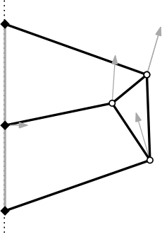
Consider the point-line graph shown in Figure 7(a). Two different realisations as a line-concurrent point-line framework are shown in (d) and (e). The framework in (d) has two lines with the same normal. We can use Theorem 4.4 to show that it is not infinitesimally fixed intercept rigid by taking to be the edge-set of sugraph of shown in (b). Then is as shown in (c) and the right hand side of the inequality of Theorem 4.4 is , which is greater than . On the other hand the realisaton shown in (e) is infinitesimally fixed intercept rigid. In particular if we evaluate the right hand side of the inequality of Theorem 4.3 for , we obtain so the inequality holds.
(a)
(b)
(c)
(d)
(e)
(f)
(g)
We will see in the next section that the generic version of Theorem 4.3 can be deduced from Theorem 2.5. However there seems to be no such reduction in the nongeneric case so we provide a direct proof. We first give several tools from matroid theory in Section 4.3.1 and delay the proof of Theorem 4.4 to Section 4.3.2. Finally in Section 4.3.3 we show that, if each line has a distinct normal, the combinatorial condition of Theorem 4.4 is equivalent to that of Theorem 4.3. Although the combinatorial condition in Theorem 4.3 is much simpler than that in Theorem 4.4, currently we have no direct proof of Theorem 4.3.
Before proceeding to the proof, we describe a consequence of Theorem 4.4 for bar-joint frameworks. Consider, again, the transformation given in Section 2, which converts a point-line framework to a bar-joint framework . Note that a line-concurrent point-line framework will be mapped to a bar-joint framework such that all the points in lie on a line, say a horizontal line. If the rotation on the sphere is done such that the north pole is mapped to a point on the equator (so that the north pole is finally mapped to a point at infinity after the projection to the plane), then in the isomorphism between the spaces of infinitesimal motions of and , we have that if and only if is in the horizontal direction. In other words each point for can only slide along the horizontal line. Therefore, the question about the fixed-intercept rigidity of can be rephrased as the rigidity question of bar-joint frameworks with horizontal slider joints on the ground. This transformation is illustrated in Figure 7(d),(e),(f),(g) and Figure 8(a),(b).
More formally, a bar-joint framework with horizontal slider joints is a tuple of a graph , , and , where will represent a set of slider joints. An infinitesimal motion of is an infinitesimal motion of with for all , and is said to be infinitesimally rigid if horizontal translations are the only possible infinitesimal motions of . By the rigidity transformation explained above, Theorem 4.4 can be restated as follows.
Theorem 4.5.
Let be a point-line graph with and let for each . Then can be realised as a minimally infinitesimally rigid bar-joint framework in with as a set of horizontal slider joints such that the coordinate of is if and only if
- •
,
- •
for each , and
- •
for all nonempty .
Note that Theorem 4.5 has no restriction on the coordinates of the slider joints. This is a much stronger statement than previous results [25, 12], where a certain genericity is assumed for the coordinates of slider joints. Such bar-joint frameworks with horizontal sliders frequently appear in the structural engineering literature, where sliders are often located on the horizontal ground.

(a)

(b)
)
4.3.1 Matroid preliminaries
Let be a graph which may contain loops and let be a positive integer. We assign a copy of to each vertex and let be the direct sum of those spaces over all vertices. For , let be the restriction of to the space assigned to . Consider the incidence matrix of an oriented , that is, the -matrix in which the entries in row with are in column , in column and elsewhere, and the entries in a row corresponding to a loop at are in column and elsewhere. This matrix gives a linear representation of a variant of the cycle matroid of . This matroid has rank equal to
where if has no loop and otherwise. We can obtain a linear representation of this matroid by assigning a one-dimensional vector space to each , where
with each edge . Then .
Next we take the direct sum of copies of , which gives a -dimensional vector space for each edge :
Clearly
| (32) |
We now establish a variant of equation (32). Suppose that a -dimensional vector is assigned to each loop . We then assign a vector space to by putting
where denotes the span of . Let be the set of loops in a graph .
Lemma 4.6.
| (33) |
Proof.
This is implicit in [12], but we give a direct proof since the claim is easy. A vector is in the orthogonal complement of if and only if for every and every . Such vectors form a -dimensional space. Among those vectors, a vector is in the orthogonal complement of if and only if is in the orthogonal complement of for every and every . Thus the orthogonal complement of has dimension equal to .
Another type of subspace which we will associate to each edge is
These subspaces give a linear representation of the bicircular matroid of , and we have
| (34) |
We will also need the following result of Lovász [14] which gives a geometric interpretation of the so-called Dilworth truncation of a matroid. We say that a hyperplane intersects a family of linear subspaces transversally if for every .
Lemma 4.7.
Let be a finite set and be a family of linear subspaces of . Then there exists a hyperplane which intersects transversally and is such that
| (35) |
where the minimum is taken over all partitions of .
4.3.2 Proof of Theorem 4.4
Proof of Theorem 4.4.
Let for each and let be the rigidity matrix of a framework representing the system (28)–(31). This is a -matrix whose rows are of one of the following four types:
where denote vertices in while denote vertices in (and unspecified entries are equal to zero). Since the set of the row vectors of indexed by the vertices in is linearly independent, is row-independent if and only if the projections of the remaining row vectors of onto the orthogonal complement of the space spanned by the row vectors indexed by form a linearly independent set. In other words, is row-independent if and only if the following -matrix is row-independent:
Note that, if for with , then the corresponding row in the above matrix becomes zero, and hence is necessary for to be minimally infinitesimally rigid. Thus in the following discussion we assume for all .
By taking a suitable linear combination of the two columns indexed by each to convert one of these columns to a zero column and then deleting this zero column, and using the fact that for all pairs , we may deduce that is row-independent if and only if the following -matrix is row-independent:
| (36) |
We will show that there is an injective map such that is row-independent if and only if
for all nonempty , implying the theorem.
To this end, we define the following linear subspace in for each :
Note that the linear subspaces are in the form of given in Section 4.3.1 with the underlying graph . Moreover, for , there is a correspondence between a loop in and an edge with . Therefore Lemma 4.6 gives
| (37) |
For each , we also define the following linear subspace in :
Note that the linear subspaces are in the form of given in Section 4.3.1 with the underlying graph obtained from by removing and regarding each edge in with as a loop at . Hence by (34)
| (38) |
Now we consider the direct sum of and , and let be the direct sum of and for each edge . Combining (37) and (38),
| (39) |
By Lemma 4.7, there is a hyperplane in intersecting transversally and satisfying (35). Denote a normal vector of by . Since the hyperplane intersects transversally, we may assume for with and for (since a small perturbation of will not change the property (35).)
We define by and show that is equal to the rank of given in (36). We will use the following claim, which directly follows from the definition of and the fact that if and only if and .
Claim 1.
A vector lies in if and only if:
- •
for , and is proportional to ;
- •
for wth , ;
- •
for , .
Since each is one-dimensional, Claim 1 implies that is equal to the row space of the -matrix having the following form:
By scaling each column indexed by a vertex in , this matrix is transformed to (as defined in (36)). In other words,
| (40) |
By (35), (39), and (40), we get where
and the minimum is taken over all partitions of into nonempty subsets. The function is submodular, nondecreasing and non-negative, since it determines the dimension of by (39). Hence induces the row matroid of by [4]. This implies that if and only if for all nonempty .
4.3.3 Proof of Theorem 4.3
Proof of Theorem 4.3.
By Theorem 4.4 it suffices to prove that the two combinatorial conditions in Theorem 4.3 and Theorem 4.4 are equivalent under the assumption that the normals are distinct.
For each edge set and each , recall that is a subset of . We let be the set of edges in incident to in . Then the counts of Theorem 4.3 and Theorem 4.4 can be written as
| (41) | ||||
| (42) |
respectively, where the count of Theorem 4.4 is simplified to (42) due to the assumption that the normals are distinct.
4.4 Mixed constraints
A natural question is how to generalise the results of Sections 4.1-4.3 to the case when the lines have a mixture of constraints. That is, some lines are completely fixed, some lines have fixed normals so can translate but not rotate, some lines can rotate about a fixed point but cannot translate, and some are unconstrained. We will extend the construction used in the proof of Theorem 3.1 to show that generic instances of this mixed constraint problem can be transformed to the unconstrained problem and then solved using Theorem 2.3.
Suppose we have a point-line graph which has various types of line vertices i.e. a set of fixed lines, a set of lines with fixed normals, a collection of pairwise disjoint sets of lines with a fixed centre of rotation, and unconstrained lines. A realisation of in is a framework together with a map , where is the centre of rotation for all lines in for each . We say that the constrained framework is generic if the set of coordinates are algebraically independent over .
We first consider the case when and . (In this case no rotation or translation of will satisfy the constraints on the lines of any generic realisation of .) We construct an unconstrained point-line graph by first adding a large rigid point-line graph to . We then choose a line-vertex in and add an edge from to each . This corresponds to the operation of adding the ‘tree of grey edges’ joining the (fixed-normal) line-vertices in Figure 6. For each set , we choose a distinct point-vertex in and add an edge from to each vertex of . This corresponds to the operation of adding a new point-vertex joined by ‘grey edges’ to each of the (fixed-intercept) line-vertices in Figure 8. Finally we join each to and a point-vertex of . This construction is illustrated in Figure 9.
Let and be generic realisations of and in so that for all , for all , and for all . Then has a non-zero infinitesimal motion if and only if has a non-zero infinitesimal motion which keeps fixed. Hence is infinitesimally rigid as a constrained point-line framework if and only if is infinitesimally rigid as an unconstrained point-line framework. Thus we may determine whether is infinitesimally rigid by applying Theorem 2.3 to . Note that our definition of the genericity of is independent of the choice of for . (This makes sense because the structure of the rigidity matrix given in Section 2.4 implies that the rank of will be maximised for any realisation such that the coordinates of are algebraically independent.) This means that we are free to choose the values of the such that, for each , each of the lines with passes through the the point , so we can take the lines in each to be concurrent as in Section 4.3 if we wish.
Similar, but simpler constructions, can be used when or .
5 Further remarks and open problems
The combinatorial condition in Theorem 2.5(c), Theorem 3.1(d),(e) and Theorem 4.1 can all be checked in polynomial time, see [11], [8, 11, 26] and [23], respectively. For the condition in Theorem 4.3, as shown in the proof, the right hand side of the count condition defines a submodular function , and hence one can decide whether the condition is satisfied in polynomial time by a general submodular function minimization algorithm. Currently we do not have a specialized efficient algorithm for this count.
We have obtained characterizations of fixed-line rigidity and fixed-intercept rigidity in Theorem 4.1 and Theorem 4.4 for a point-line framework with arbitrary normals for its lines. An interesting open problem is to derive an analogous result for fixed-normal rigidity. An important special case is the problem of characterizing fixed-normal rigidity for point-line frameworks in which the lines have been partitioned into parallel classes with generic normals (this was posed by Bill Jackson and John Owen at the rigidity workshop in Banff in 2015). In view of the relationship between fixed normal rigidity and scene analysis described in Section 3, this problem is challenging even when the underlying graph is naturally bipartite (as it is equivalent to understanding when an arbitrary -scene has only trivial realisations). We have constructed examples of (nongeneric) 2-dimensional naturally bipartite point-line frameworks with distinct line-normals which satisfy the count condition of Theorem 3.1 but are not fixed-normal rigid.
In [9, 22] the transfer of rigidity results between Euclidean spaces and spherical spaces was extended to Minkowski spaces and hyperbolic spaces (spheres in Minkowski space). Preliminary versions of these infinitesimal rigidity transfers appear in [21]. Applying these transfers, Theorem 2.5 transfers to frameworks with a designated coplanar subframework in Minkowski space and in hyperbolic space. However there are a number of further interesting questions in this direction such as extending our other results on point-hyperplane frameworks with various constraints on the hyperplanes. Since Minkowski space has the full space of translations for hyperplanes, it is a natural setting to extend the results of this paper.
In the setting of body-bar frameworks, including the specific setting of Body CAD frameworks, there are preliminary results [7, 12] which include (nongeneric) pinned and slider-joints, and point-line, as well as point-plane, distance constraints. These results and the results in this paper, can be refined and extended to explore body-bar-point frameworks - which do occur in built linkages in D and D. Some of these extensions and further related results will appear in the thesis [5].
Previous work on direction-length frameworks [24, 31] can be viewed as (i) combinatorially special fixed-normal point-line frameworks, with exactly two points joined to each line; and (ii) all point-line distances set as i.e. they are point-line incidences. With all this special geometry, the combinatorial characterization in [24] has one more condition than the characterization for general point-line frameworks in Theorem 4.2. This added condition comes from the fact that subgraphs with no point-point distance constraints can be dilated. An extension in which fixed normal lines are allowed to contain an arbitrary number of points is given in [17]. Many other extensions are open for exploration. These connections also suggest that prior results on parallel-drawings and mixed frameworks in higher dimensions, again with two vertices per line, such as [3, 32], can be generalized to combinatorially special fixed-normal point-hyperplane frameworks in higher dimensions.
Acknowledgements
We thank Banff International Research Station for hosting the 2015 workshop on ‘Advances in Combinatorial and Geometric Rigidity’ during which this work was started. We also thank HIM (Bonn) and ICMS (Edinburgh) for hosting further rigidity workshops in October 2015 and May 2016, respectively, and we thank DIMACS (Rutgers) for hosting the workshop on ‘Distance Geometry’ in July 2016. The discussions we had during these workshops played a crucial role in the writing of this paper.
References
- [1] R. Connelly and W. Whiteley, Global rigidity: the effect of coning, Discrete Comput. Geom., 43:4 (2010) 717–735.
- [2] H. Crapo and W Whiteley, Statics of frameworks and motions of panel structures, a projective geometric introduction, Topol. Struct. 6 (1982), 43–82.
- [3] H. Crapo and W Whiteley, 3-Space Reciprocals and Parallel Drawings, Preprint 1994, wiki.math.yorku.ca/index.php/Resources_in_Rigidity_Theory
- [4] J. Edmonds, Submodular functions, matroids, and certain polyhedra, in Combinatorial Structures and their Applications, eds. R. Guy, H. Hanani, N. Sauer, and J. Schönheim, Gordon and Breach, New York, 1970, 69-87.
- [5] Y. Eftekhari, Geometry of point-hyperplane and spherical frameworks, Ph.D. Thesis, York University, to appear, Spring 2017.
- [6] J. Graver, B. Servatius and H. Servatius, Combinatorial rigidity, Graduate Studies in Math., AMS, 1993.
- [7] K. Haller, A. Lee-St. John, M. Sitharam, I. Streinu, and N. White, Body-and-cad geometric constraint systems, Comput. Geom. 45(2012) 385-405.
- [8] H. Imai, On combinatorial structure of line drawings of polyhedra, Discrete Appl. Math. 10 (1985), 79-92.
- [9] I. Izmestiev: Projective background of the infinitesimal rigidity of frameworks, Geom. Dedicata, 140(2009) 183–203.
- [10] B. Jackson and T. Jordán, Rigid two-dimensional frameworks with three collinear points, Graphs and Combinatorics, 21:4 (2005) 427–444.
- [11] B. Jackson and J. Owen, A characterisation of the generic rigidity of 2-dimensional point-line frameworks, J. Comb. Theory: Series B, 119 (2016) 96–121.
- [12] N. Katoh and S. Tanigawa, Rooted-tree decompositions with matroid constraints and the infinitesimal rigidity of frameworks with boundaries, SIAM J. Discrete Math., 27:1, (2013), 155–185.
- [13] G. Laman, On graphs and rigidity of plane skeletal structures, J. Engrg. Math. 4 (1970), 331–340.
- [14] L. Lovász, Flats in matroids and geometric graphs, in Combinatorial Surverys (Proc. Sixth British Combinatorial Conf., Royal Hollaway College, 1977), Academic Press, London 1977 45–86.
- [15] D. Myska, Machines and mechanisms: applied kinematic analysis, Prentice Hall, 2012.
- [16] A. Nixon, J. Owen and S. Power, Rigidity of frameworks supported on surfaces, SIAM J. Discrete Math., 26:4 (2012) 1733–1757.
- [17] J. Owen and S. Power, Independence conditions for point-line frameworks, unpublished manuscript.
- [18] J. Owen, Algebraic solution for geometry from dimensional constraints, Proc. the first ACM Symposium on Foundations in Solid Modeling and CAD/CAM applications, (1991), 397–407.
- [19] A.V. Pogorelov, Extrinsic geometry of convex surfaces, Translation of the 1969 edition, Translations of Mathematical Monographs 35, AMS, 1973.
- [20] N. Rosenauer and A.H. Willis, Kinematics of Mechanisms, Dover Publications, New York 1967.
- [21] F. Saliola and W. Whiteley, Some notes on the equivalence of first-order rigidity in various geometries, Preprint (2007) arXiv:0709.3354.
- [22] B. Schulze and W. Whiteley, Coning, symmetry and spherical frameworks, Discrete Comput. Geom., 48 (2012) 622–657.
- [23] B. Servatius, O. Shai, and W. Whiteley, Combinatorial characterization of the Assur graphs from engineering, European Journal of Combinatorics 31, 2010, 1091–1104.
- [24] B. Servatius, and W. Whiteley, Constraining plane configurations in computer-aided design: Combinatorics of Directions and Lengths, SIAM J. Discrete Math. Vol. 12, 1999, pp. 136–153.
- [25] I. Streinu and L. Theran, Slider-pinning Rigidity: a Maxwell-Laman-type Theorem, Discrete Comput. Geom., 44 (2007), 812–837.
- [26] K. Sugihara, An algebraic and combinatorial approach to the analysis of line drawings of polyhedra, Discrete Appl. Math. 9 (1984), 77-104.
- [27] W. Whiteley, Rigidity and polarity I: statics of sheet structures, Geom. Dedicata, 22 (1987) 329–362.
- [28] W. Whiteley, Rigidity and polarity II: weaving lines and tensegrity frameworks, Geom. Dedicata, 23 (1989) 75–79.
- [29] W. Whiteley, A matroid on hypergraphs, with applications to scene analysis and geometry, Discrete Comput. Geom., 4 (1989), 75–95.
- [30] W. Whiteley, Some matroids from discrete applied geometry, in Matroid Theory, J. Bonin, J. Oxley and B. Servatius (eds.), AMS Contemporary Mathematics, 1996, 171–311.
- [31] W. Whiteley, Geometry of Direction and Length Frameworks, Preprint 1996, wiki.math.yorku.ca/index.php/Resources_in_Rigidity_Theory
- [32] W. Whiteley, Parallel Drawings in 3-Space, Preprint 1996, wiki.math.yorku.ca/index.php/Resources_in_Rigidity_Theory
- [33] W. Whiteley, Representing geometric configurations: computational approaches, in Learning and geometry, eds. D. Kuecher and C. Smith, Birkhauser, 1996, 143–177.