1Department of Physics, Stanford University, Stanford, CA 94305, USA
2Department of Physics, Harvard University, Cambridge, MA 02138, USA
Random tensor networks provide useful models that incorporate various important features of holographic duality. A tensor network is usually defined for a fixed graph geometry specified by the connection of tensors. In this paper, we generalize the random tensor network approach to allow quantum superposition of different spatial geometries. We setup a framework in which all possible bulk spatial geometries, characterized by weighted adjacient matrices of all possible graphs, are mapped to the boundary Hilbert space and form an overcomplete basis of the boundary. We name such an overcomplete basis as holographic coherent states. A generic boundary state can be expanded in this basis, which describes the state as a superposition of different spatial geometries in the bulk. We discuss how to define distinct classical geometries and small fluctuations around them. We show that small fluctuations around classical geometries define “code subspaces” which are mapped to the boundary Hilbert space isometrically with quantum error correction properties. In addition, we also show that the overlap between different geometries is suppressed exponentially as a function of the geometrical difference between the two geometries. The geometrical difference is measured in an area law fashion, which is a manifestation of the holographic nature of the states considered.
1 Introduction
The holographic duality[1, 2, 3] was proposed as a duality between quantum gravity in dimensions and quantum field theory in dimensions. The correspondence was originally proposed between the partition function and correlation functions of the two theories. The large limit of the boundary quantum field theory corresponds to the bulk semiclassical limit (the limit of small Newton constant ). The role of quantum entanglement in holographic duality was explicitly reflected by the Ryu-Takayanagi formula[4] and its generalizations[5, 6, 7, 8], which relates entanglement entropy of a boundary region to area of extremal surfaces. The relation of entropy and area motivated the proposal that tensor networks may provide a “microscopic” framework for understanding holographic duality[9, 10]. Tensor networks, or projected entangled pair states (PEPS) is an approach to construct entangled quantum many-body states[11, 12, 13, 14, 15, 16]. For a graph (see Fig. 1), the corresponding PEPS is obtained by first preparing an EPR pair for each link, and then projecting all qubits at the same vertex to a pure state specified by the tensor at that vertex. This procedure leads to a many-body state of the remaining qubits living at the end of dangling legs of the network. The advantage of the tensor network description is that the entanglement structure of the state is encoded explicitly in the geometry of the network. In particular, the entanglement entropy of each region is bounded by the minimal number of links that separate and its complement, multiplied by with the bond dimension of each tensor. This is the analog of RT formula.

To use tensor networks to understand holographic duality, a key question is what states correspond to semiclassical bulk geometry. As we learn in holographic duality, such states must satisfy various conditions[17, 18], such as the negative tripartite mutual information[19]. Various tensor network models[20, 21, 22, 23] have been proposed to incorporate desired features of holographic duality. Among them, the random tensor networks[23] are shown to realize many features of holographic duality naturally, including the RT formula with quantum corrections, and the quantum error correction property of the bulk-boundary holographic mapping[24]. However, there are holographic properties that are not reproduced by tensor networks, such as the Renyi entropy behavior[25, 8]. There are also obviously many other open questions that have not been addressed in the tensor network framework.
Among the open questions, an essential one is how to describe quantum superposition of different geometries, as is required for a quantum gravity theory. This is also a necessary step towards understanding Einstein equation and graviton excitations in the bulk. In this paper we make a small progress along this direction by setting up a framework for describing quantum superposition of tensor network states on arbitrary geometries. We generalize the random tensor network approach in Ref. [23] and define a linear map between geometries in the bulk and quantum states on the boundary. A geometry is described by the adjacient matrix of a weighted (unoriented) graph (with fixed number of vertices and arbitrary connectivity), which is defined as a basis vector in the bulk. The linear map defined by random tensors then maps each such basis state to a quantum state on the boundary, which is the holographic state that is dual to this geometry. With this linear map it is straightforward to take superpositions between different geometries. We prove that for a fixed size of the boundary, a large enough number of bulk vertices make such a mapping an isometry from the boundary to the bulk. In other words, parameterized by the weighted adjacient matrix form an overcomplete basis of the boundary, such that each state in the boundary Hilbert space can be mapped to a quantum superposition of different geometries. Due to the analog of boson coherent states (as will be elaborated more in later part of this paper), we name this basis of states “holographic coherent states”.
Furthermore, this formalism allow us to consider small fluctuation around a classical geometry, and show that such small fluctuations for a “code subspace”[24] which is mapped to the boundary isometrically. (The precise meaning of “classical geometry” and “small fluctuation” will be given later. In short, a classical geometry means all nonzero entries of the weighted adjacient matrix are large, while small fluctuations correspond to with .) Such small fluctuations can be considered as low energy states of the bulk quantum fields. The existence of bulk-boundary isometry in such subspaces guarantees that small fluctuations at different links of the graph are independent physical degrees of freedom. In other words, bulk locality emerges in such subspaces even if the whole bulk theory is intrinsically nonlocal. In addition, the bulk-boundary isometry satisfies the local reconstruction properties known in holographic duality. The structure of a boundary-to-bulk isometry in the whole boundary Hilbert space and a bulk-to-boundary isometry in code subspaces has been proposed as “bidirectional holographic code” in Ref. [22], which is schematically summarized in Fig. 2.
As an overcomplete basis, states for different geometry do not correspond to orthogonal states of the boundary. However, we show that the overlap between different geometries are exponentially suppressed in the large limit. This is similar to ordinary boson coherent states that are used in mean-field approximation of superfluids and superconductors. Different coherent states are not orthogonal. But because their overlap is exponentially small, it is physically meaningful to consider them as physically different states, and therefore consider the condensate wavefunction as a physical order parameter field. An interesting difference of the geometrical states from ordinary coherent states is that the overlap between two states has a “holographic” behavior. If two geometries and are distinct in a region and identical outside , we prove that the overlap is upper bounded by with the area of a minimal surface bounding region . is a constant determined by the entanglement entropy contributed by each link crossing the boundary. The area law form of the overlap is a manifestation of the fact that the states are consistent with the holographic principle—the fact that the physical degrees of freedom in a region are bounded by their area rather than volume.

The remainder of the article is organized as follows. In Sec. 2 we present the general setup of our approach. In Sec. 3 we study the condition of boundary-to-bulk isometry. In Sec. 4 we investigate the definition of classical geometries and the code subspaces with bulk-to-boundary isometry. In Sec. 5 we study the overlap between different classical geometries to show that distinct geometries are almost orthogonal. Finally, the conclusion and further discussions are given in Sec. 6.
2 General framework
We begin with a brief overview of the random tensor networks proposed in Ref. [23]. For a graph, such as the one in Fig. 1, one first prepares a EPR pair of two qudits for each link, denoted by . Then the RTN is defined by projecting all qudits on the site to a random pure state . If each qudit has dimension , and site has neighbors, is a random unit vector in a -dimensional Hilbert space. The probability distribution of is uniform, which means and has the same probability for any unitary . Alternatively, one can define with a Haar random unitary operator and a fixed reference state. For a graph , the RTN state is expressed as
| (1) |
with the runs over (unoriented) edges in the graph .
From the definition of RTN, it is natural to see how to generalize this formalism to include superposition of different geometries (graphs)—The link state can be replaced by superpositions of such states on different graphs. To make this well-defined, one needs to modify the definition slightly to make sure the Hilbert space dimension of each vertex is identical for different graphs. This can be easily achieved by defining some auxiliary states on links that are absent in . For each , define a state which is a direct product state and is orthogonal to . Adding such direct product states do not change the entanglement structure of the system. Then if we replace by , the dimension of each site is if the total number of vertices is . Therefore the random states can be chosen in a Hilbert space of dimension independent from . Denote as the “parent state” before projection, then the superposition of two geometries correspond to a boundary state . In other words, now we have a linear map between different graphs corresponding to different EPR pair configurations (in the same Hilbert space) to different boundary states.

Motivated by the discussion above, we consider a more general situation and define the following tensor network. Consider a complete graph with vertices, in which of them are labeled as “boundary” vertices, and the rest of them are bulk vertices. For each pair of vertices (), we define a three-leg tensor shown in Fig. 3, with and .11 1 Similar link variables have been introduced in perfect tensor networks in Ref. [26] for a different but related purpose. This tensor defines an isometry from index to indices . In other words, states
| (2) |
are orthonormal, i.e. . (Obviously this requires .) The link variables can be considered as specifying a weighted graph. Since we want the weight to label entanglement in state , we can require the entanglement entropy between and to be an increasing function of . For example, to be specific we can require
| (3) |
which means is the number of EPR pairs across the link, each with dimension . The maximal corresponds to a maximally entangled state.
In addition, each boundary vertex is connected with a EPR pair state which entangles a qudit at vertex with one at the boundary physical site . Then for each configuration , an RTN is defined by
| (4) |
If we only want to incorporate superposition of RTN on different graphs, the simplest choice will be , in which case a qubit at each link determines whether the link is connected (entangled) or not. However, it is more convenient to introduce a larger , which makes it possible to define “small” fluctuations around a classical geometry, as will be discussed in Sec. 4.
The definition (4) can be considered as a linear map between the boundary Hilbert space (with dimension ) and the bulk Hilbert space spanned by the link qudits (with dimension ). One can view this map as a holographic mapping that builds a correspondence between states (on the boundary) and geometries (in the bulk). It is straightforward to generalize the random average technique in Ref. [23] to the current setup, which is how we will investigate properties of this holographic mapping in the following sections.
3 Boundary-to-bulk isometry
In this section, we will study the holographic mapping from boundary to bulk, and show that it is an isometry under certain conditions. This result demonstrates that tensor network states for all configurations forms an overcomplete basis of the boundary Hilbert space, so that any boundary state can be expanded in this basis.
The isometry condition requires
| (5) |
If we view the tensor network in Fig. 3 as an entangled state between boundary and bulk link qudits, the isometry condition is equivalent to the statement that the reduced density matrix is maximally mixed. To study we study its second Renyi entropy
| (6) |
Similar to Ref. [23], we study the random average of the numerator and denominator separately, and then study their fluctuations. When the fluctuation is small, we have .
3.1 The random-averaged isometry condition
A commonly used trick in writing the Renyi entropy is to write
| (7) |
with the density matrix of the whole system, and the swap operator acting on two-copies of the system which permutes the two copies in region. More explicitly, if we denote an orthonormal basis of region as , then .
For the state defined in Eq. (4), is
| (8) | |||||
| (9) |
Therefore
| (10) | |||||
Here we have used the mathematical fact that the random average , with the swap operator defined in the same way as , acting on all qudits at site . The normalization constant .
The right-hand side of Eq. (10) is a sum over the purity of the state for different regions , with running over all subsets of the vertices. Since this state is simple, with only bipartite entanglement between different sites, the purity can be explicitly computed. In the same way as in Ref. [23], the sum can be expressed as a partition function of a classical Ising model, with an Ising spin defined on each site. Each spin configuration corresponds to a region which is defined as the spin domain. The action of the Ising model is defined such that . Since the state on the righthand side only contains bipartite entanglement, the Ising model action only contains one-body and two-body terms:
| (11) | |||||
Here is the second Renyi entropy of site in the state , i.e. , and the Ising coupling is half of the second Renyi mutual information between sites in the mixed state . The last term in the action sums over the boundary sites.
The Ising model problem is simpler than that for a generic RTN in Ref. [23] because all pairs of are coupled equally. Consequently, all bulk vertices are equivalent, and all boundary vertices are equivalent. The action is therefore only a function of two integers, the number of down spins in the bulk vertices , and the number of down spins in the boundary vertices .
| (12) |
The three terms are contributions of links within region , links between and its complement, and links from to the boundary, respectively, as is illustrated in Fig. 4.

With the action , Eq. (10) becomes
For large , this sum is dominated by the biggest term, which corresponds to the minimum of . One can show that reaches its minimum in the large limit at one of the corners in region . A detailed explanation can be found in Appendix.A.1. The same analysis applies to the denominator , and the only difference is in the boundary term .
with and .
The isometry condition is satisfied if the dominant configuration for both the numerator and the denominator is given by , which requires
| (23) | |||||
| (24) |
Condition (23) is simply a requirement that the bulk Hilbert space dimension is larger than that of the boundary (). Condition (24) requires that the link state is sufficiently entangled. In term of coupling , the condition (24) requires
| (25) |
3.2 Fluctuations
As we discussed earlier, the calculation of only tells us the average of second Renyi entropy if the fluctuation is small. The fluctuation can be studied by computing . As has been shown in Ref. [23], the random average of a quantity like , which is quartic in , can be expressed as a partition function of a statistical model with a pseudo-spin at each site taking values in the 4-element permutation group . In general, any quantity in the form of , with operator acting on copies of the system,22 2 For example, which determines the -th Renyi entropy can be written as with the cyclic permutation of the copies of systems in region. is mapped to a partition function of a model with pseudo-spins in -element permutation group . Similar to the Ising model analyzed above, the statistical models for higher is also defined on a complete graph, which simplifies the problem. In Appendix A we analyze these pseudospin models and obtain sufficient conditions for fluctuations such as to be controlled. For bounding the fluctuation of the second Renyi entropy calculation, the sufficient conditions are the following:
| (26) | |||||
| (27) |
with in the second equation. More details of the derivation will be given in Appendix A. It is not difficult to see that conditions (26) and (27) imply the conditions we obtain earlier in Eq. (23) (25). Condition (26) can be easily satisfied in large volume . Condition (27) imposes addition constraints to the choice of states and , but is also not hard to satisfy, as we will discuss in more details in Appendix A. We also give an explicit example of in Appendix A.3 which satisfies condition (27) for general .
4 Bulk-to-boundary isometry in code subspaces
Since the bulk basis is generically overcomplete, the mapping from bulk to boundary defined by our random tensor network is not injective. However, holographic duality requires that small fluctuations around a classical geometry are independent physical states on the boundary. For example, if we consider a dilute gas of gravitons in the bulk, the total degree of freedom of the gas is proportional to volume. Gravitons at different bulk locations should be dual to independent degrees of freedom on the boundary, since graviton creation/annhilation operators should be mapped to independent operators on the boundary by the dictionary of holographic duality. This requirement means that there should be a bulk-to-boundary isometry in the subspace of such small fluctuations. The bulk small fluctuations are mapped to a subspace of the boundary Hilbert space, named as the “code subspace”[24, 21]. Each geometry corresponding to a configuration defines a code subspace . The mapping of such small fluctuations to the boundary should satisfy the following local reconstruction property: Each region on the boundary corresponds to a minimal surface in the bulk that is homologous to it. The region enclosed by is the entanglement wedge 33 3 More precisely, here is the intersection of the entanglement wedge and the spatial slice. Since we will always be dealing with a spatial slice, we neglect this difference and call the entanglement wedge.. A bulk operator acting in the subspace of small fluctuations (the code subspace) in the bulk region can be reconstructed in boundary region . Since each bulk point can be enclosed by the entanglement wedges of different boundary regions, information in the bulk can be recovered from different boundary regions, making the bulk-boundary map in the code subspace a quantum error correction code[24]. The bulk-boundary isometry and local reconstruction is illustrated in Fig. 5.

In the following we will explain how our formalism of fluctuating geometry allows the definition of small fluctuations and code subspaces. We first define classical geometries and small fluctuations in our setup, and then study the ovelaps between different classical geometries to verify that macroscopically different geometries indeed correspond to almost orthogonal states on the boundary.
4.1 Classical geometry and the code subspace
Each configuration corresponds to a “geometry” (i.e. a weighted graph), but if takes arbitrary values, one cannot define what fluctuations are considered “small”. With a large link variable dimension , one can define a classical geometry as one with all nontrivial links () contributing a large entropy , and then define small fluctuations as fluctuations of that are small compared to .
For concreteness, we pick a value of link variable with , and take the limit with fixed. We define a classical geometry by a state with all equal to either or . 44 4 It is straightforward to generalize the following discussion to states with different on different links as long as all of them are taken to infinity with the ratio fixed. For such states, we can define an adjacient matrix with , such that .
Now define a range of small fluctuation . In the limit , is kept finite. Then we define small fluctuations around the classical geometry as all states satisfying
This range of defines a subspace of the bulk, which is mapped to the boundary by the random tensor network. The definition of the classical geometry and small fluctuation subspace is illustrated in Fig. 6.

To study whether the bulk-boundary map is an isometry, we carry the same calculation as in Sec. 3 to evaluate the second Renyi entanglement entropy between bulk and boundary. An isometry is defined if the bulk subspace is maximally entangled with the boundary. The calculation is exactly parallel to that in Sec. 3, except that the bulk link state in Eq. (8) is replaced by
The Ising action is changed correspondingly to
| (34) | |||||
Here are half the Renyi mutual information of strong and weak link states in Eq. (4.1), respectively. In the limit of , with and finite, is the leading term in the action, and is a subleading correction.
The analysis of this action is essentially the same as the original RTN case in Ref. [23]. The boundary term prefers , while the bulk pinning field prefers . Isometry condition is satisfied in the limit if the lowest action configuration is everywhere, which corresponds to an entropy . In order for this configuration to have the lowest action, one requires that creating any spin up domain costs a positive action. Denoting the action of a spin configuration with in and elsewhere as , the isometry requirement is
| (35) | |||||
where the first two terms are action cost from the two-body interaction terms, the third term is the action cost from boundary pinning fields, while the last term is the action saved by the external field term . is the number of vertices in and is the number of links connecting and its complement in graph (excluding the boundary links). is the number of links connecting with boundary, i.e. the number of boundary sites in .
For sufficiently large and finite , condition (35) is satisfied. To obtain a more explicit understanding on the requirements, in the following we derive a sufficient condition which guarantees that the isometry condition (35) is satisfied for all classical geometries. Denote and as the number of interior sites and boundary sites in , respectively, such that and . The action cost is a function of and the graph dependent parameter . If we are considering a particular given graph, is not independent from and . However, simplification occurs when we require condition (35) to hold for all and for all classical geometries. By varying the graph, one can always vary of a given region in the range ). Therefore we can view the action cost as a function of three independent variables . This simplified the problem of minimizing , because the function in Eq. (35) does not have local minimum in term of and . Thus the minimum can only occur at corners of the parameter space. Given that , the minimum always occurs at , in which case . Evaluating at the four corners or and or leads to two nontrivial conditions:
| (36) | |||||
| (37) |
In summary the two sufficient conditions are
| (38) | |||||
| (39) |
Physically, the first condition (38) is simply the requirement that the bulk code subspace has smaller dimension than the boundary. The second condition requires that even weak links with coupling provide strong enough entanglement to propagate information from bulk to boundary isometrically. It should be noted that condition (38) requires to grow exponentially with volume (if we fix the ratio ). This is necessary since the bulk code subspace dimension grows with . Besides, Eq.39 only requires to be a number in this limit. If we consider a limit with large but finite , it will be impossible to faithfully represent all link variable fluctuations to the boundary. However, it is probably still possible to define a code subspace with lower bound dimension, which contains bulk excitations with a low enough density. (An example of such kind of code subspace was discussed in Ref. [22].) Such a code subspace which is not a direct product of Hilbert spaces of each link is probably closer to the code subspace in AdS/CFT, consisting low energy bulk quantum field theory excitations.
4.2 Local reconstruction properties
Now we further investigate the local reconstruction properties of the bulk-boundary isometry. The local reconstruction requirement can be phrased in an entanglement entropy calculation. In the old setup of tensor networks with fixed geometry, shown in Fig. 5, one can view the bulk-boundary map as a quantum state that contains four partitions . The requirement that contains all information about is equivalent to the statement . In the following we will evaluate the second Renyi entropy version of the mutual information. In the large limit when the fluctuation of Renyi entropies are small, we expect the von Neumann entropy to be equal to the Renyi entropy. Before proceeding, we would like to note that in the current setup the bulk degrees of freedom are defined on links, so that the bulk Hilbert space do not factorize into different regions. For a boundary region , one can still define an entanglement wedge , such that all edges with both ends contained in can be reconstructed from . This is illustrated in Fig. 7.
Since we need to compute Renyi entropy of regions including both bulk and boundary, we should not trace over bulk link variables to obtain a reduced density matrix . Instead we treat the whole RTN with bulk and boundary indices as a state, and map the second Renyi entropy calculation to an Ising model partition function. All dangling ends of the tensor network in bulk and boundary correspond to fixed external spins that couple to the dynamical Ising spins defined on bulk vertices. We denote the dynamical Ising spins as , and the external spins as on the boundary and on bulk links. all take values of . When we compute the Renyi entropy of a bulk region and a boundary region , the external spins are defined as
For small fluctuations around a graph considered here, we have
| (45) | |||||
and are the same as in Eq. (34). The earlier calculation of the entropy of entire boundary in Eq. (34) corresponds to the special case and . The constant prefactor is not important as it is the same for all configurations, and does not affect normalized quantities such as . Similarly, and can be computed by the same action with different boundary conditions.
The mutual information is determined by the correlation between external spins mediated by the dynamical spins. We denote the effective action as the effective action with boundary condition (4.2), with labeling the sign of external spin in and respectively. Similarly , and is the normalization constant. Then
| (46) |
is determined by the “energy cost” of the external spins in and being anti-parallel. The requirement of zero mutual information is equivalent to the requirement that the two external spins are completely uncorrelated. It is easy to see that this is true in the limit we consider, with and finite. In this limit, the spin configuration is completely determined by boundary external spins , and thus . For finite , the local reconstruction condition depends on more detailed properties of the classical geometry. Although it is possible to write down some sufficient condition by taking and to be very large, we feel these conditions are not so useful to include here.
5 Overlap between different classical geometries
In the discussion above we have shown that each classical geometry labeled by a graph is accompanied with a code subspace that satisfies bulk-boundary isometry and local reconstruction properties. The next question is whether the code subspaces for different classical geometries are truely independent subspaces of the boundary Hilbert space. Since the basis is over-complete, different geometries are generically not orthogonal, but in the following we will show that states in the code subspace of different classical geometries have exponentially small overlap.
For this purpose we study the overlap between two generic geometries and . Using the definition (4) we have
| (47) |
Carrying the random average one obtains
| (48) |
It is essential to go to the second order and study the fluctuation around the average value, so that we evaluate :
with . To simplify this expression we can write with the swap of all bulk vertices. will simply permute and . Relabel by we obtain
| (50) | |||||
Here is the reduced density matrix of in region , and similarly for . If we consider the term with the entire bulk, is the inner-project of the two bulk states. Roughly speaking, we can consider all other terms as corrections to the overlap induced by the bulk-boundary map that is not injective.
The overlap is nonzero only if for all . Denote the set of that satisfy this property as . To obtain an upper bound of the overlap, we use the inequality
| (51) |
where are the second Renyi entropy of states and in region . Therefore
| (52) |
To understand the physical meaning of Eq. (52), we evaluate it in several situations.
- 1.
The diagonal element. If , can be any subset of the bulk, and the dominant term in the sum is given by . Also in this case, the inequality takes the equal sign. If we take the classical geometry discussed in this section, with , we can ignore the contribution of other terms, and obtain . Therefore
(53) The ratio is close to in the limit of large volume since and are much smaller than . In other words, the fluctuation of the norm of state is exponentially suppressed, which justifies the computation of without first normalizing the two states.
- 2.
Completely distinct states. If we consider two completely distinct states such that , then the only contribution comes from , and . In other words, the overlap between these states, after normalization, is the inverse of boundary Hilbert space dimension . This is equal to the average overlap between two completely random states in the boundary Hilbert space dimension. 55 5 Apparently, when the bulk volume is large enough so that the basis is very overcomplete, some of them will have a significant overlap. This fact, however, does not appear in the calculation of averaged overlap . The higher moments shall be able to reveal the effect of extremely large , which we postpone to future works. We would like to thank Lenny Susskind for helpful discussion on this problem.
- 3.
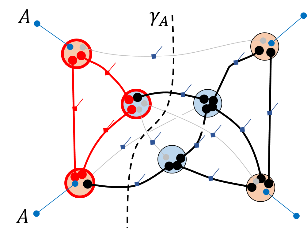
Two states different in IR. Now we study a nontrivial example. In holography all geometries considered are asymptotically anti-de Sitter space in UV (the region near the boundary) and are generically different in IR. For example we may consider two geometries, one with a black hole in IR and one without black hole. As a toy model of this situation, we can consider two geometries that are identical in a UV region bounding the boundary, and distinct in the IR region, as is illustrated in Fig. 8. We assume and are completely distinct if or are outside region , so that all regions contributing to the overlap are or its subsets. In this case the dominant contribution to Eq. (52) is given by the that has minimal averaged entropy . If both geometries are classical geometries with all connected links , the entropies satisfy area law with the entropy contributed by each link state . denotes the area (number of links crossing the boundary of ) in graphs of respectively. In summary we obtain for two classical geometries
(54) where is chosen to minimize the averaged area. For example if we consider two geometries with and without a black hole, and assume that the geometry to be identical in UV until a certain distance to the horizon, then is bounded by the area of black hole horizon, so that the overlap is upper bounded by . More generally, the overlap is bounded by the entropy of the minimal area surface that enclose the region where the two geometries are (macroscopically) distinct.

From our definition of code subspace, it’s clear that if two classical geometries are distinct at a link , the small fluctuations are still distinct from . Therefore the overlap upper bound for between two classical geometries also applies to any pair of states from the code subspaces of and . Consequently, if we choose a set of macroscopically distinct geometries , the code subspaces of each of them are almost orthogonal subspaces of the boundary Hilbert space. One can define a bigger code subspace such that the bulk-boundary isometry is still well-defined in the bigger code subspace. In the bigger code subspace , operators that can be reconstructed on a boundary region form an algebra with nontrivial center, a structure that has been investigated in Ref. [28]. We would like to comment a bit more on the mapping between bulk and boundary operators. A generic bulk operator in this code subspace has the form , with the projection operator onto -th code subspace , and an operator acting only in that subspace. If we denote the linera map from boundary to bulk as , a local operator in the code subspace of geometry is mapped to a boundary operator . Although the bulk-boundary mapping is linear and isometric, one can consider as the linear map restricted to a code subspace, which is “state-dependent”[29]. Locality in the bulk can only be defined in a code subspace around a given classical geometry, and the local operators in a code subspace (such as an operator that only slightly changes value for one link) is actually an operator in the large bulk Hilbert space. The “state dependence” of operator correspondence in each code subspace is encoded in the support of the operator in the bulk Hilbert space, specified by .
6 Conclusion and discussions
In conclusion, we have shown that the random tensor network states on all graphs form an overcomplete basis of the boundary Hilbert space, which we name as holographic coherent states. A generic boundary state is mapped to a superposition of geometries. The semiclassical geometries are defined as small fluctuations around reference classical geometries with strongly entangled edges. We show that small fluctuations around a classical geometry form a code subspace, the states in which are mapped to the boundary isometrically, with local reconstruction properties. Furthermore, we show that states in the code subspaces of two different classical geometries are almost orthgonal to each other, with their overlap decaying exponentially as a function of the minimal area surface that covers the bulk region in which the two bulk geometries are distinct.
The holographic coherent state basis has a lot of similarity to the coherent state basis of a boson field. If we consider a complex boson field described by a theory, the coherent state basis is an overcomplete basis of the system, with which one can write a path integral representation of the partition function. The action of the system may have multiple local minima, for example configurations with and without vortices. Around each local minimum one can expand the action in small fluctuations, . The quantization of such fluctuations are low energy quasiparticles such as superfluid phonons. The Hilbert space of such quasiparticle excitations is a “low energy subspace” of the entire Hilbert space. Different classical minima are not exactly orthogonal, but the overlap of macroscopically different states are exponentially suppressed. Therefore one can view the low energy excitations associated with each of them as physically independent subspaces. 66 6 It is interesting to note that the theory example appeared in a related discussion in Ref. [30] about state-dependent operators (see Sec. 5). There are two key differences between the holographic coherent states we consider and the boson coherent states. Firstly, the overlap in the former case is suppressed by exponential of the minimal area covering the distinct region, while that in the latter case is suppressed by exponential of the volume of the distinct region, which can be viewed as a manifestation of holographic principle. Secondly, in the gravity case, locality in the bulk is only defined in the code subspaces, which can be seen in the fact that the log of Hilbert space dimension is proportional to the volume of the bulk, while that of the total Hilbert space is proportional to the boundary. On comparison, in ordinary boson coherent state case both quantities are proportional to the volume of the system.
There are a lot of open questions along this direction. For a given boundary Hamiltonian, a natural problem is to use the holographic coherent states as variational wavefunctions. The geometry described by can be used as a “mean-field order parameter” that is optimized by minimizing the energy. The difficulty of this approach is the random average, which introduces the ambiguity of a local unitary transformation and therefore mixes states with very different energy. In principle, this problem can be solved in the following procedure. For each given geometrical state , one can consider all local unitary transformations , with , and variationally determine by minimizing energy. Denote the minimal energy in this class of states as , we can then minimize energy to determine the optimal bulk geometry . It is not clear whether such a variational procedure is technically feasible. We will reserve that to future works.
Another natural question is how to obtain the bulk equation of motion—the analog of Einstein’s equation. By writing the boundary dynamics into a path integral in the geometrical basis, one can in principle obtain a bulk action. Is the Einstein equation or its analog the saddle point equation if the bulk action? Will such saddle point equation be related to previous entanglement approaches to Einstein equation[31, 32, 33, 34, 35, 36]. Yet another interesting question is whether a similar area-law bound of state inner product exists in general relativity, where the inner product between two states is defined by a path integral with these states as boundary conditions[37, 38]. It is interesting to compare our results with other recent discussions about the overcompleteness of the geometry basis.[39, 40, 41]
Acknowledgement. We would like to acknowledge helpful discussions with Ahmed Almheiri, Patrick Hayden, Aitor Lewkowycz, Don Marolf, Sepehr Nezami, Leonard Susskind and Michael Walter. This work is supported by the National Science Foundation through the grant No. DMR-1151786 (ZY), and the David and Lucile Packard Foundation (XLQ).
Appendix A Fluctuations and higher Renyi entropies
In Sec.3, we make the following approximation in the calculation of the second Renyi entropy.
| (55) |
where , denote the boundary field configuration for the calculation of , . This calculation is valid if the fluctuation around the minimum is small [23]. Formally, the following conditions should be satisfied , which can be achieved by requiring
| (56) |
Here we have used that , since at finite temperature the partition function receives contributions from all spin configurations, not just the minimal energy configuration. Similarly for the calculation of one can require . Thus the calculation of the fluctuation requires the random average over four copies of the density matrix. Similarly, when calculating the th Renyi entropy, we need to calculate which involves copies of the density matrix. For example and are both average of copies of density matrices, with different boundary conditions which specify the contraction of indices. More explicitly they can be written as and with the cyclic permutation acting on -copies of , and the permutation of and acting on the same region.
Therefore in general we can evaluate the random average of copies of density matrix with an arbitrary boundary condition, and study how to control its deviation from the contribution of the dominant configuration. The copy quantity with most general boundary condition can be expressed as
| (57) | |||||
with boundary permutations defining the boundary conditions. We label the permutation group elements as , with the identity operator. The averaged entanglement quantity is mapped to a partition function of a statistical mechanical model defined on the complete graph.
In the following we will prove that the fluctuation of such quantities with general boundary conditions is bounded if the following sufficient conditions are satisfied:
| (58) | |||
| (59) |
In Sec.A.1, we bound the fluctuations based on conditions 58 and Eq.59. In Sec.A.2, we propose a stronger condition of the density matrix that implies Eq.59. In Sec.A.3, we construct the an explicit example in spin system and show that Eq.58 and Eq.59 are satisfied.
A.1 General results
In this section, we prove that Eq.58 and Eq.59 are sufficient to bound the fluctuations and to guarantee that higher Renyi entropies are close to the maximum.
Next, it is straightforward to show that Eq.59 implies , , a condition we will use to bound the fluctuation. If we take , Eq.59 means
| (62) |
Since is normalized. . Thus .
Now we calculate the partition function in () replica with an arbitrary boundary condition. Using permutation symmetry between vertices in the complete graph, Eq. 57 can be rewritten as
| (63) | |||||
| with | |||||
where is the number of bulk(boundary) points occupied by the group element ; is the total number of bulk(boundary) points; fixes the boundary condition.
Then we replace , . Since , we have
| (64) | |||||
In the large limit, we treat and as continuous variables to decide where reaches its maximum. We use Stirling formula and calculate the second derivatives of this function
| (65) | |||||
Now we show that does not have local minimum away from the corners of the parameter space. A local minimum requires to be a negative definite matrix, so to prove that does not have local minimum one just needs to show that is not negative definite anywhere away from the corners. A corner of the parameter space (labeled by ) is defined by having one and all other numbers vanishing. Therefore for any point away from these corners, there are either two numbers of order , or two numbers of order . Let’s assume there are of order since the discussion with is exactly in parallel. This includes the following two cases:
- •
If is of , then there are two , with of order . Define a vector whose th element is , th element is and all others are . Obviously,
(66) Since , and , are , . So is not negative definite and there is no local maximum in this case away from the corners.
- •
If is of , then there is at least another being . We choose whose only non-zero element is at the th element. Thus
(67) Since is and , is , .
Therefore we conclude that Eq.59 is the sufficient condition that guarantees does not have local minimum away from the corners.
The next step is to compare the value of of each corner solution and bound the near corner solutions. The corner solutions are categorized as
- •
: , ,
(68) - •
: , , ,
(69) - •
: , , ,
(70) - •
: , , ,
(71)
Firstly, we notice that is always true, because is assumed and , where denotes the number of cycles in a permutation .
Secondly,
| (72) | |||||
In the inequality, we use , and the triangle inequality of , which is equal to the minimal number of transpositions (i.e., permutations that exchange only two indices) required to write a permutation . defines a distance on , which satisfies the triangle inequality [23]. Thus Eq.58 is a sufficient condition for .
Thirdly,
| (73) | |||||
where in the first inequality, we use and . In the second inequality, we use the triangle inequality of again. Thus if Eq.58 holds, we also have .
In fact, we can make tighter bounds in and if we do not simply discard or . However, using condition Eq.58 has the advantage that it does not depend on and the details of the link state.
Finally, we can bound by analyzing the configurations near the corners. We have shown that when Eq.58 and Eq.59 are satisfied, all other corner solutions are exponentially small compared with the dominating corner , and the exponent is suppressed by . Thus the next biggest configuration is at the neighborhood of the corner solution . In fact we can bound all configurations that are finite distance away from by , where is a number. Thus we obtain that
| (74) |
where is the total number of configurations of .
A.2 A sufficient condition for Eq.59
In this section, we provide a sufficient condition that deduces Eq.59, which helps to clarify what density matrices satisfy this equation. In a basis of the -copied Hilbert space, density operators and permutation operators are written as
| (75) | |||||
| (76) |
One can rearrage the indices and write
| (77) | |||
| (78) | |||
| (79) |
where in the last step, we have used the fact that the matrix elements in the product basis are real. In this representation, becomes an inner product between states with metric . Therefore Eq.59 follows from Cauchy-Schwarz inequality if is Hermitian and positive semi-definite for all . Thus we conclude that a sufficient but not necessary condition for Eq.59 is that is Hermitian and positive semi-definite. This condition is not necessary since Eq. (59) is only required for permutation operators and does not need to hold for general operators.
A.3 An explicit example of states
In this section, we provide an explicit example of link states and prove that condition (Eq.27) is satisfied. We define the state as a SU(2) singlet formed by two spins each carrying spin representation:
| (80) |
with labeling the link states. The Hilbert space of each site is a direct sum of different representations . States with different obviously are orthogonal. (A subtlety is that the entropy of state is , so that we should think the link variable if we still want to label the entropy across the link. This does not affect any discussion here.) The density matrix is given by
| (81) |
If one directly obtains in Eq. (78) for , the resulting is Hermitian but not positive semi-definite. However, we can prove satisfies condition (59) by defining a unitary operator on the site
| (82) |
The density matrix in the new basis is
| (83) |
Since commutes with permutation operators , we have . For , the corresponding operator defined in Eq. (78) is
| (84) |
with an identity matrix of the size . Obviously is diagonal and positive definite, so that we prove and therefore satisfy Eq. (59).
References
- [1] Edward Witten. Anti-de sitter space and holography. Advances in Theoretical and Mathematical Physics, 2:253–291, 1998.
- [2] Steven S Gubser, Igor R Klebanov, and Alexander M Polyakov. Gauge theory correlators from non-critical string theory. Physics Letters B, 428(1):105–114, 1998.
- [3] Juan Maldacena. The large-n limit of superconformal field theories and supergravity. International journal of theoretical physics, 38(4):1113–1133, 1999.
- [4] Shinsei Ryu and Tadashi Takayanagi. Holographic derivation of entanglement entropy from the anti–de sitter space/conformal field theory correspondence. Physical review letters, 96(18):181602, 2006.
- [5] Veronika E Hubeny, Mukund Rangamani, and Tadashi Takayanagi. A covariant holographic entanglement entropy proposal. Journal of High Energy Physics, 2007(07):062, 2007.
- [6] Thomas Faulkner, Aitor Lewkowycz, and Juan Maldacena. Quantum corrections to holographic entanglement entropy. Journal of High Energy Physics, 2013(11):1–18, 2013.
- [7] Xi Dong, Aitor Lewkowycz, and Mukund Rangamani. Deriving covariant holographic entanglement. arXiv preprint arXiv:1607.07506, 2016.
- [8] Xi Dong. The gravity dual of rényi entropy. Nature Communications, 7, 2016.
- [9] Brian Swingle. Entanglement renormalization and holography. Physical Review D, 86(6):065007, 2012.
- [10] Brian Swingle. Constructing holographic spacetimes using entanglement renormalization. arXiv preprint arXiv:1209.3304, 2012.
- [11] Steven R White. Density matrix formulation for quantum renormalization groups. Physical Review Letters, 69(19):2863, 1992.
- [12] Steven R White. Density-matrix algorithms for quantum renormalization groups. Physical Review B, 48(14):10345, 1993.
- [13] Frank Verstraete, Diego Porras, and J Ignacio Cirac. Density matrix renormalization group and periodic boundary conditions: a quantum information perspective. Physical review letters, 93(22):227205, 2004.
- [14] Frank Verstraete and J Ignacio Cirac. Renormalization algorithms for quantum-many body systems in two and higher dimensions. arXiv preprint cond-mat/0407066, 2004.
- [15] Guifré Vidal. Class of quantum many-body states that can be efficiently simulated. Physical review letters, 101(11):110501, 2008.
- [16] Zheng-Cheng Gu and Xiao-Gang Wen. Tensor-entanglement-filtering renormalization approach and symmetry-protected topological order. Physical Review B, 80(15):155131, 2009.
- [17] Idse Heemskerk, Joao Penedones, Joseph Polchinski, and James Sully. Holography from conformal field theory. Journal of High Energy Physics, 2009(10):079, 2009.
- [18] Sheer El-Showk and Kyriakos Papadodimas. Emergent spacetime and holographic cfts. Journal of High Energy Physics, 2012(10):1–72, 2012.
- [19] Patrick Hayden, Matthew Headrick, and Alexander Maloney. Holographic mutual information is monogamous. Physical Review D, 87(4):046003, 2013.
- [20] Xiao-Liang Qi. Exact holographic mapping and emergent space-time geometry. arXiv preprint arXiv:1309.6282, 2013.
- [21] Fernando Pastawski, Beni Yoshida, Daniel Harlow, and John Preskill. Holographic quantum error-correcting codes: Toy models for the bulk/boundary correspondence. arXiv preprint arXiv:1503.06237, 2015.
- [22] Zhao Yang, Patrick Hayden, and Xiao-Liang Qi. Bidirectional holographic codes and sub-ads locality. Journal of High Energy Physics, 2016(1):1–24, 2016.
- [23] Patrick Hayden, Sepehr Nezami, Xiao-Liang Qi, Nathaniel Thomas, Michael Walter, and Zhao Yang. Holographic duality from random tensor networks. arXiv preprint arXiv:1601.01694, 2016.
- [24] Ahmed Almheiri, Xi Dong, and Daniel Harlow. Bulk locality and quantum error correction in ads/cft. Journal of High Energy Physics, 4(2015):1–34, 2015.
- [25] Xi Dong. Shape dependence of holographic rényi entropy in conformal field theories. Physical review letters, 116(25):251602, 2016.
- [26] William Donnelly, Ben Michel, Donald Marolf, and Jason Wien. Living on the edge: A toy model for holographic reconstruction of algebras with centers. arXiv preprint arXiv:1611.05841, 2016.
- [27] Bryce S DeWitt. Quantum theory of gravity. i. the canonical theory. Physical Review, 160(5):1113, 1967.
- [28] Daniel Harlow. The ryu-takayanagi formula from quantum error correction. arXiv preprint arXiv:1607.03901, 2016.
- [29] Kyriakos Papadodimas and Suvrat Raju. An infalling observer in ads/cft. Journal of High Energy Physics, 10, 2013.
- [30] Daniel Harlow. Aspects of the papadodimas-raju proposal for the black hole interior. arXiv preprint arXiv:1405.1995, 2014.
- [31] Nima Lashkari, Michael B Mcdermott, and Mark Van Raamsdonk. Gravitational dynamics from entanglement” thermodynamics”. Journal of High Energy Physics, 2014(4):1, 2014.
- [32] Thomas Faulkner, Monica Guica, Thomas Hartman, Robert C Myers, and Mark Van Raamsdonk. Gravitation from entanglement in holographic cfts. Journal of High Energy Physics, 2014(3):1, 2014.
- [33] Brian Swingle and Mark Van Raamsdonk. Universality of gravity from entanglement. arXiv preprint arXiv:1405.2933, 2014.
- [34] Ted Jacobson. Entanglement equilibrium and the einstein equation. Physical review letters, 116(20):201101, 2016.
- [35] Seth Lloyd. The quantum geometric limit. arXiv preprint arXiv:1206.6559, 2012.
- [36] Erik Verlinde. On the origin of gravity and the laws of newton. Journal of High Energy Physics, 2011(4):1–27, 2011.
- [37] James B Hartle and Stephen W Hawking. Wave function of the universe. Physical Review D, 28(12):2960, 1983.
- [38] Juan Maldacena. Eternal black holes in anti-de sitter. Journal of High Energy Physics, 2003(04):021, 2003.
- [39] Daniel Louis Jafferis. Bulk reconstruction and the hartle-hawking wavefunction. arXiv preprint arXiv:1703.01519, 2017.
- [40] Yasunori Nomura, Nico Salzetta, Fabio Sanches, and Sean J Weinberg. Toward a holographic theory for general spacetimes. arXiv preprint arXiv:1611.02702, 2016.
- [41] Yasunori Nomura, Nico Salzetta, Fabio Sanches, and Sean J Weinberg. Spacetime equals entanglement. arXiv preprint arXiv:1607.02508, 2016.