Precise determination of the three-quark potential in SU(3) lattice gauge theory

We perform simulations of SU(3) lattice gauge theory (lattice QCD within the quenched approximation) in four dimensions with the lattice volume $L^{3}\times T$ and the lattice spacing $a$ by imposing periodic boundary conditions in all space-time directions. The three-quark potential is extracted from the PLCF as follows.

We first define a three-link correlator as

which is a direct product of three time-like link variables $U_{4}(x)$ placed at a time $x_{0}$ with spatial positions of three quarks, $\vec{x}_{1}$, $\vec{x}_{2}$, and $\vec{x}_{3}$. Greek indices $\alpha$, $\beta$, $\gamma$, $\delta$, $\epsilon$, $\zeta$ take the values from one to three, respectively. Practically, a three-link correlator is a complex matrix with $3^{6}=729$ components. The three-link correlator acts on a color state in the ${\bf 3}\otimes{\bf 3}\otimes{\bf 3}$ representation of the SU(3) group $|n_{\alpha\beta\gamma};\vec{x}_{1},\vec{x}_{2},\vec{x}_{3}\rangle$, which is an eigenstate of the hamiltonian $\mathbb{H}$ defined by the transfer matrix in the temporal gauge, $\mathbb{T}\equiv e^{-\mathbb{H}a}$, and then satisfies

where $n$ is the principal quantum number and repeated Greek indices $\alpha$, $\beta$, $\gamma$ are to be summed over from one to three. The energies $E_{n}(\vec{x}_{1},\vec{x}_{2},\vec{x}_{3})$ are positive and are common to all of the $3^{3}=27$ color components of $|n_{\alpha\beta\gamma};\vec{x}_{1},\vec{x}_{2},\vec{x}_{3}\rangle$. The multiplication rule of two three-link correlators for adjacent times at $x_{0}$ and $x_{0}+a$ is

With this multiplication rule a new and longer three-link correlator is created as schematically shown in Fig. 2.

We then construct the PLCF from the time-ordered product of the three-link correlators,

By inserting the complete set of eigenstates,

at each time $x_{0}=0,a,...,T-a$, and by using the normalization condition,

the expectation value of the PLCF is reduced to

The ground state potential, $V_{3q}\equiv E_{0}$, is then extracted as

where the terms of $O(e^{-(E_{1}-E_{0})T}/T)$ are always negligible at zero temperature. Therefore, once the PLCF is computed accurately for a large temporal extent $T$, it is straightforward to extract the ground state potential. For instance, if we refer to the value $a(E_{1}-E_{0})\sim 0.5$ at $\beta=6.00$ given by Takahashi and Suganuma [29], the order of magnitude of $O(e^{-(E_{1}-E_{0})T}/T)$ on a lattice with $T/a=24$, which is our numerical setting, is estimated as $O(e^{-0.5\cdot 24}/24)=O(10^{-7})$, which is clearly negligible compared to $aV_{3q}$ at $\beta=6.00$.

Note that if the sum of multiexponential functions in Eq. (7) is forcibly cast into a single exponential function, its exponent may be understood as the minus of the free energy divided by corresponding temperature. However, if the excited state contribution is negligible from the beginning and the summation in Eq. (7) is represented only by the first term with $E_{0}$, the energy we can extract following Eq. (8) is no longer the free energy but just the ground state potential, where the notion of temperature could be irrelevant.

On the other hand, if one uses the three-quark Wilson loop as in Fig. 1 (left) with a time extent $t$, the expectation value will be

and the ground state potential is then extracted as

The crucial difference from Eq. (8) is the presence of the nontrivial second term, since the weight factor $\{w_{n}\}$ is dependent not only on the temporal extent of the Wilson loop $t$ but also on the path of the spatial Wilson lines $\{\vec{x}_{p}\}$. One may adopt smearing techniques [30] to the spatial links to achieve a better overlap with the ground state, $w_{0}\to 1$, and then the second term can be dismissed. However, the achievement is usually incomplete especially when the interquark distance becomes larger. A possible way to overcome the incompleteness of the smearing may be to combine this technique and the variational method, although it requires a further careful look on the validity for the choice of the variational basis [8, 29]. Moreover, the terms of $O(e^{-(E_{1}-E_{0})t}/t)$ are not easily suppressed, since $t$ cannot be large practically. There is also limitation such as $t<T/2$ due to the periodic boundary condition in the time direction. Thus, in order to identify the first term of the r.h.s. of Eq. (10) as the ground state potential, these problems must be solved. Otherwise the contamination from the excited states cannot be avoided and the resulting potential may be overestimated, since the second term is usually negative.

A severe problem of the PLCF is that the expectation values of the PLCF are extremely small at zero temperature, so that they are immediately obscured by the statistical noise. By using the multilevel algorithm [23, 24], however, it is possible to overcome the problem. The idea is to compute a desired correlation function, which may have an extremely small expectation value, from the product of relatively large sub-lattice averages of its components (in our case it corresponds to the product of $\mathbb{T}$s within a sub-lattice), where the sub-lattices are defined by dividing the lattice volume into several layers along the time direction. During the computation of the sub-lattice averages, the spatial links at the sub-lattice boundaries are kept intact. The computation of the correlation function in this way is regarded as the hierarchical functional integral method and is supported by the transfer matrix formalism of quantum field theory.

In order to make efficient use of the multilevel algorithm, it is important to choose the following two parameters appropriately. One is the number of time slices in a sub-lattice, $N_{\rm tsl}=T/(aN_{\rm sub})$, where $N_{\rm sub}$ is the number of sub-lattices. The other is the number of internal updates for the sub-lattice averages, $N_{\rm iupd}$.

Let us explain the reason how and why the multilevel algorithm works well by looking at a simple case that the lattice volume is divided into two sub-lattices at the time slice $x_{0}=0$ and $x_{0}=T/2$ ($N_{\rm sub}=2$ and $N_{\rm tsl}=T/(2a)$). We may prepare the product of the three-link correlators $\{\mathbb{T}(0,\vec{x}_{1},\vec{x}_{2},\vec{x}_{3})\cdots\mathbb{T}(T/2-a,\vec{x}_{1},\vec{x}_{2},\vec{x}_{3})\}_{\alpha\beta\gamma\delta\epsilon\zeta}$ and $\{\mathbb{T}(T/2,\vec{x}_{1},\vec{x}_{2},\vec{x}_{3})\cdots\mathbb{T}(T-a,\vec{x}_{1},\vec{x}_{2},\vec{x}_{3})\}_{\alpha\beta\gamma\delta\epsilon\zeta}$, and construct the PLCF by

where $[\cdots]$ represent taking the sub-lattice averages (this is not yet an expectation value). Fixing the spatial links at the sub-lattice boundaries may correspond to inserting two fixed sources $|\phi_{1}\rangle=\sum_{n}a_{n}|n_{\alpha\beta\gamma};\vec{x}_{1},\vec{x}_{2},\vec{x}_{3}\rangle$ and $|\phi_{2}\rangle=\sum_{n}b_{n}|n_{\alpha\beta\gamma};\vec{x}_{1},\vec{x}_{2},\vec{x}_{3}\rangle$ at $x_{0}=0$ and $x_{0}=T/2$, respectively, where $\{a_{n}\}$ and $\{b_{m}\}$ are unknown complex values but satisfy $|a_{n}|^{2}=|b_{n}|^{2}=1$ for arbitrary $n$. Then, Eq. (11) is evaluated, omitting arguments of the spatial vectors for simplicity, as

If we take the average for a large number of different fixed sources at $x_{0}=0$ and $x_{0}=T/2$ of other independent gauge configurations, we obtain the expectation value of the PLCF as in Eq. (7), since inserting many fixed sources corresponds to inserting the complete set.

It is worth noting that if $T/2$ is large enough such that the contribution from the terms of $O(e^{-(E_{1}-E_{0})(T/2)})$ is negligible, which is the case at zero temperature limit, Eq. (12) further reduces to

where $|a_{0}|^{2}=|b_{0}|^{2}=1$. This means that the ground state potential $E_{0}$ can be extracted from one gauge configuration. Of course, one should be careful that the weight of one gauge configuration in the multilevel algorithm is different from that in ordinary simulations. It is important to notice that each color component of the intermediate states equally contributes to the exponential decay of the PLCF (the degeneracy is just $3^{6}=729$ in this example), and there is no dominant contribution to the potential from a particular color component, which implies that contributions from the color-singlet and color-adjoint states are the same. Eq. (13) also indicates that it is possible to obtain the same gauge invariant potential even from the gauge variant PLCF constructed by selected partial intermediate states [26]. In this sense, gauge invariance of the PLCF is desirable to maximize the number of internal color statistics (the degeneracy), which may help to obtain stable values with a smaller $N_{\rm iupd}$. On the other hand, if the terms of $O(e^{-(E_{1}-E_{0})(T/2)})$ in Eq. (12) are not small enough, the ground state potential cannot be extracted since the PLCF always suffer from contamination of excited states. In such a case, increasing the number of independent gauge configurations (statistics) does not help. Instead, the larger temporal lattice volume is needed from the beginning.

This example tells us that it is crucial to find an appropriate $N_{\rm tsl}$ so that the terms of $O(e^{-(E_{1}-E_{0})(aN_{\rm tsl})})$ are small enough. In our experience with the standard SU(3) Wilson gauge action, there is a critical minimal length of $aN_{\rm tsl}$ to obtain the ground state potential. We find the value $aN_{\rm tsl}=0.36\sim 0.37\,{\rm[fm]}$ [31, 32, 33], which corresponds to $N_{\rm tsl}=3$ at $\beta\simeq 5.85$, $N_{\rm tsl}=4$ at $\beta\simeq 6.00$, and $N_{\rm tsl}=6$ at $\beta\simeq 6.30$. Then, the appropriate $N_{\rm iupd}$ is chosen by looking at the convergence history of the PLCF as a function of $N_{\rm iupd}$. If one is interested in the behavior of the potential at long distances, the larger $N_{\rm iupd}$ is needed.

We compute the PLCF composed of the three Polyakov loops, ${\rm Tr}P(\vec{x}_{1}){\rm Tr}P(\vec{x}_{2}){\rm Tr}P(\vec{x}_{3})$, where the spatial locations of the Polyakov loops, $\vec{x}_{1}$, $\vec{x}_{2}$, and $\vec{x}_{3}$ correspond to those of three quarks in the three-dimensional space, respectively. As shown in Fig. 3, there are five types of three-quark geometries: three quarks are put at the vertices of acute (ACT), right (RGT), obtuse (OBT) triangles, and are put in line (LIN). As a special case, two of three quarks are put at the same location, which corresponds to a quark-diquark system (QDQ).

These three-quark geometries can be classified by the value of the maximum inner angle of a triangle

where

are interquark distances and $r_{\rm max}=\max(r_{1},r_{2},r_{3})$ (see, Fig. 4). Acute triangles satisfy $\theta_{\rm max}<90^{\circ}$, which contain equilateral and isosceles triangles in our study. Right triangles are the case $\theta_{\rm max}=90^{\circ}$. Obtuse triangles are further classified into two types depending on $\theta_{\rm max}$, obtuse-narrow (OBTN) triangles for $90^{\circ}<\theta_{\rm max}<120^{\circ}$ and obtuse-wide (OBTW) triangles for $120^{\circ}\leqq\theta_{\rm max}<180^{\circ}$.

In contrast to the classification of the three-quark geometries, the parametrization of the three-quark potential is not straightforward. This is due to the fact that the potential can depend not only on the location of three quarks, $\vec{x}_{1}$, $\vec{x}_{2}$, and $\vec{x}_{3}$, but also on the structure of the flux tube spanned among the three quarks, which is unknown a priori because of the nonperturbative feature of the QCD vacuum. Therefore, the determination of the functional form of the potential is nothing but the finding of appropriate distances that can capture the systematic behavior of the potential. Such distances should be symmetric under the permutation of the quark positions.

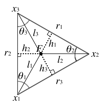
The simplest distance is then given by the sum of interquark distances in Eq. (15),

Another possible distance is given by the minimal total length of lines connecting the three quarks via the Fermat-Torricelli point of a triangle,

where $S$ is the area of the triangle given by Heron’s formula,

Note that the distance between the Fermat-Torricelli point and each vertex is

For finding the location of the Fermat-Torricelli point the method presented in [34, 35] may be useful.

In fact, these two types of distances, $\Delta$ and $Y$, were often used to examine the behavior of the potential in the earlier studies. We also follow them in our analyses of the three-quark potential. In terms of the minimal length of connected lines, $Y$ is reduced to

when $\theta_{\rm max}\geqq 120^{\circ}$. It is then convenient to introduce a combined distance of $Y$ and $\Lambda$ classified by $\theta_{\rm max}$ as

For a detailed comparison with the quark-antiquark potential, we also use a reduced interquark distance $R$ defined by

and an averaged distance between the Fermat-Torricelli point and three sides of a triangle (see, Fig. 4),

where

Note that $S_{i}=(1/2)l_{j}l_{k}\sin 120^{\circ}$ is the area of the triangle spanned by three points $x_{j}$, $x_{k}$, and $F$.

As we will see in the next section, these distances are quite useful to see the systematic behaviors of the three-quark potential, although it may be possible to define other symmetric distances [16].

At the beginning, we demonstrate that the three-quark potential can be obtained from one gauge configuration by tuning the parameters of the multilevel algorithm as explained in Sec. II.2. In Fig. 5, we plot typical convergence histories of the PLCF for the equilateral triangle configurations of one gauge configuration at $\beta=5.85$ ($N_{\rm tsl}=3$), $\beta=6.00$ ($N_{\rm tsl}=4$), and $\beta=6.30$ ($N_{\rm tsl}=6$) as a function of the number of internal updates $N_{\rm iupd}$. We find that the fluctuation of the PLCF is washed out and the values become stable as we increase $N_{\rm iupd}$. Required $N_{\rm iupd}$ for convergence depends on the size of the triangle.

Once the PLCF becomes stable, it can be regarded as the expectation value as in Eq. (13), and then the potential is computed by Eq. (8). In Fig. 6, we show the potential at $\beta=6.00$ from one gauge configuration at $N_{\rm iupd}=500000$ as a function of $Y$ defined in Eq. (17). The potential is also compared to that from the average of $N_{\rm cnf}=9$ independent gauge configurations (the number 9 is just the maximum gauge configurations that we obtained within our available computer resources). The numerical error of the average is estimated by the standard jackknife method. It is obvious that the potential is determined accurately, where the potential from one gauge configuration already represents the average. The level of agreement between the two potentials can be quantified by evaluating the relative error $(V^{\rm(ave)}_{3q}-V_{3q})/V^{\rm(ave)}_{3q}$, which is plotted in Fig. 7. This figure shows that the relative error is gradually increasing at large $Y$, which is one of the origin of the statistical error of the average. However it is only 0.8 % even at a quite long distance $Y/a\simeq 18$.

The fit of the averaged potential to an empirical functional form,

yields $A_{3q}^{\rm(Y)}=0.662(6)$, $\sigma_{3q}a^{2}=0.0446(3)$, and $\mu_{3q}a=1.092(3)$, which describes the behavior of the data nicely as shown in Fig. 6. It is interesting to note that the coefficient in front of $Y$, which we may call the three-quark string tension $\sigma_{3q}$, is consistent with the string tension of the quark-antiquark potential $\sigma_{{q\bar{q}}}$. In addition, the constant term $\mu_{3q}$ is approximately $(3/2)\mu_{{q\bar{q}}}$, where $\mu_{{q\bar{q}}}$ is the constant term of the quark-antiquark potential (discussed later in Sec. III.5).

We then extend the computation of the potential to various three-quark geometries as in Fig. 3 by using the same one gauge configuration at $\beta=6.00$. In total we investigate 221 three-quark geometries as summarized in Table 2. We list all of these potential data within the significant digits in Appendix A.

In Fig. 8, we plot all the potential data against $\Delta$ and $L_{\rm str}$ defined in Eqs. (16) and (21). At glance, we find that neither $\Delta$ nor $L_{\rm str}$ can provide a universal functional form of the three-quark potential, since all the data do not fall into one curve with these distances. However, if we look at the potential of ACT, RGT, and OBTN against $L_{\rm str}$ carefully and restrict the data only for $r_{\rm min}/a>2$, where $r_{\rm min}=\min(r_{1},r_{2},r_{3})$, by assuming that they do not suffer from severe lattice cutoff effects, we observe an excellent linearly-rising behavior as explicitly shown in Fig. 9. As we will demonstrate in the following analysis, the corresponding string tension is consistent with that of the quark-antiquark potential.

The behavior of the potentials of OBTW and LIN is not as clear as that of ACT and RGT. They are not on a simple function of $L_{\rm str}$. In particular, as explicitly shown in Fig. 10 for LIN, the potentials are dependent also on $r_{\rm min}$. The increasing behaviors as a function of $r_{\rm min}$ are similar with each other, which in turn imply that the three quarks in LIN prefers to be QDQ. As clarified later in Sec. III.4, the potential for LIN is well described by the half of the sum of the quark-antiquark potential, so that the interval between the potentials for various $L_{\rm str}$ in Fig. 10 is approximately given by $\sigma_{{q\bar{q}}}\delta L_{\rm str}$, where $\delta L_{\rm str}$ is the difference of $L_{\rm str}$.

The potential of QDQ exhibits a different behavior from that of other three-quark geometries. In Fig. 11, we plot the QDQ potential (we have selected only on-axis data), which is then compared to the quark-antiquark potential with the same distance between a quark and an antiquark $r$ (the raw data of the quark-antiquark potential are summarized in Table 11 in Appendix B). It appears that the two potentials are almost the same. Fitting the two potentials to the functional form,

leads to the values $A_{qdq}=0.336(2)$, $\sigma_{qdq}a^{2}=0.0449(1)$, and $\mu_{qdq}a=0.811(1)$ for the QDQ potential²² 2 The errors of the QDQ data, which are absent because of ${\displaystyle N_{\rm cnf}\!=\!1}$, are estimated from the residuals in the fitting process, and are used to evaluate the errors of the fit parameters., while $A_{{q\bar{q}}}=0.340(2)$, $\sigma_{{q\bar{q}}}a^{2}=0.0449(2)$, and $\mu_{{q\bar{q}}}a=0.766(1)$ for the quark-antiquark potential (see, Table 12 in Appendix B), where subscripts are added to distinguish the fit results; two potentials are consistent with each other except for the constant shift, $a(\mu_{qdq}-\mu_{{q\bar{q}}})=0.045(3)$.

We also compute the derivatives of the QDQ and the quark-antiquark potentials with respect to $r$, which are shown in Fig. 12. We find that the two results completely agree with each other, including a systematic effect caused by finite volume. These results mean that reduction of the representation in SU(3) color group, ${\bf 3}\otimes(\bar{\bf 3}\oplus{\bf 6})\Rightarrow{\bf 3}\otimes\bar{\bf 3}$, is realized nonperturbatively. Note that a similar result is obtained in Ref. [37] by using the $T$-shaped three-quark Wilson loop, where the distance between the two quarks for the diquark is set to two lattice steps.

The analysis in Sec. III.2 indicates that all of the three-quark potentials of various three-quark geometries cannot be parametrized by a unique distance simultaneously. However, if we look at the three-quark potential plotted in Fig. 8 optimistically, especially the plot against $L_{\rm str}$, there seems to be a common increasing behavior with different constant shifts. This may probably be due to the fact that somehow a common type of flux tube is formed among three quarks to minimize the total energy of the three-quark system, while the difference of the constants originates only from short distance effects among the three quarks, which persists even if one of the three quarks is located at a distance. We thus investigate the derivative of the potential with respect to $L_{\rm str}$ so that the short distance effects can be removed from the potential.

Let us first focus on the potential of the isosceles triangle geometries within ACT, where the two of three quarks are placed at $\vec{x}_{1}=(x,0,0)$ and $\vec{x}_{2}=(0,x,0)$, and the remaining third quark is placed at $\vec{x}_{3}=(0,0,z)$ with $z\geqq x$. In this case, $L_{\rm str}$ is identical to $Y$ and the distance between the Fermat-Torricelli point and $\vec{x}_{1}$ and $\vec{x}_{2}$, respectively, is the same $l_{1}=l_{2}=(\sqrt{6}/3)x$ (see, Fig. 4). Therefore, pulling the third quark (changing $z$) with the fixed first and second quarks does not affect the location of the Fermat-Torricelli point, which just affects the increase of the energy between the Fermat-Torricelli point and the third quark, where $l_{3}=\sqrt{z^{2}+x^{2}/2}-x/\sqrt{6}$. We then compute the derivative of the potential with respect to $Y$ for several fixed values of $x$,

In Fig. 13 (upper), we plot the result for one gauge configuration at $\beta=6.00$ with the classification in terms of the distance between the first and second quarks, $r_{\rm min}=\sqrt{2}\,x$, where $x/a=1$, $2$, and $3$ (in this case, $\delta Y=\delta l_{3}$). We find that all the derivatives behave quite similarly and approach a constant value at long distance. Remarkably, the constant value is nothing but the string tension in the quark-antiquark system, $\sigma_{{q\bar{q}}}a^{2}=0.0449$ (see, Table 12). Since the third quark is chosen arbitrarily among the three, this result also supports a picture of the $Y$-shaped flux-tube formation. This feature agrees with that was pointed out by Takahashi et al. [5, 6] based on the $\chi^{2}$ fit to the potential data with the $Y$ Ansatz.

We then pay attention to the potentials of RGT, where $\vec{x}_{2}=(0,y,0)$ and $\vec{x}_{3}=(0,0,0)$, and the remaining first quark is placed at $\vec{x}_{1}=(x,0,0)$, where $x\geqq y$. In this case, although the location of the Fermat-Torricelli point is slightly dependent on changing $x$, it becomes insensitive to $x$ when $x\gg y$. The derivative is then defined by

In Fig. 13 (middle), we plot the result for the same one gauge configuration with the classification in terms of the distance between the second and third quarks, $r_{\rm min}=y$, where $y/a=1\sim 4$. We find that all the derivatives approach the constant value, $\sigma_{{q\bar{q}}}a^{2}=0.0449$, at long distance: the tendency is quite the same as that for ACT.

We finally examine the potentials of LIN, where $\vec{x}_{1}=(x_{1},0,0)$, $\vec{x}_{2}=(x_{2},0,0)$, and $\vec{x}_{3}=(0,0,0)$, which is an extreme case that there is probably no chance to form a junction of the flux tube. For a fixed distance $r_{\rm min}=x_{2}$ ($0<x_{2}<x_{1}/2$), the derivative is then defined by

In Fig. 13 (bottom), we plot the result for the same one gauge configuration as a function of $L_{\rm str}=x_{1}$. We again find that all the derivatives approach the constant value, $\sigma_{{q\bar{q}}}a^{2}=0.0449$, at long distance.

These results strongly indicate that the energy of the flux tube per unit length, the string tension, is common to that of the quark-antiquark potential regardless of the geometry of three quarks.

In the earlier studies of the three-quark potential, there was a claim that the potential was described by the half of the sum of two-body potentials in the quark-antiquark system [4, 7]. However, our results in Sec. III.3, indicating the presence of the flux-tube junction in larger ACT and RGT, clearly contradict the earlier claim. Thus we critically compare the three-quark potential with the quark-antiquark potential. In fact, this is possible only when the both potentials are determined accurately up to long distance, otherwise one cannot distinguish the difference between them since it is not so apparent in practice as we will see below.

In Fig. 15, we plot the relative error between the three-quark potential and the half of the sum of the quark-antiquark potentials at $\beta=6.00$,

against $\Delta$ defined in Eq. (16), where we have selected only 55 three-quark geometries out of 221 ones. The selection is to perform the subtraction in Eq. (30) by using only the available raw data of the quark-antiquark potential as summarized in Tables 11 and 13 in Appendix B. We have avoided the use of the fit function of the quark-antiquark potential in Eq. (26), which may cause unwanted systematic effects especially at short distance.

We observe that the relative error is almost constant about 0.003 at $\Delta/a<10$, which may be understood as zero within the systematic error due to the use of different gauge configurations,³³ 3 Note, however, that our further analysis using exactly the same $N_{\rm cnf}=200$ gauge configurations for the three-quark and the quark-antiquark potentials at $\beta=6.00$ with $N_{\rm iupd}=10000$ indicates that this constant still remains finite about 0.002, which may be due to lattice cutoff effects. These potentials are not presented in this paper as the number of geometries is very limited, but the data are available on request. where the three-quark potential is from one gauge configuration with $N_{\rm iupd}=500000$, while the quark-antiquark potential is from $N_{\rm cnf}=20$ gauge configurations with $N_{\rm iupd}=100000$. On the other hand, the difference becomes apparent at $\Delta/a>10$ especially for ACT and RGT, both of which show a similar increasing behavior up to 0.03 at $\Delta/a=35$. Note that the relative error 0.03 is already large enough compared to that from the gauge configuration dependence as demonstrated in Fig. 7. In Fig. 15, we also plot the same relative error in Eq. (30) against $\theta_{\rm max}$ defined in Eq. (14). Clearly, some of ACT and RGT data (correspond to larger $\Delta$) exhibit a large deviation from zero.

The above two results seem to indicate that the large deviation in ACT and RGT originates from the formation of the flux-tube junction, since only these configurations are possible to form a proper junction at larger triangle. On the other hand, even in ACT and RGT, the flux-tube junction cannot be formed properly when the size of the triangle is insufficient. It seems that there is a critical size of the triangle to form a proper flux-tube junction. Based on this expectation, in Fig. 16, we then plot the relative error in Eq. (30) against the distance $h$ defined in Eq. (23), the averaged distance between the Fermat-Torricelli point and three sides of a triangle. Note that $h=0$ for LIN, while $h>0$ for the other triangles. We find that the relative errors of all the three-quark potential are well parametrized by $h$. The dashed line corresponds to a fit curve for the ACT data, which is an empirical quadratic function given by

where $c_{0}=0.0029(3)$, $c_{1}=-0.0011(7)$, and $c_{2}=0.0026(3)$. The relative errors seem to start increasing around $h/a\sim 0.6$.

The difference between the three-quark potential and the half of the sum of the quark-antiquark potentials signals an existence of three-body force among the three quarks. Our results in this subsection indicate that the difference is not so drastic when the size of the triangle is small or $\theta_{\rm max}$ approaches 180^∘, while it shows up gradually for larger ACT and RGT. In other words, it seems that the emergence of the three-body effects depends on whether the interquark distance among three quarks is large enough to form a flux-tube junction inside the triangle.

The analysis in Sec. III.3 suggests that the long distance part of the three-quark potential can be described by the term $\sigma_{3q}L_{\rm str}$, where the coefficient $\sigma_{3q}$ is common to that of the quark-antiquark potential $\sigma_{{q\bar{q}}}$. In addition, a naive fit result of the three-quark potential of the equilateral triangle geometries in Sec. III.1 as well as the analysis in Sec. III.4 have indicated that the potential also contains a constant term, which is approximately $3/2$ of that in the quark-antiquark potential $\mu_{{q\bar{q}}}$. The presence of such a constant term in the three-quark potential is quite natural in terms of the self-energy of quarks, which will be proportional to the number of quarks involved in the system.

We then investigate the behavior of the rest of the potential by subtracting the confinement term $\sigma_{{q\bar{q}}}L_{\rm str}$ and an expected constant term $(3/2)\mu_{{q\bar{q}}}$ from the three-quark potential,

which will be useful to clarify the short distance part of the potential. In Fig. 17, we plot Eq. (32) against $R$ defined in Eq. (22), where the three-quark potential used in this analysis is the same as that used in the previous subsections at $\beta=6.00$. From the quark-antiquark potential we take the values $\sigma_{{q\bar{q}}}a^{2}=0.0449(2)$ and $\mu_{{q\bar{q}}}a=0.766(1)$ (see, Table 12 in Appendix B). Remarkably, we find two systematic curves:⁴⁴ 4 Although we attempted to plot $V_{3q}^{\rm(sub.1)}$ with $\Delta$ and $L_{\rm str}$, we failed to see any systematic behaviors. one is mostly for LIN and the other is for triangle geometries although both seem to overlap at $R/a<1$. The data of LIN are well described by a function $-A_{{q\bar{q}}}/(2R)$ (the dotted line in the figure), where $A_{{q\bar{q}}}=0.340(2)$ is also from Table 12, which may not be surprising after the analysis in Sec. III.4. Since $L_{\rm str}=\Delta/2$ for LIN, the difference of the potential from the half of the sum of the quark-antiquark potential is at most 0.3 % relative error as explicitly shown in Fig. 15. What we should pay attention to is then the behavior of the other data for triangle geometries, which clearly deviates from the function $-A_{{q\bar{q}}}/(2R)$. Moreover, it seems that the curve approaches a negative constant value at large $R$. We then perform an empirical $\chi^{2}$ fit to the functional form,

which yields $A_{3q}^{\rm(R)}=0.126(3)$ and $\tilde{\mu}_{3q}a=-0.062(4)$ with $\chi^{2}/N_{\rm df}=0.04$, where the averaged potential of the equilateral triangle configuration with error bars is taken into account in the fit. It turns out that Eq. (33) nicely captures the increasing behavior of $V_{3q}^{\rm(sub.1)}$ (the dashed line in the figure). We find that $A_{3q}^{\rm(R)}$ is significantly smaller than $A_{{q\bar{q}}}/2=0.170$ about 26 %, namely,

and $\tilde{\mu}_{3q}$ has a negative value as expected. The value $0.259$ may be further tuned by performing a more sophisticated fit. The absolute value of $\tilde{\mu}_{3q}$ is one order of magnitude smaller than $\mu_{{q\bar{q}}}$, but still seems to be finite.

One may suspect at this stage that the existence of $\tilde{\mu}_{3q}$ just reflects a lattice artifact at $\beta=6.00$, however, the following analysis in Sec. III.6 shows a kind of scaling behavior on $\tilde{\mu}_{3q}$, which implies that $\tilde{\mu}_{3q}$ reflects a physical effect. Since the negative shift of the energy at large $R$ appears only for triangle geometries, we speculate that it just represents an energy reduction due to formation of the flux-tube junction. Of course, if this is the case, the energy reduction could depend on the size of the triangle. This feature seems to be incorporated effectively by rewriting Eq. (33) as

where the first term purely represents two-body interaction between quarks while the terms inside parenthesis are interpreted as the three-body junction effect. In Fig. 18, we plot

against $R$. Although it is not obvious in Fig. 17 whether OBTW belongs to LIN or triangle category, the plot in Fig. 18 seems to support the latter. The change of sign from positive to negative values around $R/a\sim 0.7$ may reflect the fact that forming a simple $Y$-shaped junction is rather costly for these smaller $R$, implying that a different type of flux structure is realized. It would be quite interesting to investigate the energy density of various three-quark systems with the PLCF.

To summarize, the functional form of the three-quark potential for triangle geometries is effectively parametrized by

On the other hand, the functional form for LIN can be described by the half of the sum of the quark-antiquark potential,

up to the tiny 0.3 % relative error as shown in Sec. III.4. We cannot answer here whether or not both functional forms can change continuously depending on the movement of quarks, which should be clarified in future study. It is certainly important for this purpose to see the potential of OBTW at long distance in detail. The functional form in Eq. (37) may be similar to that proposed by Takahashi et al. [5, 6] for triangle geometries, where the potential was parametrized by ${\displaystyle V_{3q}=-A_{{q\bar{q}}}/(2R)+\sigma_{{q\bar{q}}}Y+{\it constant}}$. However, our result shows a noticeable difference from it in terms of the junction term in Eq. (35).

So far we have concentrated on analyzing the potential at $\beta=6.00$, and have found the possible functional form of the potential as in Eqs. (37) and (38). We finally examine whether the functional form is still valid even if the lattice spacing decreases or increases. We then computed the three-quark potential at $\beta=5.85$ and $6.30$. We only pay attention to the potential of equilateral triangle geometries because of the limited computer resources, however, it will provide some hints concerning the scaling behavior of the potential. The number of gauge configurations to compute the final expectation values are not so many, but the statistical errors are highly suppressed by employing the multilevel algorithm with the tuned parameters, where $N_{\rm cnf}=8$ at $\beta=5.85$ with $N_{\rm iupd}=500000$, and $N_{\rm cnf}=6$ at $\beta=6.30$ with $N_{\rm iupd}=400000$. Typical convergence histories of the PLCF of the equilateral triangle geometry at $\beta=5.85$ and $\beta=6.30$ are already shown in Fig. 5.

In Fig. 20, we plot the potential as a function of $Y$, where physical scales are introduced according to Table 1 (the raw data and the fit results are summarized in Tables 9 and 10). In addition, the constant term $(3/2)\mu_{{q\bar{q}}}\,a$ is subtracted before we introduce the physical scale for each $\beta$ value. The constant term $\mu_{{q\bar{q}}}$ is extracted from the quark-antiquark potential as summarized in Table 12, which reflects the self-energy of a quark and an antiquark, and diverges in the continuum limit $a\to 0$. We find that the potential beautifully falls into one curve,

indicating a scaling behavior with respect to the lattice spacing.⁵⁵ 5 When we put three quarks at $(x,0,0)$, $(0,x,0)$, and $(0,0,x)$, the distance between the two of three quarks is $r=\sqrt{2}x$ and $Y=\sqrt{6}r=2\sqrt{3}x$. On the other hand, $R=\sqrt{2}x/3$, and then $R=\sqrt{3}Y/9=0.19245Y$. Thus, the function $1/Y$ and $1/R$ is the same for equilateral triangles up to a multiplicative factor. The quark-antiquark potential used in this analysis also exhibits a good scaling behavior as shown in Fig. 20 (the raw data and the fit results are summarized in Tables 11 and 12 in Appendix B). Comparison of the potentials at various $\beta$ values may be affected by the way of subtraction of the constant $\mu_{3q}$. This uncertainty can however be avoided by looking at the derivative of the potential with respect to $Y$, which is independent of the constant $\mu_{3q}$. The result is plotted in Fig. 21 and the data fall into a curve given by the derivative of Eq. (39) with respect to $Y$.

References

- [1] R. Sommer and J. Wosiek, Baryonic loops and the confinement in the three quark channel, Phys. Lett. B149, 497 (1984).
- [2] R. Sommer and J. Wosiek, Baryonic strings on a lattice, Nucl. Phys. B267, 531 (1986).
- [3] H. Thacker, E. Eichten, and J. Sexton, The three-body potential for heavy quark baryons in lattice QCD, Nucl. Phys. Proc. Suppl. 4, 234 (1988).
- [4] G. S. Bali, QCD forces and heavy quark bound states, Phys. Rept. 343, 1 (2001), eprint hep-ph/0001312.
- [5] T. T. Takahashi, H. Matsufuru, Y. Nemoto, and H. Suganuma, Three quark potential in the SU(3) lattice QCD, Phys. Rev. Lett. 86, 18 (2001), eprint hep-lat/0006005.
- [6] T. T. Takahashi, H. Suganuma, Y. Nemoto, and H. Matsufuru, Detailed analysis of the three quark potential in SU(3) lattice QCD, Phys. Rev. D 65, 114509 (2002), eprint hep-lat/0204011.
- [7] C. Alexandrou, Ph. de Forcrand, and A. Tsapalis, Static three quark SU(3) and four quark SU(4) potentials, Phys. Rev. D 65, 054503 (2002), eprint hep-lat/0107006.
- [8] C. Alexandrou, Ph. de Forcrand, and O. Jahn, The Ground state of three quarks, Nucl. Phys. Proc. Suppl. 119, 667 (2003), eprint hep-lat/0209062.
- [9] S. Kamizawa, Y. Matsubara, H. Shiba, and T. Suzuki, A static baryon in a dual Abelian effective theory of QCD, Nucl. Phys. B389, 563 (1993).
- [10] Y. Koma, E.-M. Ilgenfritz, T. Suzuki, and H. Toki, Weyl symmetric representation of hadronic flux tubes in the dual Ginzburg-Landau theory, Phys. Rev. D 64, 014015 (2001), eprint hep-ph/0011165.
- [11] H. Ichie, V. Bornyakov, T. Streuer, and G. Schierholz, The flux distribution of the three quark system in SU(3), Nucl. Phys. Proc. Suppl. 119, 751 (2003), eprint hep-lat/0212024.
- [12] V. G. Bornyakov, H. Ichie, Y. Mori, D. Pleiter, M. I. Polikarpov, G. Schierholz, T. Streuer, H. Stüben, and T. Suzuki (DIK), Baryonic flux in quenched and two flavor dynamical QCD, Phys. Rev. D 70, 054506 (2004), eprint hep-lat/0401026.
- [13] V. G. Bornyakov, M. N. Chernodub, H. Ichie, Y. Koma, Y. Mori, M. I. Polikarpov, G. Schierholz, H. Stüben, and T. Suzuki, Profiles of the broken string in two flavor QCD below and above the finite temperature transition, Prog. Theor. Phys. 112, 307 (2004), eprint hep-lat/0401027.
- [14] F. Bissey, F.-G. Cao, A. R. Kitson, A. I. Signal, D. B. Leinweber, B. G. Lasscock, and A. G. Williams, Gluon flux-tube distribution and linear confinement in baryons, Phys. Rev. D 76, 114512 (2007), eprint hep-lat/0606016.
- [15] M. Caselle, G. Delfino, P. Grinza, O. Jahn, and N. Magnoli, Potts correlators and the static three-quark potential, J. Stat. Mech. 0603, P03008 (2006), eprint hep-th/0511168.
- [16] V. Dmitrašinović, T. Sato, and M. Šuvakov, Smooth cross-over transition from the -string to the -string three-quark potential, Phys. Rev. D 80, 054501 (2009), eprint arXiv:0908.2687.
- [17] O. Andreev, Model of the -quark potential in gauge theory using gauge-string duality, Phys. Lett. B756, 6 (2016), eprint arXiv:1505.01067.
- [18] O. Andreev, Some aspects of three-quark potentials, Phys. Rev. D 93, 105014 (2016), eprint arXiv:1511.03484.
- [19] N. Brambilla, J. Ghiglieri, and A. Vairo, Three-quark static potential in perturbation theory, Phys. Rev. D 81, 054031 (2010), eprint arXiv:0911.3541.
- [20] N. Brambilla, F. Karbstein, and A. Vairo, Symmetries of the three-heavy-quark system and the color-singlet static energy at next-to-next-to-leading logarithmic order, Phys. Rev. D 87(7), 074014 (2013), eprint arXiv:1301.3013.
- [21] O. Kaczmarek, F. Karsch, E. Laermann, and M. Lutgemeier, Heavy quark potentials in quenched QCD at high temperature, Phys. Rev. D 62, 034021 (2000), eprint hep-lat/9908010.
- [22] N. Cardoso and P. Bicudo, Lattice QCD computation of the SU(3) string tension critical curve, Phys. Rev. D 85, 077501 (2012), eprint arXiv:1111.1317.
- [23] M. Lüscher and P. Weisz, Locality and exponential error reduction in numerical lattice gauge theory, JHEP 09, 010 (2001), eprint hep-lat/0108014.
- [24] M. Lüscher and P. Weisz, Quark confinement and the bosonic string, JHEP 07, 049 (2002), eprint hep-lat/0207003.
- [25] Y. Koma and M. Koma, The static three-quark potential from the Polyakov loop correlation function, PoS LATTICE2014, 352 (2014).
- [26] Y. Koma and M. Koma, The static potential from the selected intermediate states of gluons, PoS LATTICE2013, 469 (2013).
- [27] O. Jahn and O. Philipsen, Polyakov loop and its relation to static quark potentials and free energies, Phys. Rev. D 70, 074504 (2004), eprint hep-lat/0407042.
- [28] M. Koma and Y. Koma, The static three-quark potential of various quark configurations, PoS LATTICE2015, 324 (2016).
- [29] T. T. Takahashi and H. Suganuma, Detailed analysis of the gluonic excitation in the three-quark system in lattice QCD, Phys. Rev. D 70, 074506 (2004), eprint hep-lat/0409105.
- [30] M. Albanese, F. Costantini, G. G. Fiorentini, F. Flore, M. Lombardo, and R. Tripiccione (APE Collaboration), Glueball masses and string tension in lattice QCD, Phys. Lett. B192, 163 (1987).
- [31] Y. Koma, M. Koma, and H. Wittig, Nonperturbative determination of the QCD potential at O(1/m), Phys. Rev. Lett. 97, 122003 (2006), eprint hep-lat/0607009.
- [32] Y. Koma and M. Koma, Spin-dependent potentials from lattice QCD, Nucl. Phys. B769, 79 (2007), eprint hep-lat/0609078.
- [33] Y. Koma and M. Koma, Scaling study of the relativistic corrections to the static potential, PoS LAT2009, 122 (2009), eprint arXiv:0911.3204.
- [34] P. Bicudo and M. Cardoso, Iterative method to compute the Fermat points and Fermat distances of multiquarks, Phys. Lett. B674, 98 (2009), eprint arXiv:0812.0777.
- [35] C. Ay, J.-M. Richard, and J. H. Rubinstein, Stability of asymmetric tetraquarks in the minimal-path linear potential, Phys. Lett. B674, 227 (2009), eprint arXiv:0901.3022.
- [36] S. Necco and R. Sommer, The heavy quark potential from short to intermediate distances, Nucl. Phys. B622, 328 (2002), eprint hep-lat/0108008.
- [37] F. Bissey, A. Signal, and D. Leinweber, Comparison of gluon flux-tube distributions for quark-diquark and quark-antiquark hadrons, Phys. Rev. D 80, 114506 (2009), eprint arXiv:0910.0958.
- [38] A. S. Bakry, X. Chen, and P.-M. Zhang, Y-stringlike behavior of a static baryon at finite temperature, Phys. Rev. D 91, 114506 (2015), eprint arXiv:1412.3568.
- [39] A. S. Bakry, D. B. Leinweber, and A. G. Williams, Gluonic profile of the static baryon at finite temperature, Phys. Rev. D 91, 094512 (2015), eprint arXiv:1107.0150.