Finite element procedures for computing normals and mean curvature on triangulated surfaces and their use for mesh refinement

We define the tangential surface gradient $\nabla_{\Sigma}$ by $\nabla_{\Sigma}:=\bm{P}_{\Sigma}\nabla$, where $\nabla$ is the $\mathbb{R}^{3}$ gradient and $\bm{P}_{\Sigma}(\bm{x})=\bm{I}-\bm{n}(\bm{x})\otimes\bm{n}(\bm{x})$ is the projection onto the tangent plane $T_{\Sigma}(\bm{x})$ of $\Sigma$ at point $\bm{x}\in\Sigma$. The mean curvature vector $\bm{H}:\Sigma\rightarrow\mathbb{R}$ is then defined by

where $\bm{x}_{\Sigma}:\Sigma\ni\bm{x}\mapsto\bm{x}\in\mathbb{R}^{3}$ is the coordinate map of $\Sigma$ into $\mathbb{R}^{3}$ and $\Delta_{\Sigma}=\nabla_{\Sigma}\cdot\nabla_{\Sigma}$ is the Laplace–Beltrami operator.

The relation between the mean curvature vector and mean curvature is given by the identity

where $\kappa_{1}$ and $\kappa_{2}$ are the two principal curvatures and $(\kappa_{1}+\kappa_{2})/2=:H$ is the mean curvature, see [4].

The mean curvature vector satisfies the following weak problem: find $\bm{H}\in W=[H^{1}(\Sigma)]^{3}$ such that

where $\nabla_{\Sigma}\bm{w}=\bm{w}\otimes\nabla_{\Sigma}$ for a vector valued function $\bm{w}$ and

is the $L^{2}$–inner product on the set $\omega$ with associated norm

Given the discrete coordinate map $\bm{x}_{\Sigma_{h}}:\Sigma_{h}\ni\bm{x}\mapsto\bm{x}\in\mathbb{R}^{3}$ and a discrete projection operator $\bm{P}_{\Sigma_{h}}=\bm{I}-\bm{n}_{h}\otimes\bm{n}_{n}$, where $\boldsymbol{n}_{h}$ denotes the piecewise constant facet normals, we define the stabilized discrete mean curvature vector $\bm{H}_{h}$ as follows. Let $V_{h}$ be the space of piecewise linear continuous functions defined on $\mathcal{K}_{h}$ and seek $\bm{H}_{h}\in W_{h}=[V_{h}]^{3}$ such that

where $\nabla_{\Sigma_{h}}=\bm{P}_{\Sigma_{h}}\nabla$ and the stabilization term $J_{h}(\cdot,\cdot)$ is defined by

Here $\gamma\geq 0$ is a stabilization parameter and $\mathcal{E}_{h}=\{E\}$ is the set of edges in the partition $\mathcal{K}_{h}$ of $\Sigma_{h}$. The jump of the tangential derivative in the direction of the outer co-normals at an edge $E\in\mathcal{E}_{h}$ shared by elements $K_{1}$ and $K_{2}$ in $\mathcal{K}_{h}$ is defined by

where $u_{i}=u|_{K_{i}}$, $i=1,2,$ and $\bm{t}_{E,K_{i}}$ are the co-normals, i.e., the unit vectors orthogonal to $E$, tangent and exterior to $K_{i}$, $i=1,2$, see Figure 1. This stabilization method allows for proving first order convergence of the curvature vector $\|\bm{H}-\bm{H}_{h}^{l}\|_{\Sigma}\lesssim h,$ see [13].

Using the standard Galerkin approximation,

where $\varphi_{i}$ is the finite element basis functions and $U_{i}$ the nodal approximations of $u$ we have that

were we define the tangential gradient of the basis function by

The tangential derivative of the basis function is given by

For vector–valued unknowns $\bm{u}$ we have $\bm{u}\approx\bm{\Phi}{\mathbf{u}}$ where ${\mathbf{u}}$ denotes nodal values and

and using the notation $\bm{t}_{1}$ and $\bm{t}_{2}$ for the two co-normals on a given edge $E$, we define

and the discrete stabilization matrix is given by

The linear system corresponding to (6) becomes

where ${\mathbf{M}}$ is the so called mass matrix, given by

$\gamma_{H}$ is the mean curvature specific stabilization factor, ${\mathbf{S}}$ is the discrete Laplace-Beltrami operator defined by

with

${\mathbf{x}}$ is the coordinate vector of the nodal positions in the mesh, and ${\mathbf{H}}$ denotes the vector of vertex values of the approximate mean curvature vector.

There exists several well known approaches to mean curvature estimation, for an extensive overview, see [18]. In the context of finite elements an alternative to ours is proposed by Heine in [14].

We shall compare our method to two types of such approaches: 1) fitting a surface locally to each vertex, see e.g., [1, Chap. 8.5] and 2) computing the discrete local Laplace-Beltrami operator, see e.g., [21, 8].

Smooth surface fit. Curvatures can be computed using a locally fitted quadratic function

around a point ${\mathbf{x}_{i}}$ with $u$ and $v$ are local coordinates of the tangential plane to ${\mathbf{x}_{i}}$ such that $f(0,0)=0$. The tangential plane is determined using one of the edges connected to ${\mathbf{x}_{i}}$ and the normal at the same point. The idea is to compute the shape operator or Weingarten map of this function and subsequently the curvature. See [1, Chap. 8.5] for further details.

The discrete local Laplace-Beltrami operator. Let ${\mathbf{K}}$ denote the Laplace–Beltrami operator so that ${\mathbf{K}}(\bm{x})=2H(\bm{x})\bm{n}(\bm{x})$ at a given point $\bm{x}$ on the surface. On triangulated surfaces, one can use Gauss’ theorem to extract a discrete version of this operator in the nodes ${\mathbf{x}_{i}}$ of the mesh, cf. Meyer et al. [21]. The integral of ${\mathbf{K}}$ over the discrete 1-ring surface M on a triangulated surface is then given by

where the angles $\alpha_{ij}$ and $\beta_{ij}$ are opposite to the edge $i\ j$ and $N$ is the set of neighbour vertices to ${\mathbf{x}_{i}}$, see Figure 2a. Given some definition $A_{V}$ of the local area surrounding a vertex ${\mathbf{x}_{i}}$ we can then define the discrete approximation ${\mathbf{K}}_{h}$ of ${\mathbf{K}}$ as

In [21], it is proposed to use the Voroni regions as the definition for the local area, and an algorithm to improve the robustness for arbitrary meshes was provided. Similarly, Desbrun et. al [8] used the barycentric area to average the discrete Laplacian. In both cases, in order to compute the vertex normal, ${\mathbf{K}_{h}({\mathbf{x}_{i})}}$ is simply normalized and cases where the curvature is zero are treated by computing the mean face-normal of the 1-ring neighbourhood. The mean (discrete) curvature at the vertices is then given by

In analogy with (6) we define the recovered discrete normal vector $\bm{n}_{h}$ as follows: find $\bm{n}_{h}\in W_{h}=[V_{h}]^{3}$ such that

where $\bm{n}_{K}$ is the piecewise constant exterior normal to the facet elements $K$. The corresponding linear system becomes

where $\gamma_{n}$ is the normal-specific stabilization factor, ${\mathbf{n}}_{h}$ the vector of vertex normals, and

Note that (12) can be efficiently solved using a conjugate gradient method since ${\mathbf{M}}$ is symmetric, positive definite and sparse.

When translating the computed normal vector field to a set of discrete vertex normals, these will here be normalized (the nodal vectors contained in ${\mathbf{n}}_{h}$ are not in general of unit length).

Traditionally, vertex normals are estimated either from a local neighborhood of surrounding face normals using some type of local averaging, see e.g., [17, 23] and the references therein. Other estimation methodologies also exists such as local smooth surface fits, see, e. g., [20]. We use the notations for the local vertex normals introduced in [23] and give a brief description; see Figure 2b for an explanation of the notations used.

Mean weighted equally. Arguably, the most widespread estimation of the vertex normal was introduced by Gouraud [12] as

where $\bm{n}_{i}$ is the face-normal of triangle $i$ , $n$ is the total number of triangles that share a common vertex for which the vertex normal is to be estimated and $|.|$ denotes the norm. Note that we shall subsequently omit making the normalization step of the vertex normal explicit and assume $\bm{n}=\hat{\bm{n}}:=\bm{n}/|\bm{n}|$.

Mean weighted by angle. A vertex normal approximation using angles between the inner edges was proposed by Thürrner and Wüthrich [27].

where $\alpha_{i}$ is the angle between two edges $\bm{e}_{k}$ and $\bm{e}_{k+1}$ of a face $i$ sharing the vertex.

Mean weighted by sine and edge length reciprocals. Max [19] proposed several methods of weighting the face normals, one of which is to weight by the sine and edge length reciprocals to take into account the difference in lengths of surrounding edges.

Mean weighted by areas of adjacent triangles. Another method proposed by Max [19] is to weight the normals by the area of the face.

where the symbol $\times$ denotes the vector cross product.

Mean weighted by edge length reciprocals. Max [19] also proposed to just use the edge length reciprocals as weights.

Mean weighted by square root of edge length reciprocals. Finally, Max [19] also suggested to use the square root of the length reciprocals.

Normal from the discretized local Laplace-Beltrami operator. Another approach is to define the normal using the discretized local Laplace-Beltrami operator (DLLB) defined in Section 3.3. The normal is defined by normalizing the discrete mean curvature vector.

In the numerical example below, Section 6, we compare the accuracy of these different approaches.

We base our adaptive algorithm on the Zienkiewicz–Zhu approach [30] which employs the difference between recovered derivatives and actual discrete piecewise derivatives of a finite element solution. By analogy we consider the piecewise constant normals to play the role of the piecewise derivatives, and compare these to the $L^{2}-$projected normals.

Since we are focusing on vertex normals, and since we will in the following compare methods that only produce such normals, we define a norm which is an approximation of the $L^{2}$–norm,

where $\text{meas}(K)$ denotes the area of $K$ and $\boldsymbol{x}^{i}_{K}$ the vertex coordinates on $K$. This represents a Newton–Cotes numerical integration scheme for the $L^{2}(\Sigma_{h})$–norm using the vertices as integration points. The error in normals is thus approximated

and we aim at achieving

where TOL is a given tolerance. We note that we also have

where $h$ is the local mesh size and $\nabla_{\Sigma}\bm{n}$ is the curvature tensor, which indicates that we counter large curvature by reduced mesh size for resolution of the geometry.

In cases where the exact geometry is not accessible, we consider triangle refinement approaches that utilise vertex normals for interpolation. An overview of such methods is given by Boschiroli et al. in [3]. Nagata [22] proposed a simple quadratic interpolation of triangles using vertex normals and positions at the end-nodes. The approach by Nagata depends on a curvature parameter that fixes a curvature coefficient in order to stabilize the method. The curvature coefficient is highly dependent on the vertex normal, and in cases where normals are near parallel, the method cannot capture inflections and without a stabilizing parameter, cusps will be introduced to the surface, see [23] where the authors point out this problem and suggest a possible solution. The solution suggested in [23] eliminates the problem of cusps in the interpolated surface but also eliminates the inflection, since the segment becomes linear. Another approach is to use higher order interpolation which are able to capture inflection points.

Since the PN refinement with $N=1$ splits the face of a flat triangle into four child elements, we need a way of handling the hanging nodes. In this work we adapt the Red-Green refinement method proposed by Banks et al in [2]. This method preserves the aspect ratio of the initial mesh which is crucial in order to secure the accuracy of the associated finite element method.

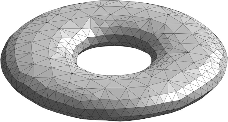
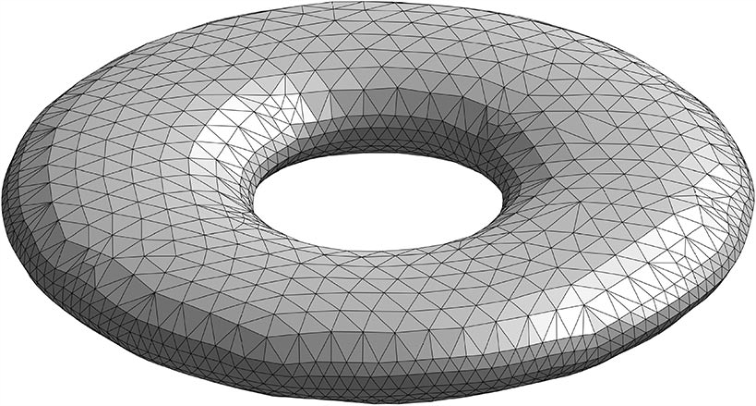
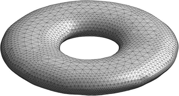
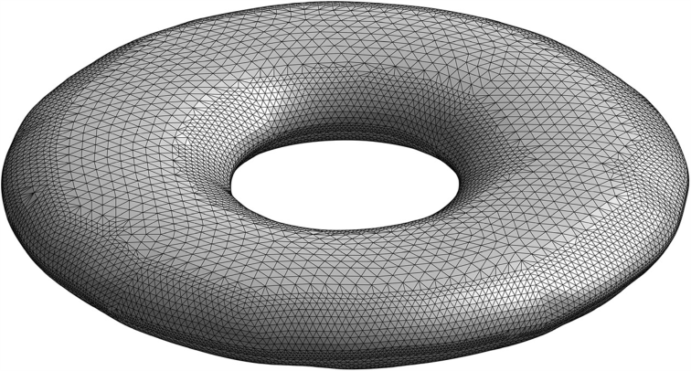
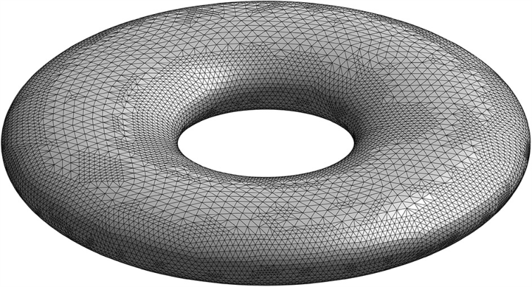
We choose to analyze the errors on an implicitly defined torus which we can modify in order to generate slightly more complex features. The surface equation for the torus is given by

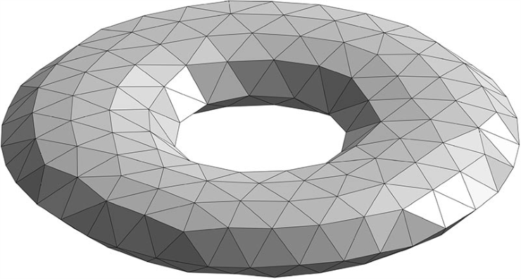
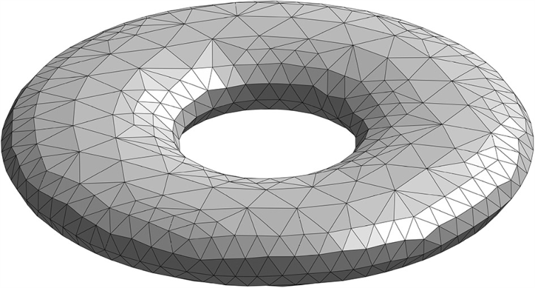
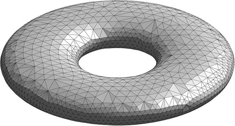
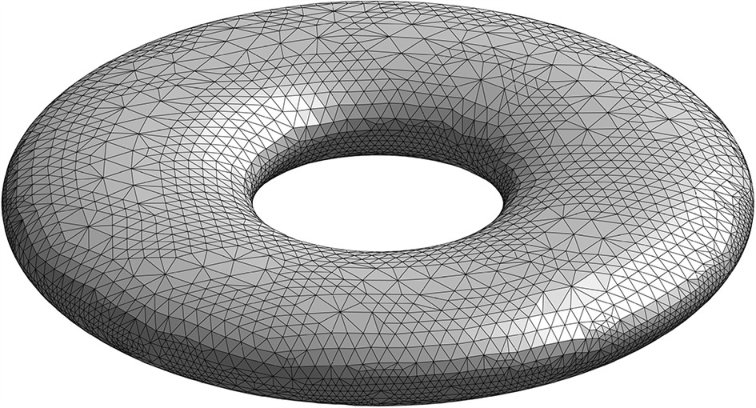
where $R$ is the torus radius, $r$ the tube radius and $a$ is a “squish-factor” used to squish the torus in the z-direction in order to induce a higher curvature on the inside and outside, see Figure 6. In the following, the torus will be analyzed with $a=1$ and $a=4$, in order to compare errors with respect to strongly and smoothly varying curvature.

What follows is a comparison of different vertex normals with the exact normal. The measure for the mesh-size used in this context is defined as

where $N_{\text{v}}$ denotes the number of vertices in the mesh.

Using an implicitly defined surface $\Sigma=\{\bm{x}:\phi(\bm{x})=0\}$, where $\phi$ is a signed distance function with the property $|\nabla\phi|=1,$ we have that $\bm{n}(\bm{x}_{\Sigma})=\nabla\phi(\bm{x}_{\Sigma})$. As discussed above, we will use (20) and define the error as

where $\bm{n}_{a}$ is the approximate and $\bm{n}_{e}$ the exact normal defined by $\bm{n}_{e}=\nabla\phi$, computed at the vertex $i$ using $\bm{n}_{e}^{i}=\nabla\phi(\bm{x}^{i})$. The convergence rates are defined as

The vertex normal error analysis was done on an unstructured mesh of a torus with $R=1$, and $r=1/2$ and $a=\{1,4\}$, see Figure 6.

The convergence of $L^{2}$ errors $\epsilon$ defined in (34) are shown in Figure 7 were it can be seen that the stabilized $L^{2}$–projection of the normals converges optimally. The raw data for this graph is available in Table 1. The relative difference between the stabilized $L^{2}$ normals and the next best traditional method $\bm{n}_{\mathrm{MWA}}$ can be seen in Table 2 where we can see a relative error decrease from $\epsilon_{\text{MWA}}$ of $\sim 29\%$ to $\sim 88\%$ depending on mesh-size and geometry. The convergence rates can be viewed in Table 3. In the next section we shall analyze the impact of the stabilization on the normal errors.

In this section we analyze the influence of the stabilization factor on the vertex normal error numerically by employing a golden search method to find the optimal stabilization factor $\gamma_{n}^{*}$ that minimizes the normal error $\epsilon$ defined in (34).

where we use $\gamma_{n}^{0}=0$ and $\gamma_{n}^{1}=1$. This is done for several mesh-sizes and on a torus with $a=1$ and $a=4$, see Figure 8 and 9. Notice how the curves become more planar, i.e., choosing a “good” $\gamma_{n}$ becomes less sensitive with the decrease in $h$.

The error difference is shown in Figure 10 and Table 4 where $\epsilon_{L^{2}}$ is the $L^{2}$ error, defined in (34), of the $L^{2}$ vertex normals without stabilization and $\epsilon_{L_{\mathrm{stab}}^{2}}$ is the error of the stabilized $L^{2}$ vertex normal which is stabilized with a optimal stabilization factor $\gamma^{*}$.

In a 2D case we can see in Figure 11 how the choice of vertex normals affects the resulting cubic interpolation. The initial mesh is coarse and the (unstabilized) $L^{2}$–projected normals are not just depending on the nearest neighbors to each vertex but globally. The resulting difference is apparent.

We compare the impact of different vertex normals on the interpolation by measuring the geometrical error defined as

where $\bm{x}_{\Sigma}(\bm{n})$ denotes the discrete surface interpolated with a particular normal approximation method. We measure the $L^{2}_{h}$–norm of the signed distance. The refinement algorithm employed is the PN triangles using 1 tessellation per face see Figure 5. The mesh-size in this section is defined as

where $N_{\text{e}}$ denotes the number of elements and $A_{K}$ is the area of the $K$-th element. The initial mesh-size is $h=0.1618$ and the initial $L^{2}_{h}$–norm of the signed distance error is $\epsilon_{\mathrm{geom}}=0.0863$. See Figure 12 for the convergence comparison, Table 5 for the regular refinement data and Table 6 for the local refinement data.

Examples of interpolation using PN triangles with local refinement are shown in Figure 13 for the Torus, Figure 14 for the Utah teapot and Figure 15 for the Stanford bunny.

The local refinement method is compared to local refinement with projection to the exact surface, see Figure 16. We compare the approximite normal error with the exact normal error by computing the effectivity index, given by

where $\bm{n}_{e}$ is the exact normal to the surface, $\bm{n}_{f}$ is the face normal and $\bm{n}_{L^{2}_{\mathrm{stab}}}$ is the recovered stabilized $L^{2}$–projected normal, see Table 7.

The mean curvature is computed on a structured and unstructured torus with $R=1$, $r=1/2$ and $a=1$. We compare the mean curvature approximation to the exact mean curvature, the smooth surface fit approach (SSF) and the discrete local Laplace-Beltrami (DLLB) approach described in Section 3.3, and our stabilized discrete curvature vector solving (10). In the last case we compute the mean curvature $H_{h}$ through

where $\bm{n}_{h}$ denotes the normal computed using the stabilized $L^{2}$–projection from (12). In our computational experience, this gives a more accurate result than the immediate $H_{h}=\frac{1}{2}|\bm{H}_{h}|$.

In Figure 17 we give iso-plots of the mean curvature. Figure 18 shows the convergence of mean curvature.

References

- [1] J. A. Bærentzen, J. Gravesen, F. Anton, and H. Aanæs. Guide to computational geometry processing: foundations, algorithms, and methods. Springer Science & Business Media, 2012.
- [2] R. E. Bank, A. H. Sherman, and A. Weiser. Some refinement algorithms and data structures for regular local mesh refinement. Sci. Comput. Appl. Math. Comput. Phys. Sci, 1:3–17, 1983.
- [3] M. Boschiroli, C. Fünfzig, L. Romani, and G. Albrecht. A comparison of local parametric Bézier interpolants for triangular meshes. Comput. Graph., 35(1):20–34, 2011.
- [4] M. Botsch, L. Kobbelt, M. Pauly, P. Alliez, and B. Lévy. Polygon Mesh Processing. A. K. Peters, Ltd., Natick, MA, 2010.
- [5] M. Botsch and O. Sorkine. On linear variational surface deformation methods. IEEE Trans. Vis. Comput. Graph., 14(1):213–230, 2008.
- [6] M. Cenanovic, P. Hansbo, and M. G. Larson. Minimal surface computation using a finite element method on an embedded surface. Int. J. Numer. Meth. Engng, 104(7):502–512, 2015.
- [7] A. Demlow. Higher order finite element methods and pointwise error estimates for elliptic problems on surfaces. SIAM J. Numer. Anal., 47(2):805–827, 2009.
- [8] M. Desbrun, M. Meyer, P. Schröder, and A. H. Barr. Implicit fairing of irregular meshes using diffusion and curvature flow. In Proceedings of the 26th Annual Conference on Computer Graphics and Interactive Techniques, SIGGRAPH ’99, pages 317–324, New York, NY, USA, 1999. ACM Press/Addison-Wesley Publishing Co.
- [9] G. Dziuk. Finite elements for the Beltrami operator on arbitrary surfaces. In Partial differential equations and calculus of variations, volume 1357 of Lecture Notes in Math., pages 142–155. Springer, Berlin, 1988.
- [10] G. Dziuk. An algorithm for evolutionary surfaces. Numer. Math., 58(6):603–611, 1991.
- [11] G. Dziuk. Computational parametric Willmore flow. Numer. Math., 111(1):55–80, 2008.
- [12] H. Gouraud. Continuous shading of curved surfaces. IEEE Trans. Comput., 100(6):623–629, 1971.
- [13] P. Hansbo, M. G. Larson, and S. Zahedi. Stabilized finite element approximation of the mean curvature vector on closed surfaces. SIAM J. Numer. Anal., 53(4):1806–1832, 2015.
- [14] C.-J. Heine. Isoparametric finite element approximation of curvature on hypersurfaces. Citeseer, 2004.
- [15] C.-J. Heine. Computations of form and stability of rotating drops with finite elements. IMA J. Numer. Anal., 26(4):723–751, 2006.
- [16] K. Hildebrandt and K. Polthier. Anisotropic filtering of non-linear surface features. Comput. Graph. Forum, 23(3):391–400, 2004.
- [17] S. Jin, R. R. Lewis, and D. West. A comparison of algorithms for vertex normal computation. Vis. Comput., 21(1-2):71–82, 2005.
- [18] E. Magid, O. Soldea, and E. Rivlin. A comparison of Gaussian and mean curvature estimation methods on triangular meshes of range image data. Comput. Vis. Image Underst., 107(3):139–159, 2007.
- [19] N. Max. Weights for computing vertex normals from facet normals. Journal of Graphics Tools, 4(2):1–6, 1999.
- [20] D. S. Meek and D. J. Walton. On surface normal and Gaussian curvature approximations given data sampled from a smooth surface. Comput. Aided Geom. Design, 17(6):521–543, 2000.
- [21] M. Meyer, M. Desbrun, P. Schröder, and A. H. Barr. Discrete differential-geometry operators for triangulated 2-manifolds. In Visualization and mathematics III, Math. Vis., pages 35–57. Springer, Berlin, 2003.
- [22] T. Nagata. Simple local interpolation of surfaces using normal vectors. Comput. Aided Geom. Design, 22(4):327–347, 2005.
- [23] D. M. Neto, M. C. Oliveira, L. F. Menezes, and J. L. Alves. Improving Nagata patch interpolation applied for tool surface description in sheet metal forming simulation. Comput. Aided Des., 45(3):639–656, 2013.
- [24] B. T. Phong. Illumination for computer generated pictures. Commun. ACM, 18(6):311–317, 1975.
- [25] A. Schmidt. Computation of three dimensional dendrites with finite elements. J. Comput. Phys., 125(2):293–312, 1996.
- [26] V. Surazhsky and C. Gotsman. Explicit surface remeshing. In Proceedings of the 2003 Eurographics/ACM SIGGRAPH symposium on Geometry processing, pages 20–30. Eurographics Association, 2003.
- [27] G. Thürmer and C. A. Wüthrich. Computing vertex normals from polygonal facets. J. Graph. Tools, 3(1):43–46, 1998.
- [28] A. Vlachos, J. Peters, C. Boyd, and J. L. Mitchell. Curved PN triangles. In Proceedings of the 2001 symposium on Interactive 3D graphics, pages 159–166. ACM, 2001.
- [29] G. Xu. Consistent approximations of several geometric differential operators and their convergence. Appl. Numer. Math., 69:1–12, 2013.
- [30] O. C. Zienkiewicz and J. Z. Zhu. A simple error estimator and adaptive procedure for practical engineering analysis. Internat. J. Numer. Methods Engrg., 24(2):337–357, 1987.