Distributed Mechanism Design with Learning Guarantees

There are $K$ infinitely divisible goods, denoted by set $\mathcal{K}=\{1,\ldots,K\}$, that are to be distributed among the agents. Each agent receives a utility $v_{i}(x_{i})$ based on the profile $x_{i}=(x_{i}^{1},\ldots,x_{i}^{K})$ of quantity of each good that he/she receives. Since for each agent, its utility depends only on privately consumed allocation $x_{i}$ and not on other agents’ allocation, this is the private goods model.

It is assumed that $v_{i}:\mathbb{R}^{K}\rightarrow\mathbb{R}$ is a continuously double-differentiable, strictly concave function that satisfies, $\forall~k\in\mathcal{K}$,

for any given $\eta>1$, where $H^{-1}$ is the inverse of the Hessian $H=\left[\left.(\partial^{2}v_{i}(\cdot))\middle/(\partial x_{i}^{k}\partial x_{i}^{l})\right.\right]_{k,l}$. To understand the significance of this assumption consider the case of $K=1$, then this condition is the same as

It is already assumed that $v_{i}(\cdot)$ is strictly concave, the only additional imposition made by this assumption is that the second derivative of $v_{i}(\cdot)$ is strictly bounded away from $0$ and $-\infty$. More generally if the utility is separable, $v_{i}(x_{i})=\sum_{k\in\mathcal{K}}v_{i,k}(x_{i}^{k})$, then the condition in (1) is the same as

The above mentioned properties of the utility function are assumed to be common knowledge between agents and the designer. However, the utility function $v_{i}(\cdot)$ itself is known only to agent $i$ and is not known to other agents or the designer. The designer wishes to allocate available goods such that the sum of utilities is maximized subject to availability constraints, i.e., to solve the following centralized allocation problem,

where $c_{k}\in\mathbb{R}$ is the total available amount of good $k\in\mathcal{K}$. The allocation $x^{*}$ is also called the efficient allocation and it is assumed to be finite i.e., the optimization is well-defined. The efficient allocation is unique since the utilities are strictly concave. Further, the necessary and sufficient condition for optimality are

where $\big(\lambda_{k}^{*}\big)_{k\in\mathcal{K}}\in\mathbb{R}^{K}$ are the (unique) optimal dual variables for each constraint in (4b).

There is a single infinitely divisible public good with $P$ features, with the set of features denoted by $\mathcal{P}=\{1,\ldots,P\}$. Each agent receives a utility $v_{i}(x)$ based on the quantity of the public good $x=\left(x^{p}\right)_{p\in\mathcal{P}}\in\mathbb{R}^{P}$. Since for each agent, its utility depends on the common allocation $x$, this is the public goods model. It is assumed that $v_{i}:\mathbb{R}^{P}\rightarrow\mathbb{R}$ is a continuously double-differentiable, strictly concave function that satisfies (1) with the Hessian $H=\left[\left.(\partial^{2}v_{i}(\cdot))\middle/(\partial x^{p}\partial x^{q})\right.\right]_{p,q}$. If $P=1$, then this condition is the same as in (2). As in the private goods model, the properties of the utility function are assumed to be common knowledge between agents and the designer. However, the utility function $v_{i}(\cdot)$ itself is known only to agent $i$ and is not known to other agents or the designer. The designer wishes to allocate the public good such that the sum of utilities is maximized, i.e., to solve the following centralized allocation problem,

The allocation $x^{*}$ is also called the efficient allocation and it is assumed to be finite i.e., the optimization is well-defined. The efficient allocation is unique due to strictly concave utilities. The necessary and sufficient optimality conditions can be written as

where $\big({\mu_{i}^{p}}^{*}\big)_{p\in\mathcal{P},i\in\mathcal{N}}$ are the (unique) optimal dual variables.

In general, for the public goods problem one can also assume a seller in the system who produces the quantity $x$ and for whom the cost of production is a known (convex) function. In this case, the social welfare maximizing allocation contains the utility of the seller as well. For keeping exposition clear and to focus on the similarities between the public and private goods problems, the seller is not considered in this model. If needed, this can accommodated in a straightforward manner.

In the next two sections, we present a mechanism for each of the above problems.

A one-shot mechanism is defined by the triplet,

which consists of, for each agent $i\in\mathcal{N}$, the message space $\mathcal{M}_{i}$, the allocation function $\widehat{x}_{i}:\mathcal{M}\rightarrow\mathbb{R}^{K}$ and the tax function $\widehat{t}_{i}:\mathcal{M}\rightarrow\mathbb{R}$. Given a mechanism, a game $\mathfrak{G}_{pvt}$ is setup between the agents in $\mathcal{N}$, with action space $\mathcal{M}$ and utilities

For this game, $\widetilde{m}\in\mathcal{M}$ is a Nash equilibrium if

The mechanism is said to fully implement the efficient allocation if

where $\mathcal{M}_{NE}\subseteq\mathcal{M}$ is the set of all Nash equilibria of game $\mathfrak{G}_{pvt}$ and $x^{*}$ is the efficient allocation from (4). Furthermore, the mechanism is said to be budget balanced at Nash equilibrium if

Finally, we call the mechanism distributed if for any agent $i\in\mathcal{N}$, the allocation function $\widehat{x}_{i}(\cdot)$ and tax function $\widehat{t}_{i}(\cdot)$ instead of depending on the entire message $m=(m_{j})_{j\in\mathcal{N}}$, depend only on $m_{i}$ and $\big(m_{j}\big)_{j\in\mathcal{N}(i)}$, i.e., agent $i$ and his/her immediate neighbors. Here $\mathcal{N}(i)$ are all the “out”-neighbors of $i$ i.e., there exists an edge from $i$ to $j$ in graph $\mathcal{G}$ iff $j\in\mathcal{N}(i)$ .

For the purpose of maintaining clarity in the exposition, the mechanism presented below is for the special case of a single private good i.e., $K=1$. A natural extension of the presented mechanism to the general case is discussed at the end of this section.

For any agent $i\in\mathcal{N}$, the message space is $\mathcal{M}_{i}=\mathbb{R}^{N+1}$. The message $m_{i}=(y_{i},q_{i})$ consists of agent $i$’s demand $y_{i}\in\mathbb{R}$ for the allocation of the single good and a surrogate/proxy $q_{i}=\left(q_{i}^{1},\ldots,q_{i}^{N}\right)\in\mathbb{R}^{N}$ for the demand of all the agents (including himself/herself).

Since the underlying graph $\mathcal{G}=\left(\mathcal{N},\mathcal{E}\right)$ is strongly connected, for any pair of vertexes $i,j\in\mathcal{N}$, the following two quantities are well-defined. $d(i,j)$ is the length of the shortest path from $i$ to $j$ and $n(i,j)\in\mathcal{N}(i)$ is the out-neighbor of $i$ such that the shortest path from $i$ to $j$ goes through $n(i,j)$. The two quantities are depicted in Fig. 1. The allocation function is defined as

where $\xi\in(0,1)$ is an appropriately chosen contraction parameter and its selection is discussed in Section 5 on Learning Guarantees, proof of Proposition 3. The tax function is defined as

where $n(i,i)\in\mathcal{N}(i)$ is an arbitrarily chosen neighbor of $i$ and $\delta>0$ is an appropriately chosen parameter. Both $\xi,\delta$ are selected simultaneously in the proof of Proposition 3 from Section 5.

The quantities, $n(\cdot,\cdot)$ and $d(\cdot,\cdot)$, are based on the graph $\mathcal{G}$. The only property of relevance here is that the two are related recursively i.e., $d(n(i,r),r)=d(i,r)-1$. Thus if a mechanism designer wishes to avoid calculating the shortest path (possibly due to the high complexity) then $n,d$ can be replaced by any valid neighbor and distance mapping, respectively, as long as they are related recursively as above.

The distributed-ness of the mechanism follows from the fact that the expressions in (13) and (14) depend only on $m_{i}$ and $\big(m_{r}\big)_{r\in\mathcal{N}(i)}$.

Since agents are connected through a given graph, they can only communicate with a restricted set of agents i.e., their neighbors. Yet, as indicated in the optimality conditions, (5), there needs to be two kinds of global consensus at the efficient allocation. Firstly, the total allocation to all the agents must equal the total available amount, $\sum_{i\in\mathcal{N}}x_{i}^{*}=c_{1}$. Secondly, agents also need to agree on a common “price”, $\lambda_{1}^{*}$. To facilitate this, the message space consists of the surrogate variables $q_{i}=(q_{i}^{1},\ldots,q_{i}^{N})$ which are known locally to agent $i$ and are expected at equilibrium to be representative of the global demand $y=(y_{1},\ldots,y_{N})$. Specifically, the second, third and fourth terms in the tax, (14a), are designed for incentivizing agents to achieve the aforementioned duplication of global demand $y$ to the local surrogate $q_{i}$.

To motivate the choice of the allocation function and the remaining part of the tax function consider the case of $\xi=1$ and take into account the duplication, i.e., $q_{r}=y$, $\forall\>r\in\mathcal{N}$. Since $\xi=1$, all the factors involving $\xi$ become $1$ for the expressions in (13) and (14). We design the allocation $\widehat{x}_{i}(m)$ as a function of $y_{i}$ and $\left(q_{r}\right)_{r\in\mathcal{N}(i)}$ such that after taking into account the duplication it becomes $y_{i}-\frac{1}{N-1}\sum_{j\neq i}y_{j}+\frac{c_{1}}{N}$. This facilitates the first global consensus, $\sum_{i\in\mathcal{N}}x_{i}=c_{1}$. One standard design principle for mechanisms is that if an agent partially controls their own allocation (such as here, since $\widehat{x}_{i}(m)$ depends on $y_{i}$) then they shouldn’t be able to control the price. This is the reason that $\widehat{p}_{i}(\cdot)$ doesn’t depend on $m_{i}$. It is function of $\left(q_{r}\right)_{r\in\mathcal{N}(i)}$ and is designed such that after taking into account the duplication, the price for any agent is proportional to $\sum_{j}y_{j}$. This facilitates the second consensus - common price for all agents.

Finally, we set $\xi<1$ and adjust the allocation and tax function accordingly so that the game $\mathfrak{G}_{pvt}$ can be contractive (see Section 5).

Before proceeding to the main results, define the best-response of any agent $i$,

Denote $\beta=\left(\beta_{1},\ldots,\beta_{N}\right)$. Best-response $\beta:\mathcal{M}\rightarrow\mathcal{M}$ is a set-valued function in general.

Concavity of the induced utility in the game $\mathfrak{G}_{pvt}$ largely follows from the tax terms being quadratic. The second tax term in (14a) is the only source of cross derivatives across components of message $m_{i}$. Concavity is proved by verifying that the Hessian matrix is negative definite.

The proof of Proposition 1 can be intuitively explained as follows. Since the optimality conditions in (5) are sufficient, we start by showing that at any Nash equilibrium the allocation and price necessarily satisfy the optimality conditions. Thereby ensuring that if Nash equilibrium exists (unique or multiple) the corresponding allocation is efficient. Then we show existence and uniqueness by showing a one-to-one map between message at Nash equilibrium and $(x^{*},\lambda^{*})$ arising out of the optimization in (4).

The optimality conditions in (7) require that agents have global consensus on two aspects: allocation must be the same for all and sum of prices should be equal to zero. As in the private goods mechanism, we design the second, third and fourth tax terms in (22a) such that agents are incentivized to duplicate global demand $y$ onto locally available variables $q_{i}$. To motivate the allocation function and the remaining part of the tax function consider the case of $\xi=1$ and take into account the duplication $q_{r}=y$, $\forall~r\in\mathcal{N}$. In this case all the factors involving $\xi$ in (21) and (22) are 1. The allocation function $\widehat{x}_{i}(m)$ depends on $y_{i},\left(q_{r}\right)_{r\in\mathcal{N}(i)}$ and is designed such that after taking into account the duplication it is proportional to $\sum_{j}y_{j}$. This facilitates the first consensus - all agents’ allocation must be the same. The price $\widehat{p}_{i}(m_{-i})$ is designed such that it depends only on $\left(q_{r}\right)_{r\in\mathcal{N}(i)}$ and after taking into account the duplication it is proportional to $y_{i}-\frac{1}{N-1}\sum_{j\neq i}y_{j}$. This facilitates the second consensus - sum of prices over all agents is zero.

With the above design principles, all the results of this section follow. We then introduce an additional fifth term in the tax, (22a), just for the purpose of achieving contraction in Section 5 (see proof of Proposition 4). Incentives provided by this term are in line with those already provided to the neighboring agent $n(i,i)$ through his/her third tax term, hence it doesn’t interfere with the equilibrium results in this section. Only the proof of concavity changes slightly.

Finally, we set $\xi<1$ and adjust everything in the allocation and tax function correspondingly so that the game $\mathfrak{G}_{pub}$ can be contractive (see Section 5).

For the next two results, the basic idea behind the proofs are similar to the corresponding results from the previous section.

The intuition behind the proof of Proposition 3 can be motivated as follows. By selecting parameter $\xi<1$, contraction of best-response for the variables $\left(\tilde{q}_{i}^{r}\right)_{r\neq i}$ is already ensured. However, for best-response in $\tilde{y}_{i},\tilde{q}_{i}^{i}$, tuning of $\xi,\delta$ is needed. Due to the specific nature of the mechanism it turns out that in order to accommodate any given value of $\eta>1$, $\xi$ needs to be selected close to $1$ and correspondingly $\delta$ needs to be selected as a function of the chosen $\xi$. Finally, it is also shown that the best-response $\tilde{y}_{i}$ and $\tilde{q}_{i}^{i}$ are decreasing in $q_{n(i,i)}^{i}$ and hence the game is not supermodular.

For numerical analysis we consider the private goods problem with one good $(K=1)$ and the public goods problem with one feature $(P=1)$ and $N=31$, $\eta=25$. The agents’ utility function as quadratic, i.e.,

An example of quadratic utility function can be found in [28], for the model of demand side management in smart-grids. In each case the second derivative of $v_{i}(\cdot)$ is $2\theta_{i}$ and thus for any agent $i$ the value for $\theta_{i}$ is chosen uniformly randomly in the range $(-\frac{\eta}{2},-\frac{1}{2\eta})$. As the model doesn’t impose any restriction on the first derivative, the value for $\sigma_{i}$ is chosen uniformly randomly in the range $(10,20)$. From the proof of Propositions 3 and 4, one can numerically calculate the value of parameters $\xi,\delta$. For the particular instance of the random $\theta,\sigma$ generated to be used for the plots below (the same values for $\theta,\sigma$ are used for both public and private goods examples), the parameter values are listed in Table 1. The two cases for graph $\mathcal{G}$ considered are: a full binary tree and a sample of the Erdős-Reńyi random graph with only one connected component, where any two edges are connected with probability $p=0.3$. The first represents a case of small average degree whereas the second represents the case of large average degree. The same instance of Erdős-Reńyi random graph is used for both private and public goods examples.

Since it has been shown that the best-response is a contraction mapping, one expects that any learning strategy that best-responds to some convex combination of past actions from finitely many rounds, converges at an exponential rate. Indeed, this is exactly observed from Fig. 2 and 5, where the absolute distance $\|m_{n}-\widetilde{m}\|_{2}$ of the action in round $n$ to the Nash equilibrium $\widetilde{m}$ of the game $\mathfrak{G}_{pvt}$ and $\mathfrak{G}_{pub}$ is plotted versus $n$, respectively. For the learning dynamic⁰⁰ 0 A theoretical simplification with quadratic utilities $v_{i}(\cdot)$ is that for learning strategies such as $k-$period best-response or Fictitious Play, instead of maintaining the empirical distribution over other agents’ past actions, every agent can simply maintain the empirical average., one case considered is when the action taken by any agent $i$ at time $n$ is the best-response to an exponentially weighed average of past actions, i.e.,

The second learning dynamic is to best-respond to the average of past 10 rounds.

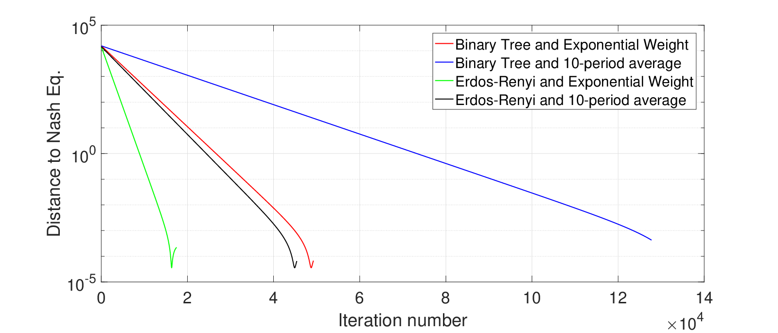
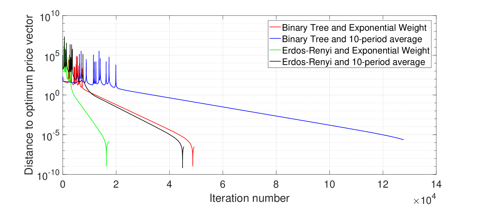
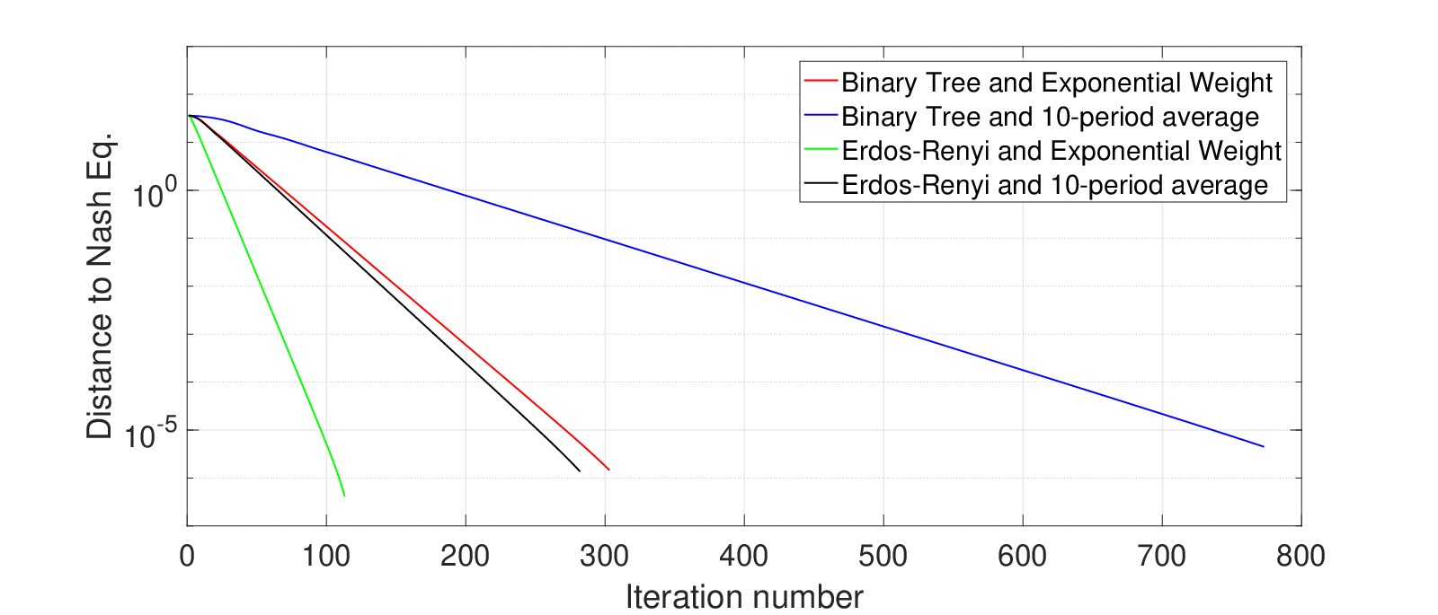
Since the learning iterations are essentially conducting information exchange, one expects that the convergence to be faster for a graph that is more connected. From both the figures this is evident, as for each learning dynamic higher average degree Erdős-Reńyi random graph shows faster convergence than lower average degree Binary Tree. In fact, for both learning dynamics the convergence for the Erdős-Reńyi random graph is faster than either learning dynamic for Binary Tree. Comparing the two learning dynamics among themselves, we observe that the more aggressive exponential weighing leads to faster convergence compared to the learning dynamic that puts equal weight on each of the previous 10 actions. Finally, for Fig. 2, in each case the relative distance to Nash equilibrium, defined as $\left.\|m_{n}-\widetilde{m}\|_{2}\middle/\|\widetilde{m}\|_{1}\right.$, is in the order of $10^{-9}$ when the absolute distance to Nash equilibrium is $10^{-3}$. For Fig. 5, the relative distance in each case is of the order of $10^{-8}$ when the absolute distance to Nash equilibrium is $10^{-5}$.

Fig. 3 and 4 refer to the private goods mechanism and plot the distance of allocation $\widehat{x}(m_{n})$ and price $\left(p_{1}(m_{n}),\ldots,p_{N}(m_{n})\right)$ in round $n$ to $x^{*}$ and $\left(\lambda_{1}^{*},\ldots,\lambda_{1}^{*}\right)$, respectively. The convergence pattern is the same as the one observed in Fig. 2, for the distance of message $m_{n}$ to Nash equilibrium $\widetilde{m}$.

References

- [1] Leonid Hurwicz and Stanley Reiter. Designing economic mechanisms. Cambridge University Press, 2006.
- [2] Rakesh V Vohra. Mechanism Design: a linear programming approach, volume 47. Cambridge University Press, 2011.
- [3] Tilman Borgers, Daniel Krahmer, and Roland Strausz. An introduction to the theory of mechanism design. Oxford University Press, 2015.
- [4] Frank P Kelly, Aman K Maulloo, and David KH Tan. Rate control for communication networks: shadow prices, proportional fairness and stability. Journal of the Operational Research society, 49(3):237–252, 1998.
- [5] Rajiv T Maheswaran and Tamer Başar. Social welfare of selfish agents: motivating efficiency for divisible resources. In 43rd IEEE Conference on Decision and Control, 2004. CDC., volume 2, pages 1550–1555. IEEE, 2004.
- [6] Sichao Yang and Bruce Hajek. VCG-Kelly mechanisms for allocation of divisible goods: Adapting VCG mechanisms to one-dimensional signals. IEEE Journal on Selected Areas in Communications, 25(6):1237–1243, 2007.
- [7] Ramesh Johari and John N Tsitsiklis. Efficiency of scalar-parameterized mechanisms. Operations Research, 57(4):823–839, 2009.
- [8] Rahul Jain and Jean Walrand. An efficient Nash-implementation mechanism for network resource allocation. Automatica, 46(8):1276–1283, 2010.
- [9] A. Kakhbod and D. Teneketzis. An efficient game form for unicast service provisioning. IEEE Transactions on Automatic Control, 57(2):392–404, 2012. ISSN 0018-9286.
- [10] Saptarshi Bhattacharya, Koushik Kar, Joe H Chow, and Aparna Gupta. Extended second price auctions with elastic supply for PEV charging in the smart grid. IEEE Transactions on Smart Grid, 7(4):2082–2093, 2016.
- [11] A. Sinha and A. Anastasopoulos. Mechanism design for resource allocation in networks with intergroup competition and intragroup sharing. IEEE Transactions on Control of Network Systems, PP(99):1–1, 2017. ISSN 2325-5870. 10.1109/TCNS.2017.2680319.
- [12] Angelia Nedić and Asuman Ozdaglar. Distributed subgradient methods for multi-agent optimization. IEEE Transactions on Automatic Control, 54(1):48–61, 2009.
- [13] Stephen Boyd, Neal Parikh, Eric Chu, Borja Peleato, and Jonathan Eckstein. Distributed optimization and statistical learning via the alternating direction method of multipliers. Foundations and Trends® in Machine Learning, 3(1):1–122, 2011.
- [14] John C Duchi, Alekh Agarwal, and Martin J Wainwright. Dual averaging for distributed optimization: Convergence analysis and network scaling. IEEE Transactions on Automatic control, 57(3):592–606, 2012.
- [15] Y. Sun, G. Scutari, and D. Palomar. Distributed nonconvex multiagent optimization over time-varying networks. In 2016 50th Asilomar Conference on Signals, Systems and Computers, pages 788–794, Nov 2016. 10.1109/ACSSC.2016.7869154.
- [16] Timothy Besley and Stephen Coate. Centralized versus decentralized provision of local public goods: a political economy approach. Journal of public economics, 87(12):2611–2637, 2003.
- [17] Shrutivandana Sharma and Demosthenis Teneketzis. Local public good provisioning in networks: A Nash implementation mechanism. IEEE Journal on Selected Areas in Communication, 30(11):2105–2116, 2012.
- [18] Paul Milgrom and John Roberts. Rationalizability, learning, and equilibrium in games with strategic complementarities. Econometrica: Journal of the Econometric Society, pages 1255–1277, 1990.
- [19] H Peyton Young. Strategic learning and its limits. Oxford University Press, 2004.
- [20] Drew Fudenberg. The theory of learning in games, volume 2. MIT press, 1998.
- [21] Martin J Osborne and Ariel Rubinstein. A course in game theory. MIT press, 1994.
- [22] Jonh F. Nash. Non-cooperative Games. PhD thesis, Princeton University, May 1950.
- [23] Yan Chen. A family of supermodular Nash mechanisms implementing Lindahl allocations. Economic Theory, 19(4):773–790, 2002.
- [24] Paul J Healy and Laurent Mathevet. Designing stable mechanisms for economic environments. Theoretical Economics, 7(3):609–661, 2012.
- [25] Leonid Hurwicz. Outcome functions yielding Walrasian and Lindahl allocations at Nash equilibrium points. The Review of Economic Studies, 46(2):217–225, 1979.
- [26] Andreu Mas-Colell, Michael Dennis Whinston, Jerry R Green, et al. Microeconomic theory, volume 1. Oxford university press New York, 1995.
- [27] George W Brown. Iterative solution of games by fictitious play. Activity analysis of production and allocation, 13(1):374–376, 1951.
- [28] P. Samadi, H. Mohsenian-Rad, R. Schober, and V. W. S. Won. Advanced demand side management for the future smart grid using mechanism design. IEEE Transactions on Smart Grid, 3(3):1170–1180, Sept 2012.
- [29] Abhinav Sinha and Achilleas Anastasopoulos. A general mechanism design methodology for social utility maximization with linear constraints. ACM SIGMETRICS Performance Evaluation Review, 42(3):12–15, 2014. 10.1145/2695533.2695538.
Appendix A Proof of Lemma 1 (Concavity - Private goods)
Proof.
Since the allocation and tax functions are smooth and is continuously double-differentiable, to establish concavity we show that the Hessian of w.r.t. is negative definite i.e., . Once this is established, the optimization in (15) has a strictly concave objective and an unbounded constraint set. Thus it has a unique maximizer, defined by the first order derivative conditions.
The Hessian is of size and we have