Occupation times for the finite buffer fluid queue
with phase-type ON-times
Abstract
In this short communication we study a fluid queue with a finite buffer. The performance measure we are interested in is the occupation time over a finite time period, i.e., the fraction of time the workload process is below some fixed target level. Using an alternating renewal sequence, we determine the double transform of the occupation time; the occupation time for the finite buffer M/G/1 queue with phase-type jumps follows as a limiting case.
Keywords:
Occupation time fluid model phase type distribution doubly reflected process finite buffer queue
Affiliations:
N. J. Starreveld is with Korteweg-de Vries Institute for Mathematics, Science Park 904, 1098 XH Amsterdam, University of Amsterdam, the Netherlands. Email: n.j.starreveld@uva.nl. R. Bekker is with Department of Mathematics, Vrije Universiteit Amsterdam, De Boelelaan 1081a, 1081 HV Amsterdam, The Netherlands. Email: r.bekker@vu.nl. M. Mandjes is with Korteweg-de Vries Institute for Mathematics, University of Amsterdam, Science Park 904, 1098 XH Amsterdam, the Netherlands; he is also affiliated with EURANDOM, Eindhoven University of Technology, Eindhoven, the Netherlands, and CWI, Amsterdam the Netherlands. Email: m.r.h.mandjes@uva.nl.
Mathematics Subject Classification:
60J55; 60J75; 60K25.
1 Introduction
Owing to their tractability, the OR literature predominantly focuses on queueing systems with an infinite buffer or storage capacity. In practical applications, however, we typically encounter systems with finite-buffer queues. Often, the infinite-buffer queue is used to approximate its finite-buffer counterpart, but it is questionable whether this is justified when the buffer is not so large.
In specific cases explicit analysis of the finite-buffer queue is possible. In this paper we consider the workload process of a fluid queue with finite workload capacity . Using the results for the fluid queue we also analyze the finite-buffer M/G/1 queue. The performance measure we are interested in is the so-called occupation time of the set up to time , for some , defined by
| (1.1) |
Our interest in the occupation time can be motivated as follows. The queueing literature mostly focuses on stationary performance measures (e.g. the distribution of the workload when ) or on the performance after a finite time (e.g. the distribution of at a fixed time ). Such metrics do not always provide operators with the right means to assess the service level agreed upon with their clients. Consider for instance a call center in which the service level is measured over intervals of several hours during the day; a typical service-level target is then that 80% of the calls should be answered within 20 seconds. Numerical results for this call center setting [16, 17] show that there is severe fluctuation in the service level, even when measured over periods of several hours up to a day. Using a stationary measure for the average performance over a finite period may thus be highly inadequate (unless the period over which is averaged is long enough). The fact that the service level fluctuates on such rather long time scales has been observed in the queueing community only relatively recently (see [5, 16, 17] for some call center and queueing applications). Our work is among the first attempts to study occupation times in finite-capacity queueing systems.
Whereas there is little literature on occupation times for queues, there is a substantial body of work on occupation times in a broader setting. One stream of research focuses on occupation times for processes whose paths can be decomposed into regenerative cycles [8, 18, 19, 20]. Another branch is concerned with occupation times of spectrally negative Lévy processes, see e.g. [14, 15, 13]. The results established typically concern occupation times until a first passage time, whereas [13] focuses on refracted Lévy processes. In [18] spectrally positive Lévy processes with reflection at the infimum were studied as a special case; we also refer to [18] and references therein for additional literature. A natural extension of Lévy processes are Markov-modulated Lévy processes; for the case of a Markov-modulated Brownian motion the occupation time has been analyzed in [7]. To the best of our knowledge there is no paper on occupation times for doubly reflected processes, as we consider here.
In this paper we use the framework studied in [18]. More specifically, the occupation time is cast in terms of an alternating renewal process, whereas for the current setting the upper reflecting barrier complicates the analysis. We consider a finite buffer fluid queue where during ON times the process increases linearly and during OFF times the process decreases linearly. We consider the case that ON times have a phase-type distribution and the OFF times have an exponential distribution. This framework allows us to exploit the regenerative structure of the workload process and provides the finite-capacity M/G/1 queue with phase-type jumps as a limiting special case. For this model we succeed in deriving closed-form results for the Laplace transform (with respect to ) of the occupation time. Relying on the ideas developed in [3], all quantities of interest can be explicitly computed as solutions of systems of linear equations.
The structure of the paper is as follows. In Section 2 we describe the model and give some preliminaries. Our results are presented in Section 3. A numerical implementation of our method is presented in Section 4.
2 Model description and preliminaries
We consider the finite capacity fluid queue with linear rates. The rate is determined by an independently evolving Markov chain, where we assume that there is only one state in which work decreases; this may be interpreted as the OFF time of a source that feeds work into the queue. There are multiple states of the underlying Markov chain during which work accumulates at (possibly) different linear rates. In case these rates are identical, periods during which work accumulates may be interpreted as ON times of a corresponding ON-OFF source. The ON-OFF source then has exponentially distributed OFF times, whereas the ON times follow a phase-type distribution. The workload capacity is and work that does not fit is lost; see Subsection 2.2 for a more formal description. Some basic results concerning phase-type distributions and martingales that are used in the sequel are first presented in Subsection 2.1.
2.1 Preliminaries
Phase-type distributions
A phase-type distribution is defined as the absorption time of a continuous-time Markov process with finite state space such that is an absorbing state and the states in are transient. We denote by the initial probability distribution of the Markov process, by the phase generator, i.e., the rate matrix between the transient states and by the exit vector, i.e., the - dimensional rate vector between the transient states and the absorbing state . The vector can be equivalently written as , where is a column vector of ones. We denote such a phase-type distribution by where . The cardinality of the state space , i.e., , represents the number of phases of the phase-type distribution ; for simplicity we assume that . In what follows we denote by a phase-type distribution with representation ; for a phase-type distribution with representation we add the subscript in the notation. An important property of the class of phase-type distributions is that it is dense (in the sense of weak convergence) in the set of all probability distributions on ; see [2, Thm. 4.2]. For a phase-type distribution with representation , the cumulative distribution function , the density and the Laplace transform are given in [2, Prop. 4.1]. In particular, for and , we have
| (2.1) |
When the phase-type distribution has representation we use the notation instead of . For a general overview of the theory of phase-type distributions we refer to [2, 3] and references therein.
Markov-additive fluid process (MAFP)
Markov-additive fluid processes belong to a more general class of processes called Markov-additive processes, see [2, Ch. XI]. Consider a right-continuous irreducible Markov process defined on a filtered probability space with a finite state space and rate transition matrix . While the Markov process is in state the process behaves like a linear drift . We assume that the rates are independent of the process . Letting be the jump epochs of the Markov process (with ) we obtain the following expression for the process ,
| (2.2) |
where and is independent of the Markov process and the rates . The process defined in (2.2) will be referred to as a Markov-additive fluid process and abbreviated as MAFP. For , the matrix exponent of the MAFP is defined as
| (2.3) |
In what follows we shall need information concerning the roots of the equation
| (2.4) |
where and . From [10] we have that there exist values and corresponding vectors such that, for each , and .
The Kella-Whitt martingale
The counterpart of the Kella-Whitt martingale for Markov-additive processes was established in [4]; let be an adapted continuous process having finite variation on compact intervals. Set and let . Then, for every initial distribution ,
| (2.5) |
is a vector-valued zero mean martingale.
2.2 Fluid model with two reflecting barriers
The MAFP we analyze has a modulating Markov process with state space and generator given by
| (2.6) |
which is a matrix. Additionally we suppose that , is a column vector with non-negative entries, is a column vector with entries that sum up to one and is a matrix with non-negative off-diagonal entries. The column vector and the matrix are such that each row of sums up to one, alternatively we can write . On the event the process decreases linearly with rate and on the event , for , increases linearly with rate . Such a MAFP decreases linearly with rate during OFF-times, which are exponentially distributed with parameter , and increases linearly with rates during ON-times, which have a phase-type distribution. Depending on the state of the modulating process we have a different rate. This model is motivated by finite capacity systems with an alternating source: during OFF times work is being served with rate while during ON times work accumulates with rates .
The workload process we are interested in is formally defined as a solution to a two sided Skorokhod problem, i.e., for a Markov-additive fluid process as defined in (2.2), we have
| (2.7) |
In the above expression represents the local time at the infimum and the local time at . Informally, for , is the amount that has to be added to so that it stays non-negative while is the amount that has to be subtracted from so that it stays below level . It is known that such a triplet exists and is unique, see [11, 12]. For more details we refer to [9] and references therein. For notational simplicity we assume that and that , i.e., we start with an OFF time; the cases and can be dealt with analogously at the expense of more complicated expressions. For the MAFP described above the matrix exponent is a matrix. For , denote by the roots of the equation and consider, for , the vectors defined by
| (2.8) |
where is the unit column vector with 1 at position , and are as in (2.6) and is the diagonal submatrix of with at position , for . For the vectors defined in (2.8) we have that for all .
3 Result
3.1 The Markov Additive Fluid Process
For the analysis of the occupation time we observe that the workload process alternates between the two sets and . Due to the definition of both upcrossings and downcrossings of level occur with equality. Moreover, we see that an upcrossing of level can occur only when the modulating Markov process is in one of the states . Similarly, a downcrossing of level can occur only while the modulating Markov process is in state 1. We define the following first passage times, for ,
We use the notation for the sequence of successive downcrossings and for the sequence of successive upcrossings of level . An extension of [8, Thms. 1 and 2] for the case of doubly reflected processes shows that is a renewal process, and hence the successive sojourn times, , , for , and , for , are sequences of well defined random variables. In addition, is independent of while in general and are dependent. We observe that the random vectors are i.i.d. and distributed as a generic random vector . In Figure 1 a realization of is depicted.
The double transform of the occupation time in terms of the joint transform of and is given in [18, Theorem 3.1] which we now restate:
Theorem 3.1.
For the transform of the occupation time , and for , we have
| (3.1) |
where, for ,
Remark 1.
To analyze the occupation time it thus suffices to determine the joint transform of the random variables and , i.e., . The Laplace transform of the random variables and have been derived in [6] for MAFPs. Our proofs can be trivially extended in order to derive the joint transform of the random variables and for a general MAFP, i.e. with multiple states with negative drifts, which is an additional novelty of this paper. Our interest lies though in the occupation time so we restrict ourselves to the MAFP considered in Section 2.2.
For we define the first hitting time of level with initial condition as follows:
Considering the event that an upcrossing of level occurs while the modulating process is in state , for , we obtain, for ,
| (3.2) |
In what follows we use, for and , the notation
| (3.3) |
It will be shown that these terms can be computed as the solution of a system of linear equations. The idea of conditioning on the phase when an upcrossing occurs and using the conditional independence of the corresponding time epochs has been developed in [3]. The factors appearing in each term in (3.3) can also be determined using the results of [6]. Determining the factors involved in the terms presented above is the main contribution of the analysis that follows. We first present the exact expression for the double transform of the random variables .
Theorem 3.2.
The outer sum in (3.4) ranging from 2 to represents the conditioning on one of the phases of the modulating Markov process when an upcrossing occurs, that is the event , . Observe that an upcrossing of level is not possible when is in state 1 because then the process decreases. The terms , as defined in (3.3), denote the transforms of on the event the upcrossing of level occurs while the modulating Markov process is in state , and the inner sum in (3.4) concerns the transforms of conditional on the event . The Markov property of the workload process yields that
| (3.5) |
Proof of Theorem 3.2.
The proof relies on the decomposition given in (3.2). Below we analyze the two expectations at the RHS of (3.2) separately.
We determine , for , as the solution of a system of linear equations; this idea was initially developed in [3, Section 5] and essentially relies on the Kella-Whitt martingale for Markov Additive Processes. The Kella-Whitt martingale for a Markov Additive Process reflected at the infimum, has, for all , and for , the following form
| (3.6) |
The expression above follows from the general form of the Kella-Whitt martingale given in (2.5) by considering the process defined by , for . This gives . The process has paths of bounded variation and is also continuous since the local time at the infimum is a continuous process. Hence, is a zero-mean martingale. Furthermore, due to the construction of the model we have that . Applying the optional sampling theorem for the stopping time , we obtain, for all ,
| (3.7) |
where
and
The row vector represents the local time at the infimum up to the stopping time ; the process can hit level 0 only on the event . Consider the roots of the equation , denoted by , and the corresponding column vectors , for as defined in (2.8). Substituting in (3.7) and taking the inner products with the column vectors we obtain, for , the system of equations
| (3.8) |
Solving this system of equations we obtain the , for .
Next, consider the second expectation in each of the summands at the RHS of (3.2), i.e., the term . This expectation represents the transform of the first time the process hits level given that , for . The Kella-Whitt martingale, for a MAFP reflected at , has, for all and for , the following form:
| (3.9) |
The expression above follows from the general form of the Kella-Whitt martingale given in (2.5) by considering the process defined by , for . This gives . A similar argument as for the stopping time and (3.5) yields systems of linear equations; for each , we solve for the unknowns and , , using the following system:
| (3.10) |
where . Using the method of determinants we can write in the following form:
| (3.11) |
where, for ,
3.2 The finite buffer queue
Using the result of Theorem 3.2 we can also study the occupation time of the workload process in a finite-buffer queue with phase-type service time distribution. Consider a queue where customers arrive according to a Poisson process with rate and have a phase-type service time distribution with representation . Moreover, the queue has finite capacity and work is served with rate . The workload process is modeled using a reflected compound Poisson process with negative drift and upward jumps with a phase-type distribution. Such a process has Laplace exponent equal to
| (3.14) |
where . As for the MAFP in Section 3.1 we determine the joint transform of the random variables and . First we introduce some notation. Define, for , the vectors as:
| (3.15) |
where are the roots of the equation . Consider the following system of linear equations
| (3.16) |
and define and as in (3.12) and (3.13) above with the defference that is replaced by .
Corollary 3.1.
Consider a compound Poisson process with negative drift and upward jumps with a phase-type distribution. Consider the process reflected at the infimum and at level . For , the joint transform of the random variables and is given by
| (3.17) |
where and are as above; for are determined as the solution of (3.16) and is as in (3.15).
The workload process can be studied as the limit of a MAFP in the following sense, see also [4, Section 7]. Following the construction presented in Section 2.2 we define, for , the MAFP where the Markov process has state space and generator given by
which is a matrix. We also let the positive rates be equal, i.e, and we send later on. The assumptions on and T are the same as in Section 2.2. On the event the process decreases with rate and on the event , for , the process increases with rate . Such a MAFP decreases linearly with rate during OFF-times, which are exponentially distributed with parameter and increases linearly with rate during ON-times, which have a phase-type distribution. By multiplying the matrix with the factor we see that the resulting phase-type distribution behaves like a phase-type distribution with representation divided by . Using the representation in (2.2) we see that letting the process converges path-wise to a compound Poisson process with linear rate and jumps in the upward direction with phase-type distribution. The workload process converges to , i.e. a reflected compound Poisson process, which follows by the continuity of the reflection operators with respect to the topology. Hence the joint transform of and is computed by using the result established in Theorem 3.2 and letting .
4 Numerical Computation
In this note we have studied the occupation time of the workload process of the set upto time for the finite buffer fluid queue with a single state (of an independently evolving Markov chain) in which the workload decreases. Special cases are ON-OFF sources where the OFF times are exponential and the ON-times follow a phase type distribution; the M/G/1 queue with phase-type jumps can be studied as a limiting special case. By considering the process , the results for fluid queues with a single state where work accumulates is now immediate; the same then holds for ON-OFF sources with phase-type OFF times and exponential ON times and doubly reflected risk reserve processes with negative phase-type jumps.
Essential in our analysis was the joint transform of the consecutive periods below and above , i.e., for . The double transform of the occupation time uniquely specifies its distribution, which can be evaluated by numerically inverting the double transform [1]. Such a procedure has been carried out in [16] for the M/M/ queue, where an explicit expression for the double transform can be derived. For the current model, the transform is given implicitly, where for given linear equations need to be solved. The methodology we present is rather straightforward to implement and yields an approximation for the distribution function of the occupation time up to machine precision. We first present an algorithm which uses Theorem 3.4 in order to numerically approximate the distribution function (or the density function) of the occupation time . Afterwards using the technique presented above we let and obtain the distribution function of the occupation time in the M/G/1 queue with phase-type service distribution.
Algorithm:
Input: Output: The distribution function .
- (1)
- (2)
Compute using Theorem 3.2 and setting .
- (3)
Compute the double transform of the occupation time using Theorem 3.1.
- (4)
Use Laplace inversion in order to compute .
In this Section we numerically compute the right hand sides of (3.4) and we obtain a numerical approximation up to machine precision of the joint transform . We then use (3.1) and the Laplace inversion techniques presented in [1] to compute the distribution function of the occupation time. We used the Euler-Euler algorithm with . In Figure 2 below we present the density function of the occupation time for a MAFP (Left) and the M/G/1 queue (Right). For both cases we consider a time horizon of time units and an arrival rate equal to . The parameters of the two models are chosen in such a way so that the load in the system is the same for all cases and equal to . The levels and are chosen equal to and . We consider MAFPs with ON- times having an Erlang, exponential and Coxian distribution which have coefficient of variation less than one, equal to one and greater than one. For the exponential distribution we choose , for the Erlang we choose (2 phases) and and for the Coxian we choose (2 phases), and . For all three cases we choose a depletion rate and the system size increases with rates and . For the M/G/1 queue we consider the cases the jump size has an Erlang, exponential and Coxian distribution. For the exponential distribution we choose , for the Erlang we choose (2 and 4 phases) and and for the Coxian we choose (2 phases), , and . We treat the case of an Erlang(4) jump distrbution only for the M/G/1 queue but similar results can be derived for the fluid process as well.

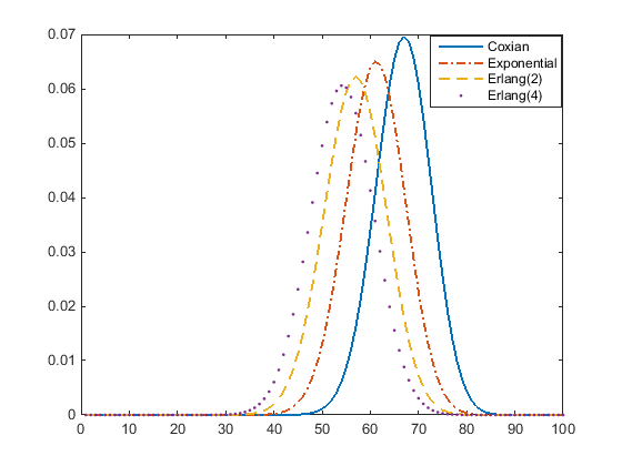
In the following two figures we vary the buffer capacity ; the process we considered was the MAFP with OFF-times having a Coxian distribution. The parameters of the distribution are the same as above for the MAFP.


In the figure below we consider the M/G/1 queue (left figure) and we vary the arrival rate in order to study the occupation time for different values of the occupation rate . The service time has an Erlang distribution with two phases and . In the second figure we study the convergence of the distribution function of the occupation time for the case all the positive rates are set equal and take the limit as , see also Section 3.2. In this case we consider a MAFP with Coxian ON-times with parameters as above.


Acknowledgements
We would like to thank the associate editor for his inspiring comments and the anonymous referee who analysed the paper with great care. Their suggestions helped us improve the paper significantly.
The research of N. Starreveld and M. Mandjes is partly funded by the NWO Gravitation project Networks, grant number 024.002.003.
References
- [1] J. Abate and W. Whitt (2006). A unified framework for numerically inverting Laplace transforms. INFORMS Journal on Computing, Vol. 18, pp. 408-421.
- [2] S. Asmussen (2003). Applied Probability and Queues, 2nd edition. Springer, New York.
- [3] S. Asmussen (2014). Lévy processes, phase-type distributions and martingales. Stochastic Models, Vol. 30, pp. 443-468.
- [4] S. Asmussen and O. Kella (2000). A Multi-dimensional Martingale for Markov Additive Processes and its Applications. Advances in Applied Probability, Vol. 32, No. 2, pp. 376-393.
- [5] O. Baron and J. Milner (2009). Staffing to maximize profit for call centers with alternate service-level agreements. Operations Research, Vol. 57, pp. 685-700.
- [6] N. Bean, M. O’Reilly and P. Taylor (2009). Hitting probabilities and hitting times for stochastic fluid flows: The bounded model. Probability in the Engineering and Informational Sciences, 23(1), 121-147.
- [7] L. Breuer (2012). Occupation Times for Markov-Modulated Brownian Motion. Journal of Applied Probability, 49(2), pp. 549–565.
- [8] J. Cohen and M. Rubinovitch (1977). On level crossings and cycles in dam processes. Mathematics of Operations Research, Vol. 2, pp. 297-310.
- [9] K. Debicki and M. Mandjes (2015). Queues and Lévy Fluctuation Theory. Springer, New York.
- [10] J. Ivanovs, O. Boxma and M. Mandjes (2010). Singularities of the matrix exponent of a Markov additive process with one-sided jumps. Stochastic Processes and their Applications, Vol. 120, Issue 9, pp. 1776–1794.
- [11] O. Kella (2006). Reflecting thoughts. Statistics and Probability Letters, 76(16), pp. 1808-1811.
- [12] L. Kruk, J. Lehoczky, K. Ramanan and S. Shreve (2007). An explicit formula for the Skorokhod map on . The Annals of Probability, Vol. 35, No. 5, 1740-1768.
- [13] A. Kyprianou, J. Pardo and J. Pérez (2014). Occupation times of refracted Lévy processes. Journal of Theoretical Probability, Vol. 27, pp. 1292-1315.
- [14] D. Landriault, J. Renaud and X. Zhou (2011). Occupation times of spectrally negative Lévy processes with applications. Stochastic Processes and their Applications, Vol. 121, pp. 2629-2641.
- [15] R. Loeffen, J. Renaud and X. Zhou (2014). Occupation times of intervals until passage times for spectrally negative Lévy processes. Stochastic Processes and their Applications, Vol. 124, pp. 1408-1435.
- [16] A. Roubos, R. Bekker and S. Bhulai (2015). Occupation times for multi-server queues. Submitted.
- [17] A. Roubos, G.M. Koole and R. Stolletz (2012). Service-level variability of inbound call centers. Manufacturing & Service Operations Management, Vol. 14, pp. 402-413.
- [18] N. J. Starreveld, R. Bekker and M. Mandjes (2016). Occupation times for regenerative processes with Lévy applications. Submitted. arXiv:1602.05131.
- [19] L. Takács (1957). On certain sojourn time problems in the theory of stochastic processes. Acta Mathematica Academiae Scientiarum Hungarica, Vol. 8, pp. 169-191.
- [20] S. Zacks (2012). Distribution of the total time in a mode of an alternating renewal process with applications. Sequential Analysis, Vol. 31, pp. 397-408.