Modeling and Identification of Worst-Case Cascading Failures in Power Systems

The cascading model describes the evolution of branch admittance as a result of overloading on transmission lines and the ensuing branch outage. To characterize the connection state of transmission line, we introduce the state function of the transmission line that connects Bus $i$ and Bus $j$ as follows

$$g(P_{ij},c_{ij})=\left\{\begin{array}[]{ll}0,&\hbox{$|P_{ij}|\geq\sqrt{c_{ij}^{2}+\frac{\pi}{2\sigma}}$;}\\ 1,&\hbox{$|P_{ij}|\leq\sqrt{c_{ij}^{2}-\frac{\pi}{2\sigma}}$;}\\ \frac{1-\sin\sigma(P_{ij}^{2}-c_{ij}^{2})}{2},&\hbox{otherwise.}\end{array}\right.$$

(1)

where $i$,$j\in I_{n_{b}}=\{1,2,...,n_{b}\}$, $i\neq j$ and $n_{b}$ is the total number of buses in the power system. $\sigma$ is a tunable positive parameter. $P_{ij}$ refers to the transmitted power on the transmission line that links Bus $i$ and Bus $j$, and $c_{ij}$ denotes its power threshold. The state function $g(P_{ij},c_{ij})$ is differentiable with respect to $P_{ij}$, and it more closely resembles the step function as $\sigma$ increases (see Fig. 2). The transmission line is in good condition when $g(P_{ij},c_{ij})=1$, while $g(P_{ij},c_{ij})=0$ implies that the transmission line has been severed by the circuit breaker.

The cascading model of power systems at the $k$-th step can be presented as

$$Y_{p}^{k+1}=G(P_{ij}^{k},c_{ij})\cdot Y_{p}^{k}+E_{i_{k}}u_{k},\quad k=0,1,2,...m-1$$

(2)

where $Y_{p}^{k}=(y^{k}_{p,1},y^{k}_{p,2},...,y^{k}_{p,n})^{T}$ is the admittance vector for the $n$ transmission lines or branches at the $k$-th step, and $u_{k}=(u_{k,1},u_{k,2},...,u_{k,n})^{T}$ denotes the control input on transmission lines. $m$ is the total number of cascading steps in power networks. $G(P_{ij}^{k},c_{ij})$ and $E_{i_{k}}$ are the diagonal matrixes defined as

$$G(P_{ij}^{k},c_{ij})=\left(\begin{array}[]{cccc}g(P^{k}_{i_{1}j_{1}},c_{i_{1}j_{1}})&0&.&0\\ 0&g(P^{k}_{i_{2}j_{2}},c_{i_{2}j_{2}})&.&0\\ .&.&.&.\\ 0&0&.&g(P^{k}_{i_{n}j_{n}},c_{i_{n}j_{n}})\\ \end{array}\right)$$

and

$$E_{i_{k}}=diag\left(e^{T}_{i_{k}}\right)=diag(\underbrace{0,..,0,1}_{i_{k}},0,...,0)\in R^{n\times n}.$$

Here $E_{i_{k}}$ is used to select the $i_{k}$-th branch to add the control input on. The intuitive interpretation of Cascading Model (2) is that the admittance of transmission line becomes zero and remains unchanged after the branch outage and that the control input is added on the selected transmission line to directly change its admittance at the initial step.

In this work, we focus on the state evolution of transmission lines or mains in power systems and thus compute the DC power flow to deal with the overloading problem. Specifically, the DC power flow equation is given by

$$P_{i}=\sum_{j=1}^{n_{b}}B_{ij}\theta_{ij}=\sum_{j=1}^{n_{b}}B_{ij}(\theta_{i}-\theta_{j})$$

(3)

where $P_{i}$ and $\theta_{i}$ refer to the injection power and voltage phase angle of Bus $i$, respectively. $B_{ij}$ represents the mutual susceptance between Bus $i$ and Bus $j$, where $i,j\in I_{n_{b}}$. Equation (3) can be rewritten in matrix form [14]

$$P=B\theta$$

where

$$P=\left(\begin{array}[]{c}P_{1}\\ P_{2}\\ .\\ P_{n_{b}}\\ \end{array}\right),\quad B=\left(\begin{array}[]{cccc}\sum_{i=2}^{n_{b}}B_{1i}&-B_{12}&.&B_{1n_{b}}\\ -B_{21}&\sum_{i=1,i\neq 2}^{n_{b}}B_{2i}&.&B_{2n_{b}}\\ .&.&.&.\\ -B_{n_{b}1}&-B_{n_{b}2}&.&\sum_{i=1}^{n_{b}-1}B_{n_{b}i}\\ \end{array}\right),\quad\theta=\left(\begin{array}[]{c}\theta_{1}\\ \theta_{2}\\ .\\ \theta_{n_{b}}\\ \end{array}\right)$$

Actually, $B$ is the nodal admittance matrix of power networks while using the DC power flow. The nodal admittance matrix $Y^{k}_{b}$ at the $k$-th time step can be obtained as

$$Y^{k}_{b}=A^{T}diag(Y^{k}_{p})A$$

where $A$ denotes the branch-bus incidence matrix [15]. Therefore, the matrix $B$ at the $k$-th time step of cascading failure can be calculated as

$$B^{k}=Y^{k}_{b}=A^{T}diag(Y^{k}_{p})A,\quad Y^{k}_{p}=(y^{k}_{p,1},y^{k}_{p,2},...,y^{k}_{p,n})^{T},\quad y^{k}_{p,i}=-\frac{1}{Im(z^{k}_{p,i})},\quad i\in I_{n}=\{1,2,...,n\}$$

where $z^{k}_{p,i}$ denotes the impedance of the $i$-th branch at the $k$-th time step. Then the DC power flow equation at the $k$-th time step is given by

$$P^{k}=B^{k}\theta^{k}=Y_{b}^{k}\theta^{k}$$

(4)

where $P^{k}=(P^{k}_{1},P^{k}_{2},...,P^{k}_{n_{b}})^{T}$ and $\theta^{k}=(\theta^{k}_{1},\theta^{k}_{2},...,\theta^{k}_{n_{b}})^{T}$. During the cascading blackout, the power network may be divided into several subnetworks ($i.e.$, islands), which can be identified by analyzing the nodal admittance matrix $Y^{k}_{b}$. Suppose $Y^{k}_{b}$ is composed of $q$ isolated components or subnetworks denoted by $\mathrm{S}_{i},i\in I_{q}=\{1,2,...,q\}$ and each subnetwork $\mathrm{S}_{i}$ includes $k_{i}$ buses, $i.e.$, $\mathrm{S}_{i}=\{i_{1},i_{2},...,i_{k_{i}}\}$, where $i_{1}$, $i_{2}$,…, $i_{k_{i}}$ denote the bus identity (ID) numbers and $\sum_{i=1}^{q}k_{i}=n_{b}$. Notice that Bus $i_{1}$ in Subnetwork $\mathrm{S}_{i}$ is designated as the reference bus, which is normally a generator bus in practice. The nodal admittance matrix of the $i$-th subnetwork can be computed as

$$Y^{k}_{b,i}=\left(\begin{array}[]{c}e_{i_{1}}^{T}\\ e_{i_{2}}^{T}\\ .\\ e_{i_{k_{i}}}^{T}\\ \end{array}\right)Y^{k}_{b}\left(e_{i_{1}},e_{i_{2}},...,e_{i_{k_{i}}}\right),\quad i\in I_{q}$$

For simplicity, we introduce two operators $*$ and $-1^{*}$ to facilitate the analytical expression and theoretical analysis of solving the DC power flow equation.

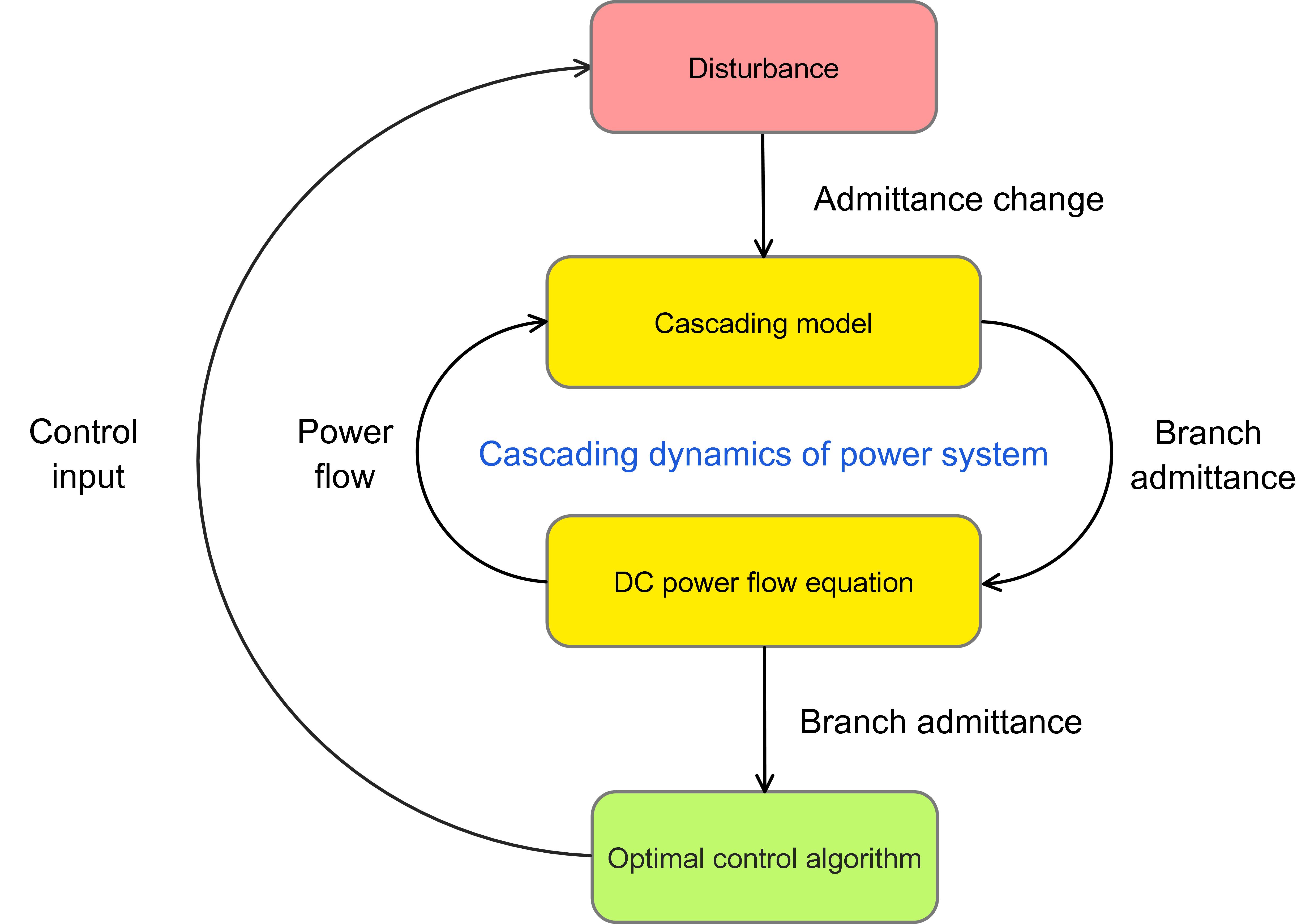
The cascading dynamics of power system is composed of the cascading model defined by Equation (2) and DC power flow equation described by Equation (4), and these two components are coupled with each other, which characterizes the cascading blackout of power grids after suffering from disruptive disturbances. The optimal control algorithm allows us to obtain the disruptive disturbances by treating the disturbances as the control inputs of the optimal control system (see Fig. 3). Specifically, the cascading model describes the outage of overloading branches and updates the admittance on transmission lines with the latest power flow, which is provided by the DC power flow equation. Meanwhile, the DC power flow equation is solved with the up-to-date admittance of branches from the cascading model. The above two processes occur iteratively in describing the evolution of admittance and transmission power on transmission lines. Moreover, the cascading dynamics of power system exactly functions as the state equation of optimal control system. In this way, the optimal control algorithm allows us to gain the control input or disruptive disturbance that triggers the chain reaction of the proposed cascading model.

The identification of disruptive disturbances in power systems can be formulated as the following optimal control problem.

$$\min_{u_{k}}J(Y_{p}^{m},u_{k})$$

(5)

with the cost function

$$J(Y_{p}^{m},u_{k})=\mathrm{T}(Y_{p}^{m})+\epsilon\sum_{k=0}^{m-1}\frac{\|u_{k}\|^{2}}{\max\{0,\iota-k\}}$$

(6)

where $\mathbf{1}_{n}=(1,1,...,1)^{T}\in R^{n}$ and $\epsilon$ is a positive weight. $\|\cdot\|$ represents the 2-norm. As mentioned before, the state equation of the optimal control system consists of Equations (2) and (4). The above cost function includes two terms. Specifically, the first term $\mathrm{T}(Y_{p}^{m})$ is differentiable with respect to $Y_{p}^{m}$, and it quantifies the power state or connectivity of power networks at the final step of cascading blackout, and the second term characterizes the control energy at the first $\iota$ time steps with the constraint $1\leq\iota\leq(m-1)$. In practice, $\mathrm{T}(Y_{p}^{m})$ is designed according to the specific concerns about the worst-case scenario in power systems. In particular, the parameter $\epsilon$ is set small enough so that the first term dominates in the cost function. The objective is to minimize $\mathrm{T}(Y_{p}^{m})$ by adding the appropriate control input $u_{k}$ on the branches of power systems at the given time step.

The parameter settings of IEEE 9 Bus System (see Fig. 4) are presented in Table 2 and Table 3 [19]. It is worth noting that R represents the reference bus (slack bus). G refers to the generator bus and L stands for the load bus in Table 3. Per unit values are adopted with the base value $100$MVA. Other parameters for the dynamic model of power system are given as $\sigma=5\times 10^{4}$, $\iota=1$, $\epsilon=10^{-4}$, $i_{\max}=10$, $J_{\max}=10^{6}$ and $m=9$. The solver “fsolve” in Matlab is employed to solve the system of algebraic equations (11).

Figure 5 shows the computed disturbance and corresponding cost for each branch by the ISA in Table 1. It is observed that the disturbance on Branch 2 results in the least cost, which indicates the most outage branches in the final step. In particular, Fig. 6 presents the time evolution while applying the ISA to search for the desired disturbance or optimal control input on Branch 2 in 10 rounds. After 7 rounds, the cost function is lowered greatly to the bottom and keeps invariant afterwards. Correspondingly, the computed control input converges to $10.87$, which exactly severs Branch 2.

Branch $2$ is selected to add the disruptive disturbance that initiates the chain reaction of cascading blackout. In Fig. 7, red balls denote the generator buses, and green ones refer to the load buses. Bus identity (ID) numbers and branch ID numbers are marked as well. The arrows represent the power flow on each branch. A branch is severed once its transmission power exceeds the given threshold. The arrow disappears if there is no power transmission on the branch. The power system is running in the normal state at Step 1. Then the disruptive disturbance computed by the ISA (susceptance decrement 10.87) is added to sever Branch 2 at Step 2. Then Branch 1, Branch 4 and Branch 5 break off simultaneously at Step 3. Subsequently, Branch 3, Branch 6, Branch 7 and Branch 9 are removed from the power system at Step 4. As a result, the power network is divided into 8 islands without any power consumption. In particular, there is no power transmission on Branch 8 since Bus 6 and Bus 9 are both load buses.

References

- [1] Final Report on the August 14, 2003 Blackout in the United States and Canada. Electricity Markets and Policy Group Technical report, US-Canada Power System Outage Task Force, 2004.
- [2] Final Report System Disturbance on 4 November 2006. Technical Report, Union for the Co-ordination of Transmission of Electricity, 2007.
- [3] Hines, Paul DH, and Pooya Rezaei. Cascading Failures in Power Systems. Smart Grid Handbook, 2016.
- [4] Dobson, I., Carreras, B.A., Lynch, V.E., and Newman, D.E. Complex systems analysis of series of blackouts: cascading failure, critical points, and self-organization. Chaos: An Interdisciplinary Journal of Nonlinear Science 17, 026103, 2007.
- [5] Vaiman, M., Bell, K., Chen, Y., et al. Risk assessment of cascading outages: methodologies and challenges. IEEE Transactions on Power Systems 27 (2), 631641, 2012.
- [6] Hines, P., Cotilla-Sanchez, E., and Blumsack, S. Do topological models provide good information about vulnerability in electric power networks ? Chaos: An Interdisciplinary Journal of Nonlinear Science 20 (3), 033122, 2010.
- [7] Yu, Y., Xiao, G., Zhou, J., Wang, Y., Wang, Z., Kurths, J., Schellnhuber, H. J., System crash as dynamics of complex networks. Proceedings of the National Academy of Sciences, 201612094, 2016.
- [8] Cate, E.G., Hemmaplardh, K., Manke, J.W., and Gelopulos, D.P. Time frame notion and time response of the models in transient, mid-term and long-term stability programs. IEEE Transactions on Power Apparatus and Systems PAS-103 (1), 143151, 1984.
- [9] Roytelman, I. and Shahidehpour, S.M. A comprehensive long term dynamic simulation for power system recovery. IEEE Transactions on Power Systems 9 (3), 14271433, 1994.
- [10] Song, J., Cotilla-Sanchez, E., Ghanavati, G., Hines, P. D. Dynamic modeling of cascading failure in power systems. IEEE Transactions on Power Systems, 31(3): 2085-2095, 2016.
- [11] Kim, Taedong, Stephen J. Wright, Daniel Bienstock, and Sean Harnett, Analyzing vulnerability of power systems with continuous optimization formulations, IEEE Transactions on Network Science and Engineering 3(3): 132-146, 2016.
- [12] Tarsi, David. Simultaneous Solution of line-out and open-end line-to-ground short circuits. IEEE Transactions on Power Apparatus and Systems, 6(PAS-89): 1220-1225, 1970.
- [13] Perez LG, Flechsig AJ, Venkatasubramanian VA, Modeling the protective system for power system dynamic analysis, IEEE Transactions on Power Systems, 9(4): 1963-1973, 1994.
- [14] Stott, B., Jardim, J. and Alsaç, O., DC power flow revisited. IEEE Transactions on Power Systems, 24(3): 1290-1300, 2009.
- [15] Stagg, Glenn W., and Ahmed H. El-Abiad. Computer Methods in Power System Analysis. McGraw-Hill, 1968.
- [16] Godsil, Chris, and Gordon F. Royle. Algebraic graph theory. Vol. 207. Springer Science & Business Media, 2013.
- [17] Frank L. Lewis and Vassilis L. Syrmos. Optimal Control, 2nd Edition. Wiley-Interscience, 2nd edition, October 1995.
- [18] Yeh, James. Real Analysis: Theory of Measure and Integration. World Scientific, 2006.
- [19] R. D. Zimmerman, C. E. Murillo-Sánchez, and R. J. Thomas, Matpower: Steady-state operations, planning and analysis tools for power systems research and education, IEEE Transactions on Power Systems, vol. 26, no. 1, pp. 12-19, Feb. 2011.
- [20] Hong, Y., Zhai, C., Dynamic coordination and distributed control design of multi-agent systems, Control Theory & Applications, 10, 028, 2011.
- [21] Zhai, C., Hong, Y., Decentralized sweep coverage algorithm for uncertain region of multi-agent systems, Proceedings of American Control Conference, Montréal, Canada, pp. 4522-4527, 2012.