Budgeted Batch Bayesian Optimization With Unknown Batch Sizes

Gaussian processes (GP) (?) extends a multivariate Gaussian distribution to infinite dimensionality. Formally, Gaussian process generates data located throughout some domains such that any finite subset of the range follows a multivariate Gaussian distribution. Given $N$ observations $\boldsymbol{Y}=\left\{y_{1},y_{2},...y_{N}\right\}$ which can always be imagined as a single point sampled from some multivariate Gaussian distributions.

The mean of GP is assumed to be zero everywhere. What relates one observation to another in such cases is just the covariance function, $k\left(x,x^{\prime}\right)$. From the assumption of GP, we have $\boldsymbol{y}\sim\mathcal{N}\left(0,\boldsymbol{K}\right)$ where the covariance matrix is defined as follows:

A popular choice for the covariance function $k$ is the squared exponential function: $k\left(x,x^{\prime}\right)=\sigma_{f}^{2}\exp\left[\frac{-\left(x-x^{\prime}\right)^{2}}{2l^{2}}\right]$ where $\sigma_{f}^{2}$ defines the maximum allowable covariance. It $x\thickapprox x^{\prime}$, then $k\left(x,x^{\prime}\right)$ approaches this maximum of $\sigma_{f}^{2}$, indicating that $f(x)$ is perfectly correlated with $f(x^{\prime})$. If $x$ is far from $x^{\prime}$, we have instead $k\left(x,x^{\prime}\right)\thickapprox 0$. The length parameter $l$ will control this separation when $x$ is not closed to $x^{\prime}$.

For prediction on a new data point $y_{*}$, we can update the covariance matrix with $k_{**}=k\left(x_{*},x_{*}\right)$ and $\boldsymbol{k}_{*}=\begin{array}[]{cccc}k\left(x_{*},x_{1}\right)&k\left(x_{*},x_{2}\right)&\cdots&k\left(x_{*},x_{N}\right)\end{array}$ . Hence, we can write

The conditional probability is followed Gaussian distribution as $p\left(y_{*}\mid\boldsymbol{y}\right)\sim\mathcal{N}\left(\mu\left(\boldsymbol{x}_{*}\right),\sigma^{2}\left(\boldsymbol{x}_{*}\right)\right)$ (?, ?) where its mean and variance are given by

GPs provide a full probabilistic model of the data, and allow us to compute not only the model’s prediction at input points but also to quantify the uncertainty in the predictions. Therefore, GP is flexible as a nonparametric prior for Bayesian optimization.

We assume that $f$ is a black-box function, that is, its form is unknown and further it is expensive to evaluate. Perturbed evaluations of the type $y_{i}=f\left(\boldsymbol{x}_{i}\right)+\epsilon_{i}$, where $\epsilon_{i}\sim\mathcal{N}\left(0,\sigma^{2}\right)$, are available. Example of the Branin function is in Fig. 1. Bayesian optimization makes a series of evaluations $\boldsymbol{x}_{1},...,\boldsymbol{x}_{T}$ of $f$ such that the maximum of $f$ is found in the fewest iterations (?, ?, ?, ?). Formally, let $f:\mathcal{X}\rightarrow\mathcal{R}$ be a well behaved function defined on a compact subset $\mathcal{X}\subseteq\mathcal{R}^{D}$. Our goal is solving the global optimization problem

Bayesian optimization reasons about $f$ by building a Gaussian process through evaluations (?). This flexible distribution allows us to associate a normally distributed random variable at every point in the continuous input space.

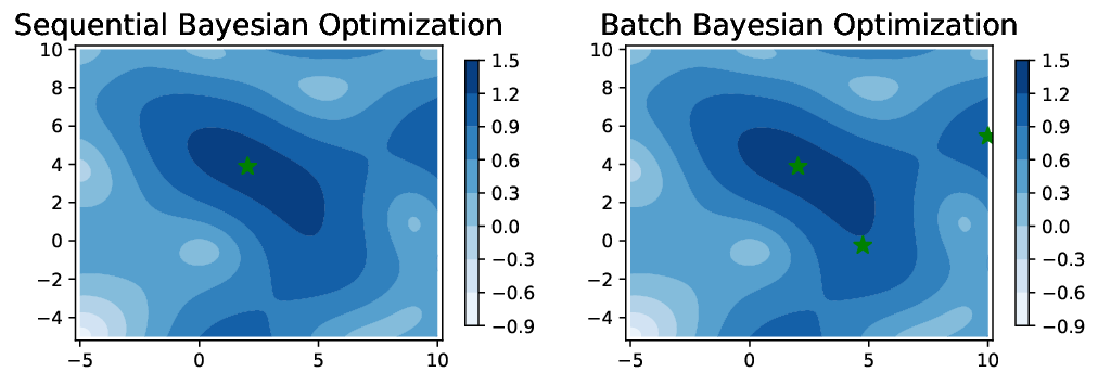
Bayesian optimization is conventionally posed as a sequential problem where each experiment is completed before taking a new one. In practice it may be advantageous to run multiple function evaluations in parallel. Therefore, we consider evaluating $f$ using a batch of points. An example of batch Bayesian optimization versus sequential Bayesian optimization is illustrated in Fig. 2. As discussed earlier, such scenarios appear, for instance, in the optimization of computer models where several machines (or cores) are available to run experiments in parallel, or in wet-lab experiments when the time of testing one experimental design is the same as testing a batch. Formally, we maximize the acquisition function by finding a collection of points as

where $n_{t}$ is the batch size at iteration $t$. Existing approaches often fix the batch size $n_{t}$ to a constant value for all iterations.

Since the optimization in Eq. 2 is intractable, batch BO techniques avoid this computational burden by resorting to different strategies. The first BO parallelization was used in the context of the learning Bayesian networks (?), to the best of our knowledge. Then batch BO simulation matching (?) aims to select a batch of size $q$, which includes points ‘close to’ the best point.

Developing from the expected improvement acquisition function (EI), the multi-point expected improvement (q-EI)(?) treats the acquisition function as the conditional expectation of the improvement obtained by $q$ points. Constant Liar (CL) is a heuristic q-EI algorithm (?), which uses a greedy approach to iteratively construct a batch of $q$ points. At each iteration, the heuristic uses the sequential algorithm to find a point that maximizes the expected improvement as follows: first, the maximum of the acquisition is found and to move to the next maximum by suppressing this point. This is done by inserting the outcome at this point as a constant value. The GP posterior is updated through the “fake” outcome which then is used to compute the acquisition function. This process is repeated until the batch is filled. Further parallel extension for q-EI are proposed in (?, ?).

Another direction (?, ?) in batch Bayesian optimization exploits an interesting fact about GPs: the predictive variance of GPs depends only on the feature $\boldsymbol{x}$, but not the outcome values $\boldsymbol{y}$. The GP-BUCB algorithm (?) and GP-UCB-PE (?) extend the sequential UCB to a batch setting by first selecting the next point, updating the predictive variance which in turn alters the acquisition function, and then selecting the next point. This is repeated till the batch is filled. In particular, the GP-UCB-PE (?) chooses the first point of the batch via the UCB score and then defines a “relevance region” and selects the remaining points from this region greedily to maximize the information gain, to focus on pure exploration (PE).

Batch BO can also be developed using information-based policies (?). PES aim to select the point which maximizes the information gain of the model. This is solved by expressing the expected reduction in the differential entropy of the predicted distribution. Parallel Predictive Entropy Search (PPES) (?) extends the Predictive Entropy Search (PES) algorithm of (?) to a batch setting.

More recently, Local Penalization (LP) (?) presents a heuristic approach for batch BO by iteratively penalizing the current peak in the acquisition function to find the next peak. LP depends on the estimation of Lipschitz constant to flexibly penalize the peaks. However, in general scenarios, the Lipschitz constant $L$ is unknown. For ease of computation, (?) estimates the Lipschitz constant of the GP predictive mean instead of the actual acquisition function. Furthermore, the use of a unique value of $L$ assumes that the function is Lipschitz homoscedastic. Gonzalez et al (?) has demonstrated that LP outperforms a wide range of baselines in batch Bayesian optimization. We thus consider LP as the most competitive baseline in batch BO.

Although the batch algorithms can speedup the selection of experiments, there are two main drawbacks. First, most of the proposed batch BO (?, ?, ?, ?, ?, ?) involve a greedy algorithm, which chooses individual points until the batch is filled. This is often detrimental as the requirement to fill a batch enforces the selection of not only the true maxima but also noisy peaks. Second, most approaches use a predefined and fixed batch size $q$ for all iterations. Fixed batch size may be inefficient because the number of peaks in the acquisition function is unknown and constantly changing when the GP posterior is updated. For example, if a function has two real maxima, a batch size of more than two will force the selection of noisy points. Therefore, time and resources are wasted for evaluating these noisy points that contravening the goal of BO is to save the number of evaluations. In contrast, if we under-specify the number of peaks, we could miss important points that may be the optimal solution of $f$. Hence, it is necessary to identify the appropriate, if not exact, number of peaks for evaluation while preserving the ability of finding the optimal value of $f$.

We consider the batch Bayesian optimization. As a Bayesian optimization task, our ultimate goal is solving the global optimization problem of finding $\boldsymbol{x}^{*}=\underset{\boldsymbol{x}\in\mathcal{X}}{\text{argmax}\thinspace f\left(\boldsymbol{x}\right)}$ by making a series of batch evaluations $\boldsymbol{X}_{t},\boldsymbol{X}_{2}...\boldsymbol{X}_{T}$ where $\boldsymbol{X}_{t}=\left[\boldsymbol{x}_{t1},\boldsymbol{x}_{t2},...,\boldsymbol{x}_{tn_{t}}\right]$ such that the maximum of $f$ is found (?, ?) where $n_{t}$ is the batch size.

The acquisition function $\alpha$ is often multi-modal with the unknown number of peaks. It is intuitive to assume that the acquisition function can be approximated by a mixture of Gaussians (cf. Fig. 3) wherein the peaks in the acquisition function are equivalent to the mean locations of the underlying Gaussians. Because the number of peaks are unknown, we borrow the elegance of Bayesian nonparametrics (?) to identify the unknown number of Gaussian components. We use the infinite Gaussian mixture model (IGMM) (?) which induces the Dirichlet Process prior over possibly infinite number of Gaussian components. In IGMM, each Gaussian component representing a peak $k$ is parameterized by the mean $\mu_{k}$ and the covariance $\Sigma_{k}$. It is interesting that the estimated mean $\mu_{k}$ is the location of the peaks while the estimated covariance $\Sigma_{k}$ will capture the shape of the peaks in the acquisition function. In contrast, previous work (?) relies on an unique Lipschitz constant to represent the shape of the peak that is not reasonable for the heteroscedastic setting when the peaks have different shapes. Formally, the probability density function of the IGMM is defined as follows $\sum_{k=1}^{\infty}\pi_{k}\times\mathcal{N}\left(s\mid\mu_{k},\Sigma_{k}\right)$ where $s$ is an observation, $\pi_{k}$ is the mixing proportion in IGMM and $\mathcal{N}\left(s\mid\mu_{k},\Sigma_{k}\right)$ is the Gaussian density function of the component $k$.

Our primary goal in utilizing IGMM is to approximately find the mean $\mu_{k}$(s) of Gaussian distributions as the unknown peaks from the acquisition function. However, directly estimating IGMM from acquisition function is intractable. Therefore, we use the intermediate step to draw samples under the acquisition function and then fit the IGMM to learn the mean locations as the batch of points to evaluate.

We now present the sampling technique to draw samples under the acquisition function for fitting to the IGMM. We note that the sampling process, by its nature, generates more samples from high probability regions. This implies that most of the samples come from the peaks. Thus, even with small number of samples, the sampling process approximates the peaks and is then efficient. There are many existing sampling methods to draw samples from the probability distributions, for example, Metropolis-Hastings (?). However, to sample under the $D$-dimensional acquisition function which is not strictly probability distribution, we utilize the accept-reject sampling (?) where we keep samples in the region under the density function and ignore samples if they are outside the curve.

In particular, we select to use the slice sampling (?) because it is easily implemented for univariate distributions, and can be used to sample from a multivariate distribution by updating each variable in turn. Suppose we wish to sample from a distribution for a variable, $x$, taking values in some subset of $\mathcal{R}^{D}$, whose density is proportional to some functions $g(x)$. We can do this by sampling uniformly from the $(D+1)$-dimensional region that lies under the plot of $g(x)$. This idea can be formalized by introducing an auxiliary real variable, $u$, and defining a joint distribution over $x$ and $u$ that is uniform over the region $R=\left\{(x,u):0<u<g(x)\right\}$ below the curve or surface defined by $g(x)$. The joint density for $(x,u)$ is

where $Z=\int g\left(x\right)dx$. The marginal density for $x$ is then $p\left(x\right)=\int_{0}^{g(x)}\frac{1}{Z}du=\frac{g\left(x\right)}{Z}$. To sample for $x$, we can sample jointly for $(x,u)$, and then ignore $u$.

We extend the standard slice sampler to the generalized slice sampler that draws samples from $D$-dimensional acquisition function $\alpha$ which is not a proper distribution and can be negative. To draw $u$ uniformly over the region $R$ below curve of the acquisition function, we get the $\alpha_{\textrm{min}}=\min_{x\in\mathcal{X}}\alpha\left(x\right)$ obtained by one of the non-convex optimization toolbox (e.g., DIRECT (?)). Therefore, we can define the joint density

where $Z=\int\alpha\left(x\right)dx$. The marginal density for $x$ is then $p\left(x\right)=\int_{\alpha_{\textrm{min}}}^{\alpha(x)}\frac{1}{Z}du=\frac{\alpha\left(x\right)-\alpha_{\textrm{min}}}{Z}$. To sample for $x$, we can sample jointly for $(x,u)$, and then ignore $u$ following the Algorithm 3.1 and Fig. 4 where $\textrm{uniform}\left(\boldsymbol{x}_{\textrm{min}},\boldsymbol{x}_{\textrm{max}}\right)$ denotes for drawing randomly from the uniform distribution within the bound of $\left[\boldsymbol{x}_{\textrm{min}},\boldsymbol{x}_{\textrm{max}}\right]$, which is predefined.

Slice sampling approach (?) also brings a challenge for high-dimensional data that it is hard to find accepted area $R$ such that $g\left(R\right)>u$. There are two main reasons. First, the set of accepted samples could be very small with respect to the hyper-rectangle $R$. Second, $R$ usually lies in a high-dimensional space, implying the curse of dimensionality. Therefore, it is a big drawback of slice sampling to deal with high dimensions (?, ?).

To overcome the problem in high-dimensional functions, we utilize the generalized slice sampler in batch setting where a bunch of samples are drawn i.i.d at different places. Since our goal is to draw a collection of i.i.d. samples $x_{1,2,...N}$ from the acquisition function $\alpha$ (to later estimate the IGMM). We define a collection of joint density distribution $p\left(x_{1},u_{1}\right),...p\left(x_{M},u\right)$ and perform the generalized slice sampling for each joint distribution independently. In the experiment, we set $M$ as $200$. In Sec 4.5, we further study the computational efficiency of the batch generalized slice sampling (BGSS) for drawing samples from high dimensional acquisition functions (e.g., $D=50$).

IGMM is the nonparametric mixture model where the prior distribution over the mixing proportion is a Dirichlet process (?). There are few existing approaches to learn a IGMM, such as collapsed Gibbs sampler (?) and variational inference (?). In this paper, we follow (?) to derive the variational inference for IGMM (?) since the variational approach is generally faster than the Gibbs sampler. After fitting the IGMM using variational inference, we obtain the mean locations $\mu_{1....K}$ as the selected points for evaluations in the batch BO setting. We note that $K$ is unknown and identified automatically in this Bayesian nonparametric setting.

Using the collection of samples $\left(\boldsymbol{s}_{i}\right)_{i=1}^{N}$ drawn from our batch generalized slice sampler, we consider the IGMM generated as follows. We first draw a mixing proportion from the stick-breaking process given the concentration parameter $\gamma$ as $\pi_{k}\sim v_{k}\prod_{l=1}^{k-1}\left(1-v_{l}\right)$ where $v_{k}\sim\text{Beta}\left(1,\gamma\right)$. Next, for each component $k$ in the model, we sample the mean $\mu_{k}\sim\mathcal{N}\left(\mu_{0},\mathbf{I}\right)$ and the covariance matrix $\Sigma_{k}\sim\text{Wish}\left(\tau_{k},\mathbf{I}\right)$. Finally, we generate the assignment $z_{i}\sim\textrm{Stick}\left(\pi\right)$ and the observation $\boldsymbol{s}_{i}\sim\mathcal{N}\left(\mu_{z_{i},}\Sigma_{z_{i}}\right)$.

For posterior inference using variational inference, we first write the bound on the likelihood of the data as follows:

To define the variational distribution $q$ in the Eq. (3), we need to construct a distribution on an infinite set of random variables $v_{k},$$\mu_{k}$ and $\Sigma_{k}$. For this approach be tractable, we truncate the variational distribution at some value $K$ by setting $q(v_{K}=1)=1$ and we can ignore $\mu_{k},\Sigma_{k}$ for $k>K$ (?).

Then, we factorize the variational distribution using mean field assumption as the following $q\left(v,\mu,\Sigma,z\right)=\prod_{k=1}^{K}q\left(v_{k}\mid\eta_{k}\right)q\left(\mu_{k}\mid\lambda_{k}\right)q\left(\Sigma_{k}\mid a_{k},B_{k}\right)\prod_{i=1}^{N}q\left(z_{i}\mid\phi_{i}\right)$. Particularly, the variational distributions for these variables are defined as $q\left(v_{k}\mid\eta_{k}\right)=\text{Beta}\left(\eta_{k1},\eta_{k2}\right),q\left(\mu_{k}\mid\lambda_{k}\right)=\mathcal{N}\left(\lambda_{k},\mathbf{I}\right)$, $q\left(\Sigma_{k}\right)=\textrm{Wishart}(a_{k},B_{k})$ and $q\left(z_{i}\mid\phi_{i}\right)=\text{Mult}\left(\phi_{i}\right)$.

After factorizing the variational distribution using mean field, we maximize the lower bound in Eq. (3). We first take the partial derivative w.r.t. each variational variables. We then equate it to zero and solve the optimization for each variables. Due to the space restriction, we shall refer the detailed inference of the infinite Gaussian mixture model to (?, ?).

Although the technique of variational inference for IGMM and the slice sampling are existed for years, the idea of connecting these things at the right place for batch BO is novel. We summarize the steps for B3O in Algorithm 3.2. At an iteration $t$, we will find a batch including $n_{t}$ points where the number of point $n_{t}$ varies at each iteration.

We note that steps 2,3,7 and 8 are standard in Bayesian optimization techniques. Our proposed method is highlighted in steps 4,5 and 6 to find a batch of points $\boldsymbol{X}_{t}$ from the acquisition function. Particularly, Fig. 3 illustrates and summarizes our steps 4,5 and 6 in 1D and 2D, respectively. We summarize the computation time of steps 4, 5, and 6 in Sec 4.4 and further analyze step 4 by simulation in Sec 4.5 which requires more computation than other steps.

We examine the performance of B3O in finding the optimum of the chosen benchmark functions. We demonstrate that our method can find better optimal values (minimum) for a fixed amount of iterations $T$. We report the best-found-value w.r.t. iterations in Fig. 5. Our method achieves significantly better values than the baselines in 5 over 8 functions. In particular, B3O outperforms all baselines in Forrester $1D$, Alpine2 $5D$, gSobol $5D$, Alpine2 $10D$, gSobol $10D$. In other three cases, B3O still provides relatively good values. The fixed batch approaches (e.g., LP) may suffer the under-specification (the number of specified batch size $n_{t}$ is smaller than the number of real peaks) at some iterations and thus negatively affect the final performance.

As expected, the batch approaches are always better than the sequential approaches using EI and UCB because the number of evaluated points for batch methods is much higher than the sequential. This fact also highlights the advantage of batch BO over the standard (sequential) BO.

The next criteria for comparison is the total number of evaluations, $N=\sum_{t=0}^{T}n_{t}$. The requirement of Bayesian optimization is to keep the number of evaluations to find the optimal value as low as possible, as these evaluations can be costly. For example, it can very expensive to perform a single experiment in material science (to cast an alloy testing), or it takes a few days to train a deep network on a large-scale dataset.

It is not natural to fix the number of evaluations per batch $n_{t}$, since the number of peaks is unknown, and importantly, these peaks will be changed after new evaluations are done. Therefore, we may waste time and resources if we over-evaluate the number of points than we need. In particular, after all the actual peaks are detected, if we set the batch size $n_{t}$ large, we will get the noisy points which are possibly close to the already detected ones due to the effect of penalizing the peaks (?). Hence, these noisy points are not useful for evaluation. In contrast, under-evaluating the number of necessary points also brings detrimental effects of losing the optimal points.

B3O automatically identifies the suitable number of peaks from the acquisition function in each iteration, and thus does not have to resort to a fixed batch sizes. This is efficient without suffering any performance loss. Given a fixed number of iterations $T$, we summarize the total number of evaluations in Fig. 6 - our proposed approach significantly reduces the number of evaluations as compared to the fixed-batch baselines, especially for high dimensional settings, e.g., Alpine2 $10D$ and gSobol $10D$.

We demonstrate that B3O is flexible in identifying the required number of evaluations per batch. We study the number of estimated points in B3O at each iteration. In particular, we record the number of points $n_{t}$ at each iteration, see Fig. 7 for two functions - Dropwave 2D and gSobol 5D. The estimated points per batch in our approach is flexible and determined automatically in this Bayesian nonparametric setting. For some iterations, B3O only recommends one point per batch (see gSobol 5D in Fig. 7). This fact is essential for the homogeneous acquisition function which contains a single peak, whereas the fixed-batch approaches may be wasted to evaluate at some unnecessary points. Moreover, given the fixed batch size for all iterations, other approaches may suffer the effect of over-specification at some iterations and under-specification at other iterations.

Next we compare the computational time at each iteration for the different batch approaches. Specifically, we are interested in the CPU time for finding the batch between different approaches. The sequential methods and the random batch approaches are the cheapest to compute than the other batch approaches. Thus, we do not compare with the sequential and the random batch approaches.

Constant Liar (?) and BUCB (?) take time for re-estimation of the GP when the fake observations are added and noticeably slower when the number of data points $N$ is large. The Local Penalization approach (?) consumes a considerable amount of time to estimate the Lipschitz constant. In addition, LP computes and maintains the penalized cost around the visited points. The cost for penalizing and optimizing will grow for high dimensions and/or large number of observed points.

B3O is generally competitive to LP (?) in terms of computation. We run faster for low dimensional functions (e.g., less than 6 dimensions). However, LP tends to run faster than B3O for 10D functions. We note that in high dimensional functions, the bottle neck in LP is estimating the Lipschitz constant whilst for B3O the batch generalized slice sampling is the bottle neck due to the nature of the sampling algorithm.

We investigate the efficiency of the BGSS presented in Section 3.3 for drawing samples under the acquisition function. We vary the observation dimension $D$ - $5,10,20,40,50$ - and build the acquisition function $\alpha_{UCB}$. Then, we design two BGSS settings of size $100$ and $200$ and compare with the generalized slice sampling which is presented in Fig. 4. We record two important factors including computational time and the number of accepted samples under the curve.

In Fig. 8, we present the simulation results that BGSS significantly outperforms the standard slice sampling in terms of computation (running faster) and efficiency (higher number of accepted points). For example, BGSS of the size $200$ takes $32$ seconds to get $2485$ accepted data points at $D=10$ dimension. These accepted points are lying under the curve and generally surrounding the peak. Therefore, these samples are beneficial to fit the IGMM since we are particularly interested in finding the peaks.

Hyper-parameter settings greatly impact prediction accuracy of machine learning algorithms. The traditional way of performing hyper-parameter tuning has been to perform a grid search. In practice, however, Bayesian optimization has been shown (?, ?, ?) to obtain better results in fewer experiments than required by a full grid search. We employ the batch Bayesian optimization to find the optimal hyper-parameters for support vector regression (SVR), Bayesian nonparametric multi-label classification (BNMC), and multi layer perceptron (MLP).

We consider the alloy hardening process of Aluminum-scandium (?) consisting of two stages: nucleation and precipitation coarsening. We aim to maximize the hardness for Aluminum-scandium alloys by designing the appropriate times and temperatures for the two stages in the process. The traditional approach is to use iterative trial and error, in which we choose some material design (temperature and time) based on intuition, past experience, or theoretical knowledge; and test the material in physical experiments; and then use what we learn from these experiments in choosing the material design to try next. This iterative process is repeated until some combination of success or exhaustion is reached! Since the parameter space grows exponentially, trial and error approach is ill-affordable in terms of both time and cost. Therefor, Bayesian optimization is a necessary choice for this experimental design.

We use B3O for the experimental design problem above and show that our method achieves the highest hardness using the smallest number of experiments (see Table 9a). The heat-treatment profile is shown in Fig. 10 using the best estimated parameters (times and temperatures at two steps) and the best hardness achieved is $88.3$. Given the times and temperatures setting, we evaluate the hardness using the standard kinematic KWN model used by metallurgists (?) .

References

- Azimi, Fern, & Fern Azimi, J., Fern, A., & Fern, X. Z. (2010). Batch bayesian optimization via simulation matching. In Advances in Neural Information Processing Systems, pp. 109–117.
- Azimi, Jalali, & Zhang-fern Azimi, J., Jalali, A., & Zhang-fern, X. (2012). Hybrid batch bayesian optimization. In Proceedings of the 29th International Conference on Machine Learning (ICML-12), pp. 1215–1222.
- Bengio Bengio, Y. (2009). Learning deep architectures for AI. Foundations and Trends in Machine Learning, 2(1), 1–127.
- Bergstra, Bardenet, Bengio, & Kégl Bergstra, J. S., Bardenet, R., Bengio, Y., & Kégl, B. (2011). Algorithms for hyper-parameter optimization. In Advances in Neural Information Processing Systems, pp. 2546–2554.
- Blei, Jordan, et al. Blei, D. M., Jordan, M. I., et al. (2006). Variational inference for dirichlet process mixtures. Bayesian Analysis, 1(1), 121–143.
- Casella, Robert, & Wells Casella, G., Robert, C. P., & Wells, M. T. (2004). Generalized accept-reject sampling schemes. Lecture Notes-Monograph Series, 342–347.
- Contal, Buffoni, Robicquet, & Vayatis Contal, E., Buffoni, D., Robicquet, A., & Vayatis, N. (2013). Parallel gaussian process optimization with upper confidence bound and pure exploration. In Machine Learning and Knowledge Discovery in Databases, pp. 225–240. Springer.
- Cortes & Vapnik Cortes, C., & Vapnik, V. (1995). Support-vector networks. Machine learning, 20(3), 273–297.
- Dai Nguyen, Gupta, Rana, Nguyen, Venkatesh, Deane, & Sanders Dai Nguyen, T., Gupta, S., Rana, S., Nguyen, V., Venkatesh, S., Deane, K. J., & Sanders, P. G. (2016). Cascade bayesian optimization. In Australasian Joint Conference on Artificial Intelligence, pp. 268–280. Springer.
- Desautels, Krause, & Burdick Desautels, T., Krause, A., & Burdick, J. W. (2014). Parallelizing exploration-exploitation tradeoffs in gaussian process bandit optimization. The Journal of Machine Learning Research, 15(1), 3873–3923.
- Drucker, Burges, Kaufman, Smola, Vapnik, et al. Drucker, H., Burges, C. J., Kaufman, L., Smola, A., Vapnik, V., et al. (1997). Support vector regression machines. Advances in neural information processing systems, 9, 155–161.
- Ebden Ebden, M. (2008). Gaussian processes for regression: A quick introduction. The Website of Robotics Research Group in Department on Engineering Science, University of Oxford.
- Ferguson Ferguson, T. S. (1973). A Bayesian analysis of some nonparametric problems. The Annals of Statistics, 1(2), 209–230.
- Frazier & Clark Frazier, P. I., & Clark, S. C. (2012). Parallel global optimization using an improved multi-points expected improvement criterion. In INFORMS Optimization Society Conference, Miami FL, Vol. 26.
- Freitas, Zoghi, & Smola Freitas, N. D., Zoghi, M., & Smola, A. J. (2012). Exponential regret bounds for gaussian process bandits with deterministic observations. In Proceedings of the 29th International Conference on Machine Learning (ICML-12), pp. 1743–1750.
- Ginsbourger, Le Riche, & Carraro Ginsbourger, D., Le Riche, R., & Carraro, L. (2007). A multi-points criterion for deterministic parallel global optimization based on kriging. In NCP07.
- Ginsbourger, Le Riche, & Carraro Ginsbourger, D., Le Riche, R., & Carraro, L. (2008). A multi-points criterion for deterministic parallel global optimization based on gaussian processes..
- Ginsbourger, Le Riche, & Carraro Ginsbourger, D., Le Riche, R., & Carraro, L. (2010). Kriging is well-suited to parallelize optimization. In Computational Intelligence in Expensive Optimization Problems, pp. 131–162. Springer.
- González, Dai, Hennig, & Lawrence González, J., Dai, Z., Hennig, P., & Lawrence, N. D. (2016). Batch bayesian optimization via local penalization. In Proceedings of the 19th International Conference on Artificial Intelligence and Statistics, pp. 648–657.
- Hennig & Schuler Hennig, P., & Schuler, C. J. (2012). Entropy search for information-efficient global optimization. Journal of Machine Learning Research, 13, 1809–1837.
- Hernández-Lobato, Hoffman, & Ghahramani Hernández-Lobato, J. M., Hoffman, M. W., & Ghahramani, Z. (2014). Predictive entropy search for efficient global optimization of black-box functions. In Advances in Neural Information Processing Systems, pp. 918–926.
- Hjort, Holmes, Müller, & Walker Hjort, N., Holmes, C., Müller, P., & Walker, S. (2010). Bayesian nonparametrics. Cambridge University Press.
- Hutter, Hoos, & Leyton-Brown Hutter, F., Hoos, H., & Leyton-Brown, K. (2013). An evaluation of sequential model-based optimization for expensive blackbox functions. In Proceedings of the 15th annual conference companion on Genetic and evolutionary computation, pp. 1209–1216. ACM.
- Jamil & Yang Jamil, M., & Yang, X.-S. (2013). A literature survey of benchmark functions for global optimisation problems. International Journal of Mathematical Modelling and Numerical Optimisation, 4(2), 150–194.
- Jones Jones, D. R. (2001). A taxonomy of global optimization methods based on response surfaces. Journal of global optimization, 21(4), 345–383.
- Jones, Perttunen, & Stuckman Jones, D. R., Perttunen, C. D., & Stuckman, B. E. (1993). Lipschitzian optimization without the lipschitz constant. Journal of Optimization Theory and Applications, 79(1), 157–181.
- Jones, Schonlau, & Welch Jones, D. R., Schonlau, M., & Welch, W. J. (1998). Efficient global optimization of expensive black-box functions. Journal of Global optimization, 13(4), 455–492.
- Kamper Kamper, H. (2013). Gibbs sampling for fitting finite and infinite gaussian mixture models..
- Kampmann & Wagner Kampmann, R., & Wagner, R. (1983). Kinetics of precipitation in metastable binary alloys-theory and applications to cu-1.9 at% ti and ni-14 at% al. In Decomposition of Alloys: The Early Stages, Proceedings of the 2 nd Acta-Scripta Metallurgica Conference, pp. 91–103.
- Khajah, Roads, Lindsey, Liu, & Mozer Khajah, M. M., Roads, B. D., Lindsey, R. V., Liu, Y.-E., & Mozer, M. C. (2016). Designing engaging games using bayesian optimization. In Proceedings of the 2016 CHI Conference on Human Factors in Computing Systems, pp. 5571–5582. ACM.
- Kushner Kushner, H. J. (1964). A new method of locating the maximum point of an arbitrary multipeak curve in the presence of noise. Journal of Basic Engineering, 86(1), 97–106.
- Li, Gupta, Rana, Nguyen, & Venkatesh Li, C., Gupta, S., Rana, S., Nguyen, V., & Venkatesh, S. (2016). High dimensional bayesian optimization with elastic gaussian process. In Workshop on Bayesian Optimization at Neural Information Processing Systems (NIPS).
- Metropolis, Rosenbluth, Rosenbluth, Teller, & Teller Metropolis, N., Rosenbluth, A. W., Rosenbluth, M. N., Teller, A. H., & Teller, E. (1953). Equation of state calculations by fast computing machines. The journal of chemical physics, 21(6), 1087–1092.
- Mockus, Tiesis, & Zilinskas Mockus, J., Tiesis, V., & Zilinskas, A. (1978). The application of bayesian methods for seeking the extremum. Towards global optimization, 2(117-129), 2.
- Neal Neal, R. (2003). Slice sampling. Annals of statistics, 705–741.
- Nguyen, Gupta, Rana, Li, & Venkatesh Nguyen, V., Gupta, S., Rana, S., Li, C., & Venkatesh, S. (2016a). A bayesian nonparametric approach for multi-label classification. In Proceedings of The 8th Asian Conference on Machine Learning, pp. 254–269.
- Nguyen, Gupta, Rana, Li, & Venkatesh Nguyen, V., Gupta, S., Rana, S., Li, C., & Venkatesh, S. (2016b). Think globally, act locally: a local strategy for bayesian optimization. In Workshop on Bayesian Optimization at Neural Information Processing Systems (NIPS).
- Nguyen, Rana, Gupta, Li, & Venkatesh Nguyen, V., Rana, S., Gupta, S. K., Li, C., & Venkatesh, S. (2016c). Budgeted batch bayesian optimization. In Data Mining (ICDM), 2016 IEEE 16th International Conference on, pp. 1107–1112. IEEE.
- Očenášek & Schwarz Očenášek, J., & Schwarz, J. (2000). The parallel bayesian optimization algorithm. In The State of the Art in Computational Intelligence, pp. 61–67. Springer.
- Pietrabissa & Rusconi Pietrabissa, T., & Rusconi, S. (2014). Parallel slice sampling. In The Contribution of Young Researchers to Bayesian Statistics, pp. 81–84. Springer.
- Rasmussen Rasmussen, C. E. (1999). The infinite gaussian mixture model.. In NIPS, Vol. 12, pp. 554–560.
- Rasmussen Rasmussen, C. E. (2006). Gaussian processes for machine learning..
- Ruck, Rogers, Kabrisky, Oxley, & Suter Ruck, D. W., Rogers, S. K., Kabrisky, M., Oxley, M. E., & Suter, B. W. (1990). The multilayer perceptron as an approximation to a bayes optimal discriminant function. Neural Networks, IEEE Transactions on, 1(4), 296–298.
- Shah & Ghahramani Shah, A., & Ghahramani, Z. (2015). Parallel predictive entropy search for batch global optimization of expensive objective functions. In Advances in Neural Information Processing Systems, pp. 3312–3320.
- Shahriari, Swersky, Wang, Adams, & de Freitas Shahriari, B., Swersky, K., Wang, Z., Adams, R. P., & de Freitas, N. (2016). Taking the human out of the loop: A review of bayesian optimization. Proceedings of the IEEE, 104(1), 148–175.
- Smola & Vapnik Smola, A., & Vapnik, V. (1997). Support vector regression machines. Advances in neural information processing systems, 9, 155–161.
- Snoek, Larochelle, & Adams Snoek, J., Larochelle, H., & Adams, R. P. (2012). Practical bayesian optimization of machine learning algorithms. In Advances in neural information processing systems, pp. 2951–2959.
- Srinivas, Krause, Kakade, & Seeger Srinivas, N., Krause, A., Kakade, S., & Seeger, M. (2010). Gaussian process optimization in the bandit setting: No regret and experimental design. In Proceedings of the 27th International Conference on Machine Learning (ICML-10), pp. 1015–1022.
- Thornton, Hutter, Hoos, & Leyton-Brown Thornton, C., Hutter, F., Hoos, H. H., & Leyton-Brown, K. (2013). Auto-weka: Combined selection and hyperparameter optimization of classification algorithms. In Proceedings of the 19th ACM SIGKDD international conference on Knowledge discovery and data mining, pp. 847–855. ACM.
- Tibbits, Haran, & Liechty Tibbits, M. M., Haran, M., & Liechty, J. C. (2011). Parallel multivariate slice sampling. Statistics and Computing, 21(3), 415–430.
- Wagner, Kampmann, & Voorhees Wagner, R., Kampmann, R., & Voorhees, P. W. (1991). Homogeneous second-phase precipitation. Materials science and technology.
- Wang & Shan Wang, G. G., & Shan, S. (2007). Review of metamodeling techniques in support of engineering design optimization. Journal of Mechanical design, 129(4), 370–380.
- Wang, Clark, Liu, & Frazier Wang, J., Clark, S. C., Liu, E., & Frazier, P. I. (2015). Parallel bayesian global optimization of expensive functions..
- Wang, Hutter, Zoghi, Matheson, & de Feitas Wang, Z., Hutter, F., Zoghi, M., Matheson, D., & de Feitas, N. (2016). Bayesian optimization in a billion dimensions via random embeddings. Journal of Artificial Intelligence Research, 55, 361–387.