A procedure for detecting hidden surface defects in a plate from real thermal data by means of active thermography

Active thermography is a non-contact, non-destructive technique exploiting the information contained in the thermal contrast to gain knowledge about the integrity of a material structure.

Since any material object is subject to aging, monitoring the deterioration is an essential task. In particular, corrosion of metallic structures poses a huge problem to the maintenance of industrial and public assets like steel bridges, chemical and nuclear power plants, pipelines and others.

Nondestructive testing plays a crucial role in the effort of an early detection of the decay of metal structures. Applications of thermography have been reported, for example, in the diagnostics of aircraft structures [1] [2], in the integrity analysis of pipelines [3], in the detection of cracks in steel bridges [4] and, in general, in the investigation of thick metallic structures [5] [6].

In this paper we process thermal data to evaluate inaccessible surface damages on a plate made of a heat-conducting material. In particular, we obtain an explicit approximation of the damage by means of perturbative methods.

For simplicity, we deal with a flat geometry. The undamaged plate is modeled by the parallelepiped $\Omega_{0}=\{(x,y,z)\in(-\frac{L}{2},\frac{L}{2})\times(-\frac{L}{2},\frac{L}{2})\times(0,a)\}$ ($0<a\ll L$). Let $c\rho$ be the volumetric heat capacity ( $c$ is the specific heat capacity and $\rho$ is the density) and $\kappa$ be the thermal conductivity. The specimen is assumed homogeneous and isotropic so that $c$, $\rho$ and $\kappa$ are positive scalar constants. We refer to [13] for a complete background about the classical theory of heat.

Suppose that $\Omega_{0}$ divides an outer aggressive environment from our laboratory. Let $S_{Top}=\{(x,y,a)\phantom{x}x,y\in[-\frac{L}{2},\frac{L}{2}]\}$ be the inaccessible face of $\Omega_{0}$ in contact with the environment while $S_{Bot}=\{(x,y,0)\phantom{x}x,y\in[-\frac{L}{2},\frac{L}{2}]\}$ is the laboratory side. We are able to heat the specimen $\Omega_{0}$ with a device (a couple of $1000W$ spotlights in our case) that produces a heat flux $\phi(x,y)$ through $S_{Bot}$ for a time interval $(0,T_{max})$. In the meanwhile, the increase of surface temperature on $S_{Bot}$ is monitored by means of an infrared camera. A sequence of temperature maps is stored.

Let $u^{0}(x,y,z,t)$ be the temperature at the point $(x,y,z)\in\Omega_{0}$ at time $t$ (background temperature at time $t$).

In this framework, we suppose that a damage, due to chemical or mechanical aggression could appear on the top side. The damaged specimen is called $\Omega_{\epsilon}$. The temperature maps of the bottom side of $\Omega_{\epsilon}$ are $u^{\epsilon}_{k}=u^{\epsilon}(x,y,0,t_{k})$ for $0<t_{1}<t_{2}<...<t_{N}\leq T_{max}$. Our goal is to identify the damage from the knowledge of the thermal contrast

for $0<t_{1}<t_{2}<...<t_{N}\leq T_{max}$.

This procedure is called Stepped Heating Thermography (SHT: see for example [23] Section 9.3). A technical and historical introduction to Thermal NonDestructive Testing is in the Preface of [23]. In Table 1.2 of [23] a detailed list of applications is reported. In particular, SHT is mainly used in the thermal testing at low conductivities or to check composite materials (carbon fiber-reinforced plastic, chips, adhesive). Here, we apply SHT to the NDT of plates with both high and low conductivity.

$\Omega_{0}$ undamaged plate

$\Omega_{\epsilon}$ damaged plate

$S_{Top}$ surface of $\Omega_{0}$ in contact with environment (inaccessible)

$S_{Bot}$ laboratory side of $\Omega_{0}$

$\epsilon$ depth of the damage

$\theta$ shape of the damage

$U^{0}$ initial and environmental temperature

$h$ heat transfer coefficient

$\phi$ heat flux density

$T_{max}$ time length of the experiment

$\kappa$ conductivity

$\rho$ density

$c$ specificific heat capacity

$\alpha=\frac{\kappa}{\rho c}$ diffusivity

IBVP Initial Boundary Value Problem

IP Inverse Problem

TPA Thin Plate Approximation

FEM Finite Elements Method

Let $\Omega_{0}$ be the rectangle $[-L/2,L/2]\times[0,a]$. We test the explicit formula (15,16) on a damaged boundary $a-\epsilon\theta$ where $\theta(x)$ is one of the following:

• •

  an unimodal gaussian function: $e^{-\gamma x^{2}}$

• •

  a rectangular function: $rect(x,d)=H(x+\frac{d}{2})-H(x-\frac{d}{2})$, defined in terms of the Heaviside function $H(x)$

• •

  a bimodal gaussian function: $A_{1}e^{-\gamma_{1}(x-x_{1})^{2}}+A_{2}e^{-\gamma_{2}(x-x_{2})^{2}}$

Our data consist of $u^{\epsilon}(x,0,t)$ for $x\in[-L/2,L/2]$ and $t=0,...,T_{max}$.

All simulations have been performed by means of COMSOL Multiphysics^® [26], a commercial code solving Partial Differential Equations based on the Finite Element Method (FEM). Apart from the different defect shapes, the model consists of an aluminum plate having a thickness of 40 mm, as in the experiment (see Section 4). The assumed physical properties of the plate are: thermal conductivity $\kappa=237$ $W/m^{2}K$, specific heat capacity $c=900$ $J/kgK$, density $\rho=2700$ $kg/m^{3}$. A value of the heat exchange coefficient $h$ of $20W/m^{2}K$ is chosen to be compatible with the air flow produced by the commercial fan (actually a fume extractor) used in the laboratory experiments, amounting to $115m^{3}/min$. The external heat flux $\phi$ is assumed to be $1000W/m^{2}$.

Figure 1 shows the the value of the reconstructed $\epsilon\theta(x)$, computed by means of the inversion formula (16) as a function of time, for different defect widths and $\epsilon=5mm$. The reconstruction is time-independent in both cases and we consider this fact a confirm of reliability of the method. While the third-order formula perfectly reconstructs a broad damage ($\gamma=10^{2}m^{-2}$), it appears to slightly underestimate the defect depth for a narrower one ($\gamma=10^{3}m^{-2}$). In both cases the dashed curve represents the actual defect (not visible in figure 1 (a)). It appears that the temperature contrast due to a smaller damage faster deteriorates with time, needing to retain a greater number of terms in the expansion (16).

The choice of a gaussian shape is less restrictive than it could seem. Indeed, damage shapes rather different from a gaussian bring to a gaussian-like reconstructions. This is as a consequence of the dissipative character of heat conduction. Something better can be done only if a priori information about the shape of the damage are available. Figure 2 shows the computed $\epsilon\theta(x)$ for $\theta=rect(x,d)$ with $d=4cm$ (a) and $d=20cm$ (b).

The inversion method also works well on damages of more complex shape. For example, figure 3 shows the reconstruction of a defect represented by the overlapping of two gaussian functions: $\epsilon\theta(x)=5\cdot 10^{-3}exp[-1500(x+0.1)^{2}]+2\cdot 10^{-3}exp[-500(x-0.1)^{2}]$. As before, the broader damage is quite perfectly reconstructed, although smaller in depth, while the narrower one is underestimated. However, the defect widths are correctly obtained and the inversion formula confirms to be independent on time.

In section 1.1 we already pointed out that the flux density $\phi$, though controlled in some sense, is actually unknown. Without a reliable estimate of $\phi$ we cannot apply our inversion method to real thermal data.

Since we know $u(x,0,t)$ from our thermal measurements, we can compute the $u_{j}$’s by means of the scalar products

We observe that the ”theoretical” $\phi_{j}$’s are time-independent although they are infinite sums of the time-dependent quantities $u_{j}(t)$ and $lim_{N\to\infty}\Sigma_{N}(t)$. We expect that the numerical approximations produced here are slightly dependent on $t$ as a consequence of both the truncation of the series and the noise/uncertainty on the temperature data.

An independent, alternative way for computing the heat flux would therefore be appreciated as a validation tool.

A simple estimate of $\phi$ can be obtained by measuring the temperature behavior on a thermal insulating plate subjected to the same heat flux density $\phi$. At short times, the low thermal conductivity allows to consider the problem as unidimensional, because the lateral diffusion is negligible and the heating of the plate is nearly adiabatic. The thermal energy $E(t)$ in the specimen, per unit width of the plate, is straightforwardly related to the integral of the temperature at time $t$ over the plate thickness:

Of course, we cannot measure the temperature profile $u(z,t)$ inside the plate. The temperature measured on the accessible surface $z=0$ , $u(0,t)$ can be used to determine a depth $\delta$ at which $E(t)=\rho c(u(0,t)-U_{0})\delta$. Such a depth can easily demonstrated to be related to the so-called thermal penetration depth:

The above derivation is rigorously true when $\phi$ is constant, independent on $x$. At times $t_{1}$ and $t_{2}$ such that $\delta\ll a$, the heat flux is given by:

In section 4 we will see how the above procedure is applied on real thermographic data.

The inversion method described in the previous sections has been tested on an aluminum plate having a thickness of 10 mm. This aluminum plate is a ”thick” metallic object in the sense that it is very hard and far from being a foil. In the meanwhile, from the point of view of mathematical modeling, it is a ”thin plate” because its thickness ($a=10$ mm) is much lower than the size of external surfaces ($a\ll L\approx 200$ mm).

Two problems arise when trying to heat a bare metallic surface:

1. 1.

   The very low emissivity (usually lower than 0.1 for a polished aluminum surface) prevents the material to be significantly heated.

2. 2.

   The high reflectivity makes impossible to take thermographic images of the heated surface, because any object (including the heating lamps) is reflected into the thermographic camera.

The above well-known problems [23] are usually solved by covering the surface with a high-emissivity paint. Such an approach, while suitable in the laboratory, appears to be rather unpractical and usually too much invasive for a real wall. Looking at published emissivity tables of common materials (e.g. [23], Table 8.1) matt paper appears to have an emissivity greater than 0.9. That suggested us the possibility of using an adhesive paper sheet to overcome the emissivity/reflectivity problem. That approach also modifies the thermal properties of the aluminum plate: the well known analogy among electrical and thermal circuits allows to treat the layered material paper/aluminum as an homogeneous medium having an effective thermal conductivity $\kappa_{e}$ computed as the series of the individual conductivities:

The damage consists in a rectangular slit of width 20 mm and depth 4 mm, as shown in figure 5.

Figure 6 shows the measurement setup. Two high-power spotlights ($1kW$ each) are placed and focalized such to produce a high heat flux density on the central region of the plate. The flux, as we will see in the following, has a parabolic shape. A thermographic image is acquired before the heating and for about 400 seconds after power on, at intervals of 5-6 seconds by means of a FLIR B335 thermal camera.

The thermographic images are successively processed by means of ThermaCAM Researcher^® software, allowing to acquire the values on a given geometrical region, in particular over a horizontal line parallel to the wide side of the paper sheet, normal to the defect slit.

If the function $\theta$ is ”cylindrical” (i.e. $\theta(x,y)=\theta(x)$ $\forall y\in[-\frac{L}{2},\frac{L}{2}]$), for large values of $L$, problem IP’ is essentially a two dimensional one. It happens, in particular, when the defected region unevenly develops along one of the coordinates, as shown in figure 15. In this section, we use 2D Thin Plate Approximation (TPA) (see [22], [18], [19]) to build an approximate explicit formula for the reconstruction of the damage $\epsilon\theta$.

If we have no a priori information about the localization of the damage it is natural to use a heat flux constant in both space and time variables. Hence, the background temperature $u^{0}$ is independent of $x$ and will be written as $u^{0}(z,t)$. In this case, inversion formulas turns out to be much simpler that the general 2D and 3D cases reported in Appendix. Although, it is not easy to produce a spatially constant heat flux, we will see in the numerical section 2 that ”equivalent” constant fluxes give very accurate reconstructions.

First of all, we change the variable $z$ so that the thickness of the domain remains equal to one when $a$ goes to zero in the Thin Plate Approximation: we rescale $z$ and transform it in the new variable $\zeta=\frac{z}{a}$.

Since $w_{\zeta}=\frac{w_{z}}{a}$ we get the following IBVP for domain derivative

(i.e. adiabatic conditions on the vertical sides) and $w(x,\zeta,0)=0$ (initial condition).

Moreover, we have the extra boundary condition

obtained in practice by means of an infrared camera and necessary for the reconstruction of $\epsilon\theta$. The notation

will be useful in what follows.

We expand formally $w$ and $\theta$

and plug the expansions into the IBVP.

We have

Since $w^{0}$ is independent on $\zeta$, we have

Observe that, from (33) we have $w_{2}(x,0,t)=0$ for all $x$ and $t$. For $n\geq 2$ we have

so that, for $n\geq 2$

Hence,

A setting of $w^{0}$ and $w^{1}$ compatible with (35) is $w_{0}(x,0,t)=w(x,0,t)$ and $w_{1}(x,0,t)\equiv 0$. It means that $w_{1}(x,\zeta,t)\equiv 0$ in $\Omega_{0}\times(0,T_{max}]$. Also $w_{3}\equiv 0$ (from (34). It is easy to prove by induction that $w_{2n+1}\equiv 0$ $\forall n=1,2,3,...$.

Hence, on the top boundary of the rectangle, we have

and, consequently,

We have

Since $w_{3}$ vanishes everywhere we have

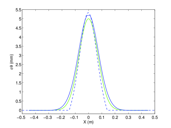
If we are modeling the full dimensional problem in which $\phi=\phi(x,y)$, the damage $\epsilon\theta$ solves a linear partial differential equation of the first order. These differential equations can be solved analytically, but they require a special care in the neighborhood of possible maxima of the temperature where the equation cannot be written in normal form. Although this is still a work in progress, in figure 16 we show the reconstruction of a synthetic damage (green line) detected in 2D with a non constant flux solving a ODE in singular implicit form (continuous blue line) compared with the solution obtained with constant equivalent flux density (dashed line).

In this paper we derive formally an explicit approximation of the solution of a nonlinear inverse problem for the heat equation on a thin conducting plate. More precisely, we recover an inaccessible surface damage $\epsilon\theta$ from thermal data. First we linearize the direct model by means of Domain Derivative. Then, we use perturbation theory in order to construct the Thin Plate Approximation of $\epsilon\theta$ at the first order. Finally, we test the reconstruction strategy with real thermal data.

References

- [1] H. I. Syed, W. Winfree, E. Cramer, P. A. Howell Thermographic Detection of Corrosion in Aircraft Skin in ”Review of Progress in Quantitative Nondestructive Evaluation” DOI: 10.1007/978-1-4615-2848-7, 2035-2041 (1993)
- [2] K. E. Cramer, P. A. Howell, H. I. Syed Quantitative thermal imaging of aircraft structures Proc. SPIE ÒThermosense XVIIÓ, 2473, 226Ð232 (1995)
- [3] J. Hyun Kim, K. Hwan Yoo, M. Gyun Na, J. Weon Kim, K. Suk Kim On-power detection of pipe wall-thinned defects using IR thermography in NPPS Nuclear Engineering and Technology Volume 46, Issue 2, 225Ð234 (2014)
- [4] T. Sakagami, Y. Izumi, Y. Kobayashi, Y. Mizokami, S. Kawabata Applications of infrared thermography for nondestructive testing of fatigue cracks in steel bridges Proc. SPIE 9105, Thermosense: Thermal Infrared Applications XXXVI, 91050S, doi: 10.1117/12.2057382 (2014)
- [5] E. Grinzato, V. Vavilov, P. Bison, S. Marinetti Hidden corrosion detection in thick metallic components by transient IR thermography Infrared Phys. Technol. (49) (2007), pp. 234Ð238
- [6] V. Vavilov, A. Chulkov Detecting corrosion in thick metals by applying active IR thermography Proc. of SPIE, Vol. 8354, 2012, DOI: 10.1117/12.920321
- [7] J V Back, B Blackwell and C A St.Clair, Inverse Heat Conduction - Ill posed Problems Wiley, New York (1985).
- [8] H. T. Banks, F. Kojima and W. P. Winfree, Boundary estimation problems arising in thermal tomography. Inverse Problems 6, 897–921 (1990).
- [9] P.Bison, M.Ceseri, D.Fasino and G.Inglese Domain derivative approach to Active InfraRed Thermography, Inverse Problems in Science and Engineering 18:7, 873-889 (2010).
- [10] K. Brian and L. F. Caudill, Reconstruction of an unknown boundary portion from Cauchy data in dimensions. Inverse Problems 21, 239–255 (2005).
- [11] V. Bacchelli, S. Vessella, Lipschitz stability for a stationary 2D inverse problem with unknown polygonal boundary, Inverse Problems 22, (2006), 1627-1658.
- [12] Bacchelli V, Veneziani A and Vessella S 2010 Corrosion detection in a 2D domain with a polygonal boundary J.Inv.Ill-Posed Problems 18 281-305
- [13] H. S. Carslaw and J. C. Jaeger, Conduction of Heat in Solids. Oxford University Press (1959).
- [14] W.S. Cleveland, Robust Locally Weighted Regression and Smoothing Scatter- plots, J. Amer. Statist. Assoc. 74 (1979), 829–836.
- [15] H. W. Engl, M. Hanke and A. Neubauer, Regularization of Inverse Problems. Kluwer Accademic Publisher (2000).
- [16] D Fasino, G Inglese and F Mariani, Corrosion detection in conducting boundaries: II. Linearization, stability and discretization Inverse Problems 23 (2007) 1101-1114.
- [17] F Hettlich and W Rundell, Identification of a discontinuous source in the heatequation Inverse Problems, Volume 17, Number 5 (2001), 1465-1482.
- [18] G.Inglese, An inverse problem in corrosion detection Inverse Problems 13 (1997), 977–994.
- [19] G Inglese and R Olmi, Nondestructive evaluation of inaccessible surface damages by means of active thermography Rend. Istit. Mat. Univ. Trieste Volume 48 (2016)
- [20] V. Isakov, On uniqueness of obstacles and boundary conditions from the dynamical data, Inverse Probl. Imaging 2 (2008) 151-65
- [21] D.A. Jones, Principles and Prevention of Corrosion Englewood Cliffs, NJ: Prentice -Hall (1996).
- [22] P.G. Kaup, F. Santosa, M. Vogelius. Method for imaging corrosion damage in thin plates from electrostatic data. Inverse Problems, 12 (1996), pp. 279–293.
- [23] X. P. V. Maldague, Theory and Practice of Infrared Technology for Nondestructive Testing. J. Wiley and Sons, (2001), New York.
- [24] S. Salsa, Partial Differential Equations in Action Springer, Milano, 2008.
- [25] Simon J, Differentiation with respect to the domain in boundary value problems, Numer. Funct. Anal. Optim., 2(1980), 649-687.
- [26] COMSOL Multiphysics® v. 5.2. www.comsol.com. COMSOL AB, Stockholm, Sweden.