Bicriteria Rectilinear Shortest Paths among Rectilinear Obstacles in the Plane
Abstract
Given a rectilinear domain of pairwise-disjoint rectilinear obstacles with a total of vertices in the plane, we study the problem of computing bicriteria rectilinear shortest paths between two points and in . Three types of bicriteria rectilinear paths are considered: minimum-link shortest paths, shortest minimum-link paths, and minimum-cost paths where the cost of a path is a non-decreasing function of both the number of edges and the length of the path. The one-point and two-point path queries are also considered. Algorithms for these problems have been given previously. Our contributions are threefold. First, we find a critical error in all previous algorithms. Second, we correct the error in a not-so-trivial way. Third, we further improve the algorithms so that they are even faster than the previous (incorrect) algorithms when is relatively small. For example, for the minimum-link shortest paths, we obtain the following results. Our algorithm computes a minimum-link shortest - path in time. For the one-point queries, we build a data structure of size in time for a source point , such that given any query point , a minimum-link shortest - path can be computed in time. For the two-point queries, with time and space preprocessing, a minimum-link shortest - path can be computed in time for any two query points and ; alternatively, with time and space preprocessing, we can answer each two-point query in time. Note that for any . These results are particularly interesting when is relatively small. For example, if for any , then all above results match the best results for the problems in simple rectilinear polygons, which are optimal. The complexities for the other two types of paths are slightly worse, but still linearly depend on (in addition to for some functions of ).
1 Introduction
Let be a rectilinear domain with a total of holes and vertices in the plane, i.e., is a multiply-connected region whose boundary is a union of axis-parallel line segments, forming closed polygonal cycles (i.e., holes plus an outer boundary). A simple rectilinear polygon is a special case of a rectilinear domain with . A rectilinear path is a path consisting of only horizontal and vertical line segments.
For a rectilinear path , we define its length as the total sum of the lengths of the segments of , and we define its link distance as the number of edges of (each edge is also called a link). We use the measure of to refer to both its length and its link distance. For any two points and in , a shortest rectilinear path from to is a rectilinear path connecting to in with the minimum length, and a minimum-link rectilinear path is a rectilinear - path with the minimum link distance. Among all shortest rectilinear - paths, the one with the minimum link distance is called a minimum-link shortest - path; among all minimum-link - paths, the one with the minimum length is called a shortest minimum-link - path. We define the cost of as a non-decreasing function of both the length and the link distance of . We assume that given the number of links of and the length of , its cost can be computed in constant time. Depending on the context, the measure of may also refer to its cost. A minimum-cost path from to is a rectilinear - path in with the minimum cost (with respect to the cost function ).
All the three types of paths discussed above (i.e., minimum-link shortest paths, shortest minimum-link paths, and minimum-cost paths) are called bicriteria shortest paths. In order to differentiate between “bicriteria shortest paths” and “shortest paths”, we will use optimal paths to refer to these bicriteria shortest paths. Since some observations and algorithmic schemes may be applicable to all three types of optimal paths, unless otherwise stated, a statement made to “optimal paths” should be applicable to all three types of optimal paths.
In this paper, we study the problem of computing all three types of optimal paths between two points and in . Their one-point and two-point queries are also considered.
1.1 Previous Work
These problems have been studied before. The following results are applicable to all three types of optimal paths.
Yang et al. [28] first presented an time algorithm, where is the number of extreme edges of (an edge of is extreme if its two adjacent edges lie on the same side of the line containing ; in the worst case). Later, Yang et al. [29] proposed an algorithm of time and space and another algorithm of time and space; Chen et. al. [6] improved the algorithm to time and space.
The one-point optimal path query problem, where is the source and is a query point, was also studied. Based on the algorithm of Yang et al. [29], Chen et. al. [6] built a data structure of size in time such that for each query point , the measure of the optimal - path can be computed in time and an actual path can be output in additional time linear in the number of edges of the path. For simplicity, in the following, when we say that the query time of a data structure for finding a path is , we mean that the measure of the path can be computed in time and an actual path can be output in additional time linear in the number of edges of the path.
The two-point optimal path query problem, i.e., both and are query points, was also studied by Chen et. al. [6], where a data structure of size was built in time such that each two-point query can be answered in time.
1.2 Our Results
We provide a comprehensive study on these problems. Our contributions are threefold.
First, we show that all the algorithms in the previous work mentioned above are incorrect. More specifically, we find a critical error in the algorithm of Yang et al. [29]. Since the algorithms and data structures of Chen et. al. [6] are all based on the method of Yang et al. [29], the above results of Chen et. al. [6] are not correct either. A similar error also appears in the algorithm of [28]. We should point out that the technique of Chen et. al. [6], which follows the similar idea in Chen et al. [8] for computing shortest paths in arbitrary polygonal domains, would work if it were based on a correct algorithm (for example, it still works in our new algorithm).
Second, we fix the error of Yang et al. [29] in a not-so-trivial way. However, the complexities are not the same as before for all three types of optimal paths. Specifically, for computing a minimum-link shortest path, our corrected algorithm runs in time and space (with the help of the technique of Chen et. al. [6] to reduce a factor of ). For the other two types of optimal paths, however, the complexities have one more factor, i.e., time and space.
Third, we further improve the algorithms in the way that the complexities only linearly depend on (in addition to for some functions of ). For computing a minimum-link shortest path, our algorithm runs in time and space. For computing other two types of optimal paths, our algorithm runs in time and space. We also obtain data structures for one-point and two-point queries. Our results are summarized in Table 1. Note that for two-point queries, we give two data structures for each problem with tradeoff between the preprocessing and the query time. We also consider the two-point query problem for minimum-link paths (without considering the lengths) since the problem was not studied before (but the one-point query problem has already been studied, as discussed below).
Our results are particularly interesting when is relatively small. For example if for any , then for finding a single optimal path of any type, our algorithm runs in time, and our data structures for the minimum-link shortest path and minimum-link path queries are also optimal.
| One-Point Queries | Two-Point Queries | |||
|---|---|---|---|---|
| Min-Link Shortest Paths | Preprocess Time | |||
| Space | ||||
| Query Time | ||||
| Shortest Min-Link Paths | Preprocess Time | |||
| Space | ||||
| Query Time | ||||
| Minimum-Cost Paths | Preprocess Time | |||
| Space | ||||
| Query Time | ||||
| Minimum-Link Paths | Preprocess Time | |||
| Space | ||||
| Query Time | ||||
It is easy to see that the minimum-link shortest paths and the shortest minimum-link paths are special cases of minimum-cost paths, and we discuss them separately mainly because our results for the two special cases are better that those for the minimum-cost paths. In fact, as the cost function is quite general, our algorithm for computing minimum-cost paths may find many applications. We give two examples below.
Polishchuk and Mitchell [24] gave an time algorithm for computing a shortest - path with at most links for a given integer , which improves the time algorithm in [28]. As indicated in [24], the problem can be solved using any algorithm that can find a minimum-cost path with the cost function defined as if and otherwise, where and are the length and the link distance of the path, respectively. Partially due to this reason, Polishchuk and Mitchell [24] already suspected that there is a misunderstanding on the algorithms of [6, 29] for computing minimum-cost paths. We thus confirm their suspicion. On the other hand, applying our new (and correct) algorithm for minimum-cost paths can solve the problem in time, which is faster than the algorithm in [24] when is sufficiently small or when is relatively large.
As a dual problem, finding a minimum-link - path with length at most a given value was also studied in [28], where a worst-case time algorithm was given with as the number of extreme edges of . The problem can also be solved using any minimum-cost path algorithm by defining the cost function as if and otherwise. Hence, applying our algorithm for minimum-cost paths can solve the problem in , which improves the algorithm of [28] since it holds that .
1.3 Other Related Work
If is a simple rectilinear polygon (i.e., ), then there always exists a rectilinear - path that has both the minimum length and the minimum link distance for any two points and in [3, 16]. de Berg [3] built a data structure of size in time that can find such a path in time for any two-point query. The preprocessing time and space were both reduced to by Schuierer [26] (with query time).
If is a general rectilinear domain with , then there may not exist a rectilinear path that is both a minimum-link path and a shortest path [28]. The problems of finding only minimum-link paths or only shortest paths have been studied extensively. Imai and Asano [17] presented an time and space algorithm for finding a minimum-link - path in , and the space was reduced to [14, 21, 25]. Recently, Mitchell et al. [22] proposed an time and space algorithm for the problem, after is triangulated (which can be done in time or time for any [1]). The algorithms in [14, 21, 22] also construct an size data structure that can answer each one-point minimum-link path query in time.
For computing shortest - paths in , Clarkson et al. [11] gave an algorithm of time and space, and as a tradeoff between time and space, they modified their algorithm so that it runs in time and space [12]. Wu et al. [27] proposed an time algorithm, where is the number of extreme edges of , and the algorithm was later improved to time [29]. Mitchell [19, 20] solved the problem in time and space, and Chen and Wang [9, 10] reduced the time to after is triangulated.
If is an arbitrary polygonal domain (i.e., not rectilinear), then the results from [9, 10, 11, 12, 19, 20] are also applicable to finding arbitrary shortest paths under metric. In addition, the algorithms in [9, 10, 19, 20] can be used to compute an size data structure so that each one-point shortest path query can be answered in time. For two-point shortest path queries, Chen et al. [8] constructed a data structure of size in time that can answer each query in time. Recently, Chen et al. [7] reduced the query time to by building a data structure of size in time.
To find a minimum-link - path between two points and in an arbitrary polygonal domain , Mitchell [23] gave an time algorithm, where is the inverse of Ackermann’s function and is the size of the visibility graph of and in the worst case. The one-point query problem was also studied in [23].
In the following, unless otherwise stated, a path always refers to a rectilinear path.
1.4 Our Techniques
Given two points and in the rectilinear domain , to find an optimal - path, the algorithm of Yang et al. [29] first built a “path-preserving” graph of size by using the idea of Clarkson et al. [11]. Then, it is shown that contains an - path that is homotopic to an optimal - path in with the same length, and further, can be obtained from by performing certain “dragging” operations. Motivated by this observation, Yang et al. [29] computed an optimal - path by applying Dijkstra’s algorithm on and simultaneously performing the dragging operations. We find a critical error in their way of applying Dijkstra’s algorithm. We fix the error by using a “path-based” Dijkstra’s algorithm and maintaining some additional information, and we prove that our algorithm is correct. Due to that we need to maintain more information on computing shortest minimum-link paths and minimum-cost paths, our algorithm for them runs slower than that for computing minimum-link shortest paths.
To further reduce the running time (for small ), our main idea is to use a reduced graph of size instead of . We show that contains an - path that is homotopic to an optimal - path in with the same length, and further, can be obtained from by performing the dragging operations as in [29] and a new kind of operations, called through-corridor-path generating operations. The graph is built based on a corridor structure of , which was used to find minimum-link paths in [22]. More specifically, we decompose into junction rectangles and corridors. Each corridor is a simple rectilinear polygon. Although each corridor may have vertices, we show that we only need to consider at most four points of each corridor to build the graph . To this end, we make use of the histogram partitions of rectilinear simple polygons [26].
To solve the one-point queries, the approach of Chen et al. [6] is to “insert” the query point to the graph to obtain a set of vertices (called “gateways”) of such that an optimal path can be obtained by performing the dragging operations from the gateways. We follow the similar scheme but on our reduced graph , where only gateways are necessary. Further, we also need to utilize the techniques of Schuierer [26] for simple rectilinear polygons.
For the two-point queries, the approach of Chen et al. [6] inserts both query points and to the graph to obtain a set of gateways for and a set of gateways of for , so that an optimal - path can be obtained by performing the dragging operations from these gateways. The query time becomes because every pair of points with and needs to be considered. We again use the same scheme but on the graph with only gateways for both and , which reduces the query time to . To further reduce the query time to , we follow the scheme in [7] for solving two-point shortest path queries in arbitrary polygonal domains. The main idea is to build a larger graph by adding more vertices to such that gateways are sufficient for each query point.
The rest of the paper is organized as follows. We introduce some notation and concepts in Section 2. In Section 3, we review the algorithm given by Yang, Lee, and Wong [29] (we refer to it as the YLW algorithm), point out the error, and correct it. In Section 4, we further improve the algorithm for finding a single optimal - path. The one-point and two-point path query problems are discussed in Sections 5 and 6, respectively.
2 Preliminaries
In this section, we define notation and review some concepts. Some terminologies are borrowed from the previous work, e.g., [7, 8, 11, 29]
For any two points and of , if the line segment is in , then we say that is visible to . Consider a vertical line and a point . Let be the point on whose -coordinate is the same as that of . We call the horizontal projection of on . If is visible to , then we say that is horizontally visible to .
For any two points and , we use to denote the rectangle with as a diagonal. A path in is L-shaped if it consists of a horizontal segment and a vertical segment (each of them may be empty). A path is U-shaped if it consists of three segments , , and such that and are on the same side of the line containing (e.g., see Fig. 1). A path is called a staircase path if it does not contain a U-shaped subpath. Note that a staircase path is a shortest path.

Let denote the set of all vertices of . We let also include the two points and . We review a path-preserving graph on , which was originally from [11] and has been used elsewhere, e.g., [7, 8, 18, 29]. The vertex set of consists of the points of and Steiner points on some vertical lines, called cut-lines. The cut-lines and the Steiner points are defined as follows.
Let be the point of with the median -coordinate. The vertical line through is a cut-line. For each point , if is horizontally visible to , then the horizontal projection of on is a Steiner point. Let (resp., ) be the points of on the left (resp., right) side of . The cut-lines and Steiner points on the left and right sides of are defined on and , recursively. We use a binary tree to represent the above recursive procedure, called cut-line tree. Each node corresponds to a cut-line and a subset . If is the root, then is and . The left and right subtrees of the root are defined recursively on and . Hence, has nodes and each point of can define a Steiner point on at most cut-lines. Therefore, there are Steiner points in total.
The vertex set of consists of all points of and all Steiner points defined above. The edges of the graph are defined as follows. First, if a point defines a Steiner point on a cut-line, then has an edge . Second, for any two adjacent Steiner points and on each cut-line, if the two points are visible to each other, then has an edge .
Clearly, has nodes and edges. Each edge of the graph is either horizontal or vertical. Each edge of has a weight that is the length of the corresponding line segment. The graph can be built in time [11, 18, 29]11 1 The graph introduced in [11] also includes Steiner points on horizontal cut-lines and projection points of on the boundary of . However, in our problem, since is rectilinear, by the similar analysis as in [11], we can show that our graph is also a path-preserving graph. We will give analysis details when we prove a similar observation on our reduced graph in Section 4.3 (i.e., Lemma 3 and Corollary 1).. The following lemma will be useful later.
Lemma 1
For any path in , let denote its length and let denote its link distance. For any two points and on , if the context is clear, we often use to denote the subpath of between and . For any two points and in the plane, we say that is to the northeast of if is in the first quadrant (including its boundary) with respect to . Similarly, we define northwest, southwest, and southeast.
3 The YLW Algorithm and Our Correction
In this section, we first review the YLW algorithm [29] and then point out the error. Finally, we will fix the error and prove the correctness our new algorithm.
3.1 The YLW Algorithm
The YLW algorithm is essentially based on the following observation.
Lemma 2
(Yang et al. [29]) For any optimal path from to in , there is path in such that and is homotopic to (i.e., can be continuously dragged to without going outside of ).
We briefly review the proof of Lemma 2 because it will help to understand the algorithm and also help us to prove the correctness of our new algorithm given later.
Let be any optimal path from to . It is shown (Lemma 2.1 [29]) that can be divided into a sequence of staircase subpaths, and the two endpoints of each such subpath are in . Hence, it is sufficient to prove the lemma for any staircase subpath of . In the following, we consider a staircase subpath of with and as the two endpoints. We further obtain a pushed staircase path as follows. Without loss of generality, we assume is to the northeast of and the segment of incident to is horizontal. We push the first vertical segment of rightwards until either it hits a vertex of or it becomes collinear with the second vertical segment of . If the latter case happens, then we merge the two vertical segments and keep pushing the merged vertical segment rightwards. If the first case happens, then we push the next horizontal segment upwards in a similar way. The procedure stops until we arrive at the segment incident to . Let denote the resulting path. Observe that , is homotopic to , and is also a staircase path. is called a pushed staircase path [29]. Also note that each segment of contains at least one vertex of .
Remark.
There are eight types of pushed staircase paths from to depending on which quadrant of the point lies in and also depending on whether the first segment of the path incident to is horizontal or vertical.
The vertices of partition into subpaths. To prove the lemma, it is sufficient to show the following claim: for any subpath of between any two adjacent vertices and of on , there is a path connecting and in with the same length and the two paths are homotopic. Because every segment of contains at least one vertex of , must be an L-shaped path. Without loss of generality, we assume is to the northwest of . If the rectangle is empty (this includes the case where is a single segment), then by Lemma 1, the above claim is true. Otherwise, as shown in [29] (Lemma 4.5), there are some points of in that can be ordered as with being empty and to the northwest of for each , and further, is homotopic to the concatenation of for all . By Lemma 1, for each , contains a staircase path connecting and and the path is in (and thus is homotopic to ). Therefore, by concatenating the staircase paths from to for all , we obtain a staircase path from to and the path is homotopic to . Note that the staircase path has the same length as since is an L-shaped path (and thus is also a shortest path). The above claim thus follows.

This proves Lemma 2. The proof actually constructs the path in corresponding to the optimal path , and is called a target path. Yang et al. [29] also showed that can be obtained from by applying certain dragging operations during searching the graph . Before describing the details of the operation, we first give some intuition on how can be obtained from . Based on the above constructive proof for Lemma 2, we only need to show that for each L-shaped path , it can be obtained from the corresponding staircase path in . Without loss of generality, we assume that is to the northeast of and the segment incident to in is vertical. Because is homotopic to , we can convert to as follows (e.g., see Fig. 2). Starting from , for each horizontal segment of , drag it upwards until either it hits the horizontal segment of or it becomes collinear with the next horizontal segment of . In the former case, we have obtained . In the latter case, we continue to drag the new horizontal segment upwards in the same way as before.
In the sequel, we briefly review the dragging queries [29]. This will make our paper self-contained and also help us to explain our new algorithm as well as the optimal path queries given later.
The YLW algorithm intends to search a target path in . The algorithm starts from . When a vertex of is processed, at most eight paths from to are stored at such that their last pushed staircase subpaths containing are different. Later the algorithm will advance these paths from to each neighboring vertex of in . Let be such a path stored at and we want to advance it from to to obtain a path from to . Without loss of generality, we assume is to the northeast of , where is the start point of the last staircase path of containing , and we also assume that the last segment of is horizontal (i.e., is incident to ). Other cases are similar. Let . We obtain from by a dragging operation on as follows. We say that is fixed if it borders an obstacle that is above , in which case cannot be dragged upwards anymore, and is floating otherwise. Since is an edge of , it is either vertical or horizontal.

- 1.
If is to the right of , then and the last segment of is .
- 2.
If is to the left of , then we ignore the path (i.e., the path will not be considered).
- 3.
If is above (i.e., is vertical), then depending on whether is fixed there are two subcases.
- (a)
If is fixed (e.g., see Fig. 3(a)), then and becomes the last segment of . Note that is fixed if and only if it borders an obstacle that is on its right side.
- (b)
If is floating, then there are further two subcases.
- i.
If can be dragged upwards to without hitting a point of (e.g., see Fig. 3(b)), then we drag to and obtain , which has the dragged as its last segment.
- ii.
Otherwise, we ignore the path .
- i.
- (a)
- 4.
If is below , then there are further two subcases.
- (a)
If borders an obstacle below it (e.g., see Fig. 3(c)), then a new U-shaped path is generated and a new pushed staircase subpath is also generated with being the first segment. We have with as the last segment.
- (b)
Otherwise, we ignore the path .
- (a)
If we apply the dragging operations on a target path from to , then an optimal path can be eventually produced. This can be seen from the intuition we discussed earlier (refer to Lemma 4.6 of [29] for details). This motivates the YLW algorithm, which we describe below on finding a minimum-link shortest - path (other two types of optimal paths are similar).
The YLW algorithm works by applying Dijkstra’s algorithm according to the measure vector for a path . Initially, all vertices of are in a priority queue with measure vectors except that the measure vector for is . As long as is not empty, the algorithm removes from the vertex with the smallest measure vector (lexicographically, i.e., for two vectors and , the first one is smaller than the second one if and only if , or and ) and advance the paths stored at to each of ’s neighbor by using the dragging operations. Let be a path obtained for . There may be other paths that are already stored at and the types of the last staircase subpaths of these paths are also stored (recall that there are eight types of pushed staircase subpaths). The YLW algorithm relies on the following two rules to determine whether the new obtained path should be stored at , and if yes, whether some paths stored at should be removed. Let be any path that has already been stored at .
- Rule()
If the measure vectors of and are not the same, then discard the one whose measure vector is strictly larger.
- Rule()
If and have the same measure vector and of the same type, compare their last segments. If their last segments overlap, discard the path whose last segment is longer.
It is claimed in [29] that once the point is processed, among all paths stored at , the one with the smallest measure vector is an optimal - path.

We find that the algorithm is not correct, mainly due to Rule(). Figure 4 illustrates a counterexample. Assume that both and are paths from to with and . Thus, the measure vector of is strictly smaller than that of . According to Rule(), we should discard . Observe that we can obtain an - path from to using without having any extra link. However, to obtain an - path using , we need at least two more links. Therefore, can lead to a better - path than , and thus, we should not discard . Notice that the reason this happens is that although the measure vector of is strictly smaller than that of , the last segment of is shorter than that of (and thus it may be “freely” dragged upwards higher than that of ).
In fact, the most essential reason for this error to happen might be the following. If is a shortest - path, then for any two points and in , the subpath of between and is also a shortest path from to . However, this may not be the case for minimum-link paths. Namely, if is a minimum-link - path, then it is possible that for two points and in , the subpath of between and is not a minimum-link path from to . Due to this reason, one can verify that the time algorithm given by Yang et al. [28] for computing optimal paths is not correct either. Indeed, the approach in [28] also applies Dijkstra’s algorithm on a graph to search the optimal paths using the measure vectors like .
3.2 Our New Algorithm
To fix the error, we need to fix Rule(). We first consider the minimum-link shortest paths. We replace Rule() by the following Rule(), but still keep Rule(). (Recall that denotes any path that has already been stored at .)
- Rule()
Let be one of and , and the other. If , or but , then we discard .
By Rule(), we may need to store two paths and at even if the measure vector of one path is strictly smaller than that of the other, in which case and . Hence, unlike the YLW algorithm, each vertex of may store paths with different measure vectors. Therefore, we cannot apply the same “vertex-based” Dijkstra’s algorithm as before. Instead, we propose a “path-based” Dijkstra’s algorithm. Roughly speaking, we will process individual paths instead of vertices. Specifically, in the beginning there is only one path from to itself in the priority queue . In general, as long as is not empty, we remove from the path with the smallest measure vector. Assume that the endpoint of is . Then, we advance from to each of ’s neighbors . If is stored at by our rules (i.e., both Rule() and Rule()), then we (implicitly) insert to . The algorithm stops once is empty. Since we process paths following the increasing measure order, the algorithm will eventually stop. Finally, among all paths stored at , we return the one with the smallest measure as the optimal solution.
We will prove the correctness of the algorithm in Section 3.3. In terms of the running time, the YLW algorithm maintains at most eight paths at each vertex of . To see this, due to the Rule(), for each type of staircase paths, maintains at most one path. In our new algorithm, the paths maintained at always have the same length but their link distances differ by at most one. Hence, again due to Rule(), there are at most sixteen paths maintained at . Clearly, this does not affect both the time and the space complexities of the algorithm asymptotically. Thus, the algorithm still runs in time and space, as the YLW algorithm.
In addition, using another path-preserving graph of vertices and edges [12], Yang et al. [29] proposed another time and space algorithm (see Section 4.2 of [29]). Further, Chen et al. [6] reduced the space of the algorithm to with the same time (similar technique was also used in [8]). By applying the techniques of both [29] and [6] to our new method, we can also obtain an algorithm of time and space. We omit the details.
We proceed on the problem of finding a minimum-cost - path. Recall that we have a cost function . For any path , we use to denote the cost of the path. Our algorithm is the same as above with the following changes. First, the paths in the priority are prioritized by . Second, we replace both Rule() and Rule() by the following rule.
- Rule()
Let be one of and , and the other. If the last segments of and are exactly the same and , then we discard .

We give some intuition on why we use the above rule. Refer to Fig. 5, where there are three paths , , and from to . Let be the last segment of for each , and we assume that they overlap with , where is the length of each . We also assume that and . In this case, we have to keep all three paths because any of them may lead to the best path from to . For example, for each , the path may lead to the best path from to . One can generalize the example so that a total of paths may need to be stored at . However, is the upper bound since the last segment of each such path starts from a different vertex of in the horizontal line through and there are such vertices. For this reason, their are paths stored in all vertices of . Hence, the running time of the algorithm becomes and the space becomes . One may want to use some other rules to reduce the number of paths that need to be stored at , e.g., Rule(); however, in the worst case, the number of paths stored at is still .
We point out a detail about the algorithm implementation. Suppose we have computed a new path at and we want to apply Rule. Then, we need to know whether there is a path already stored at whose last segment is exactly the same as that of . If we check every path stored at , then this step would cost time, resulting in an overall time. We can actually implement this step in time, as follows. Let be the last segment of and suppose is horizontal. Observe that must be a vertical projection of a point in on the horizontal line through . We use an array of size such that corresponds to the -th vertex of in the order of increasing -coordinate. Hence, if is the projection of the -th vertex of , then we can simply check the path stored at in time, and if should be stored, then we simply store it at . Similarly, we also build another array for the horizontal projections of the vertices of on the vertical line through . In this way, the overall running time of the algorithm is . The space complexity is still because the total size of the arrays at each vertex of the graph is .
Further, as for the minimum-link shortest paths, by using the graph and the techniques in [6, 29], we can reduce the running time by a factor of . We omit the details.
For computing a shortest minimum-link - path, we use the same algorithm as above for the minimum-cost paths but with the following changes. First, we use the measure vector instead. Second, we use the following rule, which is similar to Rule().
- Rule()
Let be one of and , and the other. If the last segments of and are exactly the same and the measure vector of is no larger than that of , then we discard .
The time and space complexities are the same as the above for the minimum-cost paths.
If we are looking for a minimum-link - path (without considering the length), then we can use the following rule.
- Rule()
Let be one of and , and the other. If , then we discard . We also discard if the following is true: , the last segments of and overlap, and the last segment of is no longer than that of .
The rule makes sure that we only need to keep at most eight paths at any vertex of : for each of the following four directions of : left, right, above, below, there are two paths whose last segments are from that direction and their link distances differ by at most one. Hence, similar to the minimum-link shortest paths, we can find a minimum-link path in time and space. As discussed in Section 1, the problem of finding a single minimum-link path and its one-point query problem have been solved optimally [22] (after is triangulated). We discussed the above result mainly because we will use it to answer the two-point queries in Section 6.
The correctness of all above algorithms is proved in Section 3.3.
3.3 The Correctness of Our Algorithm
We first show the correctness of the algorithm for computing a minimum-link shortest path. The analysis for other paths is very similar.
Let be a minimum-link shortest - path in . Let be the corresponding target path from to in the graph . For any vertex in the target path, let be the path in from to obtained by applying the dragging operations on the subpath of from to . To prove the correctness of our algorithm, it is sufficient to show that the paths of for the vertices of from to will be computed and advanced following the vertex order of during our algorithm. According to our analysis before, we only need to prove it for any L-shaped subpath between two adjacent vertices and of .
We assume the path has been computed and stored at , and is about to advance. Initially this is trivially true when . Let be the subpath of between and , and let be the vertices of in order from to . Recall that is a staircase path. Without loss of generality, we assume is to the northeast of . If the path is stored at , then our algorithm is correct. Otherwise, there must be a path stored at that causes not to be stored. According to Rules and , at least one of the following cases must happen: (1) ; (2) but ; (3) the measure vectors of the two paths are exactly the same, the last staircase subpaths of both paths are of the same type, and the last segment of is shorter than or equal to that of .
If Case (1) happens, then consider the following path from to (e.g., see Fig. 6): the concatenation of , a vertical segment from to a point on the horizontal segment of the L-shaped subpath , and the subpath of between and . Note that . Because (i.e., Case (1)) and , we obtain , contradicting with that is a shortest path.

If Case (2) happens, then we still consider the path obtained above. Observe that , where the minus 1 is due to that we may be able to drag the last segment of so that it overlaps with the first segment (and thus save one link). Also note that , where the plus 1 is due to the segment . Since (i.e., Case (2)), we obtain that . Further, because , we obtain . This implies that using we can also obtain a minimum-link shortest - path, and thus, can be safely ignored.
If Case (3) happens, then similar to the proof of Lemma 4.7 in [29], using we can also obtain a minimum-link shortest - path, and thus, can be safely ignored.
The above proves that in any case our algorithm stores necessary paths at that can be used to eventually obtain a minimum-link shortest - path. By the similar argument, we can show that this is true for for all . This establishes the correctness of our algorithm.
We proceed to show the correctness of our algorithm for computing a minimum-cost - path. We follow the above analysis scheme and focus on proving that the path will be stored at if necessary. If is not stored at , then according to Rules , this only happens because there is another path stored at such that the last segments of and are exactly the same and .
First of all, we know that the last segment of (i.e., ) is horizontal and we can drag it upwards freely until the horizontal segment of the L-shaped path to obtain the path (i.e., by concatenating with ). Since the last segments of and are exactly the same, regardless of whether and are of the same type, we can also drag the last segment of upwards freely until , so that we can obtain another - path . Further, the above dragging on the last segment of does not introduce any extra link and the amount of length it introduces is the same as that introduced by dragging the last segment of . As and the cost function is non-decreasing in both the length and the link distance of the path, we can obtain that . Hence, we can also obtain a minimum-cost - path by using , and thus can be safely ignored without being stored at . This establishes the correctness of the algorithm.
The correctness of our algorithm for computing shortest minimum-link paths follows the similar analysis as the above case for minimum-cost paths. We omit the details.
Finally, we show the correctness for computing a minimum-link - path. We again follow the above scheme. If the path is not stored at , then according to Rule , there must be another path stored at such that one of the following two cases happens: (1) ; (2) , the last segments of both paths overlap, and the last segment of is no longer than that of the last segment of .
If Case (1) happens, then as in the analysis for minimum-link shortest paths, we consider the path obtained from by adding a vertex segment . We have shown above that and thus it is safe to ignore . If Case (2) happens, we can follow the proof of Lemma 4.7 of [29] (or the similar analysis as the above for the minimum-cost paths) to show that can also lead to a minimum-link - path.
4 The Improved Algorithm
In this section, we improve our algorithm proposed in Section 3, so that in addition to , the complexities of our improved algorithm only depend on , i.e., the number of holes of . We first review the corridor structure of [22] and the histogram partitions of rectilinear simple polygons [26].
4.1 The Corridor Structure of
For ease of exposition, we make a general position assumption that no two edges of are collinear. The vertical visibility decomposition of , denoted by , is obtained by extending each vertical edge of until it hits the boundary of (e.g., see Fig. 8). Each cell of is a rectangle. Each extension segment is called a diagonal of .


The corridor structure of has been introduced before, e.g., see [22]. Let be the dual graph of (e.g., see Fig. 8), i.e., each node of corresponds to a cell of and two nodes have an edge if the corresponding cells share an edge. Based on , we obtain a corridor graph as follows. First, we keep removing every degree-one node from along with its incident edge until no such nodes remain. Second, we keep contracting every degree-two node from (i.e., remove the node and replace its two incident edges by a single edge) until no such nodes remain. The graph thus obtained is , which has nodes and edges [22]. Refer to Fig. 8 for an example. The cells of corresponding to the nodes of are called junction rectangles. If we remove all junction rectangles from , each connected region is a simple rectilinear polygon, which is called a corridor. Each corridor has two diagonals each of which is on a vertical side of a junction rectangle, and we call them the doors of the corridor. For convenience, if a diagonal bounds two junction rectangles (e.g., see Fig. 8), then we consider itself as a “degenerate” corridor whose two doors are both . With the degenerated corridors, each vertex of lies in a unique corridor.
The decomposition can be computed in time for any [1]. After is known, the corridor structure of (i.e., computing all corridors and junction rectangles) can be obtained in time.
4.2 The Histogram Partitions
The histogram partition is a decomposition of a simple rectilinear polygon [26]. We will need to build the histogram partitions on the corridors of . Below we review the partition and we follow the terminologies of [26].
A simple rectilinear polygon is called a histogram if its boundary can be divided into an - or -monotone chain and a single line segment; the single segment is called the base of (e.g., see Fig. 10).


Consider a simple rectilinear polygon (e.g., a corridor of the corridor structure of ) and let be an edge of (e.g., a door of ). A histogram partition of with respect to , denoted by , is defined as follows. Let be the maximal histogram with base in , i.e., there is no other histogram in with base that can properly contain it (e.g., see Fig. 10). A window of is a maximal segment on the boundary of that is contained in the interior of except its two endpoints (e.g., see Fig. 10). For each window of , it divides into two subpolygons, and we let denote the one that does not contain . If does not have a window, then we are done with the histogram partition of . Otherwise, for each window , we perform the above partition on recursively with respect to .
4.3 A Reduced Path Preserving Graph
Recall that our algorithm in Section 3 use a graph , which is built on the vertices of and has nodes and edges. In this section, as a major tool for reducing the complexities of our algorithm, we propose a reduced graph of only nodes and edges.
The rest of this section is organized as follows. In Section 4.3, we introduce a set of backbone points, based on which we will define the reduced graph in Section 4.3. In Section 4.3, we compute . In Section 4.4, we give an algorithm to compute optimal paths by using , and Section 4.5 proves its correctness. The algorithm in Section 4.4 is for the special case where both and are in junction rectangles. Section 4.6 generalizes the approach to other cases.
The Backbone Points
We introduce a set of backbone points on the doors of the corridors of , which will be used to define our reduced graph later.
Consider a corridor of the corridor structure of . Let and be the two doors of . Note that both doors are vertical. The region of excluding the two doors is called the interior of . If there exist a point and a point such that is horizontal and in then we say that is an open corridor; otherwise, it is closed (e.g., see Fig. 12 and Fig. 12).


Consider an open corridor (e.g., see Fig. 12). Let and be the points defined above. Imagine that we drag vertically upwards (resp., downwards) until we hit a vertex of , then the current locations of and are two backbone points. In this way, each door of has two backbone points. Clearly, the rectangle with the four backbone points as the vertices is in and we call the canal of . The two horizontal edges of are called bridges of . Further, the top edge of is the upper bridge and the bottom edge is called the lower bridge.
If is a degenerate corridor, which is a single diagonal , then is also an open corridor and the upper (resp., lower) bridge is degenerated to the upper (resp., lower) endpoint of .
We have the following self-evident observation on open corridors.
Observation 1
Suppose and are the two doors of an open corridor . Consider any two points and .
- 1.
If both and are on the boundary of the canal , then is a shortest path in from to , where is the horizontal projection of on .
- 2.
Otherwise, is a shortest path in from to for some bridge of .
In either case, we use to denote the above shortest path between and , and we call it a canonical path.
Next, we consider the case where is closed (e.g., see Fig. 12). Let be the maximal histogram in with base . As is closed, has a window that separates from , that is, divides into two sub-polygons that contain and , respectively. By the definition of windows, if we extend to , the extension will hit at a point, denoted by , before it goes out of . Similarly, we define , , and , with respect to the other door . The two points and are backbone points of . The following is proved in [26].
Observation 2
(Lemma 3.1 of [26]) Suppose and are the two doors of a closed corridor . For any two points and , the concatenation of , a shortest path from to in , and is a shortest path from to in . We use to denote the path, and we call it a canonical path.
The above defines two backbone points on each door of every open corridor and one backbone point on each door of every closed corridor. Let denote the set of all such backbone points. Since there are corridors, the size of is .
The Reduced Graph
In the following, we introduce the reduced graph, denoted by , and we will use it to compute optimal paths. We first consider the case where both and are in junction rectangles. With a little abuse of notation, we let also contain both and .
We build the graph with respect to the points of in the same way as with respect to in Section 3. Hence, has vertices and edges. In addition, we add the following edges to . Consider a closed corridor with the two backbone points and on its two doors. Note that and are also two vertices in . We add to an edge to connect and with length equal to , i.e., the length of the canonical path . We call a corridor edge of , and call a corridor path of . We do this for all closed corridors. This completes the construction of . Since there are corridors, has corridor edges. For differentiation, other edges of that are not corridor edges are called ordinary edges. Hence, has edges in total.
Note that every path in corresponds to a path in with the same length in the sense that if the path contains a corridor edge, then contains the corresponding corridor path. Similar to Lemma 1, we have the following observation.
Observation 3
For any two points and in , if the rectangle is empty, then contains a staircase path connecting and .
The following lemma is analogous to Lemma 2, but on the reduced graph . It explains why the graph can help to find optimal paths.
Lemma 3
There exists a path in from to that is homotopic to an optimal - path and the two paths have the same length; we call a target path.
Proof
Let be an optimal - path in . Since both and are in junction rectangles, an easy observation is that if contains an interior point of a corridor , then must travel through , i.e., enters through one door and leaves through the other.
We assume that travels through some closed corridors since otherwise the analysis would be similar (but easier). Consider each such closed corridor with two doors and . Let and be the two backbone points on and , respectively. If we traverse from to , define to be the last point on we encounter and define to be the first point on we encounter. Hence, the subpath of between and , denoted by , is in . We obtain another - path by replacing with the canonical path in . By Observation 2, is a shortest path in , and thus, . Since both and are paths in , which is simply connected, they are homotopic to each other. Therefore, is homotopic to . Note that contains the two backbone points and and the subpath of between and is the corridor path of , which corresponds to a corridor edge in .
We do the above for all such closed corridors that are traveled through by . With a little abuse of notation, let be the new - path. By the above analysis, and is homotopic to . Let be a maximal subpath of that does not contain any corridor path. Note that does not contain an interior point of any closed corridor. Let and be the two endpoints of . Clearly, and are in . Because all corridor paths are in , to prove the lemma, it is sufficient to show that there is a path in connecting and with the same length as and the path is homotopic to . We assume that travels through at least one open corridor since otherwise the analysis would be similar (but easier).
Suppose travels through an open corridor . If we traverse on from to , let be the first point and last point of , respectively. Hence, is on a door of and is on the other door. Let be the subpath of between and . We obtain another path from to by replacing with the canonical path . Since is a shortest path between and in , and is homotopic to . By Observation 1, consists of at most one horizontal segment and at most two vertical segments, and further, the two endpoints of the horizontal segment are on the two doors of , respectively, and the two vertical segments are on the doors of .
We do this for all such open corridors that are traveled through by . Let denote the new path, which still connects and . Based on the above discussion, and is homotopic to . Further, for each horizontal segment of , if it intersects the interior of a corridor (which is necessarily an open corridor), then it must intersect both doors of .
Suppose we traverse from to . If intersects a junction rectangle , then let and be the first and last points intersecting , respectively. Let be the subpath of between and . We obtain another path from to by replacing with an L-shaped path connecting and , which has the same length as and is homotopic to . Hence, has the same length as and is homotopic to .
We do the above for all such junction rectangles intersected by , and let be the resulting path, which still connects to . The length of is the same as that of and is homotopic to . Further, for each vertical segment of that is not incident to either or , it must be on a vertical side of a junction rectangle.
We assume that contains a U-shaped subpath since otherwise the analysis would be similar (but easier). Consider a U-shape subpath of with three segments , , and . As shown in [29], must contain an obstacle edge of since otherwise we could shorten the path by dragging towards the direction of and . Depending on whether is horizontal or vertical, there are two cases.
- 1.
If is horizontal, then must intersect the interior of an open corridor . To see this, on the one hand, cannot be in a closed corridor because (and thus and ) does not contain an interior point of any closed corridor. On the other hand, the top or bottom side of each junction rectangle only contains a proper subset of an obstacle edge.
Since is a horizontal segment of and (and thus ) intersects the interior of , intersects both doors of , say, at two points and . Without loss of generality, we assume the obstacle bounded by is locally above . Because intersects the interior of and is an obstacle edge, we cannot freely move in vertically upwards. This implies that is the upper bridge of and thus and are two backbone points of . We pick either one of and , and call it a breakpoint of .
- 2.
If is vertical, since is between and , cannot be incident to either or . Hence, (and thus ) must be on a vertical side of a junction rectangle . Further, since and are toward the same direction, each of and must go inside an open corridor from since otherwise they would have to both go inside and we could drag to shorten the path.
Let be the common endpoint of and (e.g., see Fig. 13). Hence, must be on a door of an open corridor . Since goes inside , must also intersect the other door of . Without loss of generality, we assume is above . Since contains an obstacle edge , and are on the same side of and is higher than . As intersects both doors of , it must be higher than the lower bridge of . This implies that must contain the endpoint of the lower bridge of on , and we call a breakpoint of .

In either case above, we show that must contain a backbone point as a breakpoint of .
If has other U-subpaths, then for each of them, the middle segment also contains a backbone point as a breakpoint of . Hence, if is a subpath of partitioned by the breakpoints, then must be a staircase path and both endpoints of must be in . Let and be the two endpoints of , respectively. To prove the lemma, it is sufficient to show that has a path connecting and with the same length as and the path is homotopic to .
Without loss of generality, we assume that is to the northeast of . Based on , in the following, we obtain another shortest path from to such that has the same length as and is homotopic to . In fact, is similar in spirit to the pushed staircase path defined in [29] (also discussed in Section 3) but with respect to the open corridors and the junction rectangles. If the segment of incident to is horizontal, then let be the second horizontal segment of ; otherwise let be the first horizontal segment of . Unless is incident to , we push upwards until either it hits a vertex of or it becomes collinear with the next horizontal segment of . In the latter case, we merge the two horizontal segments and let refer to the merged segment and we push upwards again. This procedure stops either when hits an edge of or becomes incident to . We do the same for the rest of horizontal segments following their order along the path from to . Let denote the resulting path. Clearly, has the same length as and is homotopic to .
Next, we push the vertical segments of . If the segment of incident to is vertical, then let be the second vertical segment of ; otherwise let be the first vertical segment of . Unless is incident to , we push rightwards until either it hits a vertex of or it becomes collinear with the next vertical segment of . In the latter case, we merge the two vertical segments and let refer to the merged segment and we continue to push rightwards. This procedure stops either when hits a vertex of or becomes incident to . Suppose hits a vertex of . If is on the boundary of a junction rectangle , in which case is on the right side of , then we do nothing. Otherwise, must be a vertex in the interior of an open corridor , in which case we push leftwards until it overlaps with the left door of (note that is now on the right side of a junction rectangle). This finishes the push operation for the vertical segment . We proceed to do the same for the rest of the vertical segments following their order along the path from to . Let be the resulting path. Clearly, has the same length as and is homotopic to .
Consider any segment of . In the following, we show that must contain a backbone point of . This is obviously true if is incident to either or . Below we assume that is incident to neither nor . Depending on whether is horizontal or vertical, there are two cases.
- 1.
If is horizontal, then contains an obstacle edge that bounds an obstacle from below. Recall that due to definition of degenerated open corridors, each vertex of must be in a corridor. Let be the corridor that contains the right endpoint of . Note that may be a degenerated open corridor. Since both the vertical segments of right before and after are on vertical sides of junction rectangles, must travel through . Further, contains the upper bridge of since the portion of between the two doors of cannot be dragged upwards in due to . Hence, contains two backbone points that are the two endpoints of the upper bridge of .
- 2.
If is vertical, then according to our construction of , is on the right side of a junction rectangle. Depending on whether contains an obstacle vertex, there are two cases.

Figure 14: The blue dashed dotted path is , where the two segments and are labeled. The red dotted segment is the lower bridge of . 
Figure 15: The upper and lower endpoints of are and , respectively. The obstacle vertex is also labeled. - (a)
If contains an obstacle vertex, let be the upper endpoint of (e.g., see Fig. 15). Then, the next horizontal segment of starts from going rightwards inside an open corridor , and this segment travels through . Let be the door of that contains . Let be the lower endpoint of . Since contains an obstacle vertex and the upper endpoint of is on , must be on . Further, since travels through , must contain the left endpoint of the lower bridge of , which is a backbone point. As , contains the above backbone point.
- (b)
Otherwise, according to our construction of , if we push rightwards, then we will hit an obstacle vertex in the interior of (e.g., see Fig. 15). Let be the next horizontal segment of . As the above case, is going rightwards and travels through . This means that is below . Note that the lower bridge of must be below and above . Also note that overlaps with the left door of . Let and be the upper and lower endpoints of , respectively. Since will be hit if we push rightwards, is above and below . Since is above and below (and thus ), we obtain that is above and below (e.g., see Fig. 15). Therefore, the left endpoint of , which is a backbone point, is on . This proves that contains a backbone point.
- (a)
The above shows that each segment of contains a backbone point. Hence, each subpath of partitioned by all breakpoints on must be an L-shaped path. Let be any such subpath, and let and be its endpoints, which are both in . To prove the lemma, it is sufficient to show that contains a path from to that has the same length as and is homotopic to , as follows.
Without loss of generality, we assume is to the northeast of . We also assume that the segment incident to is horizontal and the one incident to is vertical. Other cases can be analyzed similarly. Hence, consists of a horizontal segment and a vertical segment for some point .
If the rectangle is empty (i.e., in ), then by Observation 3, contains a staircase path from to in . Since is in , is homotopic to with the same length. Otherwise, there exist backbone points contained in and they can be ordered as such that is to the northeast of and is empty for each . By Observation 3, for each , since the rectangle is empty, has a staircase path from to . Let be the concatenation of all these staircase paths for . Clearly, is a staircase path and thus has the same length as . In the following, we show how we find the above sequence of backbone points, and the way we find them will also imply that is homotopic to .
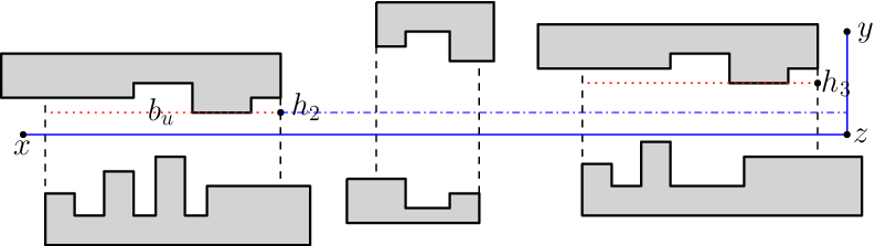
Since is vertical and is in a junction rectangle, is also in the same junction rectangle. Refer to Fig. 16. As is not empty and both and are in junction rectangles, must travel through some open corridors (maybe degenerated). We push upwards until it hits a vertex of , at which moment, the new segment, denoted by , must contain the upper bridge of an open corridor, and we let refer to the right endpoint of (recall that ). Note that is to northeast of of and is empty. Next, we consider the L-shaped path . Note that is also in a junction rectangle. Hence, we can use the same way as above to find , , , until at some moment the pushed horizontal segment contains .
As a summary, contains a path from to such that has the same length as the optimal path and is homotopic to .
The following corollary confirms that is indeed a “path-preserving” graph.
Corollary 1
A shortest - path in is a shortest - path in .
Proof
Let be a minimum-link shortest - path in . By Lemma 3, there is a path from to in with the same length of . On the other hand, any path in corresponds to a path in with the same length. Hence, is a shortest - path in both and . The corollary thus follows.
Computing the Graph and the Reduced Domain
We show that the graph can be computed in time. To this end, we will introduce a reduced domain , which is a polygonal domain that is a subset of and has vertices, such that every ordinary edge of is in .
Recall that in Section 3 the graph with respect to of points can be constructed in time [11, 18, 29]. To construct , one possible solution is to modify the previous algorithms [11, 18, 29] on the set of points. However, since we still need to determine whether two points of is visible in in order to determine whether has an edge connecting the two points, even if we can reduce the factor to , the algorithm may still suffer an factor in the time complexity. In the following, we propose a different approach.
We assume that the corridor structure of has already been computed. First of all, all backbone points can be easily computed in time. Then, by using the algorithm in [26], all corridor paths and thus the corridor edges of can be computed in time since the total size of all corridors is . It remains to compute the ordinary edges of , as follows.
Consider any ordinary edge of that connects two vertices and . Hence, is the segment that is either horizontal or vertical. Note that all vertices of are in junction rectangles. If is vertical, an easy observation is that must be in a junction rectangle.
Suppose is horizontal and is not contained in a junction rectangle. Then, and are in two different junction rectangles. Hence, must travel through some open corridors. Observe that if travels through an open corridor , then does not contain any point of that is not in the canal of . This means that must be in the union of all junction rectangles and canals of all open corridors.
Define as the union of all junction rectangles and canals of all open corridors. The above discussions lead to the following lemma.
Lemma 4
Every ordinary edge of is in .
Since there are junction rectangles and open corridors, and each canal of an open corridor is a rectangles, is essentially a polygonal domain that is the union of rectangles. Hence, has vertices and edges. We call the reduced domain. Constructing can be easily done in time from the corridor structure of .
By Lemma 4, we can compute the ordinary edges of with respect to the reduced domain of complexity instead of of complexity. Consequently, by applying the previous algorithms [11, 18, 29], we can compute all ordinary edges of in time.
As a summary, we can compute the graph in time and space.
4.4 Computing an Optimal Path Using
In this section, we compute an optimal - path using . Specifically, we show that an optimal - path can be computed by applying the dragging operations as in [29] on the ordinary edges of and applying a new kind of operations, called through-corridor-path generating operations, on corridor edges of , where is a target path of defined in Lemma 3.
The algorithmic scheme is similar to that in Section 3.2. Recall that each ordinary edge of is either horizontal or vertical. When we advance the searching process through an ordinary edge, we perform a dragging operation in exactly the same way as described in Section 3.2 (which is also the way in the YLW algorithm [29]). If we are advancing along a corridor edge, then we apply a through-corridor-path generating operation, which is introduced in the following. To this end, we first review some results from Schuierer [26].
Consider a closed corridor . Let be a door of and let be the backbone point on . Recall that is an extension of a window of the maximal histogram in with base .


Let be a point in . Following the terminology in [26], a rectilinear path from to a point on is called an admissible path if the last link is orthogonal to . A minimum-link admissible path from to is an admissible path from to any point of with the smallest number of links, and we use to denote the number of links in the path. Let (resp., ) denote the set of points on that can be reached from with an admissible path of at most (resp., ) links (e.g., see Fig. 18). It is known that each of and is an interval of , and [26]. Further, if is not horizontally visible to , then both intervals have as one of their endpoints. By using the histogram partition , Schuierer [26] built a data structure in time such that given any point , the two intervals and can be determined in time. With a little abuse of notation, we also use to refer to the above data structure.
Suppose is a point on the other door of than (so is not horizontally visible to ). Then, is uniquely determined by a point, denoted by , on the window in the following way [26] (e.g., see Fig. 18). Recall that is vertical and thus is horizontal. Without loss of generality, assume that the histogram is locally above and locally on the left of . We shoot a ray from upwards until a point on the boundary of and then we project perpendicular to and let be the projection point. The point is the other endpoint of the interval , i.e., . Note that is above . Let denote the segment , which is on the extension of the window . We can also understand the two intervals and in the following way. There exists an admissible path of links from to , denoted by , which is actually a smallest path from to , and its last link is ; for any point , by dragging the last segment of upwards until , we can obtain an admissible path of links from to . The data structure can also report in time and the path can be output in additional time linear in the link distance of the path.
The interval is uniquely determined by a point on the window in the similar way as above. Similarly, we define and the corresponding admissible path of links from to whose last link is , denoted by , which is a shortest path (but not necessarily a smallest path) from to in [26]. Similarly, the data structure can also report in time and the path can be output in additional time linear in the link distance of the path.
In the following, we introduce our through-corridor-path generating operations for advancing paths along corridor edges in our algorithm for searching the graph .
Consider a corridor edge connecting two vertices and of . Note that and are two backbone points that are on the two doors and of a closed corridor , respectively. Consider a path from to maintained by our algorithm. Suppose we want to advance from to along the corridor edge . We perform the following through-corridor-path generating operation that will extend from to to obtain a path from to .
Recall that is an extension of a window of the maximal histogram in with base . Hence, divides into two sub-polygons that contain and , respectively. Without loss of generality, we assume that the sub-polygon containing is locally above . We also assume that is locally on the right of (e.g., see Fig. 20).


Let be the last segment of (i.e., the one incident to ) and let be the other endpoint of than . Suppose we have already built the data structure for with respect to the door . Depending on whether is horizontal or vertical, there are two cases.
- 1.
If is horizontal (e.g., see Fig. 20), then must be to the left of since is locally on the right side of . In this case, we use to determine the path (whose last link is ) and concatenate it with to obtain . We also compute the number of links of and its length, and store them at . Note that and are already stored at .
- 2.
If is vertical, then depending on whether is above , there are two subcases.
- (a)
If is above , then we use the same approach as above to obtain . Note that in this case the path makes a turn at while there is no turn at in the above case.
- (b)
If is below , then depending on whether is on , there are further two subcases.
- i.
If is not on , then we use the same approach as above to obtain .
- ii.
If is on , this is the trickiest case. We use to determine the path (whose last link is ; e.g., see Fig. 21). We then obtain by concatenating with the subpath of between and (thus is not in the resulting path unless it is contained in ).
- i.
- (a)

As a summary, to obtain , if Case 2(b)ii happens, then we connect the subpath of between and with ; otherwise, we connect with . In either case, let be the subpath of contained in . With the histogram partition , we can obtain and as well as the first and last links of in time (the actual path can be output in additional time). Hence, we can compute and as well as its last link in time, without explicitly computing the actual path . Therefore, the through-corridor-path generating operation can be performed in time.
As discussed before, our algorithm works in the same way as the one in Section 3 except that we apply through-corridor-path generating operations on corridor edges of instead of the dragging operations. We can compute the histogram partitions for all closed corridors as the preprocessing for performing the through-corridor-path generating operations, and the total preprocessing time is since the size of all corridors is . After the algorithm finishes, the path stored at with the smallest measure is an optimal - path. Note that if has some subpaths in closed corridors, then is implicitly maintained, we can output those subpaths in linear time by using the histogram partitions on the closed corridors. The following theorem gives some implementation details and analyzes the time complexities. The algorithm correctness is proved in the next subsection.
Theorem 4.1
We can compute a minimum-link shortest - path in time and space, and compute a shortest minimum-link - path or a minimum-cost - path in time and space.
Proof
We will first show that computing a minimum-link shortest path can be done in time and space and computing other two types of optimal paths can be done in time and space, and then we will improve the algorithms by utilizing the techniques in [6, 29] discussed in Section 3 as well as the reduced domain proposed in Section 4.3.
First of all, as discussed in Section 4.3, building the graph takes time and space. The preprocessing on all closed corridors take time in total, so that each through-corridor-path generating operation can be performed in time. As in [29], with time preprocessing, each dragging operation can be performed in time.
For computing a minimum-link shortest - path, since has ordinary edges and corridor edges, we only need to apply the dragging operations times and apply the through-corridor-path generating operations times. Thus, the total time on performing these operations is . After the algorithm finishes, outputting the optimal path needs additional time since travels through at most closed corridor paths. Therefore, the total time of the algorithm is . Note that . The space complexity is .
For computing other two types of optimal paths, because each node of may store paths, the total number of paths stored in the algorithm is . Hence, in the entire algorithm, the total number of the dragging operations is and the total number of through-corridor-path generating operations is . Thus, these operations together take time, and the algorithm runs in time in total. Note that . The space complexity is .
In the sequel, we improve the above algorithms by using the reduced domain proposed in Section 4.3 and the techniques in [6, 29].
We first discuss the problem of finding a minimum-link shortest path. To reduce the running time, one key issue is to reduce the time on the dragging operations as there are such operations in the algorithm. The bottleneck of each such operation is to answer the following segment dragging queries: Given an ordinary edge of and a direction perpendicular to , the query asks for the first vertex of hit by (called the hit vertex in [29]) if we drag along the direction (such a hit vertex is undefined if hits an interior of an edge of ). Note that is either horizontal or vertical. Each such query can be answered in time with time preprocessing [4]. To reduce the time, the idea in [29] is to compute the results of the segment dragging queries on all edges of the graph in the preprocessing, so that the hit vertex of each such query can be obtained in time during the course of the algorithm. To adapt their techniques, we show below that in our algorithm on we only need to solve those segment dragging queries with respect to the reduced domain instead of .
Let be the union of and all closed corridors. An observation is that the optimal path obtained by our algorithm, i.e., by applying the dragging operations on the ordinary edges of a target path and applying the through-corridor-path generating operations on the corridor edges of , must be in . Indeed, this can be verified by checking that the optimal path obtained in the proof of Lemma 3 is in . Further, the closed corridors only affect the results of the through-corridor-path generating operations. Hence, to perform segment dragging queries (which are only used in the dragging operations), it is sufficient to only consider the domain , i.e., finding the hit vertices in .
With the above discussions, we adapt the techniques of [29] in the following way. First, as discussed in Section 3, we construct another path-preserving graph with respect to in the same way as with respect to , and has of vertices and edges. Next, we insert the corridor edges to . As , we can compute all ordinary edges of with respect to the reduced domain in time and space by using exactly the same algorithm of [29] but on and . Further, we compute the hit vertices of all ordinary edges of in the preprocessing by using the same algorithm in [29], but again on and the reduced domain , in time.
Since has vertices and edges, searching the graph using Dijkstra’s algorithm runs in time. Note that each through-corridor-path operation still takes time. But since there are only corridor edges in the graph, the total time of the algorithm is bounded by . The space complexity becomes as has edges. Using the techniques of [6], we can further reduce number of edges of to by representing some edges of the graph implicitly. Some details on maintaining the edges implicitly were provided in [6]. In the following, we add more details on computing the hit vertices of all edges of . The algorithm FindGG’ in [29] computes the hit vertices of all ordinary edges of in time and space. We modify it in the following way so that the space can be reduced to while keeping the same running time asymptotically (the idea should also be used in our time and space algorithm for computing the minimum-link shortest paths using the graph in Section 3.2).
Consider a cut-line and a horizontal strip (i.e., a plane region bounded by two horizontal lines) as in the description of FindGG’ [29]. There is a set of vertices of that are horizontally visible to in the strip. Each vertex of defines a Steiner point on , so there are Steiner points on in the strip. We sort these Steiner points on . For each segment of divided by these Steiner points in the strip, the algorithm FindGG’ computes its hit vertices on its both left and right sides. In the following, we only discuss the right hit vertices. All these hit vertices in all cut-lines and all strips can be computed in time and space. One issue is that for every pair of Steiner points (not necessarily adjacent) and defined by on , we need to compute the (right) hit vertex of . To this end, FindGG’ uses a table of size to maintain these hit vertices, so that given and , the hit vertex of can be obtained in time. But this table makes the total space of the algorithm become . To reduce the space while still keeping the query time, we replace the table by an array of size and construct a range-minima data structure on the array [2, 15]. Specifically, let be the -th lowest segment of divided by the Steiner points of . Thus, has such segments in the strip. Let be an array of elements such that each represents the -coordinate of the hit vertex of (we also associate the hit vertex with ). We build a range-minima data structure on in time such that given any and with , the minimum value (and its index in ) in the subarray can be found in time [2, 15]. Given any two Steiner points and on defined by , suppose is the lower endpoint of and is the upper endpoint of , then the hit vertex of is exactly the one associated with the minimum value in the subarray , which can be found in time by the range-minima data structure. In this way, we only need space for each strip. Thus, the total space of the algorithm becomes . The total time of the algorithm is still . Further, given any ordinary edge of , its hit vertex can still be found in time.
Therefore, we can compute a minimum-link shortest path in time and space.
For computing the other two types of optimal paths, we can use the similar idea as above. The running time is and the space is . We omit the details.
4.5 The Algorithm Correctness
In this section, we prove the correctness of our algorithm. As will be seen later, the main effort is to show that our through-corridor-path generating operations are correct.
Let be an optimal - path and let be the corresponding target path obtained in the constructive proof of Lemma 3. If we can prove the following main claim: an optimal - path can be obtained by applying the segment dragging operations and through-corridor-path generating operations on the edges of in the order from to , then by the proof techniques of Section 3.3, we can also show that our algorithms can correctly compute an optimal - path. Hence, in the following, we focus on proving the above main claim.
We assume that travels through at least one closed corridor since otherwise the analysis would be similar (and simpler because we would not need to consider through-corridor-path generating operations). Along the path from to , let be the first closed corridor traveled through by . Let be the first door of intersected by and let be the other door. Let denote the subpath of in with and such that the edge of incident to is perpendicular to and the edge of incident to is perpendicular to . Refer to Fig. 23 for an example. Note that such a subpath must exist as travels through . Let and be the first and last edges of , respectively. Let be the last edge of .


Let and be the backbone points on and , respectively (e.g., see Fig. 23). Recall that is an extension of a window of the maximal histogram in with base . Hence, divides into two sub-polygons that contain and , respectively. Without loss of generality, we assume that the sub-polygon containing is locally above . We also assume that is locally on the right of .
Obtaining a Special Optimal - Path
In the following, we obtain another optimal - path that is homotopic to , and has some special properties that will facilitate our analysis later. First of all, if contains , then we let . Below we assume that does not contain . Depending on whether is above or below , there are two cases.
- 1.
If is above (e.g., see Fig. 23), then must intersect and , where is the window that contains and is on the extension of . This further implies that must contain the edge of that is between and (if not, we can shorten the path by making it contain ). Let be any point in the interior of . We replace the subpath by an L-shaped path to obtain a new - path . Clearly, is homotopic to . Below we argue that is also an optimal - path by showing that and .
Indeed, since is L-shaped, we have . Next, we show that . By the definition of , the segment goes rightwards into the interior of from . Thus, the subpath contains at least two turns. The L-shaped path contains one turn. However, adding it to may introduce another turn at . Note that there is no additional turn at . To see this, the last segments of both and are horizontal since is an interior point of and is an edge of both and . This implies that .
This proves that is an optimal - path.
- 2.
If is below , then depending on whether is vertical, there are two subcases.
- (a)
Suppose is vertical (e.g., see Fig. 23). By the definition of , must intersect a point on the window . We replace by an L-shaped path to obtain a new - path . Clearly, is homotopic to . We argue that is also an optimal - path by showing that and . Similar to the above case, holds. Below, we show that .
Because is strictly below and goes rightwards into the interior of , the subpath contains at least two turns (including the one at ) in . On the other hand, the L-shaped path introduces at most two turns to : one at and the other possibly at (note that there is no turn at ). This implies that .
- (b)
Suppose is horizontal (e.g., see Fig. 25). In this case must be to the left of since is outside the corridor . Hence, is the segment of consisting of both and . Let be the vertical segment incident to . One can verify that must be above since otherwise would not be an optimal - path. Again, must intersect the window at a point .

Figure 24: Illustrating the case where is horizontal and does not intersect . 
Figure 25: Illustrating the case where is horizontal and intersects (at ). - i.
If does not intersect (e.g., see Fig. 25), we replace the subpath by the L-shaped path to obtain another - path . By similar analysis as above, one can verify that and . We omit the details. Thus, is also an optimal path.
- ii.
If intersects , we let .
- i.
- (a)
As a summary, the above obtains an optimal - path , and there are two cases for : either contains , or is below and intersects the window .
Let refer to the point if contains and refer to otherwise. Let denote the last segment of the subpath .
Obtaining another Optimal - Path
In the sequel, we obtain another optimal - path by modifying the subpath , so that has certain special properties that will facilitate our analysis later.
Let . The following analysis follows the similar scheme as in the proof of Lemma 3.
We assume travels through at least one open corridor since otherwise the analysis would be similar (but easier). Suppose travels through an open corridor . Hence, crosses both doors of . Let and be the points on the two doors of , respectively, such that the segment incident to and the segment incident to in the subpath are both horizontal (and thus perpendicular to the doors). Since travels through , such two points and must exist. We replace by the canonical path to obtain another path , and one can verify that and , and thus is still an optimal - path. Note that still contains the point because is not in any open corridors.
We do the above for all open corridors traveled through by . Let denote the new optimal - path. Note that for each horizontal segment of , if it intersects the interior of an open corridor, then it must intersect both doors of the corridor.
Suppose we traverse from to . If intersects a junction rectangle , then let and be the first and last points intersecting , respectively. We obtain another - path by replacing with an L-shaped path connecting and such that . Note that such an L-shaped path must exist. Clearly, . Hence, is also an optimal - path.
We do the above for all junction rectangles intersected by , and let be the resulting path. Note that each vertical segment of must be on a vertical side of a junction rectangle unless it is incident to . Also note that still contains .
As shown in the proof of Lemma 3, any subpath of partitioned by the points of on must be a staircase path. Consider any such a staircase subpath , where and are the two endpoints. We obtain a pushed path in the same way as in the proof of Lemma 3. We do this for all subpaths of and let be the resulting path (we use instead of to be consistent with the proof of Lemma 3), which is still an optimal - path. Again, as shown in the proof of Lemma 3, for any segment of , it must contain a point of or it is incident to . Hence, each subpath of partitioned by the points of must be an L-shaped path. Consider any such subpath of . In the following, we argue the correctness of our algorithm on the subpath .
Analyzing the Subpath
We first discuss the case where , i.e., it is not the last subpath of .
Without loss of generality, we assume that is to the northeast of and the segment of incident to is vertical. As shown in the proof of Lemma 3, has a staircase path connecting to and the region between the two paths and is empty (because the two paths are homotopic). Hence, when the algorithm processes the horizontal edges of , they can be dragged upwards to form without hitting any vertices of (similar to the example in Fig. 2).
Next, we discuss the case where . Recall that may be either or , and if , then is on below and intersects the window . In the sequel, we first show that by the dragging operations, our algorithm will obtain a particular path, denoted by , and later we will use to argue the correctness of our through-corridor-path generating operations.
If , then contains . By the same argument as above and using the dragging operations, we can obtain , and thus obtain as well. In this case, we use to refer to .
If , then let be the segment of incident to (e.g., see Fig. 27). Depending on whether is horizontal or vertical, there are two cases.


If is vertical (e.g., see Fig. 27), then is also L-shaped, where is defined to be the concatenation of and . Hence, also has a staircase path connecting to . As argued above, by performing the dragging operations on the edges of , we can obtain and thus obtain a path from to that is a concatenation of and . In this case, we use to refer to the concatenation of and .
If is horizontal (e.g., see Fig. 27), then is a single segment of . We push upwards until we hit an obstacle vertex . With a little abuse of notation, we still use to denote the new path (which is still an optimal - path) after the push operation, and use , , , and to refer to the corresponding new points in the new path. Recall that is the closed corridor that has as a door. Depending on whether is in the corridor or not, there are two cases.
- 1.
If is in , then since intersects , must be on the extension of the window and () is at now. By using the same argument as before, we can obtain by applying the dragging operations. In this case, refers to .
- 2.
If is not in , then we claim that must be on the upper bridge of some open corridor. Indeed, recall that the vertical segment must be on the right side of a junction rectangle. Note that is on the right side of a different junction rectangle. Hence, must travel through some open corridors and must be at the lowest upper bridge of one of such open corridors. Let denote the open corridor whose upper bridge contains . Since travels through , contains a backbone point that is on a door of (in fact it contains two such backbone points, but one is enough for our argument). The point breaks the path into two subpaths and . Note that is an L-shaped path and is a horizontal segment.
Let , which is an L-shaped path. Hence, by using the dragging operations, our algorithm will obtain the path and the path , and thus obtain the path . In this case, we use to refer to the path .
As a summary, the above shows that after our algorithm processes the edges of the target path from to by applying the dragging operations, a path will be computed at with the following property: if contains , then ; otherwise, is , is below on , and intersects the window .
In the following, we argue the correctness of our algorithm on processing the corridor edge by applying the through-corridor-path generating operation. Depending on whether is in , there two main cases as discussed above. We will show that in either case, after the operation, we will obtain a path with the following property: if we apply the dragging operation on the last edge of and (which is a path of ), then we can obtain a path from to such that the concatenation of and is an optimal - path, which implies that storing at is sufficient for obtaining an optimal - path (this further implies the correctness of our through-corridor-path generating operation).
The First Main Case:
We begin with the first case where contains . In this case, . Let be the last segment of . Depending on whether is horizontal or vertical, there are two cases.
The horizontal case.
If is horizontal (e.g., see Fig. 20), then is to the left of . In this case, according to our through-corridor-path generating operation, . By applying a dragging operation on the last segment of , we obtain a path from to , as follows.
Recall the intervals and defined in Section 4.4 (e.g., see Fig. 28). By the definition of , [26]. Also recall that the last segment of is the interval on the window .
If is in the interval , then we simply push the last segment of upwards until . Otherwise, we let (i.e., add a vertical segment to connect with ). Note that the above way of constructing in either case is consistent with applying the dragging operation on the last segment of and . In the latter case, for the purpose of the argument, we conceptually add a horizontal segment of zero length to the end of to connect such that the last segment of is also horizontal, and this makes it consistent with the path , whose last segment is also horizontal. Our goal is to show that is also an optimal - path. To this end, in either case, due to that the last segments of both and are horizontal, it is sufficient to prove and .

First of all, by the definition of , the subpath of between and is a shortest path from to in [26]. Thus, . In the following, we prove . Let be the subpath of between and . Depending on whether is in , there are two subcases.
- 1.
If is in , then , where the minus one is because the path does not make a turn at (since is horizontal). As , .
On the other hand, . Since , . We claim that . Indeed, because the last segment of is horizontal and , is an admissible path from to . Thus, by the definition of , holds.
Therefore, we obtain .
- 2.
If is not in , then is not on either because [26]. By the definition of , we obtain . Thus, .
On the other hand, (we have “” instead of “” because there is a horizontal segment of zero length at the end of ). Hence, .
Therefore, we also obtain .
The vertical case.
Next we consider the case where is vertical. We obtain our path in a similar way as before. As in the above horizontal case, one can verify that holds in all cases below, and thus we will focus on proving . Depending on whether is above , there are two subcases.
If is above , then both and make a turn at . Thus, and . The rest of the analysis is similar as the above and we omit the details.
If is below , then depending on whether is on , there are further two subcases.
If is not on , then again both and make a turn at . We also have and . The rest of the analysis is similar as before and we omit the details.
In the following, we assume that is on . In this case, according to our through-corridor-path dragging operation (e.g., see Fig. 21), , which may not contain . By the definition of , the last segment of is orthogonal to and [26].
Note that , which contains , makes a turn at and another turn at . Hence, . Observe that because for any path from to , we can always add to obtain a path from to .
As discussed before, either or [26]. Depending on whether is in , , or not, there are three cases.
- 1.
If is in the interval , then .
- 2.
- 3.
Suppose is not in . Since , (in fact they are equal [26]). Hence, is not in . Since , is not in either. Thus, . Therefore, .
For our path , we have , where “” is due to a possible turn at . Since , . Recall that and . Hence, we obtain .
Thus, in any case it holds that .
The Second Main Case:
We then consider the second main case where does not contain . In this case, , is below on , and intersects the window (e.g., see Fig. 29). Hence, the last segment of is , which is vertical. Since is below and is on the diagonal , according to our corridor-path generating operation, . We obtain our path in the same way as before. Our goal is to show that and . Similarly as before, by the definition of , the subpath of between and is a shortest path from to in [26], and thus, it holds that . In what follows, we focus on proving .

Due to that intersects , according to [26], and the first segment of must be parallel to the window and thus is horizontal, which implies that there is no turn at in our path (because the last segment of is horizontal). Hence, . Note that , and .
If , then and . Hence, .
Next we consider the case where . In this case, we have . Depending on whether is in , there are further two subcases.
If , then . According to [26], , and for any path from to of links with the last link orthogonal to (i.e., horizontal), the first segment of the path must be vertical. Recall that by the definition of the point , the first segment of is horizontal. This implies that , i.e., . Hence, we obtain .
If , then . As above, still holds.
Wrapping Things Up
The above shows the correctness of our through-corridor-path generating operations: if is stored at , then we can extend through the corridor to obtain , which can further be used to obtain an optimal - path by applying the dragging operation on the last segment.
Next we argue that if the path is not stored at , then there must exist another path stored at that can also be used to obtain an optimal - path by applying the through-corridor-path generating operation on .
We first discuss the minimum-link shortest paths. We again consider the two main cases depending on whether contains .
- 1.
We first consider the case where contains . Suppose there exists a path from to that causes not stored at . By Rule (), one of the following two cases must happen: either , or but . We apply the through-corridor-path generating operation on to obtain a path from to , and then obtain a path from to by applying the dragging operation, in the same way as before when we obtained from .
- (a)
If the first case happens, then . If we concatenate with , we would obtain another - path whose length is strictly smaller than that of , contradicting with that is a (minimum-link) shortest path.
- (b)
If the second case happens, then by the similar analysis as in Section 3.3, one can verify that and , and we omit the details. Hence, if we concatenate with , we can obtain another - path with and . Therefore, we can also obtain a minimum-link shortest - path using .
- (a)
- 2.
If does not contain , then . Suppose there is another path that is stored at and causes not stored at . Again, by Rule (), one of the following two cases happens: either , or but .
- (a)
If the first case happens, then as the above analysis, the concatenation of , , and is an - path whose length is strictly smaller than that of , contradicting with that is a (minimum-link) shortest path.
- (b)
Suppose the second case happens. Regardless of whether the last segment of is horizontal or vertical, due to the extra “budget” 2 on the link distance, one can verify that by applying the through-corridor-path generating operation on we can obtain a path from to such that if , then and . Thus, using , we can also obtain a minimum-link shortest - path.
- (a)
Other types of optimal paths can be analyzed in a similar way. We omit the details.
The corridor edges partition the target path into subpaths. The above proves that by applying the dragging operations on the edges of the first such subpath and applying a through-corridor-path generating operation on the first corridor edge , we can obtain a path such that by applying a dragging operation on its last segment, we can obtain an optimal - path. For the second subpath of the target path, we use the similar argument. The only difference is the following. The first subpath starts from , so we do not need to argue anything. However, in the second subpath, we have to show that there exists a path stored at so that by applying a dragging operation on its last segment we can obtain an optimal path. But this has been proved above. Hence, by applying the above analysis on each of the subpaths of , we can prove that our algorithm will find an optimal - path.
This completes the proof of the correctness of our algorithm.
4.6 The General Cases
The above discussed the case where both and are in junction rectangles. In this section, we generalize the approach to other cases. We begin with the most general case where both and are in corridors. Let and be the two corridors that contain and , respectively. We first assume .
Consider a door of . We define a point on as follows. If is horizontally visible to , then is the horizontal projection of to . Otherwise, let be the window of the maximal histogram of with base such that separates and . We define to be the intersection of and the extension of (e.g., see Fig. 30). With thus defined, for any point , there is a shortest path from to in that is the union of and , where is the smallest path between and in [26]. We also call a corridor-connection point of on .

Similarly, for each door of , we define a corridor-connection point with respect to and . In this way, there are four corridor-connection points on the doors of and .
We let now consist of all backbone points and the four corridor-connection points. We define the graph with respect to in the same way as before. In addition, we add and as two new vertices to and also add the following four corridor-connection edges. For each corridor-connection point defined by , we add an edge in connecting to . The weight of the edge is , and the link distance as well as the segment of incident to is also stored at the edge. Similarly, we add two corridor-connection edges connecting to . This completes the definition of .
Lemma 5
There exists an - path in that is homotopic to an optimal - path and the two paths and have the same length; we call a target path. This implies that a shortest - path in is also a shortest - path in .
Proof
Consider any optimal - path in . If we traverse on from to , let be the first door of we encounter and let be first point on we encounter. Similarly, if we traverse on from to , let be the first door of we encounter and let be first point on we encounter. Let be the corridor-connection point of on . Let be the corridor-connection point of on .
Based on , we obtain another - path by replacing the subpath by and replacing the subpath by . Clearly, and is homotopic to . Observe that consists of the following three subpaths: , which a path from to in , , and , which a path from to in . Since both and are in junction rectangles, according to the analysis of Lemma 3, the graph has a path from to with the same length as and is homotopic to . As the two subpaths and correspond to two corridor-connection edges in , let be the concatenation of the above two corridor-connection edges and . According to the above analysis, the length of is equal to and is homotopic to . Hence, the first part of the lemma follows.
By using the similar argument as Corollary 1, the second part of the lemma can be proved.
In light of the preceding lemma, we can compute an optimal - path by searching the graph . Comparing with the algorithm for the previous case where both and are in junction rectangles, one big difference is in the beginning of the algorithm. Here, our algorithm starts to explore the two corridor-connection edges connecting to . For each such edge, say, from to on a door of , we move to the vertex of to obtain two paths and store them at , and the two paths are defined as follows. Without loss of generality, we assume is locally on the right of . Depending on whether is horizontally visible to , there are two cases.
If is not horizontally visible to , recall that in Section 4.4 we defined intervals , , , , and two admissible paths and from to in . Also, and . The last link of is and the last link of is . We store the two paths and at .

If is horizontally visible to , then we can also define , , and in a way consistent with the above case, as follows. We define both and to be the horizontal segment . However, we consider as having a single segment while as having another vertical segment incident to with zero length. Hence, we still have and . Note that . We define as the single point and define as the interval on swept by if we push vertically in (e.g., see Fig. 31). Note that the last segments of both and are . However, if a dragging operation is applied, is fixed for and floating for , i.e., we cannot drag vertically in but we can do so in due to the zero-length vertical segment at . We store the two paths and at .
Next, the algorithm proceeds in the same way as before until when a corridor-connection edge from to is processed, at which moment, we apply the following concatenation procedure to concatenate the current paths stored at with the two paths and (defined similarly as and ) to obtain an - path. This is done with the help of the two intervals and . The details are given below, which are somewhat similar to the through-corridor-path generating procedure.
Let be a path stored at and we wish to extend it to . Let be the last edge of the path and let be the subpath of between and . Without loss of generality, we assume that is locally on the right of .
If is horizontal, then we simply concatenate with through . If is vertical and is on , then we concatenate with through after dragging the last edge (i.e., the segment incident to ) of until . If is vertical and is on , then we concatenate with through after dragging the last edge of until . If is not on , then we again simply concatenate with through . By the definitions of the two intervals and , one can verify that the above gives the best solution for extending the path to .
Once the searching algorithm on the graph is finished, we pick from all the paths stored at the one with the smallest measure as the optimal solution. The algorithm is applicable to all types of optimal paths and the running times are asymptotically the same as before because computing all corridor-connection edges can be done in additional time [26].
The above discusses the case where . If , then we first compute a smallest path in in time [26]. Clearly, if there exists an optimal path - in , then is a solution. Otherwise, any optimal - path first goes outside through one door and then gets back to through the other door. We apply the same algorithm as above by conceptually treating and differently.
If is in a corridor and is in a junction rectangle, we can use the similar approach as the above general case. The difference is that the concatenation procedure is not needed any more.
5 The One-Point Optimal Path Queries
In this section, we present our results on one-point queries, where is the source point and is the query point. The high-level scheme of our approach is similar to that in [6], which is based on the (incorrect) algorithm of [29] and the graph discussed in Section 3. Our new approach is based on our new algorithm and the reduced graph proposed in Section 4.
Let now consist of the source and all backbone points. Let be the graph we build in Section 4 on . Note that if is in a corridor, then the graph has two corridor-connection edges incident to . We first consider the minimum-link shortest path queries.
5.1 The Minimum-Link Shortest Paths
Consider a query point . We first assume that is in a junction rectangle.
As in [6, 7, 8], we define a new graph by “inserting” into , as follows. Roughly speaking, is the graph defined with respect to in the same way as with respect to with the following constraint: the vertical cut-line through is at a leaf node of the cut-line tree (and thus does not have any Steiner points). Specifically, let be the cut-line tree of . Since , has nodes and its height is . We first define a set of projection cut-lines of . Starting from the root of , if the cut-line of is horizontally visible to , then is a projection cut-line of . If is on the left side of , then we proceed on the left child of and the projection cut-lines in the left subtree of are defined recursively; otherwise, we proceed on the right child of . In this way, we can define projection cut-lines for because there is at most one projection cut-line at each level of .
For each projection cut-line of , we add a vertex to , where is a Steiner point that is the horizontal projection of onto . Let and be the vertices of on right above and below , respectively, and they are called the gateways of . We also add the following three edges to the graph: , , and . Since has projection cut-lines, we add at most vertices and edges to , and the resulting graph is . Let be the set of all gateways of . Clearly, . Intuitively, the gateways “control” the paths from to all other vertices of . Since is essentially the graph defined with respect to in the same way as with respect to , our algorithm in Section 4 can find a minimum-link shortest - path by searching . Based on this observation, we use the following approach to answer the query.
As preprocessing, we apply our algorithm in Section 4 on with as the source. After the algorithm finishes, each vertex of will (implicitly) store at most sixteen paths from to . This takes time and space.
Given the query point , we first compute all projection cut-lines of , which can be done in time [6, 7, 8] (e.g., with the help of the horizontal visibility decomposition of ). As in [7], computing the gateway set can be done in time by searching the cut-line tree in a top-down manner after building a fractional cascading data structure on the sorted lists of the vertices of on all cut-lines of [7]. As the vertices of on all cut-lines can be sorted in time, building the fractional cascading data structure can be done in time [5]. Chen et al. [8] provided another (more involved) way to compute in time.

Consider a gateway of . For each path stored at , by using the dragging operation we can extend to obtain a path from to . Chen et al. [6] showed that the dragging operation can be performed in time due to the rectilinear convexity of a so-called gateway region (e.g., see Fig. 32). If we extend the paths stored in all gateways to , then the path with the smallest measure is a minimum-link shortest path. Since and the number of paths stored at each gateway is , we can find such an optimal path in time.
As a summary, if is in a junction rectangle, computing the measure of a minimum-link shortest path can be done in time. Note that outputting an actual path can be done in additional time by standard techniques, where is the link distance of the path. We omit the details.
If is in a corridor , then we use the idea in Section 4.6. We first assume is not in . Hence, an optimal - path must cross a door, say, , of . Let be the corridor-connection point of on . With time preprocessing on (i.e., building the histogram partition data structure [26]), the following can all be computed in time: the point , the two intervals , , the last segments of the two paths and , the measures of the two paths. Since is in a junction rectangle, we can find a set of gateways in . With all above information, for each path stored at a gateway of , we can apply the concatenation procedure to extend to obtain a path from to , and the measure of can be obtained in time. In this way, we can obtain candidate paths crossing . We do this for the other door of as well. In total we obtain candidate paths, and the one with the smallest measure is an optimal - path. Therefore, the query can be answered in time. If is also in the corridor , then in addition to the above candidate - paths, we also need to consider the smallest path from to in , which can be obtained in time by the histogram partition data structure of [26].
In summary, we can build a data structure of size in time such that each one-point minimum-link shortest path query can be answered in time.
5.2 The Minimum-Cost Paths
For the minimum-cost paths, we use the same approach as above. The difference is that now each vertex of the graph maintains paths. Therefore, we need to consider candidate paths stored in the gateways of . Hence, the query time becomes . The preprocessing is the same as those in the algorithm given in Section 4, i.e., time and space.
5.3 The Shortest Minimum-Link Path Queries
For the shortest minimum-link paths, following the above approach, we can obtain a result whose complexities are the same as the minimum-cost paths. However, we are able to do better. The main idea is that we can add more pruning rules to Rule() in Section 4, so that for each gateway of , we can do binary search to find a best path among all paths stored at to connect to , and consequently we only need to spend time on , and the total query time becomes . Specifically, we replace Rule() by the following Rule()
- ()
Let be one of and , and the other. We discard if one of the following two cases happen: (1) and ; (2) , , the last segments of both paths overlap, and the last segment of is no longer than that of .
Using the similar analysis as in Section 4.5, one can verify that with the new rule the previous algorithm still works. Note that with the new rule each vertex still needs to store paths in the worst case (e.g., extending the example in Fig. 5 by assuming and ). Based on the new rule, depending on whether the last segment is from upwards, leftwards, rightwards, downwards, there are four types of paths stored at . More importantly to our approach for answering queries, the new rule guarantees the following property: each type of paths stored at can be partitioned into two sets and such that (1) all paths of (resp., ) have the same link distance; (2) the link distance of the paths of is one larger than that of the paths of ; (3) the paths of (resp., ) can be organized into a sequence with such that their lengths are strictly decreasing and the lengths of their last segments are strictly increasing (e.g., see Fig. 5 with ).
Consider a query point . We first assume that is in a junction rectangle. Let be a gateway of . Without loss of generality, we assume that is in the first quadrant of . To extend the paths stored at to , we use the following approach. Note that we only need to consider the paths whose last segments are from upwards and rightwards of (since other paths cannot lead to an optimal - path). We consider the type of paths whose last segments are from rightwards of (the other type of paths can be processed similarly). Let and be the two sets of sorted paths. We consider the set (the other set can be processed similarly). Let the sequence of the paths of be as defined above. Suppose we want to find the best path among above paths to extend it to with the smallest measure. Since the lengths of those paths are strictly decreasing, if we can find the largest index such that we can freely drag the last segment of downwards until without making any extra turn, then is the best path. To find such an index , we can use binary search as follows. Since the lengths of the last segments of these paths are strictly increasing, the downward hit vertices of these segments are actually sorted in increasing order by their -coordinates. As these hit vertices have already been computed and associated with these segments, such an index can be found in time by binary search on the sequence of the paths. Note that in the case that such an index does not exist, for any path with , to extend it to , we have to make an extra turn, and thus the best path is because its length is the smallest.
The above gives an time algorithm to find among the paths stored at the best path to extend to . As there are gateways, the total query time is .
If is in a corridor, we use a similar approach as above but on the corridor-connection points of on the two doors of the corridor, in the same way as for the minimum-link shortest path queries discussed before. The query time is still .
Because we need to main the above sorted lists in each vertex of , we need to modify our preprocessing algorithm. Fortunately, we can still implement the new algorithm in the same time asymptotically as before, with the help of van Emde Boas trees [13]. The details are given below.
Consider the list discussed above. Without loss of generality, we assume that the last segments of these paths are all horizontal on the left side of . For each , let be the left endpoint of the last segment of . Recall that must be a projection of a vertex of onto the horizontal line through . Let be the rank of in in the increasing -coordinate order, i.e., if ’s -coordinate is the -th smallest in , then . We also let , as the rank of . Since , is an integer upper bounded by . We maintain the ranks of all for in a van Emde Boas tree of size, so that each of the following operations can be implemented in time [13]: search, insert, delete, predecessor, successor, minimum, maximum. Suppose we have a new path from to whose last segment is also horizontal from the left side of and for all . Our task is to update the list with following Rule().
Let be the left endpoint of the last segment of , which is a vertical projection of a vertex of . Let be the rank of in , which can be obtained in time if we compute the ranks of all vertices of in the preprocessing. Let be the successor of in , which can be found in time. We check whether . If yes, then by Rule(), needs not to be stored at and we are done. Otherwise, we further find the predecessor of in in time. We check whether . If yes, then we insert to , and thus insert into the correct position of the list . Otherwise, by Rule(), the path should be removed, and thus we delete from . Next, we find the predecessor of in to check whether the corresponding path should be removed. In this way, updating the set for takes time, where is the number of paths that are removed from . Note that once a path is removed it will never be inserted again. Hence, the total sum of such in the entire algorithm for all vertices is no more than the total number of paths maintained by the algorithm, which is . Therefore, the total time of the algorithm on updating the path lists stored in all vertices of the graph is , which is still bounded by . After the algorithm finishes, in order to facilitate the binary search in our query algorithm, we perform the following “post-processing” step: for each vertex , by using the tree , we use an array to store the last segments of the sorted paths of . Since the total number of stored paths in all vertices of the graph is , the post-processing step can be easily done in time as well.
As a summary, we can build a data structure of size in time such that each shortest minimum-link path query can be answered in time.
The following theorem summarizes our results on one-point path queries.
Theorem 5.1
For the one-point path queries, we have the following results.
- 1.
For minimum-link shortest paths, we can build a data structure of size in time such that each query can be answered in time.
- 2.
For minimum-cost paths, we can build a data structure of size in time such that each query can be answered in time.
- 3.
For shortest minimum-link paths, we can build a data structure of size in time such that each query can be answered in time.
6 The Two-Point Optimal Path Queries
In this section, we present our results for two-point queries, i.e., both and are query points. We first give an approach that follows the similar scheme as in [6], and then describe another approach that can reduce the query time by a logarithmic factor with slightly more preprocessing. The second approach follows the scheme in [7] for solving two-point shortest path queries in an arbitrary polygonal domain.
Consider any two query points and . Let be the set of all backbone points and let be the reduced graph proposed in Section 4. We “insert” both and into in the same way as in Section 5, and let be the resulting graph. We have the following lemma.
Lemma 6
Unless contains an L-shaped path connecting and , applying our algorithm in Section 4 on can find an optimal - path.
Proof
Our algorithm in Section 4 works due to the property in Observation 3. Hence, the algorithm can find an optimal - path on if the following property holds: for any two points and in , if is empty, then contains a staircase path connecting and . If both and are in , then the property trivially holds due to our way of constructing , which is a subgraph of . If only one of and is in , e.g., and , then according to our discussion in Section 5, our way of inserting into makes sure that the property also holds.
It remains to consider the case where . Note that if is empty, then there must be an L-shaped - path in . Hence, if does not have an L-shaped - path, then is not empty and thus the property trivially holds. The lemma thus follows.
Based on the preceding lemma, we first check whether has an L-shaped - path, which can be done in time [6, 7, 8], e.g., by using the horizontal and vertical visibility decompositions of . In the following, we assume that does not have an L-shaped - path.
We first discuss the minimum-link shortest paths. As in [6], in the preprocessing, for each vertex of the graph , we run our algorithm in Section 4 on the graph with as the source. After the algorithm, each vertex of the graph stores paths from to . Using the techniques in [6], this can be done in time and space for all vertices of .
We assume that both and are in junction rectangles. To answer the query, we first compute the gateway sets and in time. As in [6], we perform the dragging operations on the first segment and the last segment for paths with and to obtain an optimal - path, as follows. Consider a gateway in . For each gateway , recall that in the preprocessing, we have stored paths at with as the source point. For each such path , we perform the dragging operation on both its last and first segments to extend the path to obtain an - path. Since , there are paths for . Since , there are such paths we need to consider. Because we can perform each dragging operation in time [6], the total time is . Among all obtained - paths, we return the one with the smallest measure as the optimal solution. Hence, the total query time is .
If at least one of and is in corridors, then similar to the one-point query problem, we first find the corresponding corridor-connection points and then apply the concatenation procedure in addition to the dragging operations. We still need to consider paths, and the query time is still .
In summary, with time and space preprocessing, each two-point minimum-link shortest path query can be answered in time.
For the minimum-cost path queries, we use the similar approach. In the preprocessing, for each vertex of the graph , we run our algorithm in Section 4 (for computing the minimum-cost paths) on with as the source point. Using the techniques in [6], this can be done in time and space. The query algorithm follows the same scheme as above. Since in this problem each vertex stores paths, we have to consider paths. Therefore, the query time becomes .
For the shortest minimum-link path queries, we also use the similar approach. We do the same preprocessing as before by using the algorithm for computing shortest minimum-link paths in Section 4. As the minimum-cost path problem, the preprocessing takes time and space. The query algorithm follows the same scheme as above. In this problem, although each vertex stores paths, we can use binary search in the same way as in the one-point query problem, and thus the total query time is .
In addition, we also consider the two-point minimum-link path queries since the problem was not studied before. As discussed in Section 3.2, Rule() makes sure that each vertex of only needs to store paths. Hence, the algorithm is similar to the one for the minimum-link shortest paths. The preprocessing time and space is and the query time is .
6.1 Reducing the Query Times
With slightly more preprocessing, we reduce the query time for each problem by a factor of . Similar approach was already used in [7]. The main idea is to build an enhanced graph of larger size on the backbone points of , so that we only need a set of gateways for each of and , which reduces the query time by a factor of . The details are given below.
The enhanced graph is still built on with respect to the reduced domain introduced in Section 4.4. Comparing with the original graph , has more Steiner points as vertices and more edges. Specifically, for each vertex of , instead of projecting it to a single cut-line in each level of the cut-line tree , it is projected to cut-lines in every consecutive levels of the (thus creating Steiner points), and these cut-lines form a complete binary tree of height . In this way, the graph has vertices and edges. Using , for any query point, we can define a set of gateways that “control” paths from the query point to all vertices of . By using the reduced domain , can be built in time. Refer to [7] for more details.
We first discuss the minimum-link shortest paths. We do the following in the preprocessing. For each vertex of , we apply our algorithm in Section 4 on with as the source point, after which for each vertex of the graph, it stores paths from to . This can be done in time and space. Running the algorithm for all vertices of takes time and space.
We assume that both and are in junction rectangles. We first compute their gateways sets and , which can be done again in time (with time and space preprocessing) [7]. Since the sizes of both gateway sets are bounded by , we only need to consider paths to extend to connect and . Therefore, the query time becomes . If or is in a corridor, then we again need to first compute their corridor-connection points in time, and then follow the approach we discussed before but with only paths to consider. Hence, the total query time is .
In summary, with time and space preprocessing, each two-point query of the minimum-link shortest paths can be answered in time. Note that for any .
The same approach is also applicable for other two types of optimal paths. For the minimum-cost paths, the preprocessing has one more factor on both the time and space. Specifically, with time and space preprocessing, each query can be answered in time. For the shortest minimum-link paths, the preprocessing complexities are the same as the above for the minimum-cost paths, but the query time is . For minimum-link path queries, the complexities of the preprocessing and the query algorithm are all the same as those for the minimum-link shortest paths.
We summarize the two-point query results for all problems in the following theorem.
Theorem 6.1
For the two-point path queries, we have the following results.
- 1.
For minimum-link shortest paths or minimum-link paths, we can build a data structure of size in time such that each query can be answered in time; alternatively, we can build a data structure of size in time such that each query can be answered in time.
- 2.
For minimum-cost paths, we can build a data structure of size in time such that each query can be answered in time; alternatively, we can build a data structure of size in time such that each query can be answered in time.
- 3.
For shortest minimum-link paths, we can build a data structure of size in time such that each query can be answered in time; alternatively, we can build a data structure of size in time such that each query can be answered in time.
References
- [1] R. Bar-Yehuda and B. Chazelle. Triangulating disjoint Jordan chains. International Journal of Computational Geometry and Applications, 4(4):475–481, 1994.
- [2] M. Bender and M. Farach-Colton. The LCA problem revisited. In Proc. of the 4th Latin American Symposium on Theoretical Informatics, pages 88–94, 2000.
- [3] M. de Berg. On rectilinear link distance. Computational Geometry: Theory and Applications, 1:13–34, 1991.
- [4] B. Chazelle. An algorithm for segment-dragging and its implementation. Algorithmica, 3(1–4):205–221, 1988.
- [5] B. Chazelle and L. Guibas. Fractional cascading: I. A data structuring technique. Algorithmica, 1(1):133–162, 1986.
- [6] D.Z. Chen, O. Daescu, and K.S. Klenk. On geometric path query problems. International Journal of Computational Geometry and Applications, 11(6):617–645, 2001.
- [7] D.Z. Chen, R. Inkulu, and H. Wang. Two-point shortest path queries in the plane. Journal of Computational Geometry, 1:473–519, 2016.
- [8] D.Z. Chen, K.S. Klenk, and H.-Y.T. Tu. Shortest path queries among weighted obstacles in the rectilinear plane. SIAM Journal on Computing, 29(4):1223–1246, 2000.
- [9] D.Z. Chen and H. Wang. A nearly optimal algorithm for finding shortest paths among polygonal obstacles in the plane. In Proc. of the 19th European Symposium on Algorithms (ESA), pages 481–492, 2011.
- [10] D.Z. Chen and H. Wang. shortest path queries among polygonal obstacles in the plane. In Proc. of 30th Symposium on Theoretical Aspects of Computer Science (STACS), pages 293–304, 2013.
- [11] K. Clarkson, S. Kapoor, and P. Vaidya. Rectilinear shortest paths through polygonal obstacles in time. In Proc. of the 3rd Annual Symposium on Computational Geometry, pages 251–257, 1987.
- [12] K. Clarkson, S. Kapoor, and P. Vaidya. Rectilinear shortest paths through polygonal obstacles in time. Manuscript, 1988.
- [13] T. Cormen, C. Leiserson, R. Rivest, and C. Stein. Introduction to Algorithms. MIT Press, 3nd edition, 2009.
- [14] G. Das and G. Narasimhan. Geometric searching and link distance. In Proc. of the 2nd Workshop of Algorithms and Data Structures, Lecture Notes in Computer Science, pages 261–272. Springer, 1991.
- [15] D. Harel and R.E. Tarjan. Fast algorithms for finding nearest common ancestors. SIAM Journal on Computing, 13:338–355, 1984.
- [16] J. Hershberger and J. Snoeyink. Computing minimum length paths of a given homotopy class. Computational Geometry: Theory and Applications, 4(2):63–97, 1994.
- [17] H. Imai and T. Asano. Efficient algorithms for geometric graph search problems. SIAM Journal on Computing, 15(2):478–494, 1986.
- [18] D.T. Lee, C.D. Yang, and T.H. Chen. Shortest rectilinear paths among weighted obstacles. International Journal of Computational Geometry and Applications, 1(2):109–124, 1991.
- [19] J.S.B. Mitchell. An optimal algorithm for shortest rectilinear paths among obstacles. Abstracts of the 1st Canadian Conference on Computational Geometry, 1989.
- [20] J.S.B. Mitchell. shortest paths among polygonal obstacles in the plane. Algorithmica, 8(1):55–88, 1992.
- [21] J.S.B. Mitchell, V. Polishchuk, and M. Sysikaski. Minimum-link paths revisited. Computational Geometry: Theory and Applications, 47:651–667, 2014.
- [22] J.S.B. Mitchell, V. Polishchuk, M. Sysikaski, and H. Wang. An optimal algorithm for minimum-link rectilinear paths in triangulated rectilinear domains. In Proc. of the 42nd International Colloquium on Automata, Languages and Programming (ICALP), pages 947–959, 2015.
- [23] J.S.B. Mitchell, G. Rote, and G. Woeginger. Minimum-link paths among obstacles in the plane. Algorithmica, 8:431–459, 1992.
- [24] V. Polishchuk and J.S.B. Mitchell. -Link rectilinear shortest paths among rectilinear obstacles in the plane. In Proc. of the 17th Canadian Conference on Computational Geometry (CCCG), pages 101–104, 2005.
- [25] M. Sato, J. Sakanaka, and T. Ohtsuki. A fast line-search method based on a tile plane. In Proc. of the IEEE International Symposium on Circuits and Systems, pages 588–597, 1987.
- [26] S. Schuierer. An optimal data structure for shortest rectilinear path queries in a simple rectilinear polygon. International Journal of Compututational Geometry and Applications, 6:205–226, 1996.
- [27] Y.-F. Wu, P. Widmayer, M.D.F. Schlag, and C.K. Wong. Rectilinear shortest paths and minimum spanning trees in the presence of rectilinear obstacles. IEEE Transactions on Computers, 36:321–331, 1987.
- [28] C.D. Yang, D.T. Lee, and C.K. Wong. On bends and lengths of rectilinear paths: A graph-theoretic approach. International Journal of Computational Geometry and Application, 02:61–74, 1992.
- [29] C.D. Yang, D.T. Lee, and C.K. Wong. Rectilinear path problems among rectilinear obstacles revisited. SIAM Journal on Computing, 24:457–472, 1995.