跳到论文正文
W Papers独立论文阅读器 arXiv:1703.04058 论文正文 计算阅读时间 · 0%
引用这篇论文根据当前论文元数据生成,正式投稿前建议核对。


License: arXiv.org perpetual non-exclusive license
arXiv:1703.04058v2 [math.ST] 03 Aug 2017

Think globally, fit locally under the Manifold Setup: Asymptotic Analysis of Locally Linear Embedding

Hau-Tieng Wu Address: Hau-Tieng Wu
Department of Mathematics and Department of Statistical Science
Duke University
Email address: hauwu@math.duke.edu
and Nan WU Address: Nan Wu
Department of Mathematics
University of Toronto
Email address: n.wu@mail.utoronto.ca
Abstract.

Since its introduction in 2000, locally linear embedding (LLE) has been widely applied in data science. We provide an asymptotical analysis of the LLE under the manifold setup. We show that for a general manifold, asymptotically we may not obtain the Laplace-Beltrami operator, and the result may depend on the non-uniform sampling, unless a correct regularization is chosen. We also derive the corresponding kernel function, which indicates that the LLE is not a Markov process. A comparison with the other commonly applied nonlinear algorithms, particularly the diffusion map, is provided, and its relationship with the locally linear regression is also discussed.

1. Introduction

Dimension reduction is a fundamental step in data analysis. In past decades, due to the demanding need for analyzing the large scale, massive and complicated datasets accompanying technological advances, there have been many efforts to solve this problem from different angles. The resulting algorithms could be roughly classified into two types, linear and nonlinear. Linear methods include principal component analysis (PCA), multidimensional scaling, and others. Nonlinear methods include ISOMAP [30], locally linear embedding (LLE) [23] and its variations like Hessian LLE [13] and modified LLE [36], eigenmap [3], diffusion map (DM) [10], local tangent space alignment [37], vector diffusion map [25, 27], horizontal diffusion map [17], maximal variance unfolding [35], and t-distributed stochastic neighbor embedding [32], to name a few.

The subject of this paper, the LLE, was published in Science in 2000 [23]. It has been cited almost 10,000 times, according to the Google Scholar as of mid-January, 2017. The algorithm is designed to be intuitive and simple. It has also been found to be efficient and practical. It contains two main parts. First, for each data point, determine its nearest neighbors, and catch the local geometric structure of the dataset through finding the barycenter coordinate for those neighboring points by a regularization. This is the “fit locally” part of the LLE. Second, by viewing the barycenter coordinates as the “weights” for the neighboring points, the eigenvectors and eigenvalues of the associated “affinity matrix” are evaluated to organize the data points. This is the “think globally” part of the LLE. However, unlike the fruitful theoretical results from discussing the diffusion-based approach like DM [4, 20, 24, 19, 10, 28, 5, 33, 34, 18, 27, 15], to the best of our knowledge, a systematic analysis of the LLE algorithm has not been undertaken, except an ad hoc argument shown in [3] based on some conditions.

The main contribution of this paper is analyzing the “fit locally” part of the LLE. Based on a careful analysis of the barycentric coordinate by the covariance matrix analysis, we provide an asymptotic pointwise convergence analysis of the LLE under the manifold setup.11 1 While it is not explored in this paper, we mention that based on the established pointwise convergence, we could further understand the “think globally” part of the LLE algorithm from the spectral geometry viewpoint [6, 7]. Although it is widely believed that under the manifold setup, asymptotically the LLE should lead to the Laplace-Beltrami operator, in this paper, we show that it might not always be the case. It fundamentally depends on the geometric structure of the data set. Specifically, under the assumption that the point cloud is (non-) uniformly sampled from a low dimensional manifold isometrically embedded in the Euclidean space, we show that the asymptotical behavior of the LLE depends on the regularization. If the regularization is chosen properly, we obtain the Laplace-Baltrami operator, even if the sampling is non-uniform. If the regularization is not chosen properly, the acquired information will be contaminated by the extrinsic information (the second fundamental form), and we even obtain the fourth order differential operator in some extreme cases. To catch the dependence on the extrinsic information, we carefully analyze the “local covariance structure” of the dataset up to the higher order. One key step toward the analysis is establishing the kernel function associated with the LLE that comes from the barycentric coordinate estimation. Via the established kernel function, we have a direct comparison of the LLE and other relevant nonlinear machine learning algorithms, for example, the eigenmap and DM. Unlike the eigenmap or DM, the LLE in general is not a diffusion process on the dataset, and the convergence rate might be different, depending on the regularization. In the end, we link the LLE back to the widely applied kernel regression technique, the locally linear regression (LLR), and the error in variable problem.

The paper is organized as follows. In Section 2, we review the LLE algorithm. In Section 3, we provide the asymptotical analysis of the LLE under the manifold setup. In Section 4, we provide numerical simulations to support our theoretical findings. The relationship between two common nearest neighbor search schemes is discussion in Section 5. The relationship between the LLE, the LLR, and the shrinkage scheme for the high dimensional covariance matrix are discussed in 6. The discussions is shown in Section 7. The technical proofs of the theorems are included in the Appendix. The perturbation argument of the eigenvalues and eigenvectors of a symmetric matrix is summarized in Section A. The statement of technical lemmas for the proof is given in Section B. The covariance structure analysis is provided in Section C. The proofs of the main Theorems are given in Appendices D and E. The technical lemmas for the theorems are given in Section F.

Here we fix the notations used in this paper. For d∈ℕd\in\mathbb{N}, Id×dI_{d\times d} means the identity matrix of size d×dd\times d. For n∈ℕn\in\mathbb{N}, denote 𝟏n\bm{1}_{n} to be the nn-dim vector with all entries 11. For ϵ≥0\epsilon\geq 0, denote Bϵℝp​(x):={y∈ℝp|‖x−y‖ℝp≤ϵ}B^{\mathbb{R}^{p}}_{\epsilon}(x):=\{y\in\mathbb{R}^{p}|\,\|x-y\|_{\mathbb{R}^{p}}\leq\epsilon\}. Denote ei=[0,⋯,1,⋯0]⊤∈ℝpe_{i}=[0,\cdots,1,\cdots 0]^{\top}\in\mathbb{R}^{p} to be the unit pp-dim vector with 11 in the i-th entry. For p,r∈ℕp,r\in\mathbb{N} so that r≤pr\leq p, denote Jp,r∈ℝp×rJ_{p,r}\in\mathbb{R}^{p\times r} so that the (i,i)(i,i) entry is 11 for i=1,…,ri=1,\ldots,r, and zeros elsewhere and denote J¯p,r∈ℝp×r\bar{J}_{p,r}\in\mathbb{R}^{p\times r} so that the (p−r+i,i)(p-r+i,i) entry is 11 for i=1,…,ri=1,\ldots,r, and zeros elsewhere. Ip,r:=Jp,r​Jp,r⊤I_{p,r}:=J_{p,r}J_{p,r}^{\top} is a p×pp\times p matrix so that the (i,i)(i,i)-th entry is 11 for i=1,…,ri=1,\ldots,r and 00 elsewhere; and I¯p,r:=J¯p,r​J¯p,r⊤\bar{I}_{p,r}:=\bar{J}_{p,r}\bar{J}_{p,r}^{\top} is a p×pp\times p matrix so that the (i,i)(i,i)-th entry is 11 for i=p−r+1,…,pi=p-r+1,\ldots,p and 00 elsewhere. Denote S⁡(p)S(p) to be the set of real symmetric matrix of size p×pp\times p, O⁡(p)O(p) to be the orthogonal group in dimension pp, and 𝔬⁡(p)\mathfrak{o}(p) to be the set of anti-symmetric matrix of size p×pp\times p. For M∈ℝp×pM\in\mathbb{R}^{p\times p}, denote M⊤M^{\top} to be the transpose of MM and M†M^{\dagger} to be the Moore-Penrose pseudo-inverse of MM. For a,b∈ℝa,b\in\mathbb{R}, we use a∧b:=min⁡{a,b}a\wedge b:=\min\{a,b\} and a∨b:=max⁡{a,b}a\vee b:=\max\{a,b\} to simplify the notation. We summarize the commonly used notations for the asymptotical analysis in Table 1 for the convenience of the readers.

Table 1. Commonly used notations in this paper.
S​y​m​b​o​lSymbol M​e​a​n​i​n​gMeaning
pp Dimension of the ambient space
dd Dimension of the low-dimensional Riemannian manifold
(M,g)(M,g) dd-dimensional smooth Riemannian manifold
d​VdV Riemannian volume form of (M,g)(M,g)
expx\exp_{x} Exponential map at xx
Tx​MT_{x}M Tangent space of MM at xx
Ricx\texttt{Ric}_{x} Ricci curvature tensor of (M,g)(M,g) at xx
ι\iota, ι∗\iota_{*} Isometric embedding of MM into ℝp\mathbb{R}^{p} and its differential
I​Ix\textup{I}\!\textup{I}_{x} Second fundamental form of the embedding ι\iota at xx
PP Probability density function on ι⁡(M)\iota(M)
n∈ℕn\in\mathbb{N} Number of data points sampled from MM
𝒳={zi}i=1n\mathcal{X}=\{z_{i}\}_{i=1}^{n} Point cloud sampled from ι⁡(M)⊂ℝp\iota(M)\subset\mathbb{R}^{p}
wzk∈ℝNw_{z_{k}}\in\mathbb{R}^{N} Barycentric coordinates of zkz_{k} with respect to data points in
the ϵ\epsilon-neighborhood

2. Review of the Locally Linear Embedding

We start by summarizing the LLE algorithm. Suppose 𝒳={zi}i=1n⊂ℝp\mathcal{X}=\{z_{i}\}_{i=1}^{n}\subset\mathbb{R}^{p} is the provided dataset, or the point cloud.

  1. (1)

    Fix ϵ>0\epsilon>0. For each zk∈𝒳z_{k}\in\mathcal{X}, denote 𝒩zk:=Bϵℝp​(zk)∩(𝒳∖{zk})={zk,j}j=1nk\mathcal{N}_{z_{k}}:=B^{\mathbb{R}^{p}}_{\epsilon}(z_{k})\cap(\mathcal{X}\setminus\{z_{k}\})=\{z_{k,j}\}_{j=1}^{n_{k}}, where nk∈ℕn_{k}\in\mathbb{N} is the number of points in 𝒩zk\mathcal{N}_{z_{k}}. 𝒩zk\mathcal{N}_{z_{k}} is called the ϵ\epsilon-radius neighborhood of zkz_{k}. Alternatively, we can also fix a number KK, and choose the K nearest points of zkz_{k}. This is called the KK nearest neighbors (KNN) scheme. While the ϵ\epsilon-radius neighborhood scheme and the KNN scheme are closely related, they are different. In this paper, we study the LLE with the ϵ\epsilon-radius neighborhood scheme, and postpone the discussion of the relationship between these two schemes to Section 5.

  2. (2)

    For each zk∈𝒳z_{k}\in\mathcal{X}, find its barycentric coordinate associated with 𝒩zk\mathcal{N}_{z_{k}} by

    wzk=arg⁡minw∈ℝnk,w⊤​𝟏nk=1⁡‖zk−∑j=1nkw⁡(j)​zk,j‖2∈ℝnk.w_{z_{k}}=\arg\min_{w\in\mathbb{R}^{n_{k}},w^{\top}\bm{1}_{n_{k}}=1}\|z_{k}-\sum_{j=1}^{n_{k}}w(j)z_{k,j}\|^{2}\in\mathbb{R}^{n_{k}}. (2.1)

    Notice that wzkw_{z_{k}} satisfies wzk⊤​𝟏nk=∑j=1nkwzk​(j)=1w_{z_{k}}^{\top}\bm{1}_{n_{k}}=\sum_{j=1}^{n_{k}}w_{z_{k}}(j)=1.

  3. (3)

    Define a n×nn\times n matrix WW, called the LLE matrix, by

    Wk,l={wzk​(j)if zl=zk,j∈𝒩zk;0otherwise.W_{k,l}=\left\{\begin{array}[]{ll}w_{z_{k}}(j)&\mbox{if $z_{l}=z_{k,j}\in\mathcal{N}_{z_{k}}$};\\ 0&\mbox{otherwise}.\end{array}\right. (2.2)
  4. (4)

    To reduce the dimension of 𝒳\mathcal{X}, it is suggested in [23] to embed 𝒳\mathcal{X} into a low dimension Euclidean space

    zk↦Yk=[v1​(k),⋯,vℓ​(k)]⊤∈ℝℓ,z_{k}\mapsto Y_{k}=[v_{1}(k),\cdots,v_{\ell}(k)]^{\top}\in\mathbb{R}^{\ell}, (2.3)

    for each zk∈𝒳z_{k}\in\mathcal{X}, where ℓ\ell is the dimension of the embedded points chosen by the user, and v1,⋯,vℓ∈ℝnv_{1},\cdots,v_{\ell}\in\mathbb{R}^{n} are eigenvectors of (I−W)⊤​(I−W)(I-W)^{\top}(I-W) corresponding to the ℓ\ell smallest eigenvalues. Note that this is equivalent to minimizing the cost function ∑k=1n‖Yk−∑l=1nWk,l​Yl‖2\sum_{k=1}^{n}\|Y_{k}-\sum_{l=1}^{n}W_{k,l}Y_{l}\|^{2}.

Although the algorithm looks relatively simple, there are actually several details that should be discussed prior to the asymptotical analysis. To simplify the discussion, we focus on one point zk∈𝒳z_{k}\in\mathcal{X} and assume that there are NN data points in 𝒩zk={zk,1,⋯,zk,N}\mathcal{N}_{z_{k}}=\{z_{k,1},\cdots,z_{k,N}\}. To find the barycentric coordinate of zkz_{k}, we define the local data matrix associated with 𝒩zk\mathcal{N}_{z_{k}}:

Gn:=[||zk,1−zk…zk,N−zk||]∈ℝp×N.G_{n}:=\begin{bmatrix}|&&|\\ z_{k,1}-z_{k}&\ldots&z_{k,N}-z_{k}\\ |&&|\end{bmatrix}\in\mathbb{R}^{p\times N}. (2.4)

It is important to note that GnG_{n} depends not only on nn, but also ϵ\epsilon and zkz_{k}. However, we only keep nn to make the notation easier. The other notations in this section are simplified in the same way. Minimizing (2.1) is equivalent to minimizing the functional w⊤​Gn⊤​Gn​ww^{\top}G_{n}^{\top}G_{n}w over w∈ℝNw\in\mathbb{R}^{N} under the constraint w⊤​𝟏N=1w^{\top}\bm{1}_{N}=1. Here, Gn⊤​GnG_{n}^{\top}G_{n} is the Gramian matrix associated with the dataset {zk,1−zk,⋯,zk,N−zk}\{z_{k,1}-z_{k},\cdots,z_{k,N}-z_{k}\}. In general, Gn⊤​GnG_{n}^{\top}G_{n} might be singular, and it is suggested in [23] to stabilize the algorithm by regularizing the equation by

(Gn⊤​Gn+c​IN×N)​y=𝟏N,(G_{n}^{\top}G_{n}+cI_{N\times N})y=\bm{1}_{N}\,, (2.5)

where c>0c>0 is the regularizer chosen by the user. For example, in [23], cc is suggested to be δN\frac{\delta}{N}, where 0<δ<‖Gn‖F20<\delta<\|G_{n}\|^{2}_{F} is chosen by the user and ‖Gn‖F\|G_{n}\|_{F} is the Frobenius norm of GnG_{n}. It has been observed that the LLE is sensitive to the choice of the regularizer (see, for example, [36]). We will later quantify this dependence under the manifold setup. Using the Lagrange multiplier method, the minimizer is

wn=ynyn⊤​𝟏N,w_{n}=\frac{y_{n}}{y_{n}^{\top}\bm{1}_{N}}, (2.6)

where yny_{n} is the solution of (2.5). We will consider the regularized equation (2.5) in the following discussion.

Next, we explicitly express wnw_{n}, which is the essential step toward the asymptotical analysis. Suppose rank​(Gn⊤​Gn)=rn\texttt{rank}(G_{n}^{\top}G_{n})=r_{n}. Note that rn=rank​(Gn​Gn⊤)=rank​(Gn)≤pr_{n}=\texttt{rank}(G_{n}G_{n}^{\top})=\texttt{rank}(G_{n})\leq p, so Gn⊤​GnG_{n}^{\top}G_{n} is singular when p<Np<N. Moreover, Gn⊤​GnG_{n}^{\top}G_{n} is positive semidefinite. Denote the eigen-decomposition of Gn⊤​GnG_{n}^{\top}G_{n} as Vn​Λn​Vn⊤V_{n}\Lambda_{n}V_{n}^{\top}, where

Λn=diag​(λn,1,λn,2,…,λn,N),\Lambda_{n}=\texttt{diag}(\lambda_{n,1},\lambda_{n,2},\ldots,\lambda_{n,N}), (2.7)

λn,1≥λn,2≥⋯≥λn,rn>λn,rn+1=⋯=λn,N=0\lambda_{n,1}\geq\lambda_{n,2}\geq\cdots\geq\lambda_{n,r_{n}}>\lambda_{n,r_{n}+1}=\cdots=\lambda_{n,N}=0, and

Vn=[||vn,1…vn,N||]∈O⁡(N).V_{n}=\begin{bmatrix}|&&|\\ v_{n,1}&\ldots&v_{n,N}\\ |&&|\end{bmatrix}\in O(N). (2.8)

Clearly, {vn,i}i=rn+1N\{v_{n,i}\}_{i=r_{n}+1}^{N} form an orthonormal basis of the null space of Null​(Gn⊤​Gn)\texttt{Null}(G_{n}^{\top}G_{n}), which is equivalent to Null​(Gn)\texttt{Null}(G_{n}). Then (2.5) is equivalent to solving

Vn​(Λn+c​IN×N)​Vn⊤​y=𝟏N,V_{n}(\Lambda_{n}+cI_{N\times N})V_{n}^{\top}y=\bm{1}_{N}\,, (2.9)

and the solution is

yn\displaystyle y_{n} =Vn​(Λn+c​IN×N)−1​Vn⊤​𝟏N\displaystyle\,=V_{n}(\Lambda_{n}+cI_{N\times N})^{-1}V_{n}^{\top}\bm{1}_{N}
=c−1​𝟏N+Vn​[(Λn+c​IN×N)−1−c−1​IN×N]​Vn⊤​𝟏N.\displaystyle\,=c^{-1}\bm{1}_{N}+V_{n}\big[(\Lambda_{n}+cI_{N\times N})^{-1}-c^{-1}I_{N\times N}\big]V_{n}^{\top}\bm{1}_{N}\,. (2.10)

Therefore,

wn⊤=𝟏N⊤+𝟏N⊤​Vn​[c​(Λn+c​IN×N)−1−IN×N]​Vn⊤N+𝟏N⊤​Vn​[c​(Λn+c​IN×N)−1−IN×N]​Vn⊤​𝟏N.w^{\top}_{n}=\frac{\bm{1}^{\top}_{N}+\bm{1}^{\top}_{N}V_{n}\big[c(\Lambda_{n}+cI_{N\times N})^{-1}-I_{N\times N}\big]V_{n}^{\top}}{N+\bm{1}^{\top}_{N}V_{n}\big[c(\Lambda_{n}+cI_{N\times N})^{-1}-I_{N\times N}\big]V_{n}^{\top}\bm{1}_{N}}. (2.11)

Without recasting (2.11) into a proper form, it is not clear how to capture the geometric information contained in (2.11). Observe that while Gn⊤​GnG_{n}^{\top}G_{n} is the Gramian matrix, Gn​Gn⊤G_{n}G_{n}^{\top} is related to the sample covariance matrix associated with 𝒩zk\mathcal{N}_{z_{k}}. We call 1n​Gn​Gn⊤\frac{1}{n}G_{n}G_{n}^{\top} the local sample covariance matrix.22 2 The usual sample covariance matrix associated with 𝒩zk\mathcal{N}_{z_{k}} is defined as 1n−1​∑j=1N(zk,j−μk)​(zk,j−μk)⊤\frac{1}{n-1}\sum_{j=1}^{N}(z_{k,j}-\mu_{k})(z_{k,j}-\mu_{k})^{\top}, where μk=1n​∑j=1Nzk,j\mu_{k}=\frac{1}{n}\sum_{j=1}^{N}z_{k,j}. Clearly, rn≤pr_{n}\leq p and Gn​Gn⊤G_{n}G_{n}^{\top} and Gn⊤​GnG_{n}^{\top}G_{n} share the same positive eigenvalues, λn,1⋯λn,rn\lambda_{n,1}\cdots\lambda_{n,r_{n}}. Denote the eigen-decomposition of Gn​Gn⊤G_{n}G_{n}^{\top} as Un​Λ¯n​Un⊤U_{n}\bar{\Lambda}_{n}U_{n}^{\top}, where Un∈O⁡(p)U_{n}\in O(p) and Λ¯n\bar{\Lambda}_{n} is a p×pp\times p diagonal matrix. By a direct calculation, the first rnr_{n} columns of VnV_{n} are related to UnU_{n} by

Vn​JN,rn=Gn⊤​Un​(Λ¯n†)1/2​Jp,rn,V_{n}J_{N,r_{n}}=G_{n}^{\top}U_{n}(\bar{\Lambda}^{\dagger}_{n})^{1/2}J_{p,r_{n}}\,, (2.12)

where Vn=[Vn​JN,rn|Vn​J¯N,N−rn]V_{n}=[V_{n}J_{N,r_{n}}|V_{n}\bar{J}_{N,N-r_{n}}]. Since (Λn+c​IN×N)−1−c−1​IN×N\big(\Lambda_{n}+cI_{N\times N}\big)^{-1}-c^{-1}I_{N\times N} has only rnr_{n} non-zero diagonal entries, based on (2.10), we have

yn⊤=\displaystyle y_{n}^{\top}= c−1​𝟏N⊤+𝟏N⊤​Vn​[(Λn+c​IN×N)−1−c−1​IN×N]​Vn⊤\displaystyle\,c^{-1}\bm{1}_{N}^{\top}+\bm{1}_{N}^{\top}V_{n}\big[(\Lambda_{n}+cI_{N\times N})^{-1}-c^{-1}I_{N\times N}\big]V_{n}^{\top}
=\displaystyle= c−1​𝟏N⊤+𝟏N⊤​Gn⊤​Un​(Λ¯n†)1/2​Jp,rn​Jp,rn⊤​[(Λ¯n+c​Ip×p)−1−c−1​Ip×p]​Jp,rn​Jp,rn⊤​(Λ¯n†)1/2​Un⊤​Gn.\displaystyle\,c^{-1}\bm{1}_{N}^{\top}+\bm{1}_{N}^{\top}G_{n}^{\top}U_{n}(\bar{\Lambda}^{\dagger}_{n})^{1/2}J_{p,r_{n}}J_{p,r_{n}}^{\top}\big[(\bar{\Lambda}_{n}+cI_{p\times p})^{-1}-c^{-1}I_{p\times p}\big]J_{p,r_{n}}J_{p,r_{n}}^{\top}(\bar{\Lambda}^{\dagger}_{n})^{1/2}U_{n}^{\top}G_{n}\,.

Note that we have

Un​(Λ¯n†)1/2​Jp,rn​Jp,rn⊤​[(Λ¯n+c​Ip×p)−1−c−1​Ip×p]​Jp,rn​Jp,rn⊤​(Λ¯n†)1/2​Un⊤\displaystyle U_{n}(\bar{\Lambda}^{\dagger}_{n})^{1/2}J_{p,r_{n}}J_{p,r_{n}}^{\top}\big[(\bar{\Lambda}_{n}+cI_{p\times p})^{-1}-c^{-1}I_{p\times p}\big]J_{p,r_{n}}J_{p,r_{n}}^{\top}(\bar{\Lambda}^{\dagger}_{n})^{1/2}U_{n}^{\top}
=\displaystyle=\, −c−1​Un​Jp,rn​Jp,rn⊤​(Λ¯n+c​Ip×p)−1​Jp,rn​Jp,rn⊤​Un⊤,\displaystyle-c^{-1}U_{n}J_{p,r_{n}}J_{p,r_{n}}^{\top}(\bar{\Lambda}_{n}+cI_{p\times p})^{-1}J_{p,r_{n}}J_{p,r_{n}}^{\top}U_{n}^{\top}\,, (2.13)

which could be understood as a “regularized pseudo-inverse”. Specifically, when cc is small, we have

Un​Jp,rn​Jp,rn⊤​(Λ¯n+c​Ip×p)−1​Jp,rn​Jp,rn⊤​Un⊤≈(Gn​Gn⊤)†.U_{n}J_{p,r_{n}}J_{p,r_{n}}^{\top}(\bar{\Lambda}_{n}+cI_{p\times p})^{-1}J_{p,r_{n}}J_{p,r_{n}}^{\top}U_{n}^{\top}\approx(G_{n}G_{n}^{\top})^{\dagger}. (2.14)

Denote

ℐc​(Gn​Gn⊤):=Un​Jp,rn​Jp,rn⊤​(Λ¯n+c​Ip×p)−1​Jp,rn​Jp,rn⊤​Un⊤.\mathcal{I}_{c}(G_{n}G_{n}^{\top}):=U_{n}J_{p,r_{n}}J_{p,r_{n}}^{\top}(\bar{\Lambda}_{n}+cI_{p\times p})^{-1}J_{p,r_{n}}J_{p,r_{n}}^{\top}U_{n}^{\top}. (2.15)

Hence, we can recast (2.10) and (2.11) into

yn⊤=\displaystyle y_{n}^{\top}= c−1​𝟏N⊤−c−1​𝟏N⊤​Gn⊤​ℐc​(Gn​Gn⊤)​Gn\displaystyle\,c^{-1}\bm{1}_{N}^{\top}-c^{-1}\bm{1}_{N}^{\top}G_{n}^{\top}\mathcal{I}_{c}(G_{n}G_{n}^{\top})G_{n} (2.16)

and

wn⊤\displaystyle w^{\top}_{n} =𝟏N⊤−𝟏N⊤​Gn⊤​ℐc​(Gn​Gn⊤)​GnN−𝟏N⊤​Gn⊤​ℐc​(Gn​Gn⊤)​Gn​𝟏N=𝟏N⊤−𝐓n,zk⊤​GnN−𝐓n,zk⊤​Gn​𝟏N,\displaystyle\,=\frac{\bm{1}_{N}^{\top}-\bm{1}_{N}^{\top}G_{n}^{\top}\mathcal{I}_{c}(G_{n}G_{n}^{\top})G_{n}}{N-\bm{1}_{N}^{\top}G_{n}^{\top}\mathcal{I}_{c}(G_{n}G_{n}^{\top})G_{n}\bm{1}_{N}}=\frac{\bm{1}_{N}^{\top}-\mathbf{T}^{\top}_{n,z_{k}}G_{n}}{N-\mathbf{T}^{\top}_{n,z_{k}}G_{n}\bm{1}_{N}}\,, (2.17)

where

𝐓n,zk:=ℐc​(Gn​Gn⊤)​Gn​𝟏N\displaystyle\mathbf{T}_{n,z_{k}}:=\mathcal{I}_{c}(G_{n}G_{n}^{\top})G_{n}\bm{1}_{N} (2.18)

is chosen in order to have a better geometric insight into the LLE algorithm. We now summarize the expansion of the barycentric coordinate.

Proposition 2.1.

Take a data set 𝒳={zi}i=1n⊂ℝp\mathcal{X}=\{z_{i}\}_{i=1}^{n}\subset\mathbb{R}^{p}. Suppose there are NN data points in the ϵ\epsilon neighborhood of zkz_{k}, namely {zk,1,⋯,zk,N}⊂Bϵℝp​(zk)∩(𝒳∖{zk})\{z_{k,1},\cdots,z_{k,N}\}\subset B^{\mathbb{R}^{p}}_{\epsilon}(z_{k})\cap(\mathcal{X}\setminus\{z_{k}\}). Assume p<Np<N. Let Gn⊤​GnG_{n}^{\top}G_{n} be the Gramian matrix associated with {zk,1−zk,⋯,zk,N−zk}\{z_{k,1}-z_{k},\cdots,z_{k,N}-z_{k}\} and let {λn,i}i=1r\{{\lambda}_{n,i}\}_{i=1}^{r} and {un,i}i=1r\{u_{n,i}\}_{i=1}^{r}, where r≤pr\leq p is the rank of Gn⊤​GnG_{n}^{\top}G_{n}, be the nonzero eigenvalues and the corresponding orthonormal eigenvectors of Gn​Gn⊤G_{n}G_{n}^{\top} satisfying (2.12). With 𝐓n,zk\mathbf{T}_{n,z_{k}} defined in (2.18), the barycentric coordinates of zkz_{k} coming from the regularized equation (2.5) is

wn⊤=𝟏N⊤−𝐓n,zk⊤​GnN−𝐓n,zk⊤​Gn​𝟏N.w^{\top}_{n}=\frac{\bm{1}_{N}^{\top}-\mathbf{T}^{\top}_{n,z_{k}}G_{n}}{N-\mathbf{T}^{\top}_{n,z_{k}}G_{n}\bm{1}_{N}}. (2.19)
Remark 2.1.

The denominator N−𝐓n,zk⊤​Gn​𝟏NN-\mathbf{T}^{\top}_{n,z_{k}}G_{n}\bm{1}_{N} is the sum of all entries of the numerator 𝟏N⊤−𝐓n,zk⊤​Gn\bm{1}_{N}^{\top}-\mathbf{T}^{\top}_{n,z_{k}}G_{n}. We could thus view the LLE matrix defined in (2.2) as a “normalized kernel” defined on the point cloud. However, we mention that while all entries of wnw_{n} are summed to 11, the vector 𝟏N⊤−𝐓n,zk⊤​Gn\bm{1}_{N}^{\top}-\mathbf{T}^{\top}_{n,z_{k}}G_{n} might have negative entries, depending on the vector 𝐓n,zk⊤\mathbf{T}^{\top}_{n,z_{k}}. Therefore, in general, WW cannot be understood as a transition matrix.

How the LLE achieves the nonlinear dimension reduction and captures the geometric structure of the point cloud could thus be understood by understanding 𝐓n,zk\mathbf{T}_{n,z_{k}}. In the next section, we will show that under the manifold assumption, 𝐓n,zk\mathbf{T}_{n,z_{k}} is intimately related to the “normal bundle” associated with the manifold, and see how the selection of cc influences the convergence behavior.

3. Asymptotic behavior of LLE

In this section, we focus on the asymptotic analysis of LLE under the manifold setup. We start by introducing the manifold setup and assumptions for the analysis.

3.1. Manifold Setup

Let XX be a pp-dimensional random vector. Assume that the range of XX is supported on a dd-dimensional compact, smooth Riemannian manifold (M,g)(M,g) isometrically embedded in ℝp\mathbb{R}^{p} via ι:M↪ℝp\iota:M\hookrightarrow\mathbb{R}^{p}, where we assume that MM is boundary-free to simplify the discussion. Denote d⁡(⋅,⋅)d(\cdot,\cdot) to be the geodesic distance associated with gg. For the tangent space Ty​MT_{y}M on y∈My\in M, denote ι∗​Ty​M\iota_{*}T_{y}M to be the embedded tangent space in ℝp\mathbb{R}^{p}. Denote expy:Ty​M→M\exp_{y}:T_{y}M\to M to be the exponential map at yy. Denote Ric to be the Ricci curvature, ∇\nabla to be the covariant derivative and Δ\Delta to be the Laplace-Beltrami operator. Unless otherwise stated, in this paper we will carry out the calculation with the normal coordinate.

Let z=ι⁡(y)z=\iota(y). Denote I​Iy\textup{I}\!\textup{I}_{y} to be the second fundamental form of ι\iota at yy. Denote the normal space at zz as (ι∗​Ty​M)⊥(\iota_{*}T_{y}M)^{\bot}, which could be viewed as ℝp−d\mathbb{R}^{p-d}. Recall that the second fundamental form at yy is a symmetric bilinear map from Ty​M×Ty​MT_{y}M\times T_{y}M to (ι∗​Ty​M)⊥(\iota_{*}T_{y}M)^{\bot}. If Sd−1S^{d-1} is the (d−1)(d-1)-dim unit sphere in Ty​MT_{y}M and θ=(θ1,⋯,θd)∈Sd−1\theta=(\theta^{1},\cdots,\theta^{d})\in S^{d-1}, then for a fixed ek∈(ι∗​Ty​M)⊥e_{k}\in(\iota_{*}T_{y}M)^{\bot}, we can expand ek⊤​I​Iy​(θ,θ)e_{k}^{\top}\textup{I}\!\textup{I}_{y}(\theta,\theta) as ∑i,j=1dpi​jk​θi​θj\sum_{i,j=1}^{d}p^{k}_{ij}\theta^{i}\theta^{j}, where pi​jk∈ℝp^{k}_{ij}\in\mathbb{R}. The eigenvalues of the matrix A(k)∈ℝd×dA^{(k)}\in\mathbb{R}^{d\times d}, where Ai​j(k)=pi​jkA^{(k)}_{ij}=p^{k}_{ij} for i,j=1,…,di,j=1,\ldots,d, are the principal curvatures at zz in the direction eke_{k}.

We now quickly summarize how the probability density function (p.d.f.) associated with XX is defined [9]. The random vector X:Ω→ℝpX:\Omega\rightarrow\mathbb{R}^{p} is a measurable function with respect to the probability space (Ω,ℱ,𝒫)(\Omega,\mathcal{F},\mathcal{P}), where 𝒫\mathcal{P} is the probability measure defined on the sigma algebra ℱ\mathcal{F} in Ω\Omega. By assumption, the range of XX is supported on ι⁡(M)\iota(M). Let ℬ~\tilde{\mathcal{B}} be the Borel sigma algebra of ι⁡(M)\iota(M), and denote by 𝒫~X\tilde{\mathcal{P}}_{X} the probability measure defined on ℬ~\tilde{\mathcal{B}} that is induced from PP. If 𝒫~X\tilde{\mathcal{P}}_{X} is absolutely continuous with respect to the volume density on ι⁡(M)\iota(M), by the Radon-Nikodym theorem, d​𝒫~X​(z)=P⁡(z)​ι∗​d​V​(z)d\tilde{\mathcal{P}}_{X}(z)=P(z)\iota_{*}dV(z), where d​VdV is the volume form associated with the metric gg, ι∗​d​V​(z)\iota_{*}dV(z) is the induced measure on ι⁡(M)\iota(M) via ι\iota, and PP is a non-negative measurable function defined on ι⁡(M)\iota(M). We call PP the p.d.f. of XX on MM. When PP is constant, we call XX a uniform random sampling scheme; otherwise it is nonuniform.

To facilitate the discussion and the upcoming analysis, we make the following assumption about the random vector XX and the regularity of the associated p.d.f..

Assumption 3.1.

Assume 𝒫~X\tilde{\mathcal{P}}_{X} is absolutely continuous with respect to the volume density on ι⁡(M)\iota(M) so that d​𝒫~X=P​ι∗​d​Vd\tilde{\mathcal{P}}_{X}=P\iota_{*}dV, where PP is a measurable function. We further assume that P∈C5​(ι​(M))P\in C^{5}(\iota(M)) and there exist Pm>0P_{m}>0 and PM≥PmP_{M}\geq P_{m} so that Pm≤P⁡(x)≤PM<∞P_{m}\leq P(x)\leq P_{M}<\infty for all x∈ι⁡(M)x\in\iota(M).

Let 𝒳={ι⁡(xi)}i=1n⊂ι⁡(M)⊂ℝp\mathcal{X}=\{\iota(x_{i})\}_{i=1}^{n}\subset\iota(M)\subset\mathbb{R}^{p} denote a set of identical and independent (i.i.d.) random samples from XX, where xi∈Mx_{i}\in M. We could then run the LLE on 𝒳\mathcal{X}. For ι⁡(xk)∈𝒳\iota(x_{k})\in\mathcal{X} and ϵ>0\epsilon>0, we have 𝒩ι⁡(xk):={ι⁡(xk,1),⋯,ι⁡(xk,N)}⊂Bϵℝp​(ι⁡(xk))∩(𝒳∖{ι⁡(xk)})\mathcal{N}_{\iota(x_{k})}:=\{\iota(x_{k,1}),\cdots,\iota(x_{k,N})\}\subset B^{\mathbb{R}^{p}}_{\epsilon}(\iota(x_{k}))\cap(\mathcal{X}\setminus\{\iota(x_{k})\}). Take Gn∈ℝp×NG_{n}\in\mathbb{R}^{p\times N} to be the local data matrix associated with 𝒩ι⁡(xk)\mathcal{N}_{\iota(x_{k})} and evaluate the barycentric coordinate wn=[wn,1,⋯,wn,N]⊤∈ℝNw_{n}=[w_{n,1},\cdots,w_{n,N}]^{\top}\in\mathbb{R}^{N}. Again, although GnG_{n} and wnw_{n} depend on ϵ\epsilon, nn, and xkx_{k}, to ease the notation, we only keep nn to indicate that we have finite sampling points.

3.2. Local covariance structure and local PCA

We call

Cx:=𝔼⁡[(X−ι⁡(x))​(X−ι⁡(x))⊤​χBϵℝp​(ι⁡(x))​(X)]∈ℝp×pC_{x}:=\mathbb{E}[(X-\iota(x))(X-\iota(x))^{\top}\chi_{B_{\epsilon}^{\mathbb{R}^{p}}(\iota(x))}(X)]\in\mathbb{R}^{p\times p} (3.1)

the local covariance matrix at ι⁡(x)∈ι⁡(M)\iota(x)\in\iota(M), which is the covariance matrix associated with the local PCA [25, 9]. In the proof of the LLE under the manifold setup, the eigen-structure of CxC_{x} plays an essential role due to its relationship with the barycentric coordinate. Geometrically, for a dd-dim manifold, the first dd eigenvectors of CxC_{x} corresponding to the largest dd eigenvalues provide an estimated basis for the embedded tangent space ι∗​Tx​M\iota_{*}T_{x}M, and the remaining eigenvectors form an estimated basis for the normal space at ι⁡(x)\iota(x). To be more precise, a smooth manifold can be well-approximated locally by an affine subspace. However, this approximation cannot be perfect, if the curvature exists. It is well-known that the contribution of curvature is of high order. For the purpose of fitting the manifold, we can ignore its contribution. For example, in [25, 9] the local PCA is applied to estimate the tangent space. However, in the LLE, the curvature plays an essential role and a careful analysis is needed to understand its role. In Lemma B.5, we show a generalization of the result shown in [25, 9] by expanding the CxC_{x} up to the third order for the sake of capturing the LLE behavior. The third order term is needed for analyzing the regularization step shown in (2.5).

Assumption 3.2.

Since the barycentric coordinate is rotational and translational invariant, without loss of generality, we assume that the manifold is translated and rotated properly, so that ι∗​Tx​M\iota_{*}T_{x}M is spanned by e1,…,ede_{1},\ldots,e_{d}.

Proposition 3.1.

Fix x∈Mx\in M and suppose Assumption 3.2 holds. When ϵ\epsilon is sufficiently small, we have

Cx=|Sd−1|​P​(x)d⁡(d+2)​ϵd+2​([Id×d000]+[M11(2)M12(2)M21(2)M22(2)]​ϵ2+[M11(4)M12(4)M21(4)M22(4)]​ϵ4+O⁡(ϵ6)),\displaystyle C_{x}=\frac{|S^{d-1}|{P}(x)}{d(d+2)}\epsilon^{d+2}\Big(\begin{bmatrix}I_{d\times d}&0\\ 0&0\\ \end{bmatrix}+\begin{bmatrix}M^{(2)}_{11}&M^{(2)}_{12}\\ M^{(2)}_{21}&M^{(2)}_{22}\end{bmatrix}\epsilon^{2}+\begin{bmatrix}M^{(4)}_{11}&M^{(4)}_{12}\\ M^{(4)}_{21}&M^{(4)}_{22}\\ \end{bmatrix}\epsilon^{4}+O(\epsilon^{6})\Big)\,,

where M11(2),M11(4)∈S⁡(d)M^{(2)}_{11},\,M^{(4)}_{11}\in S(d), M22(2),M22(4)∈S⁡(p−d)M^{(2)}_{22},\,M^{(4)}_{22}\in S(p-d), M12(2),M12(4)∈ℝd×(p−d)M^{(2)}_{12},\,M^{(4)}_{12}\in\mathbb{R}^{d\times(p-d)}, M12(2)=M21(2)⊤M^{(2)}_{12}={M^{(2)\top}_{21}}, and M12(4)=M21(4)⊤M^{(4)}_{12}={M^{(4)\top}_{21}}. These matrices are defined in (C.4), (C.6), (C.8), and (C.9), and S⁡(d)S(d) and S⁡(p−d)S(p-d) are defined in the end of Section 1. M22(2)M^{(2)}_{22} depends on I​Ix\textup{I}\!\textup{I}_{x} but does not depend on the p.d.f. PP, and M22(4)M^{(4)}_{22} depends on the I​Ix\textup{I}\!\textup{I}_{x} and its derivatives, the Ricci curvature, and PP.

The proof of Proposition 3.1 is postponed to Section C. Since PP is bounded by PmP_{m} from below, when ϵ\epsilon is sufficiently small, the ϵd+2\epsilon^{d+2} term is dominant and the largest dd eigenvalues of CxC_{x} are of order ϵd+2\epsilon^{d+2}. The other eigenvalues of CxC_{x} are of higher order and depend on the ϵd+4\epsilon^{d+4} term or even the ϵd+6\epsilon^{d+6} term. The behavior of eigenvectors is more complicated, due to the possible multiplicity of the corresponding eigenvalues.

To precisely calculate the eigenvalues and the corresponding eigenvectors of CxC_{x}, we apply the perturbation technique. We summarize the key steps here. Proposition 3.1 provides a Taylor expansion of CxC_{x} in terms of ϵ\epsilon up to the third order, and we could view CxC_{x} as a function depending on ϵ\epsilon around 00. Consider the eigen-decomposition of CxC_{x} as

Cx​Ux=Ux​Λx,C_{x}U_{x}=U_{x}\Lambda_{x}\,, (3.2)

where Λx\Lambda_{x} is diagonal and Ux∈O⁡(p)U_{x}\in O(p). Λx\Lambda_{x} and UxU_{x} satisfy Λx=Λx(0)ϵd+2+Λx′(0)ϵd+4+O(ϵd+6)\Lambda_{x}=\Lambda_{x}(0)\epsilon^{d+2}+\Lambda_{x}^{{}^{\prime}}(0)\epsilon^{d+4}+O(\epsilon^{d+6}) and Ux=Ux(0)ϵd+2+Ux′(0)ϵd+4+O(ϵd+6)U_{x}=U_{x}(0)\epsilon^{d+2}+U_{x}^{{}^{\prime}}(0)\epsilon^{d+4}+O(\epsilon^{d+6}). Therefore, we obtain UxU_{x} and Λx\Lambda_{x} if we find Λx​(0)\Lambda_{x}(0), Λx′(0)\Lambda_{x}^{{}^{\prime}}(0), Ux​(0)U_{x}(0) and Ux′(0)U_{x}^{{}^{\prime}}(0). To achieve this goal, we differentiate (3.2), and compare terms with the same order of ϵ\epsilon. This technique fails to uniquely determine UxU_{x} when the eigenvalue repeats, and we need higher order terms in CxC_{x} to determine the eigenvectors. The details could be found in Appendix A.

To simplify the statement of the eigen-structure, following Assumption 3.2, we make one more assumption.

Assumption 3.3.

Following Assumption 3.2, without loss of generality, we assume that the manifold is translated and rotated properly, so that ed+1,⋯,epe_{d+1},\cdots,e_{p} “diagonalize” the second fundamental form; that is, M22(2)M^{(2)}_{22} in Proposition 3.1 is diagonalized to Λ2(2)=diag​(λd+1(2),…,λp(2))\Lambda_{2}^{(2)}=\text{diag}(\lambda^{(2)}_{d+1},\ldots,\lambda^{(2)}_{p}).

The eigen-structure of the local covariance matrix is summarized in the following Proposition. The detailed proof of the Proposition is postponed to Section C.

Proposition 3.2.

Fix x∈Mx\in M. Suppose ϵ\epsilon is sufficiently small and Assumptions 3.2 and 3.3 hold. The eigen-decomposition of Cx=Ux​Λx​Ux⊤C_{x}=U_{x}\Lambda_{x}U_{x}^{\top}, where Ux∈O⁡(p)U_{x}\in O(p) and Λx∈ℝp×p\Lambda_{x}\in\mathbb{R}^{p\times p} is a diagonal matrix, is summarized below.

Case 1: When all diagonal entries of Λ2(2)\Lambda_{2}^{(2)} are nonzero, we have:

Λx\displaystyle\Lambda_{x} =|Sd−1|​P​(x)​ϵd+2d⁡(d+2)​[Id×d+ϵ2​Λ1(2)+ϵ4​Λ1(4)00ϵ2​Λ2(2)+ϵ4​Λ2(4)]+O⁡(ϵ6),\displaystyle=\frac{|S^{d-1}|{P}(x)\epsilon^{d+2}}{d(d+2)}\begin{bmatrix}I_{d\times d}+\epsilon^{2}\Lambda^{(2)}_{1}+\epsilon^{4}\Lambda^{(4)}_{1}&0\\ 0&\epsilon^{2}\Lambda^{(2)}_{2}+\epsilon^{4}\Lambda^{(4)}_{2}\\ \end{bmatrix}+O(\epsilon^{6}),
Ux\displaystyle U_{x} =Ux​(0)​(Ip×p+ϵ2​𝖲)+O⁡(ϵ4)∈O⁡(p),\displaystyle=U_{x}(0)(I_{p\times p}+\epsilon^{2}\mathsf{S})+O(\epsilon^{4})\in O(p),

where Λ1(2),Λ1(4)∈ℝd×d\Lambda^{(2)}_{1},\Lambda^{(4)}_{1}\in\mathbb{R}^{d\times d} and Λ2(4)∈ℝ(p−d)×(p−d)\Lambda^{(4)}_{2}\in\mathbb{R}^{(p-d)\times(p-d)} are diagonal matrices with diagonal entries of order 11, Ux​(0)=[X100X2]∈O⁡(p)U_{x}(0)=\begin{bmatrix}X_{1}&0\\ 0&X_{2}\end{bmatrix}\in O(p), X1∈O⁡(d)X_{1}\in O(d), X2∈O⁡(p−d)X_{2}\in O(p-d), and 𝖲∈𝔬⁡(p)\mathsf{S}\in\mathfrak{o}(p). The explicit expression of these matrices are listed in (C.11)-(C.18).

Case 2: When ll diagonal entries for Λ2(2)\Lambda_{2}^{(2)} are 00, where 1≤l≤p−d1\leq l\leq p-d, we have the following eigen-decomposition under some conditions. Divide CxC_{x} into blocks corresponding to the multiplicity ll as

Cx=\displaystyle C_{x}= |Sd−1|​P​(x)d⁡(d+2)​ϵd+2​([Id×d00000000]+[M11(2)M12,1(2)M12,2(2)M21,1(2)Λ2,1(2)0M21,2(2)00]​ϵ2CLOSE\displaystyle\,\frac{|S^{d-1}|{P}(x)}{d(d+2)}\epsilon^{d+2}\Big(\begin{bmatrix}I_{d\times d}&0&0\\ 0&0&0\\ 0&0&0\\ \end{bmatrix}+\begin{bmatrix}M^{(2)}_{11}&M^{(2)}_{12,1}&M^{(2)}_{12,2}\\ M^{(2)}_{21,1}&\Lambda^{(2)}_{2,1}&0\\ M^{(2)}_{21,2}&0&0\\ \end{bmatrix}\epsilon^{2}
OPEN+[M11(4)M12,1(4)M12,2(4)M21,1(4)M22,11(4)M22,12(4)M21,2(4)M22,21(4)M22,22(4)]​ϵ4+O⁡(ϵ6)),\displaystyle\quad+\begin{bmatrix}M^{(4)}_{11}&M^{(4)}_{12,1}&M^{(4)}_{12,2}\\ M^{(4)}_{21,1}&M^{(4)}_{22,11}&M^{(4)}_{22,12}\\ M^{(4)}_{21,2}&M^{(4)}_{22,21}&M^{(4)}_{22,22}\\ \end{bmatrix}\epsilon^{4}+O(\epsilon^{6})\Big)\,, (3.3)

where M12,1(2),M12,1(4)∈ℝd×(p−d−l)M^{(2)}_{12,1},M^{(4)}_{12,1}\in\mathbb{R}^{d\times(p-d-l)}, M12,2(2),M12,2(4)∈ℝd×lM^{(2)}_{12,2},M^{(4)}_{12,2}\in\mathbb{R}^{d\times l}, M12,1(2)=M21,1(2)⊤M^{(2)}_{12,1}={M^{(2)\top}_{21,1}}, M12,1(4)=M21,1(4)⊤M^{(4)}_{12,1}={M^{(4)\top}_{21,1}}, M12,2(2)=M21,2(4)⊤M^{(2)}_{12,2}={M^{(4)\top}_{21,2}}, M12,2(2)=M21,2(4)⊤M^{(2)}_{12,2}={M^{(4)\top}_{21,2}}, M22,11(4)∈S⁡(p−d−l)M^{(4)}_{22,11}\in S(p-d-l), M22,22(4)∈S⁡(l)M^{(4)}_{22,22}\in S(l), M22,12(4)∈ℝ(p−d−l)×lM^{(4)}_{22,12}\in\mathbb{R}^{(p-d-l)\times l}, and M22,21(4)=M22,12(4)⊤M^{(4)}_{22,21}={M^{(4)\top}_{22,12}}.

Denote the eigen-decomposition of the matrix M22,22(4)−2​M21,2(2)​M12,2(2)M^{(4)}_{22,22}-2M^{(2)}_{21,2}M^{(2)}_{12,2} as

M22,22(4)−2​M21,2(2)​M12,2(2)=U2,2​Λ2,2(4)​U2,2⊤,M^{(4)}_{22,22}-2M^{(2)}_{21,2}M^{(2)}_{12,2}=U_{2,2}\Lambda^{(4)}_{2,2}U_{2,2}^{\top}, (3.4)

where U2,2∈O⁡(l)U_{2,2}\in O(l) and Λ2,2(4)=diag​[λp−l+1(4),…,λp(4)]\Lambda^{(4)}_{2,2}=\texttt{diag}[\lambda^{(4)}_{p-l+1},\ldots,\lambda^{(4)}_{p}] is a diagonal matrix. If we further assume that all diagonal entries of Λ2,2(4)\Lambda^{(4)}_{2,2} are nonzero, we have

Λx\displaystyle\Lambda_{x} =|Sd−1|​P​(x)​ϵd+2d⁡(d+2)​[Id×d+ϵ2​Λ1(2)+ϵ4​Λ1(4)000ϵ2​Λ2,1(2)+ϵ4​Λ2,1(4)000ϵ4​Λ2,2(4)]+O⁡(ϵ6),\displaystyle=\frac{|S^{d-1}|{P}(x)\epsilon^{d+2}}{d(d+2)}\begin{bmatrix}I_{d\times d}+\epsilon^{2}\Lambda^{(2)}_{1}+\epsilon^{4}\Lambda^{(4)}_{1}&0&0\\ 0&\epsilon^{2}\Lambda^{(2)}_{2,1}+\epsilon^{4}\Lambda^{(4)}_{2,1}&0\\ 0&0&\epsilon^{4}\Lambda^{(4)}_{2,2}\\ \end{bmatrix}+O(\epsilon^{6}),
Ux\displaystyle U_{x} =Ux​(0)​(Ip×p+ϵ2​𝖲)+O⁡(ϵ4)∈O⁡(p),\displaystyle=U_{x}(0)(I_{p\times p}+\epsilon^{2}\mathsf{S})+O(\epsilon^{4})\in O(p),

where Λ1(4)\Lambda^{(4)}_{1} and Λ2,1(4)\Lambda^{(4)}_{2,1} are diagonal matrices, Ux​(0)=[X1000X2,1000X2,2]∈O⁡(p)U_{x}(0)=\begin{bmatrix}X_{1}&0&0\\ 0&X_{2,1}&0\\ 0&0&X_{2,2}\end{bmatrix}\in O(p), X1∈O⁡(d)X_{1}\in O(d), X2,1∈O⁡(p−d−l)X_{2,1}\in O(p-d-l), X2,2∈O⁡(l)X_{2,2}\in O(l), and 𝖲∈𝔬⁡(p)\mathsf{S}\in\mathfrak{o}(p). The explicit formula for these matrices are listed in (C.19)-(C.21).

In general, the eigen-structure of CxC_{x} may be more complicated than the two cases considered in Proposition 3.2. In this general case, we could apply the same perturbation theory to evaluate the eigenvalues. Since the proof is similar but there is extensive notational loading, and it does not bring further insight to the LLE, we skip details of these more general situations.

3.3. Variance analysis of the LLE

We now study the asymptotic behavior of the LLE. Under the manifold setup, from now on, we fix

c=n​ϵd+ρ,c=n\epsilon^{d+\rho}, (3.5)

and we call ρ\rho the regularization order. By (2.19), for 𝒗∈ℝN\bm{v}\in\mathbb{R}^{N}, we have

∑j=1Nwk​(j)​𝒗​(j)=𝟏N⊤​𝒗−𝟏N⊤​Gn⊤​ℐn​ϵd+ρ​(Gn​Gn⊤)​Gn​𝒗N−𝟏N⊤​Gn⊤​ℐn​ϵd+ρ​(Gn​Gn⊤)​Gn​𝟏N.\displaystyle\sum_{j=1}^{N}w_{k}(j)\bm{v}(j)=\frac{\bm{1}_{N}^{\top}\bm{v}-\bm{1}_{N}^{\top}G_{n}^{\top}\mathcal{I}_{n\epsilon^{d+\rho}}(G_{n}G_{n}^{\top})G_{n}\bm{v}}{N-\bm{1}_{N}^{\top}G_{n}^{\top}\mathcal{I}_{n\epsilon^{d+\rho}}(G_{n}G_{n}^{\top})G_{n}\bm{1}_{N}}. (3.6)

Before proceeding, we provide a geometric interpretation of this formula. By the eigen-decomposition Gn​Gn⊤=Un​Λ¯n​Un⊤G_{n}G_{n}^{\top}=U_{n}\bar{\Lambda}_{n}U_{n}^{\top} and the fact that ℐn​ϵd+ρ​(Gn​Gn⊤)=Un​Jp,rn​Jp,rn⊤​(Λ¯n+n​ϵd+ρ​Ip×p)−1​Jp,rn​Jp,rn⊤​Un⊤=Un​ℐn​ϵd+ρ​(Λ¯n)​Un⊤\mathcal{I}_{n\epsilon^{d+\rho}}(G_{n}G_{n}^{\top})=U_{n}J_{p,r_{n}}J_{p,r_{n}}^{\top}(\bar{\Lambda}_{n}+{n\epsilon^{d+\rho}}I_{p\times p})^{-1}J_{p,r_{n}}J_{p,r_{n}}^{\top}U_{n}^{\top}=U_{n}\mathcal{I}_{n\epsilon^{d+\rho}}(\bar{\Lambda}_{n})U_{n}^{\top} by the definition of ℐρ\mathcal{I}_{\rho} in (2.15), we have 𝟏N⊤​Gn⊤​ℐn​ϵd+ρ​(Gn​Gn⊤)​Gn​𝒗=𝟏N⊤​Gn⊤​Un​ℐn​ϵd+ρ​(Λ¯n)​Un⊤​Gn​𝒗\bm{1}_{N}^{\top}G_{n}^{\top}\mathcal{I}_{n\epsilon^{d+\rho}}(G_{n}G_{n}^{\top})G_{n}\bm{v}=\bm{1}_{N}^{\top}G_{n}^{\top}U_{n}\mathcal{I}_{n\epsilon^{d+\rho}}(\bar{\Lambda}_{n})U_{n}^{\top}G_{n}\bm{v} and 𝟏N⊤​Gn⊤​ℐn​ϵd+ρ​(Gn​Gn⊤)​Gn​𝟏=𝟏N⊤​Gn⊤​Un​ℐn​ϵd+ρ​(Λ¯n)​Un⊤​Gn​𝟏N\bm{1}_{N}^{\top}G_{n}^{\top}\mathcal{I}_{n\epsilon^{d+\rho}}(G_{n}G_{n}^{\top})G_{n}\bm{1}=\bm{1}_{N}^{\top}G_{n}^{\top}U_{n}\mathcal{I}_{n\epsilon^{d+\rho}}(\bar{\Lambda}_{n})U_{n}^{\top}G_{n}\bm{1}_{N}. By the discussion of the local PCA in Section 3.2, Un⊤​GnU_{n}^{\top}G_{n} means evaluating the coordinates of all neighboring points of ι⁡(xk)\iota(x_{k}) with the basis composed of the column vectors of UnU_{n}, Un⊤​Gn​𝟏U_{n}^{\top}G_{n}\bm{1} means the mean coordinate of all neighboring points, ℐn​ϵd+ρ​(Λ¯n)\mathcal{I}_{n\epsilon^{d+\rho}}(\bar{\Lambda}_{n}) means a regularized weighting of the coordinates that helps to enhance the nonlinear geometry of the point cloud, and Gn⊤​Un​ℐn​ϵd+ρ​(Λ¯n)​Un⊤​GnG_{n}^{\top}U_{n}\mathcal{I}_{n\epsilon^{d+\rho}}(\bar{\Lambda}_{n})U_{n}^{\top}G_{n} is a quadratic form of the averaged coordinates of all neighboring points. We could thus view the “kernel” part, 𝟏N⊤​Gn⊤​Un​ℐn​ϵd+ρ​(Λ¯n)​Un⊤​Gn\bm{1}_{N}^{\top}G_{n}^{\top}U_{n}\mathcal{I}_{n\epsilon^{d+\rho}}(\bar{\Lambda}_{n})U_{n}^{\top}G_{n}, as preserving the geometry of the point cloud, by evaluating how strongly the weighted coordinates of neighboring points are related to the mean coordinate of all neighboring points by the inner product.

Asymptotically, by the law of large numbers, when conditional on ι⁡(xk)\iota(x_{k}),

1n​Gn​𝟏N=1n​∑j=1N(ι⁡(xk,j)−ι⁡(xk))→n→∞𝔼⁡[(X−ι⁡(xk))​χBϵℝp​(ι⁡(xk))​(X)]\frac{1}{n}G_{n}\bm{1}_{N}=\frac{1}{n}\sum_{j=1}^{N}(\iota(x_{k,j})-\iota(x_{k}))\xrightarrow{n\to\infty}\mathbb{E}[(X-\iota(x_{k}))\chi_{B_{\epsilon}^{\mathbb{R}^{p}}(\iota(x_{k}))}(X)]

and we “expect” the following holds

n​ℐn​ϵd+ρ​(Gn​Gn⊤)=ℐϵd+ρ​(1n​Gn​Gn⊤)→n→∞ℐϵd+ρ​(Cxk).n\mathcal{I}_{n\epsilon^{d+\rho}}(G_{n}G_{n}^{\top})=\mathcal{I}_{\epsilon^{d+\rho}}(\frac{1}{n}G_{n}G_{n}^{\top})\xrightarrow{n\to\infty}\mathcal{I}_{\epsilon^{d+\rho}}(C_{x_{k}}).

Also, we would “expect” to have

n​ℐn​ϵd+ρ​(Gn​Gn⊤)​1n​Gn​𝟏N→n→∞ℐϵd+ρ​(Cxk)​[𝔼⁡(X−ι⁡(xk))​χBϵℝp​(xk)]=:𝐓ι⁡(xk).\displaystyle n\mathcal{I}_{n\epsilon^{d+\rho}}(G_{n}G_{n}^{\top})\frac{1}{n}G_{n}\bm{1}_{N}\xrightarrow{n\to\infty}\mathcal{I}_{\epsilon^{d+\rho}}(C_{x_{k}})\big[\mathbb{E}(X-\iota(x_{k}))\chi_{B_{\epsilon}^{\mathbb{R}^{p}}(x_{k})}\big]=:\mathbf{T}_{\iota(x_{k})}\,.

Hence, for f∈C⁡(ι⁡(M))f\in C(\iota(M)), for ι⁡(xk)\iota(x_{k}) and its corresponding 𝒩ι⁡(xk)\mathcal{N}_{\iota(x_{k})}, we would “expect” to have

∑j=1Nwn​(j)​f​(xk,j)\displaystyle\sum_{j=1}^{N}w_{n}(j)f(x_{k,j}) →n→∞𝔼⁡[χBϵℝp​(xk)​(X)​f​(X)]−𝐓ι⁡(xk)⊤​𝔼​[(X−ι⁡(xk))​χBϵℝp​(xk)​(X)​f​(X)]𝔼⁡[χBϵℝp​(xk)​(X)]−𝐓ι⁡(xk)⊤​𝔼​[(X−ι⁡(xk))​χBϵℝp​(xk)​(X)]\displaystyle\,\xrightarrow{n\to\infty}\frac{\mathbb{E}[\chi_{B_{\epsilon}^{\mathbb{R}^{p}}(x_{k})}(X)f(X)]-\mathbf{T}_{\iota(x_{k})}^{\top}\mathbb{E}[(X-\iota(x_{k}))\chi_{B_{\epsilon}^{\mathbb{R}^{p}}(x_{k})}(X)f(X)]}{\mathbb{E}[\chi_{B_{\epsilon}^{\mathbb{R}^{p}}(x_{k})}(X)]-\mathbf{T}_{\iota(x_{k})}^{\top}\mathbb{E}[(X-\iota(x_{k}))\chi_{B_{\epsilon}^{\mathbb{R}^{p}}(x_{k})}(X)]}
=𝔼⁡[f⁡(X)​(1−𝐓ι⁡(x)⊤​(X−ι⁡(x)))​χBϵℝp​(x)​(X)]𝔼⁡[(1−𝐓ι⁡(x)⊤​(X−ι⁡(x)))​χBϵℝp​(x)​(X)].\displaystyle\,={\frac{\mathbb{E}[f(X)(1-\mathbf{T}_{\iota(x)}^{\top}(X-\iota(x)))\chi_{B_{\epsilon}^{\mathbb{R}^{p}}(x)}(X)]}{\mathbb{E}[(1-\mathbf{T}_{\iota(x)}^{\top}(X-\iota(x)))\chi_{B_{\epsilon}^{\mathbb{R}^{p}}(x)}(X)]}}. (3.7)

However, it is not possible to directly see how the convergence happens, due to the dependence among different terms and how the regularized pseudo-inverse converges. The dependence on the regularization order is also not clear. A careful theoretical analysis is needed.

To proceed with the proof, we need to discuss a critical observation. Note that the term CxC_{x} might be ill-conditioned for the pseudo-inverse procedure, and the regularized pseudo inverse depends on how the regularization penalty ρ\rho is chosen. As we will see later, the choice of ρ\rho is critical for the outcome. The ill-conditionedness depends on the manifold geometry, and can be complicated. In this paper we focus on the following three cases.

Condition 3.1.

Follow the notations used in Proposition 3.2. For the local covariance matrix CxC_{x} with the rank rr, without loss of generality, we consider the following three cases:

  • •

    Case 0: r=dr=d;

  • •

    Case 1: r=p>dr=p>d, and λd+1(2),…,λp(2)\lambda^{(2)}_{d+1},\ldots,\lambda^{(2)}_{p} are nonzero;

  • •

    Case 2: r=p>dr=p>d, λd+1(2),…,λp−l(2)\lambda^{(2)}_{d+1},\ldots,\lambda^{(2)}_{p-l}, are nonzero, where 1≤l≤p−d1\leq l\leq p-d, λp−l+1(2)=…=λp(2)=0\lambda^{(2)}_{p-l+1}=\ldots=\lambda^{(2)}_{p}=0, and λp−l+1(4),…,λp(4)\lambda^{(4)}_{p-l+1},\ldots,\lambda^{(4)}_{p} are nonzero.

At first glance, it is limited to assume that when r>dr>d, we have r=pr=p in Cases 1 and 2. However, it is general enough in the following sense. In Cases 1 and 2, if CxC_{x} is degenerate, that is, d<r<pd<r<p, it means that locally the manifold only occupies a lower dimensional affine subspace. Therefore, the sampled data are constrained to this affined subspace, and hence the rank of the local sample covariance matrix satisfies rn≤rr_{n}\leq r. As a result, the analysis can be carried out only on this affine subspace without changing the outcome. More general situations could be studied by the same analysis techniques shown below, but they will not provide more insights about our understanding of the algorithm and will introduce additional notational burdens. For f∈C⁡(ι⁡(M))f\in C(\iota(M)), define

Q​f​(x):=𝔼⁡[f⁡(X)​(1−𝐓ι⁡(x)⊤​(X−ι⁡(x)))​χBϵℝp​(x)​(X)]𝔼⁡[(1−𝐓ι⁡(x)⊤​(X−ι⁡(x)))​χBϵℝp​(x)​(X)],Qf(x):=\frac{\mathbb{E}[f(X)(1-\mathbf{T}_{\iota(x)}^{\top}(X-\iota(x)))\chi_{B_{\epsilon}^{\mathbb{R}^{p}}(x)}(X)]}{\mathbb{E}[(1-\mathbf{T}_{\iota(x)}^{\top}(X-\iota(x)))\chi_{B_{\epsilon}^{\mathbb{R}^{p}}(x)}(X)]}, (3.8)

The following theorem summarizes the relationship between the LLE and Q​fQf under these three cases.

Theorem 3.1.

Fix f∈C⁡(ι⁡(M))f\in C(\iota(M)). Suppose the regularization order is ρ∈ℝ\rho\in\mathbb{R}, ϵ=ϵ⁡(n)\epsilon=\epsilon(n) so that log⁡(n)n1/2​ϵd/2+1→0\frac{\sqrt{\log(n)}}{n^{1/2}\epsilon^{d/2+1}}\to 0 and ϵ→0\epsilon\to 0 as n→∞n\to\infty. With probability greater than 1−n−21-n^{-2}, for all xk∈𝒳x_{k}\in\mathcal{X}, under different conditions listed in Condition 3.1, we have:

∑j=1Nwk​(j)​f​(xk,j)−f⁡(xk)\displaystyle\sum_{j=1}^{N}w_{k}(j)f(x_{k,j})-f(x_{k}) (3.9)
=\displaystyle=\, {Q​f​(xk)−f⁡(xk)+O⁡(log⁡(n)n1/2​ϵd/2−1)in Case 0Q​f​(xk)−f⁡(xk)+O⁡(log⁡(n)n1/2ϵd/2+[(−1)∨(0∧(ρ−4)])in Cases 1,2\displaystyle\left\{\begin{array}[]{ll}Qf(x_{k})-f(x_{k})+O\Big(\frac{\sqrt{\log(n)}}{n^{1/2}\epsilon^{d/2-1}}\Big)&\mbox{in Case 0}\\ Qf(x_{k})-f(x_{k})+O\Big(\frac{\sqrt{\log(n)}}{n^{1/2}\epsilon^{d/2+[(-1)\vee(0\wedge(\rho-4)]}}\Big)&\mbox{in Cases 1,2}\end{array}\right.

Particularly, when ρ≤3\rho\leq 3, with probability greater than 1−n−21-n^{-2}, for all xk∈𝒳x_{k}\in\mathcal{X}, for all Cases listed in Condition 3.1, we have:

∑j=1Nwk​(j)​f​(xk,j)−f⁡(xk)=Q​f​(xk)−f⁡(xk)+O⁡(log⁡(n)n1/2​ϵd/2−1).\displaystyle\sum_{j=1}^{N}w_{k}(j)f(x_{k,j})-f(x_{k})=Qf(x_{k})-f(x_{k})+O\Big(\frac{\sqrt{\log(n)}}{n^{1/2}\epsilon^{d/2-1}}\Big). (3.12)

The proof of Theorem 3.1 is postponed to Appendix E. Note that the convergence rate of Case 0 is fast, no matter what regularization order ρ\rho is chosen, while the convergence rate of Case 1 and Case 2 depends on ρ\rho. This theorem echoes several practical findings of the LLE that the choice of regularization is critical in the performance, and it suggests that we should choose ρ=3\rho=3.

Remark 3.1.

We should compare the convergence rate of the LLE with that of the DM. The convergence rate of Case 0 is the same as that of the eigenmap or the DM without any normalization [27], while the convergence rate of Case 1 and Case 2 is the same as that of the α\alpha-normalized DM [10] when ρ≥4\rho\geq 4 [27]. Note that the main convergence rate bottleneck for the α\alpha-normalized DM comes from the probability density function estimation, while the convergence bottleneck for the LLE is the regularized pseudo-inverse.

3.4. The kernel function corresponding to the LLE

Theorem 3.1 describes how the LLE could be viewed as a “diffusion process” on the dataset. Note that

𝔼⁡[f⁡(X)​(1−𝐓ι⁡(x)⊤​(X−ι⁡(x)))​χBϵℝp​(x)​(X)]\displaystyle{\mathbb{E}[f(X)(1-\mathbf{T}_{\iota(x)}^{\top}(X-\iota(x)))\chi_{B_{\epsilon}^{\mathbb{R}^{p}}(x)}(X)]} (3.13)
=\displaystyle= ∫M(1−𝐓ι⁡(xk)⊤​(ι⁡(y)−ι⁡(xk)))​χBϵℝp​(xk)​(ι⁡(y))​f​(ι⁡(y))​P​(y)​𝑑V​(y)\displaystyle\,\int_{M}(1-\mathbf{T}_{\iota(x_{k})}^{\top}(\iota(y)-\iota(x_{k})))\chi_{B_{\epsilon}^{\mathbb{R}^{p}}(x_{k})}(\iota(y))f(\iota(y))P(y)dV(y)

Therefore, we can view wnw_{n} as a “zero-one” kernel supported on Bϵℝp​(xk)∩ι⁡(M)B_{\epsilon}^{\mathbb{R}^{p}}(x_{k})\cap\iota(M) with the correction depending on 𝐓ι⁡(xk)\mathbf{T}_{\iota(x_{k})}. Note that after the correction, the whole operator may no longer be a diffusion.

Corollary 3.1.

The integral kernel associated with the LLE when the regularization order is ρ∈ℝ\rho\in\mathbb{R} is

KLLE​(x,y)=[1−𝐓ι⁡(x)⊤​(ι⁡(y)−ι⁡(x))]​χBϵℝp​(ι⁡(x))∩ι⁡(M)​(ι⁡(y)),K_{\texttt{LLE}}(x,y)=[1-\mathbf{T}_{\iota(x)}^{\top}(\iota(y)-\iota(x))]\chi_{B_{\epsilon}^{\mathbb{R}^{p}}(\iota(x))\cap\iota(M)}(\iota(y)), (3.14)

where x,y∈Mx,y\in M and

𝐓ι⁡(x):=ℐϵd+ρ​(Cx)​[𝔼⁡(X−ι⁡(x))​χBϵℝp​(x)]∈ℝp.\mathbf{T}_{\iota(x)}:=\mathcal{I}_{\epsilon^{d+\rho}}(C_{x})\big[\mathbb{E}(X-\iota(x))\chi_{B_{\epsilon}^{\mathbb{R}^{p}}(x)}\big]\in\mathbb{R}^{p}. (3.15)

Note that KLLEK_{\texttt{LLE}} depends on ϵ\epsilon, the geometry of the manifold near xx, and ρ\rho via 𝐓ι⁡(x)\mathbf{T}_{\iota(x)}. We provide some properties of the kernel function KLLEK_{\texttt{LLE}}. By a direct expansion, we have 𝐓ι⁡(x)⊤=∑i=1rui⊤​𝔼​[(X−xk)​χBϵℝp​(xk)​(X)]λi+ϵd+ρ​ui⊤\mathbf{T}_{\iota(x)}^{\top}=\sum_{i=1}^{r}\frac{u_{i}^{\top}\mathbb{E}[(X-x_{k})\chi_{B_{\epsilon}^{\mathbb{R}^{p}}(x_{k})}(X)]}{\lambda_{i}+\epsilon^{d+\rho}}u_{i}^{\top}, where uiu_{i} and λi\lambda_{i} are the ii-th eigen-pair of CxC_{x}. Since |𝔼⁡(X−ι⁡(xk))​χBϵℝp​(xk)​(X)||\mathbb{E}(X-\iota(x_{k}))\chi_{B_{\epsilon}^{\mathbb{R}^{p}}(x_{k})}(X)| is bounded above by vol​(M)​ϵ\text{vol}(M)\epsilon , λi+ϵd+ρ\lambda_{i}+\epsilon^{d+\rho} is bounded below by ϵd+ρ\epsilon^{d+\rho} and each uiu_{i} is a unit vector, |𝐓xk||\mathbf{T}_{x_{k}}| is bounded above by ∑i=1rϵ​vol​(M)λi+ϵd+ρ\sum_{i=1}^{r}\frac{\epsilon\text{vol}(M)}{\lambda_{i}+\epsilon^{d+\rho}}. Consequently, we have the following proposition.

Proposition 3.3.

The kernel KLLEK_{\texttt{LLE}} is compactly supported and is in L2​(M×M)L^{2}(M\times M). Thus, the linear operator A:L2​(M,P​d​V)→L2​(M,P​d​V)A:L^{2}(M,PdV)\to L^{2}(M,PdV) defined by

A​f​(x):=𝔼⁡[f⁡(X)​(1−𝐓ι⁡(x)⊤​(X−ι⁡(x)))​χBϵℝp​(x)​(X)]{Af(x):=\mathbb{E}[f(X)(1-\mathbf{T}_{\iota(x)}^{\top}(X-\iota(x)))\chi_{B_{\epsilon}^{\mathbb{R}^{p}}(x)}(X)]} (3.16)

is Hilbert-Schmidt.

Note that the kernel function KLLE​(x,⋅)K_{\texttt{LLE}}(x,\cdot) depends on xx and hence the manifold, and the kernel is dominated by normal bundle information, due to the regularized pseudo-inverse procedure. For example, if MM is an affine subspace of ℝp\mathbb{R}^{p} and the data is uniformly sampled, then 𝔼⁡[(X−x)​χBϵℝp​(x)​(X)]=0\mathbb{E}[(X-x)\chi_{B_{\epsilon}^{\mathbb{R}^{p}}(x)}(X)]=0. Consequently, 𝐓x=0\mathbf{T}_{x}=0 and K⁡(x,y)=1K(x,y)=1. If MM is Sp−1S^{p-1}, a unit sphere centered at origin embedded in ℝp\mathbb{R}^{p} and the data is uniformly sampled, the first dominant p−1p-1 eigenvectors are perpendicular to xx and the last eigenvector is parallel to xx. By a direct calculation, 𝔼⁡[(X−x)​χBϵℝp​(x)​(X)]\mathbb{E}[(X-x)\chi_{B_{\epsilon}^{\mathbb{R}^{p}}(x)}(X)] is parallel to xx and hence K⁡(x,y)K(x,y) behaves like a quadratic function 1−c​up⊤​(y−x)=1−c​x⊤​(y−x)1-cu_{p}^{\top}(y-x)=1-cx^{\top}(y-x), where cc is the constant depending on the eigenvalues.

3.5. Bias analysis

For f∈C⁡(ι⁡(M))f\in C(\iota(M)), by the definition of AA, we have

Q​f​(x)=(A​f)​(x)(A​1)​(x),Qf(x)=\frac{(Af)(x)}{(A1)(x)}, (3.17)

where 11 means the constant function. We now provide an approximation of identity expansion of the QQ operator. By a direct expansion, we have

A​f​(x)=∫MKLLE​(x,y)​f​(ι⁡(y))​P​(y)​𝑑V​(y).Af(x)=\int_{M}K_{\texttt{LLE}}(x,y)f(\iota(y))P(y)dV(y). (3.18)

While the formula of the QQ operator looks like the diffusion process commonly encountered in the graph Laplacian based approach, like the DM [10], the proof and the result are essentially different. To ease the notation, define

𝔑0​(x):=1|Sd−1|​∫Sd−1I​Ix​(θ,θ)​𝑑θ,\displaystyle\mathfrak{N}_{0}(x):=\frac{1}{|S^{d-1}|}\int_{S^{d-1}}\textup{I}\!\textup{I}_{x}(\theta,\theta)d\theta, (3.19)
𝔐2​(x):=1|Sd−1|​∫Sd−1I​Ix​(θ,θ)​θ​θ⊤​𝑑θ,ℌf​(x):=tr​(𝔐2​(x)​∇2f​(x)),\displaystyle\mathfrak{M}_{2}(x):=\frac{1}{|S^{d-1}|}\int_{S^{d-1}}\textup{I}\!\textup{I}_{x}(\theta,\theta)\theta\theta^{\top}d\theta,\quad\mathfrak{H}_{f}(x):=\texttt{tr}(\mathfrak{M}_{2}(x)\nabla^{2}f(x)),

where f∈C3​(ι​(M))f\in C^{3}(\iota(M)).

Theorem 3.2.

Suppose f∈C3​(ι​(M))f\in C^{3}(\iota(M)) and P∈C5​(ι​(M))P\in C^{5}(\iota(M)) and fix x∈Mx\in M. Assume that Assumptions 3.2 and 3.3 hold and the regularization order is ρ∈ℝ\rho\in\mathbb{R}. Following the same notations used in Proposition 3.2, we have the following result

Q​f​(x)−f⁡(x)=(ℭ1​(x)+ℭ2​(x))​ϵ2+O⁡(ϵ3),Qf(x)-f(x)=(\mathfrak{C_{1}}(x)+\mathfrak{C_{2}}(x))\epsilon^{2}+O(\epsilon^{3}), (3.20)

where ℭ1​(x)\mathfrak{C_{1}}(x) and ℭ2​(x)\mathfrak{C_{2}}(x) depend on different cases stated in Condition 3.1.

∙\bullet Case 0. In this case,

ℭ1​(x)=1d+2​[12​Δ​f​(x)+∇f​(x)⋅∇P​(x)P⁡(x)−∇f​(x)⋅∇P​(x)P⁡(x)+d⁡(d+2)|Sd−1|​ϵρ−2],\displaystyle\mathfrak{C_{1}}(x)=\frac{1}{d+2}\big[\frac{1}{2}\Delta f(x)+\frac{\nabla f(x)\cdot\nabla P(x)}{P(x)}-\frac{\nabla{f}(x)\cdot\nabla{P}(x)}{{P}(x)+\frac{d(d+2)}{|S^{d-1}|}\epsilon^{\rho-2}}\big]\,, (3.21)
ℭ2​(x)=0.\displaystyle\mathfrak{C_{2}}(x)=0\,. (3.22)

∙\bullet Case 1. In this case,

ℭ1​(x)\displaystyle\mathfrak{C_{1}}(x) =1d+2​[12​Δ​f​(x)+∇f​(x)⋅∇P​(x)P⁡(x)−∇f​(x)⋅∇P​(x)P⁡(x)+d⁡(d+2)|Sd−1|​ϵρ−2]1−d2​(d+2)​∑i=d+1p(𝔑0⊤​(x)​ei)22d​λi(2)+2​(d+2)P⁡(x)​|Sd−1|​ϵρ−4,\displaystyle=\frac{\frac{1}{d+2}\big[\frac{1}{2}\Delta{f}(x)+\frac{\nabla f(x)\cdot\nabla P(x)}{P(x)}-\frac{\nabla{f}(x)\cdot\nabla{P}(x)}{{P}(x)+\frac{d(d+2)}{|S^{d-1}|}\epsilon^{\rho-2}}\big]}{1-\frac{d}{2(d+2)}\sum_{i=d+1}^{p}\frac{(\mathfrak{N}^{\top}_{0}(x)e_{i})^{2}}{\frac{2}{d}\lambda^{(2)}_{i}+\frac{2(d+2)}{P(x)|S^{d-1}|}\epsilon^{\rho-4}}}\,, (3.23)
ℭ2​(x)\displaystyle\mathfrak{C_{2}}(x) =−14​(d+4)​∑i=d+1p(𝔑0⊤​(x)​ei)​(ℌf⊤​(x)​ei)2d​λi(2)+2​(d+2)P⁡(x)​|Sd−1|​ϵρ−41d−12​(d+2)​∑i=d+1p(𝔑0⊤​(x)​ei)22d​λi(2)+2​(d+2)P⁡(x)​|Sd−1|​ϵρ−4.\displaystyle=-\frac{\frac{1}{4(d+4)}\sum_{i=d+1}^{p}\frac{(\mathfrak{N}^{\top}_{0}(x)e_{i})(\mathfrak{H}^{\top}_{f}(x)e_{i})}{\frac{2}{d}\lambda^{(2)}_{i}+\frac{2(d+2)}{P(x)|S^{d-1}|}\epsilon^{\rho-4}}}{\frac{1}{d}-\frac{1}{2(d+2)}\sum_{i=d+1}^{p}\frac{(\mathfrak{N}^{\top}_{0}(x)e_{i})^{2}}{\frac{2}{d}\lambda^{(2)}_{i}+\frac{2(d+2)}{P(x)|S^{d-1}|}\epsilon^{\rho-4}}}. (3.24)

∙\bullet Case 2. In this case,

ℭ1​(x)\displaystyle\mathfrak{C_{1}}(x) =1d+2​[12​Δ​f​(x)+∇f​(x)⋅∇P​(x)P⁡(x)−∇f​(x)⋅∇P​(x)P⁡(x)+d⁡(d+2)|Sd−1|​ϵρ−2]1−d2​(d+2)​∑i=d+1p−l(𝔑0⊤​(x)​ei)22d​λi(2)+2​(d+2)P⁡(x)​|Sd−1|​ϵρ−4,\displaystyle=\frac{\frac{1}{d+2}\big[\frac{1}{2}\Delta{f}(x)+\frac{\nabla f(x)\cdot\nabla P(x)}{P(x)}-\frac{\nabla{f}(x)\cdot\nabla{P}(x)}{{P}(x)+\frac{d(d+2)}{|S^{d-1}|}\epsilon^{\rho-2}}\big]}{1-\frac{d}{2(d+2)}\sum_{i=d+1}^{p-l}\frac{(\mathfrak{N}^{\top}_{0}(x)e_{i})^{2}}{\frac{2}{d}\lambda^{(2)}_{i}+\frac{2(d+2)}{P(x)|S^{d-1}|}\epsilon^{\rho-4}}}\,, (3.25)
ℭ2​(x)\displaystyle\mathfrak{C_{2}}(x) =−14​(d+4)​∑i=d+1p−l(𝔑0⊤​(x)​ei)​(ℌf⊤​(x)​ei)2d​λi(2)+2​(d+2)P⁡(x)​|Sd−1|​ϵρ−41d−12​(d+2)​∑i=d+1p−l(𝔑0⊤​(x)​ei)22d​λi(2)+2​(d+2)P⁡(x)​|Sd−1|​ϵρ−4.\displaystyle=-\frac{\frac{1}{4(d+4)}\sum_{i=d+1}^{p-l}\frac{(\mathfrak{N}^{\top}_{0}(x)e_{i})(\mathfrak{H}^{\top}_{f}(x)e_{i})}{\frac{2}{d}\lambda^{(2)}_{i}+\frac{2(d+2)}{P(x)|S^{d-1}|}\epsilon^{\rho-4}}}{\frac{1}{d}-\frac{1}{2(d+2)}\sum_{i=d+1}^{p-l}\frac{(\mathfrak{N}^{\top}_{0}(x)e_{i})^{2}}{\frac{2}{d}\lambda^{(2)}_{i}+\frac{2(d+2)}{P(x)|S^{d-1}|}\epsilon^{\rho-4}}}. (3.26)

The proof of this long theorem is postponed to Appendix D. Intuitively, based on the approximation of the identity, the kernel representation of the QQ operator suggests that asymptotically we get the function value back, with the second order derivative popping out in the second order error term. In the GL setup, it has been well known that the second order derivative term is the Laplace-Beltrami operator when the p.d.f. is constant [10]. However, due to the interaction between the geometric structure and the barycentric coordinate, the LLE usually does not lead to the Laplace-Beltrami operator, unless under special situations. Note that while we could still see the Laplace-Beltrami operator in ℭ1\mathfrak{C}_{1}, it is contaminated by other quantities, including 𝔑0​(x)\mathfrak{N}_{0}(x), ℌf​(x)\mathfrak{H}_{f}(x) and λi(2)\lambda^{(2)}_{i}. These terms all depend on the second fundamental form. When ρ>4\rho>4, the curvature term appears in the ϵ2\epsilon^{2} order term.

This theorem states that the asymptotic behavior of LLE is sensitive to the choice of ρ\rho. We discuss each case based on different choices of ρ\rho. If ρ<2\rho<2, for all cases,

ℭ1​(x)=1(d+2)​[12​Δ​f​(x)+∇f​(x)⋅∇P​(x)P⁡(x)]andℭ2​(x)=0,\displaystyle\mathfrak{C_{1}}(x)=\frac{1}{(d+2)}\big[\frac{1}{2}\Delta f(x)+\frac{\nabla f(x)\cdot\nabla P(x)}{P(x)}\big]\quad\mbox{and}\quad\mathfrak{C_{2}}(x)=0, (3.27)

which comes from the fact that when ϵρ\epsilon^{\rho} is large, 𝐓ι⁡(x)\mathbf{T}_{\iota(x)} is small, and hence KLLEK_{\texttt{LLE}} is dominated by 11. Note that not only the Laplacian-Beltrami operator but also the p.d.f are involved, if the sampling is non-uniform. Therefore, when ρ\rho is chosen too small, the resulting asymptotic operator is the Laplace-Beltrami operator, only when the sampling is uniform. If ρ=3\rho=3, for all cases we have

ℭ1​(x)=12​(d+2)​Δ​f​(x)andℭ2​(x)=0.\displaystyle\mathfrak{C_{1}}(x)=\frac{1}{2(d+2)}\Delta f(x)\quad\mbox{and}\quad\mathfrak{C_{2}}(x)=0. (3.28)

In this case, we recover the Laplacian-Beltrami operator, and the asymptotic result of the LLE is independent of the non-uniform p.d.f.. This theoretical finding partially explains why such regularization could lead to a good result. If ρ>4\rho>4, since ϵd+ρ\epsilon^{d+\rho} is smaller than all eigenvalues of the local covariance matrix, asymptotically ϵd+ρ\epsilon^{d+\rho} is negligible and the result depends on different cases considered in Condition 3.1: for Case 0, we have

ℭ1​(x)=12​(d+2)​Δ​f​(x)andℭ2​(x)=0,\displaystyle\mathfrak{C_{1}}(x)=\frac{1}{2(d+2)}\Delta f(x)\quad\mbox{and}\quad\mathfrak{C_{2}}(x)=0\,,

for Case 1, we have

ℭ1​(x)\displaystyle\mathfrak{C_{1}}(x) =12​(d+2)​Δ​f​(x)1−d24​(d+2)​∑i=d+1p(𝔑0⊤​(x)​ei)2λi(2),ℭ2​(x)\displaystyle=\frac{\frac{1}{2(d+2)}\Delta{f}(x)}{1-\frac{d^{2}}{4(d+2)}\sum_{i=d+1}^{p}\frac{(\mathfrak{N}^{\top}_{0}(x)e_{i})^{2}}{\lambda^{(2)}_{i}}},\quad\mathfrak{C_{2}}(x) =−d8​(d+4)​∑i=d+1p(𝔑0⊤​(x)​ei)​(ℌf⊤​(x)​ei)λi(2)1d−d4​(d+2)​∑i=d+1p(𝔑0⊤​(x)​ei)2λi(2),\displaystyle=-\frac{\frac{d}{8(d+4)}\sum_{i=d+1}^{p}\frac{(\mathfrak{N}^{\top}_{0}(x)e_{i})(\mathfrak{H}^{\top}_{f}(x)e_{i})}{\lambda^{(2)}_{i}}}{\frac{1}{d}-\frac{d}{4(d+2)}\sum_{i=d+1}^{p}\frac{(\mathfrak{N}^{\top}_{0}(x)e_{i})^{2}}{\lambda^{(2)}_{i}}}\,,

and for Case 2, we have

ℭ1​(x)\displaystyle\mathfrak{C_{1}}(x) =12​(d+2)​Δ​f​(x)1−d24​(d+2)​∑i=d+1p−l(𝔑0⊤​(x)​ei)2λi(2),ℭ2​(x)\displaystyle=\frac{\frac{1}{2(d+2)}\Delta{f}(x)}{1-\frac{d^{2}}{4(d+2)}\sum_{i=d+1}^{p-l}\frac{(\mathfrak{N}^{\top}_{0}(x)e_{i})^{2}}{\lambda^{(2)}_{i}}},\quad\mathfrak{C_{2}}(x) =−d8​(d+4)​∑i=d+1p−l(𝔑0⊤​(x)​ei)​(ℌf⊤​(x)​ei)λi(2)1d−d4​(d+2)​∑i=d+1p−l(𝔑0⊤​(x)​ei)2λi(2).\displaystyle=-\frac{\frac{d}{8(d+4)}\sum_{i=d+1}^{p-l}\frac{(\mathfrak{N}^{\top}_{0}(x)e_{i})(\mathfrak{H}^{\top}_{f}(x)e_{i})}{\lambda^{(2)}_{i}}}{\frac{1}{d}-\frac{d}{4(d+2)}\sum_{i=d+1}^{p-l}\frac{(\mathfrak{N}^{\top}_{0}(x)e_{i})^{2}}{\lambda^{(2)}_{i}}}.

Note that when ρ>4\rho>4, we do not get the Laplace-Beltrami operator asymptotically in Cases 1 and 2. Furthermore, the behavior of LLE is dominated by the curvature and is independent of the p.d.f..

It is worth mentioning a specific situation when ρ>4\rho>4. Suppose the principal curvatures are equal to 𝔭∈ℝ\mathfrak{p}\in\mathbb{R} in the direction eie_{i}, where i=d+1,…,pi=d+1,\ldots,p, and vanish in the other directions. Then, there is a choice of basis e1,…,ede_{1},\ldots,e_{d} so that I​Ix​(θ,θ)⋅ei=∑j=1d𝔭​θj2=𝔭\textup{I}\!\textup{I}_{x}(\theta,\theta)\cdot e_{i}=\sum_{j=1}^{d}\mathfrak{p}\theta_{j}^{2}=\mathfrak{p}, where θ=(θ1,…,θd)∈Sd−1\theta=(\theta_{1},\ldots,\theta_{d})\in S^{d-1}. Under this specific situation, by a direct expansion, we have a simplification that

d8​(d+4)​(𝔑0⊤​(x)​ei)​(ℌf⊤​(x)​ei)=12​(d+2)​Δ​f​(x),\frac{d}{8(d+4)}(\mathfrak{N}^{\top}_{0}(x)e_{i})(\mathfrak{H}^{\top}_{f}(x)e_{i})=\frac{1}{2(d+2)}\Delta{f}(x)\,,

which leads to ℭ1​(x)+ℭ2​(x)=0\mathfrak{C_{1}}(x)+\mathfrak{C_{2}}(x)=0. Therefore, asymptotically we obtain a fourth order term.

The relationship between ϵ\epsilon and the intrinsic geometry of the manifold requires further discussion, in order to better understand how the curvature plays a role in the whole analysis. We mention that the statement “suppose ϵ\epsilon is sufficiently small” in Proposition 3.1, Proposition 3.2 and Theorem 3.2 is a technical condition needed in the proof of Lemma B.3, which describes how well we could estimate the local geodesic distance by the ambient space metric. This technical condition depends on the fact that the exponential map is a diffeomorphism only if it is restricted to a subset of ι∗​Tx​M\iota_{*}T_{x}M that is bounded by the injectivity radius of the manifold. That is, ϵ\epsilon needs to be less than the injectivity radius. For any closed (compact without boundary) and smooth manifold, it is clear that different kinds of curvatures are bounded and the injectivity radius is strictly positive, so there exists ϵ0>0\epsilon_{0}>0 less than the injectivity radius, so that for all ϵ≤ϵ0\epsilon\leq\epsilon_{0}, the statement “suppose ϵ\epsilon is sufficiently small” is satisfied. The relationship between the curvature and the ϵ0\epsilon_{0} could be further elaborated by quoting the well known result in [8]: for a closed Riemannian manifolds of dimension dd with the sectional curvature bounded by KK, where K≥0K\geq 0, and with the volume lower bound vv, where v>0v>0, the injectivity radius is bounded below by i⁡(d,K,v)>0i(d,K,v)>0, where i⁡(d,K,v)i(d,K,v) can be expressed explicitly in terms of dd, KK and vv. Hence, ϵ0\epsilon_{0} needs to satisfy ϵ0<i⁡(d,K,v)\epsilon_{0}<i(d,K,v).

3.6. Convergence of the LLE

By combining the variation analysis and the bias analysis shown above, we conclude the following pointwise convergence theorem for the LLE, when we have a proper choice of ρ\rho.

Theorem 3.3.

Take f∈C⁡(ι⁡(M))f\in C(\iota(M)), ρ=3\rho=3, and ϵ=ϵ⁡(n)\epsilon=\epsilon(n) so that log⁡(n)n1/2​ϵd/2+1→0\frac{\sqrt{\log(n)}}{n^{1/2}\epsilon^{d/2+1}}\to 0 and ϵ→0\epsilon\to 0 as n→∞n\to\infty. With probability greater than 1−n−21-n^{-2}, for all xk∈𝒳x_{k}\in\mathcal{X},

1ϵ2​[∑j=1Nwk​(j)​f​(xk,j)−f⁡(xk)]=12​(d+2)​Δ​f​(x)+O⁡(ϵ)+O⁡(log⁡(n)n1/2​ϵd/2+1).\displaystyle\frac{1}{\epsilon^{2}}\Big[\sum_{j=1}^{N}w_{k}(j)f(x_{k,j})-f(x_{k})\Big]=\frac{1}{2(d+2)}\Delta f(x)+O(\epsilon)+O\Big(\frac{\sqrt{\log(n)}}{n^{1/2}\epsilon^{d/2+1}}\Big).

Based on the Borel-Cantelli Lemma, it is clear that asymptotically the LLE converges almost surely. For practical purposes, we need to discuss the bandwidth choice when ρ=3\rho=3. Based on the assumption about the relationship between nn and ϵ\epsilon, we have log⁡(n)n1/2​ϵd/2+1→0\frac{\sqrt{\log(n)}}{n^{1/2}\epsilon^{d/2+1}}\to 0 as n→∞n\to\infty, but the convergence rate of log⁡(n)n1/2​ϵd/2+1\frac{\sqrt{\log(n)}}{n^{1/2}\epsilon^{d/2+1}} might be slower than ϵ→0\epsilon\to 0. Suppose we call a bandwidth “optimal”, if it balances the standard deviation and the bias for all cases in Condition 3.1; that is, log⁡(n)n1/2​ϵd/2+1≍ϵ\frac{\sqrt{\log(n)}}{n^{1/2}\epsilon^{d/2+1}}\asymp\epsilon. We then have nlog⁡(n)≍1ϵd+4\frac{n}{\log(n)}\asymp\frac{1}{\epsilon^{d+4}}, and we can estimate the optimal bandwidth from nn.

4. Numerical Examples

We adapt the LLE code provided in https://www.cs.nyu.edu/~roweis/lle/code.html to implement the LLE with the ϵ\epsilon-radius neighborhood. The Matlab code for the figures can be found in https://sites.google.com/site/hautiengwu/home/download.

4.1. Sphere

Suppose that Sp−1∈ℝpS^{p-1}\in\mathbb{R}^{p} is the unit sphere in ℝp\mathbb{R}^{p}. Denote HkH_{k} to be the space of homogeneous polynomials in ℝp\mathbb{R}^{p} restricted on Sp−1S^{p-1}. We have that the space HkH_{k} is the eigenspace of the Laplace-Beltrami operator on Sp−1S^{p-1} corresponding to eigenvalue −k⁡(k+p−2)-k(k+p-2), and the dimension of HkH_{k} is (p+k−1p−1)−(p+k−3p−1)\begin{pmatrix}p+k-1\\ p-1\end{pmatrix}-\begin{pmatrix}p+k-3\\ p-1\end{pmatrix} [29]. In this example, we show that if we choose a ϵd+ρ\epsilon^{d+\rho} that is too small, then we are not going to get the Laplace-Beltrami operator. When ρ=8\rho=8, which is much greater than 33, by Theorem 3.2, we have

Q​f​(xk)−f⁡(xk)=\displaystyle Qf(x_{k})-f(x_{k})= (−(p−1)8​(p+3)​(p+5)​∑i=1p−1∂i4f⁡(xk)−(p−1)24​(p+3)​(p+5)​∑i≠j∂i2∂j2f⁡(xk)CLOSE\displaystyle\,\bigg(\frac{-(p-1)}{8(p+3)(p+5)}\sum_{i=1}^{p-1}\partial^{4}_{i}f(x_{k})-\frac{(p-1)}{24(p+3)(p+5)}\sum_{i\not=j}\partial^{2}_{i}\partial^{2}_{j}f(x_{k})
−p+124​(p+3)​(p+5)∑i=1p−1∂i2f(xk))ϵ4+O(ϵ6).\displaystyle\quad-\frac{p+1}{24(p+3)(p+5)}\sum_{i=1}^{p-1}\partial^{2}_{i}f(x_{k})\bigg)\epsilon^{4}+O(\epsilon^{6}). (4.1)

A detailed calculation is shown in Section G (a calculation for the torus case is also provided). It is obvious that asymptotically, we get the fourth order differential operator, instead of the Laplace-Beltrami operator. Specifically, when p=2p=2, or S1S^{1},

Q​f​(xk)−f⁡(xk)=−1280​(f′′′′​(xk)+f′′​(xk))​ϵ4+O⁡(ϵ6).\displaystyle Qf(x_{k})-f(x_{k})=-\frac{1}{280}\big(f^{\prime\prime\prime\prime}(x_{k})+f^{\prime\prime}(x_{k})\big)\epsilon^{4}+O(\epsilon^{6}). (4.2)

We mention that if the data set {xi}i=1n\{x_{i}\}_{i=1}^{n} is non-uniformly sampled based on the p.d.f. PP from S1S^{1}, then for any xkx_{k} we have Q​f​(xk)−f⁡(xk)=C​ϵ4+O⁡(ϵ6)Qf(x_{k})-f(x_{k})=\,C\epsilon^{4}+O(\epsilon^{6}), where CC depends on the first four order differentiation of ff at xkx_{k} and the first three order differentiations of PP at xkx_{k}.

We now numerically show the relationship between the non-uniform sampling scheme and the regularization term. Fix n=30,000n=30,000. Take non-uniform sampling points θi:=2​π​Ui+0.3​sin⁡(2​π​i/n)\theta_{i}:=2\pi U_{i}+0.3\sin(2\pi i/n) on (0,2​π](0,2\pi], where i=1,…,ni=1,\ldots,n and UiU_{i} is the uniform distribution on [0,1][0,1], and construct 𝒳2={(cos⁡(θi),sin⁡(θi))⊤}i=1n⊂ℝ2\mathcal{X}_{2}=\{(\cos(\theta_{i}),\sin(\theta_{i}))^{\top}\}_{i=1}^{n}\subset\mathbb{R}^{2}. Run the LLE with ϵ=0.0002\epsilon=0.0002 and different ρ\rho’s, and evaluate the first 400400 eigenvalues. Based on the theory, we know that when ρ<3\rho<3, the asymptotic depends on the non-uniform density function; when ρ=3\rho=3, we recover the Laplace-Beltrami operator in the ϵ2\epsilon^{2} order; when ρ>3\rho>3, we get the fourth order differential operator in the ϵ4\epsilon^{4}, which depends on the non-uniform density function. See Figure 1 for a comparison of the estimated eigenvalues and the predicted eigenvalues under different setups. We clearly see that the eigenvalues are well predicted under different ρ\rho. When ρ=8\rho=8, we get the fourth order term that depends on the non-uniform density function; when ρ=3\rho=3, the LLE is independent of the non-uniform density function and we recover the spectrum of the Laplace-Beltrami operator in the second order term, as is predicted by the developed theory; when ρ=−5\rho=-5, the non-uniform density function comes into play, and the eigenvalues are slightly shifted. To enhance the visualization, the difference between the estimated eigenvalues of S1S^{1} and the theoretical values are shown on the middle subplot. The eigenfunctions provide more information. When ρ=−5\rho=-5 and ρ=8\rho=8, the dependence of the eigenfunctions on the non-uniform density function could be clearly seen.

Refer to caption
(a) S1S^{1} Eigenvalues
Refer to caption
(b) S1S^{1} Eigenvalues error
Refer to caption
(c) S1S^{1} Eigenfunctions
Figure 1. The first 400400 eigenvalues of the LLE on 30,00030,000 points sampled from S1S^{1} under a non-uniform sampling scheme with ρ=−5,3,8\rho=-5,3,8. λk\lambda_{k} and ψk\psi_{k} are the kk-th largest eigenvalue and the corresponding eigenfunction of the LLE under different situations. λ~k\widetilde{\lambda}_{k} denotes the estimated kk-th smallest eigenvalue of the Laplace-Beltrami operator or the fourth order differential operator under different situations. The theoretical value, Lk:=⌈k−12⌉2L_{k}:=\lceil\frac{k-1}{2}\rceil^{2} for the Laplace-Beltrami operator and L¯k:=⌈k−12⌉4−⌈k−12⌉2\bar{L}_{k}:=\lceil\frac{k-1}{2}\rceil^{4}-\lceil\frac{k-1}{2}\rceil^{2} for the fourth order differential operator f′′′′+f′′f^{\prime\prime\prime\prime}+f^{\prime\prime}, where ⌈x⌉\lceil x\rceil means the the least integer greater than or equal to xx, are provided for a comparison. The eigenvalues and the theoretical values under different setups are shown in 1(a), with LkL_{k} shown as the black crosses and L¯k\bar{L}_{k} as the black circles. To enhance the visualization, the deviation of the evaluated eigenvalues from the theoretical values under different setups are shown in 1(b). The tenth eigenfunctions associated with the tenth largest eigenvalues of the LLE under different setups are shown in 1(c). Note that when ρ=3\rho=3, we recover the spectrum of the Laplace-Beltrami operator when the sampling is non-uniform; when ρ=−5\rho=-5, the non-uniform density function comes into play, and the eigenvalues are shifted from the theoretical value. For the non-uniform sampling scheme and ρ=8\rho=8, theoretically the first three eigenvalues come from the six order term and depend on the non-uniform density function. Therefore, numerically the first three eigenvalues are non-zero. When ρ=−5\rho=-5 and ρ=8\rho=8, the eigenfunctions are the same (up to the global rotation), and depend on the non-uniform density function.

Next, we show the results on S2S^{2} with different radii under the non-uniform sampling scheme with ρ=3\rho=3 and different ϵ\epsilon’s. Fix n=30,000n=30,000. Take uniform sampling points xi=(xi​1,xi​2,xi​3)⊤∈S2⊂ℝ3x_{i}=(x_{i1},x_{i2},x_{i3})^{\top}\in S^{2}\subset\mathbb{R}^{3}, where i=1,…,ni=1,\ldots,n, randomly choose n/10n/10 points, randomly perturb those n/10n/10 points by setting x¯i​3:=xi​3+1−cos⁡(2​π​Ui)\bar{x}_{i3}:=x_{i3}+1-\cos(2\pi U_{i}), where UiU_{i} is the uniform distribution on [0,1][0,1], and yi:=(xi​1,xi​2,x¯i​3)⊤‖(xi​1,xi​2,x¯i​3)⊤‖y_{i}:=\frac{(x_{i1},x_{i2},\bar{x}_{i3})^{\top}}{\|(x_{i1},x_{i2},\bar{x}_{i3})^{\top}\|}. As a result, 𝒴:={yi}i=1n⊂S2\mathcal{Y}:=\{y_{i}\}_{i=1}^{n}\subset S^{2} is nonuniformly distributed on S2S^{2}. Denote r​𝒴r\mathcal{Y} to be the scaled sampling points on the sphere with radius r>0r>0. Run the LLE on r​𝒴r\mathcal{Y} with different ϵ\epsilon’s, and evaluate the first 400400 eigenvalues. We consider r=0.5,1,2r=0.5,1,2. For r=1r=1, consider ϵ=0.02\epsilon=0.02; for r=0.5r=0.5, consider ϵ=0.02/4\epsilon=0.02/4 and 0.02/60.02/6; for r=2r=2, consider ϵ=0.02×4\epsilon=0.02\times 4 and 0.02×30.02\times 3. Based on the theory, when ρ=3\rho=3, the LLE is independent of the non-uniform density function and we obtain the eigenvalues of the Laplace-Beltrami operator in all cases. See Figure 2 for the results under different setups. Theoretically, the eigenvalues of S2S^{2} without counting multiplicities are νi=−i⁡(i+1)\nu_{i}=-i(i+1), where i=0,1,…i=0,1,\ldots. The multiplicity of νi\nu_{i} is 2​i+12i+1. When the radius is r>0r>0, the eigenvalues are scaled by r−2r^{-2}. The eigenvalues, as is shown in Figure 2, can be well estimated by the LLE, and the gap between the eigenvalues of spheres with different radii is predicted. The sawtooth behavior of the error comes from the spectral convergence behavior of eigenvalues with multiplicities. Note that there are 1919 eigenvalues with multiplicity greater than 11 in the first 400400 eigenvalues, which match the 1919 oscillations found in Figure2(b). The eigenfunctions are shown in Figure 2(c). As is predicted, the first eigenfunction is constant, as is shown in ψ1\psi_{1}. The eigenspace of ν1\nu_{1} is spanned by three linear functions xx, yy, and zz, restricted on S2S^{2}. Theresore, ψ4\psi_{4} is a linear. The eigenspace of νℓ\nu_{\ell} is spanned by spherical harmonics of order ℓ\ell, and its oscillation is illustrated in ψ9\psi_{9} associated with ν2\nu_{2} and ψ16\psi_{16} associated with ν3\nu_{3}.

Refer to caption
(a) S2S^{2} Eigenvalues
Refer to caption
(b) S2S^{2} Eigenvalues error
Refer to caption
(c) S2S^{2} Eigenfunctions
Figure 2. 2(a): the first 400400 eigenvalues of the LLE with ρ=3\rho=3 but different ϵ\epsilon, over a n=30,000n=30,000 non-uniform sampling points on S2S^{2} with different radii r>0r>0. λ~k\tilde{\lambda}_{k} is the kk-th smallest eigenvalue of the Laplace-Beltrami operator estimated by the LLE under different situations. When r=0.5r=0.5 (respectively r=1r=1 and r=2r=2), λ~k\tilde{\lambda}_{k} are shown in the black (respectively blue and gray) curve. The results with different ϵ\epsilon are shown as the red dash (respectively blue dash) when r=0.5r=0.5 (respectively r=2r=2). The theoretical eigenvalues for the canonical S2S^{2} (with the radius 11), denoted as LkL_{k}, k=1,…k=1,\ldots, are provided for a comparison (superimposed as black circles). 2(b): to enhance the visualization, the difference between the theoretical values and numerical values, log10⁡(λ~k)−log10⁡(Lk)\log_{10}(\tilde{\lambda}_{k})-\log_{10}(L_{k}), are shown with the same color and line properties as those shown on 2(a). Some eigenfunctions evaluated when r=0.5r=0.5 are shown on 2(c).

4.2. Examine the kernel

We now show the numerical simulations of the corresponding kernel on the unit circle S1S^{1} embedded in ℝ2\mathbb{R}^{2}. We take a uniform grid θi:=2​π​i/n\theta_{i}:=2\pi i/n on (0,2​π](0,2\pi], where n∈ℕn\in\mathbb{N} and i=1,…,ni=1,\ldots,n, and construct 𝒳={xi:=(cos(θi),sin(θi))⊤}i=1n⊂ℝ2\mathcal{X}=\{x_{i}:=(\cos(\theta_{i}),\sin(\theta_{i}))^{\top}\}_{i=1}^{n}\subset\mathbb{R}^{2}, which could be viewed as a uniform sampled set from the unit circle. We fix n=10,000n=10,000. We then run the LLE with ϵ=[(cos⁡(θK/2)−1)2+sin⁡(θK/2)2]1/2\epsilon=[(\cos(\theta_{K/2})-1)^{2}+\sin(\theta_{K/2})^{2}]^{1/2}, where K∈ℕK\in\mathbb{N}. See Figure 3 for an example of the corresponding kernels when K=80K=80, and K=320K=320. Note that the constructed normalized kernel, KLLE​(x1000,y)∫KLLE​(x1000,y)​𝑑V​(y)\frac{K_{\texttt{LLE}}(x_{1000},y)}{\int K_{\texttt{LLE}}(x_{1000},y)dV(y)}, is non-positive.

Next, we show the numerical simulations of the corresponding kernel on the 11-dim flat torus 𝕋1∼ℝ/ℤ\mathbb{T}^{1}\sim\mathbb{R}/\mathbb{Z} with the induced metric from the canonical metric on ℝ1\mathbb{R}^{1}. We take a uniform grid on 𝕋1\mathbb{T}^{1} as {θi=2πi/n}i=1n\{\theta_{i}=2\pi i/n\}_{i=1}^{n}, and take 𝒳={xi:=(cos(θi),sin(θi))⊤}i=1n⊂ℝ2\mathcal{X}=\{x_{i}:=(\cos(\theta_{i}),\sin(\theta_{i}))^{\top}\}_{i=1}^{n}\subset\mathbb{R}^{2} to illustrate the flat torus. Fix n=10,000n=10,000 and run the LLE with ϵ=|θK/2|\epsilon=|\theta_{K/2}|, where K∈ℕK\in\mathbb{N}. See Figure 3 for an example of the corresponding kernels when K=80K=80 and K=320K=320. The constructed normalized kernel, as the theory predicts, is constant. Note that in this case, we can view the flat 11-dim flat torus as the unit circle, when we have the access to the geodesic distance information on the manifold.

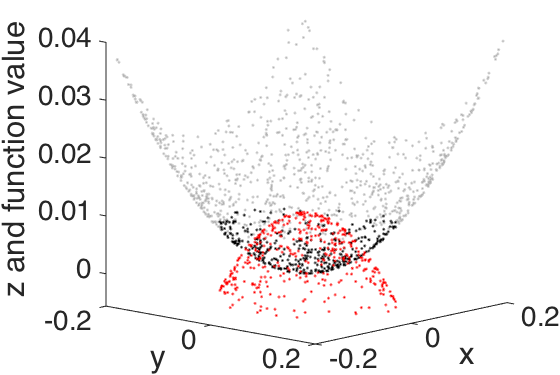
Finally, we take a look at the unit sphere S2S^{2} embedded in ℝ3\mathbb{R}^{3} with the center at (0,0,1)(0,0,1), and its corresponding kernel. We uniformly sample nn points, 𝒳={xi}i=1n⊂ℝ3\mathcal{X}=\{x_{i}\}_{i=1}^{n}\subset\mathbb{R}^{3}, from S2{S}^{2}. Fix n=10,000n=10,000 and run the LLE with 400400 nearest neighbors. See Figure 3 for the corresponding kernel. Note that the normalized kernel is not positive. These examples show that even with the simple manifolds, the corresponding kernels might be complicated.

Refer to caption
(a) S1S^{1} kernel
Refer to caption
(b) 𝕋1\mathbb{T}^{1} kernel
Refer to caption
(c) S2S^{2} kernel
Figure 3. 3(a): the sampled S1S^{1} is illustrated as the gray circle embedded in the (x,y)(x,y)-plane. The black thick line indicates the first 320320 neighbors of the central point x1000x_{1000}. The red line is the corresponding normalized kernel, KLLE​(x1000,y)∫KLLE​(x1000,y)​𝑑V​(y)\frac{K_{\texttt{LLE}}(x_{1000},y)}{\int K_{\texttt{LLE}}(x_{1000},y)dV(y)}, when K=80K=80, and the blue line is the corresponding normalized kernel when K=320K=320. It is clear that the kernel changes sign. 3(b): a surrogate of the sampled flat 11-dim torus 𝕋1\mathbb{T}^{1} is illustrated as the gray circle embedded in the (x,y)(x,y)-plane. The black thick line indicates the first 320320 neighbors of the central point x1000x_{1000}. The red line is the corresponding normalized kernel when K=80K=80, and the blue line is the corresponding normalized kernel when K=320K=320. In this flat manifold case, the kernel is constant. 3(c): a surrogate of the uniformly sampled 𝕊2\mathbb{S}^{2}. Only the first 10,00010,000 nearest points of the chosen x=(0,0,0)x=(0,0,0) are plotted as the gray points. Note that the scale of the xx and yy axes and the zz axis are different. The black points indicate the first 400400 neighbors of xx. The red points are the corresponding normalized kernel values when K=400K=400. It is clear that the kernel is non-positive.

4.3. Two-dimensional random tomography example

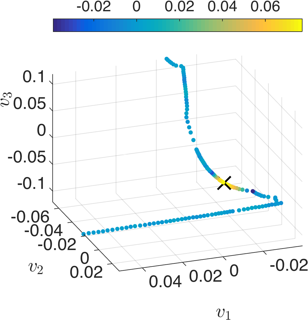
To further examine the capability of the LLE from the viewpoint of nonlinear dimension reduction, we consider the two-dimensional random tomography problem [26]. It is chosen because its geometrical structure is well known and complicated.

We briefly describe the dataset and refer the reader with interest to [26]. The classical two-dimensional transmission computerized tomography problem is to recover the function f:ℝ2→ℝf:\mathbb{R}^{2}\rightarrow\mathbb{R} from its Radon transform. In the parallel beam model, the Radon transform of ff is given by the line integral Rθ​f​(s)=∫x⋅θ=sf⁡(x)​𝑑xR_{\theta}f(s)=\int_{x\cdot\theta=s}f(x)dx, where θ∈S1\theta\in S^{1} is perpendicular to the beaming direction θ⟂∈S1\theta^{\perp}\in S^{1}, where S1S^{1} is the unit circle, and s∈ℝs\in\mathbb{R}. We call θ\theta the projection direction and Rθ​fR_{\theta}f the projected image. There are cases, however, in which we only have the projected images and the projection directions are unknown. In such cases, the problem at hand is to estimate ff from these projected images without knowing their corresponding projection directions. To better study this random projection problem, we need the following facts and assumptions. First, we know that for f∈L2​(ℝ2)f\in L^{2}(\mathbb{R}^{2}) with a compact support within B1​(0)B_{1}(0), the map R⋅​f:θ∈S1↦L2​([−1,1])R_{\cdot}f:\theta\in S^{1}\mapsto L^{2}([-1,1]) is continuous [26]. To simplify the discussion, we assume that there is no symmetry in ff; that is, Rθ1​fR_{\theta_{1}}f and Rθ2​fR_{\theta_{2}}f are different for all pairs of θ1≠θ2\theta_{1}\neq\theta_{2}. Next, take S:={si}i=1pS:=\{s_{i}\}_{i=1}^{p} to be the chosen set of sampling points on [−1,1][-1,1], where p∈ℕp\in\mathbb{N}. In this example, we assume that SS is a uniform grid on [−1,1][-1,1]; that is, si=−1+2​(i−1)/(p−1)s_{i}=-1+2(i-1)/(p-1). For θ∈S1\theta\in S^{1}, denote the discretization of the projection image Rθ​fR_{\theta}f as DS:L2​([−1,1])→ℝpD_{S}:L^{2}([-1,1])\to\mathbb{R}^{p}, which is defined by DS:Rθ​f↦(Rθ​f⋆hϵ​(s1),Rθ​f⋆hϵ​(s2),…,Rθ​f⋆hϵ​(sp))⊤∈ℝpD_{S}:R_{\theta}f\mapsto\left(R_{\theta}f\star h_{\epsilon}(s_{1}),R_{\theta}f\star h_{\epsilon}(s_{2}),\ldots,R_{\theta}f\star h_{\epsilon}(s_{p})\right)^{\top}\in\mathbb{R}^{p}, where hϵ​(x):=1ϵ​h​(xϵ)h_{\epsilon}(x):=\frac{1}{\epsilon}h(\frac{x}{\epsilon}), hh is a Schwartz function, hϵh_{\epsilon} converges weakly to the Dirac delta measure at 00 as ϵ→0\epsilon\to 0. Note that, in general, Rθ​fR_{\theta}f is a L2L^{2} function when ff is a L2L^{2} function. Therefore, we need a convolution to model the sampling step. We assume that the discretization DSD_{S} is dense enough, so that M1:={Dp∘Rθ​f}θ∈S1M^{1}:=\{D_{p}\circ R_{\theta}f\}_{\theta\in S^{1}} is also simple. In other words, we assume that pp is large enough so that M1M^{1} is a one-dimensional closed simple curved embedded in ℝp\mathbb{R}^{p} and M1M^{1} is diffeomorphic to S1S^{1}. Finally, we sample finite points from S1S^{1} uniformly and obtain the simulation.

With the above facts and assumptions, we sample the Radon transform 𝒳:={xi:=DS∘Rθif}i=1n⊂ℝp\mathcal{X}:=\{x_{i}:=D_{S}\circ R_{\theta_{i}}f\}_{i=1}^{n}\subset\mathbb{R}^{p} with finite projection directions {θi}i=1n\left\{\theta_{i}\right\}_{i=1}^{n}, where {θi}i=1n\left\{\theta_{i}\right\}_{i=1}^{n} is a finite uniform grid on S1S^{1}; that is, 𝒳\mathcal{X} is sampled from the one-dimensional manifold M1M^{1}. For the simulations with the Shepp-Logan phantom, we take n=4096n=4096, and the number of discretization points was p=128p=128. It has been shown in [26], that the DM could recover the M1M^{1} up to diffeomorphism, that is, we could achieve the nonlinear dimensional reduction. In order to avoid distractions, we do not consider any noise as is considered in [26], and focus our analysis on the clean dataset. The Shepp-Logan image, some examples of the projections and the results of PCA, DM and LLE, are shown in Figure 4. As is shown in [26], the PCA fails to embed 𝒳\mathcal{X} with only the first three principal components, while the DM succeeded. There can be additional discussion for the DM, particularly its robustness to the noise and metric design. They have been extensively discussed in [26], so they are not discussed here. For the LLE, we take ϵ=0.004\epsilon=0.004. The embedding results of the LLE with different regularization orders, ρ=8,3,−5\rho=8,3,-5, are shown. Due to the complicated geometrical structure, we encounter difficulty even to recover the topology of M1M^{1} by the LLE, if the regularization order is not chosen properly.

To examine whether the sign of the kernel corresponding to the LLE is indeterminate in this database, we fixed x3555∈𝒳x_{3555}\in\mathcal{X}, and apply the PCA to visualize its K=150K=150 neighbors. The kernel function is shown in Figure 4 as the color encoded on the embedded points. The sign of the kernel is indeterminate, as is predicted by the above theory due to the existence of curvature. In summary, we should be careful when we apply the LLE to a complicated real database.

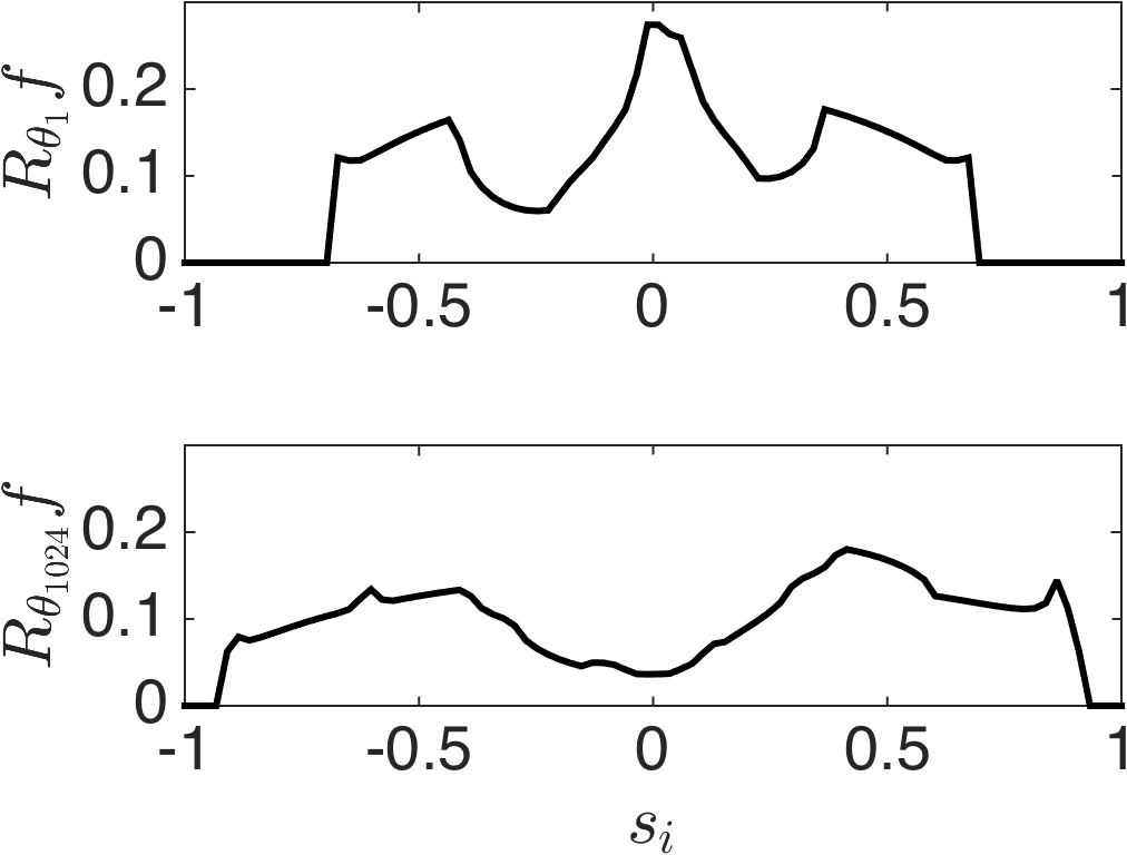
Refer to caption
Refer to caption
Refer to caption
Refer to caption
Refer to caption
Refer to caption
Refer to caption
Refer to caption
Refer to caption
Figure 4. Top row: the left panel is the Shepp-Logan phantom, the middle panel shows two projection images from two different projection directions, and the right panel shows the linear dimension reduction of the dataset by the first three principal components, u1,u2u_{1},u_{2} and u3u_{3}. Middle row: the left panel shows the diffusion map (DM) of the dataset, where the embedding is done by choosing the first two non-trivial eigenvectors of the graph Laplacian, ϕ2\phi_{2} and ϕ3\phi_{3}, and we simply take the Gaussian kernel to design the affinity without applying the α\alpha-normalization technique [10], the middle panel shows the DM of the dataset, where we apply the α\alpha-normalization technique when α=1\alpha=1, and the right panel shows that the sign of the kernel corresponding to the locally linear embedding (LLE) is indeterminate, where the black cross indicates x3555x_{3555}, and the kernel value on its neighbors are encoded by color (the neighbors are visualized by the top three principal components, v1v_{1}, v2v_{2}, and v3v_{3}). Bottom row: the embedding using the second and third eigenvectors of the LLE, ψ2\psi_{2} and ψ3\psi_{3}, under different setups are shown. The left panel shows the result with ρ=−5\rho=-5, the middle panel shows the result with ρ=3\rho=3, and the right panel shows the result with ρ=8\rho=8. The results shows the importance of choosing the regularization and are explained by the theory.

5. ϵ\epsilon-radius neighborhood v.s. KK nearest neighborhood

In the original article [23], the KNN scheme was proposed for the LLE algorithm. However, the analysis in this paper has been based on the ϵ\epsilon-radius neighborhood scheme. These two schemes are closely related asymptotically from the viewpoint of density function estimation [22]. The following argument shows that the developed theorems are actually transferrable to the KNN scheme under the manifold setup.

We follow the notations in Section 3.1. For ι⁡(xk)∈𝒳\iota(x_{k})\in\mathcal{X}, take KK nearest neighbors of ι⁡(xk)\iota(x_{k}), namely ι⁡(xk,1),…,ι⁡(xk,K)\iota(x_{k,1}),\ldots,\iota(x_{k,K}), with respect to the Euclidean distance. Intuitively, KK is closely related to the volume of the minimal ball centered at xkx_{k} with the radius ϵ⁡(xk)\epsilon(x_{k}) containing the KK nearest neighbors of xkx_{k}, where ϵ⁡(xk){\epsilon(x_{k})} depends on KK and the p.d.f.; that is, we expect to have

n​P​(xk)​vol​(Dxk)≈K,nP(x_{k})\text{vol}(D_{x_{k}})\approx K\,, (5.1)

where Dx:=Bϵ⁡(x)ℝp​(ι⁡(x))∩ι⁡(M)D_{x}:=B^{\mathbb{R}^{p}}_{{\epsilon(x)}}(\iota(x))\cap\iota(M) is the minimal ball centered at x∈Mx\in M with the radius ϵ⁡(x)>0\epsilon(x)>0 so that DxD_{x} contains the KK nearest neighbors of xx. Under the smoothness assumption of the p.d.f. and the manifold setup, we claim that asymptotically when n→∞n\to\infty, this relationship holds uniformly over the manifold a.s., if K=K⁡(n)K=K(n), K/log⁡(n)→∞K/\log(n)\to\infty and K/n→0K/n\to 0 as n→∞n\to\infty. This claim could be achieved by slightly modifying the argument for the Theorem in [11] to obtain the large deviation bound for (5.1) when nn is finite. To bound Pr{supx∈M|Kn​vol​(Dx)−P(x)|>α}\text{Pr}\{\sup_{x\in M}|\frac{K}{n\text{vol}(D_{x})}-P(x)|>\alpha\}, where α>0\alpha>0, it is sufficient to bound the two terms on the right hand side of [11, equation (10)]. By a straightforward calculation of the equations on page 539 in [11], we achieve the bound Pr{supx∈M|Kn​vol​(Dx)−P(x)|>α}≤poly(n)e−c​K​α3\text{Pr}\{\sup_{x\in M}|\frac{K}{n\text{vol}(D_{x})}-P(x)|>\alpha\}\leq\text{poly}(n)e^{-cK\alpha^{3}}, where cc is a constant depending on dd and the upper bounds of P⁡(x)P(x) on MM, and poly​(n)=3​(1+2p+3​np+3)\text{poly}(n)=3(1+2^{p+3}n^{p+3}).33 3 This can be observed by combining [11, equations (6) (7) (9) and (10)]. The second term on the right hand side of [11, equation (10)] is dominated by the first term. To bound the first term, we can substitute δ=K​β4​n​(PM+β)\delta=\frac{K\beta}{4n(P_{M}+\beta)} and M=4​k​PMn​βM=\frac{4kP_{M}}{n\beta} into the fourth unlabeled equation on page 539 in [11], where PMP_{M} is the upper bound of p.d.f. In the fourth unlabeled equation, α\alpha is the upper bound of the volume ratio of B2​ϵ​(x)ℝp​(ι⁡(x))∩ι⁡(M)B^{\mathbb{R}^{p}}_{2\epsilon(x)}(\iota(x))\cap\iota(M) and Bϵ⁡(x)ℝp​(ι⁡(x))∩ι⁡(M)B^{\mathbb{R}^{p}}_{\epsilon(x)}(\iota(x))\cap\iota(M), which can be chosen as 3d3^{d} when ϵ⁡(x)\epsilon(x) is sufficiently small. Finally, we use the fact that when β\beta is small, the equation follows. Therefore, if we choose α=(2​p+10c)1/3​(log⁡nK)1/3\alpha=(\frac{2p+10}{c})^{1/3}(\frac{\log n}{K})^{1/3}, with probability greater than 1−n−21-n^{-2}, we have uniformly Kn​vol​(Dx)=P⁡(x)+O⁡(α)\frac{K}{n\text{vol}(D_{x})}=P(x)+O(\alpha). Note that by the assumption, α→0\alpha\to 0 as n→∞n\to\infty. We conclude that with probability greater than 1−n−21-n^{-2},

ϵ⁡(x)=(d|Sd−1|)1/d​(Kn​P​(x))1/d​(1+O⁡((log⁡nK)1/3)),\epsilon(x)=\Big(\frac{d}{|S^{d-1}|}\Big)^{1/d}\Big(\frac{K}{nP(x)}\Big)^{1/d}\Big(1+O\Big(\Big(\frac{\log n}{K}\Big)^{1/3}\Big)\Big)\,, (5.2)

where we use the fact that vol​(Dx)=|Sd−1|d​ϵ​(x)d+O⁡(ϵ​(x)d+1)\text{vol}(D_{x})=\frac{|S^{d-1}|}{d}\epsilon(x)^{d}+O(\epsilon(x)^{d+1}) when ϵ⁡(x)\epsilon(x) is sufficiently small. It is transparent that ϵ⁡(x)\epsilon(x) depends on nn and ϵ⁡(x)→0\epsilon(x)\to 0 a.s. as n→∞n\to\infty since K⁡(n)/n→0K(n)/n\to 0 by assumption. In other words, ϵ\epsilon is not a constant value. It is a function depending on the p.d.f.. If we requre K=K⁡(n)K=K(n) to additionally satisfy K⁡(n)n​K​(n)d/2log⁡(n)d/2→∞\frac{K(n)}{n}\frac{K(n)^{d/2}}{\log(n)^{d/2}}\to\infty, then ϵ⁡(xk)\epsilon(x_{k}) satisfies nn1/2​ϵ​(x)d/2+1→0\frac{\sqrt{n}}{n^{1/2}\epsilon(x)^{d/2+1}}\to 0 a.s.. On the other hand, notice that the statement of Theorem 3.3 is pointwise. Therefore, its proof could be directly employed to the case when ϵ\epsilon is chosen pointwisely, and hence the KNN scheme. As a result, if we take ρ=3\rho=3 and is K/n→0K/n\to 0, K/log⁡(n)→∞K/\log(n)\to\infty, and (K/n)​(K/log⁡(n))d/2→∞(K/n)(K/\log(n))^{d/2}\to\infty when n→∞n\to\infty, by plugging (5.2) into Theorem 3.3, when nn is sufficiently large, the following convergence holds for all xkx_{k} with probability greater than 1−2​n−21-2n^{-2}:

∑j=1Kwk​(j)​f​(xk,j)\displaystyle\sum_{j=1}^{K}w_{k}(j)f(x_{k,j}) −f⁡(xk)=(d|Sd−1|)1/d2​(d+2)​Δ​f​(xk)P​(xk)2/d​(Kn)2/d\displaystyle-f(x_{k})=\frac{(\frac{d}{|S^{d-1}|})^{1/d}}{2(d+2)}\frac{\Delta f(x_{k})}{P(x_{k})^{2/d}}\Big(\frac{K}{n}\Big)^{2/d}
+O⁡((log⁡(n)K)1/3​(Kn)2/d)+O⁡((log⁡(n)K)1/2​(Kn)1/d).\displaystyle+O\Big(\Big(\frac{\log(n)}{K}\Big)^{1/3}\Big(\frac{K}{n}\Big)^{2/d}\Big)+O\Big(\Big(\frac{\log(n)}{K}\Big)^{1/2}\Big(\frac{K}{n}\Big)^{1/d}\Big)\,. (5.3)

In summary, unless the sampling is uniform, we do not obtain the Laplace-Beltrami operator with the KNN scheme. Based on the expansion (5.3), to obtain the Laplace-Beltrami operator with the KNN scheme, we could numerically consider a “normalized LLE matrix”; that is, find the eigen-structure of L~:=ℰ−1​(W−I)\tilde{L}:=\mathcal{E}^{-1}(W-I), where WW is the ordinary LLE matrix, and ℰ∈ℝn×n\mathcal{E}\in\mathbb{R}^{n\times n} is a diagonal matrix so that ℰi​i=ϵ​(xi)2\mathcal{E}_{ii}=\epsilon(x_{i})^{2}. Since the analysis of the pointwise convergence of L~\tilde{L} is similar to that of Theorem 3.3, we skip the details here.

6. Relationship with two statistical topics

6.1. Locally linear regression

Based on the above theoretical study under the manifold setup, we could link the LLE to the locally linear regression (LLR) [16, 9]. Recall that in the LLR, we locally fit a linear function to the response, and the associated kernel depends on the inverse of a variation of the covariance matrix. We summarize how the LLR is operated. Consider the following regression model

Y=m⁡(X)+σ⁡(X)​ξ,Y=m(X)+\sigma(X)\,\xi, (6.1)

where ξ\xi is a random error independent of XX with 𝔼⁡(ξ)=0\mathbb{E}(\xi)=0 and Var⁡(ξ)=1\operatorname{Var}(\xi)=1, and both the regression function mm and the conditional variance function σ2\sigma^{2} are defined on ℝd\mathbb{R}^{d}. Let {(Xl,Yl)}l=1n\{(X_{l},Y_{l})\}_{l=1}^{n} denote a random sample observed from model (6.1) with 𝒳:={Xl}l=1n\mathcal{X}:=\{X_{l}\}_{l=1}^{n} being sampled from XX. Given {(Xl,Yl)}l=1n\{(X_{l},Y_{l})\}_{l=1}^{n} and x∈ℝdx\in\mathbb{R}^{d}, the problem is then to estimate m⁡(x)m({x}) assuming enough smoothness of mm. Choose a smooth kernel function with fast decay K:[0,∞]→ℝK:[0,\infty]\to\mathbb{R} and a bandwidth ϵ>0\epsilon>0. The LLR estimator for m⁡(x)m(x) is defined as e1⊤​𝜷^xe_{1}^{\top}\hat{\bm{\beta}}_{x}, where

𝜷^x\displaystyle\hat{\bm{\beta}}_{x} =arg⁡min𝜷∈ℝd+1​(𝐘−𝐗x​𝜷)⊤​𝐖x​(𝐘−𝐗x​𝜷),\displaystyle=\arg\min_{\bm{\beta}\in\mathbb{R}^{d+1}}(\mathbf{Y}-\mathbf{X}_{x}\bm{\beta})^{\top}\mathbf{W}_{x}(\mathbf{Y}-\mathbf{X}_{x}\bm{\beta})\,, (6.2)
𝐘\displaystyle\mathbf{Y} =(Y1,…,Yn)⊤,𝐗x=[1…1X1…Xn]⊤∈ℝn×(d+1),\displaystyle=\left(Y_{1},\ldots,Y_{n}\right)^{\top},\quad\mathbf{X}_{x}=\bigg[\begin{array}[]{ccc}1&\dots&1\\ X_{1}&\dots&X_{n}\\ \end{array}\bigg]^{\top}\in\mathbb{R}^{n\times(d+1)},
𝐖x\displaystyle\mathbf{W}_{x} =diag​(Kϵ​(X1,x),…,Kϵ​(Xn,x))∈ℝn×n,\displaystyle=\texttt{diag}\left(K_{\epsilon}(X_{1},x),\ldots,K_{\epsilon}(X_{n},x)\right)\in\mathbb{R}^{n\times n},

and Kϵ​(Xl,x):=ϵ−d​K​(‖Xl−x‖ℝd/ϵ)K_{\epsilon}(X_{l},x):=\epsilon^{-d}K\big(\|X_{l}-x\|_{\mathbb{R}^{d}}\big/\epsilon\big). By a direct expansion, (6.2) becomes

𝜷^x=(𝐗x⊤​𝐖x​𝐗x)−1​𝐗x⊤​𝐖x​𝐘\hat{\bm{\beta}}_{x}=(\mathbf{X}_{x}^{\top}\mathbf{W}_{x}\mathbf{X}_{x})^{-1}\mathbf{X}^{\top}_{x}\mathbf{W}_{x}\mathbf{Y} (6.5)

if (𝐗x⊤​𝐖x​𝐗x)−1(\mathbf{X}^{\top}_{x}\mathbf{W}_{x}\mathbf{X}_{x})^{-1} exists. We have 𝐗x=[𝟏n⊤𝐆x]\mathbf{X}_{x}=\begin{bmatrix}\bm{1}_{n}^{\top}\\ \mathbf{G}_{x}\end{bmatrix}, where 𝐆x\mathbf{G}_{x} is the data matrix associated with {Xi}i=1n\{X_{i}\}_{i=1}^{n} centered at xx. By yet another direct expansion by the block inversion,

e1⊤​𝜷^x=wx(LLR)⊤​𝐘,e_{1}^{\top}\hat{\bm{\beta}}_{x}={w^{(\texttt{LLR})}_{x}}^{\top}\mathbf{Y}\,, (6.6)

where wx(LLR)w^{(\texttt{LLR})}_{x} is called the “smoothing kernel” and satisfies

wx(LLR):=𝟏n⊤​𝐖x−𝟏n⊤​𝐖x​𝐆x⊤​(𝐆x​𝐖x​𝐆x⊤)−1​𝐆x​𝐖x𝟏n⊤​𝐖x​𝟏n−𝟏n⊤​𝐖x​𝐆x⊤​(𝐆x​𝐖x​𝐆x⊤)−1​𝐆x​𝐖x​𝟏n.w^{(\texttt{LLR})}_{x}:=\frac{\bm{1}_{n}^{\top}\mathbf{W}_{x}-\bm{1}_{n}^{\top}\mathbf{W}_{x}\mathbf{G}^{\top}_{x}(\mathbf{G}_{x}\mathbf{W}_{x}\mathbf{G}_{x}^{\top})^{-1}\mathbf{G}_{x}\mathbf{W}_{x}}{\bm{1}_{n}^{\top}\mathbf{W}_{x}\bm{1}_{n}-\bm{1}_{n}^{\top}\mathbf{W}_{x}\mathbf{G}^{\top}_{x}(\mathbf{G}_{x}\mathbf{W}_{x}\mathbf{G}_{x}^{\top})^{-1}\mathbf{G}_{x}\mathbf{W}_{x}\bm{1}_{n}}. (6.7)

Through a direct comparison, we see that the vector wx(LLR)w^{(\texttt{LLR})}_{x} is almost the same as the weight matrix in the LLE algorithm shown in (2.17), except the weighting by the chosen kernel – in the LLE, the kernel function and its support are both determined by the data, while in the LLR the kernel is selected in the beginning and the data points are weighted by the chosen kernel like 𝐆x​𝐖x\mathbf{G}_{x}\mathbf{W}_{x}. If we choose the kernel to be a zero-one kernel with the support on the ball centered at xx with the radius ϵ\epsilon, then we “recover” (2.17).

Under the low dimensional manifold setup, 𝐆x​𝐖x​𝐆x⊤\mathbf{G}_{x}\mathbf{W}_{x}\mathbf{G}_{x}^{\top} might not be of full rank. Note that the term 𝐆x​𝐖x​𝐆x⊤\mathbf{G}_{x}\mathbf{W}_{x}\mathbf{G}_{x}^{\top} is the weighted local covariance matrix, which is considered in [25] to estimate the tangent space. Unlike the regularized pseudo-inverse (2.15) in the LLE, to handle this degeneracy issue, in LLR the data matrix 𝐆x\mathbf{G}_{x} is constructed by projecting the point cloud to the estimated tangent plane. This projection step could be understood as taking the Moore-Penrose pseudo-inverse approach to handle the degeneracy. We mention that in [9, Section 6], the relationship between the LLR and the manifold learning under the manifold setup is established. It is shown that asymptotically, the smooth matrix from the kernel wx(LLR)w^{(\texttt{LLR})}_{x} leads to the Laplace-Beltrami operator. The result is parallel to the reported result in this paper.

These relationships between the LLE and the LLR suggest the possibility of fitting the data locally by taking the locally polynomial regression into account, and generalizing the barycentric coordinate by fitting a polynomial function locally. This might lead to a variation of the LLE that catches more delicate structure of the manifold, in a different adaptive way. Since this direction is outside the scope of this paper, the study of this possibility is left to future studies.

6.2. Error in variable

In this work, we analyze the LLE under the assumption that the dataset is randomly sampled directly from a manifold, without any influence of the noise. However, the noise is inevitable and a further study is needed. By the analysis, we observe that the LLE takes care of the error in variable challenge “in some sense”.

Suppose the dataset is {yi}i=1n⊂ℝp\{y_{i}\}_{i=1}^{n}\subset\mathbb{R}^{p}, where yi=zi+ξiy_{i}=z_{i}+\xi_{i}, ziz_{i} is supported on a manifold and ξi\xi_{i} is an i.i.d. noise with good properties. The question is to ask how much information the LLE could recover from {zi}i=1n\{z_{i}\}_{i=1}^{n}. A parallel problem for the GL, or the more general graph connection Laplacian (GCL), has been studied in [14, 15]. It shows that the spectral properties of the GL and GCL are robust to noise. For the LLE, while a similar analysis could be applied, if we view the LLE as a kernel method and show a similar result, we mention that we might benefit by taking the special algorithmic structure of the LLE into account.

When the dimension of the dataset is high, the noise might have a nontrivial behavior. For example, when the dimension of the database p=p⁡(n)p=p(n) satisfies p⁡(n)/n→γ>0p(n)/n\to\gamma>0 when n→∞n\to\infty (known as the large pp and large nn setup), it is problematic to even estimate the covariance matrix. Note that the covariance matrix is directly related to the LLE algorithm since the covariance matrix appears in the regularized pseudo inverse, ℐn​ϵd+ρ​(G¯n​G¯n⊤)\mathcal{I}_{n\epsilon^{d+\rho}}(\bar{G}_{n}\bar{G}_{n}^{\top}), where G¯n\bar{G}_{n} is the local data matrix associated with yky_{k} determined from the noisy database {yi}i=1n\{y_{i}\}_{i=1}^{n}, and G¯n​G¯n⊤\bar{G}_{n}\bar{G}_{n}^{\top} is the covariance matrix. Under the large pp and large nn setup, the eigenvalues and eigenvectors of the covariance matrix will both be biased, depending on the “signal-to-noise ratio” and γ\gamma [21]. A careful manipulation of the noise, or a modification of the covariance matrix estimator, is needed in order to address these introduced biases. For example, the “shrinkage technique” was introduced to correct the eigenvalue bias with a theoretical guarantee [26, 12]. The covariance matrix estimator based on the shrinkage technique is C~n:=∑l=1pf⁡(λl)​ul​ul⊤\tilde{C}_{n}:=\sum_{l=1}^{p}f(\lambda_{l})u_{l}u_{l}^{\top}, where ulu_{l} and λl\lambda_{l} form the ll-th eigenpair of G¯n​G¯n⊤\bar{G}_{n}\bar{G}_{n}^{\top} and ff is the designed shrinkage function.

A direct comparison shows that the regularized pseudo inverse in the LLE behaves like a shrinkage technique. Recall that ℐn​ϵd+ρ​(G¯n​G¯n⊤)=∑l=1rn1λl+n​ϵd+ρ​ul​ul⊤\mathcal{I}_{n\epsilon^{d+\rho}}(\bar{G}_{n}\bar{G}_{n}^{\top})=\sum_{l=1}^{r_{n}}\frac{1}{\lambda_{l}+n\epsilon^{d+\rho}}u_{l}u_{l}^{\top} (2.15), where rnr_{n} is the rank of G¯n​G¯n⊤\bar{G}_{n}\bar{G}_{n}^{\top}, the shrinkage function is f⁡(x)=1x+n​ϵd+ρ​χ(0,∞)​(x)f(x)=\frac{1}{x+n\epsilon^{d+\rho}}\chi_{(0,\infty)}(x), and χ\chi is the indicator function. Although how ff corrects the noise impact is outside the scope of this paper, it would be potential to carefully improve the regularized pseudo inverse by taking the shrinkage technique into account. In other words, by modifying the barycentric coordinate evaluation and applying the technique discussed in [14, 15], it is possible to improve the LLE algorithm. An extensive study of the topic will be reported in the upcoming research.

7. Conclusions and Discussion

We provide an asymptotical analysis of the LLE under the manifold setup. The theoretical results indicate that asymptotically, the LLE generally may not give the expected Laplace-Beltrami operator, unless the regularization is chosen properly. From the integral operator viewpoint, the corresponding kernel of the LLE in general is not positive. Therefore, the LLE in general is not a diffusion operator. Some direct calculations of the LLE operator over simple manifolds, like the sphere, indicate that asymptotically the fourth order differential operator might pop out as the dominant term, if the regularization is chosen to be too small. The numerical results support the theoretical findings. In addition, we also discuss the relationship between the LLE and two statistical problems, the LLR and the error in variable problem, and point out the potential future work.

There are more important topics we do not explore in this paper. First, note that the pointwise convergence result established in this paper comes from a careful analysis of the “fit locally” part of the LLE algorithm. However, it is not sufficient to fully understand the “think globally” part of the LLE algorithm. Recall that we evaluate the eigen-decomposition of the LLE matrix for the embedding in the last step of the LLE algorithm. The theoretical and numerical results suggest that the eigen-structure of the LLE matrix provides an approximation of the eigen-structure of the Laplace-Beltrami operator. The embedding in the last step could therefore be understood from the point of view of the spectral embedding theory [6, 7]. The eigen-structure of the LLE matrix integrates the local information. As a result, we catch the “think globally” part. However, the pointwise convergence is not strong enough to guarantee the spectral convergence. In other words, we need to show that asymptotically, the eigen-decomposition provides a proper approximation of the eigen-structure of the Laplace-Beltrami operator. While a similar proof of that in [27] could be slightly modified to achieve the spectral convergence of the LLE, however, more may be needed, such as the spectral convergence rate, from the statistical viewpoint. Recently, there have been some relevant works for the GL under the manifold model in this direction [18, 34]. Based on the special structure of the LLE, like the regularization, the optimal convergence rate of the LLE could be different and additional exploration is needed. The result will be reported in the future work.

Another important topic is the appearance of the fourth order differential operator in the LLE, when the manifold has a special structure and the regularization is improperly chosen. Although it would be a by-product, it would be interesting to ask if it is possible to take the fourth order differential operator into account in the data analysis and which kind of information could be extracted from the dataset. It would also be interesting to ask if it is possible to directly obtain the fourth order differential operator for more general manifolds with a slight modification of the LLE algorithm. A direct benefit of this possibility is linked back to the regression problem, such as the LLR. If we could directly eliminate the second order term, the regression result could be more accurate. We leave this study direction to the future work.

Acknowledgement

Hau-tieng Wu’s research is partially supported by Sloan Research Fellow FR-2015-65363. He acknowledges the continuous support from the Department of Mathematics, University of Toronto.

References

  • [1] A. L. Andrew and R. C. E. Tan. Computation of derivatives of repeated eigenvalues and the corresponding eigenvectors of symmetric matrix pencils. SIAM Journal on Matrix Analysis and Applications, 20(1):78–100, 1998.
  • [2] H. Baumgärtel. Analytic perturbation theory for matrices and operators. Operator theory. Birkhäuser Verlag, 1985.
  • [3] M. Belkin and P. Niyogi. Laplacian Eigenmaps for Dimensionality Reduction and Data Representation. Neural. Comput., 15(6):1373–1396, 2003.
  • [4] M. Belkin and P. Niyogi. Towards a theoretical foundation for Laplacian-based manifold methods. In Proceedings of the 18th Conference on Learning Theory (COLT), pages 486–500, 2005.
  • [5] M. Belkin and P. Niyogi. Convergence of Laplacian eigenmaps. In Adv. Neur. In.: Proceedings of the 2006 Conference, volume 19, page 129. The MIT Press, 2007.
  • [6] P. Bérard. Spectral Geometry: Direct and Inverse Problems. Springer, 1986.
  • [7] P. Bérard, G. Besson, and S. Gallot. Embedding Riemannian manifolds by their heat kernel. Geom. Funct. Anal., 4:373–398, 1994.
  • [8] Jeff Cheeger, Mikhail Gromov, Michael Taylor, et al. Finite propagation speed, kernel estimates for functions of the laplace operator, and the geometry of complete riemannian manifolds. Journal of Differential Geometry, 17(1):15–53, 1982.
  • [9] M.-Y. Cheng and H.-T. Wu. Local linear regression on manifolds and its geometric interpretation. J. Am. Stat. Assoc., 108:1421–1434, 2013.
  • [10] R. R. Coifman and S. Lafon. Diffusion maps. Appl. Comput. Harmon. Anal., 21(1):5–30, 2006.
  • [11] L. P. Devroye and T. J. Wagner. The strong uniform consistency of nearest neighbor density estimates. Ann. Stat., 5(3):536–540, 1977.
  • [12] D. L. Donoho, M. Gavish, and I. M. Johnstone. Optimal Shrinkage of Eigenvalues in the Spiked Covariance Model. ArXiv e-prints, 2013.
  • [13] D. L. Donoho and C. Grimes. Hessian eigenmaps: Locally linear embedding techniques for high-dimensional data. P. Natl. Acad. Sci. USA, 100(10):5591–5596, 2003.
  • [14] N. El Karoui. On information plus noise kernel random matrices. Ann. Stat., 38(5):3191–3216, 2010.
  • [15] N. El Karoui and H.-T. Wu. Connection graph Laplacian methods can be made robust to noise. Ann. Stat., 44(1):346–372, 2016.
  • [16] J. Fan and I. Gijbels. Local Polynomial Modelling and Its Applications. Chapman and Hall/CRC, 1996.
  • [17] T. Gao. The Diffusion Geometry of Fibre Bundles. ArXiv e-prints, 2016.
  • [18] N. Garcia Trillos and D. Slepcev. A variational approach to the consistency of spectral clustering. Appl. Comput. Harmon. Anal., pages 1–39, 2015.
  • [19] E. Giné and V. Koltchinskii. Empirical graph laplacian approximation of laplace-beltrami operators: Large sample results. In Anthony Bonato and Jeannette Janssen, editors, IMS Lecture Notes, volume 51 of Monograph Series, pages 238–259. The Institute of Mathematical Statistics, 2006.
  • [20] M. Hein, J. Audibert, and U. von Luxburg. From graphs to manifolds - weak and strong pointwise consistency of graph Laplacians. In Proceedings of the 18th Conference on Learning Theory (COLT), pages 470–485, 2005.
  • [21] I. M. Johnstone. High dimensional statistical inference and random matrices. arXiv:math/0611589v1, 2006.
  • [22] D. S. Moore and J. W. Yackel. Consistency Properties of Nearest Neighbor Density Function Estimators. Ann. Statist., 5(1):143–154, 1977.
  • [23] S. T. Roweis and L. K. Saul. Nonlinear dimensionality reduction by locally linear embedding. Science, 290(5500):2323–2326, 2000.
  • [24] A. Singer. From graph to manifold Laplacian: The convergence rate. Appl. Comput. Harmon. Anal., 21(1):128–134, 2006.
  • [25] A. Singer and H.-T. Wu. Vector diffusion maps and the connection Laplacian. Comm. Pure Appl. Math., 65(8):1067–1144, 2012.
  • [26] A. Singer and H.-T. Wu. 2-d tomography from noisy projections taken at unknown random directions. SIAM J. Imaging Sci., 6(1):136–175, 2013.
  • [27] A. Singer and H.-T. Wu. Spectral convergence of the connection laplacian from random samples. Information and Inference: A Journal of the IMA, 6(1):58–123, 2017.
  • [28] O. Smolyanov, H.v. Weizsacker, and O. Wittich. Chernoff’s theorem and discrete time approximations of brownian motion on manifolds. Potential Anal., 26(1):1–29, 2007.
  • [29] Elias M Stein and Guido Weiss. Introduction to Fourier analysis on Euclidean spaces (PMS-32), volume 32. Princeton university press, 2016.
  • [30] J. B. Tenenbaum, V. de Silva, and J. C. Langford. A Global Geometric Framework for Nonlinear Dimensionality Reduction. Science, 290(5500):2319–2323, 2000.
  • [31] N.P. Van Der Aa, H.G. Ter Morsche, and R.R.M. Mattheij. Computation of eigenvalue and eigenvector derivatives for a general complex-valued eigensystem. Electronic Journal of Linear Algebra, 16(1):300–314, 2007.
  • [32] L. van der Maaten and G. Hinton. Visualizing Data using t-SNE. Journal of Machine Learning Research, 9:2579–2605, 2008.
  • [33] U. von Luxburg, M. Belkin, and O. Bousquet. Consistency of spectral clustering. Ann. Stat., 36(2):555–586, April 2008.
  • [34] X. Wang. Spectral Convergence Rate of Graph Laplacian. ArXiv e-prints, 1510.08110, 2015.
  • [35] K.Q. Weinberger and L.K. Saul. An introduction to nonlinear dimensionality reduction by maximum variance unfolding. Aaai, pages 1683–1686, 2006.
  • [36] Z. Zhang and J. Wang. Mlle: Modified locally linear embedding using multiple weights. Advances in neural information processing systems, pages 1593–1600, 2006.
  • [37] Z. Zhang and H. Zha. Principal manifolds and nonlinear dimensionality reduction via tangent space alignment. SIAM J. Sci. Comput., 26:313 – 338, 2004.

Online Supplementary Information for
Think globally, fit locally under the Manifold Setup
Asymptotic Analysis of Locally Linear Embedding
by Hau-Tieng Wu and Nan Wu

Appendix A Perturbation analysis of eigenvalue and eigenvectors

Suppose A:ℝ→S⁡(p)A:\mathbb{R}\rightarrow S(p), where S⁡(p)S(p) is the set of real symmetric p×pp\times p matrices, is an analytic function around 00. In this appendix, we are going to introduce an algorithm to calculate the eigenvalues and orthonormal eigenvectors of A⁡(ϵ)A(\epsilon) when ϵ\epsilon is small enough. The method introduced in this appendix follows the standard approach, like [1, 31]. For discussion of more general matrices, interested readers are referred to [31].

Suppose

A⁡(0)=[λ​Id×d000],A(0)=\begin{bmatrix}\lambda I_{d\times d}&0\\ 0&0\\ \end{bmatrix},

where 0<d<p0<d<p and λ≠0\lambda\neq 0. Decompose A⁡(0)A(0) by

A⁡(0)​X​(0)=X⁡(0)​Λ​(0),A(0)X(0)=X(0)\Lambda(0), (A.1)

where Λ⁡(0)=A⁡(0)\Lambda(0)=A(0) is a diagonal matrix consisting of eigenvalues of A⁡(0)A(0), and

X⁡(0)=[X100X2]∈O⁡(p),X(0)=\begin{bmatrix}X_{1}&0\\ 0&X_{2}\\ \end{bmatrix}\in O(p),

where X1∈O⁡(d)X_{1}\in O(d) and X2∈O⁡(p−d)X_{2}\in O(p-d). Note that due to the possible nontrivial multiplicity of eigenvalues, X⁡(0)X(0) may not be uniquely determined. Take the Taylor expansion of AA around 00 as

A⁡(ϵ)=A⁡(0)+A′​(0)​ϵ+12​A′′​(0)​ϵ2+O⁡(ϵ3),A(\epsilon)=A(0)+A^{\prime}(0)\epsilon+\frac{1}{2}A^{\prime\prime}(0)\epsilon^{2}+O(\epsilon^{3})\,,

where ϵ>0\epsilon>0 is sufficiently small, A′​(0)A^{\prime}(0) and A′′​(0)A^{\prime\prime}(0) are divided into blocks of the same size as those of A⁡(0)A(0) by

A′​(0)=[A11′A12′A21′A22′],A′′​(0)=[A11′′A12′′A21′′A22′′],A^{\prime}(0)=\begin{bmatrix}A^{\prime}_{11}&A^{\prime}_{12}\\ A^{\prime}_{21}&A^{\prime}_{22}\\ \end{bmatrix},\quad A^{\prime\prime}(0)=\begin{bmatrix}A^{\prime\prime}_{11}&A^{\prime\prime}_{12}\\ A^{\prime\prime}_{21}&A^{\prime\prime}_{22}\\ \end{bmatrix},

where A11′∈S⁡(d)A^{\prime}_{11}\in S(d), A22′∈S⁡(p−d)A^{\prime}_{22}\in S(p-d), A11′′∈S⁡(d)A^{\prime\prime}_{11}\in S(d) and A22′′∈S⁡(p−d)A^{\prime\prime}_{22}\in S(p-d). Let Λ⁡(ϵ)∈ℝp×p\Lambda(\epsilon)\in\mathbb{R}^{p\times p} be the diagonal matrix consisting of eigenvalues of A⁡(ϵ)A(\epsilon) and X⁡(ϵ)∈ℝp×pX(\epsilon)\in\mathbb{R}^{p\times p} be the matrix formed by the corresponding eigenvectors, i.e.

A⁡(ϵ)​X​(ϵ)=X⁡(ϵ)​Λ​(ϵ).A(\epsilon)X(\epsilon)=X(\epsilon)\Lambda(\epsilon)\,. (A.2)

Since AA is symmetric, XX and Λ\Lambda are both analytic around 00 based on [2, Section 3.6.2, Theorem 1]. We thus have the following Taylor expansion when ϵ\epsilon is sufficiently small:

Λ⁡(ϵ)=Λ⁡(0)+ϵ​Λ′​(0)+12​ϵ2​Λ′′​(0)+O⁡(ϵ3),\Lambda(\epsilon)=\Lambda(0)+\epsilon\Lambda^{\prime}(0)+\frac{1}{2}\epsilon^{2}\Lambda^{\prime\prime}(0)+O(\epsilon^{3}),
X⁡(ϵ)=X⁡(0)+X′​(0)​ϵ+O⁡(ϵ2).X(\epsilon)=X(0)+X^{\prime}(0)\epsilon+O(\epsilon^{2}).

Here Λ⁡(0)\Lambda(0), Λ′​(0)\Lambda^{\prime}(0) and Λ′′​(0)\Lambda^{\prime\prime}(0) are all diagonal matrices and columns of X⁡(ϵ)X(\epsilon) form an orthogonal set. Note that if we normalize X⁡(ϵ)X(\epsilon) to be in O⁡(p)O(p), then by the fact that the Lie algebra of O⁡(p)O(p) is the set of anti-symmetric matrices, we know that X​(0)−1​X′​(0)X(0)^{-1}X^{\prime}(0) is an anti-symmetric matrix. We discuss the eigendecomposition of A⁡(ϵ)A(\epsilon) under two different setups, depending on the multiplicity of eigenvalues.

When there is no repeated eigenvalue in both A11′A^{\prime}_{11} and A22′A^{\prime}_{22}. In the first case, we assume that the eigenvalues of A11′A^{\prime}_{11} are distinct and the eigenvalues of A22′A^{\prime}_{22} are distinct (but the eigenvalues of A11′A^{\prime}_{11} and the eigenvalues of A22′A^{\prime}_{22} could overlap). To get Λ⁡(ϵ)\Lambda(\epsilon) up to the first order, we need to solve Λ′​(0)\Lambda^{\prime}(0). To determined Λ′​(0)\Lambda^{\prime}(0), we check the first order derivative of A⁡(ϵ)A(\epsilon) at ϵ=0\epsilon=0. Differentiate (A.2) and we get

A′​(0)​X​(0)+A⁡(0)​X′​(0)=X′​(0)​Λ​(0)+X⁡(0)​Λ′​(0).A^{\prime}(0)X(0)+A(0)X^{\prime}(0)=X^{\prime}(0)\Lambda(0)+X(0)\Lambda^{\prime}(0)\,.

Denote

Λ′​(0)=[Λ1′00Λ2′]\Lambda^{\prime}(0)=\begin{bmatrix}\Lambda^{\prime}_{1}&0\\ 0&\Lambda^{\prime}_{2}\\ \end{bmatrix}

and set

X′​(0)=X​(0)​C,X^{\prime}(0)=X(0)C,

where

C=[C11C12C21C22]∈ℝp×p.C=\begin{bmatrix}C_{11}&C_{12}\\ C_{21}&C_{22}\\ \end{bmatrix}\in\mathbb{R}^{p\times p}.

If we substitute X⁡(0)X(0), X′​(0)X^{\prime}(0), and Λ′​(0)\Lambda^{\prime}(0) into (A), we have the following linear equations by comparing blocks:

A11′​X1\displaystyle A^{\prime}_{11}X_{1} =X1​Λ1′,\displaystyle=X_{1}\Lambda^{\prime}_{1}, (A.3)
A22′​X2\displaystyle A^{\prime}_{22}X_{2} =X2​Λ2′,\displaystyle=X_{2}\Lambda^{\prime}_{2}, (A.4)
A12′​X2\displaystyle A^{\prime}_{12}X_{2} =−λ​X1​C12,\displaystyle=-\lambda X_{1}C_{12}, (A.5)
A21′​X1\displaystyle A^{\prime}_{21}X_{1} =λ​X2​C21,\displaystyle=\lambda X_{2}C_{21}, (A.6)

By (A.3) and (A.4), Λ1′\Lambda^{\prime}_{1} and Λ2′\Lambda^{\prime}_{2} are eigenvalue matrices of A11′A^{\prime}_{11} and A22′A^{\prime}_{22}, and X1X_{1} and X2X_{2} are the corresponding eigenvector matrices, and we obtain the first order approximation of the eigenvalues. Note that above equations hold without assuming that the eigenvalues of A11′A^{\prime}_{11} are distinct and the eigenvalues of A22′A^{\prime}_{22} are distinct. Also note that although we could obtain the first order relationship between the eigenvectors of A⁡(ϵ)A(\epsilon) and A⁡(0)A(0), without assuming distinct eigenvalues, the eigenvectors may not be unique.

If we want to further get Λ⁡(ϵ)\Lambda(\epsilon) up to the second order and solve X⁡(ϵ)X(\epsilon) uniquely up to the first order, we need to solve Λ′​(0)\Lambda^{\prime}(0), Λ′′​(0)\Lambda^{\prime\prime}(0), X⁡(0)X(0), and X′​(0)X^{\prime}(0). To solve Λ′​(0)\Lambda^{\prime}(0), Λ′′​(0)\Lambda^{\prime\prime}(0), X⁡(0)X(0), and X′​(0)X^{\prime}(0), we need the assumption that A11′A^{\prime}_{11} and A22′A^{\prime}_{22} have no repeated eigenvalues, while we allow eigenvalues of A11′A^{\prime}_{11} to be same as those of A22′A^{\prime}_{22}. By (A.5) and (A.6) we have

C12\displaystyle C_{12} =−λ−1​X1⊤​A12′​X2,\displaystyle=-\lambda^{-1}X_{1}^{\top}A^{\prime}_{12}X_{2}, (A.7)
C21\displaystyle C_{21} =λ−1​X2⊤​A21′​X1.\displaystyle=\lambda^{-1}X_{2}^{\top}A^{\prime}_{21}X_{1}. (A.8)

Clearly, since A11′A^{\prime}_{11} and A22′A^{\prime}_{22} do not have repeated eigenvalues, X1X_{1} and X2X_{2} are uniquely defined and C12C_{12} and C21C_{21} can be uniquely determined. Since the information of C11C_{11} and C22C_{22} are not available from (A), we need the higher order derivative of A⁡(ϵ)A(\epsilon). Differentiate A⁡(ϵ)A(\epsilon) twice, we get

A′′​(0)​X​(0)+2​A′​(0)​X′​(0)+A⁡(0)​X′′​(0)=X′′​(0)​Λ​(0)+2​X′​(0)​Λ′​(0)+X⁡(0)​Λ′′​(0).A^{\prime\prime}(0)X(0)+2A^{\prime}(0)X^{\prime}(0)+A(0)X^{\prime\prime}(0)=X^{\prime\prime}(0)\Lambda(0)+2X^{\prime}(0)\Lambda^{\prime}(0)+X(0)\Lambda^{\prime\prime}(0). (A.9)

Now, we further substitute X⁡(0)X(0) and X′​(0)=X​(0)​CX^{\prime}(0)=X(0)C into (A.9), and get

A11′′​X1−X1​Λ1′′\displaystyle A^{\prime\prime}_{11}X_{1}-X_{1}\Lambda^{\prime\prime}_{1} =2​X1​(C11​Λ1′−Λ1′​C11)−2​A12′​X2​C21,\displaystyle=2X_{1}(C_{11}\Lambda^{\prime}_{1}-\Lambda^{\prime}_{1}C_{11})-2A^{\prime}_{12}X_{2}C_{21}, (A.10)
A22′′​X2−X2​Λ2′′\displaystyle A^{\prime\prime}_{22}X_{2}-X_{2}\Lambda^{\prime\prime}_{2} =2​X2​(C22​Λ2′−Λ2′​C22)−2​A21′​X1​C12.\displaystyle=2X_{2}(C_{22}\Lambda^{\prime}_{2}-\Lambda^{\prime}_{2}C_{22})-2A^{\prime}_{21}X_{1}C_{12}. (A.11)

Since X1∈O⁡(d)X_{1}\in O(d) and X2∈O⁡(p−d)X_{2}\in O(p-d), we have

X1⊤​(A11′′​X1+2​A12′​X2​C21)\displaystyle X^{\top}_{1}(A^{\prime\prime}_{11}X_{1}+2A^{\prime}_{12}X_{2}C_{21}) =2​(C11​Λ1′−Λ1′​C11)+Λ1′′\displaystyle=2(C_{11}\Lambda^{\prime}_{1}-\Lambda^{\prime}_{1}C_{11})+\Lambda^{\prime\prime}_{1} (A.12)
X2⊤​(A22′′​X2+2​A21′​X1​C12)\displaystyle X^{\top}_{2}(A^{\prime\prime}_{22}X_{2}+2A^{\prime}_{21}X_{1}C_{12}) =2​(C22​Λ2′−Λ2′​C22)+Λ2′′.\displaystyle=2(C_{22}\Lambda^{\prime}_{2}-\Lambda^{\prime}_{2}C_{22})+\Lambda^{\prime\prime}_{2}. (A.13)

Since that diagonal entries of C11​Λ1′−Λ1′​C11C_{11}\Lambda^{\prime}_{1}-\Lambda^{\prime}_{1}C_{11} and C22​Λ2′−Λ2′​C22C_{22}\Lambda^{\prime}_{2}-\Lambda^{\prime}_{2}C_{22} are zero, and the off-diagonal entries of Λ1′′\Lambda^{\prime\prime}_{1} and Λ2′′\Lambda^{\prime\prime}_{2} are zero, the off diagonal entries of C11C_{11} and C22C_{22}, as well as Λ11′′\Lambda^{\prime\prime}_{11} and Λ22′′\Lambda^{\prime\prime}_{22}, can be found from (A.12). Specially, since A11′A^{\prime}_{11} and A22′A^{\prime}_{22} do not have repeated eigenvalues, we have

(C11)m,n\displaystyle(C_{11})_{m,n} =−1(Λ1′)m,m−(Λ1′)n,n​em⊤​(X1⊤​A11′′​X1+2λ​X1⊤​A12′​A21′​X1)​en,\displaystyle=\frac{-1}{(\Lambda^{\prime}_{1})_{m,m}-(\Lambda^{\prime}_{1})_{n,n}}e_{m}^{\top}\big(X_{1}^{\top}A_{11}^{\prime\prime}X_{1}+\frac{2}{\lambda}X_{1}^{\top}A_{12}^{\prime}A_{21}^{\prime}X_{1}\big)e_{n},
(Λ11′′)m,m\displaystyle(\Lambda_{11}^{\prime\prime})_{m,m} =em⊤​(X1⊤​A11′′​X1+2λ​X1⊤​A12′​A21′​X1)​em,\displaystyle=e_{m}^{\top}\big(X_{1}^{\top}A_{11}^{\prime\prime}X_{1}+\frac{2}{\lambda}X_{1}^{\top}A_{12}^{\prime}A_{21}^{\prime}X_{1}\big)e_{m},

where 1≤m≠n≤d1\leq m\neq n\leq d and

(C22)m,n\displaystyle(C_{22})_{m,n} =−1(Λ2′)m,m−(Λ2′)n,n​em⊤​(X2⊤​A22′′​X2−2λ​X2⊤​A21′​A12′​X2)​en,\displaystyle=\frac{-1}{(\Lambda^{\prime}_{2})_{m,m}-(\Lambda^{\prime}_{2})_{n,n}}e_{m}^{\top}\big(X_{2}^{\top}A_{22}^{\prime\prime}X_{2}-\frac{2}{\lambda}X_{2}^{\top}A_{21}^{\prime}A_{12}^{\prime}X_{2}\big)e_{n},
(Λ22′′)m,m\displaystyle(\Lambda_{22}^{\prime\prime})_{m,m} =em⊤​(X2⊤​A22′′​X2−2λ​X2⊤​A21′​A12′​X2)​em,\displaystyle=e_{m}^{\top}\big(X_{2}^{\top}A_{22}^{\prime\prime}X_{2}-\frac{2}{\lambda}X_{2}^{\top}A_{21}^{\prime}A_{12}^{\prime}X_{2}\big)e_{m},

where 1≤m≠n≤p−d1\leq m\neq n\leq p-d. By the above evaluation, we know Ci,j=−Cj,iC_{i,j}=-C_{j,i} for 1≤i≠j≤p1\leq i\neq j\leq p, and what is left unknown is the diagonal entries of CC. To determine the diagonal entries of CC, we normalize X⁡(ϵ)=X⁡(0)+X⁡(0)​C​ϵ+O⁡(ϵ2)X(\epsilon)=X(0)+X(0)C\epsilon+O(\epsilon^{2}) so that X⁡(ϵ)∈O⁡(p)X(\epsilon)\in O(p). We thus have

Ip×p\displaystyle I_{p\times p} =(X⁡(0)+X′​(0)​ϵ+O⁡(ϵ2))⊤​(X⁡(0)+X′​(0)​ϵ+O⁡(ϵ2))\displaystyle=(X(0)+X^{\prime}(0)\epsilon+O(\epsilon^{2}))^{\top}(X(0)+X^{\prime}(0)\epsilon+O(\epsilon^{2}))
=X​(0)⊤​X​(0)+(C⊤​X​(0)⊤​X​(0)+X​(0)⊤​X​(0)​C)​ϵ+O⁡(ϵ2)\displaystyle=X(0)^{\top}X(0)+(C^{\top}X(0)^{\top}X(0)+X(0)^{\top}X(0)C)\epsilon+O(\epsilon^{2})
=Ip×p+2​ϵ​diag​(C)+O⁡(ϵ2),\displaystyle=I_{p\times p}+2\epsilon\texttt{diag}(C)+O(\epsilon^{2}), (A.14)

where the last equality holds since Ci,j=−Cj,iC_{i,j}=-C_{j,i} when i≠ji\neq j, and diag​(C)\texttt{diag}(C) is a diagonal matrix so that diag​(C)i,i=Ci,i\texttt{diag}(C)_{i,i}=C_{i,i} for i=1,…,pi=1,\ldots,p. As a result, we know that the diagonal entries of CC are of order ϵ\epsilon. As a result, we have the following solution to the eigenvalues and eigenvectors of A⁡(ϵ)A(\epsilon):

Λ⁡(ϵ)\displaystyle\Lambda(\epsilon) =[λ​Id×d+ϵ​Λ1′+12​ϵ2​Λ1′′00ϵ​Λ2′+12​ϵ2​Λ2′′]+O⁡(ϵ3),\displaystyle=\begin{bmatrix}\lambda I_{d\times d}+\epsilon\Lambda^{\prime}_{1}+\frac{1}{2}\epsilon^{2}\Lambda^{\prime\prime}_{1}&0\\ 0&\epsilon\Lambda^{\prime}_{2}+\frac{1}{2}\epsilon^{2}\Lambda^{\prime\prime}_{2}\\ \end{bmatrix}+O(\epsilon^{3}), (A.15)
X⁡(ϵ)\displaystyle X(\epsilon) =X⁡(0)​(Ip×p+ϵ​𝖲)+O⁡(ϵ2)∈O⁡(p),\displaystyle=X(0)(I_{p\times p}+\epsilon\mathsf{S})+O(\epsilon^{2})\in O(p), (A.16)

where 𝖲:=C−diag​(C)\mathsf{S}:=C-\texttt{diag}(C) and the last equality holds since the entries of diag​(C)\texttt{diag}(C) are of order ϵ\epsilon. Note that 𝖲\mathsf{S} is an anti-symmetric matrix. This result could be understood from the fact that the Lie algebra of O⁡(p)O(p) is the set of anti-symmetric matrices, and the tangent vector at X⁡(0)X(0) leading to X⁡(ϵ)X(\epsilon) is X⁡(0)​𝖲X(0)\mathsf{S}.

When there exists a repeated eigenvalue in A22′A^{\prime}_{22}. In this case, we assume that A22′A^{\prime}_{22} may have repeated eigenvalues, and to simplify the discussion, we assume that A11′A^{\prime}_{11} does not have a repeated eigenvalue. Recall (A.3) and (A.4). Write

Λ2′=[Λ2,1′00Λ2,2′],\Lambda^{\prime}_{2}=\begin{bmatrix}\Lambda^{\prime}_{2,1}&0\\ 0&\Lambda^{\prime}_{2,2}\\ \end{bmatrix},

where Λ2,2′∈ℝl×l\Lambda^{\prime}_{2,2}\in\mathbb{R}^{l\times l}, 1≤l≤p−d1\leq l\leq p-d, is a diagonal matrix with the same diagonal entries, denoted as γ∈ℝ\gamma\in\mathbb{R}. To simplify the discussion, we assume that the diagonal entries of Λ2,1′∈ℝ(p−d−l)×(p−d−l)\Lambda^{\prime}_{2,1}\in\mathbb{R}^{(p-d-l)\times(p-d-l)} are all distinct and are different from γ\gamma. Hence, we have

Λ′​(0)=[Λ1′000Λ2,1′000Λ2,2′].\Lambda^{\prime}(0)=\begin{bmatrix}\Lambda^{\prime}_{1}&0&0\\ 0&\Lambda^{\prime}_{2,1}&0\\ 0&0&\Lambda^{\prime}_{2,2}\\ \end{bmatrix}.

Let Γ1∈O⁡(d)\Gamma_{1}\in O(d) be the orthonormal eigenvector matrix of A11′A^{\prime}_{11} and Γ2∈O⁡(p−d)\Gamma_{2}\in O(p-d) be any orthonormal eigenvector matrix of A22′A^{\prime}_{22}. Define

Γ=[Γ100Γ2].\Gamma=\begin{bmatrix}\Gamma_{1}&0\\ 0&\Gamma_{2}\\ \end{bmatrix}.

Consider

A~​(ϵ)=Γ−1​A​(ϵ)​Γ.\tilde{A}(\epsilon)=\Gamma^{-1}A(\epsilon)\Gamma\,. (A.17)

Note that A⁡(ϵ)A(\epsilon) has the same eigenvalue matrix as A~​(ϵ)\tilde{A}(\epsilon). By a direct expansion,

A~​(ϵ)=\displaystyle\tilde{A}(\epsilon)= Γ−1​A​(ϵ)​Γ\displaystyle\,\Gamma^{-1}A(\epsilon)\Gamma
=\displaystyle= Γ−1​A​(0)​Γ+Γ−1​A′​(0)​Γ​ϵ+12​Γ−1​A′′​(0)​Γ​ϵ2+O⁡(ϵ3)\displaystyle\,\Gamma^{-1}A(0)\Gamma+\Gamma^{-1}A^{\prime}(0)\Gamma\epsilon+\frac{1}{2}\Gamma^{-1}A^{\prime\prime}(0)\Gamma\epsilon^{2}+O(\epsilon^{3})
=\displaystyle= A~​(0)+A~′​(0)​ϵ+12​A~′′​(0)​ϵ2+O⁡(ϵ3),\displaystyle\,\tilde{A}(0)+\tilde{A}^{\prime}(0)\epsilon+\frac{1}{2}\tilde{A}^{\prime\prime}(0)\epsilon^{2}+O(\epsilon^{3})\,,

where A~​(0):=Γ−1​A​(0)​Γ\tilde{A}(0):=\Gamma^{-1}A(0)\Gamma, A~′​(0):=Γ−1​A′​(0)​Γ\tilde{A}^{\prime}(0):=\Gamma^{-1}A^{\prime}(0)\Gamma, and A~′′​(0):=Γ−1​A′′​(0)​Γ\tilde{A}^{\prime\prime}(0):=\Gamma^{-1}A^{\prime\prime}(0)\Gamma. By the assumption of A⁡(0)A(0), we have

A~​(0)=Γ−1​A​(0)​Γ=A⁡(0).\tilde{A}(0)=\Gamma^{-1}A(0)\Gamma=A(0).

Furthermore, we have

A~′​(0)=Γ−1​A′​(0)​Γ=[Γ1−1​A11′​Γ1Γ1−1​A12′​Γ2Γ2−1​A21′​X~1Γ2−1​A22′​Γ2]=[Λ1′Γ1−1​A12′​Γ2Γ2−1​A21′​Γ1Λ2′],\displaystyle\tilde{A}^{\prime}(0)=\Gamma^{-1}A^{\prime}(0)\Gamma=\begin{bmatrix}\Gamma_{1}^{-1}A^{\prime}_{11}\Gamma_{1}&\Gamma_{1}^{-1}A^{\prime}_{12}\Gamma_{2}\\ \Gamma_{2}^{-1}A^{\prime}_{21}\tilde{X}_{1}&\Gamma_{2}^{-1}A^{\prime}_{22}\Gamma_{2}\\ \end{bmatrix}=\begin{bmatrix}\Lambda^{\prime}_{1}&\Gamma_{1}^{-1}A^{\prime}_{12}\Gamma_{2}\\ \Gamma_{2}^{-1}A^{\prime}_{21}\Gamma_{1}&\Lambda^{\prime}_{2}\\ \end{bmatrix}\,,

where the last equality holds since Γ1\Gamma_{1} and Γ2\Gamma_{2} are eigenvector matrices of A11′A^{\prime}_{11} and A22′A^{\prime}_{22}. Then, we divide A~​(0)\tilde{A}(0), A~′​(0)\tilde{A}^{\prime}(0) and A~′′​(0)\tilde{A}^{\prime\prime}(0) and Λ′′​(0)\Lambda^{\prime\prime}(0) into blocks in the same way as that of Λ′​(0)\Lambda^{\prime}(0):

A~​(0)\displaystyle\tilde{A}(0) =[λ​Id×d00000000]A~′​(0)=[Λ1′A~12,1′A~12,2′A~21,1′Λ2,1′0A~21,2′0Λ2,2′]\displaystyle=\begin{bmatrix}\lambda I_{d\times d}&0&0\\ 0&0&0\\ 0&0&0\\ \end{bmatrix}\quad\tilde{A}^{\prime}(0)=\begin{bmatrix}\Lambda^{\prime}_{1}&\tilde{A}^{\prime}_{12,1}&\tilde{A}^{\prime}_{12,2}\\ \tilde{A}^{\prime}_{21,1}&\Lambda^{\prime}_{2,1}&0\\ \tilde{A}^{\prime}_{21,2}&0&\Lambda^{\prime}_{2,2}\\ \end{bmatrix}
A~′′​(0)\displaystyle\tilde{A}^{\prime\prime}(0) =[A~11′′A~12,1′′A~12,2′′A~21,1′′A~22,11′′A~22,12′′A~21,2′′A~22,21′′A~22,22′′]Λ′′​(0)=[Λ1′′000Λ2,1′′000Λ2,2′′],\displaystyle=\begin{bmatrix}\tilde{A}^{\prime\prime}_{11}&\tilde{A}^{\prime\prime}_{12,1}&\tilde{A}^{\prime\prime}_{12,2}\\ \tilde{A}^{\prime\prime}_{21,1}&\tilde{A}^{\prime\prime}_{22,11}&\tilde{A}^{\prime\prime}_{22,12}\\ \tilde{A}^{\prime\prime}_{21,2}&\tilde{A}^{\prime\prime}_{22,21}&\tilde{A}^{\prime\prime}_{22,22}\\ \end{bmatrix}\quad\Lambda^{\prime\prime}(0)=\begin{bmatrix}\Lambda^{\prime\prime}_{1}&0&0\\ 0&\Lambda^{\prime\prime}_{2,1}&0\\ 0&0&\Lambda^{\prime\prime}_{2,2}\\ \end{bmatrix}\,,

where we use the following notations for the blocks of A~′​(0)\tilde{A}^{\prime}(0):

Γ2−1​A21′​Γ1=[A~21,1′A~21,2′]Γ1−1​A12′​Γ2=[A~12,1′A~12,2′].\displaystyle\Gamma_{2}^{-1}A^{\prime}_{21}\Gamma_{1}=\begin{bmatrix}\tilde{A}^{\prime}_{21,1}\\ \tilde{A}^{\prime}_{21,2}\\ \end{bmatrix}\quad\Gamma_{1}^{-1}A^{\prime}_{12}\Gamma_{2}=\begin{bmatrix}\tilde{A}^{\prime}_{12,1}&\tilde{A}^{\prime}_{12,2}\\ \end{bmatrix}\,.

If X~​(ϵ)\tilde{X}(\epsilon) is an orthonormal eigenvector matrix of A~​(ϵ)\tilde{A}(\epsilon), by (A.17), we have

X⁡(ϵ)=Γ​X~​(ϵ).X(\epsilon)=\Gamma\tilde{X}(\epsilon)\,.

By the expansion X~​(ϵ)=X~​(0)+ϵ​X~′​(0)+O⁡(ϵ2)\tilde{X}(\epsilon)=\tilde{X}(0)+\epsilon\tilde{X}^{\prime}(0)+O(\epsilon^{2}), we have X⁡(0)=Γ​X~​(0)X(0)=\Gamma\tilde{X}(0) and X′​(0)=Γ​X~′​(0)X^{\prime}(0)=\Gamma\tilde{X}^{\prime}(0). Therefore, it is sufficient to find X~​(0)\tilde{X}(0) and X~′​(0)\tilde{X}^{\prime}(0). Since

A~22′=Γ2−1​A22′​Γ2=[Λ2,1′00Λ2,2′]\displaystyle\tilde{A}^{\prime}_{22}=\Gamma_{2}^{-1}A^{\prime}_{22}\Gamma_{2}=\begin{bmatrix}\Lambda^{\prime}_{2,1}&0\\ 0&\Lambda^{\prime}_{2,2}\\ \end{bmatrix}

is a diagonal matrix after the conjugation with Γ\Gamma, by the assumption about the eigenvalues and (A.3) and (A.4), we have

X~​(0)=[X~1000X~2,1000X~2,2].\displaystyle\tilde{X}(0)=\begin{bmatrix}\tilde{X}_{1}&0&0\\ 0&\tilde{X}_{2,1}&0\\ 0&0&\tilde{X}_{2,2}\\ \end{bmatrix}.

Similarly, define X~′​(0)=X~​(0)​C\tilde{X}^{\prime}(0)=\tilde{X}(0)C, where we divide CC into blocks in the same way as that of Λ′​(0)\Lambda^{\prime}(0):

C=[C11C12,1C12,2C21,1C22,11C22,12C21,2C22,21C22,22].\displaystyle C=\begin{bmatrix}C_{11}&C_{12,1}&C_{12,2}\\ C_{21,1}&C_{22,11}&C_{22,12}\\ C_{21,2}&C_{22,21}&C_{22,22}\\ \end{bmatrix}\,.

Under such a block decomposition, we apply (A) to A~′​(0)\tilde{A}^{\prime}(0), and we have

Λ1′​X~1\displaystyle\Lambda^{\prime}_{1}\tilde{X}_{1} =X~1​Λ1′,\displaystyle=\tilde{X}_{1}\Lambda^{\prime}_{1}, (A.18)
Λ2,1′​X~2,1\displaystyle\Lambda^{\prime}_{2,1}\tilde{X}_{2,1} =X~2,1​Λ2,1′.\displaystyle=\tilde{X}_{2,1}\Lambda^{\prime}_{2,1}. (A.19)
Λ2,2′​X~2,2\displaystyle\Lambda^{\prime}_{2,2}\tilde{X}_{2,2} =X~2,2​Λ2,2′.\displaystyle=\tilde{X}_{2,2}\Lambda^{\prime}_{2,2}. (A.20)
A~12,1′​X~2,1\displaystyle\tilde{A}^{\prime}_{12,1}\tilde{X}_{2,1} =−λ​X~1​C12,1,\displaystyle=-\lambda\tilde{X}_{1}C_{12,1}, (A.21)
A~12,2′​X~2,2\displaystyle\tilde{A}^{\prime}_{12,2}\tilde{X}_{2,2} =−λ​X~1​C12,2,\displaystyle=-\lambda\tilde{X}_{1}C_{12,2}, (A.22)
A~21,1′​X~1\displaystyle\tilde{A}^{\prime}_{21,1}\tilde{X}_{1} =λ​X~2,1​C21,1,\displaystyle=\lambda\tilde{X}_{2,1}C_{21,1}, (A.23)
A~21,2′​X~1\displaystyle\tilde{A}^{\prime}_{21,2}\tilde{X}_{1} =λ​X~2,2​C21,2.\displaystyle=\lambda\tilde{X}_{2,2}C_{21,2}\,. (A.24)

Then, we apply (A.9) to A~′′​(0)\tilde{A}^{\prime\prime}(0), we have

A~11′′​X~1−X~1​Λ1′′\displaystyle\tilde{A}^{\prime\prime}_{11}\tilde{X}_{1}-\tilde{X}_{1}\Lambda^{\prime\prime}_{1} =2​X~1​(C11​Λ1′−Λ1′​C11)−2​A~12,1′​X~2,1​C21,1−2​A~12,2′​X~2,2​C21,2,\displaystyle=2\tilde{X}_{1}(C_{11}\Lambda^{\prime}_{1}-\Lambda^{\prime}_{1}C_{11})-2\tilde{A}^{\prime}_{12,1}\tilde{X}_{2,1}C_{21,1}-2\tilde{A}^{\prime}_{12,2}\tilde{X}_{2,2}C_{21,2}, (A.25)
A~22,11′′​X~2,1−X~2,1​Λ2,1′′\displaystyle\tilde{A}^{\prime\prime}_{22,11}\tilde{X}_{2,1}-\tilde{X}_{2,1}\Lambda^{\prime\prime}_{2,1} =2​X~2,1​(C22,11​Λ2,1′−Λ2,1′​C22,11)−2​A~21,1′​X~1​C12,1,\displaystyle=2\tilde{X}_{2,1}(C_{22,11}\Lambda^{\prime}_{2,1}-\Lambda^{\prime}_{2,1}C_{22,11})-2\tilde{A}^{\prime}_{21,1}\tilde{X}_{1}C_{12,1}, (A.26)
A~22,22′′​X~2,2−X~2,2​Λ2,2′′\displaystyle\tilde{A}^{\prime\prime}_{22,22}\tilde{X}_{2,2}-\tilde{X}_{2,2}\Lambda^{\prime\prime}_{2,2} =2​X~2,2​(C22,22​Λ2,2′−Λ2,2′​C22,22)−2​A~21,2′​X~1​C12,2,\displaystyle=2\tilde{X}_{2,2}(C_{22,22}\Lambda^{\prime}_{2,2}-\Lambda^{\prime}_{2,2}C_{22,22})-2\tilde{A}^{\prime}_{21,2}\tilde{X}_{1}C_{12,2}, (A.27)
A~22,12′′​X~2,2\displaystyle\tilde{A}_{22,12}^{\prime\prime}\tilde{X}_{2,2} =2​X~2,1​(C22,12​Λ2,2′−Λ2,1′​C22,12)−2​A~21,1′​X~1​C12,2,\displaystyle=2\tilde{X}_{2,1}(C_{22,12}\Lambda^{\prime}_{2,2}-\Lambda^{\prime}_{2,1}C_{22,12})-2\tilde{A}^{\prime}_{21,1}\tilde{X}_{1}C_{12,2}, (A.28)
A~22,21′′​X~2,1\displaystyle\tilde{A}_{22,21}^{\prime\prime}\tilde{X}_{2,1} =2​X~2,2​(C22,21​Λ2,1′−Λ2,2′​C22,21)−2​A~21,2′​X~1​C12,1.\displaystyle=2\tilde{X}_{2,2}(C_{22,21}\Lambda^{\prime}_{2,1}-\Lambda^{\prime}_{2,2}C_{22,21})-2\tilde{A}^{\prime}_{21,2}\tilde{X}_{1}C_{12,1}. (A.29)

Since Λ1′\Lambda^{\prime}_{1} and Λ2,1′\Lambda^{\prime}_{2,1} both have distinct diagonal entries, by (A.18) and (A.19), we have

X~1=Id×d\tilde{X}_{1}=I_{d\times d}

and

X~2,1=I(p−d−l)×(p−d−l).\tilde{X}_{2,1}=I_{(p-d-l)\times(p-d-l)}.

In this case, C12,1C_{12,1} and C21,1C_{21,1} can be uniquely determined by (A.21) and (A.23), and we have

C12,1\displaystyle C_{12,1} =−1λ​A~12,1′,\displaystyle=\frac{-1}{\lambda}\tilde{A}^{\prime}_{12,1}, (A.30)
C21,1\displaystyle C_{21,1} =1λ​A~21,1′.\displaystyle=\frac{1}{\lambda}\tilde{A}^{\prime}_{21,1}. (A.31)

Similarly, by (A.22) and (A.24), we have

C12,2\displaystyle C_{12,2} =−1λ​A~12,2′,\displaystyle=\frac{-1}{\lambda}\tilde{A}^{\prime}_{12,2}, (A.32)
C21,2\displaystyle C_{21,2} =1λ​A~21,2′,\displaystyle=\frac{1}{\lambda}\tilde{A}^{\prime}_{21,2}, (A.33)

By plugging (A.32) into (A.27), and use the assumption that Λ2,2′=γ​Il×l\Lambda^{\prime}_{2,2}=\gamma I_{l\times l}, we can solve Λ2,2′′\Lambda^{\prime\prime}_{2,2}. Indeed, since Λ2,2′\Lambda^{\prime}_{2,2} is a scalar multiple of the identity matrix, C22,22​Λ2,2′−Λ2,2′​C22,22=0C_{22,22}\Lambda^{\prime}_{2,2}-\Lambda^{\prime}_{2,2}C_{22,22}=0 in (A.27). Thus, (A.27) becomes

(A~22,22′′−2​λ−1​A~21,2′​A~12,2′)​X~2,2=X~2,2​Λ2,2′′,(\tilde{A}^{\prime\prime}_{22,22}-2\lambda^{-1}\tilde{A}^{\prime}_{21,2}\tilde{A}^{\prime}_{12,2})\tilde{X}_{2,2}=\tilde{X}_{2,2}\Lambda^{\prime\prime}_{2,2}, (A.34)

and Λ2,2′′\Lambda^{\prime\prime}_{2,2} and X~2,2\tilde{X}_{2,2} are eigenvalue and orthonormal eigenvector matrices of A~22,22′′−2​λ−1​A~21,2′​A~12,2′\tilde{A}^{\prime\prime}_{22,22}-2\lambda^{-1}\tilde{A}^{\prime}_{21,2}\tilde{A}^{\prime}_{12,2}. Thus, we have obtained the eigenvalue information. However, note that in general X~2,2\tilde{X}_{2,2} cannot be uniquely determined.

Suppose we want to uniquely determine the eigenvectors, X~​(ϵ)\tilde{X}(\epsilon), we have to further assume that Λ2,2′′\Lambda^{\prime\prime}_{2,2} does not have repeated diagonal entries; that is, eigenvalues of A~22,22′′−2​λ−1​A~21,2′​A~12,2′\tilde{A}^{\prime\prime}_{22,22}-2\lambda^{-1}\tilde{A}^{\prime}_{21,2}\tilde{A}^{\prime}_{12,2} do not repeat. Under this assumption, X~2,2\tilde{X}_{2,2} is uniquely determined, and we can proceed to solve CC. With X~2,2\tilde{X}_{2,2}, from (A.28) and (A.29) we can solve C22,12C_{22,12} and C22,21C_{22,21} since Λ2,2′\Lambda_{2,2}^{\prime} is a scalar multiple of the identity matrix and the diagonal entries of Λ2,1′\Lambda_{2,1}^{\prime} are assumed to be different from Λ2,2\Lambda_{2,2}. In fact, we have

C22,12\displaystyle C_{22,12} =(γ​I(p−d−l)×(p−d−l)−Λ2,1′)−1​(12​A~22,12′′​X~2,2+A~21,1′​C12,2),\displaystyle=(\gamma I_{(p-d-l)\times(p-d-l)}-\Lambda_{2,1}^{\prime})^{-1}(\frac{1}{2}\tilde{A}_{22,12}^{\prime\prime}\tilde{X}_{2,2}+\tilde{A}_{21,1}^{\prime}C_{12,2}), (A.35)
C22,21\displaystyle C_{22,21} =X~2,2⊤​(12​A~22,21′′+A~21,2′​C12,1)​(Λ2,1′−γ​I(p−d−l)×(p−d−l))−1.\displaystyle=\tilde{X}_{2,2}^{\top}(\frac{1}{2}\tilde{A}_{22,21}^{\prime\prime}+\tilde{A}_{21,2}^{\prime}C_{12,1})(\Lambda_{2,1}^{\prime}-\gamma I_{(p-d-l)\times(p-d-l)})^{-1}\,. (A.36)

Next, Λ1′′\Lambda^{\prime\prime}_{1}, Λ2,1′′\Lambda^{\prime\prime}_{2,1} and the off-diagonal entries of C11C_{11} and C22,11C_{22,11} are solved by rewriting (A.25) and (A.26) as

2​(C11​Λ1′−Λ1′​C11)+Λ1′′=(A~11′′+2​A~12,1′​C21,1+2​A~12,2′​X~2,2​C21,2)\displaystyle 2(C_{11}\Lambda^{\prime}_{1}-\Lambda^{\prime}_{1}C_{11})+\Lambda^{\prime\prime}_{1}=(\tilde{A}^{\prime\prime}_{11}+2\tilde{A}^{\prime}_{12,1}C_{21,1}+2\tilde{A}^{\prime}_{12,2}\tilde{X}_{2,2}C_{21,2}) (A.37)
2​(C22,11​Λ2,1′−Λ2,1′​C22,11)+Λ2,1′′=(A~22,11′′+2​A~21,1′​C12,1).\displaystyle 2(C_{22,11}\Lambda^{\prime}_{2,1}-\Lambda^{\prime}_{2,1}C_{22,11})+\Lambda^{\prime\prime}_{2,1}=(\tilde{A}^{\prime\prime}_{22,11}+2\tilde{A}^{\prime}_{21,1}C_{12,1})\,. (A.38)

Therefore, with the assumption that Λ2,2′′\Lambda^{\prime\prime}_{2,2} does not have repeated diagonal entries, we have

(C11)m,n\displaystyle(C_{11})_{m,n} =−1(Λ1′)m,m−(Λ1′)n,n​em⊤​((12​A~11′′+A12,1′​C21,1+A~12,2′​X~2,2​C21,2))​en,\displaystyle=\frac{-1}{(\Lambda^{\prime}_{1})_{m,m}-(\Lambda^{\prime}_{1})_{n,n}}e_{m}^{\top}\big((\frac{1}{2}\tilde{A}^{\prime\prime}_{11}+A^{\prime}_{12,1}C_{21,1}+\tilde{A}^{\prime}_{12,2}\tilde{X}_{2,2}C_{21,2})\big)e_{n},
(C22,11)m,n\displaystyle(C_{22,11})_{m,n} =−1(Λ2,1′)m,m−(Λ2,1′)n,n​em⊤​((12​A~22,11′′+A~21,1′​C12,1))​en,\displaystyle=\frac{-1}{(\Lambda^{\prime}_{2,1})_{m,m}-(\Lambda^{\prime}_{2,1})_{n,n}}e_{m}^{\top}\big((\frac{1}{2}\tilde{A}^{\prime\prime}_{22,11}+\tilde{A}^{\prime}_{21,1}C_{12,1})\big)e_{n},

where 1≤m≠n≤d1\leq m\not=n\leq d and d+1≤i≠j≤p−ld+1\leq i\not=j\leq p-l. However, the problem cannot be solved and more information is needed. Indeed, note that (A.27) can be rewritten as

Λ2,2′′\displaystyle\Lambda^{\prime\prime}_{2,2} =X~2,2⊤​(A~22,22′′​X~2,2+2​A~21,2′​C12,2)=X~2,2⊤​(A~22,22′′−2λ​A~21,2′​A~12,2′)​X~2,2\displaystyle=\tilde{X}_{2,2}^{\top}(\tilde{A}^{\prime\prime}_{22,22}\tilde{X}_{2,2}+2\tilde{A}^{\prime}_{21,2}C_{12,2})=\tilde{X}_{2,2}^{\top}(\tilde{A}^{\prime\prime}_{22,22}-\frac{2}{\lambda}\tilde{A}^{\prime}_{21,2}\tilde{A}^{\prime}_{12,2})\tilde{X}_{2,2} (A.39)

since C22,22​Λ2,2′−Λ2,2′​C22,22=0C_{22,22}\Lambda^{\prime}_{2,2}-\Lambda^{\prime}_{2,2}C_{22,22}=0, which is the same as (A.34). Thus, it is not informative and we need higher order derivatives of A⁡(ϵ)A(\epsilon) at 00 to solve C22,22C_{22,22}.

Suppose we know A′′′​(0)A^{\prime\prime\prime}(0), and denote A~′′′​(0)=Γ−1​A′′′​(0)​Γ\tilde{A}^{\prime\prime\prime}(0)=\Gamma^{-1}A^{\prime\prime\prime}(0)\Gamma, which is divided correspondingly as

A~′′′​(0)\displaystyle\tilde{A}^{\prime\prime\prime}(0) =[A~11′′′A~12,1′′′A~12,2′′′A~21,1′′′A~22,11′′′A~22,12′′′A~21,2′′′A~22,21′′′A~22,22′′′].\displaystyle=\begin{bmatrix}\tilde{A}^{\prime\prime\prime}_{11}&\tilde{A}^{\prime\prime\prime}_{12,1}&\tilde{A}^{\prime\prime\prime}_{12,2}\\ \tilde{A}^{\prime\prime\prime}_{21,1}&\tilde{A}^{\prime\prime\prime}_{22,11}&\tilde{A}^{\prime\prime\prime}_{22,12}\\ \tilde{A}^{\prime\prime\prime}_{21,2}&\tilde{A}^{\prime\prime\prime}_{22,21}&\tilde{A}^{\prime\prime\prime}_{22,22}\\ \end{bmatrix}\,. (A.40)

Then, if we differentiate (A.2) three times and use the similar method as before, we get

(C22,22)m,n=\displaystyle(C_{22,22})_{m,n}= −1(Λ2,2′′)m,m−(Λ2,2′′)n,nem⊤[X~2,2⊤A~22,22′′′X~2,2−2λ2X~2,2⊤A~21,2′(A~11′−γId×d)A~12,2′X~2,2\displaystyle\,\frac{-1}{(\Lambda^{\prime\prime}_{2,2})_{m,m}-(\Lambda^{\prime\prime}_{2,2})_{n,n}}e_{m}^{\top}\Big[\tilde{X}_{2,2}^{\top}\tilde{A}_{22,22}^{\prime\prime\prime}\tilde{X}_{2,2}-\frac{2}{\lambda^{2}}\tilde{X}_{2,2}^{\top}\tilde{A}_{21,2}^{\prime}(\tilde{A}^{\prime}_{11}-\gamma I_{d\times d})\tilde{A}_{12,2}^{\prime}\tilde{X}_{2,2} (A.41)
+1λ​X~2,2⊤​A~21,2′​A~12,2′′​X~2,2+1λ​X~2,2⊤​A~21,2′′​A~12,2′​X~2,2\displaystyle+\frac{1}{\lambda}\tilde{X}_{2,2}^{\top}\tilde{A}_{21,2}^{\prime}\tilde{A}_{12,2}^{\prime\prime}\tilde{X}_{2,2}+\frac{1}{\lambda}\tilde{X}_{2,2}^{\top}\tilde{A}_{21,2}^{\prime\prime}\tilde{A}_{12,2}^{\prime}\tilde{X}_{2,2}
−4λ2X~2,2⊤(A~21,2′A~12,1′)(γI(p−d−l)×(p−d−l)−Λ2,1′)−1(A~21,1′A~12,2′)X~2,2]en.\displaystyle-\frac{4}{\lambda^{2}}\tilde{X}_{2,2}^{\top}(\tilde{A}_{21,2}^{\prime}\tilde{A}_{12,1}^{\prime})(\gamma I_{(p-d-l)\times(p-d-l)}-\Lambda^{\prime}_{2,1})^{-1}(\tilde{A}^{\prime}_{21,1}\tilde{A}^{\prime}_{12,2})\tilde{X}_{2,2}\Big]e_{n}\,.

By normalizing X~​(ϵ)\tilde{X}(\epsilon), we can get the diagonal terms of C11C_{11}, C22,11C_{22,11} and C22,22C_{22,22}, which are of order ϵ\epsilon. As a result, we have

Λ⁡(ϵ)\displaystyle\Lambda(\epsilon) =[λ​Id×d+ϵ​Λ1′+ϵ2​Λ1′′000ϵ​Λ2,1′+ϵ2​Λ2,1′′000ϵ​Λ2,2′+ϵ2​Λ2,2′′]+O⁡(ϵ3),\displaystyle=\begin{bmatrix}\lambda I_{d\times d}+\epsilon\Lambda^{\prime}_{1}+\epsilon^{2}\Lambda^{\prime\prime}_{1}&0&0\\ 0&\epsilon\Lambda^{\prime}_{2,1}+\epsilon^{2}\Lambda^{\prime\prime}_{2,1}&0\\ 0&0&\epsilon\Lambda^{\prime}_{2,2}+\epsilon^{2}\Lambda^{\prime\prime}_{2,2}\end{bmatrix}+O(\epsilon^{3}), (A.42)
X~​(ϵ)\displaystyle\tilde{X}(\epsilon) =X~​(0)​(Ip×p+ϵ⁡(C−diag​(C)))+O⁡(ϵ2)∈O⁡(p),\displaystyle=\tilde{X}(0)(I_{p\times p}+\epsilon(C-\texttt{diag}(C)))+O(\epsilon^{2})\in O(p), (A.43)

where the last equality holds since the entries of diag​(C)\texttt{diag}(C) are of order ϵ\epsilon. Finally, we can find X⁡(0)X(0) and X′​(0)X^{\prime}(0) by using

X⁡(0)=Γ​X~​(0),X′​(0)=Γ​X~′​(0).\displaystyle X(0)=\Gamma\tilde{X}(0),\quad X^{\prime}(0)=\Gamma\tilde{X}^{\prime}(0).

General cases. In general, if Λ1′\Lambda^{\prime}_{1} or Λ2,1′\Lambda^{\prime}_{2,1} has repeated diagonal entries, we divide them into more blocks, and the block with the same diagonal entries can be treated in the same way as we treated Λ2,2′\Lambda^{\prime}_{2,2} above. We skip details here.

Appendix B Technical lemmas for the proof

In this section we prepare several technical lemmas. For v∈ℝpv\in\mathbb{R}^{p}, we use the following notation to simplify the proof:

v=[[v1,v2]]∈ℝp,\displaystyle v=[\![v_{1},\,v_{2}]\!]\in\mathbb{R}^{p}\,, (B.1)

where v1∈ℝdv_{1}\in\mathbb{R}^{d} forms the first dd coordinates of vv and v2∈ℝp−dv_{2}\in\mathbb{R}^{p-d} forms the last p−dp-d coordinates of vv. Thus, under Assumptions 3.2 and 3.3, for v=[[v1,v2]]∈Tι⁡(x)​ℝpv=[\![v_{1},\,v_{2}]\!]\in T_{\iota(x)}\mathbb{R}^{p}, v1=Jp,d⊤​vv_{1}=J_{p,d}^{\top}v is tangential to ι∗​Tx​M\iota_{*}T_{x}M and v2=J¯p,p−d⊤​vv_{2}=\bar{J}_{p,p-d}^{\top}v is the coordinate of the normal component of vv associated with a chosen basis of the normal bundle. The first three lemmas are basic facts about the exponential map, the normal coordinate, and the volume form. The proofs of Lemmas B.1 and B.2 are standard and we skip the proof. Interested readers are referred to [25].

Lemma B.1.

Fix x∈Mx\in M. If we use the polar coordinate (t,θ)∈[0,∞)×Sd−1(t,\theta)\in[0,\infty)\times S^{d-1} to parametrize Tx​MT_{x}M, the volume form has the following expansion:

d​V=(CLOSE\displaystyle dV=\Big( td−1−16​Ricx​(θ,θ)​td+1−112​∇θRicx​(θ,θ)​td+2\displaystyle\,t^{d-1}-\frac{1}{6}\texttt{Ric}_{x}(\theta,\theta)t^{d+1}-\frac{1}{12}\nabla_{\theta}\texttt{Ric}_{x}(\theta,\theta)t^{d+2}
−(140​∇θ​θ2Ricx​(θ,θ)+1180​∑a,b=1dRx​(θ,a,θ,b)​Rx​(θ,a,θ,b)−172​Ricx​(θ,θ)2)​td+3\displaystyle\,-\big(\frac{1}{40}\nabla^{2}_{\theta\theta}\texttt{Ric}_{x}(\theta,\theta)+\frac{1}{180}\sum_{a,b=1}^{d}\texttt{R}_{x}(\theta,a,\theta,b)\texttt{R}_{x}(\theta,a,\theta,b)-\frac{1}{72}\texttt{Ric}_{x}(\theta,\theta)^{2}\big)t^{d+3}
OPEN+O⁡(td+4))​d​t​d​θ,\displaystyle\,+O(t^{d+4})\Big)dtd\theta,

where Rx\texttt{R}_{x} is the Riemannian curvature of (M,g)(M,g) at xx. If we use the Cartesian coordinate to parametrize Tx​MT_{x}M, the volume form has the following expansion

d​V=(CLOSE\displaystyle dV=\Big( 1−∑i,j=1d16Ricx(∂i,∂j)uiuj−∑i,j,k=1d112∇kRicx(∂i,∂j)uiujuk\displaystyle 1-\sum_{i,j=1}^{d}\frac{1}{6}\texttt{Ric}_{x}(\partial_{i},\partial_{j})u^{i}u^{j}-\sum_{i,j,k=1}^{d}\frac{1}{12}\nabla_{k}\texttt{Ric}_{x}(\partial_{i},\partial_{j})u^{i}u^{j}u^{k}
−∑i,j,k,l=1d[140∇k​l2Ricx(∂i,∂j)+1180∑a,b=1dRx(∂i,∂a,∂j,∂b)Rx(∂k,∂a,∂l,∂b)\displaystyle-\sum_{i,j,k,l=1}^{d}\Big[\frac{1}{40}\nabla^{2}_{kl}\texttt{Ric}_{x}(\partial_{i},\partial_{j})+\frac{1}{180}\sum_{a,b=1}^{d}\texttt{R}_{x}(\partial_{i},\partial_{a},\partial_{j},\partial_{b})\texttt{R}_{x}(\partial_{k},\partial_{a},\partial_{l},\partial_{b})
−172Ricx(∂i,∂j)Ricx(∂k,∂l)]uiujukul+O(∥u∥5))du,\displaystyle-\frac{1}{72}\texttt{Ric}_{x}(\partial_{i},\partial_{j})\texttt{Ric}_{x}(\partial_{k},\partial_{l})\Big]u^{i}u^{j}u^{k}u^{l}+O(\|u\|^{5})\Big)du,

where u=ui∂i∈TxMu=u^{i}\partial_{i}\in T_{x}M.

Lemma B.2.

Fix x∈Mx\in M. For u∈Tx​Mu\in T_{x}M with ‖u‖\|u\| sufficiently small, we have the following Taylor expansion:

ι∘expx⁡(u)−ι⁡(x)=\displaystyle\iota\circ\exp_{x}(u)-\iota(x)= ι∗​u+12​I​Ix​(u,u)+16​∇uI​Ix​(u,u)\displaystyle\,\iota_{*}u+\frac{1}{2}\textup{I}\!\textup{I}_{x}(u,u)+\frac{1}{6}\nabla_{u}\textup{I}\!\textup{I}_{x}(u,u)
+124​∇u​u2I​Ix​(u,u)+1120​∇u​u​u3I​Ix​(u,u)+O⁡(‖u‖6).\displaystyle+\frac{1}{24}\nabla^{2}_{uu}\textup{I}\!\textup{I}_{x}(u,u)+\frac{1}{120}\nabla^{3}_{uuu}\textup{I}\!\textup{I}_{x}(u,u)+O(\|u\|^{6}).
Lemma B.3.

Fix x∈Mx\in M. If we use the polar coordinate (t,θ)∈[0,∞)×Sd−1(t,\theta)\in[0,\infty)\times S^{d-1} to parametrize Tx​MT_{x}M, when t~=‖ι∘expx⁡(θ​t)−ι⁡(x)‖ℝp\tilde{t}=\|\iota\circ\exp_{x}(\theta t)-\iota(x)\|_{\mathbb{R}^{p}} is sufficiently small, we have

t~=\displaystyle\tilde{t}= t−124​‖I​Ix​(θ,θ)‖2​t3−124​∇θI​Ix​(θ,θ)⋅I​Ix​(θ,θ)​t4−(180​∇θ​θ2I​Ix​(θ,θ)⋅I​Ix​(θ,θ)CLOSE\displaystyle\,t-\frac{1}{24}\|\textup{I}\!\textup{I}_{x}(\theta,\theta)\|^{2}t^{3}-\frac{1}{24}\nabla_{\theta}\textup{I}\!\textup{I}_{x}(\theta,\theta)\cdot\textup{I}\!\textup{I}_{x}(\theta,\theta)t^{4}-\big(\frac{1}{80}\nabla^{2}_{\theta\theta}\textup{I}\!\textup{I}_{x}(\theta,\theta)\cdot\textup{I}\!\textup{I}_{x}(\theta,\theta)
+190∇θIIx(θ,θ)⋅∇θIIx(θ,θ)+11152∥IIx(θ,θ)∥4)t5+O(t6),\displaystyle\,+\frac{1}{90}\nabla_{\theta}\textup{I}\!\textup{I}_{x}(\theta,\theta)\cdot\nabla_{\theta}\textup{I}\!\textup{I}_{x}(\theta,\theta)+\frac{1}{1152}\|\textup{I}\!\textup{I}_{x}(\theta,\theta)\|^{4}\big)t^{5}+O(t^{6})\,,
t=\displaystyle t= t~+124​‖I​Ix​(θ,θ)‖2​t~3+124​∇θI​Ix​(θ,θ)⋅I​Ix​(θ,θ)​t~4+(180​∇θ​θ2I​Ix​(θ,θ)⋅I​Ix​(θ,θ)CLOSE\displaystyle\,\tilde{t}+\frac{1}{24}\|\textup{I}\!\textup{I}_{x}(\theta,\theta)\|^{2}\tilde{t}^{3}+\frac{1}{24}\nabla_{\theta}\textup{I}\!\textup{I}_{x}(\theta,\theta)\cdot\textup{I}\!\textup{I}_{x}(\theta,\theta)\tilde{t}^{4}+\big(\frac{1}{80}\nabla^{2}_{\theta\theta}\textup{I}\!\textup{I}_{x}(\theta,\theta)\cdot\textup{I}\!\textup{I}_{x}(\theta,\theta)
+190∇θIIx(θ,θ)⋅∇θIIx(θ,θ)+71152∥IIx(θ,θ)∥4)t~5+O(t~6).\displaystyle\,+\frac{1}{90}\nabla_{\theta}\textup{I}\!\textup{I}_{x}(\theta,\theta)\cdot\nabla_{\theta}\textup{I}\!\textup{I}_{x}(\theta,\theta)+\frac{7}{1152}\|\textup{I}\!\textup{I}_{x}(\theta,\theta)\|^{4}\big)\tilde{t}^{5}+O(\tilde{t}^{6}).

Hence, (ι∘expx)−1​(Bt~ℝp​(ι⁡(x))∩ι⁡(M))⊂Tx​Md(\iota\circ\exp_{x})^{-1}(B^{\mathbb{R}^{p}}_{\tilde{t}}(\iota(x))\cap\iota(M))\subset T_{x}M^{d} is star shaped.

The proof of Lemma B.3 could be found in Appendix F. The essence of Lemma B.3 is describing how well we could estimate the local geodesic distance by the ambient space metric. When the manifold setup is considered in an algorithm, this Lemma could be helpful in the analysis since most of time we only have an access to the ambient space metric, but not the intrinsic Riemannian metric.

Remark B.1.

This lemma could be applied to analyze other nonlinear dimension reduction algorithms under the manifold model, for example, the ISOMAP [30]. Recall that the ISOMAP algorithm is composed of two steps. First, build up an undirected affinity graph from the point cloud with a chosen nearest neighbor scheme, and find the shortest distance for each pair of data points on the affinity graph. Second, run the multidimensional scaling algorithm with the obtained pairwise distances and hence the dimension reduction. Although it is out of the scope of the current paper, we mention that Lemma B.3 could help us better understand the global geodesic distance approximation error in the first step of ISOMAP.

To alleviate the notational load, we denote

B~ϵ​(x):=ι−1​(Bϵℝp​(ι⁡(x))∩ι⁡(M))⊂M,\tilde{B}_{\epsilon}(x):=\iota^{-1}(B_{\epsilon}^{\mathbb{R}^{p}}(\iota(x))\cap\iota(M))\subset M, (B.2)

and for a sufficiently small ϵ\epsilon, by Lemma B.3, denote

ϵ~=\displaystyle\tilde{\epsilon}= ϵ−124​‖I​Ix​(θ,θ)‖2​ϵ3−124​∇θI​Ix​(θ,θ)⋅I​Ix​(θ,θ)​ϵ4−(180​∇θ​θ2I​Ix​(θ,θ)⋅I​Ix​(θ,θ)CLOSE\displaystyle\,\epsilon-\frac{1}{24}\|\textup{I}\!\textup{I}_{x}(\theta,\theta)\|^{2}\epsilon^{3}-\frac{1}{24}\nabla_{\theta}\textup{I}\!\textup{I}_{x}(\theta,\theta)\cdot\textup{I}\!\textup{I}_{x}(\theta,\theta)\epsilon^{4}-\big(\frac{1}{80}\nabla^{2}_{\theta\theta}\textup{I}\!\textup{I}_{x}(\theta,\theta)\cdot\textup{I}\!\textup{I}_{x}(\theta,\theta)
+190∇θIIx(θ,θ)⋅∇θIIx(θ,θ)+11152∥IIx(θ,θ)∥4)ϵ5+O(ϵ6).\displaystyle\,+\frac{1}{90}\nabla_{\theta}\textup{I}\!\textup{I}_{x}(\theta,\theta)\cdot\nabla_{\theta}\textup{I}\!\textup{I}_{x}(\theta,\theta)+\frac{1}{1152}\|\textup{I}\!\textup{I}_{x}(\theta,\theta)\|^{4}\big)\epsilon^{5}+O(\epsilon^{6}).

To have a more succinct proof, we prepare the following integration, which comes from a direct expansion and the proof is skipped.

Lemma B.4.

For d∈ℕd\in\mathbb{N}, γ>−d\gamma>-d and h1,h2,h3∈ℝh_{1},h_{2},h_{3}\in\mathbb{R}, we have the following asymptotical expansion when ϵ\epsilon is sufficiently small:

∫0ϵ+h1​ϵ3+h2​ϵ4+h3​ϵ5+O⁡(ϵ6)td−1+γ​𝑑t\displaystyle\int_{0}^{\epsilon+h_{1}\epsilon^{3}+h_{2}\epsilon^{4}+h_{3}\epsilon^{5}+O(\epsilon^{6})}t^{d-1+\gamma}dt
=\displaystyle= ϵd+γd+γ​(1+(d+γ)​h1​ϵ2+(d+γ)​h2​ϵ3+[(d+γ)​h3+(d+γ)​(d+γ−1)2​h12]​ϵ4)+O⁡(ϵd+γ+5).\displaystyle\frac{\epsilon^{d+\gamma}}{d+\gamma}\Big(1+(d+\gamma)h_{1}\epsilon^{2}+(d+\gamma)h_{2}\epsilon^{3}+\big[(d+\gamma)h_{3}+\frac{(d+\gamma)(d+\gamma-1)}{2}h_{1}^{2}\big]\epsilon^{4}\Big)+O(\epsilon^{d+\gamma+5}).

In the next lemma, we calculate the asymptotical expansion of few quantities that we are going to use in proving the main theorem. Note that in order to capture the extra terms introduced by the barycentric coordinate, we calculate the normal term 2 orders higher than those for the tangential direction. To handle the normal component is the main reason we need the C5C^{5} regularity for PP.

Lemma B.5.

Fix x∈Mx\in M and assume Assumptions 3.2 and 3.3 hold. When ϵ\epsilon is sufficiently small, we have the following expansion for 𝔼⁡[f⁡(X)​χBϵℝp​(ι⁡(x))​(X)]\mathbb{E}[f(X)\chi_{B_{\epsilon}^{\mathbb{R}^{p}}(\iota(x))}(X)]:

𝔼[f(X)\displaystyle\mathbb{E}[f(X) χBϵℝp​(ι⁡(x))(X)]=|Sd−1|df(x)P(x)ϵd\displaystyle\chi_{B_{\epsilon}^{\mathbb{R}^{p}}(\iota(x))}(X)]=\,\frac{|S^{d-1}|}{d}f(x)P(x)\epsilon^{d} (B.3)
+|Sd−1|d⁡(d+2)[12P(x)Δf(x)+12f(x)ΔP(x)+∇f(x)⋅∇P(x)\displaystyle+\frac{|S^{d-1}|}{d(d+2)}\Big[\frac{1}{2}P(x)\Delta f(x)+\frac{1}{2}f(x)\Delta P(x)+\nabla f(x)\cdot\nabla P(x)
+s⁡(x)​f​(x)​P​(x)6+d⁡(d+2)​ω​(x)​f​(x)​P​(x)24]ϵd+2+O(ϵd+3)\displaystyle\qquad+\frac{s(x)f(x)P(x)}{6}+\frac{d(d+2)\omega(x)f(x)P(x)}{24}\Big]\epsilon^{d+2}+O(\epsilon^{d+3})

and the following expansion for 𝔼⁡[(X−ι⁡(x))​f​(X)​χBϵℝp​(ι⁡(x))​(X)]∈ℝp\mathbb{E}[(X-\iota(x))f(X)\chi_{B_{\epsilon}^{\mathbb{R}^{p}}(\iota(x))}(X)]\in\mathbb{R}^{p}:

𝔼⁡[(X−ι⁡(x))​f​(X)​χBϵℝp​(x)​(X)]=[[v1,v2]]+O⁡(ϵd+5),\displaystyle\mathbb{E}[(X-\iota(x))f(X)\chi_{B_{\epsilon}^{\mathbb{R}^{p}}(x)}(X)]=\,[\![v_{1},\,v_{2}]\!]+O(\epsilon^{d+5}), (B.4)

where v1∈ℝdv_{1}\in\mathbb{R}^{d} and v2∈ℝp−dv_{2}\in\mathbb{R}^{p-d} are defined in (F.10) and (F.11) respectively, which contain terms of order ϵd+2\epsilon^{d+2} and ϵd+4\epsilon^{d+4}.

The proof of Lemma B.5 is postponed to Section F. We comment that if 𝐓ι⁡(x)=0\mathbf{T}_{\iota(x)}=0, then (3.17) becomes 𝔼⁡[f⁡(X)​χBϵℝp​(ι⁡(x))​(X)]𝔼​[χBϵℝp​(ι⁡(x))​(X)]\frac{\mathbb{E}[f(X)\chi_{B_{\epsilon}^{\mathbb{R}^{p}}(\iota(x))}(X)]}{\mathbb{E}[\chi_{B_{\epsilon}^{\mathbb{R}^{p}}(\iota(x))}(X)]}, which is nothing but the diffusion process corresponding to the zero-one kernel with a compact support. Thus, the analysis is the same as those for the diffusion map shown in [10], except that the kernel is discontinuous. When 𝐓ι⁡(x)≠0\mathbf{T}_{\iota(x)}\neq 0, 𝔼⁡[(X−ι⁡(x))​f​(X)​χBϵℝp​(x)​(X)]\mathbb{E}[(X-\iota(x))f(X)\chi_{B_{\epsilon}^{\mathbb{R}^{p}}(x)}(X)] is the new component specific to the LLE, and 𝐓ι⁡(x)\mathbf{T}_{\iota(x)} contributes to the “correction of the kernel”.

Recall the definition of 𝐓ι⁡(x)=ℐϵd+ρ​(Cx)​[𝔼⁡(X−ι⁡(x))​χBϵℝp​(x)]\mathbf{T}_{\iota(x)}=\mathcal{I}_{\epsilon^{d+\rho}}(C_{x})\big[\mathbb{E}(X-\iota(x))\chi_{B_{\epsilon}^{\mathbb{R}^{p}}(x)}\big] in (3.15), which could be expanded as ∑i=1r𝔼⁡[(X−ι⁡(x))​χBϵℝp​(ι⁡(x))​(X)]⋅uiλi+ϵd+ρ​ui∈ℝp\sum_{i=1}^{r}\frac{\mathbb{E}[(X-\iota(x))\chi_{B_{\epsilon}^{\mathbb{R}^{p}}(\iota(x))}(X)]\cdot u_{i}}{\lambda_{i}+\epsilon^{d+\rho}}u_{i}\in\mathbb{R}^{p}, where rr is the rank of CxC_{x} and uiu_{i} and λi\lambda_{i} form the ii-th eigen-pair of CxC_{x}. Clearly, 𝐓ι⁡(x)\mathbf{T}_{\iota(x)} is dominated by those “small” eigenvalues of CxC_{x}.

Define the notation to simplify the statement of the next lemma:

J~:=J¯p,p−d​Jp−d,p−d−l∈ℝp×(p−d−l).\tilde{J}:=\bar{J}_{p,p-d}J_{p-d,p-d-l}\in\mathbb{R}^{p\times(p-d-l)}. (B.5)
Lemma B.6.

Fix x∈Mx\in M and assume Assumptions 3.2 and 3.3 hold. Suppose ϵ\epsilon is sufficiently small. Following the same notations used in Proposition 3.2, under three conditions shown in Condition 3.1, 𝐓ι⁡(x)\mathbf{T}_{\iota(x)} satisfies:

Case 0. 𝐓ι⁡(x)=[[v1,v2]]+[[O⁡(ϵ2), 0]]\mathbf{T}_{\iota(x)}=[\![v_{1},\,v_{2}]\!]+[\![O(\epsilon^{2}),\,0]\!], where

v1=Jp,d⊤ι∗∇P(x)P⁡(x)+d⁡(d+2)|Sd−1|​ϵρ−2+O⁡(ϵ2),v2= 0.\displaystyle v_{1}=\,\frac{J_{p,d}^{\top}\iota_{*}\nabla{P}(x)}{{P}(x)+\frac{d(d+2)}{|S^{d-1}|}\epsilon^{\rho-2}}+O(\epsilon^{2}),\qquad v_{2}=\,0.

Case 1. 𝐓ι⁡(x)=[[v1,v2]]+[[O⁡(ϵ2),O⁡(1)]]\mathbf{T}_{\iota(x)}=[\![v_{1},\,v_{2}]\!]+[\![O(\epsilon^{2}),\,O(1)]\!], where

v1=\displaystyle v_{1}=\, Jp,d⊤ι∗∇P(x)P⁡(x)+d⁡(d+2)|Sd−1|​ϵρ−2+∑i=d+1p𝔑0⊤​(x)​J¯p,p−d​X2​J¯p,p−d⊤​ei2d​λi(2)+2​(d+2)P⁡(x)​|Sd−1|​ϵρ−4​X1​𝖲12​J¯p,p−d⊤​ei,\displaystyle\frac{J_{p,d}^{\top}\iota_{*}\nabla P(x)}{{P}(x)+\frac{d(d+2)}{|S^{d-1}|}\epsilon^{\rho-2}}+\sum_{i=d+1}^{p}\frac{\mathfrak{N}^{\top}_{0}(x)\bar{J}_{p,p-d}X_{2}\bar{J}_{p,p-d}^{\top}e_{i}}{\frac{2}{d}\lambda^{(2)}_{i}+\frac{2(d+2)}{P(x)|S^{d-1}|}\epsilon^{\rho-4}}X_{1}\mathsf{S}_{12}\bar{J}_{p,p-d}^{\top}e_{i}\,,
v2=\displaystyle v_{2}=\, 1ϵ2​∑i=d+1p𝔑0⊤​(x)​J¯p,p−d​X2​J¯p,p−d⊤​ei2d​λi(2)+2​(d+2)P⁡(x)​|Sd−1|​ϵρ−4​X2​J¯p,p−d⊤​ei,\displaystyle\frac{1}{\epsilon^{2}}\sum_{i=d+1}^{p}\frac{\mathfrak{N}^{\top}_{0}(x)\bar{J}_{p,p-d}X_{2}\bar{J}_{p,p-d}^{\top}e_{i}}{\frac{2}{d}\lambda^{(2)}_{i}+\frac{2(d+2)}{P(x)|S^{d-1}|}\epsilon^{\rho-4}}X_{2}\bar{J}_{p,p-d}^{\top}e_{i}\,,

and 𝔑0​(x)\mathfrak{N}_{0}(x) is defined in (3.19).

Case 2. 𝐓ι⁡(x)=[[v1,v2]]+[[O⁡(ϵ2),O⁡(1)]]\mathbf{T}_{\iota(x)}=[\![v_{1},\,v_{2}]\!]+[\![O(\epsilon^{2}),\,O(1)]\!], where

v1=\displaystyle v_{1}=\, Jp,d⊤ι∗∇P(x)P⁡(x)+d⁡(d+2)|Sd−1|​ϵρ−2+∑i=d+1p−l𝔑0⊤​(x)​J~​X2,1​J~⊤​ei2d​λi(2)+2​(d+2)P⁡(x)​|Sd−1|​ϵρ−4​X2,1​𝖲12,1​J~⊤​ei\displaystyle\frac{J_{p,d}^{\top}\iota_{*}\nabla P(x)}{{P}(x)+\frac{d(d+2)}{|S^{d-1}|}\epsilon^{\rho-2}}+\sum_{i=d+1}^{p-l}\frac{\mathfrak{N}^{\top}_{0}(x)\tilde{J}X_{2,1}\tilde{J}^{\top}e_{i}}{\frac{2}{d}\lambda^{(2)}_{i}+\frac{2(d+2)}{P(x)|S^{d-1}|}\epsilon^{\rho-4}}X_{2,1}\mathsf{S}_{12,1}\tilde{J}^{\top}e_{i}
+∑i=p−l+1pαi|Sd−1|​P​(x)d⁡(d+2)​λi(4)+ϵρ−6X1𝖲12,2J¯p,l⊤ei,\displaystyle\qquad+\sum_{i=p-l+1}^{p}\frac{\alpha_{i}}{\frac{|S^{d-1}|{P}(x)}{d(d+2)}\lambda^{(4)}_{i}+\epsilon^{\rho-6}}X_{1}\mathsf{S}_{12,2}\bar{J}_{p,l}^{\top}e_{i}\,, (B.6)
v2=\displaystyle v_{2}=\, 1ϵ2​∑i=d+1p−l𝔑0⊤​(x)​J~​X2,1​J~⊤​ei2d​λi(2)+2​(d+2)P⁡(x)​|Sd−1|​ϵρ−4​[X2,100X2,2]​J¯p,p−d⊤​ei\displaystyle\frac{1}{\epsilon^{2}}\sum_{i=d+1}^{p-l}\frac{\mathfrak{N}^{\top}_{0}(x)\tilde{J}X_{2,1}\tilde{J}^{\top}e_{i}}{\frac{2}{d}\lambda^{(2)}_{i}+\frac{2(d+2)}{P(x)|S^{d-1}|}\epsilon^{\rho-4}}\begin{bmatrix}X_{2,1}&0\\ 0&X_{2,2}\end{bmatrix}\bar{J}_{p,p-d}^{\top}e_{i}
+1ϵ2∑i=p−l+1pαi|Sd−1|​P​(x)d⁡(d+2)​λi(4)+ϵρ−6[X2,100X2,2]J¯p,p−d⊤ei,\displaystyle\quad+\frac{1}{\epsilon^{2}}\sum_{i=p-l+1}^{p}\frac{\alpha_{i}}{\frac{|S^{d-1}|{P}(x)}{d(d+2)}\lambda^{(4)}_{i}+\epsilon^{\rho-6}}\begin{bmatrix}X_{2,1}&0\\ 0&X_{2,2}\end{bmatrix}\bar{J}_{p,p-d}^{\top}e_{i}\,, (B.7)

where αi∈ℝ\alpha_{i}\in\mathbb{R} is defined in (F.16).

The proof of Lemma B.6 is postponed to Appendix F.

Appendix C Proofs of Propositions 3.1 and 3.2

The idea of the proof is same as that in [25, 9], except that we are going to calculate it more explicitly.

C.1. Proof of Proposition 3.1

We use the notation ⟨⋅,⋅⟩\langle\cdot,\cdot\rangle to mean the inner product and use the notation (B.2). The (m,n)(m,n)-th entry of Cx=𝔼⁡[(X−ι⁡(x))​(X−ι⁡(x))⊤​χBϵℝp​(ι⁡(x))​(X)]C_{x}=\mathbb{E}[(X-\iota(x))(X-\iota(x))^{\top}\chi_{B_{\epsilon}^{\mathbb{R}^{p}}(\iota(x))}(X)] is

em⊤​Cx​en=∫B~ϵ​(x)⟨ι⁡(y)−ι⁡(x),em⟩​⟨ι⁡(y)−ι⁡(x),en⟩​P​(y)​𝑑V​(y).\displaystyle e_{m}^{\top}C_{x}e_{n}=\int_{\tilde{B}_{\epsilon}(x)}\langle\iota(y)-\iota(x),e_{m}\rangle\langle\iota(y)-\iota(x),e_{n}\rangle P(y)dV(y). (C.1)

The quantities ι∘expx⁡(θ​t)\iota\circ\exp_{x}(\theta t), ϵ~\tilde{\epsilon} and d​VdV need to be expanded up to higher order terms. By the change of variable y=expx⁡(t​θ)y=\exp_{x}(t\theta), where (t,θ)∈[0,∞)×Sd−1(t,\theta)\in[0,\infty)\times S^{d-1} constitutes the polar coordinate, we have the following expressions:

ι∘expx⁡(θ​t)−ι⁡(x)\displaystyle\iota\circ\exp_{x}(\theta t)-\iota(x) =K1​(θ)​t+K2​(θ)​t2+K3​(θ)​t3+K4​(θ)​t4+K5​(θ)​t5+O⁡(t6)\displaystyle\,=K_{1}(\theta)t+K_{2}(\theta)t^{2}+K_{3}(\theta)t^{3}+K_{4}(\theta)t^{4}+K_{5}(\theta)t^{5}+O(t^{6})
ϵ~\displaystyle\tilde{\epsilon} =ϵ+H1​(θ)​ϵ3+H2​(θ)​ϵ4+H3​(θ)​ϵ5+O⁡(ϵ6)\displaystyle\,=\epsilon+H_{1}(\theta)\epsilon^{3}+H_{2}(\theta)\epsilon^{4}+H_{3}(\theta)\epsilon^{5}+O(\epsilon^{6})\,
d​V​(expx⁡(t​θ))\displaystyle dV(\exp_{x}(t\theta)) =td−1+R1​(θ)​td+1+R2​(θ)​td+2+R3​(θ)​td+3+O⁡(td+4)\displaystyle\,=t^{d-1}+R_{1}(\theta)t^{d+1}+R_{2}(\theta)t^{d+2}+R_{3}(\theta)t^{d+3}+O(t^{d+4})\,
P⁡(expx⁡(t​θ))\displaystyle P(\exp_{x}(t\theta)) =P0+P1​(θ)+P2​(θ)​t2+P3​(θ)​t3+P4​(θ)​t4+O⁡(t5),\displaystyle\,=P_{0}+P_{1}(\theta)+P_{2}(\theta)t^{2}+P_{3}(\theta)t^{3}+P_{4}(\theta)t^{4}+O(t^{5})\,,

where

{K1(θ)=ι∗θ,K2(θ)=12IIx(θ,θ),K3(θ)=16∇θIIx(θ,θ),K4(θ)=124∇2θ​θIIx(θ,θ),K5(θ)=1120∇3θ​θ​θIIx(θ,θ),\displaystyle\left\{\begin{array}[]{l}\displaystyle K_{1}(\theta)=\iota_{*}\theta,\quad K_{2}(\theta)=\frac{1}{2}\textup{I}\!\textup{I}_{x}(\theta,\theta),\quad K_{3}(\theta)=\frac{1}{6}\nabla_{\theta}\textup{I}\!\textup{I}_{x}(\theta,\theta),\\ \displaystyle K_{4}(\theta)=\frac{1}{24}\nabla^{2}_{\theta\theta}\textup{I}\!\textup{I}_{x}(\theta,\theta),\quad K_{5}(\theta)=\frac{1}{120}\nabla^{3}_{\theta\theta\theta}\textup{I}\!\textup{I}_{x}(\theta,\theta),\end{array}\right.

by Lemma (B.1),

{H1(θ)=124∥IIx(θ,θ)∥2,H2(θ)=124∇θIIx(θ,θ)⋅IIx(θ,θ),H3​(θ)=180​∇θ​θ2I​Ix​(θ,θ)⋅I​Ix​(θ,θ)+190∇θIIx(θ,θ)⋅∇θIIx(θ,θ)+71152∥IIx(θ,θ)∥4,\displaystyle\left\{\begin{array}[]{l}\displaystyle H_{1}(\theta)=\,\frac{1}{24}\|\textup{I}\!\textup{I}_{x}(\theta,\theta)\|^{2},\quad H_{2}(\theta)=\frac{1}{24}\nabla_{\theta}\textup{I}\!\textup{I}_{x}(\theta,\theta)\cdot\textup{I}\!\textup{I}_{x}(\theta,\theta),\\ \displaystyle H_{3}(\theta)=\,\frac{1}{80}\nabla^{2}_{\theta\theta}\textup{I}\!\textup{I}_{x}(\theta,\theta)\cdot\textup{I}\!\textup{I}_{x}(\theta,\theta)\\ \displaystyle\qquad\qquad+\frac{1}{90}\nabla_{\theta}\textup{I}\!\textup{I}_{x}(\theta,\theta)\cdot\nabla_{\theta}\textup{I}\!\textup{I}_{x}(\theta,\theta)+\frac{7}{1152}\|\textup{I}\!\textup{I}_{x}(\theta,\theta)\|^{4},\end{array}\right.

by Lemma (B.2),

{R1(θ)=−16Ricx(θ,θ),R2(θ)=−112∇θRicx(θ,θ),R3​(θ)=−140​∇θ​θ2Ricx​(θ,θ)−1180∑a,b=1dRx(θ,a,θ,b)Rx(θ,a,θ,b)+172Ricx(θ,θ)2,\displaystyle\left\{\begin{array}[]{l}\displaystyle R_{1}(\theta)=\,-\frac{1}{6}\texttt{Ric}_{x}(\theta,\theta),\quad R_{2}(\theta)=-\frac{1}{12}\nabla_{\theta}\texttt{Ric}_{x}(\theta,\theta),\\ \displaystyle R_{3}(\theta)=\,-\frac{1}{40}\nabla^{2}_{\theta\theta}\texttt{Ric}_{x}(\theta,\theta)\\ \displaystyle\qquad\qquad-\frac{1}{180}\sum_{a,b=1}^{d}\texttt{R}_{x}(\theta,a,\theta,b)\texttt{R}_{x}(\theta,a,\theta,b)+\frac{1}{72}\texttt{Ric}_{x}(\theta,\theta)^{2},\end{array}\right.

by Lemma (B.3), and

{P0:=P⁡(x),P1​(θ):=∇θP​(x),P2​(θ):=12​∇θ,θ2P​(x)P3(θ):=16∇3θ,θ,θP(x),P4(θ):=124∇4θ,θ,θ,θP(x).\displaystyle\left\{\begin{array}[]{l}\displaystyle P_{0}:=P(x),\quad P_{1}(\theta):=\nabla_{\theta}P(x),\quad P_{2}(\theta):=\frac{1}{2}\nabla^{2}_{\theta,\theta}P(x)\\ \displaystyle P_{3}(\theta):=\frac{1}{6}\nabla^{3}_{\theta,\theta,\theta}P(x),\quad P_{4}(\theta):=\frac{1}{24}\nabla^{4}_{\theta,\theta,\theta,\theta}P(x).\end{array}\right.

Note that H1H_{1}, H3H_{3}, R1R_{1}, R3R_{3}, P0P_{0}, P2P_{2}, and P4P_{4} are even functions on Sd−1S^{d-1} and H2H_{2}, R2R_{2}, P1P_{1} and P3P_{3} are odd on Sd−1S^{d-1}. Similarly, for m,n=1,…,pm,n=1,\ldots,p, we have

⟨ι∘expx⁡(θ​t)−ι⁡(x),em⟩​⟨ι∘expx⁡(θ​t)−ι⁡(x),en⟩\displaystyle\langle\iota\circ\exp_{x}(\theta t)-\iota(x),e_{m}\rangle\langle\iota\circ\exp_{x}(\theta t)-\iota(x),e_{n}\rangle
=\displaystyle= Am,n​(θ)​t2+Bm,n​(θ)​t3+Cm,n​(θ)​t4+Dm,n​(θ)​t5+Em,n​(θ)​t6+O⁡(t7),\displaystyle\,A_{m,n}(\theta)t^{2}+B_{m,n}(\theta)t^{3}+C_{m,n}(\theta)t^{4}+D_{m,n}(\theta)t^{5}+E_{m,n}(\theta)t^{6}+O(t^{7})\,,

where

Am,n​(θ)=\displaystyle A_{m,n}(\theta)=\, ⟨K1​(θ),em⟩​⟨K1​(θ),en⟩\displaystyle\langle K_{1}(\theta),e_{m}\rangle\langle K_{1}(\theta),e_{n}\rangle
Bm,n​(θ)=\displaystyle B_{m,n}(\theta)=\, ⟨K2​(θ),em⟩​⟨K1​(θ),en⟩+⟨K1​(θ),em⟩​⟨K2​(θ),en⟩\displaystyle\langle K_{2}(\theta),e_{m}\rangle\langle K_{1}(\theta),e_{n}\rangle+\langle K_{1}(\theta),e_{m}\rangle\langle K_{2}(\theta),e_{n}\rangle
Cm,n​(θ)=\displaystyle C_{m,n}(\theta)=\, ⟨K2​(θ),em⟩​⟨K2​(θ),en⟩+⟨K1​(θ),em⟩​⟨K3​(θ),en⟩\displaystyle\langle K_{2}(\theta),e_{m}\rangle\langle K_{2}(\theta),e_{n}\rangle+\langle K_{1}(\theta),e_{m}\rangle\langle K_{3}(\theta),e_{n}\rangle
+⟨K3​(θ),em⟩​⟨K1​(θ),en⟩\displaystyle+\langle K_{3}(\theta),e_{m}\rangle\langle K_{1}(\theta),e_{n}\rangle
Dm,n​(θ)=\displaystyle D_{m,n}(\theta)=\, ⟨K1​(θ),em⟩​⟨K4​(θ),en⟩+⟨K2​(θ),em⟩​⟨K3​(θ),en⟩\displaystyle\langle K_{1}(\theta),e_{m}\rangle\langle K_{4}(\theta),e_{n}\rangle+\langle K_{2}(\theta),e_{m}\rangle\langle K_{3}(\theta),e_{n}\rangle
+⟨K3​(θ),em⟩​⟨K2​(θ),en⟩+⟨K4​(θ),em⟩​⟨K1​(θ),en⟩\displaystyle+\langle K_{3}(\theta),e_{m}\rangle\langle K_{2}(\theta),e_{n}\rangle+\langle K_{4}(\theta),e_{m}\rangle\langle K_{1}(\theta),e_{n}\rangle
Em,n​(θ)=\displaystyle E_{m,n}(\theta)=\, ⟨K1​(θ),em⟩​⟨K5​(θ),en⟩+⟨K2​(θ),em⟩​⟨K4​(θ),en⟩\displaystyle\langle K_{1}(\theta),e_{m}\rangle\langle K_{5}(\theta),e_{n}\rangle+\langle K_{2}(\theta),e_{m}\rangle\langle K_{4}(\theta),e_{n}\rangle
+⟨K3​(θ),em⟩​⟨K3​(θ),en⟩+⟨K4​(θ),em⟩​⟨K2​(θ),en⟩+⟨K5​(θ),em⟩​⟨K1​(θ),en⟩.\displaystyle+\langle K_{3}(\theta),e_{m}\rangle\langle K_{3}(\theta),e_{n}\rangle+\langle K_{4}(\theta),e_{m}\rangle\langle K_{2}(\theta),e_{n}\rangle+\langle K_{5}(\theta),e_{m}\rangle\langle K_{1}(\theta),e_{n}\rangle\,.

Observe that Am,nA_{m,n}, Cm,nC_{m,n} and Em,nE_{m,n}, for m,n=1,…,pm,n=1,\ldots,p, are even functions on Sd−1S^{d-1}, while Bm,nB_{m,n} and Dm,nD_{m,n} are odd functions on Sd−1S^{d-1}. But plugging these expressions into (C.1), we have

em⊤​Cx​en=\displaystyle e_{m}^{\top}C_{x}e_{n}= ∫Sd−1∫0ϵ~(Am,n​(θ)​t2+Bm,n​(θ)​t3+Cm,n​(θ)​t4CLOSE\displaystyle\,\int_{S^{d-1}}\int_{0}^{\tilde{\epsilon}}\big(A_{m,n}(\theta)t^{2}+B_{m,n}(\theta)t^{3}+C_{m,n}(\theta)t^{4}
OPEN+Dm,n​(θ)​t5+Em,n​(θ)​t6+O⁡(t7))\displaystyle\qquad\qquad\qquad\qquad\qquad\qquad+D_{m,n}(\theta)t^{5}+E_{m,n}(\theta)t^{6}+O(t^{7})\big)
×(P0+P1​(θ)​t+P2​(θ)​t2+P3​(θ)​t3+P4​(θ)​t4+O⁡(t5))\displaystyle\qquad\times\big(P_{0}+P_{1}(\theta)t+P_{2}(\theta)t^{2}+P_{3}(\theta)t^{3}+P_{4}(\theta)t^{4}+O(t^{5})\big)
×(td−1+R1​(θ)​td+1+R2​(θ)​td+2+R3​(θ)​td+3+O⁡(td+4))​d​t​d​θ.\displaystyle\qquad\times\big(t^{d-1}+R_{1}(\theta)t^{d+1}+R_{2}(\theta)t^{d+2}+R_{3}(\theta)t^{d+3}+O(t^{d+4})\big)dtd\theta.

We now collect terms of the same order to simplify the calculation. We focus on those terms with the order less than or equal to ϵd+6\epsilon^{d+6}.

em⊤​Cx​en=\displaystyle e_{m}^{\top}C_{x}e_{n}= ∫Sd−1∫0ϵ~P0​Am,n​(θ)​td+1+(P0​Bm,n​(θ)+P1​(θ)​Am,n​(θ))​td+2\displaystyle\,\int_{S^{d-1}}\int_{0}^{\tilde{\epsilon}}P_{0}A_{m,n}(\theta)t^{d+1}+\big(P_{0}B_{m,n}(\theta)+P_{1}(\theta)A_{m,n}(\theta)\big)t^{d+2}
+(P0​Am,n​(θ)​R1​(θ)+P0​Cm,n​(θ)+P1​(θ)​Bm,n​(θ)+P2​(θ)​Am,n​(θ))​td+3\displaystyle+\big(P_{0}A_{m,n}(\theta)R_{1}(\theta)+P_{0}C_{m,n}(\theta)+P_{1}(\theta)B_{m,n}(\theta)+P_{2}(\theta)A_{m,n}(\theta)\big)t^{d+3}
+(P0​Am,n​(θ)​R2​(θ)+P0​Bm,n​(θ)​R1​(θ)+P1​(θ)​Am,n​(θ)​R1​(θ)+P0​Dm,n​(θ)CLOSE\displaystyle+\big(P_{0}A_{m,n}(\theta)R_{2}(\theta)+P_{0}B_{m,n}(\theta)R_{1}(\theta)+P_{1}(\theta)A_{m,n}(\theta)R_{1}(\theta)+P_{0}D_{m,n}(\theta)
OPEN+P1​(θ)​Cm,n​(θ)+P2​(θ)​Bm,n​(θ)+P3​(θ)​Am,n​(θ))​td+4\displaystyle\qquad+P_{1}(\theta)C_{m,n}(\theta)+P_{2}(\theta)B_{m,n}(\theta)+P_{3}(\theta)A_{m,n}(\theta)\big)t^{d+4}
+(P0​Am,n​(θ)​R3​(θ)+P0​Bm,n​(θ)​R2​(θ)+P1​(θ)​Am,n​(θ)​R2​(θ)+P0​Cm,n​(θ)​R1​(θ)CLOSE\displaystyle+\big(P_{0}A_{m,n}(\theta)R_{3}(\theta)+P_{0}B_{m,n}(\theta)R_{2}(\theta)+P_{1}(\theta)A_{m,n}(\theta)R_{2}(\theta)+P_{0}C_{m,n}(\theta)R_{1}(\theta)
+P1​(θ)​Bm,n​(θ)​R1​(θ)+P2​(θ)​Am,n​(θ)​R1​(θ)+P0​Em,n​(θ)+P1​(θ)​Dm,n​(θ)\displaystyle\qquad+P_{1}(\theta)B_{m,n}(\theta)R_{1}(\theta)+P_{2}(\theta)A_{m,n}(\theta)R_{1}(\theta)+P_{0}E_{m,n}(\theta)+P_{1}(\theta)D_{m,n}(\theta)
OPEN+P2​(θ)​Cm,n​(θ)+P3​(θ)​Bm,n​(θ)+P4​(θ)​Am,n​(θ))​td+5​d​t​d​θ+O⁡(ϵd+7)\displaystyle\qquad+P_{2}(\theta)C_{m,n}(\theta)+P_{3}(\theta)B_{m,n}(\theta)+P_{4}(\theta)A_{m,n}(\theta)\big)t^{d+5}dtd\theta+O(\epsilon^{d+7})

By further expanding the integration of tt over [0,ϵ~]=[0,ϵ+H1​(θ)​ϵ3+H2​(θ)​ϵ4+H3​(θ)​ϵ5+O⁡(ϵ6)][0,\tilde{\epsilon}]=[0,\epsilon+H_{1}(\theta)\epsilon^{3}+H_{2}(\theta)\epsilon^{4}+H_{3}(\theta)\epsilon^{5}+O(\epsilon^{6})] by Lemma B.4, we have

em⊤​Cx​en=ϵd+2​Qm,n(0)​(x)+ϵd+4​Qm,n(2)​(x)+ϵd+6​Qm,n(4)​(x)+O⁡(ϵd+7),\displaystyle e_{m}^{\top}C_{x}e_{n}=\epsilon^{d+2}Q_{m,n}^{(0)}(x)+\epsilon^{d+4}Q_{m,n}^{(2)}(x)+\epsilon^{d+6}Q_{m,n}^{(4)}(x)+O(\epsilon^{d+7}),

where

Qm,n(0)​(x)\displaystyle Q_{m,n}^{(0)}(x) =P0​∫Sd−1Am,n​(θ)d+2​𝑑θ,\displaystyle=P_{0}\int_{S^{d-1}}\frac{A_{m,n}(\theta)}{d+2}d\theta,
Qm,n(2)​(x)\displaystyle Q_{m,n}^{(2)}(x) =∫Sd−1P0Am,n(θ)H1(θ)+1d+4[P0Am,n(θ)R1(θ)+P0Cm,n(θ)\displaystyle=\int_{S^{d-1}}P_{0}A_{m,n}(\theta)H_{1}(\theta)+\frac{1}{d+4}\big[P_{0}A_{m,n}(\theta)R_{1}(\theta)+P_{0}C_{m,n}(\theta)
+P1(θ)Bm,n(θ)+P2(θ)Am,n(θ)]dθ,\displaystyle\qquad\qquad+P_{1}(\theta)B_{m,n}(\theta)+P_{2}(\theta)A_{m,n}(\theta)\big]d\theta\,,

and

Qm,n(4)​(x)\displaystyle Q_{m,n}^{(4)}(x) =∫Sd−1(P0​Am,n​(θ)​H3​(θ)+d+12​P0​Am,n​(θ)​H12​(θ)CLOSE\displaystyle=\int_{S^{d-1}}\bigg(P_{0}A_{m,n}(\theta)H_{3}(\theta)+\frac{d+1}{2}P_{0}A_{m,n}(\theta)H_{1}^{2}(\theta)
+[P0​Bm,n​(θ)+P1​(θ)​Am,n​(θ)]​H2​(θ)\displaystyle+\big[P_{0}B_{m,n}(\theta)+P_{1}(\theta)A_{m,n}(\theta)\big]H_{2}(\theta)
+[P0​Am,n​(θ)​R1​(θ)+P0​Cm,n​(θ)+P1​(θ)​Bm,n​(θ)+P2​(θ)​Am,n​(θ)]​H1​(θ)\displaystyle+\big[P_{0}A_{m,n}(\theta)R_{1}(\theta)+P_{0}C_{m,n}(\theta)+P_{1}(\theta)B_{m,n}(\theta)+P_{2}(\theta)A_{m,n}(\theta)\big]H_{1}(\theta)
+1d+6[P0Am,n(θ)R3(θ)+P0Bm,n(θ)R2(θ)+P1(θ)Am,n(θ)R2(θ)+P0Cm,n(θ)R1(θ)\displaystyle+\frac{1}{d+6}\big[P_{0}A_{m,n}(\theta)R_{3}(\theta)+P_{0}B_{m,n}(\theta)R_{2}(\theta)+P_{1}(\theta)A_{m,n}(\theta)R_{2}(\theta)+P_{0}C_{m,n}(\theta)R_{1}(\theta)
+P1​(θ)​Bm,n​(θ)​R1​(θ)+P2​(θ)​Am,n​(θ)​R1​(θ)+P0​Em,n​(θ)+P1​(θ)​Dm,n​(θ)\displaystyle\qquad\qquad+P_{1}(\theta)B_{m,n}(\theta)R_{1}(\theta)+P_{2}(\theta)A_{m,n}(\theta)R_{1}(\theta)+P_{0}E_{m,n}(\theta)+P_{1}(\theta)D_{m,n}(\theta)
+P2(θ)Cm,n(θ)+P3(θ)Bm,n(θ)+P4(θ)Am,n(θ)])dθ.\displaystyle\qquad\qquad+P_{2}(\theta)C_{m,n}(\theta)+P_{3}(\theta)B_{m,n}(\theta)+P_{4}(\theta)A_{m,n}(\theta)\big]\bigg)d\theta.

To finish the proof, we evaluate Qm,n(0)Q^{(0)}_{m,n}, Qm,n(2)Q^{(2)}_{m,n}, and Qm,n(4)Q^{(4)}_{m,n}, for 1≤m,n≤p1\leq m,n\leq p. Due to Assumptions 3.2 and 3.3, {e1,⋯,ed}\{e_{1},\cdots,e_{d}\} is an orthonormal basis of ι∗​Tx​M\iota_{*}T_{x}M and {ed+1,⋯,ep}\{e_{d+1},\cdots,e_{p}\} is an orthonormal basis of (ι∗​Tx​M)⊥(\iota_{*}T_{x}M)^{\bot}. There, we have ⟨K1​(θ),ei⟩=⟨ι∗​θ,ei⟩=0\langle K_{1}(\theta),e_{i}\rangle=\langle\iota_{*}\theta,e_{i}\rangle=0 for i=d+1,⋯,pi=d+1,\cdots,p. Using Lemma B.2 and symmetry of sphere, we can evaluate the term of order ϵd+2\epsilon^{d+2} in CxC_{x}. For 1≤m=n≤d1\leq m=n\leq d, we have

Qm,n(0)=P0d+2​∫Sd−1Am,n​(θ)​𝑑θ=P⁡(x)d+2​∫Sd−1|⟨ι∗​θ,e1⟩|2​𝑑θ=|Sd−1|​P​(x)d⁡(d+2);Q^{(0)}_{m,n}=\frac{P_{0}}{d+2}\int_{S^{d-1}}A_{m,n}(\theta)d\theta=\frac{P(x)}{d+2}\int_{S^{d-1}}|\langle\iota_{*}\theta,e_{1}\rangle|^{2}d\theta=\frac{|S^{d-1}|P(x)}{d(d+2)}; (C.2)

for other mm and nn, ∫Sd−1Am,n​(θ)​𝑑θ=0\int_{S^{d-1}}A_{m,n}(\theta)d\theta=0. Thus, the coefficient of the ϵd+2\epsilon^{d+2} term is |Sd−1|​P​(x)d⁡(d+2)​[Id×d000]\frac{|S^{d-1}|{P}(x)}{d(d+2)}\begin{bmatrix}I_{d\times d}&0\\ 0&0\\ \end{bmatrix}. Denote M11(0)=Id×d∈ℝd×dM^{(0)}_{11}=I_{d\times d}\in\mathbb{R}^{d\times d} and M12(0)=0∈ℝd×(p−d)M^{(0)}_{12}=0\in\mathbb{R}^{d\times(p-d)}, M21(0)=M12(0)⊤M^{(0)}_{21}={M^{(0)}_{12}}^{\top} and M22(0)=0∈ℝ(p−d)×(p−d)M^{(0)}_{22}=0\in\mathbb{R}^{(p-d)\times(p-d)}.

Next, we evaluate the term of order ϵd+4\epsilon^{d+4} in CxC_{x}. Note that ⟨I​Ix​(θ,θ),em⟩=0\langle\textup{I}\!\textup{I}_{x}(\theta,\theta),e_{m}\rangle=0, for m=1,⋯,dm=1,\cdots,d, so Bm,n​(θ)=0B_{m,n}(\theta)=0. Thus, for 1≤m,n≤d1\leq m,n\leq d, by a direct calculation,

Qm,n(2)=\displaystyle Q^{(2)}_{m,n}=\, P⁡(x)24​∫Sd−1⟨ι∗​θ,em⟩​⟨ι∗​θ,en⟩​‖I​Ix​(θ,θ)‖2​𝑑θ\displaystyle\frac{P(x)}{24}\int_{S^{d-1}}\langle\iota_{*}\theta,e_{m}\rangle\langle\iota_{*}\theta,e_{n}\rangle\|\textup{I}\!\textup{I}_{x}(\theta,\theta)\|^{2}d\theta (C.3)
−P⁡(x)6​(d+4)∫Sd−1⟨ι∗θ,em⟩⟨ι∗θ,en⟩Ricx(θ,θ)dθ\displaystyle-\frac{P(x)}{6(d+4)}\int_{S^{d-1}}\langle\iota_{*}\theta,e_{m}\rangle\langle\iota_{*}\theta,e_{n}\rangle\texttt{Ric}_{x}(\theta,\theta)d\theta
−P⁡(x)6​(d+4)∫Sd−1⟨ι∗θ,em⟩⟨IIx(en,θ),IIx(θ,θ)⟩+⟨ι∗θ,en⟩⟨IIx(em,θ),IIx(θ,θ)⟩dθ\displaystyle-\frac{P(x)}{6(d+4)}\int_{S^{d-1}}\langle\iota_{*}\theta,e_{m}\rangle\langle\textup{I}\!\textup{I}_{x}(e_{n},\theta),\textup{I}\!\textup{I}_{x}(\theta,\theta)\rangle+\langle\iota_{*}\theta,e_{n}\rangle\langle\textup{I}\!\textup{I}_{x}(e_{m},\theta),\textup{I}\!\textup{I}_{x}(\theta,\theta)\rangle d\theta
+12​(d+4)∫Sd−1∇θ,θ2P(x)⟨ι∗θ,em⟩⟨ι∗θ,en⟩dθ,\displaystyle+\frac{1}{2(d+4)}\int_{S^{d-1}}\nabla^{2}_{\theta,\theta}P(x)\langle\iota_{*}\theta,e_{m}\rangle\langle\iota_{*}\theta,e_{n}\rangle d\theta,

where we use the fact that ⟨∇θI​Ix​(θ,θ),em⟩=−⟨I​Ix​(em,θ),I​Ix​(θ,θ)⟩\langle\nabla_{\theta}\textup{I}\!\textup{I}_{x}(\theta,\theta),e_{m}\rangle=-\langle\textup{I}\!\textup{I}_{x}(e_{m},\theta),\textup{I}\!\textup{I}_{x}(\theta,\theta)\rangle when m=1,…,dm=1,\ldots,d. By defintion, it is clear that Am,n​(θ)=0A_{m,n}(\theta)=0 when 1≤m≤d1\leq m\leq d and d+1≤n≤pd+1\leq n\leq p. Thus, for 1≤m≤d1\leq m\leq d and d+1≤n≤pd+1\leq n\leq p, we have

Qm,n(2)=\displaystyle Q^{(2)}_{m,n}= P⁡(x)6​(d+4)​∫Sd−1⟨ι∗​θ,em⟩​⟨∇θI​Ix​(θ,θ),en⟩​𝑑θ\displaystyle\,\frac{P(x)}{6(d+4)}\int_{S^{d-1}}\langle\iota_{*}\theta,e_{m}\rangle\langle\nabla_{\theta}\textup{I}\!\textup{I}_{x}(\theta,\theta),e_{n}\rangle d\theta (C.4)
+12​(d+4)∫Sd−1∇θP(x)⟨ι∗θ,em⟩⟨IIx(θ,θ),en⟩dθ.\displaystyle+\frac{1}{2(d+4)}\int_{S^{d-1}}\nabla_{\theta}P(x)\langle\iota_{*}\theta,e_{m}\rangle\langle\textup{I}\!\textup{I}_{x}(\theta,\theta),e_{n}\rangle d\theta.

By definition, for d+1≤m,n≤pd+1\leq m,n\leq p, Am,n​(θ)=Bm,n​(θ)=0A_{m,n}(\theta)=B_{m,n}(\theta)=0, and hence

Qm,n(2)=P⁡(x)4​(d+4)​∫Sd−1⟨I​Ix​(θ,θ),em⟩​⟨I​Ix​(θ,θ),en⟩​𝑑θ.Q^{(2)}_{m,n}=\frac{P(x)}{4(d+4)}\int_{S^{d-1}}\langle\textup{I}\!\textup{I}_{x}(\theta,\theta),e_{m}\rangle\langle\textup{I}\!\textup{I}_{x}(\theta,\theta),e_{n}\rangle d\theta\,. (C.5)

Finally, we evaluate the ϵd+6\epsilon^{d+6} term. Again, recall the fact that when d+1≤m,n≤pd+1\leq m,n\leq p, Am,n​(θ)=0A_{m,n}(\theta)=0 and Bm,n​(θ)=0B_{m,n}(\theta)=0. Therefore, Qm,n(4)Q^{(4)}_{m,n}, where d+1≤m,n≤pd+1\leq m,n\leq p, consists of only

Qm,n(4)=\displaystyle Q^{(4)}_{m,n}=\, ∫Sd−1P0​Cm,n​(θ)​H1​(θ)\displaystyle\int_{S^{d-1}}P_{0}C_{m,n}(\theta)H_{1}(\theta)
+1d+6​(P0​Cm,n​(θ)​R1​(θ)+P0​Em,n​(θ)+P1​(θ)​Dm,n​(θ)+P2​(θ)​Cm,n​(θ))​d​θ.\displaystyle+\frac{1}{d+6}\bigg(P_{0}C_{m,n}(\theta)R_{1}(\theta)+P_{0}E_{m,n}(\theta)+P_{1}(\theta)D_{m,n}(\theta)+P_{2}(\theta)C_{m,n}(\theta)\bigg)d\theta.

Based on Lemmas B.1, B.2 and B.3, for d+1≤m,n≤pd+1\leq m,n\leq p, we have

Qm,n(4)=\displaystyle Q^{(4)}_{m,n}= P⁡(x)96​∫Sd−1⟨I​Ix​(θ,θ),em⟩​⟨I​Ix​(θ,θ),en⟩​‖I​Ix​(θ,θ)‖2​𝑑θ\displaystyle\,\frac{P(x)}{96}\int_{S^{d-1}}\langle\textup{I}\!\textup{I}_{x}(\theta,\theta),e_{m}\rangle\langle\textup{I}\!\textup{I}_{x}(\theta,\theta),e_{n}\rangle\|\textup{I}\!\textup{I}_{x}(\theta,\theta)\|^{2}d\theta (C.6)
−P⁡(x)24​(d+6)∫Sd−1⟨IIx(θ,θ),em⟩⟨IIx(θ,θ),en⟩Ricx(θ,θ)dθ\displaystyle-\frac{P(x)}{24(d+6)}\int_{S^{d-1}}\langle\textup{I}\!\textup{I}_{x}(\theta,\theta),e_{m}\rangle\langle\textup{I}\!\textup{I}_{x}(\theta,\theta),e_{n}\rangle\texttt{Ric}_{x}(\theta,\theta)d\theta
+P⁡(x)48​(d+6)∫Sd−1⟨IIx(θ,θ),em⟩⟨∇θ​θ2IIx(θ,θ),en⟩\displaystyle+\frac{P(x)}{48(d+6)}\int_{S^{d-1}}\langle\textup{I}\!\textup{I}_{x}(\theta,\theta),e_{m}\rangle\langle\nabla^{2}_{\theta\theta}\textup{I}\!\textup{I}_{x}(\theta,\theta),e_{n}\rangle
+⟨∇θ​θ2I​Ix​(θ,θ),em⟩​⟨I​Ix​(θ,θ),en⟩​d​θ\displaystyle\qquad\qquad\qquad+\langle\nabla^{2}_{\theta\theta}\textup{I}\!\textup{I}_{x}(\theta,\theta),e_{m}\rangle\langle\textup{I}\!\textup{I}_{x}(\theta,\theta),e_{n}\rangle d\theta
+P⁡(x)36​(d+6)∫Sd−1⟨∇θIIx(θ,θ),em⟩⟨∇θIIx(θ,θ),en⟩dθ\displaystyle+\frac{P(x)}{36(d+6)}\int_{S^{d-1}}\langle\nabla_{\theta}\textup{I}\!\textup{I}_{x}(\theta,\theta),e_{m}\rangle\langle\nabla_{\theta}\textup{I}\!\textup{I}_{x}(\theta,\theta),e_{n}\rangle d\theta
+112​(d+6)∫Sd−1∇θP(x)(⟨IIx(θ,θ),em⟩⟨∇θIIx(θ,θ),en⟩\displaystyle+\frac{1}{12(d+6)}\int_{S^{d-1}}\nabla_{\theta}P(x)\Big(\langle\textup{I}\!\textup{I}_{x}(\theta,\theta),e_{m}\rangle\langle\nabla_{\theta}\textup{I}\!\textup{I}_{x}(\theta,\theta),e_{n}\rangle
OPEN+⟨∇θI​Ix​(θ,θ),em⟩​⟨I​Ix​(θ,θ),en⟩)​d​θ\displaystyle\qquad\qquad\qquad+\langle\nabla_{\theta}\textup{I}\!\textup{I}_{x}(\theta,\theta),e_{m}\rangle\langle\textup{I}\!\textup{I}_{x}(\theta,\theta),e_{n}\rangle\Big)d\theta
+14​(d+6)∫Sd−1∇θ,θ2P(x)⟨IIx(θ,θ),em⟩⟨IIx(θ,θ),en⟩dθ.\displaystyle+\frac{1}{4(d+6)}\int_{S^{d-1}}\nabla^{2}_{\theta,\theta}P(x)\langle\textup{I}\!\textup{I}_{x}(\theta,\theta),e_{m}\rangle\langle\textup{I}\!\textup{I}_{x}(\theta,\theta),e_{n}\rangle d\theta.

Since we only need to evaluate Qm​n(4)Q^{(4)}_{mn}, where d+1≤m,n≤pd+1\leq m,n\leq p, for the LLE analysis, we omit the calculation of the other pairs of m,nm,n. We thus conclude that

Cx=ϵd+2​|Sd−1|​P​(x)d⁡(d+2)​(CLOSE\displaystyle C_{x}=\,\epsilon^{d+2}\frac{|S^{d-1}|{P}(x)}{d(d+2)}\Big( [Id×d000]+[M11(2)M12(2)M21(2)M22(2)]​ϵ2\displaystyle\begin{bmatrix}I_{d\times d}&0\\ 0&0\\ \end{bmatrix}+\begin{bmatrix}M^{(2)}_{11}&M^{(2)}_{12}\\ M^{(2)}_{21}&M^{(2)}_{22}\end{bmatrix}\epsilon^{2}
OPEN+[M11(4)M12(4)M21(4)M22(4)]​ϵ4+O⁡(ϵ6)),\displaystyle+\begin{bmatrix}M^{(4)}_{11}&M^{(4)}_{12}\\ M^{(4)}_{21}&M^{(4)}_{22}\\ \end{bmatrix}\epsilon^{4}+O(\epsilon^{6})\Big)\,, (C.7)

where M11(j)∈ℝd×dM^{(j)}_{11}\in\mathbb{R}^{d\times d} is defined as

em⊤​M11(j)​en=d⁡(d+2)|Sd−1|​P​(x)​Qm,n(j),e_{m}^{\top}M^{(j)}_{11}e_{n}=\frac{d(d+2)}{|S^{d-1}|{P}(x)}Q^{(j)}_{m,n}, (C.8)

for m,n=1,…,dm,n=1,\ldots,d and j=2,4j=2,4, M22(j)∈ℝ(p−d)×(p−d)M^{(j)}_{22}\in\mathbb{R}^{(p-d)\times(p-d)} is defined as

em⊤​M22(j)​en=d⁡(d+2)|Sd−1|​P​(x)​Qm+d,n+d(j),e_{m}^{\top}M^{(j)}_{22}e_{n}=\frac{d(d+2)}{|S^{d-1}|{P}(x)}Q^{(j)}_{m+d,n+d}, (C.9)

for m,n=1,…,p−dm,n=1,\ldots,p-d and j=2,4j=2,4, M12(2)∈ℝd×(p−d)M^{(2)}_{12}\in\mathbb{R}^{d\times(p-d)} is defined as

em⊤​M12(2)​en=\displaystyle e_{m}^{\top}M^{(2)}_{12}e_{n}= d⁡(d+2)|Sd−1|​P​(x)​Qm,n+d(2)\displaystyle\,\frac{d(d+2)}{|S^{d-1}|{P}(x)}Q^{(2)}_{m,n+d}
=\displaystyle= d⁡(d+2)6​|Sd−1|​(d+4)​∫Sd−1⟨ι∗​θ,em⟩​⟨∇θI​Ix​(θ,θ),en⟩​𝑑θ\displaystyle\,\frac{d(d+2)}{6|S^{d-1}|(d+4)}\int_{S^{d-1}}\langle\iota_{*}\theta,e_{m}\rangle\langle\nabla_{\theta}\textup{I}\!\textup{I}_{x}(\theta,\theta),e_{n}\rangle d\theta (C.10)
+d⁡(d+2)2​(d+4)​|Sd−1|​P​(x)∫Sd−1∇θP(x)⟨ι∗θ,em⟩⟨IIx(θ,θ),en⟩dθ\displaystyle+\frac{d(d+2)}{2(d+4)|S^{d-1}|P(x)}\int_{S^{d-1}}\nabla_{\theta}P(x)\langle\iota_{*}\theta,e_{m}\rangle\langle\textup{I}\!\textup{I}_{x}(\theta,\theta),e_{n}\rangle d\theta

for m=1,…,dm=1,\ldots,d and n=1,…,p−dn=1,\ldots,p-d, and M21(2)=M12(2)⊤M^{(2)}_{21}={M^{(2)}_{12}}^{\top}.

C.2. Proof of Proposition 3.2

We now evaluate the eigenvalue and eigenvectors of CxC_{x} shown in (C.7) based on the technique introduced in Appendix A.

For Case 0 in Condition 3.1, when ϵ\epsilon is sufficiently small, we have

Cx:=|Sd−1|​P​(x)​ϵd+2d⁡(d+2)​([Id×d000]+[O⁡(ϵ2)000])\displaystyle C_{x}:=\frac{|S^{d-1}|{P}(x)\epsilon^{d+2}}{d(d+2)}\Big(\begin{bmatrix}I_{d\times d}&0\\ 0&0\\ \end{bmatrix}+\begin{bmatrix}O(\epsilon^{2})&0\\ 0&0\end{bmatrix}\Big)

and hence the dd non-zero eigenvalues satisfies

Λx\displaystyle\Lambda_{x} =|Sd−1|​P​(x)​ϵd+2d⁡(d+2)​[Id×d+O⁡(ϵ2)000]+O⁡(ϵ4),\displaystyle=\frac{|S^{d-1}|{P}(x)\epsilon^{d+2}}{d(d+2)}\begin{bmatrix}I_{d\times d}+O(\epsilon^{2})&0\\ 0&0\\ \end{bmatrix}+O(\epsilon^{4}),
Ux​(ϵ)\displaystyle U_{x}(\epsilon) =Ux​(0)​(Ip×p+ϵ2​𝖲)+O⁡(ϵ4)∈O⁡(p),\displaystyle=U_{x}(0)(I_{p\times p}+\epsilon^{2}\mathsf{S})+O(\epsilon^{4})\in O(p),

where Ux​(0)=[X100X2]U_{x}(0)=\begin{bmatrix}X_{1}&0\\ 0&X_{2}\\ \end{bmatrix}, X1∈O⁡(d)X_{1}\in O(d), X2∈O⁡(p−d)X_{2}\in O(p-d), and 𝖲∈𝔬⁡(p)\mathsf{S}\in\mathfrak{o}(p). Note that in this case 𝖲\mathsf{S}, X1X_{1} and X2X_{2} cannot be uniquely determined by the order ϵd+2\epsilon^{d+2} part of CxC_{x}.

For Case 1 in Condition 3.1, when ϵ\epsilon is sufficiently small, we have

Λx=|Sd−1|​P​(x)​ϵd+2d⁡(d+2)​[Id×d+ϵ2​Λ1(2)+ϵ4​Λ1(4)00ϵ2​Λ2(2)+ϵ4​Λ2(4)]+O⁡(ϵ3),\displaystyle\Lambda_{x}=\frac{|S^{d-1}|{P}(x)\epsilon^{d+2}}{d(d+2)}\begin{bmatrix}I_{d\times d}+\epsilon^{2}\Lambda^{(2)}_{1}+\epsilon^{4}\Lambda^{(4)}_{1}&0\\ 0&\epsilon^{2}\Lambda^{(2)}_{2}+\epsilon^{4}\Lambda^{(4)}_{2}\\ \end{bmatrix}+O(\epsilon^{3}),
Ux​(ϵ)=Ux​(0)​(Ip×p+ϵ2​𝖲)+O⁡(ϵ4)∈O⁡(p),\displaystyle U_{x}(\epsilon)=U_{x}(0)(I_{p\times p}+\epsilon^{2}\mathsf{S})+O(\epsilon^{4})\in O(p),

where Ux​(0)=[X100X2]U_{x}(0)=\begin{bmatrix}X_{1}&0\\ 0&X_{2}\\ \end{bmatrix}, X1∈O⁡(d)X_{1}\in O(d), and X2∈O⁡(p−d)X_{2}\in O(p-d), and

𝖲:=[𝖲11𝖲12𝖲21𝖲22]∈𝔬⁡(p).\mathsf{S}:=\begin{bmatrix}\mathsf{S}_{11}&\mathsf{S}_{12}\\ \mathsf{S}_{21}&\mathsf{S}_{22}\end{bmatrix}\in\mathfrak{o}(p). (C.11)

Since M22(2)M^{(2)}_{22} is a diagonal matrix under Assumptions 3.2 and 3.3, (A.4) implies that it is M22(2)=Λ2(2)M^{(2)}_{22}=\Lambda^{(2)}_{2}. From (A.7) and (A.8), we have

𝖲12\displaystyle\mathsf{S}_{12} =−X1⊤​M12(2)​X2,\displaystyle=-X_{1}^{\top}M^{(2)}_{12}X_{2}, (C.12)
𝖲21\displaystyle\mathsf{S}_{21} =X2⊤​M21(2)​X1.\displaystyle=X_{2}^{\top}M^{(2)}_{21}X_{1}. (C.13)

If all eigenvalues of M11(2)M^{(2)}_{11} are distinct, then X1X_{1} could be uniquely determined; if all eigenvalues of M22(2)M^{(2)}_{22} are distinct, since it is a diagonal matrix, X2X_{2} is identity matrix. Moreover, Λ1′′\Lambda_{1}^{\prime\prime}, Λ2′′\Lambda_{2}^{\prime\prime} and 𝖲\mathsf{S} can be uniquely determined:

Λ1′′\displaystyle\Lambda_{1}^{\prime\prime} =diag​(X1⊤​M11(4)​X1+2​X1⊤​M12(2)​M21(2)​X1),\displaystyle=\texttt{diag}\big(X_{1}^{\top}M^{(4)}_{11}X_{1}+2X_{1}^{\top}M^{(2)}_{12}M^{(2)}_{21}X_{1}\big), (C.14)
Λ2′′\displaystyle\Lambda_{2}^{\prime\prime} =diag​(M22(4)−2​M21(2)​M12(2)),\displaystyle=\texttt{diag}\big(M^{(4)}_{22}-2M^{(2)}_{21}M^{(2)}_{12}\big), (C.15)
(𝖲11)m,n\displaystyle(\mathsf{S}_{11})_{m,n} =−1(Λ1(2))m,m−(Λ1(2))n,n​em⊤​(X1⊤​M11(4)​X1+2​X1⊤​M12(2)​M21(2)​X1)​en,\displaystyle=\frac{-1}{(\Lambda^{(2)}_{1})_{m,m}-(\Lambda^{(2)}_{1})_{n,n}}e_{m}^{\top}\big(X_{1}^{\top}M^{(4)}_{11}X_{1}+2X_{1}^{\top}M^{(2)}_{12}M^{(2)}_{21}X_{1}\big)e_{n}, (C.16)
(𝖲22)i,j\displaystyle(\mathsf{S}_{22})_{i,j} =−1(Λ2(2))i,i−(Λ2(2))j,j​ei⊤​(M22(4)−2​M21(2)​M12(2))​ei,\displaystyle=\frac{-1}{(\Lambda^{(2)}_{2})_{i,i}-(\Lambda^{(2)}_{2})_{j,j}}e_{i}^{\top}\big(M^{(4)}_{22}-2M^{(2)}_{21}M^{(2)}_{12}\big)e_{i}, (C.17)

where 1≤m≠n≤d1\leq m\neq n\leq d and 1≤i≠j≤p−d1\leq i\neq j\leq p-d. On the other hand, if M22(2)M^{(2)}_{22} has q+tq+t distinct eigenvalues, where q,t≥0q,t\geq 0, and qq eigenvalues are simple, then based on Appendix B, we have

X2=[Iq×q0⋯00X21⋯000⋱000⋯X2t]\displaystyle X_{2}=\begin{bmatrix}I_{q\times q}&0&\cdots&0\\ 0&X_{2}^{1}&\cdots&0\\ 0&0&\ddots&0\\ 0&0&\cdots&X_{2}^{t}\\ \end{bmatrix} (C.18)

since M22(2)M^{(2)}_{22} is diagonal under Assumption 3.3. Each of X21⋯X2tX_{2}^{1}\cdots X_{2}^{t} corresponds to a repeated eigenvalue, and each of them is an orthogonal matrix whose dimension depends on the multiplicity of the repeated eigenvalue. We mention that they may be uniquely determined by higher order terms in CxC_{x} as described in Appendix A.

For Case 2 in Condition 3.1, when ϵ\epsilon is sufficiently small, by dividing all matrices into blocks of the same size, we have

Λx\displaystyle\Lambda_{x} =|Sd−1|​P​(x)​ϵϵd+2d⁡(d+2)​[Id×d+ϵ2​Λ1(2)+ϵ4​Λ1(4)000ϵ2​Λ2,1(2)+ϵ4​Λ2,1(4)000ϵ4​Λ2,2(4)]+O⁡(ϵ6),\displaystyle=\frac{|S^{d-1}|{P}(x)\epsilon^{\epsilon^{d+2}}}{d(d+2)}\begin{bmatrix}I_{d\times d}+\epsilon^{2}\Lambda^{(2)}_{1}+\epsilon^{4}\Lambda^{(4)}_{1}&0&0\\ 0&\epsilon^{2}\Lambda^{(2)}_{2,1}+\epsilon^{4}\Lambda^{(4)}_{2,1}&0\\ 0&0&\epsilon^{4}\Lambda^{(4)}_{2,2}\\ \end{bmatrix}+O(\epsilon^{6}),
Ux​(ϵ)\displaystyle U_{x}(\epsilon) =Ux​(0)​(Ip×p+ϵ2​𝖲)+O⁡(ϵ4)∈O⁡(p),\displaystyle=U_{x}(0)(I_{p\times p}+\epsilon^{2}\mathsf{S})+O(\epsilon^{4})\in O(p), (C.19)
Ux​(0)\displaystyle U_{x}(0) =[X1000X2,1000X2,2]∈O⁡(p),𝖲=[𝖲11𝖲12,1𝖲12,2𝖲21,1𝖲22,11𝖲22,12𝖲21,2𝖲22,21𝖲22,22]∈𝔬⁡(p),\displaystyle=\begin{bmatrix}X_{1}&0&0\\ 0&X_{2,1}&0\\ 0&0&X_{2,2}\\ \end{bmatrix}\in O(p),\quad\mathsf{S}=\begin{bmatrix}\mathsf{S}_{11}&\mathsf{S}_{12,1}&\mathsf{S}_{12,2}\\ \mathsf{S}_{21,1}&\mathsf{S}_{22,11}&\mathsf{S}_{22,12}\\ \mathsf{S}_{21,2}&\mathsf{S}_{22,21}&\mathsf{S}_{22,22}\end{bmatrix}\in\mathfrak{o}(p)\,,

by Assumptions 3.2 and 3.3, where Λ1(2)\Lambda^{(2)}_{1} is the eigenvalue matrix of M11(2)M^{(2)}_{11}, diagonal entries of Λ2,1(2)\Lambda^{(2)}_{2,1} are nonzero, X1∈O⁡(d)X_{1}\in O(d), X2,1∈O⁡(p−d−l)X_{2,1}\in O(p-d-l) and X2,2∈O⁡(l)X_{2,2}\in O(l). By (A.7) and (A.8), we have

𝖲12,1\displaystyle\mathsf{S}_{12,1} =−X1⊤​M12,1(2)​X2,1,\displaystyle=-X_{1}^{\top}M^{(2)}_{12,1}X_{2,1},
𝖲21,1\displaystyle\mathsf{S}_{21,1} =X2,1⊤​M21,1(2)​X1,\displaystyle=X_{2,1}^{\top}M^{(2)}_{21,1}X_{1},
𝖲12,2\displaystyle\mathsf{S}_{12,2} =−X1⊤​M12,2(2)​X2,2,\displaystyle=-X_{1}^{\top}M^{(2)}_{12,2}X_{2,2}, (C.20)
𝖲21,2\displaystyle\mathsf{S}_{21,2} =X2,2⊤​M21,2(2)​X1.\displaystyle=X_{2,2}^{\top}M^{(2)}_{21,2}X_{1}\,.

If the eigenvalues of M11(2)M^{(2)}_{11} are distinct, then X1X_{1} is the corresponding orthonormal eigenvector matrix. Λ2,2(2)=0\Lambda^{(2)}_{2,2}=0 by the assumption of Case 2 in Condition 3.1. Recall that Λ2,2(4)\Lambda^{(4)}_{2,2} is the eigenvalue matrix of M22,22(4)−2​d⁡(d+2)|Sd−1|​P​(x)​M21,2(2)​M12,2(2)M^{(4)}_{22,22}-2\frac{d(d+2)}{|S^{d-1}|{P}(x)}M^{(2)}_{21,2}M^{(2)}_{12,2}. If Λ2,2(4)\Lambda^{(4)}_{2,2} has different diagonal entries then X2,2X_{2,2} is the corresponding orthonormal eigenvector matrix. Recall that if Λ1(2)\Lambda^{(2)}_{1} , Λ2,1(2)\Lambda^{(2)}_{2,1} and Λ2,2(4)\Lambda^{(4)}_{2,2}, each has distinct diagonal entries, then X⁡(0)X(0) and 𝖲\mathsf{S} can be determined uniquely, and we have

𝖲22,12\displaystyle\mathsf{S}_{22,12} =(−Λ2,1′)−1​(12​M22,12(4)​X2,2+M21,1(2)​X1​𝖲12,2),\displaystyle=(-\Lambda_{2,1}^{\prime})^{-1}(\frac{1}{2}M^{(4)}_{22,12}X_{2,2}+M^{(2)}_{21,1}X_{1}\mathsf{S}_{12,2}),
𝖲22,21\displaystyle\mathsf{S}_{22,21} =X2,2⊤​(12​M22,21(4)+M21,2(2)​X1​𝖲12,1)​(Λ2,1(2))−1,\displaystyle=X_{2,2}^{\top}(\frac{1}{2}M^{(4)}_{22,21}+M^{(2)}_{21,2}X_{1}\mathsf{S}_{12,1})(\Lambda_{2,1}^{(2)})^{-1},
Λ1(4)\displaystyle\Lambda^{(4)}_{1} =diag​[X1⊤​(M11(4)​X1+2​M12,1(2)​𝖲21,1+2​M12,2(2)​X2,2​𝖲21,2)]\displaystyle=\texttt{diag}\big[X^{\top}_{1}(M^{(4)}_{11}X_{1}+2M^{(2)}_{12,1}\mathsf{S}_{21,1}+2M^{(2)}_{12,2}X_{2,2}\mathsf{S}_{21,2})\big]
Λ2,1(4)\displaystyle\Lambda^{(4)}_{2,1} =diag​[(M22,11(4)+2​M21,1(2)​X1​𝖲12,1)],\displaystyle=\texttt{diag}\big[(M^{(4)}_{22,11}+2M^{(2)}_{21,1}X_{1}\mathsf{S}_{12,1})\big],
(𝖲11)m,n\displaystyle(\mathsf{S}_{11})_{m,n} =−1(Λ1(2))m,m−(Λ1(2))n,n​em⊤​[X1⊤​(12​M(4)​X1+M12,1(2)​𝖲21,1+M12,2(2)​X2,2​𝖲21,2)]​en,\displaystyle=\frac{-1}{(\Lambda^{(2)}_{1})_{m,m}-(\Lambda^{(2)}_{1})_{n,n}}e_{m}^{\top}\big[X^{\top}_{1}(\frac{1}{2}M^{(4)}X_{1}+M^{(2)}_{12,1}\mathsf{S}_{21,1}+M^{(2)}_{12,2}X_{2,2}\mathsf{S}_{21,2})\big]e_{n},

where 1≤m≠n≤d1\leq m\not=n\leq d, and

(𝖲22,11)m,n\displaystyle(\mathsf{S}_{22,11})_{m,n} =−1(Λ2,1(2))m,m−(Λ2,1(2))n,n​em⊤​[(12​M22,11(4)+M21,1(2)​X1​𝖲12,1)]​en.\displaystyle=\frac{-1}{(\Lambda^{(2)}_{2,1})_{m,m}-(\Lambda^{(2)}_{2,1})_{n,n}}e_{m}^{\top}\big[(\frac{1}{2}M^{(4)}_{22,11}+M^{(2)}_{21,1}X_{1}\mathsf{S}_{12,1})\big]e_{n}. (C.21)

where d+1≤m≠n≤p−ld+1\leq m\not=n\leq p-l. However, we need higher order derivative of CxC_{x} to solve 𝖲22,22\mathsf{S}_{22,22} following the same step as evaluating (A.41). We skip the details here. Finally, if diagonal entries of Λ2,1(2)\Lambda^{(2)}_{2,1} are distinct, then X2,1X_{2,1} is the identity matrix. If Λ2,1(2)\Lambda^{(2)}_{2,1} or Λ2,2(4)\Lambda^{(4)}_{2,2} contains repeated eigenvalues, then it can be described as (C.18). We also skip the details here.

Appendix D Proof of Theorem 3.2

We need the following Proposition for the proof.

Proposition D.1.

Suppose l=nullity​(M22(2))>0l=\texttt{nullity}(M_{22}^{(2)})>0 and Assumptions 3.2 and 3.3 hold. Then ⟨I​Ix​(θ,θ),ei⟩=0\langle\textup{I}\!\textup{I}_{x}(\theta,\theta),e_{i}\rangle=0 for p−l+1≤i≤pp-l+1\leq i\leq p. Moreover, for m,n=p−l+1,…,pm,n=p-l+1,\ldots,p, we have

[M22,22(4)−2​M21,2(2)​M12,2(2)]m−p+l,n−p+l=d⁡(d+2)36​(d+6)​|Sd−1|​∫Sd−1⟨∇θI​Ix​(θ,θ),em⟩​⟨∇θI​Ix​(θ,θ),en⟩​𝑑θ\displaystyle\big[M^{(4)}_{22,22}-2M^{(2)}_{21,2}M^{(2)}_{12,2}\big]_{m-p+l,n-p+l}=\,\frac{d(d+2)}{36(d+6)|S^{d-1}|}\int_{S^{d-1}}\langle\nabla_{\theta}\textup{I}\!\textup{I}_{x}(\theta,\theta),e_{m}\rangle\langle\nabla_{\theta}\textup{I}\!\textup{I}_{x}(\theta,\theta),e_{n}\rangle d\theta
−d2​(d+2)218​|Sd−1|2​(d+4)2∑k=1d∫Sd−1⟨∇θIIx(θ,θ),em⟩⟨ι∗θ,ek⟩dθ∫Sd−1⟨ι∗θ,ek⟩⟨∇θIIx(θ,θ),en⟩dθ.\displaystyle-\frac{d^{2}(d+2)^{2}}{18|S^{d-1}|^{2}(d+4)^{2}}\sum_{k=1}^{d}\int_{S^{d-1}}\langle\nabla_{\theta}\textup{I}\!\textup{I}_{x}(\theta,\theta),e_{m}\rangle\langle\iota_{*}\theta,e_{k}\rangle d\theta\int_{S^{d-1}}\langle\iota_{*}\theta,e_{k}\rangle\langle\nabla_{\theta}\textup{I}\!\textup{I}_{x}(\theta,\theta),e_{n}\rangle d\theta.

This Proposition essentially says that if nullity​(M22(2))=l>0\texttt{nullity}(M_{22}^{(2)})=l>0 and M22(2)M_{22}^{(2)} is diagonalized as in (3.3), then geometrically ep−l+1,…,epe_{p-l+1},\ldots,e_{p} are perpendicular to the second fundamental form I​Ix​(θ,θ)\textup{I}\!\textup{I}_{x}(\theta,\theta). Furthermore, the eigenvalues of order ϵd+6\epsilon^{d+6} in Case 2 of Proposition 3.2 depend only on the third order derivative of the embedding, ∇θI​Ix​(θ,θ)\nabla_{\theta}\textup{I}\!\textup{I}_{x}(\theta,\theta), in those directions.

Proof.

Suppose l=nullity​(M22(2))>0l=\texttt{nullity}(M_{22}^{(2)})>0. By Assumption 3.3, M22(2)M_{22}^{(2)} is diagonalized as in (3.3). Therefore, based on (C.5) and (C.9), we have

∫Sd−1⟨I​Ix​(θ,θ),em⟩​⟨I​Ix​(θ,θ),em⟩​𝑑θ=0,\int_{S^{d-1}}\langle\textup{I}\!\textup{I}_{x}(\theta,\theta),e_{m}\rangle\langle\textup{I}\!\textup{I}_{x}(\theta,\theta),e_{m}\rangle d\theta\,=0, (D.1)

where m=p−l+1,…,pm=p-l+1,\ldots,p.

If we denote θ=θi∂i∈Sd−1⊂TxM\theta=\theta^{i}\partial_{i}\in S^{d-1}\subset T_{x}M, the following expression for the second fundamental form holds:

⟨I​Ix​(θ,θ),em⟩=∑i=1dpi​im​θi2+2​∑i<jpi​jm​θi​θj,\langle\textup{I}\!\textup{I}_{x}(\theta,\theta),e_{m}\rangle=\sum_{i=1}^{d}p^{m}_{ii}\,{\theta^{i}}^{2}+2\sum_{i<j}p^{m}_{ij}\,\theta^{i}\theta^{j}\,, (D.2)

where pi​jm=⟨IIx(∂i,∂j),em⟩∈ℝp^{m}_{ij}=\langle\textup{I}\!\textup{I}_{x}(\partial_{i},\partial_{j}),e_{m}\rangle\in\mathbb{R}, i,j=1,…,di,j=1,\ldots,d, are the corresponding coefficients. Note that ι∗∂i=ei\iota_{*}\partial_{i}=e_{i} for i=1,…,di=1,\ldots,d. By plugging (D.2) into (D.1), we have

0=\displaystyle 0= ∫Sd−1[∑i=1d(pi​im​θi2)2+4​∑k=1dpk​km​θk2​∑i<jpi​jm​θi​θj+4​(∑i<jpi​jm​θi​θj)2]​𝑑θ\displaystyle\,\int_{S^{d-1}}\Big[\sum_{i=1}^{d}(p^{m}_{ii}{\theta^{i}}^{2})^{2}+4\sum_{k=1}^{d}p^{m}_{kk}{\theta^{k}}^{2}\sum_{i<j}p^{m}_{ij}\theta^{i}\theta^{j}+4\big(\sum_{i<j}p^{m}_{ij}\theta^{i}\theta^{j}\big)^{2}\Big]d\theta
=\displaystyle= 1d⁡(d+2)​|Sd−1|​(3​∑i=1d(pi​im)2+2​∑i<jpi​im​pj​jm+4​∑i<j(pi​jm)2)\displaystyle\,\frac{1}{d(d+2)}|S^{d-1}|\Big(3\sum_{i=1}^{d}(p^{m}_{ii})^{2}+2\sum_{i<j}p^{m}_{ii}p^{m}_{jj}+4\sum_{i<j}(p^{m}_{ij})^{2}\Big)
=\displaystyle=  2​∑i=1d(pi​im)2+(∑i=1dpi​im)2+4​∑i<j(pi​jm)2,\displaystyle\,2\sum_{i=1}^{d}(p^{m}_{ii})^{2}+\big(\sum_{i=1}^{d}p^{m}_{ii}\big)^{2}+4\sum_{i<j}(p^{m}_{ij})^{2},

which leads to the conclusion that pi​jm=0p^{m}_{ij}=0 for all ii and jj. To get the expansion of [M22,22(4)−2​M21,2(2)​M12,2(2)]m−p+l,n−p+l\big[M^{(4)}_{22,22}-2M^{(2)}_{21,2}M^{(2)}_{12,2}\big]_{m-p+l,n-p+l}, we directly plug the above formula to (C.4) and (C.6) and get the claim. ∎

We introduce the following notations to simplify the proof:

ω⁡(x)\displaystyle\omega(x) :=1|Sd−1|​∫Sd−1‖I​Ix​(θ,θ)‖2​𝑑θ\displaystyle:=\frac{1}{|S^{d-1}|}\int_{S^{d-1}}\|\textup{I}\!\textup{I}_{x}(\theta,\theta)\|^{2}d\theta
𝔑1​(x)\displaystyle\mathfrak{N}_{1}(x) :=1|Sd−1|​∫Sd−1‖I​Ix​(θ,θ)‖2​I​Ix​(θ,θ)​𝑑θ\displaystyle:=\frac{1}{|S^{d-1}|}\int_{S^{d-1}}\|\textup{I}\!\textup{I}_{x}(\theta,\theta)\|^{2}\textup{I}\!\textup{I}_{x}(\theta,\theta)d\theta
𝔑2​(x)\displaystyle\mathfrak{N}_{2}(x) :=1|Sd−1|​∫Sd−1I​Ix​(θ,θ)​Ricx​(θ,θ)​𝑑θ\displaystyle:=\frac{1}{|S^{d-1}|}\int_{S^{d-1}}\textup{I}\!\textup{I}_{x}(\theta,\theta)\texttt{Ric}_{x}(\theta,\theta)d\theta
𝔐1​(x)\displaystyle\mathfrak{M}_{1}(x) :=1|Sd−1|​∫Sd−1‖I​Ix​(θ,θ)‖2​θ​θ⊤​𝑑θ\displaystyle:=\frac{1}{|S^{d-1}|}\int_{S^{d-1}}\|\textup{I}\!\textup{I}_{x}(\theta,\theta)\|^{2}\theta\theta^{\top}d\theta
𝔐2​(x)\displaystyle\mathfrak{M}_{2}(x) :=1|Sd−1|​∫Sd−1I​Ix​(θ,θ)​θ​θ⊤​𝑑θ\displaystyle:=\frac{1}{|S^{d-1}|}\int_{S^{d-1}}\textup{I}\!\textup{I}_{x}(\theta,\theta)\theta\theta^{\top}d\theta
ℜ0​(x)\displaystyle\mathfrak{R}_{0}(x) :=1|Sd−1|​∫Sd−1θ​∇θI​Ix​(θ,θ)⋅I​Ix​(θ,θ)​𝑑θ\displaystyle:=\frac{1}{|S^{d-1}|}\int_{S^{d-1}}\theta\nabla_{\theta}\textup{I}\!\textup{I}_{x}(\theta,\theta)\cdot\textup{I}\!\textup{I}_{x}(\theta,\theta)d\theta
ℜ1​(x)\displaystyle\mathfrak{R}_{1}(x) :=1|Sd−1|​∫Sd−1∇θI​Ix​(θ,θ)​θ⊤​𝑑θ\displaystyle:=\frac{1}{|S^{d-1}|}\int_{S^{d-1}}\nabla_{\theta}\textup{I}\!\textup{I}_{x}(\theta,\theta)\theta^{\top}d\theta
ℜ2​(x)\displaystyle\mathfrak{R}_{2}(x) :=1|Sd−1|​∫Sd−1∇θ​θI​Ix​(θ,θ)​𝑑θ.\displaystyle:=\frac{1}{|S^{d-1}|}\int_{S^{d-1}}\nabla_{\theta\theta}\textup{I}\!\textup{I}_{x}(\theta,\theta)d\theta.

For f∈C3​(ι​(M))f\in C^{3}(\iota(M)) and P∈C5​(M)P\in C^{5}(M), define

Ωf\displaystyle\Omega_{f} :=12∇f(x)⊤𝔐2(x)∇P(x)+14P(x)tr(𝔐2(x)∇2f(x))+16P(x)ℜ1(x)∇f(x)\displaystyle:=\frac{1}{2}\nabla f(x)^{\top}\mathfrak{M}_{2}(x)\nabla P(x)+\frac{1}{4}P(x)\texttt{tr}(\mathfrak{M}_{2}(x)\nabla^{2}f(x))+\frac{1}{6}P(x)\mathfrak{R}_{1}(x)\nabla f(x) (D.3)
𝔍f​(x)\displaystyle\mathfrak{J}_{f}(x) :=1|Sd−1|​ι∗​∫Sd−1θ⁡(16​∇θ,θ,θ3f​(x)​P​(x)+16​∇θ,θ,θ3P​(x)​f​(x)+12​∇θ,θ2f​(x)​∇θP​(x)CLOSE\displaystyle:=\frac{1}{|S^{d-1}|}\iota_{*}\int_{S^{d-1}}\theta\big(\frac{1}{6}\nabla^{3}_{\theta,\theta,\theta}f(x)P(x)+\frac{1}{6}\nabla^{3}_{\theta,\theta,\theta}P(x)f(x)+\frac{1}{2}\nabla^{2}_{\theta,\theta}f(x)\nabla_{\theta}P(x)
OPEN+12​∇θ,θ2P​(x)​∇θf​(x)−16​Ricx​(θ,θ)​[f⁡(x)​∇θP​(x)+∇θf​(x)​P​(x)])​d​θ.\displaystyle\quad+\frac{1}{2}\nabla^{2}_{\theta,\theta}P(x)\nabla_{\theta}f(x)-\frac{1}{6}\texttt{Ric}_{x}(\theta,\theta)[f(x)\nabla_{\theta}P(x)+\nabla_{\theta}f(x)P(x)]\big)d\theta\,.

We prepare some calculations. By Lemma B.5, we have

𝔼​[χBϵℝp​(ι⁡(x))​(X)]=\displaystyle\mathbb{E}[\chi_{B_{\epsilon}^{\mathbb{R}^{p}}(\iota(x))}(X)]\,= |Sd−1|dP(x)ϵd+|Sd−1|d⁡(d+2)[12ΔP(x)\displaystyle\frac{|S^{d-1}|}{d}P(x)\epsilon^{d}+\frac{|S^{d-1}|}{d(d+2)}\Big[\frac{1}{2}\Delta P(x) (D.4)
+s⁡(x)​P​(x)6+d⁡(d+2)​ω​(x)​P​(x)24]ϵd+2+O(ϵd+3),\displaystyle+\frac{s(x)P(x)}{6}+\frac{d(d+2)\omega(x)P(x)}{24}\Big]\epsilon^{d+2}+O(\epsilon^{d+3}),

and hence

𝔼⁡[(f⁡(X)−f⁡(x))​χBϵℝp​(ι⁡(x))​(X)]\displaystyle\mathbb{E}[(f(X)-f(x))\chi_{B_{\epsilon}^{\mathbb{R}^{p}}(\iota(x))}(X)] (D.5)
=\displaystyle=\, 𝔼⁡[f⁡(X)​χBϵℝp​(ι⁡(x))​(X)]−f⁡(x)​𝔼​[χBϵℝp​(ι⁡(x))​(X)]\displaystyle\mathbb{E}[f(X)\chi_{B_{\epsilon}^{\mathbb{R}^{p}}(\iota(x))}(X)]-f(x)\mathbb{E}[\chi_{B_{\epsilon}^{\mathbb{R}^{p}}(\iota(x))}(X)]
=\displaystyle= |Sd−1|d⁡(d+2)​[12​P​(x)​Δ​f​(x)+∇f​(x)⋅∇P​(x)]​ϵd+2+O⁡(ϵd+3).\displaystyle\,\frac{|S^{d-1}|}{d(d+2)}\Big[\frac{1}{2}{P}(x)\Delta{f}(x)+\nabla f(x)\cdot\nabla P(x)\Big]\epsilon^{d+2}+O(\epsilon^{d+3}).

Similarly, by Lemma B.5, we have

𝔼⁡[(X−ι⁡(x))​χBϵℝp​(ι⁡(x))​(X)]=[[v1,v2]],\displaystyle\mathbb{E}[(X-\iota(x))\chi_{B_{\epsilon}^{\mathbb{R}^{p}}(\iota(x))}(X)]=[\![{v}_{1},{v}_{2}]\!], (D.6)

where

v1=\displaystyle v_{1}=\, |Sd−1|d+2Jp,d⊤ι∗∇P(x)dϵd+2+|Sd−1|24Jp,d⊤ι∗(𝔐1(x)∇P(x)+P(x)ℜ0(x))ϵd+4\displaystyle\frac{|S^{d-1}|}{d+2}\frac{J_{p,d}^{\top}\iota_{*}\nabla{P}(x)}{d}\epsilon^{d+2}+\frac{|S^{d-1}|}{24}J_{p,d}^{\top}\iota_{*}\big(\mathfrak{M}_{1}(x)\nabla P(x)+P(x)\mathfrak{R}_{0}(x)\big)\epsilon^{d+4}
+|Sd−1|d+4Jp,d⊤[𝔍1(x)+16ℜ1(x)∇P(x)+124P(x)ℜ2(x)]ϵd+4+O(ϵd+5),\displaystyle+\,\frac{|S^{d-1}|}{d+4}J_{p,d}^{\top}\big[\mathfrak{J}_{1}(x)+\frac{1}{6}\mathfrak{R}_{1}(x)\nabla P(x)+\frac{1}{24}P(x)\mathfrak{R}_{2}(x)\big]\epsilon^{d+4}+O(\epsilon^{d+5}),

and

v2=\displaystyle v_{2}=\, |Sd−1|d+2​P⁡(x)​J¯p,p−d⊤​𝔑0​(x)2​ϵd+2+|Sd−1|24​P⁡(x)​J¯p,p−d⊤​𝔑1​(x)2​ϵd+4\displaystyle\frac{|S^{d-1}|}{d+2}\frac{{P}(x)\bar{J}_{p,p-d}^{\top}\mathfrak{N}_{0}(x)}{2}\epsilon^{d+2}+\frac{|S^{d-1}|}{24}\frac{P(x)\bar{J}_{p,p-d}^{\top}\mathfrak{N}_{1}(x)}{2}\epsilon^{d+4}
+|Sd−1|(d+4)​J¯p,p−d⊤​[14​tr​(𝔐2​(x)​∇2P​(x))−112​f​(x)​P​(x)​𝔑2​(x)]​ϵd+4\displaystyle+\,\frac{|S^{d-1}|}{(d+4)}\bar{J}_{p,p-d}^{\top}\big[\frac{1}{4}\texttt{tr}(\mathfrak{M}_{2}(x)\nabla^{2}P(x))-\frac{1}{12}f(x)P(x)\mathfrak{N}_{2}(x)\big]\epsilon^{d+4}
+|Sd−1|6​(d+4)J¯p,p−d⊤[ℜ1(x)∇P(x)+14P(x)ℜ2(x)]ϵd+4+O(ϵd+5).\displaystyle+\,\frac{|S^{d-1}|}{6(d+4)}\bar{J}_{p,p-d}^{\top}\big[\mathfrak{R}_{1}(x)\nabla P(x)+\frac{1}{4}P(x)\mathfrak{R}_{2}(x)\big]\epsilon^{d+4}+O(\epsilon^{d+5})\,.

Again, by Lemma B.5, we have

𝔼⁡[(X−ι⁡(x))​(f⁡(X)−f⁡(x))​χBϵℝp​(ι⁡(x))​(X)]\displaystyle\mathbb{E}[(X-\iota(x))(f(X)-f(x))\chi_{B_{\epsilon}^{\mathbb{R}^{p}}(\iota(x))}(X)] (D.7)
=\displaystyle=\, 𝔼⁡[(X−ι⁡(x))​f​(X)​χBϵℝp​(ι⁡(x))​(X)]−f⁡(x)​𝔼​[(X−ι⁡(x))​χBϵℝp​(ι⁡(x))​(X)]\displaystyle\mathbb{E}[(X-\iota(x))f(X)\chi_{B_{\epsilon}^{\mathbb{R}^{p}}(\iota(x))}(X)]-f(x)\mathbb{E}[(X-\iota(x))\chi_{B_{\epsilon}^{\mathbb{R}^{p}}(\iota(x))}(X)]
=\displaystyle=\, [[v1,v2]],\displaystyle[\![v_{1},v_{2}]\!],

where

v1=\displaystyle v_{1}=\, |Sd−1|d⁡(d+2)P(x)Jp,d⊤ι∗∇f(x)ϵd+2+|Sd−1|24P(x)Jp,d⊤ι∗𝔐1(x)∇f(x)ϵd+4\displaystyle\frac{|S^{d-1}|}{d(d+2)}P(x)J_{p,d}^{\top}\iota_{*}\nabla{f}(x)\epsilon^{d+2}+\,\frac{|S^{d-1}|}{24}P(x)J_{p,d}^{\top}\iota_{*}\mathfrak{M}_{1}(x)\nabla{f}(x)\epsilon^{d+4}
+|Sd−1|d+4Jp,d⊤[𝔍f(x)−f(x)𝔍1(x)+16P(x)ℜ1(x)∇f(x)]ϵd+4+O(ϵd+5)\displaystyle+\,\frac{|S^{d-1}|}{d+4}J_{p,d}^{\top}\big[\mathfrak{J}_{f}(x)-f(x)\mathfrak{J}_{1}(x)+\frac{1}{6}P(x)\mathfrak{R}_{1}(x)\nabla f(x)\big]\epsilon^{d+4}+O(\epsilon^{d+5})

and

v2=\displaystyle v_{2}=\, |Sd−1|d+4J¯p,p−d⊤(12∇f(x)⊤𝔐2(x)∇P(x)+14P(x)tr(𝔐2(x)∇2f(x))\displaystyle\frac{|S^{d-1}|}{d+4}\bar{J}_{p,p-d}^{\top}\Big(\frac{1}{2}\nabla f(x)^{\top}\mathfrak{M}_{2}(x)\nabla P(x)+\frac{1}{4}P(x)\texttt{tr}(\mathfrak{M}_{2}(x)\nabla^{2}f(x))
+16P(x)ℜ1(x)∇f(x))ϵd+4+O(ϵd+5)\displaystyle+\frac{1}{6}P(x)\mathfrak{R}_{1}(x)\nabla f(x)\Big)\epsilon^{d+4}+O(\epsilon^{d+5})
=\displaystyle=\, |Sd−1|d+4​J¯p,p−d⊤​Ωf​ϵd+4+O⁡(ϵd+5).\displaystyle\frac{|S^{d-1}|}{d+4}\bar{J}_{p,p-d}^{\top}\Omega_{f}\epsilon^{d+4}+O(\epsilon^{d+5}).

With the above preparation, we are ready to prove Theorem 3.2.

Proof of Theorem 3.2.

The proof is straightforward, and we show it case by case.

Case 0 in Condition 3.1. In this case, by Lemma B.6, (D.7), and (D.6),

𝐓ι⁡(x)⊤​𝔼​[X⁡(f⁡(X)−f⁡(x))​χBϵℝp​(ι⁡(x))​(X)]=|Sd−1|d⁡(d+2)​P(x)∇f(x)⋅∇P(x)P⁡(x)+d⁡(d+2)|Sd−1|​ϵρ−2​ϵd+2+O⁡(ϵd+4)\displaystyle\mathbf{T}_{\iota(x)}^{\top}\mathbb{E}[X(f(X)-f(x))\chi_{B_{\epsilon}^{\mathbb{R}^{p}}(\iota(x))}(X)]=\frac{|S^{d-1}|}{d(d+2)}\frac{P(x)\nabla{f}(x)\cdot\nabla{P}(x)}{{P}(x)+\frac{d(d+2)}{|S^{d-1}|}\epsilon^{\rho-2}}\epsilon^{d+2}+O(\epsilon^{d+4})

and

𝐓ι⁡(x)⊤​𝔼​[(X−ι⁡(x))​χBϵℝp​(ι⁡(x))​(X)]=|Sd−1|d⁡(d+2)​∇P​(x)⋅∇P​(x)P⁡(x)+d⁡(d+2)|Sd−1|​ϵρ−2​ϵd+2+O⁡(ϵd+4),\displaystyle\mathbf{T}_{\iota(x)}^{\top}\mathbb{E}[(X-\iota(x))\chi_{B_{\epsilon}^{\mathbb{R}^{p}}(\iota(x))}(X)]=\frac{|S^{d-1}|}{d(d+2)}\frac{\nabla P(x)\cdot\nabla{P}(x)}{P(x)+\frac{d(d+2)}{|S^{d-1}|}\epsilon^{\rho-2}}\epsilon^{d+2}+O(\epsilon^{d+4}),

and hence

𝔼⁡[(f⁡(X)−f⁡(x))​χBϵℝp​(ι⁡(x))​(X)]−𝐓ι⁡(x)⊤​𝔼​[(X−ι⁡(x))​(f⁡(X)−f⁡(x))​χBϵℝp​(ι⁡(x))​(X)]\displaystyle\mathbb{E}[(f(X)-f(x))\chi_{B_{\epsilon}^{\mathbb{R}^{p}}(\iota(x))}(X)]-\mathbf{T}_{\iota(x)}^{\top}\mathbb{E}[(X-\iota(x))(f(X)-f(x))\chi_{B_{\epsilon}^{\mathbb{R}^{p}}(\iota(x))}(X)]
=\displaystyle=\, |Sd−1|d⁡(d+2)​[12​P​(x)​Δ​f​(x)+∇f​(x)⋅∇P​(x)−P(x)∇f(x)⋅∇P(x)P⁡(x)+d⁡(d+2)|Sd−1|​ϵρ−2]​ϵd+2+O⁡(ϵd+4).\displaystyle\frac{|S^{d-1}|}{d(d+2)}\Big[\frac{1}{2}{P}(x)\Delta{f}(x)+\nabla f(x)\cdot\nabla P(x)-\frac{P(x)\nabla{f}(x)\cdot\nabla{P}(x)}{{P}(x)+\frac{d(d+2)}{|S^{d-1}|}\epsilon^{\rho-2}}\Big]\epsilon^{d+2}+O(\epsilon^{d+4})\,.

Note that 𝐓ι⁡(x)⊤​𝔼​[(X−ι⁡(x))​χBϵℝp​(ι⁡(x))​(X)]\mathbf{T}_{\iota(x)}^{\top}\mathbb{E}[(X-\iota(x))\chi_{B_{\epsilon}^{\mathbb{R}^{p}}(\iota(x))}(X)] is of order O⁡(ϵd+2)O(\epsilon^{d+2}) for any ρ\rho, therefore

𝔼⁡[χBϵℝp​(ι⁡(x))​(X)]−𝐓ι⁡(x)⊤​𝔼​[(X−ι⁡(x))​χBϵℝp​(ι⁡(x))​(X)]=|Sd−1|d​P​(x)​ϵd+O⁡(ϵd+2).\displaystyle\mathbb{E}[\chi_{B_{\epsilon}^{\mathbb{R}^{p}}(\iota(x))}(X)]-\mathbf{T}_{\iota(x)}^{\top}\mathbb{E}[(X-\iota(x))\chi_{B_{\epsilon}^{\mathbb{R}^{p}}(\iota(x))}(X)]=\frac{|S^{d-1}|}{d}P(x)\epsilon^{d}+O(\epsilon^{d+2}).

As a result, we conclude that

Q​f​(x)−f⁡(x)=1(d+2)​[12​Δ​f​(x)+∇f​(x)⋅∇P​(x)P⁡(x)−∇f​(x)⋅∇P​(x)P⁡(x)+d⁡(d+2)|Sd−1|​ϵρ−2]​ϵ2+O⁡(ϵ4).\displaystyle Qf(x)-f(x)=\frac{1}{(d+2)}\big[\frac{1}{2}\Delta f(x)+\frac{\nabla f(x)\cdot\nabla P(x)}{P(x)}-\frac{\nabla{f}(x)\cdot\nabla{P}(x)}{{P}(x)+\frac{d(d+2)}{|S^{d-1}|}\epsilon^{\rho-2}}\big]\epsilon^{2}+O(\epsilon^{4}).

Case 1 in Condition 3.1. Observe that by Lemma B.6, the tangential component of 𝐓ι⁡(x)\mathbf{T}_{\iota(x)} is of order O⁡(1)O(1) and the normal component of 𝐓ι⁡(x)\mathbf{T}_{\iota(x)} is of order O⁡(1ϵ2)O(\frac{1}{\epsilon^{2}}). Hence, by (D.6)

𝐓ι⁡(x)⊤​𝔼​[(X−ι⁡(x))​χBϵℝp​(ι⁡(x))​(X)]\displaystyle\mathbf{T}_{\iota(x)}^{\top}\mathbb{E}[(X-\iota(x))\chi_{B_{\epsilon}^{\mathbb{R}^{p}}(\iota(x))}(X)]
=\displaystyle= |Sd−1|​P​(x)2​(d+2)​∑i=d+1p(𝔑0⊤​(x)​J¯p,p−d​X2​J¯p,p−d⊤​ei)22d​λi(2)+2​(d+2)P⁡(x)​|Sd−1|​ϵρ−4​ϵd+O⁡(ϵd+2),\displaystyle\,\frac{|S^{d-1}|{P}(x)}{2(d+2)}\sum_{i=d+1}^{p}\frac{(\mathfrak{N}^{\top}_{0}(x)\bar{J}_{p,p-d}X_{2}\bar{J}_{p,p-d}^{\top}e_{i})^{2}}{\frac{2}{d}\lambda^{(2)}_{i}+\frac{2(d+2)}{P(x)|S^{d-1}|}\epsilon^{\rho-4}}\epsilon^{d}+O(\epsilon^{d+2})\,,

and hence

𝔼⁡[χBϵℝp​(ι⁡(x))​(X)]−𝐓ι⁡(x)⊤​𝔼​[(X−ι⁡(x))​χBϵℝp​(ι⁡(x))​(X)]\displaystyle\mathbb{E}[\chi_{B_{\epsilon}^{\mathbb{R}^{p}}(\iota(x))}(X)]-\mathbf{T}_{\iota(x)}^{\top}\mathbb{E}[(X-\iota(x))\chi_{B_{\epsilon}^{\mathbb{R}^{p}}(\iota(x))}(X)]
=\displaystyle= [|Sd−1|d​P​(x)−|Sd−1|​P​(x)2​(d+2)​∑i=d+1p(𝔑0⊤​(x)​J¯p,p−d​X2​J¯p,p−d⊤​ei)22d​λi(2)+2​(d+2)P⁡(x)​|Sd−1|​ϵρ−4]​ϵd+O⁡(ϵd+2).\displaystyle\bigg[\frac{|S^{d-1}|}{d}P(x)-\frac{|S^{d-1}|{P}(x)}{2(d+2)}\sum_{i=d+1}^{p}\frac{(\mathfrak{N}^{\top}_{0}(x)\bar{J}_{p,p-d}X_{2}\bar{J}_{p,p-d}^{\top}e_{i})^{2}}{\frac{2}{d}\lambda^{(2)}_{i}+\frac{2(d+2)}{P(x)|S^{d-1}|}\epsilon^{\rho-4}}\bigg]\epsilon^{d}+O(\epsilon^{d+2}).

Similarly, by (D.7)

𝐓ι⁡(x)⊤​𝔼​[(X−ι⁡(x))​(f⁡(X)−f⁡(x))​χBϵℝp​(ι⁡(x))​(X)]\displaystyle\mathbf{T}_{\iota(x)}^{\top}\mathbb{E}[(X-\iota(x))(f(X)-f(x))\chi_{B_{\epsilon}^{\mathbb{R}^{p}}(\iota(x))}(X)]
=\displaystyle=\, [|Sd−1|​P​(x)d⁡(d+2)(∇f​(x)⋅∇P​(x)P⁡(x)+d⁡(d+2)|Sd−1|​ϵρ−2+∑i=d+1p𝔑0⊤​(x)​J¯p,p−d​X2​J¯p,p−d⊤​ei2d​λi(2)+2​(d+2)P⁡(x)​|Sd−1|​ϵρ−4∇f(x)⊤Jp,dX1𝖲12J¯p,p−d⊤ei)\displaystyle\bigg[\frac{|S^{d-1}|P(x)}{d(d+2)}\Big(\frac{\nabla{f}(x)\cdot\nabla{P}(x)}{{P}(x)+\frac{d(d+2)}{|S^{d-1}|}\epsilon^{\rho-2}}+\sum_{i=d+1}^{p}\frac{\mathfrak{N}^{\top}_{0}(x)\bar{J}_{p,p-d}X_{2}\bar{J}_{p,p-d}^{\top}e_{i}}{\frac{2}{d}\lambda^{(2)}_{i}+\frac{2(d+2)}{P(x)|S^{d-1}|}\epsilon^{\rho-4}}\nabla{f}(x)^{\top}J_{p,d}X_{1}\mathsf{S}_{12}\bar{J}_{p,p-d}^{\top}e_{i}\Big)
+|Sd−1|(d+4)∑i=d+1p𝔑0⊤​(x)​J¯p,p−d​X2​J¯p,p−d⊤​ei2d​λi(2)+2​(d+2)P⁡(x)​|Sd−1|​ϵρ−4Ωf⊤J¯p,p−dX2J¯p,p−d⊤ei]ϵd+2+O(ϵd+3),\displaystyle+\frac{|S^{d-1}|}{(d+4)}\sum_{i=d+1}^{p}\frac{\mathfrak{N}^{\top}_{0}(x)\bar{J}_{p,p-d}X_{2}\bar{J}_{p,p-d}^{\top}e_{i}}{\frac{2}{d}\lambda^{(2)}_{i}+\frac{2(d+2)}{P(x)|S^{d-1}|}\epsilon^{\rho-4}}\Omega_{f}^{\top}\bar{J}_{p,p-d}X_{2}\bar{J}_{p,p-d}^{\top}e_{i}\bigg]\epsilon^{d+2}+O(\epsilon^{d+3})\,,

which could be significantly simplified. Since M12(2)M^{(2)}_{12} satisfies (C.10), by a direct expansion we have that

∇f(x)⊤Jp,dM12(2)=d⁡(d+2)P​(x)​(d+4)(12∇f(x)⊤𝔐2(x)∇P(x)+16P(x)ℜ1(x)∇f(x))⊤J¯p,p−d.\nabla{f}(x)^{\top}J_{p,d}M_{12}^{(2)}=\frac{d(d+2)}{P(x)(d+4)}\Big(\frac{1}{2}\nabla f(x)^{\top}\mathfrak{M}_{2}(x)\nabla P(x)+\frac{1}{6}P(x)\mathfrak{R}_{1}(x)\nabla f(x)\Big)^{\top}\bar{J}_{p,p-d}\,.

By (C.12), we have X1​𝖲12=−M12(2)​X2X_{1}\mathsf{S}_{12}=-M^{(2)}_{12}X_{2}, and hence

|Sd−1|​P​(x)d⁡(d+2)𝔑0⊤​(x)​J¯p,p−d​X2​J¯p,p−d⊤​ei2d​λi(2)+2​(d+2)P⁡(x)​|Sd−1|​ϵρ−d−4∇f(x)⊤Jp,dX1𝖲12J¯p,p−d⊤ei\displaystyle\frac{|S^{d-1}|{P}(x)}{d(d+2)}\frac{\mathfrak{N}^{\top}_{0}(x)\bar{J}_{p,p-d}X_{2}\bar{J}_{p,p-d}^{\top}e_{i}}{\frac{2}{d}\lambda^{(2)}_{i}+\frac{2(d+2)}{P(x)|S^{d-1}|}\epsilon^{\rho-d-4}}\nabla{f}(x)^{\top}J_{p,d}X_{1}\mathsf{S}_{12}\bar{J}_{p,p-d}^{\top}e_{i}
=\displaystyle=\, −|Sd−1|d+4𝔑0⊤​(x)​J¯p,p−d​X2​J¯p,p−d⊤​ei2d​λi(2)+2​(d+2)P⁡(x)​|Sd−1|​ϵρ−d−4(12∇f(x)⊤𝔐2(x)∇P(x)+16P(x)ℜ1(x)∇f(x))⊤J¯p,p−dX2J¯p,p−d⊤ei.\displaystyle-\frac{|S^{d-1}|}{d+4}\frac{\mathfrak{N}^{\top}_{0}(x)\bar{J}_{p,p-d}X_{2}\bar{J}_{p,p-d}^{\top}e_{i}}{\frac{2}{d}\lambda^{(2)}_{i}+\frac{2(d+2)}{P(x)|S^{d-1}|}\epsilon^{\rho-d-4}}\Big(\frac{1}{2}\nabla f(x)^{\top}\mathfrak{M}_{2}(x)\nabla P(x)+\frac{1}{6}P(x)\mathfrak{R}_{1}(x)\nabla f(x)\Big)^{\top}\bar{J}_{p,p-d}X_{2}\bar{J}_{p,p-d}^{\top}e_{i}\,.

Combining this with Ωf\Omega_{f} defined in (D.3), the second and third terms in 𝐓ι⁡(x)⊤​𝔼​[(X−ι⁡(x))​(f⁡(X)−f⁡(x))​χBϵℝp​(ι⁡(x))​(X)]\mathbf{T}_{\iota(x)}^{\top}\mathbb{E}[(X-\iota(x))(f(X)-f(x))\chi_{B_{\epsilon}^{\mathbb{R}^{p}}(\iota(x))}(X)] are simplified. As a result, we have

𝔼⁡[(f⁡(X)−f⁡(x))​χBϵℝp​(ι⁡(x))​(X)]−𝐓ι⁡(x)⊤​𝔼​[(X−ι⁡(x))​(f⁡(X)−f⁡(x))​χBϵℝp​(ι⁡(x))​(X)]\displaystyle\mathbb{E}[(f(X)-f(x))\chi_{B_{\epsilon}^{\mathbb{R}^{p}}(\iota(x))}(X)]-\mathbf{T}_{\iota(x)}^{\top}\mathbb{E}[(X-\iota(x))(f(X)-f(x))\chi_{B_{\epsilon}^{\mathbb{R}^{p}}(\iota(x))}(X)]
=\displaystyle= [|Sd−1|d⁡(d+2)(12P(x)Δf(x)+∇f(x)⋅∇P(x)−P(x)∇f(x)⋅∇P(x)P⁡(x)+d⁡(d+2)|Sd−1|​ϵρ−2)\displaystyle\,\bigg[\frac{|S^{d-1}|}{d(d+2)}\Big(\frac{1}{2}{P}(x)\Delta{f}(x)+\nabla f(x)\cdot\nabla P(x)-\frac{P(x)\nabla{f}(x)\cdot\nabla{P}(x)}{{P}(x)+\frac{d(d+2)}{|S^{d-1}|}\epsilon^{\rho-2}}\Big)
−|Sd−1|​P​(x)4​(d+4)∑i=d+1p𝔑0⊤​(x)​J¯p,p−d​X2​J¯p,p−d⊤​ei2d​λi(2)+2​(d+2)P⁡(x)​|Sd−1|​ϵρ−4ℌf⊤(x)J¯p,p−dX2J¯p,p−d⊤ei]ϵd+2+O(ϵd+3).\displaystyle-\frac{|S^{d-1}|P(x)}{4(d+4)}\sum_{i=d+1}^{p}\frac{\mathfrak{N}^{\top}_{0}(x)\bar{J}_{p,p-d}X_{2}\bar{J}_{p,p-d}^{\top}e_{i}}{\frac{2}{d}\lambda^{(2)}_{i}+\frac{2(d+2)}{P(x)|S^{d-1}|}\epsilon^{\rho-4}}\mathfrak{H}^{\top}_{f}(x)\bar{J}_{p,p-d}X_{2}\bar{J}_{p,p-d}^{\top}e_{i}\bigg]\epsilon^{d+2}+O(\epsilon^{d+3})\,.

To finish the proof for Case 1, we claim that

∑i=d+1p𝔑0⊤​(x)​J¯p,p−d​X2​J¯p,p−d⊤​ei2d​λi(2)+2​(d+2)P⁡(x)​|Sd−1|​ϵρ−4​ℌf⊤​(x)​J¯p,p−d​X2​J¯p,p−d⊤​ei=∑i=d+1p𝔑0⊤​(x)​ei​ℌf⊤​(x)​ei2d​λi(2)+2​(d+2)P⁡(x)​|Sd−1|​ϵρ−4.\displaystyle\sum_{i=d+1}^{p}\frac{\mathfrak{N}^{\top}_{0}(x)\bar{J}_{p,p-d}X_{2}\bar{J}_{p,p-d}^{\top}e_{i}}{\frac{2}{d}\lambda^{(2)}_{i}+\frac{2(d+2)}{P(x)|S^{d-1}|}\epsilon^{\rho-4}}\mathfrak{H}^{\top}_{f}(x)\bar{J}_{p,p-d}X_{2}\bar{J}_{p,p-d}^{\top}e_{i}=\sum_{i=d+1}^{p}\frac{\mathfrak{N}^{\top}_{0}(x)e_{i}\mathfrak{H}^{\top}_{f}(x)e_{i}}{\frac{2}{d}\lambda^{(2)}_{i}+\frac{2(d+2)}{P(x)|S^{d-1}|}\epsilon^{\rho-4}}.

Recall (C.18). Suppose there are q+tq+t eigenvalues of M22(2)M^{(2)}_{22}, where q,t∈ℕ∪{0}q,t\in\mathbb{N}\cup\{0\}, so that qq eigenvalues are simple. We have

X2=[Iq×q0⋯00X21⋯000⋱000⋯X2t],\displaystyle X_{2}=\begin{bmatrix}I_{q\times q}&0&\cdots&0\\ 0&X_{2}^{1}&\cdots&0\\ 0&0&\ddots&0\\ 0&0&\cdots&X_{2}^{t}\\ \end{bmatrix}\,,

where X2jX_{2}^{j}, where j=1,…,tj=1,\ldots,t are orthogonal matrices whose size is the multiplicity of the associated eigenvalue. Suppose X21∈O⁡(α)X_{2}^{1}\in O(\alpha), where α>1\alpha>1. Then

∑i=d+qd+q+α(𝔑0⊤​(x)​J¯p,p−d​X2​J¯p,p−d⊤​ei)​(ℌf⊤​(x)​J¯p,p−d​X2​J¯p,p−d⊤​ei)=∑i=d+qd+q+α(𝔑0⊤​(x)​ei)​(ℌf⊤​(x)​ei)\displaystyle\sum_{i=d+q}^{d+q+\alpha}(\mathfrak{N}^{\top}_{0}(x)\bar{J}_{p,p-d}X_{2}\bar{J}_{p,p-d}^{\top}e_{i})(\mathfrak{H}^{\top}_{f}(x)\bar{J}_{p,p-d}X_{2}\bar{J}_{p,p-d}^{\top}e_{i})=\sum_{i=d+q}^{d+q+\alpha}(\mathfrak{N}^{\top}_{0}(x)e_{i})(\mathfrak{H}^{\top}_{f}(x)e_{i})

since the left hand side is the inner product between the projections of 𝔑0​(x)\mathfrak{N}_{0}(x) and ℌf​(x)\mathfrak{H}_{f}(x) onto the eigenspace. By a similar argument for the other blocks, we conclude the claim. By exactly the same argument we have

∑i=d+1p(𝔑0⊤​(x)​J¯p,p−d​X2​J¯p,p−d⊤​ei)22d​λi(2)+2​(d+2)P⁡(x)​|Sd−1|​ϵρ−4=∑i=d+1p(𝔑0⊤​(x)​ei)22d​λi(2)+2​(d+2)P⁡(x)​|Sd−1|​ϵρ−4.\displaystyle\sum_{i=d+1}^{p}\frac{(\mathfrak{N}^{\top}_{0}(x)\bar{J}_{p,p-d}X_{2}\bar{J}_{p,p-d}^{\top}e_{i})^{2}}{\frac{2}{d}\lambda^{(2)}_{i}+\frac{2(d+2)}{P(x)|S^{d-1}|}\epsilon^{\rho-4}}=\sum_{i=d+1}^{p}\frac{(\mathfrak{N}^{\top}_{0}(x)e_{i})^{2}}{\frac{2}{d}\lambda^{(2)}_{i}+\frac{2(d+2)}{P(x)|S^{d-1}|}\epsilon^{\rho-4}}.

In conclusion, we have

Q​f​(x)−f⁡(x)=(ℭ1​(x)+ℭ2​(x))​ϵ2+O⁡(ϵ3),Qf(x)-f(x)=(\mathfrak{C_{1}}(x)+\mathfrak{C_{2}}(x))\epsilon^{2}+O(\epsilon^{3}),

where

ℭ1​(x)\displaystyle\mathfrak{C_{1}}(x) =1d⁡(d+2)​[12​Δ​f​(x)+∇f​(x)⋅∇P​(x)P⁡(x)−∇f​(x)⋅∇P​(x)P⁡(x)+d⁡(d+2)|Sd−1|​ϵρ−2]1d−12​(d+2)​∑i=d+1p(𝔑0⊤​(x)​ei)22d​λi(2)+2​(d+2)P⁡(x)​|Sd−1|​ϵρ−4\displaystyle=\frac{\frac{1}{d(d+2)}\Big[\frac{1}{2}\Delta{f}(x)+\frac{\nabla f(x)\cdot\nabla P(x)}{P(x)}-\frac{\nabla{f}(x)\cdot\nabla{P}(x)}{{P}(x)+\frac{d(d+2)}{|S^{d-1}|}\epsilon^{\rho-2}}\Big]}{\frac{1}{d}-\frac{1}{2(d+2)}\sum_{i=d+1}^{p}\frac{(\mathfrak{N}^{\top}_{0}(x)e_{i})^{2}}{\frac{2}{d}\lambda^{(2)}_{i}+\frac{2(d+2)}{P(x)|S^{d-1}|}\epsilon^{\rho-4}}}

and

ℭ2​(x)\displaystyle\mathfrak{C_{2}}(x) =−14​(d+4)​∑i=d+1p(𝔑0⊤​(x)​ei)​(ℌf⊤​(x)​ei)2d​λi(2)+2​(d+2)P⁡(x)​|Sd−1|​ϵρ−41d−12​(d+2)​∑i=d+1p(𝔑0⊤​(x)​ei)22d​λi(2)+2​(d+2)P⁡(x)​|Sd−1|​ϵρ−4.\displaystyle=-\frac{\frac{1}{4(d+4)}\sum_{i=d+1}^{p}\frac{(\mathfrak{N}^{\top}_{0}(x)e_{i})(\mathfrak{H}^{\top}_{f}(x)e_{i})}{\frac{2}{d}\lambda^{(2)}_{i}+\frac{2(d+2)}{P(x)|S^{d-1}|}\epsilon^{\rho-4}}}{\frac{1}{d}-\frac{1}{2(d+2)}\sum_{i=d+1}^{p}\frac{(\mathfrak{N}^{\top}_{0}(x)e_{i})^{2}}{\frac{2}{d}\lambda^{(2)}_{i}+\frac{2(d+2)}{P(x)|S^{d-1}|}\epsilon^{\rho-4}}}.

Case 2 in Condition 3.1. In this case, by (B.6) and (B.7), we rewrite 𝐓ι⁡(x)\mathbf{T}_{\iota(x)} as

𝐓ι⁡(x)=\displaystyle\mathbf{T}_{\iota(x)}= [[v1,v2]]+[[O⁡(ϵ2),O⁡(1)]],\displaystyle\,[\![v_{1},\,v_{2}]\!]+[\![O(\epsilon^{2}),\,O(1)]\!],

where

v1=\displaystyle v_{1}=\, Jp,d⊤ι∗∇P(x)P⁡(x)+d⁡(d+2)|Sd−1|​ϵρ−2+∑i=d+1p−l𝔑0⊤​(x)​J~​X2,1​J~⊤​ei2d​λi(2)+2​(d+2)P⁡(x)​|Sd−1|​ϵρ−4​X2,1​𝖲12,1​J~⊤​ei\displaystyle\frac{J_{p,d}^{\top}\iota_{*}\nabla P(x)}{{P}(x)+\frac{d(d+2)}{|S^{d-1}|}\epsilon^{\rho-2}}+\sum_{i=d+1}^{p-l}\frac{\mathfrak{N}^{\top}_{0}(x)\tilde{J}X_{2,1}\tilde{J}^{\top}e_{i}}{\frac{2}{d}\lambda^{(2)}_{i}+\frac{2(d+2)}{P(x)|S^{d-1}|}\epsilon^{\rho-4}}X_{2,1}\mathsf{S}_{12,1}\tilde{J}^{\top}e_{i}
+∑i=p−l+1pαi|Sd−1|​P​(x)d⁡(d+2)​λi(4)+ϵρ−6X1𝖲12,2(J¯p,l)⊤ei\displaystyle\qquad+\sum_{i=p-l+1}^{p}\frac{\alpha_{i}}{\frac{|S^{d-1}|{P}(x)}{d(d+2)}\lambda^{(4)}_{i}+\epsilon^{\rho-6}}X_{1}\mathsf{S}_{12,2}(\bar{J}_{p,l})^{\top}e_{i}

and

v2=\displaystyle v_{2}=\, 1ϵ2​∑i=d+1p−l𝔑0⊤​(x)​J~​X2,1​J~⊤​ei2d​λi(2)+2​(d+2)P⁡(x)​|Sd−1|​ϵρ−4​X2,2​J¯p,l⊤​ei\displaystyle\frac{1}{\epsilon^{2}}\sum_{i=d+1}^{p-l}\frac{\mathfrak{N}^{\top}_{0}(x)\tilde{J}X_{2,1}\tilde{J}^{\top}e_{i}}{\frac{2}{d}\lambda^{(2)}_{i}+\frac{2(d+2)}{P(x)|S^{d-1}|}\epsilon^{\rho-4}}X_{2,2}\bar{J}_{p,l}^{\top}e_{i}
+1ϵ2∑i=p−l+1pαi|Sd−1|​P​(x)d⁡(d+2)​λi(4)+ϵρ−6X2,2J¯p,l⊤ei,\displaystyle\quad+\frac{1}{\epsilon^{2}}\sum_{i=p-l+1}^{p}\frac{\alpha_{i}}{\frac{|S^{d-1}|{P}(x)}{d(d+2)}\lambda^{(4)}_{i}+\epsilon^{\rho-6}}X_{2,2}\bar{J}_{p,l}^{\top}e_{i}\,,

Note that αi|Sd−1|​P​(x)d⁡(d+2)​λi(4)+ϵρ−6\frac{\alpha_{i}}{\frac{|S^{d-1}|{P}(x)}{d(d+2)}\lambda^{(4)}_{i}+\epsilon^{\rho-6}} is of order 11 or smaller, no matter what regularization order ρ\rho is chosen. Rewrite (D.6) up to O⁡(ϵd+4)O(\epsilon^{d+4}) as

𝔼⁡[(X−ι⁡(x))​χBϵℝp​(ι⁡(x))​(X)]=\displaystyle\mathbb{E}[(X-\iota(x))\chi_{B_{\epsilon}^{\mathbb{R}^{p}}(\iota(x))}(X)]= [[|Sd−1|d+2Jp,d⊤ι∗∇P(x)dϵd+2+O(ϵd+4),\displaystyle\Big[\!\!\!\Big[\frac{|S^{d-1}|}{d+2}\frac{J_{p,d}^{\top}\iota_{*}\nabla{P}(x)}{d}\epsilon^{d+2}+O(\epsilon^{d+4}),
|Sd−1|d+2P⁡(x)​J¯p,p−d⊤​𝔑0​(x)2ϵd+2+O(ϵd+4)]].\displaystyle\qquad\frac{|S^{d-1}|}{d+2}\frac{{P}(x)\bar{J}_{p,p-d}^{\top}\mathfrak{N}_{0}(x)}{2}\epsilon^{d+2}+O(\epsilon^{d+4})\Big]\!\!\!\Big]\,.

We claim that in 𝔼​[(X−ι⁡(x))​χBϵℝp​(ι⁡(x))​(X)]⊤​𝐓ι⁡(x)\mathbb{E}[(X-\iota(x))\chi_{B_{\epsilon}^{\mathbb{R}^{p}}(\iota(x))}(X)]^{\top}\mathbf{T}_{\iota(x)}, the “fourth order” terms, i.e., the terms with ∑i=p−l+1p\sum_{i=p-l+1}^{p}, do not have dominant contribution asymptotically by showing that for each i=p−l+1,…,pi=p-l+1,\ldots,p, we have

𝔼​[(X−ι⁡(x))​χBϵℝp​(ι⁡(x))​(X)]⊤​[[X1​𝖲12,2​J¯p,l⊤​ei,1ϵ2​X2,2​J¯p,l⊤​ei]]=O⁡(ϵd+1)\displaystyle\mathbb{E}[(X-\iota(x))\chi_{B_{\epsilon}^{\mathbb{R}^{p}}(\iota(x))}(X)]^{\top}\Big[\!\!\!\Big[X_{1}\mathsf{S}_{12,2}\bar{J}_{p,l}^{\top}e_{i},\,\frac{1}{\epsilon^{2}}X_{2,2}\bar{J}_{p,l}^{\top}e_{i}\Big]\!\!\!\Big]=O(\epsilon^{d+1}) (D.8)

and

𝔼​[(f⁡(X)−f⁡(x))​(X−ι⁡(x))​χBϵℝp​(ι⁡(x))​(X)]⊤​[[X1​𝖲12,2​J¯p,l⊤​ei,1ϵ2​X2,2​J¯p,l⊤​ei]]=O⁡(ϵd+3).\displaystyle\mathbb{E}[(f(X)-f(x))(X-\iota(x))\chi_{B_{\epsilon}^{\mathbb{R}^{p}}(\iota(x))}(X)]^{\top}\Big[\!\!\!\Big[X_{1}\mathsf{S}_{12,2}\bar{J}_{p,l}^{\top}e_{i},\,\frac{1}{\epsilon^{2}}X_{2,2}\bar{J}_{p,l}^{\top}e_{i}\Big]\!\!\!\Big]=O(\epsilon^{d+3}). (D.9)

Since the tangential direction of 𝐓ι⁡(x)\mathbf{T}_{\iota(x)} is of order 11 and the normal direction of 𝐓ι⁡(x)\mathbf{T}_{\iota(x)} is of order ϵ−2\epsilon^{-2}, it is sufficient to focus on the normal direction in order to show (D.8). By Proposition D.1, the dominant term in the normal direction satisfies

𝔑0⊤​(x)​J¯p,l​X2,2​J¯p,l⊤​ei=0,\displaystyle\mathfrak{N}^{\top}_{0}(x)\bar{J}_{p,l}X_{2,2}\bar{J}_{p,l}^{\top}e_{i}=0\,,

and hence (D.8) follows.

To show (D.9), for each p−l+1≤i≤pp-l+1\leq i\leq p, by a direct expansion we have

𝔼​[(f⁡(X)−f⁡(x))​(X−ι⁡(x))​χBϵℝp​(ι⁡(x))​(X)]⊤​[[X1​𝖲12,2​J¯p,l⊤​ei,1ϵ2​X2,2​J¯p,p−d⊤​ei]]\displaystyle\mathbb{E}[(f(X)-f(x))(X-\iota(x))\chi_{B_{\epsilon}^{\mathbb{R}^{p}}(\iota(x))}(X)]^{\top}\Big[\!\!\!\Big[X_{1}\mathsf{S}_{12,2}\bar{J}_{p,l}^{\top}e_{i},\,\frac{1}{\epsilon^{2}}X_{2,2}\bar{J}_{p,p-d}^{\top}e_{i}\Big]\!\!\!\Big]
=\displaystyle=\, (|Sd−1|d⁡(d+2)P(x)ι∗∇f(x)⊤Jp,dX1𝖲12,2J¯p,l⊤ei+|Sd−1|d+4Ωf⊤J¯p,lX2,2J¯p,l⊤ei)ϵd+2+O(ϵd+3).\displaystyle\Big(\frac{|S^{d-1}|}{d(d+2)}P(x)\iota_{*}\nabla{f}(x)^{\top}J_{p,d}X_{1}\mathsf{S}_{12,2}\bar{J}_{p,l}^{\top}e_{i}+\frac{|S^{d-1}|}{d+4}\Omega_{f}^{\top}\bar{J}_{p,l}X_{2,2}\bar{J}_{p,l}^{\top}e_{i}\Big)\epsilon^{d+2}+O(\epsilon^{d+3})\,.

Again, it is sufficient to focus on the normal direction. We now claim that

|Sd−1|d⁡(d+2)P(x)ι∗∇f(x)⊤Jp,dX1𝖲12,2J¯p,l⊤ei+|Sd−1|d+4Ωf⊤J¯p,lX2,2J¯p,l⊤ei=0.\displaystyle\frac{|S^{d-1}|}{d(d+2)}P(x)\iota_{*}\nabla{f}(x)^{\top}J_{p,d}X_{1}\mathsf{S}_{12,2}\bar{J}_{p,l}^{\top}e_{i}+\frac{|S^{d-1}|}{d+4}\Omega_{f}^{\top}\bar{J}_{p,l}X_{2,2}\bar{J}_{p,l}^{\top}e_{i}=0. (D.10)

Based on Lemma B.6 and (C.20), the first part of (D.10) becomes

|Sd−1|​P​(x)d⁡(d+2)∇f(x)⊤Jp,dX1𝖲12,2J¯p,l⊤ei\displaystyle\frac{|S^{d-1}|P(x)}{d(d+2)}\nabla{f}(x)^{\top}J_{p,d}X_{1}\mathsf{S}_{12,2}\bar{J}_{p,l}^{\top}e_{i}
=\displaystyle= −|Sd−1|​P​(x)d⁡(d+2)∇f(x)⊤Jp,dM12,2(2)X2,2J¯p,l⊤ei\displaystyle\,-\frac{|S^{d-1}|P(x)}{d(d+2)}\nabla{f}(x)^{\top}J_{p,d}M_{12,2}^{(2)}X_{2,2}\bar{J}_{p,l}^{\top}e_{i}
=\displaystyle= −|Sd−1|​P​(x)d⁡(d+2)∇f(x)⊤Jp,dM12(2)J¯p,p−d⊤J¯p,lX2,2J¯p,l⊤ei\displaystyle\,-\frac{|S^{d-1}|P(x)}{d(d+2)}\nabla{f}(x)^{\top}J_{p,d}M_{12}^{(2)}\bar{J}_{p,p-d}^{\top}\bar{J}_{p,l}X_{2,2}\bar{J}_{p,l}^{\top}e_{i}
=\displaystyle= −|Sd−1|(d+4)(12∇f(x)⊤𝔐2(x)∇P(x)+16P(x)ℜ1(x)∇f(x))⊤J¯p,lX2,2J¯p,l⊤ei,\displaystyle\,-\frac{|S^{d-1}|}{(d+4)}\Big(\frac{1}{2}\nabla f(x)^{\top}\mathfrak{M}_{2}(x)\nabla P(x)+\frac{1}{6}P(x)\mathfrak{R}_{1}(x)\nabla f(x)\Big)^{\top}\bar{J}_{p,l}X_{2,2}\bar{J}_{p,l}^{\top}e_{i}\,,

where the second equality comes from the direct expansion that

M12,2(2)=M12(2)​J¯p,p−d⊤​J¯p,lM^{(2)}_{12,2}=M^{(2)}_{12}\bar{J}_{p,p-d}^{\top}\bar{J}_{p,l}

and the last equality comes from (C.10). For the second part of (D.10), based on Proposition D.1, for p−l+1≤i≤pp-l+1\leq i\leq p, we have

|Sd−1|d+4​Ωf⊤​J¯p,l​X2,2​J¯p,l⊤​ei\displaystyle\frac{|S^{d-1}|}{d+4}\Omega_{f}^{\top}\bar{J}_{p,l}X_{2,2}\bar{J}_{p,l}^{\top}e_{i}
=\displaystyle=\, |Sd−1|(d+4)(12∇f(x)⊤𝔐2(x)∇P(x)+16P(x)ℜ1(x)∇f(x))⊤J¯p,lX2,2J¯p,l⊤ei.\displaystyle\frac{|S^{d-1}|}{(d+4)}\Big(\frac{1}{2}\nabla f(x)^{\top}\mathfrak{M}_{2}(x)\nabla P(x)+\frac{1}{6}P(x)\mathfrak{R}_{1}(x)\nabla f(x)\Big)^{\top}\bar{J}_{p,l}X_{2,2}\bar{J}_{p,l}^{\top}e_{i}\,.

Thus, two terms in (D.10) cancel each other and (D.9) follows. Based on the above discussion, we know that 𝔼​[(X−ι⁡(x))​χBϵℝp​(ι⁡(x))​(X)]⊤​𝐓ι⁡(x)\mathbb{E}[(X-\iota(x))\chi_{B_{\epsilon}^{\mathbb{R}^{p}}(\iota(x))}(X)]^{\top}\mathbf{T}_{\iota(x)} is dominated by

𝔼[(X−ι(x))χBϵℝp​(ι⁡(x))(X)]⊤[[Jp,d⊤ι∗∇P(x)P⁡(x)+d⁡(d+2)|Sd−1|​ϵρ−2+∑i=d+1p−l𝔑0⊤​(x)​J~​X2,1​J~⊤​ei2d​λi(2)+2​(d+2)P⁡(x)​|Sd−1|​ϵρ−4X2,1𝖲12,1J~⊤ei,\displaystyle\mathbb{E}[(X-\iota(x))\chi_{B_{\epsilon}^{\mathbb{R}^{p}}(\iota(x))}(X)]^{\top}\Big[\!\!\!\Big[\frac{J_{p,d}^{\top}\iota_{*}\nabla P(x)}{{P}(x)+\frac{d(d+2)}{|S^{d-1}|}\epsilon^{\rho-2}}+\sum_{i=d+1}^{p-l}\frac{\mathfrak{N}^{\top}_{0}(x)\tilde{J}X_{2,1}\tilde{J}^{\top}e_{i}}{\frac{2}{d}\lambda^{(2)}_{i}+\frac{2(d+2)}{P(x)|S^{d-1}|}\epsilon^{\rho-4}}X_{2,1}\mathsf{S}_{12,1}\tilde{J}^{\top}e_{i},
1ϵ2∑i=d+1p−l𝔑0⊤​(x)​J~​X2,1​J~⊤​ei2d​λi(2)+2​(d+2)P⁡(x)​|Sd−1|​ϵρ−4[X2,100X2,2]J¯p,p−d⊤ei]],\displaystyle\qquad\frac{1}{\epsilon^{2}}\sum_{i=d+1}^{p-l}\frac{\mathfrak{N}^{\top}_{0}(x)\tilde{J}X_{2,1}\tilde{J}^{\top}e_{i}}{\frac{2}{d}\lambda^{(2)}_{i}+\frac{2(d+2)}{P(x)|S^{d-1}|}\epsilon^{\rho-4}}\begin{bmatrix}X_{2,1}&0\\ 0&X_{2,2}\end{bmatrix}\bar{J}_{p,p-d}^{\top}e_{i}\Big]\!\!\!\Big]\,,

which is of order O⁡(ϵd)O(\epsilon^{d}) by a similar argument as in Case 1, and 𝔼​[(f⁡(X)−f⁡(x))​(X−ι⁡(x))​χBϵℝp​(ι⁡(x))​(X)]⊤​𝐓ι⁡(x)\mathbb{E}[(f(X)-f(x))(X-\iota(x))\chi_{B_{\epsilon}^{\mathbb{R}^{p}}(\iota(x))}(X)]^{\top}\mathbf{T}_{\iota(x)} is dominated by

𝔼[(f(X)−f(x))(X−ι(x))χBϵℝp​(ι⁡(x))(X)]⊤[[Jp,d⊤ι∗∇P(x)P⁡(x)+d⁡(d+2)|Sd−1|​ϵρ−2+∑i=d+1p−l𝔑0⊤​(x)​J~​X2,1​J~⊤​ei2d​λi(2)+2​(d+2)P⁡(x)​|Sd−1|​ϵρ−4X2,1𝖲12,1J~⊤ei,\displaystyle\mathbb{E}[(f(X)-f(x))(X-\iota(x))\chi_{B_{\epsilon}^{\mathbb{R}^{p}}(\iota(x))}(X)]^{\top}\Big[\!\!\!\Big[\frac{J_{p,d}^{\top}\iota_{*}\nabla P(x)}{{P}(x)+\frac{d(d+2)}{|S^{d-1}|}\epsilon^{\rho-2}}+\sum_{i=d+1}^{p-l}\frac{\mathfrak{N}^{\top}_{0}(x)\tilde{J}X_{2,1}\tilde{J}^{\top}e_{i}}{\frac{2}{d}\lambda^{(2)}_{i}+\frac{2(d+2)}{P(x)|S^{d-1}|}\epsilon^{\rho-4}}X_{2,1}\mathsf{S}_{12,1}\tilde{J}^{\top}e_{i},
1ϵ2∑i=d+1p−l𝔑0⊤​(x)​J~​X2,1​J~⊤​ei2d​λi(2)+2​(d+2)P⁡(x)​|Sd−1|​ϵρ−4[X2,100X2,2]J¯p,p−d⊤ei]].\displaystyle\qquad\frac{1}{\epsilon^{2}}\sum_{i=d+1}^{p-l}\frac{\mathfrak{N}^{\top}_{0}(x)\tilde{J}X_{2,1}\tilde{J}^{\top}e_{i}}{\frac{2}{d}\lambda^{(2)}_{i}+\frac{2(d+2)}{P(x)|S^{d-1}|}\epsilon^{\rho-4}}\begin{bmatrix}X_{2,1}&0\\ 0&X_{2,2}\end{bmatrix}\bar{J}_{p,p-d}^{\top}e_{i}\Big]\!\!\!\Big].

which is of order O⁡(ϵd+2)O(\epsilon^{d+2}) by using a similar argument in Case 1. By putting the above together, we conclude that

Q​f​(x)−f⁡(x)=(ℭ1​(x)+ℭ2​(x))​ϵ2+O⁡(ϵ3),Qf(x)-f(x)=(\mathfrak{C_{1}}(x)+\mathfrak{C_{2}}(x))\epsilon^{2}+O(\epsilon^{3}),

where

ℭ1​(x)\displaystyle\mathfrak{C_{1}}(x) =1d⁡(d+2)​[12​Δ​f​(x)+∇f​(x)⋅∇P​(x)P⁡(x)−∇f​(x)⋅∇P​(x)P⁡(x)+d⁡(d+2)|Sd−1|​ϵρ−2]1d−12​(d+2)​∑i=d+1p−l(𝔑0⊤​(x)​ei)22d​λi(2)+2​(d+2)P⁡(x)​|Sd−1|​ϵρ−4\displaystyle=\frac{\frac{1}{d(d+2)}\Big[\frac{1}{2}\Delta{f}(x)+\frac{\nabla f(x)\cdot\nabla P(x)}{P(x)}-\frac{\nabla{f}(x)\cdot\nabla{P}(x)}{{P}(x)+\frac{d(d+2)}{|S^{d-1}|}\epsilon^{\rho-2}}\Big]}{\frac{1}{d}-\frac{1}{2(d+2)}\sum_{i=d+1}^{p-l}\frac{(\mathfrak{N}^{\top}_{0}(x)e_{i})^{2}}{\frac{2}{d}\lambda^{(2)}_{i}+\frac{2(d+2)}{P(x)|S^{d-1}|}\epsilon^{\rho-4}}}
ℭ2​(x)\displaystyle\mathfrak{C_{2}}(x) =−14​(d+4)​∑i=d+1p−l𝔑0⊤​(x)​ei​ℌf⊤​(x)​ei2d​λi(2)+2​(d+2)P⁡(x)​|Sd−1|​ϵρ−41d−12​(d+2)​∑i=d+1p−l(𝔑0⊤​(x)​ei)22d​λi(2)+2​(d+2)P⁡(x)​|Sd−1|​ϵρ−4,\displaystyle=-\frac{\frac{1}{4(d+4)}\sum_{i=d+1}^{p-l}\frac{\mathfrak{N}^{\top}_{0}(x)e_{i}\mathfrak{H}^{\top}_{f}(x)e_{i}}{\frac{2}{d}\lambda^{(2)}_{i}+\frac{2(d+2)}{P(x)|S^{d-1}|}\epsilon^{\rho-4}}}{\frac{1}{d}-\frac{1}{2(d+2)}\sum_{i=d+1}^{p-l}\frac{(\mathfrak{N}^{\top}_{0}(x)e_{i})^{2}}{\frac{2}{d}\lambda^{(2)}_{i}+\frac{2(d+2)}{P(x)|S^{d-1}|}\epsilon^{\rho-4}}}\,,

and hence we finish the proof. ∎

Appendix E Proof of Theorem 3.1

For each xkx_{k}, denote 𝒇=(f⁡(xk,1),f⁡(xk,2),…,f⁡(xk,N))⊤∈ℝN\bm{f}=(f(x_{k,1}),f(x_{k,2}),\ldots,f(x_{k,N}))^{\top}\in\mathbb{R}^{N}. By the expansion

∑j=1Nwk​(j)​f​(xk,j)\displaystyle\sum_{j=1}^{N}w_{k}(j)f(x_{k,j}) =𝟏N⊤​𝒇−𝟏N⊤​Gn⊤​ℐn​ϵd+ρ​(Gn​Gn⊤)​Gn​𝒇N−𝟏N⊤​Gn⊤​ℐn​ϵd+ρ​(Gn​Gn⊤)​Gn​𝟏N,\displaystyle=\frac{\bm{1}_{N}^{\top}\bm{f}-\bm{1}^{\top}_{N}G_{n}^{\top}\mathcal{I}_{n\epsilon^{d+\rho}}(G_{n}G_{n}^{\top})G_{n}\bm{f}}{N-\bm{1}^{\top}_{N}G_{n}^{\top}\mathcal{I}_{n\epsilon^{d+\rho}}(G_{n}G_{n}^{\top})G_{n}\bm{1}_{N}},

we can write ∑j=1Nwk​(j)​f​(xk,j)−f⁡(xk)\sum_{j=1}^{N}w_{k}(j)f(x_{k,j})-f(x_{k}) as

1n​∑j=1N(f⁡(xk,j)−f⁡(xk))−[1n​∑j=1N(xk,j−xk)]⊤​n​ℐn​ϵd+ρ​(Gn​Gn⊤)​[1n​∑j=1N(xk,j−xk)​(f⁡(xk,j)−f⁡(xk))]Nn−[1n​∑j=1N(xk,j−xk)]⊤​n​ℐn​ϵd+ρ​(Gn​Gn⊤)​[1n​∑j=1N(xk,j−xk)].\displaystyle\frac{\frac{1}{n}\sum_{j=1}^{N}(f(x_{k,j})-f(x_{k}))-[\frac{1}{n}\sum_{j=1}^{N}(x_{k,j}-x_{k})]^{\top}n\mathcal{I}_{n\epsilon^{d+\rho}}(G_{n}G_{n}^{\top})[\frac{1}{n}\sum_{j=1}^{N}(x_{k,j}-x_{k})(f(x_{k,j})-f(x_{k}))]}{\frac{N}{n}-[\frac{1}{n}\sum_{j=1}^{N}(x_{k,j}-x_{k})]^{\top}n\mathcal{I}_{n\epsilon^{d+\rho}}(G_{n}G_{n}^{\top})[\frac{1}{n}\sum_{j=1}^{N}(x_{k,j}-x_{k})]}. (E.1)

Note that we have

n​ℐn​ϵd+ρ​(Gn​Gn⊤)=ℐϵd+ρ​(1n​Gn​Gn⊤).n\mathcal{I}_{n\epsilon^{d+\rho}}(G_{n}G_{n}^{\top})=\mathcal{I}_{\epsilon^{d+\rho}}(\frac{1}{n}G_{n}G_{n}^{\top}).

Thus, the goal is to relate the finite sum quantity (E.1) with the following “expectation”

A​f​(xk)A​1​(xk)−f⁡(xk)=Q​f​(xk)−f⁡(xk),\frac{Af(x_{k})}{A1(x_{k})}-f(x_{k})=Qf(x_{k})-f(x_{k})\,, (E.2)

where AA is defined in (3.16). Note that the LLE is a ratio of two dependent random variables, and the denominator and numerator both involve complicated mixup of sampling points. Therefore, the convergence fluctuation cannot be simply computed. We control the size of the fluctuation of the following five terms

1n​ϵd​∑j=1N1\displaystyle\frac{1}{n\epsilon^{d}}\sum_{j=1}^{N}1 (E.3)
1n​ϵd​∑j=1N(f⁡(xk,j)−f⁡(xk))\displaystyle\frac{1}{n\epsilon^{d}}\sum_{j=1}^{N}(f(x_{k,j})-f(x_{k})) (E.4)
1n​ϵd​∑j=1N(xk,j−xk)\displaystyle\frac{1}{n\epsilon^{d}}\sum_{j=1}^{N}(x_{k,j}-x_{k}) (E.5)
1n​ϵd​∑j=1N(xk,j−xk)​(f⁡(xk,j)−f⁡(xk))\displaystyle\frac{1}{n\epsilon^{d}}\sum_{j=1}^{N}(x_{k,j}-x_{k})(f(x_{k,j})-f(x_{k})) (E.6)
1n​ϵd​(Gn​Gn⊤+ϵρ​Ip×p)\displaystyle\frac{1}{n\epsilon^{d}}(G_{n}G_{n}^{\top}+\epsilon^{\rho}I_{p\times p}) (E.7)

as functions of nn and ϵ\epsilon by the Bernstein type inequality. Here, we put ϵ−d\epsilon^{-d} in front of each term to normalize the kernel so that the computation is consistent with the existing literature, like [9, 27]. The size of the fluctuation of these terms are controlled in the following Lemmas. The term (E.3) is the usual kernel density estimation, so we have the following lemma.

Lemma E.1.

When nn is large enough, we have with probability greater than 1−n−21-n^{-2} that for all k=1,…,nk=1,\ldots,n that

|1n​ϵd​∑j=1N1−𝔼​1ϵd​χBϵℝp​(xk)​(X)|=O⁡(log⁡(n)n1/2​ϵd/2).\left|\frac{1}{n\epsilon^{d}}\sum_{j=1}^{N}1-\mathbb{E}\frac{1}{\epsilon^{d}}\chi_{{B}^{\mathbb{R}^{p}}_{\epsilon}(x_{k})}(X)\right|=O\Big(\frac{\sqrt{\log(n)}}{n^{1/2}\epsilon^{d/2}}\Big)\,.

The behavior of (E.4) is summarized in the following Lemma. Although the proof is standard, we provide it for the sake of self-containedness.

Lemma E.2.

When nn is large enough, we have with probability greater than 1−n−21-n^{-2} that for all k=1,…,nk=1,\ldots,n that

|1n​ϵd​∑j=1N(f⁡(xk,j)−f⁡(xk))−𝔼​1ϵd​(f⁡(X)−f⁡(xk))​χBϵℝp​(xk)​(X)|=O⁡(log⁡(n)n1/2​ϵd/2−1).\left|\frac{1}{n\epsilon^{d}}\sum_{j=1}^{N}(f(x_{k,j})-f(x_{k}))-\mathbb{E}\frac{1}{\epsilon^{d}}(f(X)-f(x_{k}))\chi_{{B}^{\mathbb{R}^{p}}_{\epsilon}(x_{k})}(X)\right|=O\Big(\frac{\sqrt{\log(n)}}{n^{1/2}\epsilon^{d/2-1}}\Big)\,.
Proof.

By denoting

F1,j=1ϵd​(f⁡(xj)−f⁡(xk))​χBϵℝp​(xk)​(xj),F_{1,j}=\frac{1}{\epsilon^{d}}(f(x_{j})-f(x_{k}))\chi_{{B}^{\mathbb{R}^{p}}_{\epsilon}(x_{k})}(x_{j}),

we have

1n​ϵd​∑j=1N(f⁡(xk,j)−f⁡(xk))=1n​∑j≠k,j=1nF1,j.\frac{1}{n\epsilon^{d}}\sum_{j=1}^{N}(f(x_{k,j})-f(x_{k}))=\frac{1}{n}\sum_{j\neq k,j=1}^{n}F_{1,j}.

Define a random variable

F1:=1ϵd​(f⁡(X)−f⁡(xk))​χBϵℝp​(xk)​(X).F_{1}:=\frac{1}{\epsilon^{d}}(f(X)-f(x_{k}))\chi_{{B}^{\mathbb{R}^{p}}_{\epsilon}(x_{k})}(X).

Clearly, when j≠kj\neq k, F1,jF_{1,j} can be viewed as randomly sampled i.i.d. from F1F_{1}. Note that we have

1n​∑j≠k,j=1nF1,j=n−1n​[1n−1​∑j≠k,j=1nF1,j].\frac{1}{n}\sum_{j\neq k,j=1}^{n}F_{1,j}=\frac{n-1}{n}\left[\frac{1}{n-1}\sum_{j\neq k,j=1}^{n}F_{1,j}\right]\,.

Since n−1n→1\frac{n-1}{n}\to 1 as n→∞n\to\infty, the error incurred by replacing 1n\frac{1}{n} by 1n−1\frac{1}{n-1} is of order 1n\frac{1}{n}, which is negligible asymptotically. Thus, we can simply focus on analyzing 1n−1​∑j=1,j≠inF1,j\frac{1}{n-1}\sum_{j=1,j\neq i}^{n}F_{1,j}. We have by Lemma B.5

𝔼⁡[F1]=\displaystyle\mathbb{E}[F_{1}]= |Sd−1|2​d​(d+2)​[Δ⁡((f⁡(y)−f⁡(xk))​P​(y))|y=xk]​ϵ2+O⁡(ϵ3)\displaystyle\frac{|S^{d-1}|}{2d(d+2)}\big[\Delta((f(y)-f(x_{k}))P(y))|_{y=x_{k}}\big]\epsilon^{2}+O(\epsilon^{3})
𝔼⁡[F12]=\displaystyle\mathbb{E}[F_{1}^{2}]=\, |Sd−1|2​d​(d+2)​[Δ⁡((f⁡(y)−f⁡(xk))2​P​(y))|y=xk]​ϵ−d+2+O⁡(ϵ−d+3),\displaystyle\frac{|S^{d-1}|}{2d(d+2)}\big[\Delta((f(y)-f(x_{k}))^{2}P(y))|_{y=x_{k}}\big]\epsilon^{-d+2}+O(\epsilon^{-d+3}),

where Δ\Delta acts on yy and we apply the Lemma by viewing f⁡(y)​P​(y)f(y)P(y) as a function and evaluate the integration over the uniform measure. Thus, we conclude that

σ12:=Var​(F1)=\displaystyle\sigma_{1}^{2}:=\text{Var}(F_{1})=\, |Sd−1|2​d​(d+2)​[Δ⁡((f⁡(y)−f⁡(xk))2​P​(y))|y=xk]​ϵ−d+2+O⁡(ϵ−d+3).\displaystyle\frac{|S^{d-1}|}{2d(d+2)}\big[\Delta((f(y)-f(x_{k}))^{2}P(y))|_{y=x_{k}}\big]\epsilon^{-d+2}+O(\epsilon^{-d+3}). (E.8)

To simplify the discussion, we assume that Δ⁡((f⁡(y)−f⁡(xk))2​P​(y))|y=xk≠0\Delta((f(y)-f(x_{k}))^{2}P(y))|_{y=x_{k}}\neq 0 so that σ12=O⁡(ϵ−d+2)\sigma_{1}^{2}=O(\epsilon^{-d+2}) when ϵ\epsilon is small enough. In the case that Δ⁡((f⁡(y)−f⁡(xk))2​P​(y))|y=xk=0\Delta((f(y)-f(x_{k}))^{2}P(y))|_{y=x_{k}}=0, the variance is of higher order, and the proof is the same.

With the above bounds, we could apply the large deviation theory. First, note that the random variable F1F_{1} is uniformly bounded by

c1=2​‖f‖L∞​ϵ−dc_{1}=2\|f\|_{L^{\infty}}\epsilon^{-d}

and

σ12/c1→0​ as ​ϵ→0,\sigma_{1}^{2}/c_{1}\to 0\mbox{ as }\epsilon\to 0,

so we apply Bernstein’s inequality to provide a large deviation bound. Recall Bernstein’s inequality

Pr{1n−1∑j≠k,j=1n(F1,j−𝔼[F1])>β1}≤e−n​β122​σ12+23​c1​β1,\Pr\left\{\frac{1}{n-1}\sum_{j\neq k,j=1}^{n}(F_{1,j}-\mathbb{E}[F_{1}])>\beta_{1}\right\}\leq e^{-\frac{n\beta_{1}^{2}}{2\sigma_{1}^{2}+\frac{2}{3}c_{1}\beta_{1}}},

where β1>0\beta_{1}>0. Since our goal is to estimate a quantity of order ϵ2\epsilon^{2}, which is the order that the Laplace-Beltrami operator lives, we need to take β1=β1​(ϵ)\beta_{1}=\beta_{1}(\epsilon) much smaller than ϵ2\epsilon^{2} in the sense that β1/ϵ2→0\beta_{1}/\epsilon^{2}\to 0 as ϵ→0\epsilon\to 0. In this case, c1​β1c_{1}\beta_{1} is much smaller than σ12\sigma_{1}^{2}, and hence 2​σ12+23​c1​β1≤3​σ122\sigma_{1}^{2}+\frac{2}{3}c_{1}\beta_{1}\leq 3\sigma_{1}^{2} when ϵ\epsilon is smaller enough. Thus, when ϵ\epsilon is smaller enough, the exponent in Bernstein’s inequality is bounded from below by

n​β122​σ12+23​c1​β1≥n​β123​σ12≥n​β12​ϵd−23​|Sd−1|d⁡(d+2)​[Δ⁡((f⁡(y)−f⁡(xk))2​P​(y))|y=xk].\frac{n\beta_{1}^{2}}{2\sigma_{1}^{2}+\frac{2}{3}c_{1}\beta_{1}}\geq\frac{n\beta_{1}^{2}}{3\sigma_{1}^{2}}\geq\frac{n\beta_{1}^{2}\epsilon^{d-2}}{3\frac{|S^{d-1}|}{d(d+2)}\big[\Delta((f(y)-f(x_{k}))^{2}P(y))|_{y=x_{k}}\big]}\,.

Suppose nn is chosen large enough so that

n​β12​ϵd−23​|Sd−1|d⁡(d+2)​[Δ⁡((f⁡(y)−f⁡(xk))2​P​(y))|y=xk]=3​log⁡(n);\frac{n\beta_{1}^{2}\epsilon^{d-2}}{3\frac{|S^{d-1}|}{d(d+2)}\big[\Delta((f(y)-f(x_{k}))^{2}P(y))|_{y=x_{k}}\big]}=3\log(n)\,;

that is, the deviation from the mean is set to

β1=3​log⁡(n)​|Sd−1|d⁡(d+2)​[Δ⁡((f⁡(y)−f⁡(xk))2​P​(y))|y=xk]n1/2​ϵd/2−1=O⁡(log⁡(n)n1/2​ϵd/2−1),\displaystyle\beta_{1}=\frac{3\sqrt{\log(n)}\sqrt{\frac{|S^{d-1}|}{d(d+2)}\big[\Delta((f(y)-f(x_{k}))^{2}P(y))|_{y=x_{k}}\big]}}{n^{1/2}\epsilon^{d/2-1}}=O\Big(\frac{\sqrt{\log(n)}}{n^{1/2}\epsilon^{d/2-1}}\Big)\,, (E.9)

where the implied constant in O⁡(log⁡(n)n1/2​ϵd/2−1)O\Big(\frac{\sqrt{\log(n)}}{n^{1/2}\epsilon^{d/2-1}}\Big) is |Sd−1|d⁡(d+2)​[Δ⁡((f⁡(y)−f⁡(xk))2​P​(y))|y=xk]\sqrt{\frac{|S^{d-1}|}{d(d+2)}\big[\Delta((f(y)-f(x_{k}))^{2}P(y))|_{y=x_{k}}\big]}. Note that by the assumption that ϵ=ϵ⁡(n)\epsilon=\epsilon(n) so that log⁡(n)n1/2​ϵd/2+1→0\frac{\sqrt{\log(n)}}{n^{1/2}\epsilon^{d/2+1}}\to 0 as ϵ→0\epsilon\to 0, we know that β1/ϵ2=log⁡(n)n1/2​ϵd/2+1→0\beta_{1}/\epsilon^{2}=\frac{\sqrt{\log(n)}}{n^{1/2}\epsilon^{d/2+1}}\to 0. It implies that the deviation greater than β1\beta_{1} happens with probability less than

exp⁡(−n​β122​σ12+23​c1​β1)\displaystyle\exp\left(-\frac{n\beta_{1}^{2}}{2\sigma_{1}^{2}+\frac{2}{3}c_{1}\beta_{1}}\right) ≤exp⁡(−n​β12​ϵd−23​|Sd−1|d⁡(d+2)​[Δ⁡((f⁡(y)−f⁡(xk))2​P​(y))|y=xk])\displaystyle\leq\exp\left(-\frac{n\beta_{1}^{2}\epsilon^{d-2}}{3\frac{|S^{d-1}|}{d(d+2)}[\Delta((f(y)-f(x_{k}))^{2}P(y))|_{y=x_{k}}]}\right)
=exp⁡(−3​log⁡(n))=1/n3.\displaystyle=\exp(-3\log(n))=1/n^{3}.

As a result, by a simple union bound, we have

Pr{1n−1∑j≠k,j=1n(F1,j−𝔼[F1])>β1|k=1,…,n}≤ne−n​β122​σ12+23​c1​β1≤1/n2.\Pr\left\{\frac{1}{n-1}\sum_{j\neq k,\,j=1}^{n}(F_{1,j}-\mathbb{E}[F_{1}])>\beta_{1}\Big|\,k=1,\ldots,n\right\}\leq ne^{-\frac{n\beta_{1}^{2}}{2\sigma_{1}^{2}+\frac{2}{3}c_{1}\beta_{1}}}\leq 1/n^{2}.

∎

Denote Ω1\Omega_{1} to be the event space that the deviation 1n−1​∑j≠k,j=1n(F1,j−𝔼⁡[F1])≤β1\frac{1}{n-1}\sum_{j\neq k,\,j=1}^{n}(F_{1,j}-\mathbb{E}[F_{1}])\leq\beta_{1} for all i=1,…,ni=1,\ldots,n, where β1\beta_{1} is chosen in (E.9) is satisfied. We now proceed to (E.5). In this case, we need to discuss different cases indicated by Condition 3.1.

Lemma E.3.

Suppose Case 0 in Condition 3.1 holds. When nn is large enough, we have with probability greater than 1−n−21-n^{-2} that for all k=1,…,nk=1,\ldots,n,

ei⊤​[1n​ϵd​∑j=1N(xk,j−xk)−𝔼​1ϵd​(X−xk)​χBϵℝp​(xk)​(X)]=O⁡(log⁡(n)n1/2​ϵd/2−1),e_{i}^{\top}\left[\frac{1}{n\epsilon^{d}}\sum_{j=1}^{N}(x_{k,j}-x_{k})-\mathbb{E}\frac{1}{\epsilon^{d}}(X-x_{k})\chi_{{B}^{\mathbb{R}^{p}}_{\epsilon}(x_{k})}(X)\right]=O\Big(\frac{\sqrt{\log(n)}}{n^{1/2}\epsilon^{d/2-1}}\Big)\,,

where i=1,…,di=1,\ldots,d.

Suppose Case 1 in Condition 3.1 holds. When nn is large enough, we have with probability greater than 1−n−21-n^{-2} that for all k=1,…,nk=1,\ldots,n,

ei⊤​[1n​ϵd​∑j=1N(xk,j−xk)−𝔼​1ϵd​(X−xk)​χBϵℝp​(xk)​(X)]=O⁡(log⁡(n)n1/2​ϵd/2−1),e_{i}^{\top}\left[\frac{1}{n\epsilon^{d}}\sum_{j=1}^{N}(x_{k,j}-x_{k})-\mathbb{E}\frac{1}{\epsilon^{d}}(X-x_{k})\chi_{{B}^{\mathbb{R}^{p}}_{\epsilon}(x_{k})}(X)\right]=O\Big(\frac{\sqrt{\log(n)}}{n^{1/2}\epsilon^{d/2-1}}\Big)\,,

where i=1,…,di=1,\ldots,d and

ei⊤​[1n​ϵd​∑j=1N(xk,j−xk)−𝔼​1ϵd​(X−xk)​χBϵℝp​(xk)​(X)]=O⁡(log⁡(n)n1/2​ϵd/2−2),e_{i}^{\top}\left[\frac{1}{n\epsilon^{d}}\sum_{j=1}^{N}(x_{k,j}-x_{k})-\mathbb{E}\frac{1}{\epsilon^{d}}(X-x_{k})\chi_{{B}^{\mathbb{R}^{p}}_{\epsilon}(x_{k})}(X)\right]=O\Big(\frac{\sqrt{\log(n)}}{n^{1/2}\epsilon^{d/2-2}}\Big)\,,

where i=d+1,…,pi=d+1,\ldots,p.

Suppose Case 2 in Condition 3.1 holds. When nn is large enough, we have with probability greater than 1−n−21-n^{-2} that for all k=1,…,nk=1,\ldots,n,

ei⊤​[1n​ϵd​∑j=1N(xk,j−xk)−𝔼​1ϵd​(X−xk)​χBϵℝp​(xk)​(X)]=O⁡(log⁡(n)n1/2​ϵd/2−1),e_{i}^{\top}\left[\frac{1}{n\epsilon^{d}}\sum_{j=1}^{N}(x_{k,j}-x_{k})-\mathbb{E}\frac{1}{\epsilon^{d}}(X-x_{k})\chi_{{B}^{\mathbb{R}^{p}}_{\epsilon}(x_{k})}(X)\right]=O\Big(\frac{\sqrt{\log(n)}}{n^{1/2}\epsilon^{d/2-1}}\Big)\,,

where i=1,…,di=1,\ldots,d,

ei⊤​[1n​ϵd​∑j=1N(xk,j−xk)−𝔼​1ϵd​(X−xk)​χBϵℝp​(xk)​(X)]=O⁡(log⁡(n)n1/2​ϵd/2−2),e_{i}^{\top}\left[\frac{1}{n\epsilon^{d}}\sum_{j=1}^{N}(x_{k,j}-x_{k})-\mathbb{E}\frac{1}{\epsilon^{d}}(X-x_{k})\chi_{{B}^{\mathbb{R}^{p}}_{\epsilon}(x_{k})}(X)\right]=O\Big(\frac{\sqrt{\log(n)}}{n^{1/2}\epsilon^{d/2-2}}\Big)\,,

where i=d+1,…,p−li=d+1,\ldots,p-l, and

ei⊤​[1n​ϵd​∑j=1N(xk,j−xk)−𝔼​1ϵd​(X−xk)​χBϵℝp​(xk)​(X)]=O⁡(log⁡(n)n1/2​ϵd/2−3),e_{i}^{\top}\left[\frac{1}{n\epsilon^{d}}\sum_{j=1}^{N}(x_{k,j}-x_{k})-\mathbb{E}\frac{1}{\epsilon^{d}}(X-x_{k})\chi_{{B}^{\mathbb{R}^{p}}_{\epsilon}(x_{k})}(X)\right]=O\Big(\frac{\sqrt{\log(n)}}{n^{1/2}\epsilon^{d/2-3}}\Big)\,,

where i=p−l+1,…,pi=p-l+1,\ldots,p

Proof.

First, we prove Case 1. Case 0 is a special case of Case 1. Suppose Case 1 holds. Fix xkx_{k}. By denoting

1n​ϵd​∑j=1N(xk,j−xk)=1n​∑j≠k,j=1n∑ℓ=1pF2,ℓ,j​eℓ.\frac{1}{n\epsilon^{d}}\sum_{j=1}^{N}(x_{k,j}-x_{k})=\frac{1}{n}\sum_{j\neq k,j=1}^{n}\sum_{\ell=1}^{p}F_{2,\ell,j}e_{\ell}.

where

F2,ℓ,j:=1ϵd​eℓ⊤​(xj−xk)​χBϵℝp​(xk)​(xj),F_{2,\ell,j}:=\frac{1}{\epsilon^{d}}e_{\ell}^{\top}(x_{j}-x_{k})\chi_{{B}^{\mathbb{R}^{p}}_{\epsilon}(x_{k})}(x_{j}),

we know that when j≠kj\neq k, F2,ℓ,jF_{2,\ell,j} is randomly sampled i.i.d. from the random variable

F2,ℓ:=1ϵd​eℓ⊤​(X−xk)​χBϵℝp​(xk)​(X).F_{2,\ell}:=\frac{1}{\epsilon^{d}}e_{\ell}^{\top}(X-x_{k})\chi_{{B}^{\mathbb{R}^{p}}_{\epsilon}(x_{k})}(X).

Similarly, we can focus on analyzing 1n−1​∑j=1,j≠inF2,ℓ,j\frac{1}{n-1}\sum_{j=1,j\neq i}^{n}F_{2,\ell,j} since n−1n→1\frac{n-1}{n}\to 1 as n→∞n\to\infty. By plugging f=1f=1 in (B.4), we have

𝔼⁡[F2,ℓ]=|Sd−1|​ϵ2d+2​eℓ⊤​[[Jp,d⊤ι∗∇P(x)d,P⁡(x)​J¯p,p−d⊤​𝔑0​(x)2]]+O⁡(ϵ4)\displaystyle\mathbb{E}[F_{2,\ell}]=\frac{|S^{d-1}|\epsilon^{2}}{d+2}e_{\ell}^{\top}\big[\!\!\big[\frac{J_{p,d}^{\top}\iota_{*}\nabla{P}(x)}{d},\,\frac{{P}(x)\bar{J}_{p,p-d}^{\top}\mathfrak{N}_{0}(x)}{2}\big]\!\!\big]+O(\epsilon^{4})

and by (C.7) we have

𝔼⁡[F2,ℓ2]=\displaystyle\mathbb{E}[F_{2,\ell}^{2}]=\, {|Sd−1|​P​(x)​ϵ−d+2d⁡(d+2)+O⁡(ϵ−d+4) when ​ℓ=1,…,dP⁡(x)​ϵ−d+44​(d+4)​∫Sd−1|⟨I​Ix​(θ,θ),eℓ⟩|2​dθ+O⁡(ϵ−d+6) when ​ℓ=d+1,…,p.\displaystyle\left\{\begin{array}[]{ll}\displaystyle\frac{|S^{d-1}|{P}(x)\epsilon^{-d+2}}{d(d+2)}+O(\epsilon^{-d+4})&\mbox{ when }\ell=1,\ldots,d\\ \displaystyle\frac{P(x)\epsilon^{-d+4}}{4(d+4)}\int_{S^{d-1}}|\langle\textup{I}\!\textup{I}_{x}(\theta,\theta),e_{\ell}\rangle|^{2}d\theta+O(\epsilon^{-d+6})&\mbox{ when }\ell=d+1,\ldots,p.\end{array}\right.

Thus, we conclude that

σ2,ℓ2:=Var​(F2,ℓ)\displaystyle\sigma_{2,\ell}^{2}:=\text{Var}(F_{2,\ell})
=\displaystyle=\, {|Sd−1|​P​(x)​ϵ−d+2d⁡(d+2)+O⁡(ϵ−d+4) when ​ℓ=1,…,dP⁡(x)​ϵ−d+44​(d+4)​∫Sd−1|⟨I​Ix​(θ,θ),eℓ⟩|2​dθ+O⁡(ϵ−d+6) when ​ℓ=d+1,…,p.\displaystyle\left\{\begin{array}[]{ll}\displaystyle\frac{|S^{d-1}|{P}(x)\epsilon^{-d+2}}{d(d+2)}+O(\epsilon^{-d+4})&\mbox{ when }\ell=1,\ldots,d\\ \displaystyle\frac{P(x)\epsilon^{-d+4}}{4(d+4)}\int_{S^{d-1}}|\langle\textup{I}\!\textup{I}_{x}(\theta,\theta),e_{\ell}\rangle|^{2}d\theta+O(\epsilon^{-d+6})&\mbox{ when }\ell=d+1,\ldots,p.\end{array}\right.

Note that for ℓ=d+1,…,p\ell=d+1,\ldots,p, the variance is of higher order than that of ℓ=1,…,d\ell=1,\ldots,d. By the same argument, Case 0 satisfies 𝔼⁡[F2,ℓ]=σ2,ℓ2=0\mathbb{E}[F_{2,\ell}]=\sigma_{2,\ell}^{2}=0 for ℓ=d+1,…,p\ell=d+1,\ldots,p.

With the above bounds, we could apply the large deviation theory. For ℓ=1,…,d\ell=1,\ldots,d, the random variable F2,ℓF_{2,\ell} is uniformly bounded by c2,ℓ=2​ϵ−d+1c_{2,\ell}=2\epsilon^{-d+1} and σ2,ℓ2/c2,ℓ→0​ as ​ϵ→0\sigma_{2,\ell}^{2}/c_{2,\ell}\to 0\mbox{ as }\epsilon\to 0, so when ϵ\epsilon is sufficiently smaller and nn is sufficiently large, the exponent in Bernstein’s inequality,

Pr{1n−1∑j≠k,j=1n(F2,ℓ,j−𝔼[F2,ℓ])>β2,ℓ}≤exp(−n​β2,ℓ22​σ2,ℓ2+23​c2,ℓ​β2,ℓ),\Pr\left\{\frac{1}{n-1}\sum_{j\neq k,j=1}^{n}(F_{2,\ell,j}-\mathbb{E}[F_{2,\ell}])>\beta_{2,\ell}\right\}\leq\exp\Big(-\frac{n\beta_{2,\ell}^{2}}{2\sigma_{2,\ell}^{2}+\frac{2}{3}c_{2,\ell}\beta_{2,\ell}}\Big),

where β2,ℓ>0\beta_{2,\ell}>0, satisfies

n​β2,ℓ22​σ2,ℓ2+23​c2,ℓ​β2,ℓ≥n​β2,ℓ23​σ2,ℓ2≥n​β2,ℓ2​ϵd−23​|Sd−1|​P​(x)d⁡(d+2)=3​log⁡(n);\frac{n\beta_{2,\ell}^{2}}{2\sigma_{2,\ell}^{2}+\frac{2}{3}c_{2,\ell}\beta_{2,\ell}}\geq\frac{n\beta_{2,\ell}^{2}}{3\sigma_{2,\ell}^{2}}\geq\frac{n\beta_{2,\ell}^{2}\epsilon^{d-2}}{3\frac{|S^{d-1}|{P}(x)}{d(d+2)}}=3\log(n)\,;

that is, the deviation from the mean is set to

β2,ℓ=3​log⁡(n)​3​|Sd−1|​P​(x)d⁡(d+2)n1/2​ϵd/2−1=O⁡(log⁡(n)n1/2​ϵd/2−1).\displaystyle\beta_{2,\ell}=\frac{3\sqrt{\log(n)}\sqrt{3\frac{|S^{d-1}|{P}(x)}{d(d+2)}}}{n^{1/2}\epsilon^{d/2-1}}=O\Big(\frac{\sqrt{\log(n)}}{n^{1/2}\epsilon^{d/2-1}}\Big)\,. (E.14)

For ℓ=d+1,…,p\ell=d+1,\ldots,p, since the variance is of higher order, by the same argument, we have

β2,ℓ=3​log⁡(n)​3​|Sd−1|​P​(x)d⁡(d+2)n1/2​ϵd/2−1=O⁡(log⁡(n)n1/2​ϵd/2−2).\displaystyle\beta_{2,\ell}=\frac{3\sqrt{\log(n)}\sqrt{3\frac{|S^{d-1}|{P}(x)}{d(d+2)}}}{n^{1/2}\epsilon^{d/2-1}}=O\Big(\frac{\sqrt{\log(n)}}{n^{1/2}\epsilon^{d/2-2}}\Big)\,. (E.15)

As a result, in both Case 0 and Case 1, by a simple union bound, for ℓ=1,…,d\ell=1,\ldots,d, we have

Pr{|1n∑j≠k,j=1nF2,ℓ,j−𝔼[F2,ℓ]|>β2,ℓ|k=1,…,n}≤1/n2.\displaystyle\Pr\left\{\left|\frac{1}{n}\sum_{j\neq k,\,j=1}^{n}F_{2,\ell,j}-\mathbb{E}[F_{2,\ell}]\right|>\beta_{2,\ell}\Big|\,k=1,\ldots,n\right\}\leq 1/n^{2}.

where

β2,ℓ=3​log⁡(n)​3​|Sd−1|​P​(x)d⁡(d+2)n1/2​ϵd/2−1=O⁡(log⁡(n)n1/2​ϵd/2−1),\displaystyle\beta_{2,\ell}=\frac{3\sqrt{\log(n)}\sqrt{3\frac{|S^{d-1}|{P}(x)}{d(d+2)}}}{n^{1/2}\epsilon^{d/2-1}}=O\Big(\frac{\sqrt{\log(n)}}{n^{1/2}\epsilon^{d/2-1}}\Big)\,, (E.16)

and in Case 1, for ℓ=d+1,…,p\ell=d+1,\ldots,p, we have

Pr{|1n∑j≠k,j=1nF2,ℓ,j−𝔼[F2,ℓ]|>β2,ℓ|k=1,…,n}≤1/n2.\displaystyle\Pr\left\{\left|\frac{1}{n}\sum_{j\neq k,\,j=1}^{n}F_{2,\ell,j}-\mathbb{E}[F_{2,\ell}]\right|>\beta_{2,\ell}\Big|\,k=1,\ldots,n\right\}\leq 1/n^{2}.

where

β2,ℓ=3​log⁡(n)​3​P⁡(x)4​(d+4)​∫Sd−1|⟨I​Ix​(θ,θ),eℓ⟩|2​𝑑θn1/2​ϵd/2−2=O⁡(log⁡(n)n1/2​ϵd/2−2).\displaystyle\beta_{2,\ell}=\frac{3\sqrt{\log(n)}\sqrt{3\frac{P(x)}{4(d+4)}\int_{S^{d-1}}|\langle\textup{I}\!\textup{I}_{x}(\theta,\theta),e_{\ell}\rangle|^{2}d\theta}}{n^{1/2}\epsilon^{d/2-2}}=O\Big(\frac{\sqrt{\log(n)}}{n^{1/2}\epsilon^{d/2-2}}\Big)\,. (E.17)

For Case 2, by plugging f=1f=1 in (B.4), we have

𝔼⁡[F2,ℓ]={ϵ2​eℓ⊤​|Sd−1|ι∗∇P(x)d⁡(d+2)+O⁡(ϵ4) when ​ℓ=1,…,dϵ2​eℓ⊤​|Sd−1|​P​(x)​J¯p,p−d⊤​𝔑0​(x)d⁡(d+2)+O⁡(ϵ4) when ​ℓ=d+1,…,p−lϵ4​eℓ⊤​ℜ1(x)∇P(x)6​(d+4)+O⁡(ϵ5) when ​ℓ=p−l+1,…,p.\displaystyle\mathbb{E}[F_{2,\ell}]=\left\{\begin{array}[]{ll}\displaystyle\epsilon^{2}e^{\top}_{\ell}\frac{|S^{d-1}|\iota_{*}\nabla{P}(x)}{d(d+2)}+O(\epsilon^{4})&\mbox{ when }\ell=1,\ldots,d\\ \displaystyle\epsilon^{2}e^{\top}_{\ell}\frac{|S^{d-1}|{P}(x)\bar{J}_{p,p-d}^{\top}\mathfrak{N}_{0}(x)}{d(d+2)}+O(\epsilon^{4})&\mbox{ when }\ell=d+1,\ldots,p-l\\ \displaystyle\epsilon^{4}e_{\ell}^{\top}\frac{\mathfrak{R}_{1}(x)\nabla P(x)}{6(d+4)}+O(\epsilon^{5})&\mbox{ when }\ell=p-l+1,\ldots,p.\end{array}\right.

and by (C.7) we have

𝔼⁡[F2,ℓ2]\displaystyle\mathbb{E}[F_{2,\ell}^{2}]
=\displaystyle=\, {|Sd−1|​P​(x)​ϵ−d+2d⁡(d+2)+O⁡(ϵ−d+4) when ​ℓ=1,…,dP⁡(x)​ϵ−d+44​(d+4)​∫Sd−1|⟨I​Ix​(θ,θ),eℓ⟩|2​dθ+O⁡(ϵ−d+6) when ​ℓ=d+1,…,p−lP⁡(x)​ϵ−d+636​(d+6)​∫Sd−1⟨∇θI​Ix​(θ,θ),em⟩​⟨∇θI​Ix​(θ,θ),en⟩​dθ+O⁡(ϵ−d+8) when ​ℓ=p−l+1,…,p,\displaystyle\left\{\begin{array}[]{ll}\displaystyle\frac{|S^{d-1}|{P}(x)\epsilon^{-d+2}}{d(d+2)}+O(\epsilon^{-d+4})&\mbox{ when }\ell=1,\ldots,d\\ \displaystyle\frac{P(x)\epsilon^{-d+4}}{4(d+4)}\int_{S^{d-1}}|\langle\textup{I}\!\textup{I}_{x}(\theta,\theta),e_{\ell}\rangle|^{2}d\theta+O(\epsilon^{-d+6})&\mbox{ when }\ell=d+1,\ldots,p-l\\ \displaystyle\frac{P(x)\epsilon^{-d+6}}{36(d+6)}\int_{S^{d-1}}\langle\nabla_{\theta}\textup{I}\!\textup{I}_{x}(\theta,\theta),e_{m}\rangle\langle\nabla_{\theta}\textup{I}\!\textup{I}_{x}(\theta,\theta),e_{n}\rangle d\theta+O(\epsilon^{-d+8})&\mbox{ when }\ell=p-l+1,\ldots,p\,,\end{array}\right.

Thus, we conclude that

σ2,ℓ2:=Var​(F2,ℓ)\displaystyle\sigma_{2,\ell}^{2}:=\text{Var}(F_{2,\ell})
=\displaystyle=\, {|Sd−1|​P​(x)​ϵ−d+2d⁡(d+2)+O⁡(ϵ−d+4) when ​ℓ=1,…,dP⁡(x)​ϵ−d+44​(d+4)​∫Sd−1|⟨I​Ix​(θ,θ),eℓ⟩|2​dθ+O⁡(ϵ−d+6) when ​ℓ=d+1,…,p−lP⁡(x)​ϵ−d+636​(d+6)​∫Sd−1⟨∇θI​Ix​(θ,θ),em⟩​⟨∇θI​Ix​(θ,θ),en⟩​dθ+O⁡(ϵ−d+8) when ​ℓ=p−l+1,…,p.\displaystyle\left\{\begin{array}[]{ll}\displaystyle\frac{|S^{d-1}|{P}(x)\epsilon^{-d+2}}{d(d+2)}+O(\epsilon^{-d+4})&\mbox{ when }\ell=1,\ldots,d\\ \displaystyle\frac{P(x)\epsilon^{-d+4}}{4(d+4)}\int_{S^{d-1}}|\langle\textup{I}\!\textup{I}_{x}(\theta,\theta),e_{\ell}\rangle|^{2}d\theta+O(\epsilon^{-d+6})&\mbox{ when }\ell=d+1,\ldots,p-l\\ \displaystyle\frac{P(x)\epsilon^{-d+6}}{36(d+6)}\int_{S^{d-1}}\langle\nabla_{\theta}\textup{I}\!\textup{I}_{x}(\theta,\theta),e_{m}\rangle\langle\nabla_{\theta}\textup{I}\!\textup{I}_{x}(\theta,\theta),e_{n}\rangle d\theta+O(\epsilon^{-d+8})&\mbox{ when }\ell=p-l+1,\ldots,p.\end{array}\right.

By the same large deviation argument that we skip the details, we conclude the claim with

β2,ℓ={O⁡(log⁡(n)n1/2​ϵd/2−1)when ​ℓ=1,…,dO⁡(log⁡(n)n1/2​ϵd/2−2)when ​ℓ=d+1,…,p−lO⁡(log⁡(n)n1/2​ϵd/2−3)when ​ℓ=p−l+1,…,p.\displaystyle\beta_{2,\ell}=\left\{\begin{array}[]{ll}\displaystyle O\Big(\frac{\sqrt{\log(n)}}{n^{1/2}\epsilon^{d/2-1}}\Big)&\mbox{when }\ell=1,\ldots,d\\ \displaystyle O\Big(\frac{\sqrt{\log(n)}}{n^{1/2}\epsilon^{d/2-2}}\Big)&\mbox{when }\ell=d+1,\ldots,p-l\\ \displaystyle O\Big(\frac{\sqrt{\log(n)}}{n^{1/2}\epsilon^{d/2-3}}\Big)&\mbox{when }\ell=p-l+1,\ldots,p.\end{array}\right.

∎

Denote Ω2\Omega_{2} to be the event space that the deviation |1n​∑j≠k,j=1nF2,ℓ,j−𝔼⁡[F2,ℓ]|≤β2,ℓ\left|\frac{1}{n}\sum_{j\neq k,\,j=1}^{n}F_{2,\ell,j}-\mathbb{E}[F_{2,\ell}]\right|\leq\beta_{2,\ell} for all ℓ=1,…,p\ell=1,\ldots,p and k=1,…,nk=1,\ldots,n, where β2,ℓ\beta_{2,\ell} are chosen in (E.16) under Case 0 in Condition 3.1, (E.16) and (E.17) under Case 1, and (E) under Case 2.

Denote the eigen-decomposition of 1n​ϵd​Gn​Gn⊤\frac{1}{n\epsilon^{d}}G_{n}G_{n}^{\top} as Un​Λ¯n​Un⊤U_{n}\bar{\Lambda}_{n}U_{n}^{\top}, where Un∈O⁡(p)U_{n}\in O(p) and Λ¯n∈ℝp×p\bar{\Lambda}_{n}\in\mathbb{R}^{p\times p} a diagonal matrix, and the eigen-decomposition of 1ϵd​Cx\frac{1}{\epsilon^{d}}C_{x} as U​Λ¯​U⊤U\bar{\Lambda}U^{\top}, where U∈O⁡(p)U\in O(p) and Λ¯∈ℝp×p\bar{\Lambda}\in\mathbb{R}^{p\times p} a diagonal matrix. Note that

n​ϵd​ℐn​ϵd+ρ​(Gn​Gn⊤)=ℐϵρ​(1n​ϵd​Gn​Gn⊤).n\epsilon^{d}\mathcal{I}_{n\epsilon^{d+\rho}}(G_{n}G_{n}^{\top})=\mathcal{I}_{\epsilon^{\rho}}(\frac{1}{n\epsilon^{d}}G_{n}G_{n}^{\top})\,.

We first control ℐϵρ​(Λ¯n)−ℐϵρ​(Λ¯)=Ip,rn​(Λ¯n+ϵρ)−1​Ip,rn−Ip,r​(Λ¯+ϵρ)−1​Ip,r\mathcal{I}_{\epsilon^{\rho}}(\bar{\Lambda}_{n})-\mathcal{I}_{\epsilon^{\rho}}(\bar{\Lambda})=I_{p,r_{n}}(\bar{\Lambda}_{n}+\epsilon^{\rho})^{-1}I_{p,r_{n}}-I_{p,r}(\bar{\Lambda}+\epsilon^{\rho})^{-1}I_{p,r} based on the three cases listed in Condition 3.1. By Proposition 3.1, the first dd eigenvalues of 𝔼​F\mathbb{E}F are of order ϵ2\epsilon^{2}. In Case 0, all the remaining eigenvalues are 0; in Case 1, all the remaining eigenvalues are nonzero and of order ϵ4\epsilon^{4}; in Case 2, there are ll nonzero eigenvalues of order ϵ6\epsilon^{6} and p−d−lp-d-l remaining eigenvalues of order ϵ4\epsilon^{4}.

Lemma E.4.

When nn is large enough, with probability greater than 1−n−21-n^{-2}, for Case 0 in Condition 3.1, we have

|ei⊤​[ℐϵρ​(Λ¯n)−ℐϵρ​(Λ¯)]​ei|=O⁡(log⁡(n)n1/2​ϵd/2−2+2​(2∧ρ))\displaystyle\big|e_{i}^{\top}[\mathcal{I}_{\epsilon^{\rho}}(\bar{\Lambda}_{n})-\mathcal{I}_{\epsilon^{\rho}}(\bar{\Lambda})]e_{i}\big|=O\big(\frac{\sqrt{\log(n)}}{n^{1/2}\epsilon^{d/2-2+2(2\wedge\rho)}}\big)

for i=1,…,di=1,\ldots,d; for Case 1 in Condition 3.1, we have

|ei⊤​[ℐϵρ​(Λ¯n)−ℐϵρ​(Λ¯)]​ei|={O⁡(log⁡(n)n1/2​ϵd/2−2+2​(2∧ρ))for ​i=1,…,dO⁡(log⁡(n)n1/2​ϵd/2−4+2​(4∧ρ))for ​i=d+1,…,p;\displaystyle\big|e_{i}^{\top}[\mathcal{I}_{\epsilon^{\rho}}(\bar{\Lambda}_{n})-\mathcal{I}_{\epsilon^{\rho}}(\bar{\Lambda})]e_{i}\big|=\left\{\begin{array}[]{ll}\displaystyle O\big(\frac{\sqrt{\log(n)}}{n^{1/2}\epsilon^{d/2-2+2(2\wedge\rho)}}\big)&\mbox{for }i=1,\ldots,d\\ \displaystyle O\big(\frac{\sqrt{\log(n)}}{n^{1/2}\epsilon^{d/2-4+2(4\wedge\rho)}}\big)&\mbox{for }i=d+1,\ldots,p\,;\end{array}\right.

for Case 2 in Condition 3.1, we have

|ei⊤​[ℐϵρ​(Λ¯n)−ℐϵρ​(Λ¯)]​ei|={O⁡(log⁡(n)n1/2​ϵd/2−2+2​(2∧ρ))for ​i=1,…,dO⁡(log⁡(n)n1/2​ϵd/2−4+2​(4∧ρ))for ​i=d+1,…,p−lO⁡(log⁡(n)n1/2​ϵd/2−6+2​(6∧ρ))for ​i=p−l+1,…,p.\displaystyle\big|e_{i}^{\top}[\mathcal{I}_{\epsilon^{\rho}}(\bar{\Lambda}_{n})-\mathcal{I}_{\epsilon^{\rho}}(\bar{\Lambda})]e_{i}\big|=\left\{\begin{array}[]{ll}\displaystyle O\big(\frac{\sqrt{\log(n)}}{n^{1/2}\epsilon^{d/2-2+2(2\wedge\rho)}}\big)&\mbox{for }i=1,\ldots,d\\ \displaystyle O\big(\frac{\sqrt{\log(n)}}{n^{1/2}\epsilon^{d/2-4+2(4\wedge\rho)}}\big)&\mbox{for }i=d+1,\ldots,p-l\\ \displaystyle O\big(\frac{\sqrt{\log(n)}}{n^{1/2}\epsilon^{d/2-6+2(6\wedge\rho)}}\big)&\mbox{for }i=p-l+1,\ldots,p\,.\end{array}\right.

Moreover, for each case in Condition 3.1, when nn is sufficiently large, with probability greater than 1−n−21-n^{-2}, we have Un=U​Θ+log⁡(n)n1/2​ϵd/2−2​U​Θ​𝖲+O⁡(log⁡(n)n​ϵd−4)U_{n}=U\Theta+\frac{\sqrt{\log(n)}}{n^{1/2}\epsilon^{d/2-2}}U\Theta\mathsf{S}+O\big(\frac{\log(n)}{n\epsilon^{d-4}}\big), where 𝖲∈𝔬⁡(p)\mathsf{S}\in\mathfrak{o}(p), and Θ∈O⁡(p)\Theta\in O(p). Θ\Theta commutes with ℐϵρ​(Λ¯)\mathcal{I}_{\epsilon^{\rho}}(\bar{\Lambda}).

Note that log⁡(n)n​ϵd−4\frac{\log(n)}{n\epsilon^{d-4}} is asymptotically bounded by ϵ6\epsilon^{6} due to the assumption that log⁡(n)n1/2​ϵd/2−1\frac{\sqrt{\log(n)}}{n^{1/2}\epsilon^{d/2-1}} is asymptotically approaching zero as n→∞n\to\infty.

Proof.

We start from analyzing 1n​ϵd​Gn​Gn⊤\frac{1}{n\epsilon^{d}}G_{n}G_{n}^{\top}. The proof can be found in [27, (6.12)-(6.19)], and here we summarize the results with our notations. Denote

F3,a,b,i:=1ϵd​ea⊤​(xk,i−xk)​(xk,i−xk)⊤​ebF_{3,a,b,i}:=\frac{1}{\epsilon^{d}}e_{a}^{\top}(x_{k,i}-x_{k})(x_{k,i}-x_{k})^{\top}e_{b}

so that

1n​ϵd​Gn​Gn⊤=1n​∑a,b=1p∑i=1NF3,a,b,i​ea​eb⊤.\frac{1}{n\epsilon^{d}}G_{n}G_{n}^{\top}=\frac{1}{n}\sum_{a,b=1}^{p}\sum_{i=1}^{N}F_{3,a,b,i}e_{a}e_{b}^{\top}.

Note that for each a,b=1,…,pa,b=1,\ldots,p, {F3,a,b,i}i=1n\{F_{3,a,b,i}\}_{i=1}^{n} are i.i.d. realizations of the random variable F3,a,b=1ϵd​ea⊤​(X−xk)​(X−xk)⊤​eb​χBϵℝp​(xk)​(X)F_{3,a,b}=\frac{1}{\epsilon^{d}}e_{a}^{\top}(X-x_{k})(X-x_{k})^{\top}e_{b}\chi_{{B}^{\mathbb{R}^{p}}_{\epsilon}(x_{k})}(X). Denote F3∈ℝp×pF_{3}\in\mathbb{R}^{p\times p} so that the (a,b)(a,b)-th entry of F3F_{3} is F3,a,bF_{3,a,b}. Note that Cx=ϵd​𝔼​F3C_{x}=\epsilon^{d}\mathbb{E}F_{3}.

The random variable F3,a,bF_{3,a,b} is bounded by c3,a,b=2​ϵ−d+2c_{3,a,b}=2\epsilon^{-d+2} when a,b=1,…,da,b=1,\ldots,d, by c3,a,b=𝔠a,b​ϵ−d+4c_{3,a,b}=\mathfrak{c}_{a,b}\epsilon^{-d+4} when a,b=d+1,…,pa,b=d+1,\ldots,p, and by c3,a,b=𝔠a,b​ϵ−d+3c_{3,a,b}=\mathfrak{c}_{a,b}\epsilon^{-d+3} for other pairs of a,ba,b, where 𝔠a,b\mathfrak{c}_{a,b}, when a>da>d or b>db>d, are constants depending on the second fundamental form [25, (B.33)-(B.34)].

The variance of F3,a,bF_{3,a,b}, denoted as σ3,a,b2\sigma^{2}_{3,a,b}, is 𝔰a,b​ϵ−d+4\mathfrak{s}_{a,b}\epsilon^{-d+4} when a,b=1,…,da,b=1,\ldots,d, 𝔰a,b​ϵ−d+8\mathfrak{s}_{a,b}\epsilon^{-d+8} when a,b=d+1,…,pa,b=d+1,\ldots,p, and 𝔰a,b​ϵ−d+6\mathfrak{s}_{a,b}\epsilon^{-d+6} for other pairs of a,ba,b (see [25, (B.33)-(B.35)] or [27]), where 𝔰a,b\mathfrak{s}_{a,b} are constants depending on the second fundamental form. Again, to simplify the discussion, we assume that 𝔠a,b\mathfrak{c}_{a,b} and 𝔰a,b\mathfrak{s}_{a,b} are not zero for all a,b=1,…,pa,b=1,\ldots,p. When the variance is of higher order, the deviation could be evaluated similarly and we skip the details.44 4 For example, when the manifold is flat around xkx_{k} and ϵ\epsilon is sufficiently small, 𝔠a,b=𝔰a,b=0\mathfrak{c}_{a,b}=\mathfrak{s}_{a,b}=0 when a>da>d or b>db>d, and the proof of the bound is trivial. Thus, for β3,1,β3,2,β3,3>0\beta_{3,1},\beta_{3,2},\beta_{3,3}>0, by Berstein’s inequality, we have

Pr{|1n∑i≠k,i=1nF3,a,b,i−𝔼F3,a,b|>β3,1}≤exp{−(n−1)​β3,12𝔰a,b​ϵ−d+4+𝔠a,b​ϵ−d+2​β3,1}\displaystyle\mbox{Pr}\left\{\left|\frac{1}{n}\sum_{i\neq k,\,i=1}^{n}F_{3,a,b,i}-\mathbb{E}F_{3,a,b}\right|>\beta_{3,1}\right\}\leq\exp\left\{-\frac{(n-1)\beta_{3,1}^{2}}{\mathfrak{s}_{a,b}\epsilon^{-d+4}+\mathfrak{c}_{a,b}\epsilon^{-d+2}\beta_{3,1}}\right\} (E.29)

when a,b=1,…,da,b=1,\ldots,d,

Pr{|1n∑i≠k,i=1nF3,a,b,i−𝔼F3,a,b|>β3,2}≤exp{−(n−1)​β3,22𝔰a,b​ϵ−d+8+𝔠a,b​ϵ−d+4​β3,2}\displaystyle\mbox{Pr}\left\{\left|\frac{1}{n}\sum_{i\neq k,\,i=1}^{n}F_{3,a,b,i}-\mathbb{E}F_{3,a,b}\right|>\beta_{3,2}\right\}\leq\exp\left\{-\frac{(n-1)\beta_{3,2}^{2}}{\mathfrak{s}_{a,b}\epsilon^{-d+8}+\mathfrak{c}_{a,b}\epsilon^{-d+4}\beta_{3,2}}\right\} (E.30)

when a,b=d+1,…,pa,b=d+1,\ldots,p, and

Pr{|1n∑i≠k,i=1nF3,a,b,i−𝔼F3,a,b|>β3,3}≤exp{−(n−1)​β3,32𝔰a,b​ϵ−d+6+𝔠a,b​ϵ−d+3​β3,3}\displaystyle\mbox{Pr}\left\{\left|\frac{1}{n}\sum_{i\neq k,\,i=1}^{n}F_{3,a,b,i}-\mathbb{E}F_{3,a,b}\right|>\beta_{3,3}\right\}\leq\exp\left\{-\frac{(n-1)\beta_{3,3}^{2}}{\mathfrak{s}_{a,b}\epsilon^{-d+6}+\mathfrak{c}_{a,b}\epsilon^{-d+3}\beta_{3,3}}\right\} (E.31)

for the other cases.

Choose β3,1\beta_{3,1}, β3,2\beta_{3,2} and β3,3\beta_{3,3} so that β3,1/ϵ2→0\beta_{3,1}/\epsilon^{2}\to 0, β3,2/ϵ4→0\beta_{3,2}/\epsilon^{4}\to 0 and β3,3/ϵ3→0\beta_{3,3}/\epsilon^{3}\to 0 as ϵ→0\epsilon\to 0 so that when ϵ\epsilon is sufficiently small,

𝔰a,b​ϵ−d+4+𝔠a,b​ϵ−d+2​β3,1≤2​𝔰a,b​ϵ−d+4for all ​k,l=1,…,d\displaystyle\mathfrak{s}_{a,b}\epsilon^{-d+4}+\mathfrak{c}_{a,b}\epsilon^{-d+2}\beta_{3,1}\leq 2\mathfrak{s}_{a,b}\epsilon^{-d+4}\quad\mbox{for all }k,l=1,\ldots,d
𝔰a,b​ϵ−d+8+𝔠a,b​ϵ−d+4​β3,2≤2​𝔰a,b​ϵ−d+8for all ​k,l=d+1,…,p\displaystyle\mathfrak{s}_{a,b}\epsilon^{-d+8}+\mathfrak{c}_{a,b}\epsilon^{-d+4}\beta_{3,2}\leq 2\mathfrak{s}_{a,b}\epsilon^{-d+8}\quad\mbox{for all }k,l=d+1,\ldots,p
𝔰a,b​ϵ−d+6+𝔠a,b​ϵ−d+3​β3,3≤2​𝔰a,b​ϵ−d+6for other ​k,l.\displaystyle\mathfrak{s}_{a,b}\epsilon^{-d+6}+\mathfrak{c}_{a,b}\epsilon^{-d+3}\beta_{3,3}\leq 2\mathfrak{s}_{a,b}\epsilon^{-d+6}\quad\mbox{for other }k,l\,.

To guarantee that the deviation of (E.29), (respectively (E.30) and (E.31)) greater than β3,1\beta_{3,1} (respectively β3,2\beta_{3,2} and β3,3\beta_{3,3}) happens with probability less than 1n3\frac{1}{n^{3}}, nn should satisfy n​β3,12log⁡(n)≥6​𝔰a,b​ϵ−d+4\frac{n\beta_{3,1}^{2}}{\log(n)}\geq 6\mathfrak{s}_{a,b}\epsilon^{-d+4} (respectively n​β3,22log⁡(n)≥6​𝔰a,b​ϵ−d+8\frac{n\beta_{3,2}^{2}}{\log(n)}\geq 6\mathfrak{s}_{a,b}\epsilon^{-d+8} and n​β3,32log⁡(n)≥6​𝔰a,b​ϵ−d+6\frac{n\beta_{3,3}^{2}}{\log(n)}\geq 6\mathfrak{s}_{a,b}\epsilon^{-d+6}). By setting β3,1=6​𝔰a,b​log⁡(n)n1/2​ϵd/2−2\beta_{3,1}=\sqrt{6\mathfrak{s}_{a,b}}\frac{\sqrt{\log(n)}}{n^{1/2}\epsilon^{d/2-2}}, β3,2=6​𝔰a,b​log⁡(n)n1/2​ϵd/2−4\beta_{3,2}=\sqrt{6\mathfrak{s}_{a,b}}\frac{\sqrt{\log(n)}}{n^{1/2}\epsilon^{d/2-4}}, and β3,3=6​𝔰a,b​log⁡(n)n1/2​ϵd/2−3\beta_{3,3}=\sqrt{6\mathfrak{s}_{a,b}}\frac{\sqrt{\log(n)}}{n^{1/2}\epsilon^{d/2-3}}, the conditions β3,1/ϵ3→0\beta_{3,1}/\epsilon^{3}\to 0, β3,2/ϵ5→0\beta_{3,2}/\epsilon^{5}\to 0 and β3,3/ϵ4→0\beta_{3,3}/\epsilon^{4}\to 0 as ϵ→0\epsilon\to 0 hold by the assumed relationship between nn and ϵ\epsilon and the deviations of (E.29), (E.30) and (E.31) are well controlled by β3,1\beta_{3,1}, β3,2\beta_{3,2} and β3,3\beta_{3,3} respectively, with probability greater than 1−n−31-n^{-3}. Define the deviation of 1n​ϵd​Gn​Gn⊤\frac{1}{n\epsilon^{d}}G_{n}G_{n}^{\top} from 𝔼​F3\mathbb{E}F_{3} as

E:=1n​ϵd​Gn​Gn⊤−𝔼​F3∈ℝp×p.E:=\frac{1}{n\epsilon^{d}}G_{n}G_{n}^{\top}-\mathbb{E}F_{3}\in\mathbb{R}^{p\times p}. (E.32)

As a result, again by a trivial union bound, with probability greater than 1−n−21-n^{-2}, for all xkx_{k}, we have

{|Ea,b|≤𝔠​log⁡(n)n1/2​ϵd/2−2when ​a,b=1,…,d|Ea,b|≤𝔠​log⁡(n)n1/2​ϵd/2−4when ​a,b=d+1,…,p|Ea,b|≤𝔠​log⁡(n)n1/2​ϵd/2−3otherwise,\displaystyle\left\{\begin{array}[]{ll}\displaystyle|E_{a,b}|\leq\frac{\mathfrak{c}\sqrt{\log(n)}}{n^{1/2}\epsilon^{d/2-2}}&\quad\mbox{when }a,b=1,\ldots,d\\ &\\ \displaystyle|E_{a,b}|\leq\frac{\mathfrak{c}\sqrt{\log(n)}}{n^{1/2}\epsilon^{d/2-4}}&\quad\mbox{when }a,b=d+1,\ldots,p\\ &\\ \displaystyle|E_{a,b}|\leq\frac{\mathfrak{c}\sqrt{\log(n)}}{n^{1/2}\epsilon^{d/2-3}}&\quad\mbox{otherwise},\end{array}\right.

where

𝔠:=maxa,b=1,…,p⁡6​𝔰a,b.\mathfrak{c}:=\max_{a,b=1,\ldots,p}\sqrt{6\mathfrak{s}_{a,b}}. (E.38)

Denote Ω3\Omega_{3} to be the event space that the deviation (E) is satisfied. With the above preparation, we now start the proof of Lemma E.4 case by case.

Case 0 in Condition 3.1. Note that both 𝔼​F\mathbb{E}F and 1n​ϵd​Gn​Gn⊤\frac{1}{n\epsilon^{d}}G_{n}G_{n}^{\top} are of rank r=dr=d due to the geometric constraints. By the calculation in Section A, when conditional on Ω3\Omega_{3}, (E.32) holds, and the nonzero eigenvalues of 1n​ϵd​Gn​Gn⊤\frac{1}{n\epsilon^{d}}G_{n}G_{n}^{\top} (there are only dd such eigenvalues) are deviated from the nonzero eigenvalues of 𝔼​F3\mathbb{E}F_{3} by O⁡(log⁡(n)n1/2​ϵd/2−2)O(\frac{\sqrt{\log(n)}}{n^{1/2}\epsilon^{d/2-2}}), which is smaller than ϵ3\epsilon^{3} by the assumed relationship between nn and ϵ\epsilon. Thus, rn=dr_{n}=d when ϵ\epsilon is sufficiently small, and we have

Ip,rn​(Λ¯n+ϵρ)−1​Ip,rn−Ip,d​(Λ¯+ϵρ)−1​Ip,d=Ip,d​[(Λ¯n+ϵρ)−1−(Λ¯+ϵρ)−1]​Ip,d.I_{p,r_{n}}(\bar{\Lambda}_{n}+\epsilon^{\rho})^{-1}I_{p,r_{n}}-I_{p,d}(\bar{\Lambda}+\epsilon^{\rho})^{-1}I_{p,d}=I_{p,d}[(\bar{\Lambda}_{n}+\epsilon^{\rho})^{-1}-(\bar{\Lambda}+\epsilon^{\rho})^{-1}]I_{p,d}\,.

Denote the ii-th eigenvalue of 𝔼​F3=1ϵd​Cx\mathbb{E}F_{3}=\frac{1}{\epsilon^{d}}C_{x} as λ¯i\bar{\lambda}_{i}, where i=1,…,di=1,\ldots,d. By a direct calculation, we have

|ei⊤​[ℐϵρ​(Λ¯n)−ℐϵρ​(Λ¯)]​ei|=O⁡(log⁡(n)n1/2​ϵd/2−2+2​(2∧ρ))\displaystyle\big|e_{i}^{\top}[\mathcal{I}_{\epsilon^{\rho}}(\bar{\Lambda}_{n})-\mathcal{I}_{\epsilon^{\rho}}(\bar{\Lambda})]e_{i}\big|=O\big(\frac{\sqrt{\log(n)}}{n^{1/2}\epsilon^{d/2-2+2(2\wedge\rho)}}\big)

for i=1,…,di=1,\ldots,d when ϵ\epsilon is sufficiently small since we have

1λ¯i+O⁡(log⁡nn1/2​ϵd/2−2)+ϵρ−1λ¯i+ϵρ=1λ¯i+ϵρ​(1O⁡(log⁡nn1/2​ϵd/2−2​(λ¯i+ϵρ))+1−1)\displaystyle\frac{1}{\bar{\lambda}_{i}+O(\frac{\sqrt{\log n}}{n^{1/2}\epsilon^{d/2-2}})+\epsilon^{\rho}}-\frac{1}{\bar{\lambda}_{i}+\epsilon^{\rho}}=\frac{1}{\bar{\lambda}_{i}+\epsilon^{\rho}}\Big(\frac{1}{O(\frac{\sqrt{\log n}}{n^{1/2}\epsilon^{d/2-2}(\bar{\lambda}_{i}+\epsilon^{\rho})})+1}-1\Big)
=\displaystyle= O⁡(log⁡nn1/2​ϵd/2−2​(λ¯i+ϵρ)2)=O⁡(log⁡(n)n1/2​ϵd/2−2+2​(2∧ρ))\displaystyle\,O\Big(\frac{\sqrt{\log n}}{n^{1/2}\epsilon^{d/2-2}(\bar{\lambda}_{i}+\epsilon^{\rho})^{2}}\Big)=O\Big(\frac{\sqrt{\log(n)}}{n^{1/2}\epsilon^{d/2-2+2(2\wedge\rho)}}\Big)

due to the fact that λ¯i\bar{\lambda}_{i} is of order ϵ2\epsilon^{2} for i=1,…,di=1,\ldots,d, λ¯i+ϵρ=O⁡(ϵ2∧ρ)\bar{\lambda}_{i}+\epsilon^{\rho}=O(\epsilon^{2\wedge\rho}) and n1/2​ϵd/2+1→∞n^{1/2}\epsilon^{d/2+1}\to\infty as n→∞n\to\infty. Suppose there are 1≤l≤d1\leq l\leq d distinct eigenvalues, and the multiplicity of the jj-th distinct eigenvalue is pj∈ℕp_{j}\in\mathbb{N}. Clearly, ∑i=1lpi=p\sum_{i=1}^{l}p_{i}=p. By the calculation in Section A that we skip the details, when conditional on Ω3\Omega_{3}, Un=U​Θ+log⁡(n)n1/2​ϵd/2−2​U​Θ​𝖲+O⁡(log⁡(n)n​ϵd−4)U_{n}=U\Theta+\frac{\sqrt{\log(n)}}{n^{1/2}\epsilon^{d/2-2}}U\Theta\mathsf{S}+O(\frac{\log(n)}{n\epsilon^{d-4}}), where 𝖲∈𝔬⁡(p)\mathsf{S}\in\mathfrak{o}(p),

Θ=[X(1)0⋯00X(2)⋯000⋱000⋯X(l)]∈O⁡(p),\displaystyle\Theta=\begin{bmatrix}X^{(1)}&0&\cdots&0\\ 0&X^{(2)}&\cdots&0\\ 0&0&\ddots&0\\ 0&0&\cdots&X^{(l)}\\ \end{bmatrix}\,\in O(p), (E.39)

and X(j)∈O⁡(pj)X^{(j)}\in O(p_{j}), j=1,…,lj=1,\ldots,l, comes from the jj-th distinct eigenvalue. Note that Θ\Theta commutes with Λ¯\bar{\Lambda} and ℐϵρ​(Λ¯)\mathcal{I}_{\epsilon^{\rho}}(\bar{\Lambda}).

Case 1 in Condition 3.1. By the calculation in Section A, when conditional on Ω3\Omega_{3}, the first dd eigenvalues of 1n​ϵd​Gn​Gn⊤\frac{1}{n\epsilon^{d}}G_{n}G_{n}^{\top} are deviated from the first dd eigenvalues of 𝔼​F\mathbb{E}F by O⁡(𝔠​log⁡(n)n1/2​ϵd/2−2)O(\frac{\mathfrak{c}\sqrt{\log(n)}}{n^{1/2}\epsilon^{d/2-2}}), which is smaller than ϵ3\epsilon^{3}, and the left p−dp-d eigenvalues of 1n​ϵd​Gn​Gn⊤\frac{1}{n\epsilon^{d}}G_{n}G_{n}^{\top} are deviated from the left p−dp-d eigenvalues of 𝔼​F\mathbb{E}F by O⁡(𝔠​log⁡(n)n1/2​ϵd/2−4)O(\frac{\mathfrak{c}\sqrt{\log(n)}}{n^{1/2}\epsilon^{d/2-4}}), which is smaller than ϵ5\epsilon^{5}. Thus, again, when ϵ\epsilon is sufficiently small, rn=r=pr_{n}=r=p, and Ip,rn​(Λ¯n+ϵρ)−1​Ip,rn−Ip,r​(Λ¯+ϵρ)−1​Ip,r=[(Λ¯n+ϵρ)−1−(Λ¯+ϵρ)−1]I_{p,r_{n}}(\bar{\Lambda}_{n}+\epsilon^{\rho})^{-1}I_{p,r_{n}}-I_{p,r}(\bar{\Lambda}+\epsilon^{\rho})^{-1}I_{p,r}=[(\bar{\Lambda}_{n}+\epsilon^{\rho})^{-1}-(\bar{\Lambda}+\epsilon^{\rho})^{-1}]. Therefore,

|ei⊤​[ℐϵρ​(Λ¯n)−ℐϵρ​(Λ¯)]​ei|={O⁡(log⁡(n)n1/2​ϵd/2−2+2​(2∧ρ)) for ​i=1,…,dO⁡(log⁡(n)n1/2​ϵd/2−4+2​(4∧ρ)) for ​i=d+1,…,p\displaystyle\big|e_{i}^{\top}[\mathcal{I}_{\epsilon^{\rho}}(\bar{\Lambda}_{n})-\mathcal{I}_{\epsilon^{\rho}}(\bar{\Lambda})]e_{i}\big|=\left\{\begin{array}[]{ll}\displaystyle O\big(\frac{\sqrt{\log(n)}}{n^{1/2}\epsilon^{d/2-2+2(2\wedge\rho)}}\big)&\mbox{ for }i=1,\ldots,d\\ \displaystyle O\big(\frac{\sqrt{\log(n)}}{n^{1/2}\epsilon^{d/2-4+2(4\wedge\rho)}}\big)&\mbox{ for }i=d+1,\ldots,p\end{array}\right.

when ϵ\epsilon is sufficiently small. Again, by the calculation in Section A, when conditional on Ω3\Omega_{3}, we have Un=U​Θ+log⁡(n)n1/2​ϵd/2−2​U​Θ​𝖲+O⁡(log⁡(n)n​ϵd−4)U_{n}=U\Theta+\frac{\sqrt{\log(n)}}{n^{1/2}\epsilon^{d/2-2}}U\Theta\mathsf{S}+O(\frac{\log(n)}{n\epsilon^{d-4}}), where 𝖲∈𝔬⁡(p)\mathsf{S}\in\mathfrak{o}(p) and Θ∈O⁡(p)\Theta\in O(p) is defined in (E.39).

Case 2 in Condition 3.1. A similar discussion holds. In this case, when conditional on Ω3\Omega_{3}, we have

|ei⊤​[ℐϵρ​(Λ¯n)−ℐϵρ​(Λ¯)]​ei|={O⁡(log⁡(n)n1/2​ϵd/2−2+2​(2∧ρ))for ​i=1,…,dO⁡(log⁡(n)n1/2​ϵd/2−4+2​(4∧ρ))for ​i=d+1,…,p−lO⁡(log⁡(n)n1/2​ϵd/2−6+2​(6∧ρ))for ​i=p−l+1,…,p\displaystyle\big|e_{i}^{\top}[\mathcal{I}_{\epsilon^{\rho}}(\bar{\Lambda}_{n})-\mathcal{I}_{\epsilon^{\rho}}(\bar{\Lambda})]e_{i}\big|=\left\{\begin{array}[]{ll}\displaystyle O\big(\frac{\sqrt{\log(n)}}{n^{1/2}\epsilon^{d/2-2+2(2\wedge\rho)}}\big)&\mbox{for }i=1,\ldots,d\\ \displaystyle O\big(\frac{\sqrt{\log(n)}}{n^{1/2}\epsilon^{d/2-4+2(4\wedge\rho)}}\big)&\mbox{for }i=d+1,\ldots,p-l\\ \displaystyle O\big(\frac{\sqrt{\log(n)}}{n^{1/2}\epsilon^{d/2-6+2(6\wedge\rho)}}\big)&\mbox{for }i=p-l+1,\ldots,p\end{array}\right.

when ϵ\epsilon is sufficiently small. Similarly, when conditional on Ω3\Omega_{3}, Un=U​Θ+log⁡(n)n1/2​ϵd/2−2​U​Θ​𝖲+O⁡(log⁡(n)n​ϵd−4)U_{n}=U\Theta+\frac{\sqrt{\log(n)}}{n^{1/2}\epsilon^{d/2-2}}U\Theta\mathsf{S}+O(\frac{\log(n)}{n\epsilon^{d-4}}), where 𝖲∈𝔬⁡(p)\mathsf{S}\in\mathfrak{o}(p) and Θ∈O⁡(p)\Theta\in O(p) is defined in (E.39).

∎

Back to finish the proof of Theorem 3.1. Denote Ω:=∩i=1,…,4Ωi\Omega:=\cap_{i=1,\ldots,4}\Omega_{i}. It is clear that the probability of the event space Ω\Omega is great than 1−4​n−21-4n^{-2}. Below, all arguments are conditional on Ω\Omega. When ϵ\epsilon is sufficiently small, based on Lemma (E.4), we have

ℐϵρ​(1n​ϵd​Gn​Gn⊤)=\displaystyle\mathcal{I}_{\epsilon^{\rho}}(\frac{1}{n\epsilon^{d}}G_{n}G_{n}^{\top})= ℐϵρ​(𝔼​F)+ℰ¯3,\displaystyle\,\mathcal{I}_{\epsilon^{\rho}}(\mathbb{E}F)+\bar{\mathcal{E}}_{3}\,, (E.45)

where

ℰ¯3:=\displaystyle\bar{\mathcal{E}}_{3}:= Un​ℐϵρ​(Λ¯n)​Un⊤−U​ℐϵρ​(Λ¯n)​U⊤\displaystyle\,U_{n}\mathcal{I}_{\epsilon^{\rho}}(\bar{\Lambda}_{n})U_{n}^{\top}-U\mathcal{I}_{\epsilon^{\rho}}(\bar{\Lambda}_{n})U^{\top}
=\displaystyle= (U​Θ+log⁡(n)n1/2​ϵd/2−2​U​Θ​𝖲+O⁡(log⁡(n)n​ϵd−4))​[ℐϵρ​(Λ¯)+ℰ3,1]\displaystyle\,\Big(U\Theta+\frac{\sqrt{\log(n)}}{n^{1/2}\epsilon^{d/2-2}}U\Theta\mathsf{S}+O(\frac{\log(n)}{n\epsilon^{d-4}})\Big)[\mathcal{I}_{\epsilon^{\rho}}(\bar{\Lambda})+\mathcal{E}_{3,1}]
×(U​Θ+log⁡(n)n1/2​ϵd/2−2​U​Θ​𝖲+O⁡(log⁡(n)n​ϵd−4))⊤−U​ℐϵρ​(Λ¯)​U⊤.\displaystyle\qquad\times\Big(U\Theta+\frac{\sqrt{\log(n)}}{n^{1/2}\epsilon^{d/2-2}}U\Theta\mathsf{S}+O(\frac{\log(n)}{n\epsilon^{d-4}})\Big)^{\top}-U\mathcal{I}_{\epsilon^{\rho}}(\bar{\Lambda})U^{\top}.
=\displaystyle= log⁡(n)n1/2​ϵd/2−2​U​Θ​[S​ℐϵρ​(Λ¯)+ℐϵρ​(Λ¯)​S⊤]​Θ⊤​U⊤+U​Θ​ℰ3,1​Θ⊤​U⊤+[higher order terms].\displaystyle\,\frac{\sqrt{\log(n)}}{n^{1/2}\epsilon^{d/2-2}}U\Theta[S\mathcal{I}_{\epsilon^{\rho}}(\bar{\Lambda})+\mathcal{I}_{\epsilon^{\rho}}(\bar{\Lambda})S^{\top}]\Theta^{\top}U^{\top}+U\Theta\mathcal{E}_{3,1}\Theta^{\top}U^{\top}+\big[\mbox{higher order terms}\big].

and ℰ3,1:=ℐϵρ​(Λ¯n)−ℐϵρ​(Λ¯)\mathcal{E}_{3,1}:=\mathcal{I}_{\epsilon^{\rho}}(\bar{\Lambda}_{n})-\mathcal{I}_{\epsilon^{\rho}}(\bar{\Lambda}), which bound is provided in Lemma (E.4). Define

ℰ3:=log⁡(n)n1/2​ϵd/2−2​U​Θ​[S​ℐϵρ​(Λ¯)+ℐϵρ​(Λ¯)​S⊤]​Θ⊤​U⊤+U​Θ​ℰ3,1​Θ⊤​U⊤.\mathcal{E}_{3}:=\frac{\sqrt{\log(n)}}{n^{1/2}\epsilon^{d/2-2}}U\Theta[S\mathcal{I}_{\epsilon^{\rho}}(\bar{\Lambda})+\mathcal{I}_{\epsilon^{\rho}}(\bar{\Lambda})S^{\top}]\Theta^{\top}U^{\top}+U\Theta\mathcal{E}_{3,1}\Theta^{\top}U^{\top}. (E.46)

By (E.3), we have

1n​ϵd​∑j=1N(xk,j−xk)=𝔼​F2+ℰ2,\displaystyle\frac{1}{n\epsilon^{d}}\sum_{j=1}^{N}(x_{k,j}-x_{k})=\mathbb{E}F_{2}+\mathcal{E}_{2}, (E.47)

where the bound of ℰ2\mathcal{E}_{2} is provided in Lemma E.3. Similarly, we have

1n​ϵd​∑j=1N(xk,j−xk)​(f⁡(xk,j)−f⁡(xk))=𝔼​F4+ℰ4,\displaystyle\frac{1}{n\epsilon^{d}}\sum_{j=1}^{N}(x_{k,j}-x_{k})(f(x_{k,j})-f(x_{k}))=\mathbb{E}F_{4}+\mathcal{E}_{4}\,, (E.48)

where the bound of ℰ4\mathcal{E}_{4} is the same as that in Lemma E.3.

We could therefore recast [1n​ϵd​∑j=1N(xk,j−xk)]⊤​ℐϵρ​(1n​ϵd​Gn​Gn⊤)​[1n​ϵd​∑j=1N(xk,j−xk)​(f⁡(xk,j)−f⁡(xk))][\frac{1}{n\epsilon^{d}}\sum_{j=1}^{N}(x_{k,j}-x_{k})]^{\top}\mathcal{I}_{\epsilon^{\rho}}(\frac{1}{n\epsilon^{d}}G_{n}G_{n}^{\top})[\frac{1}{n\epsilon^{d}}\sum_{j=1}^{N}(x_{k,j}-x_{k})(f(x_{k,j})-f(x_{k}))] as

[𝔼​F2+ℰ2]⊤​[ℐϵρ​(𝔼​F3)+ℰ¯3]​[𝔼​F4+ℰ4]\displaystyle[\mathbb{E}F_{2}+\mathcal{E}_{2}]^{\top}[\mathcal{I}_{\epsilon^{\rho}}(\mathbb{E}F_{3})+\bar{\mathcal{E}}_{3}][\mathbb{E}F_{4}+\mathcal{E}_{4}]
=\displaystyle=\, 𝔼​F2⊤​ℐϵρ​(𝔼​F3)​𝔼​F4+[ℰ2⊤​ℐϵρ​(𝔼​F3)​𝔼​F4+𝔼​F2⊤​ℐϵρ​(𝔼​F3)​ℰ4+𝔼​F2⊤​ℰ3​𝔼​F4]\displaystyle\mathbb{E}F_{2}^{\top}\mathcal{I}_{\epsilon^{\rho}}(\mathbb{E}F_{3})\mathbb{E}F_{4}+\big[\mathcal{E}_{2}^{\top}\mathcal{I}_{\epsilon^{\rho}}(\mathbb{E}F_{3})\mathbb{E}F_{4}+\mathbb{E}F_{2}^{\top}\mathcal{I}_{\epsilon^{\rho}}(\mathbb{E}F_{3})\mathcal{E}_{4}+\mathbb{E}F_{2}^{\top}\mathcal{E}_{3}\mathbb{E}F_{4}\big]
+[higher order terms].\displaystyle+\big[\mbox{higher order terms}\big].

We now control the error term ℰ2⊤​ℐϵρ​(𝔼​F3)​𝔼​F4+𝔼​F2⊤​ℐϵρ​(𝔼​F3)​ℰ4+𝔼​F2⊤​ℰ3​𝔼​F4\mathcal{E}_{2}^{\top}\mathcal{I}_{\epsilon^{\rho}}(\mathbb{E}F_{3})\mathbb{E}F_{4}+\mathbb{E}F_{2}^{\top}\mathcal{I}_{\epsilon^{\rho}}(\mathbb{E}F_{3})\mathcal{E}_{4}+\mathbb{E}F_{2}^{\top}\mathcal{E}_{3}\mathbb{E}F_{4}, which depends on the tangential and normal components. Since the errors are of different orders in the tangential and normal directions, we should evaluate the total error separately.

To avoid tedious description of each Case, we summarize the main order of each term for different Cases in Table 2. We mention that in Case 2, if the N1 part is zero; that is, the non-trivial eigenvalues corresponding to the normal bundle are all of order ϵd+6\epsilon^{d+6}, the final error rate is log⁡(n)n1/2​ϵd/2−1\frac{\sqrt{\log(n)}}{n^{1/2}\epsilon^{d/2-1}}, which is the same as Case 0.

We only carry out the calculation for Case 1, and skip the details for the other cases since the calculation is the same. By checking the error order in Table 2, the leading order error term of ℰ2⊤​ℐϵρ​(𝔼​F3)​𝔼​F4+𝔼​F2⊤​ℐϵρ​(𝔼​F3)​ℰ4\mathcal{E}_{2}^{\top}\mathcal{I}_{\epsilon^{\rho}}(\mathbb{E}F_{3})\mathbb{E}F_{4}+\mathbb{E}F_{2}^{\top}\mathcal{I}_{\epsilon^{\rho}}(\mathbb{E}F_{3})\mathcal{E}_{4} is controlled by log⁡(n)n1/2​ϵd/2+(2∧ρ)−3+log⁡(n)n1/2​ϵd/2+(4∧ρ)−4\frac{\sqrt{\log(n)}}{n^{1/2}\epsilon^{d/2+(2\wedge\rho)-3}}+\frac{\sqrt{\log(n)}}{n^{1/2}\epsilon^{d/2+(4\wedge\rho)-4}}, where log⁡(n)n1/2​ϵd/2+(2∧ρ)−3\frac{\sqrt{\log(n)}}{n^{1/2}\epsilon^{d/2+(2\wedge\rho)-3}} comes from the tangential part, and log⁡(n)n1/2​ϵd/2+(4∧ρ)−4\frac{\sqrt{\log(n)}}{n^{1/2}\epsilon^{d/2+(4\wedge\rho)-4}} comes from the normal part. Note that the sizes of (2∧ρ)−3(2\wedge\rho)-3 and (4∧ρ)−4(4\wedge\rho)-4 depend on the chosen ρ\rho, so we keep both. On the other hand, by (E.46) and Table 2, the error 𝔼​F2⊤​ℰ3​𝔼​F4\mathbb{E}F_{2}^{\top}\mathcal{E}_{3}\mathbb{E}F_{4} is controlled by log⁡(n)n1/2​ϵd/2+(4∧2​ρ)−6+log⁡(n)n1/2​ϵd/2+(8∧2​ρ)−8\frac{\sqrt{\log(n)}}{n^{1/2}\epsilon^{d/2+(4\wedge 2\rho)-6}}+\frac{\sqrt{\log(n)}}{n^{1/2}\epsilon^{d/2+(8\wedge 2\rho)-8}}. By a direct comparison, it is clear that when ϵ\epsilon is sufficiently small, no matter which ρ\rho is chosen, 𝔼​F2⊤​ℰ3​𝔼​F4\mathbb{E}F_{2}^{\top}\mathcal{E}_{3}\mathbb{E}F_{4} is dominated by ℰ2⊤​ℐϵρ​(𝔼​F3)​𝔼​F4+𝔼​F2⊤​ℐϵρ​(𝔼​F3)​ℰ4\mathcal{E}_{2}^{\top}\mathcal{I}_{\epsilon^{\rho}}(\mathbb{E}F_{3})\mathbb{E}F_{4}+\mathbb{E}F_{2}^{\top}\mathcal{I}_{\epsilon^{\rho}}(\mathbb{E}F_{3})\mathcal{E}_{4}, and hence the total error term is controlled by log⁡(n)n1/2​ϵd/2+(2∧ρ)−3+log⁡(n)n1/2​ϵd/2+(4∧ρ)−4\frac{\sqrt{\log(n)}}{n^{1/2}\epsilon^{d/2+(2\wedge\rho)-3}}+\frac{\sqrt{\log(n)}}{n^{1/2}\epsilon^{d/2+(4\wedge\rho)-4}}.

Table 2. The relevant items in each error term in ℰ2⊤​ℐϵρ​(𝔼​F3)​𝔼​F4+𝔼​F2⊤​ℐϵρ​(𝔼​F3)​ℰ4+𝔼​F2⊤​ℰ3​𝔼​F4\mathcal{E}_{2}^{\top}\mathcal{I}_{\epsilon^{\rho}}(\mathbb{E}F_{3})\mathbb{E}F_{4}+\mathbb{E}F_{2}^{\top}\mathcal{I}_{\epsilon^{\rho}}(\mathbb{E}F_{3})\mathcal{E}_{4}+\mathbb{E}F_{2}^{\top}\mathcal{E}_{3}\mathbb{E}F_{4}. The bounds are for entrywise errors. T means the tangential components in all Cases, N means the normal components in Case 1, and N1 means the first p−d−lp-d-l normal components of order ϵd+4\epsilon^{d+4}, and N2 means the last ll normal components of order ϵd+6\epsilon^{d+6} in Case 2. “Total” means the overall bound of ℰ2⊤​ℐϵρ​(𝔼​F3)​𝔼​F4+𝔼​F2⊤​ℐϵρ​(𝔼​F3)​ℰ4+𝔼​F2⊤​ℰ3​𝔼​F4\mathcal{E}_{2}^{\top}\mathcal{I}_{\epsilon^{\rho}}(\mathbb{E}F_{3})\mathbb{E}F_{4}+\mathbb{E}F_{2}^{\top}\mathcal{I}_{\epsilon^{\rho}}(\mathbb{E}F_{3})\mathcal{E}_{4}+\mathbb{E}F_{2}^{\top}\mathcal{E}_{3}\mathbb{E}F_{4}, where only the major terms depending on nn and ϵ\epsilon in the leading order terms are shown.
Case 0 Case 1 Case 2
T T N T N1 N2
𝔼​F2\mathbb{E}F_{2} ϵ2\epsilon^{2} ϵ2\epsilon^{2} ϵ2\epsilon^{2} ϵ2\epsilon^{2} ϵ2\epsilon^{2} ϵ4\epsilon^{4}
ℐϵρ​(𝔼​F3)\mathcal{I}_{\epsilon^{\rho}}(\mathbb{E}F_{3}) ϵ−(2∧ρ)\epsilon^{-(2\wedge\rho)} ϵ−(2∧ρ)\epsilon^{-(2\wedge\rho)} ϵ−(4∧ρ)\epsilon^{-(4\wedge\rho)} ϵ−(2∧ρ)\epsilon^{-(2\wedge\rho)} ϵ−(4∧ρ)\epsilon^{-(4\wedge\rho)} ϵ−(6∧ρ)\epsilon^{-(6\wedge\rho)}
𝔼​F4\mathbb{E}F_{4} ϵ2\epsilon^{2} ϵ2\epsilon^{2} ϵ2\epsilon^{2} ϵ2\epsilon^{2} ϵ2\epsilon^{2} ϵ4\epsilon^{4}
ℰ2\mathcal{E}_{2} log⁡(n)n1/2​ϵd/2−1\frac{\sqrt{\log(n)}}{n^{1/2}\epsilon^{d/2-1}} log⁡(n)n1/2​ϵd/2−1\frac{\sqrt{\log(n)}}{n^{1/2}\epsilon^{d/2-1}} log⁡(n)n1/2​ϵd/2−2\frac{\sqrt{\log(n)}}{n^{1/2}\epsilon^{d/2-2}} log⁡(n)n1/2​ϵd/2−1\frac{\sqrt{\log(n)}}{n^{1/2}\epsilon^{d/2-1}} log⁡(n)n1/2​ϵd/2−2\frac{\sqrt{\log(n)}}{n^{1/2}\epsilon^{d/2-2}} log⁡(n)n1/2​ϵd/2−3\frac{\sqrt{\log(n)}}{n^{1/2}\epsilon^{d/2-3}}
ℰ3,1\mathcal{E}_{3,1} log⁡(n)n1/2​ϵd/2−2+2​(2∧ρ)\frac{\sqrt{\log(n)}}{n^{1/2}\epsilon^{d/2-2+2(2\wedge\rho)}} log⁡(n)n1/2​ϵd/2−2+2​(2∧ρ)\frac{\sqrt{\log(n)}}{n^{1/2}\epsilon^{d/2-2+2(2\wedge\rho)}} log⁡(n)n1/2​ϵd/2−4+2​(4∧ρ)\frac{\sqrt{\log(n)}}{n^{1/2}\epsilon^{d/2-4+2(4\wedge\rho)}} log⁡(n)n1/2​ϵd/2−2+2​(2∧ρ)\frac{\sqrt{\log(n)}}{n^{1/2}\epsilon^{d/2-2+2(2\wedge\rho)}} log⁡(n)n1/2​ϵd/2−4+2​(4∧ρ)\frac{\sqrt{\log(n)}}{n^{1/2}\epsilon^{d/2-4+2(4\wedge\rho)}} log⁡(n)n1/2​ϵd/2−6+2​(6∧ρ)\frac{\sqrt{\log(n)}}{n^{1/2}\epsilon^{d/2-6+2(6\wedge\rho)}}
ℰ4\mathcal{E}_{4} log⁡(n)n1/2​ϵd/2−1\frac{\sqrt{\log(n)}}{n^{1/2}\epsilon^{d/2-1}} log⁡(n)n1/2​ϵd/2−1\frac{\sqrt{\log(n)}}{n^{1/2}\epsilon^{d/2-1}} log⁡(n)n1/2​ϵd/2−2\frac{\sqrt{\log(n)}}{n^{1/2}\epsilon^{d/2-2}} log⁡(n)n1/2​ϵd/2−1\frac{\sqrt{\log(n)}}{n^{1/2}\epsilon^{d/2-1}} log⁡(n)n1/2​ϵd/2−2\frac{\sqrt{\log(n)}}{n^{1/2}\epsilon^{d/2-2}} log⁡(n)n1/2​ϵd/2−3\frac{\sqrt{\log(n)}}{n^{1/2}\epsilon^{d/2-3}}
Total log⁡(n)n1/2​ϵd/2+(2∧ρ)−3\frac{\sqrt{\log(n)}}{n^{1/2}\epsilon^{d/2+(2\wedge\rho)-3}} log⁡(n)n1/2​ϵd/2+(2∧ρ)−3+log⁡(n)n1/2​ϵd/2+(4∧ρ)−4\frac{\sqrt{\log(n)}}{n^{1/2}\epsilon^{d/2+(2\wedge\rho)-3}}+\frac{\sqrt{\log(n)}}{n^{1/2}\epsilon^{d/2+(4\wedge\rho)-4}} log⁡(n)n1/2​ϵd/2+(2∧ρ)−3+log⁡(n)n1/2​ϵd/2+(4∧ρ)−4\frac{\sqrt{\log(n)}}{n^{1/2}\epsilon^{d/2+(2\wedge\rho)-3}}+\frac{\sqrt{\log(n)}}{n^{1/2}\epsilon^{d/2+(4\wedge\rho)-4}}

Therefore, when conditional on Ω\Omega, for all k=1,…,nk=1,\ldots,n, the deviation of the nominator of (E.1) from 𝔼⁡[F1]−𝔼​F2⊤​ℐϵρ​(𝔼​F3)​𝔼​F4\mathbb{E}[F_{1}]-\mathbb{E}F_{2}^{\top}\mathcal{I}_{\epsilon^{\rho}}(\mathbb{E}F_{3})\mathbb{E}F_{4} depends on ρ\rho and different Cases in Condition 3.1; for Case 0, it is controlled by O⁡(log⁡(n)n1/2​ϵd/2−1)+O⁡(log⁡(n)n1/2​ϵd/2+(2∧ρ)−3)=O⁡(log⁡(n)n1/2​ϵd/2−1)O(\frac{\sqrt{\log(n)}}{n^{1/2}\epsilon^{d/2-1}})+O(\frac{\sqrt{\log(n)}}{n^{1/2}\epsilon^{d/2+(2\wedge\rho)-3}})=O(\frac{\sqrt{\log(n)}}{n^{1/2}\epsilon^{d/2-1}}) since (2∧ρ)−3=(−1)∧(ρ−3)≤−1(2\wedge\rho)-3=(-1)\wedge(\rho-3)\leq-1; for Case 1 and Case 2, it is controlled by O⁡(log⁡(n)n1/2​ϵd/2−1)+O⁡(log⁡(n)n1/2​ϵd/2+(2∧ρ)−3)+O⁡(log⁡(n)n1/2​ϵd/2+(4∧ρ)−4)=O⁡(log⁡(n)n1/2ϵd/2+[(−1)∨(0∧(ρ−4)])O(\frac{\sqrt{\log(n)}}{n^{1/2}\epsilon^{d/2-1}})+O(\frac{\sqrt{\log(n)}}{n^{1/2}\epsilon^{d/2+(2\wedge\rho)-3}})+O(\frac{\sqrt{\log(n)}}{n^{1/2}\epsilon^{d/2+(4\wedge\rho)-4}})=O(\frac{\sqrt{\log(n)}}{n^{1/2}\epsilon^{d/2+[(-1)\vee(0\wedge(\rho-4)]}}), which comes from the fact that (2∧ρ)−3≤−1(2\wedge\rho)-3\leq-1 and (4∧ρ)−4=0∧(ρ−4)(4\wedge\rho)-4=0\wedge(\rho-4). Similarly, the deviation of the denominator of (E.1) from 𝔼⁡[F0]−𝔼​F2⊤​ℐϵρ​(𝔼​F3)​𝔼​F2\mathbb{E}[F_{0}]-\mathbb{E}F_{2}^{\top}\mathcal{I}_{\epsilon^{\rho}}(\mathbb{E}F_{3})\mathbb{E}F_{2} depends on ρ\rho and different Cases in Condition 3.1; for Case 0, it is controlled by O⁡(log⁡(n)n1/2​ϵd/2)+O⁡(log⁡(n)n1/2​ϵd/2+(2∧ρ)−3)=O⁡(log⁡(n)n1/2​ϵd/2)O(\frac{\sqrt{\log(n)}}{n^{1/2}\epsilon^{d/2}})+O(\frac{\sqrt{\log(n)}}{n^{1/2}\epsilon^{d/2+(2\wedge\rho)-3}})=O(\frac{\sqrt{\log(n)}}{n^{1/2}\epsilon^{d/2}}) since (2∧ρ)−3≤−1<0(2\wedge\rho)-3\leq-1<0; for Case 1 and Case 2, it is controlled by O⁡(log⁡(n)n1/2​ϵd/2)+O⁡(log⁡(n)n1/2​ϵd/2+(2∧ρ)−3)+O⁡(log⁡(n)n1/2​ϵd/2+(4∧ρ)−4)=O⁡(log⁡(n)n1/2​ϵd/2)O(\frac{\sqrt{\log(n)}}{n^{1/2}\epsilon^{d/2}})+O(\frac{\sqrt{\log(n)}}{n^{1/2}\epsilon^{d/2+(2\wedge\rho)-3}})+O(\frac{\sqrt{\log(n)}}{n^{1/2}\epsilon^{d/2+(4\wedge\rho)-4}})=O(\frac{\sqrt{\log(n)}}{n^{1/2}\epsilon^{d/2}}), which comes from the fact that (4∧ρ)−4=0∧(ρ−4)≤0(4\wedge\rho)-4=0\wedge(\rho-4)\leq 0.

As a result, when conditional on Ω\Omega, for all k=1,…,nk=1,\ldots,n, we have

∑j=1Nwk​(j)​f​(xk,j)−f⁡(xk)\displaystyle\sum_{j=1}^{N}w_{k}(j)f(x_{k,j})-f(x_{k}) (E.49)
=\displaystyle=\, {𝔼⁡[F1]−𝔼​F2⊤​ℐϵρ​(𝔼​F3)​𝔼​F4+O⁡(log⁡(n)n1/2​ϵd/2−1)𝔼⁡[F0]−𝔼​F2⊤​ℐϵρ​(𝔼​F3)​𝔼​F2+O⁡(log⁡(n)n1/2​ϵd/2)in Case 0𝔼⁡[F1]−𝔼​F2⊤​ℐϵρ​(𝔼​F3)​𝔼​F4+O⁡(log⁡(n)n1/2ϵd/2+[(−1)∨(0∧(ρ−4)])𝔼⁡[F0]−𝔼​F2⊤​ℐϵρ​(𝔼​F3)​𝔼​F2+O⁡(log⁡(n)n1/2​ϵd/2)in Case 1,2\displaystyle\left\{\begin{array}[]{ll}\displaystyle\frac{\mathbb{E}[F_{1}]-\mathbb{E}F_{2}^{\top}\mathcal{I}_{\epsilon^{\rho}}(\mathbb{E}F_{3})\mathbb{E}F_{4}+O(\frac{\sqrt{\log(n)}}{n^{1/2}\epsilon^{d/2-1}})}{\mathbb{E}[F_{0}]-\mathbb{E}F_{2}^{\top}\mathcal{I}_{\epsilon^{\rho}}(\mathbb{E}F_{3})\mathbb{E}F_{2}+O(\frac{\sqrt{\log(n)}}{n^{1/2}\epsilon^{d/2}})}&\mbox{in Case 0}\\ &\\ \displaystyle\frac{\mathbb{E}[F_{1}]-\mathbb{E}F_{2}^{\top}\mathcal{I}_{\epsilon^{\rho}}(\mathbb{E}F_{3})\mathbb{E}F_{4}+O(\frac{\sqrt{\log(n)}}{n^{1/2}\epsilon^{d/2+[(-1)\vee(0\wedge(\rho-4)]}})}{\mathbb{E}[F_{0}]-\mathbb{E}F_{2}^{\top}\mathcal{I}_{\epsilon^{\rho}}(\mathbb{E}F_{3})\mathbb{E}F_{2}+O(\frac{\sqrt{\log(n)}}{n^{1/2}\epsilon^{d/2}})}&\mbox{in Case 1,2}\\ &\end{array}\right.

which leads to

∑j=1Nwk​(j)​f​(xk,j)−f⁡(xk)\displaystyle\sum_{j=1}^{N}w_{k}(j)f(x_{k,j})-f(x_{k}) (E.54)
=\displaystyle=\, {Q​f​(xk)−f⁡(xk)+O⁡(log⁡(n)n1/2​ϵd/2−1)in Case 0Q​f​(xk)−f⁡(xk)+O⁡(log⁡(n)n1/2ϵd/2+[(−1)∨(0∧(ρ−4)])in Case 1,2\displaystyle\left\{\begin{array}[]{ll}Qf(x_{k})-f(x_{k})+O\Big(\frac{\sqrt{\log(n)}}{n^{1/2}\epsilon^{d/2-1}}\Big)&\mbox{in Case 0}\\ Qf(x_{k})-f(x_{k})+O\Big(\frac{\sqrt{\log(n)}}{n^{1/2}\epsilon^{d/2+[(-1)\vee(0\wedge(\rho-4)]}}\Big)&\mbox{in Case 1,2}\end{array}\right.

where the equality comes from rewriting (E.2) as

Q​f​(xk)−f⁡(xk)=𝔼​F1−𝔼​F2⊤​ℐϵρ​(𝔼​F3)​𝔼​F4𝔼​F0−𝔼​F2⊤​ℐϵρ​(𝔼​F3)​𝔼​F2,\displaystyle Qf(x_{k})-f(x_{k})=\frac{\mathbb{E}F_{1}-\mathbb{E}F_{2}^{\top}\mathcal{I}_{\epsilon^{\rho}}(\mathbb{E}F_{3})\mathbb{E}F_{4}}{\mathbb{E}F_{0}-\mathbb{E}F_{2}^{\top}\mathcal{I}_{\epsilon^{\rho}}(\mathbb{E}F_{3})\mathbb{E}F_{2}},

and the fact that 𝔼​F0\mathbb{E}F_{0} is of order 1 and 𝔼​F1\mathbb{E}F_{1} is of order ϵ2\epsilon^{2}. Hence, we finish the proof.

Appendix F Proofs of Technical Lemmas

To alleviate the notational load, we use the notation introduced in (B.2).

F.1. Proof of Lemma B.3

Let γ⁡(t)\gamma(t) be the geodesic in ι⁡(M)\iota(M) with γ⁡(0)=ι⁡(x)\gamma(0)=\iota(x). If γ(i)​(0)\gamma^{(i)}(0) denotes the ii-th derivative of γ⁡(t)\gamma(t) with respect to tt at 00, then we have

γ⁡(t)=\displaystyle\gamma(t)= γ⁡(0)+γ(1)​(0)​t+12​γ(2)​(0)​t2+16​γ(3)​(0)​t3\displaystyle\gamma(0)+\gamma^{(1)}(0)t+\frac{1}{2}\gamma^{(2)}(0)t^{2}+\frac{1}{6}\gamma^{(3)}(0)t^{3} (F.1)
+124​γ(4)​(0)​t4+1120​γ(5)​(0)​t5+O⁡(t6).\displaystyle+\frac{1}{24}\gamma^{(4)}(0)t^{4}+\frac{1}{120}\gamma^{(5)}(0)t^{5}+O(t^{6}).

Moreover, since γ⁡(t)\gamma(t) is a geodesic, if we apply the product rule, we have

γ(1)​(0)⋅γ(1)​(0)=1,\displaystyle\gamma^{(1)}(0)\cdot\gamma^{(1)}(0)=1, (F.2)
γ(2)​(0)⋅γ(1)​(0)=0,\displaystyle\gamma^{(2)}(0)\cdot\gamma^{(1)}(0)=0,
γ(2)(0)⋅γ(2)(0)=−γ(3)(0)⋅γ(1)(0),\displaystyle\gamma^{(2)}(0)\cdot\gamma^{(2)}(0)=-\gamma^{(3)}(0)\cdot\gamma^{(1)}(0),
3γ(3)(0)⋅γ(2)(0)=−γ(4)(0)⋅γ(1)(0),\displaystyle 3\gamma^{(3)}(0)\cdot\gamma^{(2)}(0)=-\gamma^{(4)}(0)\cdot\gamma^{(1)}(0),
4γ(4)(0)⋅γ(2)(0)+3γ(3)(0)⋅γ(3)(0)=−γ(5)(0)⋅γ(1)(0),\displaystyle 4\gamma^{(4)}(0)\cdot\gamma^{(2)}(0)+3\gamma^{(3)}(0)\cdot\gamma^{(3)}(0)=-\gamma^{(5)}(0)\cdot\gamma^{(1)}(0)\,,

where γ(l)\gamma^{(l)} is the ll-th derivative of γ\gamma and l∈ℕl\in\mathbb{N}. From (F.1), we have

‖γ⁡(t)−γ⁡(0)‖ℝp2=\displaystyle\|\gamma(t)-\gamma(0)\|_{\mathbb{R}^{p}}^{2}= γ(1)​(0)⋅γ(1)​(0)​t2+(γ(2)​(0)⋅γ(1)​(0))​t3\displaystyle\gamma^{(1)}(0)\cdot\gamma^{(1)}(0)t^{2}+(\gamma^{(2)}(0)\cdot\gamma^{(1)}(0))t^{3} (F.3)
+(13​γ(3)​(0)⋅γ(1)​(0)+14​γ(2)​(0)⋅γ(2)​(0))​t4\displaystyle+\big(\frac{1}{3}\gamma^{(3)}(0)\cdot\gamma^{(1)}(0)+\frac{1}{4}\gamma^{(2)}(0)\cdot\gamma^{(2)}(0)\big)t^{4}
+(112​γ(4)​(0)⋅γ(1)​(0)+16​γ(3)​(0)⋅γ(2)​(0))​t5\displaystyle+\big(\frac{1}{12}\gamma^{(4)}(0)\cdot\gamma^{(1)}(0)+\frac{1}{6}\gamma^{(3)}(0)\cdot\gamma^{(2)}(0)\big)t^{5}
+(160​γ(5)​(0)⋅γ(1)​(0)​(0)+124​γ(4)​(0)⋅γ(2)​(0)+136​γ(3)​(0)⋅γ(3)​(0))​t6+O⁡(t7).\displaystyle\,+\big(\frac{1}{60}\gamma^{(5)}(0)\cdot\gamma^{(1)}(0)(0)+\frac{1}{24}\gamma^{(4)}(0)\cdot\gamma^{(2)}(0)+\frac{1}{36}\gamma^{(3)}(0)\cdot\gamma^{(3)}(0)\big)t^{6}+O(t^{7}).

If we substitute (F.2) into (F.3), we have

‖γ⁡(t)−γ⁡(0)‖ℝp2=\displaystyle\|\gamma(t)-\gamma(0)\|_{\mathbb{R}^{p}}^{2}= t2−112​γ(2)​(0)⋅γ(2)​(0)​t4−112​γ(3)​(0)⋅γ(2)​(0)​t5−\displaystyle t^{2}-\frac{1}{12}\gamma^{(2)}(0)\cdot\gamma^{(2)}(0)t^{4}-\frac{1}{12}\gamma^{(3)}(0)\cdot\gamma^{(2)}(0)t^{5}- (F.4)
(140​γ(4)​(0)⋅γ(2)​(0)+145​γ(3)​(0)⋅γ(3))​t6+O⁡(t7).\displaystyle\,\big(\frac{1}{40}\gamma^{(4)}(0)\cdot\gamma^{(2)}(0)+\frac{1}{45}\gamma^{(3)}(0)\cdot\gamma^{(3)}\big)t^{6}+O(t^{7}).

Therefore

t~\displaystyle\tilde{t} =‖γ⁡(t)−γ⁡(0)‖ℝp=t−124​γ(2)​(0)⋅γ(2)​(0)​t3−124​γ(3)​(0)⋅γ(2)​(0)​t4\displaystyle=\|\gamma(t)-\gamma(0)\|_{\mathbb{R}^{p}}=t-\frac{1}{24}\gamma^{(2)}(0)\cdot\gamma^{(2)}(0)t^{3}-\frac{1}{24}\gamma^{(3)}(0)\cdot\gamma^{(2)}(0)t^{4} (F.5)
−(180​γ(4)​(0)⋅γ(2)​(0)+190​γ(3)​(0)⋅γ(3)+11152​(γ(2)​(0)⋅γ(2)​(0))2)​t5+O⁡(t6).\displaystyle\,-\big(\frac{1}{80}\gamma^{(4)}(0)\cdot\gamma^{(2)}(0)+\frac{1}{90}\gamma^{(3)}(0)\cdot\gamma^{(3)}+\frac{1}{1152}(\gamma^{(2)}(0)\cdot\gamma^{(2)}(0))^{2}\big)t^{5}+O(t^{6}).

By comparing the order, we have

t=\displaystyle t= t~+124​γ(2)​(0)⋅γ(2)​(0)​t~3+124​γ(3)​(0)⋅γ(2)​(0)​t~4+(180​γ(4)​(0)⋅γ(2)​(0)CLOSE\displaystyle\tilde{t}+\frac{1}{24}\gamma^{(2)}(0)\cdot\gamma^{(2)}(0)\tilde{t}^{3}+\frac{1}{24}\gamma^{(3)}(0)\cdot\gamma^{(2)}(0)\tilde{t}^{4}+(\frac{1}{80}\gamma^{(4)}(0)\cdot\gamma^{(2)}(0) (F.6)
+190γ(3)(0)⋅γ(3)+71152(γ(2)(0)⋅γ(2)(0))2)t~5+O(t6).\displaystyle\,+\frac{1}{90}\gamma^{(3)}(0)\cdot\gamma^{(3)}+\frac{7}{1152}(\gamma^{(2)}(0)\cdot\gamma^{(2)}(0))^{2})\tilde{t}^{5}+O(t^{6}).

Finally, by applying Lemma B.2 to (F.1) with γ⁡(t)=ι∘expx⁡(θ​t)\gamma(t)=\iota\circ\exp_{x}(\theta t) and substituting corresponding terms for γ(l)​(0)\gamma^{(l)}(0), the conclusion follows.

F.2. Proof of Lemma B.5

By Lemma B.1, Lemma B.2 and Lemma B.3,

𝔼⁡[f⁡(X)​χBϵℝp​(ι⁡(x))​(X)]\displaystyle\mathbb{E}[f(X)\chi_{B_{\epsilon}^{\mathbb{R}^{p}}(\iota(x))}(X)]
=\displaystyle= ∫B~ϵ​(x)f⁡(y)​P​(y)​𝑑V​(y)\displaystyle\,\int_{\tilde{B}_{\epsilon}(x)}f(y)P(y)dV(y)
=\displaystyle= ∫Sd−1∫0ϵ~(f⁡(x)+∇θf​(x)​t+12​∇θ,θ2f​(x)​t2+O⁡(t3))\displaystyle\,\int_{S^{d-1}}\int_{0}^{\tilde{\epsilon}}(f(x)+\nabla_{\theta}f(x)t+\frac{1}{2}\nabla^{2}_{\theta,\theta}f(x)t^{2}+O(t^{3}))
(P⁡(x)+∇θP​(x)​t+∇θ,θ2P​(x)​t2+O⁡(t3))​(td−1−16​Ricx​(θ,θ)​td+1+O⁡(td+2))​d​t​d​θ\displaystyle(P(x)+\nabla_{\theta}P(x)t+\nabla^{2}_{\theta,\theta}P(x)t^{2}+O(t^{3}))(t^{d-1}-\frac{1}{6}\texttt{Ric}_{x}(\theta,\theta)t^{d+1}+O(t^{d+2}))dtd\theta
=\displaystyle= A1+B1+C1+O⁡(ϵd+4),\displaystyle\,A_{1}+B_{1}+C_{1}+O(\epsilon^{d+4}),

where

A1\displaystyle A_{1} :=∫Sd−1∫0ϵ~f⁡(x)​P​(x)​td−1​𝑑t​𝑑θ\displaystyle:=\int_{S^{d-1}}\int_{0}^{\tilde{\epsilon}}f(x)P(x)t^{d-1}dtd\theta (F.7)
B1\displaystyle B_{1} :=∫Sd−1∫0ϵ~(∇θf​(x)​P​(x)+f⁡(x)​∇θP​(x))​td​𝑑t​𝑑θ\displaystyle:=\int_{S^{d-1}}\int_{0}^{\tilde{\epsilon}}(\nabla_{\theta}f(x)P(x)+f(x)\nabla_{\theta}P(x))t^{d}dtd\theta
C1\displaystyle C_{1} :=∫Sd−1∫0ϵ~[16f(x)P(x)Ricx(θ,θ)+∇θf(x)∇θP(x)\displaystyle:=\int_{S^{d-1}}\int_{0}^{\tilde{\epsilon}}\Big[\frac{1}{6}f(x)P(x)\texttt{Ric}_{x}(\theta,\theta)+\nabla_{\theta}f(x)\nabla_{\theta}P(x)
+12∇θ,θ2f(x)P(x)+12∇θ,θ2P(x)f(x)]td+1dtdθ,\displaystyle\qquad\qquad+\frac{1}{2}\nabla^{2}_{\theta,\theta}f(x)P(x)+\frac{1}{2}\nabla^{2}_{\theta,\theta}P(x)f(x)\Big]t^{d+1}dtd\theta\,,

the second equality holds by Lemma B.3 and the last equality holds due to the symmetry of sphere. Indeed, the symmetry forces all terms of odd order contribute to the ϵd+4\epsilon^{d+4} term; for example,

B1=\displaystyle B_{1}=\, ∫Sd−1∫0ϵ~(∇θf​(x)​P​(x)+f⁡(x)​∇θP​(x))​td​𝑑t​𝑑θ\displaystyle\int_{S^{d-1}}\int_{0}^{\tilde{\epsilon}}(\nabla_{\theta}f(x)P(x)+f(x)\nabla_{\theta}P(x))t^{d}dtd\theta
=\displaystyle=\, 1d+1​∫Sd−1(∇θf​(x)​P​(x)+f⁡(x)​∇θP​(x))​(ϵ+124​‖I​Ix​(θ,θ)‖2​ϵ3+O⁡(ϵ4))d+1​𝑑θ\displaystyle\frac{1}{d+1}\int_{S^{d-1}}(\nabla_{\theta}f(x)P(x)+f(x)\nabla_{\theta}P(x))\Big(\epsilon+\frac{1}{24}\|\textup{I}\!\textup{I}_{x}(\theta,\theta)\|^{2}\epsilon^{3}+O(\epsilon^{4})\Big)^{d+1}d\theta
=\displaystyle=\, ϵd+1d+1​∫Sd−1(∇θf​(x)​P​(x)+f⁡(x)​∇θP​(x))​(1+d+124​‖I​Ix​(θ,θ)‖2​ϵ2+O⁡(ϵ3))​𝑑θ\displaystyle\frac{\epsilon^{d+1}}{d+1}\int_{S^{d-1}}(\nabla_{\theta}f(x)P(x)+f(x)\nabla_{\theta}P(x))\Big(1+\frac{d+1}{24}\|\textup{I}\!\textup{I}_{x}(\theta,\theta)\|^{2}\epsilon^{2}+O(\epsilon^{3})\Big)d\theta
=\displaystyle=\, O⁡(ϵd+4)\displaystyle O(\epsilon^{d+4})

since ∫Sd−1(∇θf​(x)​P​(x)+f⁡(x)​∇θP​(x))​(1+d+124​‖I​Ix​(θ,θ)‖2​ϵ2)​𝑑θ=0\int_{S^{d-1}}(\nabla_{\theta}f(x)P(x)+f(x)\nabla_{\theta}P(x))\big(1+\frac{d+1}{24}\|\textup{I}\!\textup{I}_{x}(\theta,\theta)\|^{2}\epsilon^{2}\big)d\theta=0. The other even order terms could be expanded by a direct calculation. We have

A1=\displaystyle A_{1}=\, ∫Sd−1∫0ϵ~f⁡(x)​P​(x)​td−1​𝑑t​𝑑θ\displaystyle\int_{S^{d-1}}\int_{0}^{\tilde{\epsilon}}f(x)P(x)t^{d-1}dtd\theta
=\displaystyle=\, f⁡(x)​P​(x)d​∫Sd−1(ϵ+124​‖I​Ix​(θ,θ)‖2​ϵ3+O⁡(ϵ4))d​𝑑θ\displaystyle\frac{f(x)P(x)}{d}\int_{S^{d-1}}\big(\epsilon+\frac{1}{24}\|\textup{I}\!\textup{I}_{x}(\theta,\theta)\|^{2}\epsilon^{3}+O(\epsilon^{4})\big)^{d}d\theta
=\displaystyle=\, ϵd​f⁡(x)​P​(x)d​∫Sd−1(1+d24​‖I​Ix​(θ,θ)‖2​ϵ2+O⁡(ϵ3))​𝑑θ\displaystyle\epsilon^{d}\frac{f(x)P(x)}{d}\int_{S^{d-1}}\big(1+\frac{d}{24}\|\textup{I}\!\textup{I}_{x}(\theta,\theta)\|^{2}\epsilon^{2}+O(\epsilon^{3})\big)d\theta
=\displaystyle=\, ϵd​|Sd−1|​f​(x)​P​(x)​[1d+ω⁡(x)24​ϵ2]+O⁡(ϵd+3).\displaystyle\epsilon^{d}|S^{d-1}|f(x)P(x)\Big[\frac{1}{d}+\frac{\omega(x)}{24}\epsilon^{2}\Big]+O(\epsilon^{d+3}).

A similar argument holds for B1B_{1}. By denoting R2​(θ):=16​f​(x)​P​(x)​Ricx​(θ,θ)+∇θf​(x)​∇θP​(x)+12​∇θ,θ2f​(x)​P​(x)+12​∇θ,θ2P​(x)​f​(x)R_{2}(\theta):=\frac{1}{6}f(x)P(x)\texttt{Ric}_{x}(\theta,\theta)+\nabla_{\theta}f(x)\nabla_{\theta}P(x)+\frac{1}{2}\nabla^{2}_{\theta,\theta}f(x)P(x)+\frac{1}{2}\nabla^{2}_{\theta,\theta}P(x)f(x), we have

C1=\displaystyle C_{1}=\, ∫Sd−1∫0ϵ~R2​(θ)​td+1​𝑑t​𝑑θ\displaystyle\int_{S^{d-1}}\int_{0}^{\tilde{\epsilon}}R_{2}(\theta)t^{d+1}dtd\theta
=\displaystyle=\, 1d+2​∫Sd−1(ϵ+124​‖I​Ix​(θ,θ)‖2​ϵ3+O⁡(ϵ4))d+2​R2​(θ)​𝑑θ\displaystyle\frac{1}{d+2}\int_{S^{d-1}}\Big(\epsilon+\frac{1}{24}\|\textup{I}\!\textup{I}_{x}(\theta,\theta)\|^{2}\epsilon^{3}+O(\epsilon^{4})\Big)^{d+2}R_{2}(\theta)d\theta
=\displaystyle=\, ϵd+2d+2​∫Sd−1(1+d+224​‖I​Ix​(θ,θ)‖2​ϵ2+O⁡(ϵ3))​R2​(θ)​𝑑θ\displaystyle\frac{\epsilon^{d+2}}{d+2}\int_{S^{d-1}}\Big(1+\frac{d+2}{24}\|\textup{I}\!\textup{I}_{x}(\theta,\theta)\|^{2}\epsilon^{2}+O(\epsilon^{3})\Big)R_{2}(\theta)d\theta
=\displaystyle=\, ϵd+2d+2​∫Sd−1R2​(θ)​𝑑θ+O⁡(ϵd+4).\displaystyle\frac{\epsilon^{d+2}}{d+2}\int_{S^{d-1}}R_{2}(\theta)d\theta+O(\epsilon^{d+4}).

To proceed, note that by expressing θ\theta in the local coordinate as θi∂i\theta^{i}\partial_{i}, we have, for example,

∫Sd−1∇θf​(x)​∇θP​(x)​𝑑θ=∑i​j∫Sd−1∂if⁡(x)​∂jP⁡(x)​θi​θj​𝑑θ\displaystyle\int_{S^{d-1}}\nabla_{\theta}f(x)\nabla_{\theta}P(x)d\theta=\sum_{ij}\int_{S^{d-1}}\partial_{i}f(x)\partial_{j}P(x)\theta^{i}\theta^{j}d\theta
=\displaystyle=\, ∑i∫Sd−1∂if(x)∂iP(x)(θi)2dθ=|Sd−1|d∇f(x)⋅∇P(x),\displaystyle\sum_{i}\int_{S^{d-1}}\partial_{i}f(x)\partial_{i}P(x)(\theta^{i})^{2}d\theta=\frac{|S^{d-1}|}{d}\nabla f(x)\cdot\nabla P(x),

where the second equality holds since odd order terms disappear when integrated over the sphere, and the last equality holds since ∫Sd−1(θi)2​𝑑θ=1d​∫Sd−1∑i=1d(θi)2​𝑑θ=|Sd−1|d\int_{S^{d-1}}(\theta^{i})^{2}d\theta=\frac{1}{d}\int_{S^{d-1}}\sum_{i=1}^{d}(\theta^{i})^{2}d\theta=\frac{|S^{d-1}|}{d} due to again the symmetry of the sphere. The same argument leads to

∫Sd−1f⁡(x)​P​(x)​Ricx​(θ,θ)​𝑑θ=|Sd−1|d​f​(x)​P​(x)​s​(x)\displaystyle\int_{S^{d-1}}f(x)P(x)\texttt{Ric}_{x}(\theta,\theta)d\theta=\frac{|S^{d-1}|}{d}f(x)P(x)s(x)
∫Sd−1∇θ,θ2​f​(x)​P​(x)​𝑑θ=|Sd−1|d​f​(x)​Δ​P​(x)\displaystyle\int_{S^{d-1}}\nabla^{2}_{\theta,\theta}f(x)P(x)d\theta=\frac{|S^{d-1}|}{d}f(x)\Delta P(x) (F.8)
∫Sd−1∇θ,θ2​P​(x)​f​(x)​𝑑θ=|Sd−1|d​P​(x)​Δ​f​(x),\displaystyle\int_{S^{d-1}}\nabla^{2}_{\theta,\theta}P(x)f(x)d\theta=\frac{|S^{d-1}|}{d}P(x)\Delta f(x),

where s⁡(x)s(x) is the scalar curvature of (M,g)(M,g) at xx. As a result, we have

C1=\displaystyle C_{1}= |Sd−1|d⁡(d+2)[12P(x)Δf(x)+12f(x)ΔP(x)\displaystyle\frac{|S^{d-1}|}{d(d+2)}\Big[\frac{1}{2}P(x)\Delta f(x)+\frac{1}{2}f(x)\Delta P(x)
+∇f(x)⋅∇P(x)+s⁡(x)​f​(x)​P​(x)6]ϵd+2+O(ϵd+4).\displaystyle+\nabla f(x)\cdot\nabla P(x)+\frac{s(x)f(x)P(x)}{6}\Big]\epsilon^{d+2}+O(\epsilon^{d+4}).

By putting all the above together, we have

𝔼\displaystyle\mathbb{E} [f(X)χBϵℝp​(ι⁡(x))(X)]=|Sd−1|df(x)P(x)ϵd+|Sd−1|d⁡(d+2)[12P(x)Δf(x)+12f(x)ΔP(x)\displaystyle[f(X)\chi_{B_{\epsilon}^{\mathbb{R}^{p}}(\iota(x))}(X)]\,=\frac{|S^{d-1}|}{d}f(x)P(x)\epsilon^{d}+\frac{|S^{d-1}|}{d(d+2)}\Big[\frac{1}{2}P(x)\Delta f(x)+\frac{1}{2}f(x)\Delta P(x)
+∇f(x)⋅∇P(x)+s⁡(x)​f​(x)​P​(x)6+d⁡(d+2)​ω​(x)​f​(x)​P​(x)24]ϵd+2+O(ϵd+3).\displaystyle+\nabla f(x)\cdot\nabla P(x)+\frac{s(x)f(x)P(x)}{6}+\frac{d(d+2)\omega(x)f(x)P(x)}{24}\Big]\epsilon^{d+2}+O(\epsilon^{d+3}).

Next, we evaluate 𝔼⁡[(X−ι⁡(x))​f​(X)​χBϵℝp​(ι⁡(x))​(X)]\mathbb{E}[(X-\iota(x))f(X)\chi_{B_{\epsilon}^{\mathbb{R}^{p}}(\iota(x))}(X)]. Again, by Lemma B.1, Lemma B.2 and Lemma B.3, we have

𝔼⁡[(X−ι⁡(x))​f​(X)​χBϵℝp​(ι⁡(x))​(X)]\displaystyle\mathbb{E}[(X-\iota(x))f(X)\chi_{B_{\epsilon}^{\mathbb{R}^{p}}(\iota(x))}(X)] (F.9)
=\displaystyle= ∫B~ϵ​(x)(ι⁡(y)−ι⁡(x))​f​(y)​P​(y)​𝑑V​(y)\displaystyle\,\int_{\tilde{B}_{\epsilon}(x)}(\iota(y)-\iota(x))f(y)P(y)dV(y)
=\displaystyle= ∫Sd−1∫0ϵ~(ι∗​θ​t+12​I​Ix​(θ,θ)​t2+16​∇θI​Ix​(θ,θ)​t3++124​∇θ​θI​Ix​(θ,θ)​t4+O⁡(t5))\displaystyle\,\int_{S^{d-1}}\int_{0}^{\tilde{\epsilon}}(\iota_{*}\theta t+\frac{1}{2}\textup{I}\!\textup{I}_{x}(\theta,\theta)t^{2}+\frac{1}{6}\nabla_{\theta}\textup{I}\!\textup{I}_{x}(\theta,\theta)t^{3}++\frac{1}{24}\nabla_{\theta\theta}\textup{I}\!\textup{I}_{x}(\theta,\theta)t^{4}+O(t^{5}))
×(f⁡(x)+∇θf​(x)​t+12​∇θ,θ2f​(x)​t2+O⁡(t3))\displaystyle\qquad\times(f(x)+\nabla_{\theta}f(x)t+\frac{1}{2}\nabla^{2}_{\theta,\theta}f(x)t^{2}+O(t^{3}))
×(P⁡(x)+∇θP​(x)​t+12​∇θ,θ2P​(x)​t2+O⁡(t3))\displaystyle\qquad\times(P(x)+\nabla_{\theta}P(x)t+\frac{1}{2}\nabla^{2}_{\theta,\theta}P(x)t^{2}+O(t^{3}))
×(td−1−16​Ricx​(θ,θ)​td+1+O⁡(td+2))​d​t​d​θ\displaystyle\qquad\times(t^{d-1}-\frac{1}{6}\texttt{Ric}_{x}(\theta,\theta)t^{d+1}+O(t^{d+2}))dtd\theta
=\displaystyle= A2+B2+C2+D2+O⁡(ϵd+6),\displaystyle\,A_{2}+B_{2}+C_{2}+D_{2}+O(\epsilon^{d+6}),

where

A2\displaystyle A_{2} :=∫Sd−1∫0ϵ~ι∗​θ​f​(x)​P​(x)​td​𝑑t​𝑑θ\displaystyle:=\int_{S^{d-1}}\int_{0}^{\tilde{\epsilon}}\iota_{*}\theta f(x)P(x)t^{d}dtd\theta
B2\displaystyle B_{2} :=∫Sd−1∫0ϵ~[ι∗​θ​(∇θf​(x)​P​(x)+∇θP​(x)​f​(x))+12​I​Ix​(θ,θ)​f​(x)​P​(x)]​td+1​𝑑t​𝑑θ,\displaystyle:=\int_{S^{d-1}}\int_{0}^{\tilde{\epsilon}}\big[\iota_{*}\theta(\nabla_{\theta}f(x)P(x)+\nabla_{\theta}P(x)f(x))+\frac{1}{2}\textup{I}\!\textup{I}_{x}(\theta,\theta)f(x)P(x)\big]t^{d+1}dtd\theta,
C2\displaystyle C_{2} :=∫Sd−1∫0ϵ~[ι∗θ(∇θf(x)∇θP(x)+∇θ,θ2P(x)f(x)+∇θ,θ2f(x)P(x))\displaystyle:=\int_{S^{d-1}}\int_{0}^{\tilde{\epsilon}}\big[\iota_{*}\theta(\nabla_{\theta}f(x)\nabla_{\theta}P(x)+\nabla^{2}_{\theta,\theta}P(x)f(x)+\nabla^{2}_{\theta,\theta}f(x)P(x))
+16∇θIIx(θ,θ)f(x)P(x)−16f(x)P(x)Ricx(θ,θ)]td+2dtdθ\displaystyle\qquad\qquad+\frac{1}{6}\nabla_{\theta}\textup{I}\!\textup{I}_{x}(\theta,\theta)f(x)P(x)-\frac{1}{6}f(x)P(x)\texttt{Ric}_{x}(\theta,\theta)\big]t^{d+2}dtd\theta

and

D2\displaystyle D_{2} :=∫Sd−1∫0ϵ~[ι∗θ(16∇θ,θ,θ3f(x)P(x)+16∇θ,θ,θ3P(x)f(x)+12∇θ,θ2f(x)∇θP(x)\displaystyle:=\int_{S^{d-1}}\int_{0}^{\tilde{\epsilon}}\Big[\iota_{*}\theta\big(\frac{1}{6}\nabla^{3}_{\theta,\theta,\theta}f(x)P(x)+\frac{1}{6}\nabla^{3}_{\theta,\theta,\theta}P(x)f(x)+\frac{1}{2}\nabla^{2}_{\theta,\theta}f(x)\nabla_{\theta}P(x)
OPEN+12​∇θ,θ2P​(x)​∇θf​(x)−16​Ricx​(θ,θ)​[f⁡(x)​∇θP​(x)+∇θf​(x)​P​(x)])\displaystyle\qquad\qquad\qquad+\frac{1}{2}\nabla^{2}_{\theta,\theta}P(x)\nabla_{\theta}f(x)-\frac{1}{6}\texttt{Ric}_{x}(\theta,\theta)[f(x)\nabla_{\theta}P(x)+\nabla_{\theta}f(x)P(x)]\big)
+12​I​Ix​(θ,θ)​(∇θf​(x)​∇θP​(x)+12​[P⁡(x)​∇θ,θ2f​(x)+f⁡(x)​∇θ,θ2P​(x)]−16​Ricx​(θ,θ)​f​(x)​P​(x))\displaystyle\qquad+\frac{1}{2}\textup{I}\!\textup{I}_{x}(\theta,\theta)\big(\nabla_{\theta}f(x)\nabla_{\theta}P(x)+\frac{1}{2}[P(x)\nabla^{2}_{\theta,\theta}f(x)+f(x)\nabla^{2}_{\theta,\theta}P(x)]-\frac{1}{6}\texttt{Ric}_{x}(\theta,\theta)f(x)P(x)\big)
+16∇θIIx(θ,θ)(P(x)∇θf(x)+f(x)∇θP(x))+124f(x)P(x)∇θ​θIIx(θ,θ)]td+3dtdθ\displaystyle\qquad+\frac{1}{6}\nabla_{\theta}\textup{I}\!\textup{I}_{x}(\theta,\theta)(P(x)\nabla_{\theta}f(x)+f(x)\nabla_{\theta}P(x))+\frac{1}{24}f(x)P(x)\nabla_{\theta\theta}\textup{I}\!\textup{I}_{x}(\theta,\theta)\Big]t^{d+3}dtd\theta

and the O⁡(ϵd+5)O(\epsilon^{d+5}) term disappears in the last equality due to the symmetry of the sphere. The main difference between evaluating 𝔼⁡[(X−ι⁡(x))​f​(X)​χBϵℝp​(ι⁡(x))​(X)]\mathbb{E}[(X-\iota(x))f(X)\chi_{B_{\epsilon}^{\mathbb{R}^{p}}(\iota(x))}(X)] and 𝔼⁡[f⁡(X)​χBϵℝp​(ι⁡(x))​(X)]\mathbb{E}[f(X)\chi_{B_{\epsilon}^{\mathbb{R}^{p}}(\iota(x))}(X)] is the existence of ι⁡(y)\iota(y) in the integrand in (F.9). Clearly, 𝔼⁡[(X−ι⁡(x))​f​(X)​χBϵℝp​(ι⁡(x))​(X)]\mathbb{E}[(X-\iota(x))f(X)\chi_{B_{\epsilon}^{\mathbb{R}^{p}}(\iota(x))}(X)] is a vector while 𝔼⁡[f⁡(X)​χBϵℝp​(ι⁡(x))​(X)]\mathbb{E}[f(X)\chi_{B_{\epsilon}^{\mathbb{R}^{p}}(\iota(x))}(X)] is a scalar. Due to the curvature, ι⁡(y)−ι⁡(x)\iota(y)-\iota(x) does not always exist on ι∗​Tx​M\iota_{*}T_{x}M for all y∈B~ϵy\in\tilde{B}_{\epsilon}, and we need to carefully trace the normal components. By Lemma B.4,

A2=\displaystyle A_{2}= ∫Sd−1∫0ϵ~f⁡(x)​P​(x)​ι∗​θ​td​𝑑t​𝑑θ\displaystyle\,\int_{S^{d-1}}\int_{0}^{\tilde{\epsilon}}f(x)P(x)\iota_{*}\theta t^{d}dtd\theta
=\displaystyle=\, f⁡(x)​P​(x)d+1​∫Sd−1ι∗​θ​(ϵ+124​‖I​Ix​(θ,θ)‖2​ϵ3+124​∇θI​Ix​(θ,θ)⋅I​Ix​(θ,θ)​ϵ4+O⁡(ϵ5))d+1​𝑑θ\displaystyle\ \frac{f(x)P(x)}{d+1}\int_{S^{d-1}}\iota_{*}\theta(\epsilon+\frac{1}{24}\|\textup{I}\!\textup{I}_{x}(\theta,\theta)\|^{2}\epsilon^{3}+\frac{1}{24}\nabla_{\theta}\textup{I}\!\textup{I}_{x}(\theta,\theta)\cdot\textup{I}\!\textup{I}_{x}(\theta,\theta)\epsilon^{4}+O(\epsilon^{5}))^{d+1}d\theta
=\displaystyle=\, f⁡(x)​P​(x)d+1​∫Sd−1(ι∗​θ​ϵd+1+d+124​ι∗​θ​‖I​Ix​(θ,θ)‖2​ϵd+3CLOSE\displaystyle\ \frac{f(x)P(x)}{d+1}\int_{S^{d-1}}\Big(\iota_{*}\theta\epsilon^{d+1}+\frac{d+1}{24}\iota_{*}\theta\|\textup{I}\!\textup{I}_{x}(\theta,\theta)\|^{2}\epsilon^{d+3}
+d+124ι∗θ∇θIIx(θ,θ)⋅IIx(θ,θ)ϵd+4+O(ϵd+5))dθ\displaystyle\qquad\qquad\qquad+\frac{d+1}{24}\iota_{*}\theta\nabla_{\theta}\textup{I}\!\textup{I}_{x}(\theta,\theta)\cdot\textup{I}\!\textup{I}_{x}(\theta,\theta)\epsilon^{d+4}+O(\epsilon^{d+5})\Big)d\theta
=\displaystyle=\, f⁡(x)​P​(x)24​[ι∗​∫Sd−1θ​∇θI​Ix​(θ,θ)⋅I​Ix​(θ,θ)​𝑑θ]​ϵd+4+O⁡(ϵd+5)\displaystyle\ \frac{f(x)P(x)}{24}\big[\iota_{*}\int_{S^{d-1}}\theta\nabla_{\theta}\textup{I}\!\textup{I}_{x}(\theta,\theta)\cdot\textup{I}\!\textup{I}_{x}(\theta,\theta)d\theta\big]\epsilon^{d+4}+O(\epsilon^{d+5})
=\displaystyle=\, f⁡(x)​P​(x)​|Sd−1|24​ι∗​ℜ0​(x)​ϵd+4+O⁡(ϵd+5),\displaystyle\ \frac{f(x)P(x)|S^{d-1}|}{24}\iota_{*}\mathfrak{R}_{0}(x)\epsilon^{d+4}+O(\epsilon^{d+5})\,,

where the second last equality holds due to the symmetry of the sphere. We could see that A2=O⁡(ϵd+4)A_{2}=O(\epsilon^{d+4}) and A2∈ι∗​Tx​MA_{2}\in\iota_{*}T_{x}M. Similarly, we have C2=O⁡(ϵd+6)C_{2}=O(\epsilon^{d+6}), but C2C_{2} might not be on ι∗​Tx​M\iota_{*}T_{x}M due to the term ∇θI​Ix​(θ,θ)​f​(x)​P​(x)\nabla_{\theta}\textup{I}\!\textup{I}_{x}(\theta,\theta)f(x)P(x).

B2B_{2} could be evaluated by a similar direct expansion.

B2=\displaystyle B_{2}= ∫Sd−1∫0ϵ~[P(x)ι∗θ(∇f(x)⋅θ)+f(x)ι∗θ(∇P(x)⋅θ)\displaystyle\,\int_{S^{d-1}}\int_{0}^{\tilde{\epsilon}}\big[{P}(x)\iota_{*}\theta(\nabla{f}(x)\cdot\theta)+{f}(x)\iota_{*}\theta(\nabla{P}(x)\cdot\theta)
+12IIx(θ,θ)f(x)P(x)]td+1dtdθ\displaystyle\qquad\qquad+\frac{1}{2}\textup{I}\!\textup{I}_{x}(\theta,\theta)f(x)P(x)\big]t^{d+1}dtd\theta
=\displaystyle= ϵd+2d+2∫Sd−1[P(x)ι∗θθ⊤∇f(x)+f(x)ι∗θθ⊤∇P(x)+P⁡(x)2IIx(θ,θ)f(x)]dθ\displaystyle\,\frac{\epsilon^{d+2}}{d+2}\int_{S^{d-1}}\Big[P(x)\iota_{*}\theta\theta^{\top}\nabla{f}(x)+f(x)\iota_{*}\theta\theta^{\top}\nabla{P}(x)+\frac{P(x)}{2}\textup{I}\!\textup{I}_{x}(\theta,\theta)f(x)\Big]d\theta
+ϵd+424∫Sd−1∥IIx(θ,θ)∥2[P(x)ι∗θθ⊤∇f(x)+f(x)ι∗θθ⊤∇P(x)+P⁡(x)2IIx(θ,θ)f(x)]dθ+O(ϵd+5),\displaystyle+\frac{\epsilon^{d+4}}{24}\int_{S^{d-1}}\|\textup{I}\!\textup{I}_{x}(\theta,\theta)\|^{2}\Big[P(x)\iota_{*}\theta\theta^{\top}\nabla{f}(x)+f(x)\iota_{*}\theta\theta^{\top}\nabla{P}(x)+\frac{P(x)}{2}\textup{I}\!\textup{I}_{x}(\theta,\theta)f(x)\Big]d\theta+O(\epsilon^{d+5}),

which becomes

ϵd+2d+2ι∗∫Sd−1θθ⊤dθ[P(x)∇f(x)+f(x)∇P(x)]+|Sd−1|2​(d+2)f(x)P(x)𝔑0(x)ϵd+2\displaystyle\,\frac{\epsilon^{d+2}}{d+2}\iota_{*}\int_{S^{d-1}}\theta\theta^{\top}d\theta\big[P(x)\nabla{f}(x)+f(x)\nabla{P}(x)\big]+\frac{|S^{d-1}|}{2(d+2)}f(x)P(x)\mathfrak{N}_{0}(x)\epsilon^{d+2}
+ϵd+424(ι∗∫Sd−1∥IIx(θ,θ)∥2θθ⊤dθ[P(x)∇f(x)+f(x)∇P(x)]\displaystyle+\frac{\epsilon^{d+4}}{24}\Big(\iota_{*}\int_{S^{d-1}}\|\textup{I}\!\textup{I}_{x}(\theta,\theta)\|^{2}\theta\theta^{\top}d\theta\big[P(x)\nabla{f}(x)+f(x)\nabla{P}(x)\big]
+f⁡(x)​P​(x)2∫Sd−1∥IIx(θ,θ)∥2IIx(θ,θ)dθ)+O(ϵd+5)\displaystyle\qquad\qquad\qquad+\frac{f(x)P(x)}{2}\int_{S^{d-1}}\|\textup{I}\!\textup{I}_{x}(\theta,\theta)\|^{2}\textup{I}\!\textup{I}_{x}(\theta,\theta)d\theta\Big)+O(\epsilon^{d+5})
=\displaystyle= |Sd−1|d+2​[[P(x)ι∗∇f(x)+f(x)ι∗∇P(x)]d+f⁡(x)​P​(x)​𝔑0​(x)2]​ϵd+2\displaystyle\,\frac{|S^{d-1}|}{d+2}\Big[\frac{\big[P(x)\iota_{*}\nabla{f}(x)+f(x)\iota_{*}\nabla{P}(x)\big]}{d}+\frac{f(x){P}(x)\mathfrak{N}_{0}(x)}{2}\Big]\epsilon^{d+2}
+|Sd−1|24[ι∗𝔐1(x)[P(x)∇f(x)+f(x)∇P(x)]+f⁡(x)​P​(x)​𝔑1​(x)2]ϵd+4+O(ϵd+5),\displaystyle\,+\frac{|S^{d-1}|}{24}\Big[\iota_{*}\mathfrak{M}_{1}(x)\big[P(x)\nabla{f}(x)+f(x)\nabla P(x)\big]+\frac{f(x)P(x)\mathfrak{N}_{1}(x)}{2}\Big]\epsilon^{d+4}+O(\epsilon^{d+5})\,,

where the second equality holds by the same argument as that for B1B_{1} and the fourth equality holds since ∫Sd−1θ​θ⊤​𝑑θ=|Sd−1|d​Id×d\int_{S^{d-1}}\theta\theta^{\top}d\theta=\frac{|S^{d-1}|}{d}I_{d\times d}.

For D2D_{2}, we only need to explicitly write down the ϵd+4\epsilon^{d+4} term. By the same argument as that for B1B_{1}, we have

D2\displaystyle D_{2} =∫Sd−1∫0ϵ~[ι∗θ(16∇θ,θ,θ3f(x)P(x)+16∇θ,θ,θ3P(x)f(x)+12∇θ,θ2f(x)∇θP(x)\displaystyle=\int_{S^{d-1}}\int_{0}^{\tilde{\epsilon}}\Big[\iota_{*}\theta\big(\frac{1}{6}\nabla^{3}_{\theta,\theta,\theta}f(x)P(x)+\frac{1}{6}\nabla^{3}_{\theta,\theta,\theta}P(x)f(x)+\frac{1}{2}\nabla^{2}_{\theta,\theta}f(x)\nabla_{\theta}P(x)
OPEN+12​∇θ,θ2P​(x)​∇θf​(x)−16​Ricx​(θ,θ)​[f⁡(x)​∇θP​(x)+∇θf​(x)​P​(x)])\displaystyle\qquad\qquad\qquad+\frac{1}{2}\nabla^{2}_{\theta,\theta}P(x)\nabla_{\theta}f(x)-\frac{1}{6}\texttt{Ric}_{x}(\theta,\theta)[f(x)\nabla_{\theta}P(x)+\nabla_{\theta}f(x)P(x)]\big)
+12​I​Ix​(θ,θ)​(∇θf​(x)​∇θP​(x)+12​[P⁡(x)​∇θ,θ2f​(x)+f⁡(x)​∇θ,θ2P​(x)]−16​Ricx​(θ,θ)​f​(x)​P​(x))\displaystyle\qquad+\frac{1}{2}\textup{I}\!\textup{I}_{x}(\theta,\theta)\big(\nabla_{\theta}f(x)\nabla_{\theta}P(x)+\frac{1}{2}[P(x)\nabla^{2}_{\theta,\theta}f(x)+f(x)\nabla^{2}_{\theta,\theta}P(x)]-\frac{1}{6}\texttt{Ric}_{x}(\theta,\theta)f(x)P(x)\big)
+16∇θIIx(θ,θ)(P(x)∇θf(x)+f(x)∇θP(x))+124f(x)P(x)∇θ​θIIx(θ,θ)]td+3dtdθ,\displaystyle\qquad+\frac{1}{6}\nabla_{\theta}\textup{I}\!\textup{I}_{x}(\theta,\theta)(P(x)\nabla_{\theta}f(x)+f(x)\nabla_{\theta}P(x))+\frac{1}{24}f(x)P(x)\nabla_{\theta\theta}\textup{I}\!\textup{I}_{x}(\theta,\theta)\Big]t^{d+3}dtd\theta\,,

which becomes

ϵd+4d+4∫Sd−1[ι∗θ(16∇θ,θ,θ3f(x)P(x)+16∇θ,θ,θ3P(x)f(x)+12∇θ,θ2f(x)∇θP(x)\displaystyle\frac{\epsilon^{d+4}}{d+4}\int_{S^{d-1}}\Big[\iota_{*}\theta\big(\frac{1}{6}\nabla^{3}_{\theta,\theta,\theta}f(x)P(x)+\frac{1}{6}\nabla^{3}_{\theta,\theta,\theta}P(x)f(x)+\frac{1}{2}\nabla^{2}_{\theta,\theta}f(x)\nabla_{\theta}P(x)
OPEN+12​∇θ,θ2P​(x)​∇θf​(x)−16​Ricx​(θ,θ)​[f⁡(x)​∇θP​(x)+∇θf​(x)​P​(x)])\displaystyle\qquad\qquad\qquad+\frac{1}{2}\nabla^{2}_{\theta,\theta}P(x)\nabla_{\theta}f(x)-\frac{1}{6}\texttt{Ric}_{x}(\theta,\theta)[f(x)\nabla_{\theta}P(x)+\nabla_{\theta}f(x)P(x)]\big)
+12​I​Ix​(θ,θ)​(∇θf​(x)​∇θP​(x)+12​[P⁡(x)​∇θ,θ2f​(x)+f⁡(x)​∇θ,θ2P​(x)]−16​Ricx​(θ,θ)​f​(x)​P​(x))\displaystyle\qquad+\frac{1}{2}\textup{I}\!\textup{I}_{x}(\theta,\theta)\big(\nabla_{\theta}f(x)\nabla_{\theta}P(x)+\frac{1}{2}[P(x)\nabla^{2}_{\theta,\theta}f(x)+f(x)\nabla^{2}_{\theta,\theta}P(x)]-\frac{1}{6}\texttt{Ric}_{x}(\theta,\theta)f(x)P(x)\big)
+16∇θIIx(θ,θ)(P(x)∇θf(x)+f(x)∇θP(x))+124f(x)P(x)∇θ​θIIx(θ,θ)]dθ+O(ϵd+6).\displaystyle\qquad+\frac{1}{6}\nabla_{\theta}\textup{I}\!\textup{I}_{x}(\theta,\theta)(P(x)\nabla_{\theta}f(x)+f(x)\nabla_{\theta}P(x))+\frac{1}{24}f(x)P(x)\nabla_{\theta\theta}\textup{I}\!\textup{I}_{x}(\theta,\theta)\Big]d\theta+O(\epsilon^{d+6})\,.

We now simplify this complicated expression. The first term on the right hand side of D2D_{2} becomes |Sd−1|​𝔍f​(x)∈ι∗​Tx​M|S^{d-1}|\mathfrak{J}_{f}(x)\in\iota_{*}T_{x}M. For the second term on the right hand side of D2D_{2}, we rewrite it as

∫Sd−1IIx(θ,θ)[∇θf(x)∇θP(x)+12P(x)∇θ,θ2f(x)\displaystyle\int_{S^{d-1}}\textup{I}\!\textup{I}_{x}(\theta,\theta)\Big[\nabla_{\theta}f(x)\nabla_{\theta}P(x)+\frac{1}{2}P(x)\nabla^{2}_{\theta,\theta}f(x)
+12f(x)∇θ,θ2P(x)−16Ricx(θ,θ)f(x)P(x)]dθ\displaystyle\qquad\qquad+\frac{1}{2}f(x)\nabla^{2}_{\theta,\theta}P(x)-\frac{1}{6}\texttt{Ric}_{x}(\theta,\theta)f(x)P(x)\Big]d\theta
=\displaystyle= ∇f(x)⊤∫Sd−1IIx(θ,θ)θθ⊤dθ∇P(x)+12P(x)tr(∫Sd−1IIx(θ,θ)θθ⊤dθ∇2f(x))\displaystyle\,\nabla f(x)^{\top}\int_{S^{d-1}}\textup{I}\!\textup{I}_{x}(\theta,\theta)\theta\theta^{\top}d\theta\nabla P(x)+\frac{1}{2}P(x)\texttt{tr}\Big(\int_{S^{d-1}}\textup{I}\!\textup{I}_{x}(\theta,\theta)\theta\theta^{\top}d\theta\nabla^{2}f(x)\Big)
+12​f​(x)​tr​(∫Sd−1I​Ix​(θ,θ)​θ​θ⊤​𝑑θ​∇2P​(x))−16​f​(x)​P​(x)​∫Sd−1I​Ix​(θ,θ)​Ricx​(θ,θ)​𝑑θ\displaystyle+\frac{1}{2}f(x)\texttt{tr}\Big(\int_{S^{d-1}}\textup{I}\!\textup{I}_{x}(\theta,\theta)\theta\theta^{\top}d\theta\nabla^{2}P(x)\Big)-\frac{1}{6}f(x)P(x)\int_{S^{d-1}}\textup{I}\!\textup{I}_{x}(\theta,\theta)\texttt{Ric}_{x}(\theta,\theta)d\theta
=\displaystyle= |Sd−1|[∇f(x)⊤𝔐2(x)∇P(x)+12(P(x)tr(𝔐2(x)∇2f(x))\displaystyle\,|S^{d-1}|\Big[\nabla f(x)^{\top}\mathfrak{M}_{2}(x)\nabla P(x)+\frac{1}{2}\big(P(x)\texttt{tr}(\mathfrak{M}_{2}(x)\nabla^{2}f(x))
+12f(x)tr(𝔐2(x)∇2P(x)))−16f(x)P(x)𝔑2(x)],\displaystyle\qquad\qquad+\frac{1}{2}f(x)\texttt{tr}(\mathfrak{M}_{2}(x)\nabla^{2}P(x))\big)-\frac{1}{6}f(x)P(x)\mathfrak{N}_{2}(x)\Big],

which is in (ι∗​Tx​M)⊥(\iota_{*}T_{x}M)^{\bot}, where we use the equality u⊤​M​v=tr​(v​u⊤​M)u^{\top}Mv=\texttt{tr}(vu^{\top}M), where MM is a d×dd\times d matrix and u,v∈ℝdu,v\in\mathbb{R}^{d}. For the third term on the right hand side of D2D_{2}, it simply becomes

∫Sd−1∇θI​Ix​(θ,θ)​(P⁡(x)​∇θf​(x)+f⁡(x)​∇θP​(x))​𝑑θ\displaystyle\int_{S^{d-1}}\nabla_{\theta}\textup{I}\!\textup{I}_{x}(\theta,\theta)\big(P(x)\nabla_{\theta}f(x)+f(x)\nabla_{\theta}P(x)\big)d\theta
=\displaystyle=\, P(x)∫Sd−1∇θIIx(θ,θ)θ⊤dθ∇f(x)+f(x)∫Sd−1∇θIIx(θ,θ)θ⊤dθ∇P(x)\displaystyle P(x)\int_{S^{d-1}}\nabla_{\theta}\textup{I}\!\textup{I}_{x}(\theta,\theta)\theta^{\top}d\theta\nabla f(x)+f(x)\int_{S^{d-1}}\nabla_{\theta}\textup{I}\!\textup{I}_{x}(\theta,\theta)\theta^{\top}d\theta\nabla P(x)
=\displaystyle=\, |Sd−1|[P(x)ℜ1(x)∇f(x)+f(x)ℜ1(x)∇P(x)],\displaystyle|S^{d-1}|\big[P(x)\mathfrak{R}_{1}(x)\nabla f(x)+f(x)\mathfrak{R}_{1}(x)\nabla P(x)\big],

which might or might not in ι∗​Tx​M\iota_{*}T_{x}M. Therefore, we have

D2=\displaystyle D_{2}= |Sd−1|d+4(𝔍f(x)+12∇f(x)⊤𝔐2(x)∇P(x)−112f(x)P(x)𝔑2(x)\displaystyle\,\frac{|S^{d-1}|}{d+4}\Big(\mathfrak{J}_{f}(x)+\frac{1}{2}\nabla f(x)^{\top}\mathfrak{M}_{2}(x)\nabla P(x)-\frac{1}{12}f(x)P(x)\mathfrak{N}_{2}(x)
+14​[P⁡(x)​tr​(𝔐2​(x)​∇2f​(x))+f⁡(x)​tr​(𝔐2​(x)​∇2P​(x))]\displaystyle\quad+\frac{1}{4}\big[P(x)\texttt{tr}\big(\mathfrak{M}_{2}(x)\nabla^{2}f(x)\big)+f(x)\texttt{tr}\big(\mathfrak{M}_{2}(x)\nabla^{2}P(x)\big)\big]
+16[P(x)ℜ1(x)∇f(x)+f(x)ℜ1(x)∇P(x)]+124f(x)P(x)ℜ2(x))ϵd+4.\displaystyle\quad+\frac{1}{6}\big[P(x)\mathfrak{R}_{1}(x)\nabla f(x)+f(x)\mathfrak{R}_{1}(x)\nabla P(x)\big]+\frac{1}{24}f(x)P(x)\mathfrak{R}_{2}(x)\Big)\epsilon^{d+4}.

As a result, by putting the above together, when expressing 𝔼⁡[(X−ι⁡(x))​f​(X)​χBϵℝp​(ι⁡(x))​(X)]\mathbb{E}[(X-\iota(x))f(X)\chi_{B_{\epsilon}^{\mathbb{R}^{p}}(\iota(x))}(X)] as [[v1,v2]][\![v_{1},v_{2}]\!], we have

v1=\displaystyle v_{1}=\, Jp,d⊤​𝔼​[(X−ι⁡(x))​f​(X)​χBϵℝp​(ι⁡(x))​(X)]\displaystyle J_{p,d}^{\top}\mathbb{E}[(X-\iota(x))f(X)\chi_{B_{\epsilon}^{\mathbb{R}^{p}}(\iota(x))}(X)] (F.10)
=\displaystyle=\, |Sd−1|d+2​Jp,d⊤[P(x)ι∗∇f(x)+f(x)ι∗∇P(x)]d​ϵd+2\displaystyle\frac{|S^{d-1}|}{d+2}\frac{J_{p,d}^{\top}\big[P(x)\iota_{*}\nabla{f}(x)+f(x)\iota_{*}\nabla{P}(x)\big]}{d}\epsilon^{d+2}
+|Sd−1|24Jp,d⊤ι∗(𝔐1(x)[P(x)∇f(x)+f(x)∇P(x)]+f(x)P(x)ℜ0(x))ϵd+4\displaystyle+\,\frac{|S^{d-1}|}{24}J_{p,d}^{\top}\iota_{*}\Big(\mathfrak{M}_{1}(x)\big[P(x)\nabla{f}(x)+f(x)\nabla P(x)\big]+f(x)P(x)\mathfrak{R}_{0}(x)\Big)\epsilon^{d+4}
+|Sd−1|d+4Jp,d⊤(𝔍f(x)+16(P(x)ℜ1(x)∇f(x)+f(x)ℜ1(x)∇P(x))\displaystyle+\,\frac{|S^{d-1}|}{d+4}J_{p,d}^{\top}\Big(\mathfrak{J}_{f}(x)+\frac{1}{6}(P(x)\mathfrak{R}_{1}(x)\nabla f(x)+f(x)\mathfrak{R}_{1}(x)\nabla P(x))
OPEN+124​f​(x)​P​(x)​ℜ2​(x))​ϵd+4+O⁡(ϵd+5),\displaystyle\qquad\qquad\qquad+\frac{1}{24}f(x)P(x)\mathfrak{R}_{2}(x)\Big)\epsilon^{d+4}+O(\epsilon^{d+5}),

and

v2=\displaystyle v_{2}=\, J¯p,p−d⊤​𝔼​[(X−ι⁡(x))​f​(X)​χBϵℝp​(ι⁡(x))​(X)]\displaystyle\bar{J}_{p,p-d}^{\top}\mathbb{E}[(X-\iota(x))f(X)\chi_{B_{\epsilon}^{\mathbb{R}^{p}}(\iota(x))}(X)] (F.11)
=\displaystyle=\, |Sd−1|d+2​f⁡(x)​P​(x)​J¯p,p−d⊤​𝔑0​(x)2​ϵd+2+|Sd−1|24​f⁡(x)​P​(x)​J¯p,p−d⊤​𝔑1​(x)2​ϵd+4\displaystyle\frac{|S^{d-1}|}{d+2}\frac{f(x){P}(x)\bar{J}_{p,p-d}^{\top}\mathfrak{N}_{0}(x)}{2}\epsilon^{d+2}+\frac{|S^{d-1}|}{24}\frac{f(x)P(x)\bar{J}_{p,p-d}^{\top}\mathfrak{N}_{1}(x)}{2}\epsilon^{d+4}
+|Sd−1|d+4J¯p,p−d⊤(12∇f(x)⊤𝔐2(x)∇P(x)+14[P(x)tr(𝔐2(x)∇2f(x))+f(x)tr(𝔐2(x)∇2P(x))]\displaystyle+\,\frac{|S^{d-1}|}{d+4}\bar{J}_{p,p-d}^{\top}\Big(\frac{1}{2}\nabla f(x)^{\top}\mathfrak{M}_{2}(x)\nabla P(x)+\frac{1}{4}\big[P(x)\texttt{tr}(\mathfrak{M}_{2}(x)\nabla^{2}f(x))+f(x)\texttt{tr}(\mathfrak{M}_{2}(x)\nabla^{2}P(x))\big]
OPEN−112​f​(x)​P​(x)​𝔑2​(x))​ϵd+4\displaystyle\qquad\qquad\qquad-\frac{1}{12}f(x)P(x)\mathfrak{N}_{2}(x)\Big)\epsilon^{d+4}
+|Sd−1|6​(d+4)J¯p,p−d⊤[P(x)ℜ1(x)∇f(x)+f(x)ℜ1(x)∇P(x)+14f(x)P(x)ℜ2(x)]ϵd+4+O(ϵd+5).\displaystyle+\,\frac{|S^{d-1}|}{6(d+4)}\bar{J}_{p,p-d}^{\top}\big[P(x)\mathfrak{R}_{1}(x)\nabla f(x)+f(x)\mathfrak{R}_{1}(x)\nabla P(x)+\frac{1}{4}f(x)P(x)\mathfrak{R}_{2}(x)\big]\epsilon^{d+4}+O(\epsilon^{d+5}).

F.3. Proof of Lemma B.6

We show the lemma case by case, and we will recycle the equations shown in (D.6). Note that although the eigenvectors of CxC_{x} might not be unique, we will see that the result is independent of the choice of the eigenvectors.

Case 0 in Condition 3.1. In this case, by Proposition 3.2, denote the ii-th eigenvector of CxC_{x} as ui=[X1​Jp,d⊤​ei+O⁡(ϵ2)0(p−d)×1]u_{i}=\begin{bmatrix}X_{1}J_{p,d}^{\top}e_{i}+O(\epsilon^{2})\\ 0_{(p-d)\times 1}\end{bmatrix}, where i=1,…,di=1,\ldots,d and X1∈O⁡(d)X_{1}\in O(d), and the corresponding eigenvalue λi=|Sd−1|​P​(x)d⁡(d+2)​ϵd+2+O⁡(ϵd+4)\lambda_{i}=\frac{|S^{d-1}|{P}(x)}{d(d+2)}\epsilon^{d+2}+O(\epsilon^{d+4}). By Lemma B.5 and Lemma 3.2, we have 1≤i≤d1\leq i\leq d

𝔼⁡[(X−ι⁡(x))​χBϵℝp​(xk)​(X)]⋅ui\displaystyle\mathbb{E}[(X-\iota(x))\chi_{B_{\epsilon}^{\mathbb{R}^{p}}(x_{k})}(X)]\cdot u_{i}
=\displaystyle= |Sd−1|d+2​[[Jp,d⊤ι∗∇P(x)d​ϵd+2+O⁡(ϵd+4),P⁡(x)​J¯p,p−d⊤​𝔑0​(x)2​ϵd+2+O⁡(ϵd+4)]]⋅[[X1​Jp,d⊤​ei+O⁡(ϵ2),0]]\displaystyle\,\frac{|S^{d-1}|}{d+2}\Big[\!\!\!\Big[\frac{J_{p,d}^{\top}\iota_{*}\nabla{P}(x)}{d}\epsilon^{d+2}+O(\epsilon^{d+4}),\,\frac{{P}(x)\bar{J}_{p,p-d}^{\top}\mathfrak{N}_{0}(x)}{2}\epsilon^{d+2}+O(\epsilon^{d+4})\Big]\!\!\!\Big]\cdot[\![X_{1}J_{p,d}^{\top}e_{i}+O(\epsilon^{2}),0]\!]
=\displaystyle= |Sd−1|d⁡(d+2)ui⊤ι∗∇P(x)ϵd+2+O(ϵd+4),\displaystyle\,\frac{|S^{d-1}|}{d(d+2)}u_{i}^{\top}\iota_{*}\nabla P(x)\epsilon^{d+2}+O(\epsilon^{d+4})\,,

where the last equality comes from the fact that ⟨Jp,d⊤ι∗∇P(x),X1Jp,d⊤ei⟩=ei⊤Jp,d⊤X1⊤ι∗∇P(x)=ui⊤ι∗∇P(x)\langle J_{p,d}^{\top}\iota_{*}\nabla{P}(x),\,X_{1}J_{p,d}^{\top}e_{i}\rangle=e_{i}^{\top}J_{p,d}^{\top}X_{1}^{\top}\iota_{*}\nabla P(x)=u_{i}^{\top}\iota_{*}\nabla P(x). Thus,

𝔼⁡[(X−ι⁡(x))​χBϵℝp​(xk)​(X)]⋅uiλi+ϵd+ρ\displaystyle\frac{\mathbb{E}[(X-\iota(x))\chi_{B_{\epsilon}^{\mathbb{R}^{p}}(x_{k})}(X)]\cdot u_{i}}{\lambda_{i}+\epsilon^{d+\rho}} =|Sd−1|d⁡(d+2)ui⊤ι∗∇P(x)ϵd+2+O(ϵd+4)P⁡(x)​|Sd−1|d⁡(d+2)​ϵd+2+ϵd+ρ+O⁡(ϵd+4)\displaystyle=\frac{\frac{|S^{d-1}|}{d(d+2)}u_{i}^{\top}\iota_{*}\nabla{P}(x)\epsilon^{d+2}+O(\epsilon^{d+4})}{\frac{P(x)|S^{d-1}|}{d(d+2)}\epsilon^{d+2}+\epsilon^{d+\rho}+O(\epsilon^{d+4})}
=ui⊤ι∗∇P(x)P⁡(x)+d⁡(d+2)|Sd−1|​ϵρ−2+O⁡(ϵ2),\displaystyle=\frac{u_{i}^{\top}\iota_{*}\nabla{P}(x)}{{P}(x)+\frac{d(d+2)}{|S^{d-1}|}\epsilon^{\rho-2}}+O(\epsilon^{2})\,,

where the last expansion holds for all chosen regularization order ρ\rho. Specifically, when ρ>2\rho>2, it is trivial; when ρ≤2\rho\leq 2, ui⊤ι∗∇P(x)+O(ϵ2)P⁡(x)+d⁡(d+2)|Sd−1|​ϵρ−2+O⁡(ϵ2)−ui⊤ι∗∇P(x)P⁡(x)+d⁡(d+2)|Sd−1|​ϵρ−2\frac{u_{i}^{\top}\iota_{*}\nabla{P}(x)+O(\epsilon^{2})}{P(x)+\frac{d(d+2)}{|S^{d-1}|}\epsilon^{\rho-2}+O(\epsilon^{2})}-\frac{u_{i}^{\top}\iota_{*}\nabla{P}(x)}{{P}(x)+\frac{d(d+2)}{|S^{d-1}|}\epsilon^{\rho-2}} is of order smaller than ϵ2\epsilon^{2} since the denominator is dominated by ϵρ−2\epsilon^{\rho-2}. Hence, since uiu_{i} for an orthonormal set, we have

𝐓ι⁡(x)\displaystyle\mathbf{T}_{\iota(x)} =∑i=1d𝔼⁡[(X−ι⁡(x))​χBϵℝp​(xk)​(X)]⋅uiλi+ϵd+ρ​ui\displaystyle=\sum_{i=1}^{d}\frac{\mathbb{E}[(X-\iota(x))\chi_{B_{\epsilon}^{\mathbb{R}^{p}}(x_{k})}(X)]\cdot u_{i}}{\lambda_{i}+\epsilon^{d+\rho}}u_{i}
=∑i=1d(ui⊤ι∗∇P(x)P⁡(x)+d⁡(d+2)|Sd−1|​ϵρ−2+O⁡(ϵ2))​[[X1​Jp,d⊤​ei+O⁡(ϵ2), 0]]\displaystyle=\sum_{i=1}^{d}\big(\frac{u_{i}^{\top}\iota_{*}\nabla{P}(x)}{{P}(x)+\frac{d(d+2)}{|S^{d-1}|}\epsilon^{\rho-2}}+O(\epsilon^{2})\big)[\![X_{1}J_{p,d}^{\top}e_{i}+O(\epsilon^{2}),\,0]\!]
=[[Jp,d⊤ι∗∇P(x)P⁡(x)+d⁡(d+2)|Sd−1|​ϵρ−2, 0]]+[[O⁡(ϵ2), 0]].\displaystyle=\Big[\!\!\!\Big[\frac{J_{p,d}^{\top}\iota_{*}\nabla{P}(x)}{{P}(x)+\frac{d(d+2)}{|S^{d-1}|}\epsilon^{\rho-2}},\,0\Big]\!\!\!\Big]+[\![O(\epsilon^{2}),\,0]\!].

Case 1 in Condition 3.1. The eigenvalues of CxC_{x} are λi=|Sd−1|​P​(x)d⁡(d+2)​(ϵd+2+λi(2)​ϵd+4+O⁡(ϵd+6))\lambda_{i}=\frac{|S^{d-1}|{P}(x)}{d(d+2)}(\epsilon^{d+2}+\lambda^{(2)}_{i}\epsilon^{d+4}+O(\epsilon^{d+6})) for i=1,…,di=1,\ldots,d and λi=|Sd−1|​P​(x)d⁡(d+2)​λi(2)​ϵd+4+O⁡(ϵd+6)\lambda_{i}=\frac{|S^{d-1}|{P}(x)}{d(d+2)}\lambda^{(2)}_{i}\epsilon^{d+4}+O(\epsilon^{d+6}) for i=d+1,…,pi=d+1,\ldots,p. The eigenvectors of CxC_{x} are

ui=[X1​Jp,d⊤​ei0(p−d)×1]+ϵ2​Ux​(0)​𝖲​ei+O⁡(ϵ4)=[[X1​Jp,d⊤​ei+O⁡(ϵ2),O⁡(ϵ2)]]u_{i}=\begin{bmatrix}X_{1}J_{p,d}^{\top}e_{i}\\ 0_{(p-d)\times 1}\end{bmatrix}+\epsilon^{2}U_{x}(0)\mathsf{S}e_{i}+O(\epsilon^{4})=[\![X_{1}J_{p,d}^{\top}e_{i}+O(\epsilon^{2}),\,O(\epsilon^{2})]\!]

for i=1,…,di=1,\ldots,d, where Ux​(0)=[X100X2]∈O⁡(p)U_{x}(0)=\begin{bmatrix}X_{1}&0\\ 0&X_{2}\end{bmatrix}\in O(p), and

ui=[0d×1X2​J¯p,p−d⊤​ei]+ϵ2​Ux​(0)​𝖲​ei+O⁡(ϵ4)=[[Jp,d⊤​Ux​(0)​𝖲​ei​ϵ2+O⁡(ϵ4),X2​J¯p,p−d⊤​ei+O⁡(ϵ2)]]u_{i}=\begin{bmatrix}0_{d\times 1}\\ X_{2}\bar{J}_{p,p-d}^{\top}e_{i}\end{bmatrix}+\epsilon^{2}U_{x}(0)\mathsf{S}e_{i}+O(\epsilon^{4})=[\![J_{p,d}^{\top}U_{x}(0)\mathsf{S}e_{i}\epsilon^{2}+O(\epsilon^{4}),\,X_{2}\bar{J}_{p,p-d}^{\top}e_{i}+O(\epsilon^{2})]\!]

for i=d+1,…,pi=d+1,\ldots,p, X1∈O⁡(d)X_{1}\in O(d) and X2∈O⁡(p−d)X_{2}\in O(p-d). For 1≤i≤d1\leq i\leq d, we have

𝔼⁡[(X−ι⁡(x))​χBϵℝp​(xk)​(X)]⋅ui\displaystyle\mathbb{E}[(X-\iota(x))\chi_{B_{\epsilon}^{\mathbb{R}^{p}}(x_{k})}(X)]\cdot u_{i}
=\displaystyle= |Sd−1|d+2​[[Jp,d⊤ι∗∇P(x)d​ϵd+2+O⁡(ϵd+4),P⁡(x)​J¯p,p−d⊤​𝔑0​(x)2​ϵd+2+O⁡(ϵd+4)]]⋅[[X1​Jp,d⊤​ei+O⁡(ϵ2),O⁡(ϵ2)]]\displaystyle\,\frac{|S^{d-1}|}{d+2}\Big[\!\!\!\Big[\frac{J_{p,d}^{\top}\iota_{*}\nabla{P}(x)}{d}\epsilon^{d+2}+O(\epsilon^{d+4}),\,\frac{{P}(x)\bar{J}_{p,p-d}^{\top}\mathfrak{N}_{0}(x)}{2}\epsilon^{d+2}+O(\epsilon^{d+4})\Big]\!\!\!\Big]\cdot[\![X_{1}J_{p,d}^{\top}e_{i}+O(\epsilon^{2}),\,O(\epsilon^{2})]\!]
=\displaystyle= |Sd−1|d⁡(d+2)ι∗∇P(x)⊤Jp,dX1Jp,d⊤eiϵd+2+O(ϵd+4),\displaystyle\,\frac{|S^{d-1}|}{d(d+2)}\iota_{*}\nabla P(x)^{\top}J_{p,d}X_{1}J_{p,d}^{\top}e_{i}\epsilon^{d+2}+O(\epsilon^{d+4}),

and hence

𝔼⁡[(X−ι⁡(x))​χBϵℝp​(xk)​(X)]⋅uiλi+ϵd+ρ​ui\displaystyle\frac{\mathbb{E}[(X-\iota(x))\chi_{B_{\epsilon}^{\mathbb{R}^{p}}(x_{k})}(X)]\cdot u_{i}}{\lambda_{i}+\epsilon^{d+\rho}}u_{i}
=\displaystyle= |Sd−1|d⁡(d+2)(ι∗∇P(x))⊤Jp,dX1Jp,d⊤eiϵd+2+O(ϵd+4)|Sd−1|​P​(x)d⁡(d+2)​ϵd+2+ϵd+ρ+λi(2)​ϵd+4+O⁡(ϵd+6)​[[X1​Jp,d⊤​ei+O⁡(ϵ2),O⁡(ϵ2)]]\displaystyle\frac{\frac{|S^{d-1}|}{d(d+2)}(\iota_{*}\nabla P(x))^{\top}J_{p,d}X_{1}J_{p,d}^{\top}e_{i}\epsilon^{d+2}+O(\epsilon^{d+4})}{\frac{|S^{d-1}|{P}(x)}{d(d+2)}\epsilon^{d+2}+\epsilon^{d+\rho}+\lambda^{(2)}_{i}\epsilon^{d+4}+O(\epsilon^{d+6})}[\![X_{1}J_{p,d}^{\top}e_{i}+O(\epsilon^{2}),\,O(\epsilon^{2})]\!]
=\displaystyle= [[(ι∗∇P(x))⊤Jp,dX1Jp,d⊤eiP⁡(x)+d⁡(d+2)|Sd−1|​ϵρ−2​X1​Jp,d⊤​ei, 0]]+[[O⁡(ϵ2),O⁡(ϵ2)]].\displaystyle\Big[\!\!\!\Big[\frac{(\iota_{*}\nabla P(x))^{\top}J_{p,d}X_{1}J_{p,d}^{\top}e_{i}}{{P}(x)+\frac{d(d+2)}{|S^{d-1}|}\epsilon^{\rho-2}}X_{1}J_{p,d}^{\top}e_{i},\,0\Big]\!\!\!\Big]+[\![O(\epsilon^{2}),\,O(\epsilon^{2})]\!].

Since columns of Jp,d​X1J_{p,d}X_{1} form an orthonormal basis of ι∗​Tx​M\iota_{*}T_{x}M, we have

∑i=1d𝔼⁡[(X−ι⁡(x))​χBϵℝp​(xk)​(X)]⋅uiλi+ϵd+ρ​ui\displaystyle\sum_{i=1}^{d}\frac{\mathbb{E}[(X-\iota(x))\chi_{B_{\epsilon}^{\mathbb{R}^{p}}(x_{k})}(X)]\cdot u_{i}}{\lambda_{i}+\epsilon^{d+\rho}}u_{i}
=\displaystyle= ∑i=1d[[(ι∗∇P(x))⊤Jp,dX1Jp,d⊤eiP⁡(x)+d⁡(d+2)|Sd−1|​ϵρ−2​X1​Jp,d⊤​ei, 0]]+[[O⁡(ϵ2),O⁡(ϵ2)]]\displaystyle\sum_{i=1}^{d}\Big[\!\!\!\Big[\frac{(\iota_{*}\nabla P(x))^{\top}J_{p,d}X_{1}J_{p,d}^{\top}e_{i}}{{P}(x)+\frac{d(d+2)}{|S^{d-1}|}\epsilon^{\rho-2}}X_{1}J_{p,d}^{\top}e_{i},\,0\Big]\!\!\!\Big]+[\![O(\epsilon^{2}),\,O(\epsilon^{2})]\!]
=\displaystyle= [[Jp,d⊤ι∗∇P(x)P⁡(x)+d⁡(d+2)|Sd−1|​ϵρ−2+O⁡(ϵ2),O⁡(ϵ2)]].\displaystyle\Big[\!\!\!\Big[\frac{J_{p,d}^{\top}\iota_{*}\nabla P(x)}{{P}(x)+\frac{d(d+2)}{|S^{d-1}|}\epsilon^{\rho-2}}+O(\epsilon^{2}),\,O(\epsilon^{2})\Big]\!\!\!\Big].

For d+1≤i≤pd+1\leq i\leq p, similarly we have

𝔼⁡[(X−ι⁡(x))​χBϵℝp​(xk)​(X)]⋅ui\displaystyle\mathbb{E}[(X-\iota(x))\chi_{B_{\epsilon}^{\mathbb{R}^{p}}(x_{k})}(X)]\cdot u_{i}
=\displaystyle= |Sd−1|d+2​[[Jp,d⊤ι∗∇P(x)d​ϵd+2+O⁡(ϵd+4),P⁡(x)​J¯p,p−d⊤​𝔑0​(x)2​ϵd+2+O⁡(ϵd+4)]]\displaystyle\,\frac{|S^{d-1}|}{d+2}[\![\frac{J_{p,d}^{\top}\iota_{*}\nabla{P}(x)}{d}\epsilon^{d+2}+O(\epsilon^{d+4}),\,\frac{{P}(x)\bar{J}_{p,p-d}^{\top}\mathfrak{N}_{0}(x)}{2}\epsilon^{d+2}+O(\epsilon^{d+4})]\!]
⋅[[Jp,d⊤​Ux​(0)​𝖲​ei​ϵ2+O⁡(ϵ4),X2​J¯p,p−d⊤​ei+O⁡(ϵ2)]]\displaystyle\qquad\cdot[\![J_{p,d}^{\top}U_{x}(0)\mathsf{S}e_{i}\epsilon^{2}+O(\epsilon^{4}),\,X_{2}\bar{J}_{p,p-d}^{\top}e_{i}+O(\epsilon^{2})]\!]
=\displaystyle= |Sd−1|2​(d+2)​P​(x)​𝔑0⊤​(x)​J¯p,p−d​X2​J¯p,p−d⊤​ei​ϵd+2+O⁡(ϵd+4),\displaystyle\,\frac{|S^{d-1}|}{2(d+2)}{P}(x)\mathfrak{N}^{\top}_{0}(x)\bar{J}_{p,p-d}X_{2}\bar{J}_{p,p-d}^{\top}e_{i}\epsilon^{d+2}+O(\epsilon^{d+4})\,,

and hence

𝔼⁡[(X−ι⁡(x))​χBϵℝp​(xk)​(X)]⋅uiλi+ϵd+ρ​ui\displaystyle\frac{\mathbb{E}[(X-\iota(x))\chi_{B_{\epsilon}^{\mathbb{R}^{p}}(x_{k})}(X)]\cdot u_{i}}{\lambda_{i}+\epsilon^{d+\rho}}u_{i}
=\displaystyle= 𝔑0⊤​(x)​J¯p,p−d​X2​J¯p,p−d⊤​ei​ϵd+2+O⁡(ϵd+4)2d​λi(2)​ϵd+4+2​(d+2)P⁡(x)​|Sd−1|​ϵd+ρ+O⁡(ϵd+6)​[[Jp,d⊤​Ux​(0)​𝖲​ei​ϵ2+O⁡(ϵ4),X2​J¯p,p−d⊤​ei+O⁡(ϵ2)]]\displaystyle\,\frac{\mathfrak{N}^{\top}_{0}(x)\bar{J}_{p,p-d}X_{2}\bar{J}_{p,p-d}^{\top}e_{i}\epsilon^{d+2}+O(\epsilon^{d+4})}{\frac{2}{d}\lambda^{(2)}_{i}\epsilon^{d+4}+\frac{2(d+2)}{P(x)|S^{d-1}|}\epsilon^{d+\rho}+O(\epsilon^{d+6})}[\![J_{p,d}^{\top}U_{x}(0)\mathsf{S}e_{i}\epsilon^{2}+O(\epsilon^{4}),\,X_{2}\bar{J}_{p,p-d}^{\top}e_{i}+O(\epsilon^{2})]\!]
=\displaystyle= [[𝔑0⊤​(x)​J¯p,p−d​X2​J¯p,p−d⊤​ei2d​λi(2)+2​(d+2)P⁡(x)​|Sd−1|​ϵρ−4Jp,d⊤Ux(0)𝖲ei,\displaystyle\,\Big[\!\!\!\Big[\frac{\mathfrak{N}^{\top}_{0}(x)\bar{J}_{p,p-d}X_{2}\bar{J}_{p,p-d}^{\top}e_{i}}{\frac{2}{d}\lambda^{(2)}_{i}+\frac{2(d+2)}{P(x)|S^{d-1}|}\epsilon^{\rho-4}}J_{p,d}^{\top}U_{x}(0)\mathsf{S}e_{i},\,
𝔑0⊤​(x)​J¯p,p−d​X2​J¯p,p−d⊤​ei​X2​J¯p,p−d⊤​ei2d​λi(2)+2​(d+2)P⁡(x)​|Sd−1|​ϵρ−41ϵ2]]+[[O(ϵ2),O(1)]].\displaystyle\qquad\qquad\frac{\mathfrak{N}^{\top}_{0}(x)\bar{J}_{p,p-d}X_{2}\bar{J}_{p,p-d}^{\top}e_{i}X_{2}\bar{J}_{p,p-d}^{\top}e_{i}}{\frac{2}{d}\lambda^{(2)}_{i}+\frac{2(d+2)}{P(x)|S^{d-1}|}\epsilon^{\rho-4}}\frac{1}{\epsilon^{2}}\Big]\!\!\!\Big]+[\![O(\epsilon^{2}),\,O(1)]\!].

As a result, by the fact that Jp,d⊤​Ux​(0)​𝖲​ei=X1​𝖲12​J¯p,p−d⊤​eiJ_{p,d}^{\top}U_{x}(0)\mathsf{S}e_{i}=X_{1}\mathsf{S}_{12}\bar{J}_{p,p-d}^{\top}e_{i} when i=d+1,…,pi=d+1,\ldots,p, in this case we have

𝐓ι⁡(x)=\displaystyle\mathbf{T}_{\iota(x)}= [[Jp,d⊤ι∗∇P(x)P⁡(x)+d⁡(d+2)|Sd−1|​ϵρ−2+∑i=d+1p𝔑0⊤​(x)​J¯p,p−d​X2​J¯p,p−d⊤​ei2d​λi(2)+2​(d+2)P⁡(x)​|Sd−1|​ϵρ−4X1𝖲12J¯p,p−d⊤ei,\displaystyle\,\Big[\!\!\!\Big[\frac{J_{p,d}^{\top}\iota_{*}\nabla P(x)}{{P}(x)+\frac{d(d+2)}{|S^{d-1}|}\epsilon^{\rho-2}}+\sum_{i=d+1}^{p}\frac{\mathfrak{N}^{\top}_{0}(x)\bar{J}_{p,p-d}X_{2}\bar{J}_{p,p-d}^{\top}e_{i}}{\frac{2}{d}\lambda^{(2)}_{i}+\frac{2(d+2)}{P(x)|S^{d-1}|}\epsilon^{\rho-4}}X_{1}\mathsf{S}_{12}\bar{J}_{p,p-d}^{\top}e_{i},
1ϵ2∑i=d+1p𝔑0⊤​(x)​J¯p,p−d​X2​J¯p,p−d⊤​ei2d​λi(2)+2​(d+2)P⁡(x)​|Sd−1|​ϵρ−4X2J¯p,p−d⊤ei]]+[[O(ϵ2),O(1)]].\displaystyle\qquad\frac{1}{\epsilon^{2}}\sum_{i=d+1}^{p}\frac{\mathfrak{N}^{\top}_{0}(x)\bar{J}_{p,p-d}X_{2}\bar{J}_{p,p-d}^{\top}e_{i}}{\frac{2}{d}\lambda^{(2)}_{i}+\frac{2(d+2)}{P(x)|S^{d-1}|}\epsilon^{\rho-4}}X_{2}\bar{J}_{p,p-d}^{\top}e_{i}\Big]\!\!\!\Big]+[\![O(\epsilon^{2}),\,O(1)]\!].

Case 2 in Condition 3.1. In this case, the eigenvalues of CxC_{x} are

λi={|Sd−1|​P​(x)d⁡(d+2)​ϵd+2+O⁡(ϵd+4) for ​i=1,…,d|Sd−1|​P​(x)d⁡(d+2)​λi(2)​ϵd+4+O⁡(ϵd+6) for ​i=d+1,…,p−l,|Sd−1|​P​(x)d⁡(d+2)​λi(4)​ϵd+6+O⁡(ϵd+8) for ​i=p−l+1,…,p.\displaystyle\lambda_{i}=\left\{\begin{array}[]{ll}\frac{|S^{d-1}|{P}(x)}{d(d+2)}\epsilon^{d+2}+O(\epsilon^{d+4})&\mbox{ for }i=1,\ldots,d\\ \frac{|S^{d-1}|{P}(x)}{d(d+2)}\lambda^{(2)}_{i}\epsilon^{d+4}+O(\epsilon^{d+6})&\mbox{ for }i=d+1,\ldots,p-l,\\ \frac{|S^{d-1}|{P}(x)}{d(d+2)}\lambda^{(4)}_{i}\epsilon^{d+6}+O(\epsilon^{d+8})&\mbox{ for }i=p-l+1,\ldots,p.\end{array}\right.

Adapt notations from Proposition 3.2 and use

Ux​(0)\displaystyle U_{x}(0) =[X1000X2,1000X2,2]∈O⁡(p),𝖲=[𝖲11𝖲12,1𝖲12,2𝖲21,1𝖲22,11𝖲22,12𝖲21,2𝖲22,21𝖲22,22]∈𝔬⁡(p),\displaystyle=\begin{bmatrix}X_{1}&0&0\\ 0&X_{2,1}&0\\ 0&0&X_{2,2}\\ \end{bmatrix}\in O(p)\,,\quad\mathsf{S}=\begin{bmatrix}\mathsf{S}_{11}&\mathsf{S}_{12,1}&\mathsf{S}_{12,2}\\ \mathsf{S}_{21,1}&\mathsf{S}_{22,11}&\mathsf{S}_{22,12}\\ \mathsf{S}_{21,2}&\mathsf{S}_{22,21}&\mathsf{S}_{22,22}\end{bmatrix}\in\mathfrak{o}(p),

where X1∈O⁡(d)X_{1}\in O(d), X2,1∈O⁡(p−d−l)X_{2,1}\in O(p-d-l) and X2,2∈O⁡(l)X_{2,2}\in O(l). The eigenvectors of CxC_{x}, on the other hand, are ui=[X1​Jp,d⊤​ei0(p−d)×1]+ϵ2​Ux​(0)​𝖲​ei+O⁡(ϵ4)u_{i}=\begin{bmatrix}X_{1}J_{p,d}^{\top}e_{i}\\ 0_{(p-d)\times 1}\end{bmatrix}+\epsilon^{2}U_{x}(0)\mathsf{S}e_{i}+O(\epsilon^{4}) for i=1,…,di=1,\ldots,d, ui=[0d×1X2,1​J~⊤​ei]+ϵ2​Ux​(0)​𝖲​ei+O⁡(ϵ4)u_{i}=\begin{bmatrix}0_{d\times 1}\\ X_{2,1}\tilde{J}^{\top}e_{i}\end{bmatrix}+\epsilon^{2}U_{x}(0)\mathsf{S}e_{i}+O(\epsilon^{4}) for i=d+1,…,p−li=d+1,\ldots,p-l, and ui=[0d×1X2,2​J¯p,l⊤​ei]+ϵ2​Ux​(0)​𝖲​ei+O⁡(ϵ4)u_{i}=\begin{bmatrix}0_{d\times 1}\\ X_{2,2}\bar{J}_{p,l}^{\top}e_{i}\end{bmatrix}+\epsilon^{2}U_{x}(0)\mathsf{S}e_{i}+O(\epsilon^{4}) for i=p−l+1,…,pi=p-l+1,\ldots,p.

Similar to Case 1, we could evaluate 𝔼⁡[(X−ι⁡(x))​χBϵℝp​(xk)​(X)]⋅uiλi+ϵd+ρ​ui\frac{\mathbb{E}[(X-\iota(x))\chi_{B_{\epsilon}^{\mathbb{R}^{p}}(x_{k})}(X)]\cdot u_{i}}{\lambda_{i}+\epsilon^{d+\rho}}u_{i} for i=1,…,p−li=1,\ldots,p-l, and have

∑i=1p−l𝔼⁡[(X−ι⁡(x))​χBϵℝp​(ι⁡(xk))​(X)]⋅uiλi+ϵd+ρ​ui\displaystyle\sum_{i=1}^{p-l}\frac{\mathbb{E}[(X-\iota(x))\chi_{B_{\epsilon}^{\mathbb{R}^{p}}(\iota(x_{k}))}(X)]\cdot u_{i}}{\lambda_{i}+\epsilon^{d+\rho}}u_{i}
=\displaystyle= [[Jp,d⊤ι∗∇P(x)P⁡(x)+d⁡(d+2)|Sd−1|​ϵρ−2+∑i=d+1p−l𝔑0⊤​(x)​J~​X2,1​J~⊤​ei2d​λi(2)+2​(d+2)P⁡(x)​|Sd−1|​ϵρ−4X2,1𝖲12,1J~⊤ei,\displaystyle\,\Big[\!\!\!\Big[\frac{J_{p,d}^{\top}\iota_{*}\nabla P(x)}{{P}(x)+\frac{d(d+2)}{|S^{d-1}|}\epsilon^{\rho-2}}+\sum_{i=d+1}^{p-l}\frac{\mathfrak{N}^{\top}_{0}(x)\tilde{J}X_{2,1}\tilde{J}^{\top}e_{i}}{\frac{2}{d}\lambda^{(2)}_{i}+\frac{2(d+2)}{P(x)|S^{d-1}|}\epsilon^{\rho-4}}X_{2,1}\mathsf{S}_{12,1}\tilde{J}^{\top}e_{i},
1ϵ2∑i=d+1p−l𝔑0⊤​(x)​J~​X2,1​J~⊤​ei2d​λi(2)+2​(d+2)P⁡(x)​|Sd−1|​ϵρ−4X2,1J~⊤ei]]+[[O(ϵ2),O(1)]].\displaystyle\qquad\frac{1}{\epsilon^{2}}\sum_{i=d+1}^{p-l}\frac{\mathfrak{N}^{\top}_{0}(x)\tilde{J}X_{2,1}\tilde{J}^{\top}e_{i}}{\frac{2}{d}\lambda^{(2)}_{i}+\frac{2(d+2)}{P(x)|S^{d-1}|}\epsilon^{\rho-4}}X_{2,1}\tilde{J}^{\top}e_{i}\Big]\!\!\!\Big]+[\![O(\epsilon^{2}),\,O(1)]\!].

For p−l+1≤i≤pp-l+1\leq i\leq p, base on Proposition D.1, we have

𝔑0⊤​(x)​J¯p,p−d​[X2,100X2,2]​J¯p,p−d⊤​ei=𝔑0⊤​(x)​J¯p,l​X2,2​J¯p,l⊤​ei=0,\displaystyle\mathfrak{N}^{\top}_{0}(x)\bar{J}_{p,p-d}\begin{bmatrix}X_{2,1}&0\\ 0&X_{2,2}\end{bmatrix}\bar{J}_{p,p-d}^{\top}e_{i}=\mathfrak{N}^{\top}_{0}(x)\bar{J}_{p,l}X_{2,2}\bar{J}_{p,l}^{\top}e_{i}=0\,, (F.15)

and hence

𝔼⁡[(X−ι⁡(x))​χBϵℝp​(ι⁡(xk))​(X)]⋅ui\displaystyle\mathbb{E}[(X-\iota(x))\chi_{B_{\epsilon}^{\mathbb{R}^{p}}(\iota(x_{k}))}(X)]\cdot u_{i} (F.16)
=\displaystyle= |Sd−1|d+2​[[Jp,d⊤ι∗∇P(x)d​ϵd+2+O⁡(ϵd+4),P⁡(x)​J¯p,p−d⊤​𝔑0​(x)2​ϵd+2+O⁡(ϵd+4)]]\displaystyle\,\frac{|S^{d-1}|}{d+2}\Big[\!\!\!\Big[\frac{J_{p,d}^{\top}\iota_{*}\nabla{P}(x)}{d}\epsilon^{d+2}+O(\epsilon^{d+4}),\,\frac{{P}(x)\bar{J}_{p,p-d}^{\top}\mathfrak{N}_{0}(x)}{2}\epsilon^{d+2}+O(\epsilon^{d+4})\Big]\!\!\!\Big]
⋅[[X1​𝖲12,2​J¯p,l⊤​ei​ϵ2+O⁡(ϵ4),X2,2​J¯p,l⊤​ei+O⁡(ϵ2)]]\displaystyle\qquad\cdot[\![X_{1}\mathsf{S}_{12,2}\bar{J}_{p,l}^{\top}e_{i}\epsilon^{2}+O(\epsilon^{4}),\,X_{2,2}\bar{J}_{p,l}^{\top}e_{i}+O(\epsilon^{2})]\!]
=\displaystyle= αi​ϵd+4+O⁡(ϵd+6),\displaystyle\,\alpha_{i}\epsilon^{d+4}+O(\epsilon^{d+6}),

where we use the fact that Jp,d⊤​Ux​(0)​𝖲​ei=X1​𝖲12,2​J¯p,l⊤​eiJ_{p,d}^{\top}U_{x}(0)\mathsf{S}e_{i}=X_{1}\mathsf{S}_{12,2}\bar{J}_{p,l}^{\top}e_{i} when i=p−l+1,…,pi=p-l+1,\ldots,p, and αi∈ℝ\alpha_{i}\in\mathbb{R} is the coefficient of the order ϵd+4\epsilon^{d+4} term. Note that the ϵd+2\epsilon^{d+2} term disappears due to (F.15). We mention that since αi\alpha_{i} will be canceled out in the main Theorem, we do not spell it out explicitly. Therefore,

∑i=p−l+1p𝔼⁡[(X−ι⁡(x))​χBϵℝp​(ι⁡(xk))​(X)]⋅uiλi+ϵd+ρ​ui\displaystyle\sum_{i=p-l+1}^{p}\frac{\mathbb{E}[(X-\iota(x))\chi_{B_{\epsilon}^{\mathbb{R}^{p}}(\iota(x_{k}))}(X)]\cdot u_{i}}{\lambda_{i}+\epsilon^{d+\rho}}u_{i}
=\displaystyle= ∑i=p−l+1pαi​ϵd+4+O⁡(ϵd+6)|Sd−1|​P​(x)d⁡(d+2)​λi(4)​ϵd+6+ϵd+ρ+O⁡(ϵd+8)\displaystyle\,\sum_{i=p-l+1}^{p}\frac{\alpha_{i}\epsilon^{d+4}+O(\epsilon^{d+6})}{\frac{|S^{d-1}|{P}(x)}{d(d+2)}\lambda^{(4)}_{i}\epsilon^{d+6}+\epsilon^{d+\rho}+O(\epsilon^{d+8})}
×[[X1​𝖲12,2​J¯p,l⊤​ei​ϵ2+O⁡(ϵ4),X2,2​J¯p,l⊤​ei+O⁡(ϵ2)]]\displaystyle\qquad\qquad\times[\![X_{1}\mathsf{S}_{12,2}\bar{J}_{p,l}^{\top}e_{i}\epsilon^{2}+O(\epsilon^{4}),\,X_{2,2}\bar{J}_{p,l}^{\top}e_{i}+O(\epsilon^{2})]\!]
=\displaystyle= ∑i=p−l+1pαi|Sd−1|​P​(x)d⁡(d+2)​λi(4)+ϵρ−6​[[X1​𝖲12,2​J¯p,l⊤​ei,X2,2​J¯p,l⊤​ei​1ϵ2]]+[[O⁡(ϵ2),O⁡(1)]].\displaystyle\,\sum_{i=p-l+1}^{p}\frac{\alpha_{i}}{\frac{|S^{d-1}|{P}(x)}{d(d+2)}\lambda^{(4)}_{i}+\epsilon^{\rho-6}}\Big[\!\!\!\Big[X_{1}\mathsf{S}_{12,2}\bar{J}_{p,l}^{\top}e_{i},\,X_{2,2}\bar{J}_{p,l}^{\top}e_{i}\frac{1}{\epsilon^{2}}\Big]\!\!\!\Big]+[\![O(\epsilon^{2}),\,O(1)]\!].

As a result, in this case we have

𝐓ι⁡(x)=\displaystyle\mathbf{T}_{\iota(x)}= [[v1,v2]]+[[O⁡(ϵ2),O⁡(1)]],\displaystyle\,[\![v_{1},\,v_{2}]\!]+[\![O(\epsilon^{2}),\,O(1)]\!],

where

v1=\displaystyle v_{1}=\, Jp,d⊤ι∗∇P(x)P⁡(x)+d⁡(d+2)|Sd−1|​ϵρ−2+∑i=d+1p−l𝔑0⊤​(x)​J~​X2,1​J~⊤​ei2d​λi(2)+2​(d+2)P⁡(x)​|Sd−1|​ϵρ−4​X2,1​𝖲12,1​J~⊤​ei\displaystyle\frac{J_{p,d}^{\top}\iota_{*}\nabla P(x)}{{P}(x)+\frac{d(d+2)}{|S^{d-1}|}\epsilon^{\rho-2}}+\sum_{i=d+1}^{p-l}\frac{\mathfrak{N}^{\top}_{0}(x)\tilde{J}X_{2,1}\tilde{J}^{\top}e_{i}}{\frac{2}{d}\lambda^{(2)}_{i}+\frac{2(d+2)}{P(x)|S^{d-1}|}\epsilon^{\rho-4}}X_{2,1}\mathsf{S}_{12,1}\tilde{J}^{\top}e_{i}
+∑i=p−l+1pαi|Sd−1|​P​(x)d⁡(d+2)​λi(4)+ϵρ−6X1𝖲12,2J¯p,l⊤ei\displaystyle\qquad+\sum_{i=p-l+1}^{p}\frac{\alpha_{i}}{\frac{|S^{d-1}|{P}(x)}{d(d+2)}\lambda^{(4)}_{i}+\epsilon^{\rho-6}}X_{1}\mathsf{S}_{12,2}\bar{J}_{p,l}^{\top}e_{i}

and

v2=\displaystyle v_{2}=\, 1ϵ2​∑i=d+1p−l𝔑0⊤​(x)​J~​X2,1​J~⊤​ei2d​λi(2)+2​(d+2)P⁡(x)​|Sd−1|​ϵρ−4​X2,1​J~⊤​ei\displaystyle\frac{1}{\epsilon^{2}}\sum_{i=d+1}^{p-l}\frac{\mathfrak{N}^{\top}_{0}(x)\tilde{J}X_{2,1}\tilde{J}^{\top}e_{i}}{\frac{2}{d}\lambda^{(2)}_{i}+\frac{2(d+2)}{P(x)|S^{d-1}|}\epsilon^{\rho-4}}X_{2,1}\tilde{J}^{\top}e_{i}
+1ϵ2∑i=p−l+1pαi|Sd−1|​P​(x)d⁡(d+2)​λi(4)+ϵρ−6X2,2J¯p,l⊤ei.\displaystyle\quad+\frac{1}{\epsilon^{2}}\sum_{i=p-l+1}^{p}\frac{\alpha_{i}}{\frac{|S^{d-1}|{P}(x)}{d(d+2)}\lambda^{(4)}_{i}+\epsilon^{\rho-6}}X_{2,2}\bar{J}_{p,l}^{\top}e_{i}.

Appendix G Calculation of Examples

G.1. Sphere

The calculation flow could serve as a simplified proof of Theorem 3.2 under the special manifold setup, so we provide the details here. Consider the unit sphere Sp−1⊂ℝpS^{p-1}\subset\mathbb{R}^{p}. We assume that the center of the sphere is at [0,⋯,0,1][0,\cdots,0,1] the data set {xi}i=1n\{x_{i}\}_{i=1}^{n} is uniformly sampled from Sp−1S^{p-1}, and xkx_{k} is at the origin. To simplify the calculation, for v∈ℝpv\in\mathbb{R}^{p}, denote v1∈ℝp−1v_{1}\in\mathbb{R}^{p-1} to be the first p−1p-1 coordinates of vv and v2∈ℝv_{2}\in\mathbb{R} to be the last coordinate of vv, and use the notation v=[[v1,v2]]v=[\![v_{1},\,v_{2}]\!]. We parametrize Sp−1∖[0,⋯,0,2]S^{p-1}\setminus[0,\cdots,0,2] by the normal coordinates at xkx_{k} via

θ​t→[[θ​sin⁡(t),1−cos⁡(t)]]∈Sp−1∖[0,⋯,0,2],\theta t\rightarrow[\![\theta\sin(t),1-\cos(t)]\!]\in S^{p-1}\setminus[0,\cdots,0,2]\,,

where θ∈Sp−2⊂Txk​Sp−1≈ℝp−1\theta\in S^{p-2}\subset T_{x_{k}}S^{p-1}\approx\mathbb{R}^{p-1} and t∈[0,π)t\in[0,\pi) is the geodesic distance. The volume form is

d​V=sinp−2⁡(t)​d​t​d​θ.\displaystyle dV=\sin^{p-2}(t)dtd\theta\,.

Denote r:=r⁡(ϵ)r:=r(\epsilon) to be the radius of the ball expxk−1⁡(Bϵℝp​(xk)∩Sp−1)\exp_{x_{k}}^{-1}(B_{\epsilon}^{\mathbb{R}^{p}}(x_{k})\cap S^{p-1}) in Txk​Sp−1T_{x_{k}}S^{p-1}, where ϵ\epsilon is assumed to be sufficiently small. By a direct calculation, we have

𝐄⁡[X​X⊤​χBϵℝp​(xk)​(X)]\displaystyle\mathbf{E}[XX^{\top}\chi_{B_{\epsilon}^{\mathbb{R}^{p}}(x_{k})}(X)]
=\displaystyle= [∫Sp−2∫0rθ​θ⊤​sin2⁡(t)​sinp−2⁡(t)​𝑑t​𝑑θ∫Sp−2∫0rθ⊤​(sin⁡(t)−sin⁡(t)​cos⁡(t))​sinp−2⁡(t)​𝑑t​𝑑θ∫Sp−2∫0rθ⁡(sin⁡(t)−sin⁡(t)​cos⁡(t))​sinp−2⁡(t)​𝑑t​𝑑θ∫Sp−2∫0r(1−cos⁡(t))2​sinp−2⁡(t)​𝑑t​𝑑θ].\displaystyle\,\begin{bmatrix}\displaystyle\int_{S^{p-2}}\int_{0}^{r}\theta\theta^{\top}\sin^{2}(t)\sin^{p-2}(t)dtd\theta&\displaystyle\int_{S^{p-2}}\int_{0}^{r}\theta^{\top}(\sin(t)-\sin(t)\cos(t))\sin^{p-2}(t)dtd\theta\\ \\ \displaystyle\int_{S^{p-2}}\int_{0}^{r}\theta(\sin(t)-\sin(t)\cos(t))\sin^{p-2}(t)dtd\theta&\displaystyle\int_{S^{p-2}}\int_{0}^{r}(1-\cos(t))^{2}\sin^{p-2}(t)dtd\theta\end{bmatrix}\,.

Since ∫Sp−2θ​θ⊤​𝑑θ=|Sp−2|p−1​I(p−1)×(p−1)\int_{S^{p-2}}\theta\theta^{\top}d\theta=\frac{|S^{p-2}|}{p-1}I_{(p-1)\times(p-1)} and ∫Sp−2θ​𝑑θ=0\int_{S^{p-2}}\theta d\theta=0, we conclude that

Cxk=\displaystyle C_{x_{k}}= 𝐄⁡[X​X⊤​χBϵℝp​(xk)​(X)]\displaystyle\,\mathbf{E}[XX^{\top}\chi_{B_{\epsilon}^{\mathbb{R}^{p}}(x_{k})}(X)]
=\displaystyle= [(|Sp−2|p−1​∫0rsinp⁡(t)​𝑑t)​I(p−1)×(p−1)00|Sp−2|​∫0r(1−cos⁡(t))2​sinp−2⁡(t)​𝑑t],\displaystyle\,\begin{bmatrix}\displaystyle\big(\frac{|S^{p-2}|}{p-1}\int_{0}^{r}\sin^{p}(t)dt\big)I_{(p-1)\times(p-1)}&0\\ \\ 0&\displaystyle|S^{p-2}|\int_{0}^{r}(1-\cos(t))^{2}\sin^{p-2}(t)dt\\ \end{bmatrix},

which is a diagonal matrix containing the eigenvalues of CxkC_{x_{k}}, and we can choose {ei}i=1p\{e_{i}\}_{i=1}^{p} to be its orthonormal eigenvectors. Next, we have

𝐄⁡[X​χBϵℝp​(xk)​(X)]=\displaystyle\mathbf{E}[X\chi_{B_{\epsilon}^{\mathbb{R}^{p}}(x_{k})}(X)]= [[∫Sp−2∫0rθ​sinp−1⁡(t)​𝑑t​𝑑θ,∫Sp−2∫0r(1−cos⁡(t))​sinp−2⁡(t)​𝑑t​𝑑θ]]\displaystyle\,\big[\!\!\big[\int_{S^{p-2}}\int_{0}^{r}\theta\sin^{p-1}(t)dtd\theta,\,\int_{S^{p-2}}\int_{0}^{r}(1-\cos(t))\sin^{p-2}(t)dtd\theta\big]\!\!\big]
=\displaystyle= [[0,|Sp−2|​∫0r(1−cos⁡(t))​sinp−2⁡(t)​𝑑t]].\displaystyle\,[\![0,\,|S^{p-2}|\int_{0}^{r}(1-\cos(t))\sin^{p-2}(t)dt]\!].

We now choose ρ=8\rho=8. Therefore, by definition,

𝐓xk\displaystyle\mathbf{T}_{x_{k}} =ℐϵp+5​(Cxk)​[𝔼​X​χBϵℝp​(xk)]=[[0,∫0r(1−cos⁡(t))​sinp−2⁡(t)​𝑑t∫0r(1−cos⁡(t))2​sinp−2⁡(t)​𝑑t+ϵp+7]]\displaystyle\,=\mathcal{I}_{\epsilon^{p+5}}(C_{x_{k}})\big[\mathbb{E}X\chi_{B_{\epsilon}^{\mathbb{R}^{p}}(x_{k})}\big]=\big[\!\!\big[0,\,\frac{\int_{0}^{r}(1-\cos(t))\sin^{p-2}(t)dt}{\int_{0}^{r}(1-\cos(t))^{2}\sin^{p-2}(t)dt+\epsilon^{p+7}}\big]\!\!\big]
=[[0,∫0r(1−cos⁡(t))​sinp−2⁡(t)​𝑑t∫0r(1−cos⁡(t))2​sinp−2⁡(t)​𝑑t+rp+7+O⁡(rp+9)]],\displaystyle\,=\big[\!\!\big[0,\,\frac{\int_{0}^{r}(1-\cos(t))\sin^{p-2}(t)dt}{\int_{0}^{r}(1-\cos(t))^{2}\sin^{p-2}(t)dt+r^{p+7}+O(r^{p+9})}\big]\!\!\big],

where the last equality holds since r=r⁡(ϵ)=ϵ+O⁡(ϵ3)r=r(\epsilon)=\epsilon+O(\epsilon^{3}) and hence ϵp+7=rp+7+O⁡(rp+9)\epsilon^{p+7}=r^{p+7}+O(r^{p+9}). Thus, the kernel centered at xk=0x_{k}=0 and evaluated at y=[[θ​sin⁡(t),1−cos⁡(t)]]∈ℝpy=[\![\theta\sin(t),1-\cos(t)]\!]\in\mathbb{R}^{p} satisfies

KLLE​(xk,y)= 1−[[θ​sin⁡(t),1−cos⁡(t)]]⋅𝐓xk\displaystyle\,K_{\texttt{LLE}}(x_{k},y)=\,1-[\![\theta\sin(t),1-\cos(t)]\!]\cdot\mathbf{T}_{x_{k}}
=\displaystyle=  1−(1−cos⁡(t))​∫0r(1−cos⁡(t))​sinp−2⁡(t)​𝑑t∫0r(1−cos⁡(t))2​sinp−2⁡(t)​𝑑t+rp+7+O⁡(rp+9)\displaystyle\,1-(1-\cos(t))\frac{\int_{0}^{r}(1-\cos(t))\sin^{p-2}(t)dt}{\int_{0}^{r}(1-\cos(t))^{2}\sin^{p-2}(t)dt+r^{p+7}+O(r^{p+9})}
=\displaystyle=  1−(1−cos⁡(t))​(2​(p+3)(p+1)​r2+(p2+14​p−36​(p+1)​(p+5))+O⁡(r2)).\displaystyle\,1-(1-\cos(t))\bigg(\frac{2(p+3)}{(p+1)r^{2}}+(\frac{p^{2}+14p-3}{6(p+1)(p+5)})+O(r^{2})\bigg).

Suppose f∈C5​(Sp−1)f\in C^{5}(S^{p-1}), we are going to calculate ∫KLLE​(xk,y)​f​(y)​𝑑V​(y)∫KLLE​(xk,y)​𝑑V​(y)−f⁡(xk)\frac{\int K_{\texttt{LLE}}(x_{k},y)f(y)dV(y)}{\int K_{\texttt{LLE}}(x_{k},y)dV(y)}-f(x_{k}). The evaluation of ∫KLLE​(xk,y)​𝑑V​(y)\int K_{\texttt{LLE}}(x_{k},y)dV(y) is direct, and we have

∫KLLE​(xk,y)​𝑑V​(y)\displaystyle\int K_{\texttt{LLE}}(x_{k},y)dV(y)
=\displaystyle= ∫Sp−2∫0r(1−(1−cos⁡(t))​(2​(p+3)(p+1)​r2+(p2+14​p−36​(p+1)​(p+5))+O⁡(r2)))​sinp−2⁡(t)​𝑑t​𝑑θ\displaystyle\,\int_{S^{p-2}}\int_{0}^{r}\bigg(1-(1-\cos(t))\bigg(\frac{2(p+3)}{(p+1)r^{2}}+(\frac{p^{2}+14p-3}{6(p+1)(p+5)})+O(r^{2})\bigg)\bigg)\sin^{p-2}(t)dtd\theta
=\displaystyle= (4​|Sp−2|(p+1)​(p2−1))​rp−1+O⁡(rp+1).\displaystyle\,\Big(\frac{4|S^{p-2}|}{(p+1)(p^{2}-1)}\Big)r^{p-1}+O(r^{p+1})\,.

On the other hand, we have

∫KLLE​(xk,y)​(f⁡(y)−f⁡(xk))​𝑑V​(y)\displaystyle\int K_{\texttt{LLE}}(x_{k},y)(f(y)-f(x_{k}))dV(y)
=\displaystyle= ∫Sp−2∫0r(∇θf​(xk)​t+12​∇θ​θ2f​(xk)​t2+16​∇θ​θ​θ3f​(xk)​t3+124​∇θ​θ​θ​θ4f​(xk)​t4+O⁡(t5))\displaystyle\,\int_{S^{p-2}}\int_{0}^{r}(\nabla_{\theta}f(x_{k})t+\frac{1}{2}\nabla^{2}_{\theta\theta}f(x_{k})t^{2}+\frac{1}{6}\nabla^{3}_{\theta\theta\theta}f(x_{k})t^{3}+\frac{1}{24}\nabla^{4}_{\theta\theta\theta\theta}f(x_{k})t^{4}+O(t^{5}))
×(1−(1−cos⁡(t))​[2​(p+3)(p+1)​r2+(p2+14​p−36​(p+1)​(p+5))+O⁡(r2)])​sinp−2⁡(t)​d​t​d​θ.\displaystyle\quad\times\bigg(1-(1-\cos(t))\Big[\frac{2(p+3)}{(p+1)r^{2}}+(\frac{p^{2}+14p-3}{6(p+1)(p+5)})+O(r^{2})\Big]\bigg)\sin^{p-2}(t)dtd\theta.

We calculate each part in the above integration by using the symmetry of sphere Sp−2S^{p-2} in the tangent space. Specifically, we have

∫Sp−2∫0r(∇θf​(xk)​t+12​∇θ​θ2f​(xk)​t2+16​∇θ​θ​θ3f​(xk)​t3CLOSE\displaystyle\int_{S^{p-2}}\int_{0}^{r}\Big(\nabla_{\theta}f(x_{k})t+\frac{1}{2}\nabla^{2}_{\theta\theta}f(x_{k})t^{2}+\frac{1}{6}\nabla^{3}_{\theta\theta\theta}f(x_{k})t^{3}
OPEN+124​∇θ​θ​θ​θ4f​(xk)​t4+O⁡(t5))​sinp−2⁡(t)​d​t​d​θ\displaystyle\qquad+\frac{1}{24}\nabla^{4}_{\theta\theta\theta\theta}f(x_{k})t^{4}+O(t^{5})\Big)\sin^{p-2}(t)dtd\theta
=\displaystyle= ∫Sp−2∇θ​θ2​f​(xk)​𝑑θ2​(p+1)​rp+1+(∫Sp−2∇θ​θ​θ​θ4​f​(xk)​𝑑θ24​(p+3)−(p−2)​∫Sp−2∇θ​θ2​f​(xk)​𝑑θ12​(p+3))​rp+3+O⁡(rp+5)\displaystyle\,\frac{\int_{S^{p-2}}\nabla^{2}_{\theta\theta}f(x_{k})d\theta}{2(p+1)}r^{p+1}+\big(\frac{\int_{S^{p-2}}\nabla^{4}_{\theta\theta\theta\theta}f(x_{k})d\theta}{24(p+3)}-\frac{(p-2)\int_{S^{p-2}}\nabla^{2}_{\theta\theta}f(x_{k})d\theta}{12(p+3)}\big)r^{p+3}+O(r^{p+5})

and

∫Sp−2∫0r(∇θf​(xk)​t+12​∇θ​θ2f​(xk)​t2+16​∇θ​θ​θ3f​(xk)​t3CLOSE\displaystyle\int_{S^{p-2}}\int_{0}^{r}\Big(\nabla_{\theta}f(x_{k})t+\frac{1}{2}\nabla^{2}_{\theta\theta}f(x_{k})t^{2}+\frac{1}{6}\nabla^{3}_{\theta\theta\theta}f(x_{k})t^{3}
OPEN+124​∇θ​θ​θ​θ4f​(xk)​t4+O⁡(t5))​(1−cos⁡(t))​sinp−2⁡(t)​d​t​d​θ\displaystyle\qquad+\frac{1}{24}\nabla^{4}_{\theta\theta\theta\theta}f(x_{k})t^{4}+O(t^{5})\Big)(1-\cos(t))\sin^{p-2}(t)dtd\theta
=\displaystyle= ∫Sp−2∇θ​θ2​f​(xk)​𝑑θ4​(p+3)​rp+3+∫Sp−2∇θ​θ​θ​θ4​f​(xk)−(2​p−3)​∇θ​θ2f​(xk)​𝑑θ48​(p+5)​rp+5+O⁡(rp+7).\displaystyle\,\frac{\int_{S^{p-2}}\nabla^{2}_{\theta\theta}f(x_{k})d\theta}{4(p+3)}r^{p+3}+\frac{\int_{S^{p-2}}\nabla^{4}_{\theta\theta\theta\theta}f(x_{k})-(2p-3)\nabla^{2}_{\theta\theta}f(x_{k})d\theta}{48(p+5)}r^{p+5}+O(r^{p+7}).

Due to 2​(p+3)(p+1)​r2\frac{2(p+3)}{(p+1)r^{2}}, the term of order rp+1r^{p+1} is cancelled and we obtain

∫KLLE​(xk,y)​(f⁡(y)−f⁡(xk))​𝑑V​(y)\displaystyle\int K_{\texttt{LLE}}(x_{k},y)(f(y)-f(x_{k}))dV(y)
=\displaystyle= −16​(p+1)​(p+3)​(p+5)​(∫Sp−2∇θ​θ​θ​θ4f​(xk)​𝑑θ+∫Sp−2∇θ​θ2f​(xk)​𝑑θ)​rp+3+O⁡(rp+5).\displaystyle\,\frac{-1}{6(p+1)(p+3)(p+5)}\bigg(\int_{S^{p-2}}\nabla^{4}_{\theta\theta\theta\theta}f(x_{k})d\theta+\int_{S^{p-2}}\nabla^{2}_{\theta\theta}f(x_{k})d\theta\bigg)r^{p+3}+O(r^{p+5}).

We use the fact that r=r⁡(ϵ)=ϵ+O⁡(ϵ3)r=r(\epsilon)=\epsilon+O(\epsilon^{3}) and summarize the result as follows:

∫KLLE​(xk,y)​f​(y)​𝑑V​(y)∫KLLE​(xk,y)​𝑑V​(y)−f⁡(xk)=∫KLLE​(xk,y)​(f⁡(y)−f⁡(xk))​𝑑V​(y)∫KLLE​(xk,y)​𝑑V​(y)\displaystyle\frac{\int K_{\texttt{LLE}}(x_{k},y)f(y)dV(y)}{\int K_{\texttt{LLE}}(x_{k},y)dV(y)}-f(x_{k})=\frac{\int K_{\texttt{LLE}}(x_{k},y)(f(y)-f(x_{k}))dV(y)}{\int K_{\texttt{LLE}}(x_{k},y)dV(y)}
=\displaystyle= −(p2−1)24​|Sp−2|​(p+3)​(p+5)​(∫Sp−2∇θ​θ​θ​θ4f​(xk)​𝑑θ+∫Sp−2∇θ​θ2f​(xk)​𝑑θ)​ϵ4+O⁡(ϵ6).\displaystyle\,\frac{-(p^{2}-1)}{24|S^{p-2}|(p+3)(p+5)}\bigg(\int_{S^{p-2}}\nabla^{4}_{\theta\theta\theta\theta}f(x_{k})d\theta+\int_{S^{p-2}}\nabla^{2}_{\theta\theta}f(x_{k})d\theta\bigg)\epsilon^{4}+O(\epsilon^{6}).

Finally, if we use formulas

{∫Sp−2xi4​dθ=3p+1​|Sp−2|∫Sp−2xi2​xj2​dθ=1p+1​|Sd−2|i≠j∫Sp−2xk2​xi​xj​dθ=0i≠j,\displaystyle\left\{\begin{array}[]{ll}\displaystyle\int_{S^{p-2}}x_{i}^{4}d\theta=\frac{3}{p+1}|S^{p-2}|&\\ \displaystyle\int_{S^{p-2}}x_{i}^{2}x_{j}^{2}d\theta=\frac{1}{p+1}|S^{d-2}|&i\not=j\\ \displaystyle\int_{S^{p-2}}x_{k}^{2}x_{i}x_{j}d\theta=0&i\not=j\,,\end{array}\right.

we obtain the expansion (4.1)

G.2. Torus

Consider the torus 𝕋2⊂R3\mathbb{T}^{2}\subset R^{3}, which is the level set of

(1−z2+y2)2+x2=14,(1-\sqrt{z^{2}+y^{2}})^{2}+x^{2}=\frac{1}{4},

where (x,y,z)∈ℝ3(x,y,z)\in\mathbb{R}^{3}. In other words, the distance from the center of the tube to the center of the torus is 11, and the radius of the tube is 12\frac{1}{2}. Suppose the data set {xi}i=1n\{x_{i}\}_{i=1}^{n} is sampled from 𝕋2\mathbb{T}^{2} based on a p.d.f. PP and ϵ\epsilon is sufficiently small. Let {e1,e2,e3}\{e_{1},e_{2},e_{3}\} be the standard orthonormal basis of ℝ3\mathbb{R}^{3}. We calculate the asymptotical result of the LLE at two different typical points on the torus by choosing ρ=5\rho=5.

First, we consider xk=(0,0,−32)x_{k}=(0,0,-\frac{3}{2}). We identify Txk​𝕋2T_{x_{k}}\mathbb{T}^{2} as the subspace of ℝ3\mathbb{R}^{3} which is generated by {e1,e2}\{e_{1},e_{2}\}. Observe that e3e_{3} is the unit normal vector at xkx_{k}. Note that Bϵℝ3​(xk)∩𝕋2B_{\epsilon}^{\mathbb{R}^{3}}(x_{k})\cap\mathbb{T}^{2} can be parametrized locally as

ϕ⁡(x,y):D⁡(0)⊂Txk​𝕋2→Bϵℝ3​(xk)∩𝕋2,\displaystyle\phi(x,y):D(0)\subset T_{x_{k}}\mathbb{T}^{2}\rightarrow B_{\epsilon}^{\mathbb{R}^{3}}(x_{k})\cap\mathbb{T}^{2},

where D⁡(0)D(0) is the unit disk centered at 00, so that ϕ⁡(0,0)=xk\phi(0,0)=x_{k} and ϕ⁡(x,y)=(x,y,z)\phi(x,y)=(x,y,z), where z=z⁡(x,y)=−(1+12​1−4​x2)2−y2z=z(x,y)=-\sqrt{\Big(1+\frac{1}{2}\sqrt{1-4x^{2}}\Big)^{2}-y^{2}}. Thus, locally we have

z=−32+x2+13​y2+x4+29​x2​y2+127​y4+[higher order terms].z=-\frac{3}{2}+x^{2}+\frac{1}{3}y^{2}+x^{4}+\frac{2}{9}x^{2}y^{2}+\frac{1}{27}y^{4}+\mbox{[higher order terms]}.

Let θ=(x,y)∈S1⊂Txk​𝕋2\theta=(x,y)\in S^{1}\subset T_{x_{k}}\mathbb{T}^{2}. Since Txk​𝕋2T_{x_{k}}\mathbb{T}^{2} is identified as the subspace of ℝ3\mathbb{R}^{3}, which is generated by {e1,e2}\{e_{1},e_{2}\}, we have

I​Ixk​(θ,θ)=(2​x2+23​y2)​e3,⟨∇θI​Ixk​(θ,θ),e3⟩=0,\displaystyle\textup{I}\!\textup{I}_{x_{k}}(\theta,\theta)=(2x^{2}+\frac{2}{3}y^{2})e_{3}\,,\quad\langle\nabla_{\theta}\textup{I}\!\textup{I}_{x_{k}}(\theta,\theta),e_{3}\rangle=0\,,
𝔑0​(xk)=12​π​∫S1I​Ixk​(θ,θ)​𝑑θ=43​e3,∫S1‖I​Ixk​(θ,θ)‖2​𝑑θ=4​π.\displaystyle\mathfrak{N}_{0}(x_{k})=\frac{1}{2\pi}\int_{S^{1}}\textup{I}\!\textup{I}_{x_{k}}(\theta,\theta)d\theta=\frac{4}{3}e_{3}\,,\quad\int_{S^{1}}\|\textup{I}\!\textup{I}_{x_{k}}(\theta,\theta)\|^{2}d\theta=4\pi.

These quantities, when plugged in to Proposition 3.1, lead to

𝐄⁡[(X−xk)​(X−xk)⊤​χBϵℝ3​(xk)​(X−xk)]=π​P​(xk)4​ϵ4​([Id×d000]+ϵ2​[M110023]+O⁡(ϵ4)).\mathbf{E}[(X-x_{k})(X-x_{k})^{\top}\chi_{B_{\epsilon}^{\mathbb{R}^{3}}(x_{k})}(X-x_{k})]=\frac{\pi P(x_{k})}{4}\epsilon^{4}\Big({\left[\begin{array}[]{cc}I_{d\times d}&0\\ 0&0\\ \end{array}\right]}+\epsilon^{2}{\left[\begin{array}[]{cc}M^{11}&0\\ 0&\frac{2}{3}\\ \end{array}\right]}+O(\epsilon^{4})\Big).

Take f∈C3​(𝕋2)f\in C^{3}(\mathbb{T}^{2}). We parametrize Txk​𝕋2T_{x_{k}}\mathbb{T}^{2} by Euclidean coordinate and 𝕋2\mathbb{T}^{2} is locally parametrized by the exponential map, then from Theorem 3.2, we have

ℌf​(x)=\displaystyle\mathfrak{H}_{f}(x)= 12​π​∫S1(∂x2f⁡(xk)​x2+∂x​y2f⁡(xk)​x​y+∂y2(f⁡(xk)​y2)​(2​x2+23​y2)​𝑑θ​e3CLOSE\displaystyle\,\frac{1}{2\pi}\int_{S^{1}}(\partial^{2}_{x}f(x_{k})x^{2}+\partial^{2}_{xy}f(x_{k})xy+\partial^{2}_{y}(f(x_{k})y^{2})(2x^{2}+\frac{2}{3}y^{2})d\theta e^{3}
=\displaystyle= (56​∂x2f⁡(xk)+12​∂y2f⁡(xk))​e3,\displaystyle\,(\frac{5}{6}\partial^{2}_{x}f(x_{k})+\frac{1}{2}\partial^{2}_{y}f(x_{k}))e_{3},

and hence

limn→∞∑j=1nwk​(j)​f​(xj)=f⁡(xk)−(124​∂x2f⁡(xk)−18​∂y2f⁡(xk))​ϵ2+O⁡(ϵ4).\lim_{n\rightarrow\infty}\sum_{j=1}^{n}w_{k}(j)f(x_{j})=f(x_{k})-\bigg(\frac{1}{24}\partial^{2}_{x}f(x_{k})-\frac{1}{8}\partial^{2}_{y}f(x_{k})\bigg)\epsilon^{2}+O(\epsilon^{4})\,.

Second, we consider xk=(0,0,−12)x_{k}=(0,0,-\frac{1}{2}). We identify Txk​𝕋2T_{x_{k}}\mathbb{T}^{2} as the subspace of ℝ3\mathbb{R}^{3} which is generated by {e1,e2}\{e_{1},e_{2}\}. Let θ=(x,y)∈S1⊂Txk​𝕋2\theta=(x,y)\in S^{1}\subset T_{x_{k}}\mathbb{T}^{2}, we use the similar method as before to show that

I​Ixk​(θ,θ)=(−2​x2+2​y2)​e3.\displaystyle\textup{I}\!\textup{I}_{x_{k}}(\theta,\theta)=(-2x^{2}+2y^{2})e_{3}\,.

Hence, we have 𝔑0​(x)=0\mathfrak{N}_{0}(x)=0. From Theorem 3.2, we conclude

limn→∞∑j=1nwk​(j)​f​(xj)=f⁡(xk)+18​Δ​f​(xk)​ϵ2+O⁡(ϵ4).\lim_{n\rightarrow\infty}\sum_{j=1}^{n}w_{k}(j)f(x_{j})=f(x_{k})+\frac{1}{8}\Delta f(x_{k})\epsilon^{2}+O(\epsilon^{4}).

The evaluation of the LLE at these two typical points again shows that when the regularization term is chosen too small, the asymptotical behavior of the LLE is controlled by the curvature.