Waveform Optimization for Radio-Frequency Wireless Power Transfer
Abstract
In this paper, we study the waveform design problem for a single-input single-output (SISO) radio-frequency (RF) wireless power transfer (WPT) system in frequency-selective channels. First, based on the actual non-linear current-voltage model of the diode at the energy receiver, we derive a semi-closed-form expression for the deliverable DC voltage in terms of the incident RF signal and hence obtain the average harvested power. Next, by adopting a multisine waveform structure for the transmit signal of the energy transmitter, we jointly design the multisine signal amplitudes and phases over all frequency tones according to the channel state information (CSI) to maximize the deliverable DC voltage or harvested power. Although our formulated problem is non-convex and difficult to solve, we propose two suboptimal solutions to it, based on the frequency-domain maximal ratio transmission (MRT) principle and the sequential convex optimization (SCP) technique, respectively. Using various simulations, the performance gain of our solutions over the existing waveform designs is shown.
Index Terms:
Waveform optimization, multisine signal, wireless power transfer, nonlinear energy receiver.I Introduction
Radio frequency (RF) wireless power transfer (WPT) is a promising technology to provide convenient and sustainable power supply to low-power devices [1]. Different from the near-field WPT techniques, e.g., inductive coupling [2] and magnetic resonant coupling [3, 4], RF WPT utilizes the far-field electromagnetic (EM) radiation for remote power delivery, which has many promising advantages such as longer power transmission range, smaller receiver/transmitter form factors, applicable even in non-line-of-sight (NLoS) environment, easier implementation of power multicasting to a large number of devices simultaneously, etc.
Early work on RF WPT has been historically targeted for long-distance and high-power transmissions, as mainly driven by the two appealing applications of wireless-powered aircraft and solar power satellite (SPS). During the past decade, the interest in WPT has been mostly shifted to enable relatively low-power delivery over moderate distances due to the increasing need for remotely charging various devices such RFID tags, Internet of Things (IoT) devices, wireless sensors, etc. Remarkably, tremendous research efforts have been recently devoted to the study of WPT for applications in wireless communications, by exploiting the dual usage of RF signals for carrying energy and information. There are mainly two lines of research along this direction, namely simultaneous wireless information and power transfer (SWIPT) [5], where information and power are transmitted concurrently using the same RF signal in the same direction, and wireless powered communication (WPC) [6], where the energy for wireless communication at the devices is obtained via WPT. More recently, there have been increasing interests in applying advanced communications and signal processing techniques for designing efficient WPT systems, such as energy beamforming via efficient channel estimation [7], [8], multi-user charging scheduling [9, 10], massive MIMO [11, 12] and millimeter wave technologies [13], etc.
However, all the aforementioned work assumed the linear energy harvesting (EH) model, i.e., the RF-to-direct current (DC) power conversion efficiency of the rectenna (i.e., a receive antenna combined with a rectifier that typically consists of a diode and a low pass filter (LPF)) at the energy receiver is assumed to be constant regardless of its incident RF signal power and waveform. Though providing a reasonable approximation for extremely low incident power at the rectenna, the linear model is inaccurate in most practical scenarios. On one hand, the RF-to-DC power conversion efficiency typically increases with the input power, but with diminishing returns and eventually saturates due to the diode reverse breakdown [14]. On the other hand, even with the same input RF power, the power conversion efficiency in fact critically depends on the actual RF waveform [15, 16, 17]. Experimental results have shown that signals with high peak-to-average power ratio (PAPR), such as the OFDM signal or chaotic waveforms, tend to result in more efficient RF to DC power conversion [16]. The practical rectenna non-linearity thus has a great impact on the design of end-to-end WPT systems, which, however, was not rigorously investigated before until the landmark work [17]. In [17], the authors studied the multisine waveform design problem for RF WPT systems, where the rectenna non-linearity is approximately characterized via the second and higher order terms in the truncated Taylor expansion of the diode output current. Based on this model, a sequential convex programming (SCP) algorithm is proposed to approximately design the amplitudes of different frequency tones in an iterative manner, where at each iteration a geometric programming (GP) problem needs to be solved.
In this paper, we study the waveform optimization problem for a single-input single-output (SISO) WPT system in frequency-selective channels to fully exploit the nonlinear EH model in the multisine waveform design to maximize the end-to-end efficiency. Different from the prior work [17], we first develop a generic EH model based on circuit analysis that accurately captures the rectenna nonlinearity without relying on Taylor approximation as adopted in [17]. By assuming that the capacitance of the LPF of the rectenna is sufficiently large (similar to [17]), our new model shows that maximizing the DC output power is equivalent to maximizing the time average of an exponential function in terms of the received signal waveform. Based on this new model, we then formulate a new multisine waveform optimization problem subject to the transmit sum-power constraint. Two approximate solutions are then proposed for our formulated problem, which is non-convex in general and thus difficult to solve optimally. The first solution, which is given in closed-form, essentially corresponds to a maximal ratio transmission (MRT) over the frequency tones. This is in a sharp contrast to the conventional linear EH model, for which all transmit power should be allocated to a single frequency tone with the strongest channel gain [1]. In the second proposed solution, we employ an SCP based algorithm to iteratively search the optimal amplitudes of the multisine signal, where at each iteration the problem is approximated by a convex quadratically constrained linear programming (QCLP), for which the optimal solution is derived in closed-form and thus can be efficiently computed. Hence, compared to the existing SCP-GP algorithm in [17], our proposed SCP-QCLP algorithm significantly reduces the computational complexity, which is confirmed by our simulations. Moreover, the proposed algorithm guarantees to converge to (at least) a locally optimal solution satisfying the KKT (Karush-Kuhn-Tucker) conditions of our formulated waveform optimization problem.
The rest of this paper is organized as follows. Section II introduces the system model. Section III presents the rectenna circuit analysis. Section IV formulates the multisine waveform optimization problem, and presents two approximate solutions to it. Section V shows the performance of our proposed designs. Finally, we conclude the paper in Section VI.
II System Model
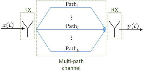
As shown in Fig. 1, we consider a point-to-point WPT system where an energy transmitter is intended to deliver energy wirelessly to an energy receiver, which is known as rectenna.
To reveal the most essential design insights, we assume that both the transmitter and receiver are equipped with a single antenna, while our design method can be similarly applied for the multi-antenna case. We assume that the available frequency band for WPT is continuous and given as , with and in Hz. Accordingly, we define and as the total bandwidth and the central frequency, respectively. Similar to the multisine waveform structure in [17], we assume that sinewaves are being used for WPT. We set their frequency tones as , , where and are designed such that is an integer and . In particular, we set and , with denoting the smallest integer greater than or equal to . Hence, the transmit signal over time is expressed as , with and , where and denote the amplitude and phase of the -th sinewave at frequency , respectively. In the rest of this paper, we treat ’s and ’s as design variables. It can be verified that is periodic, with the period . Moreover, the transmitter is subject to a maximum power constraint, denoted by , i.e.,
| (1) |
We consider that the transmitted signal propagates through a multipath channel, with paths, where the delay, amplitude, and phase for each path are denoted by , , , respectively. The signal received at the rectenna after multipath propagation is thus given by
| (2) |
where and are the amplitude and phase of the channel frequency response at , such that . In this paper, we assume the CSI, i.e., ’s and ’s, is known to the transmitter.
III Circuit Analysis of Rectenna
In this section, we present a simple and tractable nonlinear model of the rectenna circuit, and derive its output DC voltage as a function of the received signal by the rectenna.
III-A Rectenna Equivalent Circuit
As shown in Fig. 2, a typical rectenna consists of two main components, namely an antenna collecting EM waves (i.e., RF signals) from the air, and a single-diode rectifier converting the collected signal to DC for direct use or charging a battery. The antenna is commonly modelled as a voltage source in series with a resistance , where [17], with denoting the received signal as given in (2). On the other hand, the rectifier consists of a single diode, which is non-linear, followed by a LPF connected to an electric load, with the load resistance denoted by . As shown in Fig. 2, we denote as the equivalent input resistance of the rectifier. With the perfect impedance matching, i.e., , the input voltage of the rectenna, denoted by , is obtained as . Since is periodic, it follows that is also periodic with the same period .

Let and denote the current passing through the diode and the voltage drop across it, respectively. By assuming that the diode is ideal, we have
| (3) |
where is the reverse bias saturation current of the diode, is its thermal voltage, and is the ideality factor.
III-B Performance Analysis
By applying Kirchhoff’s circuit laws to the electric circuit of the rectifier shown in Fig. 2, we obtain
| (4) | ||||
| (5) | ||||
| (6) | ||||
| (7) |
where and are the output voltage and current of the rectifier, respectively, while and are the capacitance of the LPF and the current passing through it, respectively. After some manipulation based on (3)–(7), the relation between the input and output voltages of the rectifier is obtained as
| (8) |
Let , with and denoting the DC and AC (alternating current) components of the output voltage, respectively. Since the input voltage of the rectifier is periodic, it follows from (8) that is also periodic with the same period , i.e., for any integer . Moreover, the average value of is zero, i.e., . Next, by averaging both sides of (8) over the period , we obtain
| (9) |
By assuming that the capacitance of the LPF is sufficiently large, the output AC voltage of the rectifier is small, i.e., [17]. Hence, (9) can be simplified as
| (10) |
The DC power delivered to the load is thus given by
| (11) |
From (10), it is observed that its left hand side (LHS) is strictly increasing over . Thus, maximizing the output DC voltage/power is equivalent to maximizing the right hand side (RHS) of (10) by optimizing the received signal . Since is a function of the transmitted signal , we can alternatively design to achieve this goal. With the optimized and the resulted , we can evaluate the integration on the RHS of (10), and then use a bisection method to find satisfying (10). Such is unique, since the expression on the LHS of (10) is strictly increasing over .
It is worth noting that the existing approach to handle the integration on the RHS of (10) is to approximate the inner exponential function with its truncated Taylor series to the -th order as
| (12) |
where . The approximation in (12) is valid when is small. Specifically, , known as the linear model, is commonly adopted in the WPT and SWIPT/WPC literature (e.g., [6, 5]). The higher-order Taylor approximation model of the diode with has been recently considered in [17]. In contrast to the above studies, in this paper we avoid the Taylor approximation to ensure the best accuracy of the nonlinear EH model.
Last, note that to keep the output DC voltage constant over time, the capacitance of the LPF should be set such that , explained as follows. In the electric circuit of rectenna shown in Fig. 2, when the diode is reversely biased, the output voltage is governed by the discharging law of the capacitor of the LPF, and is proportional to . In this case, by setting e.g. , the normalized output voltage fluctuation (i.e., divided by the peak of the output voltage) is obtained as , which is reasonably small as practically required.
IV Problem Formulation and Proposed Solution
In this section, we formulate the waveform optimization problem. We then present two approximate solutions to it.
IV-A Problem Formulation
With the result in (10), we now proceed to optimize the sinewave amplitudes and phases, ’s and ’s, such that is maximized, under the maximum transmit sum-power constraint. The problem is formulated as
| (13) | ||||
| (14) |
with given in (2). To ensure that all terms in are being added constructively to each other, we need to set , . With this optimal phase design, in the rest of this paper, we focus on optimizing the sinewave amplitudes ’s by considering the following problem.
| (15) | ||||
| (16) |
The objective function and constraint in (15) and (16) are both convex over ’s. However, since maximizing a convex function over a convex set is non-convex in general, (P1) is a non-convex optimization problem. In the next subsections, we propose two approximate solutions to (P1).
Note that with the linear model of the diode or equivalently its second-order truncated Taylor approximation [1], the waveform optimization problem in (P1) can be simplified as a convex problem and then solved, where the obtained solution simply allocates all transmit power to the frequency tone with the largest channel magnitude, i.e., only , with , is being used for WPT. While with the higher-order truncated Taylor approximation model of the diode [17], (P1) can be simplified, but the resulted problem is still non-convex. In [17], the SCP technique is used to solve such non-convex problem approximately in an iterative manner, where a GP problem needs to be solved at each iteration.
IV-B Maximal Ratio Transmission (MRT) in Frequency Tones
Let . One approximate solution to (P1) is obtained by replacing the integral in (15) by the peak value of its integrand over one period , which is given by . To justify this approach, we present a numerical example as follows. We consider a SISO WPT with the center frequency kHz, the total bandwidth kHz, and the transmit power limit W. We set , kHz, and kHz. By considering a frequency-flat channel with , , we equally divide the transmit power over all frequency tones ’s, i.e., , . The details about rectenna circuit parameters are given later in Section V.

Accordingly, we plot in Fig. 3, from which it is observed that this signal has multiple large peaks in the vicinity of (and ms due to the periodicity), but has negligible amplitudes for rest of time . In this case, it seems reasonable to maximize the peak value of so as to approximately maximize its time average in (15). Thus, we reformulate (P1) as follows.
| (17) | ||||
| (18) |
(P2) is non-convex, but its optimal solution can be obtained by investigating its KKT conditions. We omit the details due to space limitation and present its optimal solution as follows.
Proposition IV.1
The optimal solution to (P2) is given by , .
The sinewave amplitudes ’s given in Proposition IV.1 can be considered as an approximate solution to the original problem (P1). Moreover, this solution is analogous to the MRT based beamforming in wireless communication, but applied in frequency domain instead of spatial domain.
IV-C Sequential Convex Programming (SCP) Based Solution
SCP is an iterative method to solve non-convex problems suboptimally, by leveraging convex optimization techniques. Specifically, at each iteration , , we approximate the objective function in (P1) by a linear function using its first-order Taylor series to form a convex approximate optimization problem. Next, we set the values of decision variables ’s for iteration as the optimal solution to the approximate problem at iteration . The algorithm continues until a given stopping criterion is satisfied. In the following, we provide details of our SCP based algorithm for (P1).
Let , , denote the values of decision variables at the beginning of iteration . We approximate the objective function in (15) via its first-order Taylor series as
| (19) |
with the coefficients given by
| (20) | ||||
| (21) |
where . Since the objective function in (15) is convex over ’s, the linear approximation given in (12) is its global under-estimator [18]. The integrals in (20) and (21) can be computed numerically as follows. Let be a large positive integer representing the number of sub-intervals of equal width used for signal sampling within the period , where denotes the duration of each sub-interval. By using the -point closed Newton-Cotes formula (also known as the trapezoidal rule) [19] to compute the integrals over each sub-interval , , and then adding up all the results, we can approximate (20) and (21) as
| (22) | ||||
| (23) |
for . Note that in the above, we have sampled each at equally spaced points. Let and , , denote the approximation errors. It can be shown that the error terms, and ’s, are all upper-bounded [19]. Specifically, we have and , , with and . It is observed that the errors are quadratically decreasing over . Hence, by setting sufficiently large, high-accuracy approximation can be achieved. In our algorithm, we set to obtain and ’s.11 1 To evaluate the actual value of the objective function of (P1) in (15) with our obtained solutions, we use the similar Newton-Cotes formula [19], but with a much larger number of samples per period to achieve the best accuracy.
Next, we present the approximate problem of (P1) for each iteration as follows.
| (24) | ||||
| (25) |
(P1) is a convex quadratically constrained linear programming (QCLP). The optimal solution to (P1) is given in the following proposition in closed-form.
Proposition IV.2
The optimal solution to (P1) is given by , .
We set ’s according to Proposition IV.2. We can then compute , and update . Let denote a presumed stopping threshold. If , then the algorithm terminates. Otherwise, if , then the algorithm will continue to the next iteration.
The above iterative algorithm is summarized in Table I, named SCP-QCLP algorithm. This algorithm cannot guarantee to converge to the optimal solution of the waveform optimization problem (P1), but can yield a point fulfilling the KKT conditions of (P1) [18]. Hence, SCP-QCLP algorithm returns (at least) a locally optimal solution to (P1).
SCP-QCLP Algorithm
- a)
Initialize , , , , and , , i.e., equal power allocation over all frequency tones.
- b)
- d)
Return ’s as the solution to (P1).
V Simulation Results
Consider a SISO WPT system, with central frequency MHz and total bandwidth MHz. For the channel from the energy transmitter to energy receiver, we assume dB path loss (i.e., they are separated by meters) in a large open space environment and a NLoS channel power delay profile with paths. For simplicity, we assume that the signal power is equally divided among all different paths. However, the delay of each path and its phase are assumed to be uniformly distributed over in s and , respectively. Fig. 4 shows one realization of the frequency response of the assumed channel, which will be used in the following simulations.


| Design approach | Convergence time (second) | ||
|---|---|---|---|
| SCP-QCLP | 0.014 | 0.033 | 0.425 |
| SCP-GP | 12.75 | 23.97 | 129.83 |
For the rectenna, the ohmic resistance of its antenna is set as , the parameters of its rectifier are given by A, mV, and , and its load resistance is set as k, same as in [17]. For SCP-QCLP algorithm in Table I, we set .
For comparison with our proposed frequency-MRT solution and SCP-QCLP algorithm, we consider two other benchmark designs: i) single-tone power allocation based on the linear model of the diode [1]; and ii) the SCP-GP algorithm [17] based on the higher-order truncated Taylor approximation model of the diode. To implement SCP-GP algorithm, we consider the -th order Taylor approximation model of the diode and set the relative error threshold as , the same as that considered for our SCP-QCLP algorithm. Moreover, we set the same initial point for both algorithms as , .
First, we fix . By varying the maximum transmit power limit , we plot the deliverable DC power in (11) under different waveform design schemes in Fig. 5. It is observed that SCP-QCLP achieves the best performance over all values of . It is also observed that the frequency-MRT solution considerably outperforms the conventional single-tone design for liner EH model. It is further observed that the gap between SCP-QCLP and SCP-GP increases with , explained as follows. In [17], SCP-GP is proposed based on the truncated Taylor approximation model of the diode, which is valid when the voltage drop across the diode, i.e., shown in Fig. 2, is small. However, by increasing the transmit power, the peak voltage collected by the rectenna increases, which causes the voltage drop across the diode to increase. As a result, the truncated Taylor approximation model of the diode becomes less accurate, and the performance of SCP-GP degrades. Furthermore, it is observed that the frequency-MRT solution achieves very close performance to both SCP-QCLP and SCP-GP, thus providing a practically appealing alternative design considering its low complexity.
Next, we fix W. By varying the number of utilized frequency tones for WPT, we plot the deliverable DC power under different waveform design schemes in Fig. 6. The convergence time of SCP-QCLP and SCP-GP is also compared in Table II.22 2 Simulations are implemented on MATLAB R2015b and tested on a PC with a Core i7-2600 CPU, 8-GB of RAM, and Windows 10. It is observed that SCP-QCLP achieves the best performance over all values of , and also converges remarkably faster than SCP-GP. This is due to the fact that SCP-QCLP requires only to solve a simple QCLP problem (with the optimal solution shown in closed-form in Proposition IV.2) at each iteration, while SCP-GP needs to solve a GP problem at each iteration, which requires more computational time. It is also observed that when increases, the frequency-MRT solution outperforms that by SCP-GP.
Last, with W and fixed, we plot the optimized sinewave amplitudes ’s for different designs as well as their corresponding signal waveform in Figs. 7(a)–(d), respectively.
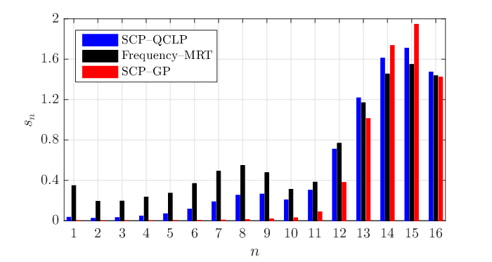


It is observed that under the frequency-MRT solution achieves the largest PAPR compared to the other two designs; however it has been shown in Figs. 5 and 6 that its deliverable DC power is less than those by SCP-QCLP and SCP-GP (when is not large). This is due to the fact that the deliverable DC voltage/power is proportional to the time average of the exponential function of the received RF signal (see (10)), but not depending on its peak value solely.
VI Conclusion
In this paper, we studied the waveform design problem for a SISO WPT system under frequency-selective channels assuming perfect CSI at energy transmitter. We developed a generic EH model based on circuit analysis that accurately captures the rectenna nonlinearity without relying on its Taylor approximation. Based on this model, we formulated a new multisine energy waveform optimization problem subject to a given transmit power constraint. Although the formulated problem is non-convex, we proposed two suboptimal solutions for it with low complexity. Simulation results showed the superiority of our proposed waveform solutions over the existing designs based on the truncated Taylor approximation in terms of both performance and computational time.
References
- [1] Y. Zeng, B. Clerckx, and R. Zhang, “Communications and signals design for wireless power transmission,” to appear in IEEE Trans. Commun., available online at arxiv/1611.06822.
- [2] G. A. Covic and J. T. Boys, “Inductive power transfer,” Proc. IEEE, vol. 101, no. 6, pp. 1276–1289, Jun. 2013.
- [3] A. Kurs, A. Karalis, R. Moffatt, J. D. Joannopoulos, P. Fisher, and M. Soljacic, “Wireless power transfer via strongly coupled magnetic resonances,” Science, vol. 317, no. 5834, pp. 83–86, Jul. 2007.
- [4] M. R. V. Moghadam and R. Zhang, “Multiuser wireless power transfer via magnetic resonant coupling: performance analysis, charging control, and power region characterization,” IEEE Trans. Sig. Inf. Process. Net., vol. 2, no. 1, pp. 72–83, Mar. 2016.
- [5] R. Zhang and C. K. Ho, “MIMO broadcasting for simultaneous wireless information and power transfer,” IEEE Trans. Wireless Commun., vol. 12, no. 5, pp. 1989–2001, May 2013.
- [6] H. Ju and R. Zhang, “Throughput maximization in wireless powered communication networks,” IEEE Trans. Wireless Commun., vol. 13, no. 1, pp. 418–428, Jan. 2014.
- [7] J. Xu and R. Zhang, “Energy beamforming with one-bit feedback,” IEEE Trans. Signal Process., vol. 62, no. 20, pp. 5370–5381, Oct. 2014.
- [8] Y. Zeng and R. Zhang, “Optimized training design for wireless energy transfer,” IEEE Trans. Commun., vol. 63, no. 2, pp. 536–550, Feb. 2015.
- [9] M. Xia and S. Aissa, “On the efficiency of far-field wireless power transfer,” IEEE Trans. Signal Procss., vol. 63, no. 11, pp. 2835–2847, Jun. 2015.
- [10] S. Bi and R. Zhang, “Distributed charging control in broadband wireless power transfer networks,” IEEE J. Sel. Areas Commun., vol. 34, no. 12, pp. 3380–3393, Dec. 2016.
- [11] G. Yang, C. K. Ho, R. Zhang, and Y. L. Guan, “Throughput optimization for massive MIMO systems powered by wireless energy transfer,” IEEE J. Sel. Areas Commun., vol. 33, no. 8, pp. 1640–1650, Aug. 2015.
- [12] S. Kashyap, E. Björnson, and E. G. Larsson, “On the feasibility of wireless energy transfer using massive antenna arrays,” IEEE Trans. Wireless Commun., vol. 15, no. 5, pp. 3466–3480, May 2016.
- [13] T. A. Khan, A. Alkhateeb, and R. W. Heath Jr, “Millimeter wave energy harvesting,” IEEE Trans. Wireless Commun., vol. 15, no. 9, pp. 6048–6062, Sep. 2016.
- [14] E. Boshkovska, D. W. K. Ng, N. Zlatanov, and R. Schober, “Practical non-linear energy harvesting model and resource allocation for SWIPT systems,” IEEE Commun. Letters, vol. 19, no. 12, pp. 2082–2085, Dec. 2015.
- [15] M. S. Trotter, J. D. Griffin, and G. D. Durgin, “Power-optimized waveforms for improving the range and reliability of RFID systems,” in Proc. IEEE Int. Conf. RFID, 2009.
- [16] A. Collado and A. Georgiadis, “Optimal waveforms for efficient wireless power transmission,” IEEE Microwave and Wireless Components Lett., vol. 24, no. 5, pp. 354–356, May 2014.
- [17] B. Clerckx and E. Bayguzina, “Waveform design for wireless power transfer,” IEEE Trans. Signal Process., vol. 64, no. 23, pp. 6313–6328, Dec. 2016.
- [18] S. Boyd and L. Vandenberghe, Convex Optimization. Cambridge, U.K.: Cambridge Univ. Press, 2004.
- [19] C. W. Ueberhuber, Numerical Computation 2: Methods, Software, and Analysis. Springer-Verlag, 1997.