Capacity Enhancement with Meta-Multiplexing

Multiplexing services as a key communication technique to effectively combine multiple signals into one signal and transmit over a shared medium. Multiplexing can increase the channel capacity by requiring more resources on the transmission medium. For instance, the space-division multiplexing accomplished through the multiple-input multiple-output (MIMO) scheme achieves significant capacity increase by the realized parallel channel, but it requires expensive hardware resources. Here, we present a novel multiplexing methodology, named meta-multiplexing, which allows ordinary modulated signals overlap together to form a set of “artificial” parallel channels; meanwhile, it only requires similar resources as ordinary modulation schemes. We prove the capacity law for the meta-multiplexing system and disclose that under broad conditions, the capacity of a single channel increases linearly with the signal to noise ratio (SNR), which breaks the conventional logarithmic growth of the capacity over SNR. Numerous simulation studies verify the capacity law and demonstrate the high efficiency of meta-multiplexing. Through proof-of-concept hardware experiments, we tested the proposed method in communication practices and achieved a spectral efficiency of 81.7 bits/s/Hz over a single channel, which is significantly higher than the efficiency of any existing communication system.

In the celebrated 1948 paper [1], Shannon derived the seminal formula for the capacity of the additive linear white Gaussian noise (AWGN) channel: $C=W\log_{2}(1+\mathrm{SNR})$, where the capacity $C$ is the tight upper bound of the rate at which information can be reliably transmitted over the channel, the capacity $C$ is determined by the bandwidth $W$ and the ratio of signal power to noise power SNR. People have made tremendous efforts to approach the ideal capacity limit [2]. The capacity of a single channel is hard to break, except for channels with nonlinearity [3, 4]. People also appeal to the multiplexing techniques [5, 6] to increase the capacity of a communication system by allocating more resources on the transmission medium: MIMO communication systems (see Fig. S1 in [7] ) establish a spatial parallel channel between the transmitter and receiver using multiple antenna pairs. The space-division multiplexing through the parallel channel significantly increases the capacity of MIMO systems. For instance, in an ideal situation, the capacity of a MIMO system is $N$ times larger than a single channel’s capacity, where $N$ is the smaller of the number of transmitter or receiver antennas. However, MIMO requires extra expensive radio frequency infrastructures and the availability of multiple independent channels, which may limit its applications. This paper introduces a novel multiplexing framework that incorporates ordinary modulated signals to construct an artificial parallel channel for a single physical channel without requiring much extra time or frequency resources. The proposed system requires more computation efforts but leads to a dramatic increase in the capacity. Under surprisingly broad conditions, such as various parameter setting for communication systems or even with interference from neighboring frequency bands, the system possesses a region in which the capacity increases linearly with the SNR. We named the system the meta-multiplexing, which is aligned to the “artificial” material “metamaterial” [8], as both utilize ordinary elements to form an “artificial” entirety and achieve extraordinary performance.

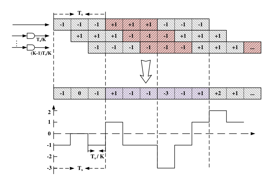
Recall that the enhanced capacity of the MIMO system is accomplished by the realized parallel channel derived from the channel matrix (see Fig. S1 in [7]). However, the channel matrix is leverage on the physical scattering propagation environment (independent uncorrelated spatial paths) and is difficult for humans to manipulate. In the meta-multiplexing, we construct the parallel channel artificially: assuming that the data is transmitted by symbols with symbol time $T$, Fig. 1A shows the naive idea of the meta-multiplexing scheme, in which we accelerate and parallel the transmission to $K$ streams and introduce a carefully designed time delay $T/K$ for each chain of the data stream. The multiple delays between different data streams are predefined; thus, the signals can be superposed together and propagate over a single physical channel, whereas at the receiver, unlike MIMO, we can decode them without requiring multiple antennas to capture different copies of the signal. We can further simplify the structure and process the multiplexing in the digital part as shown in Fig. 1B, which further reduces the cost of the implementation. We illustrate the meta-multiplexing process through a simple example shown in Fig. 2A. The binary phase-shift keying (BPSK) signal is paralleled and transmitted with a delay of $T/K$ for each stream. The summation of energy levels at each time slot $T/K$ produces the multiplexed signal, which is actually a waveform varying in one symbol time. Straightforwardly, the multiplexing process is equivalent to a convolution process in which the BPSK signal is convoluted with the rectangle waveform. Moreover, the pulse shaping filter $\textbf{h}(t)$ can be further extended to represent all of the impulse responses of the entire communication system, including the pulse shaping filter, the channel impulse response and the matched filter if available. Intuitively, the benefit of this scheme is that the data stream has been accelerated $K$ times and transmitted in $K$ parallel chains, and as a consequence, the information is carried by a novel format of waveform without requiring a great amount of extra transmission resources: no multiple antenna, no or limited extra bandwidth (discussed later) and only a negligible extra transmission time $(K-1)/K*T$.

To explore the capacity benefits of the meta-multiplexing precisely, we derive the capacity law for this communication scheme. As shown in Fig. 1C, the system can be represented by the matrix format $\mathbf{y}=\mathbf{H}\mathbf{x}+\mathbf{z}$, where vector $\mathbf{x}$ and $\mathbf{y}$ denotes the transmitted and received signal respectively, and $\mathbf{z}$ denotes the white Gaussian noise with variance $N$; $\mathbf{H}$ is a matrix in which each row is the impulse response coefficient $\mathbf{h}(t)$ shifted with a delay of $T/K$. By applying a singular value decomposition, $\mathbf{H}=\mathbf{U}\mathbf{\Lambda}\mathbf{V}$, with unitary matrix $\mathbf{U}$ and $\mathbf{V}$, and diagonal matrix $\mathbf{\Lambda}$, the matrix expression of the communication system is reformed as $\tilde{\mathbf{y}}=\mathbf{\Lambda}\tilde{\mathbf{x}}+\tilde{\mathbf{z}}$, where $\tilde{\mathbf{x}}$ , $\tilde{\mathbf{y}}$, and $\tilde{\mathbf{z}}$ are coordinate transformations of $\mathbf{x}$, $\mathbf{y}$, and $\mathbf{z}$ [6, 7]. The reformed expression clearly shows that the transmission system is equivalent to a parallel channel [6, 9]. Thus, by following the deduction of the capacity of the parallel channel [9], the capacity of the meta-multiplexing system can be obtained: $C=\frac{1}{2}\sum_{i=1}^{K}\log_{2}(1+\frac{P_{i}^{\ast}\lambda_{i}^{2}}{N})$ (bits/symbol), where $P_{i}^{\ast}$ are the waterfilling power allocations $P_{i}^{\ast}=\left(\mu-\frac{N}{\lambda_{i}^{2}}\right)^{+}$ in which $\mu$ is chosen to satisfy the power constraint $\sum_{i=1}^{K}P_{i}^{\ast}=P$ and $P$ is the total power allocated in one symbol time, and $\lambda_{1}$,…,$\lambda_{K}$, are the singular values of the matrix $\mathbf{H}$. A more detailed proof is presented in [7]. According to the formula of the capacity law, we obtain two important properties: 1) the capacity increases with the overlap factor $K$ because a number of $K$ non-zero $\lambda_{i}$ exists in the meta-multiplexing system [7], and each non-zero $\lambda_{i}$ corresponds to a sub-channel that can support the transmission of one data stream; 2) the capacity depends on the chosen waveform, because different waveforms generate significant different values for $\lambda_{i}$.

In communication practices, the energy per bit to noise power spectral density ratio $E_{b}/N_{0}$ (also known as the “SNR per bit”) is preferred to measure the condition of the communication without taking bandwidth into account. Denote the sampling period by $T_{s}$, and assume each data stream carries $\eta_{i}$ bits of information; then, the capacity over $E_{b}/N_{0}$ is $C=\frac{1}{2}\sum_{i=1}^{K}\log_{2}(1+\eta_{i}\frac{T_{s}}{T}\frac{E^{\ast}_{b,i}}{N_{0}}\lambda_{i}^{2})$, where $E^{\ast}_{b,i}=P_{i}^{\ast}T/\eta_{i}$ and $P_{i}^{\ast}$ is the waterfilling power allocation [7]. In practice, one simple but common setting is to divide the power evenly for each stream, $P_{i}=P/K$. In this case, the capacity becomes, $C_{I}=\frac{1}{2}\sum_{i=1}^{K}\log_{2}(1+\eta_{i}\frac{T_{s}}{T}\frac{E_{b}}{N_{0}}\lambda_{i}^{2})$. Regarding to the capacity law, we first investigate the capacity increasement with $K$. For simplicity, we choose a complex BPSK signal $(+1,-1,+j,-j)$ as the input for the meta-multiplexing system; thus, $\eta_{i}=2$. The capacity $C$ and $C_{I}$ are calculated and shown in Fig. 3A. The Shannon capacity curve is a special case of $C$ that $K=1$. To emphasize the linear relationship between capacity and $E_{b}/N_{0}$, the capacity is also displayed in a logarithmic scale. The numerical evaluation shows that $C_{I}$ is quite close to the ideal capacity $C$. Additionally, dividing the power evenly reduce the complexity and the cost of implementation of the meta-multiplexing scheme; thus, we use $C_{I}$ in the following discussion. To illustrate the capacity under different waveforms, two Taylor waveforms, a Gaussian waveform and a Hamming waveform, are evaluated and shown in Fig. S5 in [7]. It is obvious that the capacity of these waveforms is much smaller than that of the rectangle wave because (except for a few major ones) most of their singular values attenuate much faster than singular values of the rectangle wave. Therefore, the efficiency of the corresponding parallel channel is smaller than the rectangle wave. However, in any circumstance, when $K$ is sufficiently large, the capacity in a high SNR region can still increase linearly with the SNR.

The structure of this communication is not that complex, why does the community ignore it? One reason is that the meta-multiplexing scheme completely breaks the Nyquist intersymbol interference (ISI) criterion. The example depicted in Fig. 2A clearly shows the intersymbol interference. Generally, when ISI occurs due to various reasons such as the multipath propagation or bandlimit of a channel, people tend to mitigate the effects [6]. An alternative perspective is to utilize intersymbol interference to help the communication system, which dates back to the early 1970s [10]. However, few later works have had significant success. One noticeable work is the faster-than-Nyquist (FTN) signaling [11, 12], which intentionally builds a controlled amount of ISI into the communication system. A small amount of overlap on the symbols can carry more information with an increased sample rate. However, this strategy limits the overlap to less than half of a symbol duration. The overlapped multiplexing principle proposed in [13], further confirms that the overlapping between adjacent symbols can be a beneficial constraint with coding gain, but the overlap factor $K$ is limited to a small value. In this work, we push the limit of intersymbol “interference” so that we not only achieve impressive capacity when the overlap factor $K$ is sufficiently large but also disclose a capacity law that reveals the reason why the capacity increases with $K$.

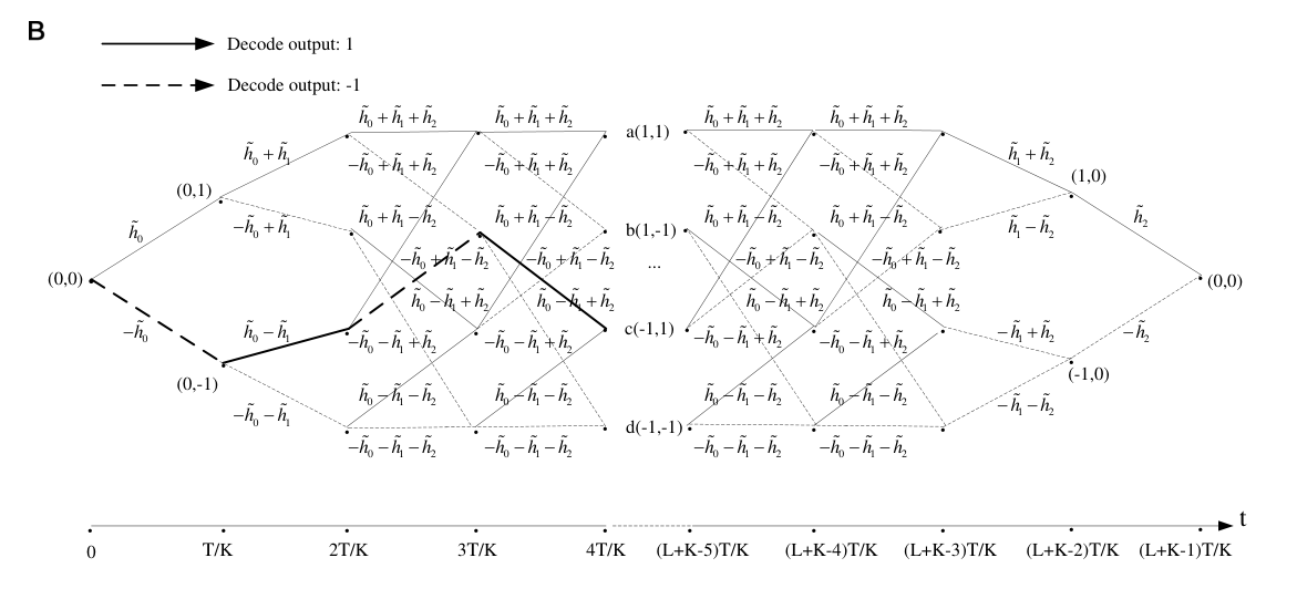
To design an entire communication system, conventional modules like synchronization and channel estimation are required; meanwhile, moderate modifications are needed to fit them into the meta-multiplexing system. The conventional FEC code scheme can be intergraded straightforwardly. One primary challenge lies in the decoding process of the multiplexed signal: how to decode the symbols, as they are heavily overlapped together. With regard to the convolution structure of the meta-multiplexing, a Viterbi-style algorithm is proposed. The trellis graph shows that the unknown information bits are one-to-one mappings of the trellis nodes, so decoding involves a dynamic search on the trellis graph (see Fig. 2B for a example of the decoded path on the trellis graph). However, the Viterbi-style algorithm can only deal with small $K$, as the decoding complexity increases exponentially with $K$. We further propose a Bayesian Monte Carlo [14, 15] based approximate decoding method. The proposed algorithm uses simulation-based techniques to simulate from a sequence of probability distributions for sequential inference of the posterior distribution of unknown information bits. The proposed algorithm provides a MAP decoding, whereas the complexity is independent of $K$ [7]. The algorithm has also been designed for parallel computing to support hardware implementation.

To simulate the transmission rate (bits per symbol) of the meta-multiplexing over different overlap factor $K$, we choose the complex BPSK signal as the input and the rectangle waveform as the pulse shaping filter. We set a series value for the overlap factor $K=[2,4,8,10,20,30,50,$ $60,100,200,300,450,600,900,1200,1800]$, and run the simulation study for $10^{6}$ bits. The Bayesian Monte Carlo decoding can support decoding even when $K$ is even larger than $1000$. For each $K$, we evaluate the level of $E_{b}/N_{0}$ that the system can gain the transmission rate of $2K$ bits/symbol with the bit error rate (BER) $\leq 10^{5}$. The simulated transmission rate in bits/symbol over $E_{b}/N_{0}$ is shown in Fig. 3A. Obviously, the simulation results support that the realized transmission rate is linearly proportional to the $E_{b}/N_{0}$. The discrepancy between the realized transmission rate and the theoretical capacity can be further reduced with the help of a near-capacity forward error correcting (FEC) coding scheme, such as turbo code [16] and LDPC [17, 18]. A twofold FEC coding mechanism is applied in our meta-multiplexing system (see Fig. S1 in [7]): the convolution structure of the meta-multiplexing serves as the inner “convolutional” coding, which is a noticeable advantage of our system. For outer FEC coding, we choose a $3/5$ code rate LDPC from the DVB-S.2 standard. An interleaving algorithm is inserted between the inner and outer coding. Simulation studies in Fig. 3A illustrate that with the help of LDPC coding, the realized transmission rate moves approximately 4dB closer to the theoretical capacity curve.

The symbol, mentioned in previous discussion, actually represents a two-dimensional resource containing both the time duration and the frequency bandwidth. However, the dilemma is that for any spectrum bandlimited signal, its waveform is not realizable, and for any realizable waveform, its absolute bandwidth is infinite. In engineering practices, various definitions of the bandwidth for the realizable waveform have been proposed to describe the power distribution of the signal [7]. In the meta-multiplexing system, one important property is that the multiplexed signal follows the occupied bandwidth of the pulse shaping filter: the convolution structure of the meta-multiplexing decides that the bandwidth of the multiplexed signal is concentrated and generally less than the bandwidth of the pulse shaping filter. Fig. S4 verifies the spectrum property of the meta-multiplexing signal [7]. Given the symbol’s occupied bandwidth $B$, the capacity of the meta-multiplexing can be expressed as $\eta=\frac{1}{2BT}\sum_{i=1}^{K}\log_{2}(1+\frac{P_{i}\lambda_{i}^{2}}{N})$ ( or $\frac{1}{2BT}\sum_{i=1}^{K}\log_{2}(1+\eta_{i}\frac{T_{s}}{T}\frac{E_{b}}{N_{0}}\lambda_{i}^{2})$ for the measurement by $E_{b}/N_{0}$) (bits/s/Hz) [7]. The normalized capacity (or spectral efficiency) is proportional to the capacity with a coefficient $1/BT$. In a similar setting as discussed before, we simulated the spectral efficiency $E_{b}/N_{0}$. The resulting spectral efficiency (in Fig. 4A) shows that the curve moves to the right compared with the capacity curve because that the occupied bandwidth is always larger than $1/T$, and thus, the coefficient $1/BT<1$.

According to the Nyquist-Shannon sampling theorem [1], the processing bandwidth (the reciprocal of the sampling rate) of a communication signal is at least two times larger than the occupied bandwidth. In the meta-multiplexing, the processing bandwidth becomes much larger than the occupied bandwidth, particularly when $K$ is large (shown in Fig. S5 in [7]). A concern of this multiplexing scheme is how to understand the “problematic” spectrum region that is outside of the occupied bandwidth but inside of the processing bandwidth. Here, we provide a convincing way to eliminate this concern: when the “problematic” spectrum region is occupied by other communication signals, either meta-multiplexing signals or ordinary ones, the meta-multiplexing system can still work properly. Fig. S6 in [7] shows an example in which one 256-QAM signal exits in the processing bandwidth of a meta-multiplexing signal. We define the bounded PSD at 35 dB as the occupied bandwidth; then, the meta-multiplexing signal occupies a bandwidth of 31.6 KHz, while the QAM occupies 750 KHz approximately $75\%$ of the entire processing bandwidth of 1 MHz. A joint decoding strategy is proposed to decode the signal (see [7] for details). The simulated spectral efficiency requires approximately 2 dB higher $E_{b}/N_{0}$ than the one without any neighboring signal in the processing bandwidth, but the linear relation with the $E_{b}/N_{0}$ still holds (see the spectral efficiency with spectrum sharing for different $K$ in Fig. 4A). Consequently, we can measure the spectral efficiency of the meta-multiplexing only on its occupied bandwidth, and then, the resulting spectral efficiency is consistent linear increase with the SNR, as we discussed previously. Moreover, the proposed scenario bring a smart strategy for the cognitive radio community[19, 20], in which the licensed primary users of the spectrum use the QAM, while the secondary users use the spectrum without interrupt and interaction with primary users.

Moreover, to verify that the meta-multiplexing works in real-world physical channels, we implemented the entire communication system on a standard verification system, the universal software radio peripheral (USRP). The placement of the connection of the USRP devices is shown in Fig. S7 in [7]. All of the algorithms were implemented on the onboard high-performance field-programmable gate array (FPGA). We set $K=128$ and choose the Taylor waveform with an attenuation level of -35dB for the pulse shaping filter [7]. The artificial delay $T/K$ is 1 millisecond. The meta-multiplexing signal is up-converted to radio frequency at 2.4 Ghz. The spectrum of the channel signal is measured by the spectrum analyzer and displayed in Fig. S8: the measured occupied bandwidth of the channel signal is 24.48 KHz. The noise generator add the Gaussian noise to the channel to evaluate the BER performance. A pilot signal is utilized to estimated the channel conditions for equalization before decoding. We engineer the Bayesian Monte Carlo based approximate decoding algorithm in a parallel style, which can fit the FPGA implementation. Accordingly, all of the defects of a real physical communication system, like analog-to-digital converter (ADC)/digital-to-analog converter (DAC) quantization errors and nonlinearity of the power amplifier, exist in this verification. As shown in Fig. 4B, the dispersion between the simulation and hardware implementation is caused by the effective number of bits (ENOB) of ADC and DAC in the system. The BER of this hardware implementation, which is highly consistent with the simulation with ENOB=12, confirms that the proposed meta-multiplexing works in practical communication systems. We utilized a 24.48 KHz bandwidth but realized a reliable transmission ($\verb"BER"<10^{-5}$) of 2M bits/sec in the $E_{b}/N_{0}$ region of 45 dB, so the spectral efficiency is up to 81.7 bits/s/Hz, which is significantly higher than the efficiency of any existing communication system. Actually, such a high spectral efficiency is generally infeasible for conventional communication methods like high-order QAM modulations: the required ADC and DAC ENOB should be larger than 40, and the required $E_{b}/N_{0}$ should be more than 230 dB, all of which are beyond the physical ability of conventional communication systems.

The meta-multiplexing strategy can also be applied in other domains, such as the frequency domain and joint time-frequency domain, to create other novel multiplexing methods. Take meta-multiplexing in frequency as an example: the superposition in frequency would save bandwidth and benefit broadband communication applications. The proposed communication framework is suitable for different channel conditions. For example, in the multipath Rayleigh fading channel, the random time dispersion of the channel can be treated as part of the entire pulse response $\textbf{h}(t)$, and blind deconvolution techniques can be employed for the decoding when part of $\textbf{h}(t)$ is unknown. As a general multiplexing technique offering significant capacity enhancement, meta-multiplexing will bring new possibilities for modern communications jointly with current communication technologies.

• 1.

  We thank Prof. Daoben Li, Junbi Chen for their helpful discussions and kind suggestions, Dr. Changwei Lv, Chao Fang for their assistance for the experimental apparatus.

References and Notes

- [1] C. E. Shannon, Bell Syst. Tech. J. 27, 379 (1948).
- [2] D. J. Costello, G. D. Forney, Proceedings of the IEEE 95, 1150 (2006).
- [3] P. P. Mitra, J. B. Stark, Nature 411, 1027 (2001).
- [4] M. Sorokina, S. Turitsyn, Nature Communications (2014).
- [5] J. G. Proakis, Digital Communications 4th edition (New York: McGraw Hill, 2001).
- [6] D. Tse, P. Viswanath, Fundamentals of Wireless Communication (Cambridge University Press, 2005).
- [7] Materials and methods are available as supporting material.
- [8] R. Liu, et al., Science 323, 366 (2009).
- [9] T. M. Cover, J. A. Thomas, Elements of Information Theory (John Wiley & Sons, Inc., 2006).
- [10] G. Forney, IEEE Trans. Inf. Theory 18(3), 363 (1972).
- [11] J. E. Mazo, Bell Syst. Tech. 54, 1451 (1975).
- [12] D. Dasalukunte, V. Owall, F. Rusek, J. Anderson, Faster than Nyquist Signaling (Springer-Verlag, 2014).
- [13] D. Li, A High Spectral Efficient Waveform Encoding OVTDM Theory and Applications (China Academic Press, 2013).
- [14] A. Doucet, J. F. G. De Freitas, N. J. Gordon, eds., Sequential Monte Carlo in Practice (Springer Verlag, New York, 2001).
- [15] J. Liu, Monte Carlo Strategies in Scientific Computing (Springer-Verlag, New York, 2001).
- [16] C. Berrou, A. Glavieux, P. Thitimajshima, Proc. 1993 Int. Conf. Commun. (Geneva) pp. 1064–1070 (1993).
- [17] D. J. C. MacKay, R. M. Neal, Elect. Lett. 32, 1645 (1996).
- [18] R. G. Gallager, Low-Density Parity-Check Codes (MA: MIT Press, 1963).
- [19] J. Mitola, G. Maguire, IEEE Personal Communications 6, 13 (1999).
- [20] B. Wang, K. Liu, IEEE J. Sel. Topics Signal Process. 5, 5 (2011).
- [1] D. Tse and P. Viswanath, Fundamentals of Wireless Communication (Cambridge University Press, 2005).
- [2] T. Cover and J. Thomas, Elements of Information Theory(John Wiley & Sons, Inc., 2006).
- [3] M. Loeve, Probability Theory (Springer, 1977).
- [4] B. Sklar, Digital Communications: Fundamentals and Applications (Prentice Hall, 2001).
- [5] N. J. Gordon, D. J. Salmond and A. F. M. Smith, IEE Proceedings F, Radar and Signal Processing, 140, 107(1993).
- [6] J. S. Liu, Monte Carlo Strategies in Scientific Computing (Springer, New York, 2001).
- [7] A. Doucet, J. F. G. De Freitas and N. J. Gordon, Sequential Monte Carlo Methods in Practice(Springer, New York, 2001).
- [8] A. Athalye, M. Bolic, S. Hong and P. M. Djuric, EURASIP Journal on Advances in Signal Processing, 2005(17), 2888(2005).
- [9] N. Kantas, A. Doucet, S. S. Singh, J. Maciejowski and N. Chopin, Statistical Science, 30, 328(2015).
Fig. S1. Schematic of a MIMO system: the information bits are formatted into multiple streams, transmitted through transmission antennas and a multipath channel, and received by receiver antenna. The MIMO system can be expressed as , where the matrix represents the physical paths between the transmitter and the receiver [1].
![[Uncaptioned image]](1703.03989v2/ovt_channel.png)
Fig. S2. The framework of a meta-multiplexing communication system. Conventional communication modules like FEC coding, synchronization and channel estimation requires only moderate modification to fit into the meta-multiplexing system.
Fig. S3. The meta-multiplexing system can be converted into a parallel channel through singular value decomposition [1].
(A)
(B)
(C)
Fig. S4. (A) Basic waveforms in time domain. (B) Spectrum of the basic waveforms; dotted lines show the bound PSD bandwidth of Taylor waveforms. (C) Spectrum of the meta-multiplexing signal with and data length; dotted lines show the bound PSD bandwidth, while dash lines the processing bandwidth.
![[Uncaptioned image]](1703.03989v2/wave_comp.png)
![[Uncaptioned image]](1703.03989v2/taylor50_symbol.png)
Fig. S5. (A) The capacity of meta-multiplexing systems with different waveforms. (B) The capacity and the realized transmission rate of the meta-multiplexing system, which uses the Taylor waveform with an attenuation level of -50 dB as the pulse shaping filter.
![[Uncaptioned image]](1703.03989v2/spectrum_share.png)
Fig. S6. Plot of the spectrum sharing scheme. The meta-multiplexing use an overlap factor K=100 and a Taylor waveform with an attenuation level of -35 dB. One 256-QAM signal occupies approximately 75% of the processing bandwidth of the meta-multiplexing signal.
Fig. S7. The connectivity of the USRP devices for hardware verification.
![[Uncaptioned image]](1703.03989v2/measure.png)
Fig. S8. Measure the frequency response of the meta-multiplexing signal in the real physical channel by a spectrum analyzer. The signal is rolled off to -35dB in a bandwidth of 24.48 KHz.