Level crossings and excess times due to a super-position of uncorrelated exponential pulses

The FPP can be described as a super-position of uncorrelated pulses, [2, 8, 30, 40, 26, 19, 25, 27, 28, 29, 1, 41, 32, 33]

$$\Phi_{K}(t)=\sum_{k=1}^{K(T)}A_{k}\varphi\left(\frac{t-t_{k}}{\tau_{\text{d}}}\right),$$

(7)

where for event $k$, $t_{k}$ is the pulse arrival time and $A_{k}$ is the pulse amplitude. The pulse duration time $\tau_{\text{d}}$ and the pulse shape $\varphi(x)$ are assumed to be the same for all events. We will assume the waiting time between pulses to be uncorrelated and exponentially distributed with mean waiting time $\tau_{\text{w}}$. From this it follows that $K(T)$ is Poisson distributed with constant rate $1/\tau_{\text{w}}$,

$$P_{K}(K)=\frac{1}{K!}\left(\frac{T}{\tau_{\text{w}}}\right)^{K}\exp\left(-\frac{T}{\tau_{\text{w}}}\right),$$

(8)

and therefore that the pulse arrival times $t_{k}$ are uniformly distributed on $[0,T]$.

In the following, the pulse shape is described by a two-sided exponential function

$$\varphi(x)=\begin{cases}\exp{\left(x/\lambda\right)},&\quad x<0,\\ \exp{\left(-x/(1-\lambda)\right)},&\quad x\geq 0,\end{cases}$$

(9)

where $\lambda$ is a pulse asymmetry parameter restricted to the range $0<\lambda<1$. The ratio between the pulse duration and average waiting time,

$$\gamma=\frac{\tau_{\text{d}}}{\tau_{\text{w}}},$$

(10)

is called the intermittency parameter, and determines the degree of pulse overlap. It is the most fundamental parameter of the stochastic model. Realizations of this process for various values of $\gamma$ are shown in Fig. 1, using the normalization given in Eq. (3). For small $\gamma$, the pulses are well separated and the process is strongly intermittent. For large $\gamma$, there is significant pulse overlap and realizations of the process resembles random noise, with relatively small and symmetric fluctuations around the mean value. For intermediate $\gamma$, large-amplitude bursts can be constructed from one separate large-amplitude pulse, or several smaller amplitude pulses. Because of this, the parameter $\gamma$ can be interpreted as an intermittency parameter for the process, with low values of $\gamma$ giving a highly intermittent process and high values of $\gamma$ giving a weakly intermittent process.

Assuming the PDF of the pulse amplitudes $A$ is an exponential distribution,

$$P_{A}(A)=\frac{1}{\left<A\right>}\exp\left(-\frac{A}{\left<A\right>}\right),\,A>0,$$

(11)

the stationary distribution of the random variable $\Phi(t)$ can be shown to be a Gamma distribution with shape parameter $\gamma$ and scale parameter $\left<A\right>$;[42, 16, 8, 30, 35]

$$P_{\Phi}(\Phi)=\frac{1}{\left<A\right>\Gamma(\gamma)}\left(\frac{\Phi}{\left<A\right>}\right)^{\gamma-1}\exp\left(-\frac{\Phi}{\left<A\right>}\right),\,\Phi>0,$$

(12)

where $\Gamma(x)$ is the gamma function.[39] The complementary CDF of $\Phi$ is then given by

$$1-C_{\Phi}(\Phi)=Q\left(\gamma,\gamma\Phi/\left<\Phi\right>\right),$$

(13)

where $Q(a,x)$ is the regularized upper incomplete gamma function with parameter $a$.[39] In this contribution, we will also use the upper incomplete gamma function $\Gamma(a,x)$.[39] $Q(a,x)$ is defined as $Q(a,x)=\Gamma(a,x)/\Gamma(a)$.

The complementary CDF of $\Phi$ as a function of $\widetilde{\Phi}$ for various values of $\gamma$ is presented in Fig. 2. This function can be interpreted as the fraction of time a signal spends above the threshold $\widetilde{\Phi}$. As $\gamma$ increases, the PDF approaches a normal distribution. In the normal regime $\gamma\gg 1$, the fraction of time above threshold falls rapidly with increasing threshold level since the fluctuations in the signal are concentrated around the mean value. In the strong intermittency regime, $\gamma\ll 1$, the signal spends long periods of time close to zero value as few pulses overlap significantly. Thus, the total time above threshold increases rapidly as the threshold approaches zero. Also note that for large values of $\Phi$, the total time above threshold is orders of magnitude higher for a process with high intermittency than for a process with low intermittency. For $\gamma=1$, the PDF of $\Phi$ is an exponential distribution.

Correspondingly, the characteristic function of $\Phi$ is

$$\left<{\exp(i\Phi u)}\right>=(1-i\left<A\right>u)^{-\gamma}.$$

(14)

It can likewise be shown that the cumulants of the process for arbitrary pulse shape and amplitude distribution are given by[8, 30]

$$\kappa_{n}=\gamma\left<{A}^{n}\right>I_{n},$$

(15)

where

$$I_{n}=\int\limits_{-\infty}^{\infty}\text{d}x\,\left[\varphi(x)\right]^{n}.$$

(16)

For the pulse shape given in Eq. (9), $I_{n}=1/n$ and using that $\langle{A^{n}}\rangle=n!\,\left<A\right>^{n}$ for exponentially distributed amplitudes, the cumulants for $\Phi$ are[8, 30]

$$\kappa_{n}=(n-1)!\,\gamma\left<A\right>^{n}.$$

(17)

Note that the cumulants, and therefore also the PDF, are independent of the pulse asymmetry parameter $\lambda$. Given the cumulants, we can find the lowest order moments of the process:[2, 42, 8, 30]

	$\displaystyle\left<\Phi\right>$	$\displaystyle=\gamma\left<A\right>,$		(18a)
	$\displaystyle\Phi_{\text{rms}}^{2}$	$\displaystyle=\gamma\left<A\right>^{2},$		(18b)
	$\displaystyle S_{\Phi}$	$\displaystyle=\frac{2}{\gamma^{1/2}},$		(18c)
	$\displaystyle F_{\Phi}$	$\displaystyle=3+\frac{6}{\gamma}.$		(18d)

Here, $S_{\Phi}$ is the skewness of the random variable $\Phi$, and $F_{\Phi}$ is its flatness. The relative fluctuation level is $\Phi_{\text{rms}}/\left<\Phi\right>=1/\gamma^{1/2}$. There is a parabolic relation between skewness and flatness: $F_{\Phi}\left(S_{\Phi}\right)=3+3S_{\Phi}^{2}/2$. It can be shown that the distribution of the normalized process $\widetilde{\Phi}=(\Phi-\left<\Phi\right>)/\Phi_{\text{rms}}$ resembles a standard normal distribution (that is, a normal distribution with zero mean and unit standard deviation) in the limit $\gamma\to\infty$, independent of pulse shape and amplitude distribution.[2] In this case, both the skewness $S_{\Phi}$ and the excess kurtosis $F_{\Phi}-3$ vanish.[2, 8] Conversely, for $\gamma\to 0$, the skewness and kurtosis moments both tend to infinity. Note that from the definition of skewness and flatness, it follows that $S_{\Phi}=S_{\widetilde{\Phi}}$ and $F_{\Phi}=F_{\widetilde{\Phi}}$.

Note that $\Phi$ is non-negative, giving $\widetilde{\Phi}\geq-\gamma^{1/2}$. By contrast, a normally distributed random variable has infinite support. The difference between the PDF of $\widetilde{\Phi}$ and a standard normal distribution due to this discrepancy is negligible in practice, since values of $-\gamma^{1/2}$ or less are highly unlikely for a standard normal distribution in the case of $\gamma\gg 1$.

In order to calculate the joint distribution of the process and its derivative, the normalized time derivative is defined by

$$\Theta_{K}(t)=\frac{\tau_{\text{d}}}{2}\frac{\text{d}\Phi_{K}}{\text{d}t}=\sum_{k=1}^{K(T)}A_{k}\vartheta{\left(\frac{t-t_{k}}{\tau_{\text{d}}}\right)},$$

(19)

where the pulse shape is given by

$$\vartheta(s)=\frac{1}{2}\frac{\text{d}\varphi}{\text{d}s}=\frac{1}{2}\begin{cases}(\lambda)^{-1}\exp{\left(s/\lambda\right)},&\quad s<0,\\ -(1-\lambda)^{-1}\exp{\left(-s/(1-\lambda)\right)},&\quad s\geq 0.\\ \end{cases}$$

(20)

Here, we have divided by a factor 2 in order for the pulse shape to fulfill $\int_{-\infty}^{\infty}\text{d}s\,{\left|\vartheta(s)\right|}=1$.¹¹ 1 This is a correction to $\vartheta$ given in . This leads to corrections in the rms-value of $\Theta$ and the joint PDF between $\Phi$ and $\Theta$, but not the excess statistics. This is another stochastic process of the same type as that given in Eq. (7), but with a different pulse shape. Since the process $\Phi(t)$ is stationary, it follows that $\left<{\Theta}\right>=0$, which is easily verified from Eq. (17). The processes $\Phi(t)$ and $\Theta(t)$ are evidently dependent yet also uncorrelated,

$$\left<{\Phi\Theta}\right>=\frac{\tau_{\text{d}}}{4}\frac{\text{d}}{\text{d}t}\left<{\Phi^{2}}\right>=0.$$

(21)

In Appendix A, the joint PDF between $\Phi$ and $\Theta$ is used to demonstrate that $\Phi$ and $\Theta$ become independent in the limit $\gamma\to\infty$.

The lowest order moments of $\Theta$ are readily calculated as

	$\displaystyle\left<\Theta\right>$	$\displaystyle=0,$		(22a)
	$\displaystyle\Theta_{\text{rms}}^{2}$	$\displaystyle=\gamma\left<A\right>^{2}/\left[4\lambda(1-\lambda)\right],$		(22b)
	$\displaystyle S_{\Theta}$	$\displaystyle=2(1-2\lambda)/[\gamma\lambda(1-\lambda)]^{1/2},$		(22c)
	$\displaystyle F_{\Theta}$	$\displaystyle=3+6[1+(1-2\lambda)^{2}/\lambda(1-\lambda)]/\gamma.$		(22d)

In the limit of $\lambda\to 0$ or $\lambda\to 1$, the moments $\Theta_{\text{rms}}$, $S_{\Theta}$ and $F_{\Theta}$ diverge, meaning the PDF of $\Theta$ does not exist in this case. In these limits, the pulse shape in $\Phi$ is discontinuous and the derivative of the pulse shape contains delta functions. Thus we require the two-sided exponential pulse shape to calculate the rate of level crossings. It will later be shown that these limits exist for the rate of level crossings and are consistent with other methods starting from the one-sided exponential pulse shape. Thus, while this method cannot be used to calculate the rate of level crossings for a discontinuous signal, the rate still exists.[12, 16, 18]

Using the same approach as in Refs. 8 and 30, the characteristic function of $\Theta$ is given by

$$\left<{\exp(i\Theta v)}\right>=\left(1-i\left<A\right>\frac{v}{2\lambda}\right)^{-\lambda\gamma}\left(1+i\left<A\right>\frac{v}{2(1-\lambda)}\right)^{-(1-\lambda)\gamma}.$$

(23)

This characteristic function can be interpreted as originating from the sum of two independent gamma distributed variables, one over positive values with shape parameter $\gamma\lambda$ and scale parameter $\left<A\right>/(2\lambda)$, and the other over negative values with shape parameter $\gamma(1-\lambda)$ and scale parameter $\left<A\right>/[2(1-\lambda)]$. The PDF of this compound process is a convolution of the two gamma distributions, which to the best of the authors knowledge does not have a closed form. Still, the argument in Refs. 2, 8, 30 applies here as well, and the PDF of $\Theta$ resembles a normal distribution in the limit $\gamma\to\infty$. In Fig. 3, realizations for $\widetilde{\Theta}$ are presented for $\lambda=1/4$ and various values of $\gamma$. Arrival times and pulse amplitudes are the same as in Fig. 1. Again, the process is strongly intermittent for low values of $\gamma$, and resembles random noise for high values of $\gamma$.

By choosing $\lambda=1/2$, the pulse shape $\varphi(x)$ is symmetric. In this case, the characteristic function in Eq. (23) has an inverse transformation in closed form, and the corresponding PDF is given by

$$P_{\widetilde{\Theta}}(\widetilde{\Theta})=\sqrt{\frac{2\gamma}{\pi}}\frac{2^{-\gamma/2}}{\Gamma(\gamma/2)}{\left|\sqrt{\gamma}\widetilde{\Theta}\right|}^{(\gamma-1)/2}\mathcal{K}_{(\gamma-1)/2}\left({\left|\sqrt{\gamma}\widetilde{\Theta}\right|}\right),$$

(24)

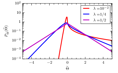
where $\mathcal{K}_{a}(x)$ is the modified Bessel function of the second kind.[39] This PDF is presented in Fig. 4 for various values of $\gamma$. For small values of $\gamma$, this PDF has exponential tails and is sharply peaked at the mean value, while it resembles a normal distribution for large values of $\gamma$. The same PDF for $\gamma=2$ and various values of $\lambda$ is presented in Fig. 5. As the asymmetry parameter approaches $0$, the skewness and flatness of $\Theta$ increases. It can be seen from Eq. (23) that in the case $\lambda=1/2$ and $\gamma=2$, $\Theta$ is symmetrically Laplace distributed with zero mean and standard deviation $\Theta_{\text{rms}}=2\left<A\right>^{2}$.[44]

The joint PDF of $\Phi$ and $\Theta$ is generally given by

$$P_{\Phi\Theta}\left(\Phi,\Theta\right)=\frac{1}{\left(2\pi\right)^{2}}\int\limits_{-\infty}^{\infty}\text{d}u\,\int\limits_{-\infty}^{\infty}\text{d}v\,\exp\left(-i\Phi u-i\Theta v\right)\left<{\exp\left(iu\Phi+iv\Theta\right)}\right>.$$

(25)

Using that individual events are uncorrelated and that the number of pulses is Poisson distributed, the characteristic function of $\Phi$ and $\Theta$ can be calculated as

$$\left<{\exp\left(iu\Phi+iv\Theta\right)}\right>=\exp\left(\gamma\int\limits_{-\infty}^{\infty}\text{d}AP_{A}(A)\,\int\limits_{-\infty}^{\infty}\text{d}s\,\left[\exp\left(iuA\varphi(s)+ivA\vartheta(s)\right)-1\right]\right).$$

(26)

This expression is given in Refs. 33, 37 for the case of fixed (degenerately distributed) pulse amplitudes, although the generalization is straightforward. Exchanging the order of integration, we find that

$$\left<{\exp(iu\Phi+iv\Theta)}\right>=\left[1-i\left<A\right>\left(u+\frac{v}{2\lambda}\right)\right]^{-\gamma\lambda}\left[1-i\left<A\right>\left(u-\frac{v}{2(1-\lambda)}\right)\right]^{-\gamma\left(1-\lambda\right)}.$$

(27)

We note that we recover the expression for the characteristic function of $\Phi$ in Eq. (14) by setting $v=0$ in this equation, and we recover the characteristic function of $\Theta$ in Eq. (23) by setting $u=0$. Substituted into Eq. (25), the stationary joint PDF can be obtained in closed form. We change variables to $x=\left<A\right>[u+v/(2\lambda)]$ and $y=\left<A\right>\{u-v/[2(1-\lambda)]\}$, and use the notation

	$\displaystyle\alpha$	$\displaystyle=\frac{\lambda}{\left<A\right>}\left[\Phi+2(1-\lambda)\Theta\right],$
	$\displaystyle\beta$	$\displaystyle=\frac{1-\lambda}{\left<A\right>}\left(\Phi-2\lambda\Theta\right).$

The joint PDF can now be written as

$$P_{\Phi\Theta}\left(\Phi,\Theta\right)=\frac{2\lambda(1-\lambda)}{\left(2\pi\left<A\right>\right)^{2}}\int\limits_{-\infty}^{\infty}\text{d}x\,\left[1-ix\right]^{-\gamma\lambda}\exp\left(-i\alpha x\right)\int\limits_{-\infty}^{\infty}\text{d}y\,\left[1-iy\right]^{-\gamma(1-\lambda)}\exp\left(-i\beta y\right).$$

(28)

The integrals can be performed separately, and we get the closed form expression

$$P_{\Phi\Theta}{\left(\Phi,\Theta\right)}=\frac{2\gamma^{\gamma}\lambda^{\gamma\lambda}(1-\lambda)^{\gamma(1-\lambda)}}{\left<\Phi\right>^{\gamma}\Gamma(\gamma\lambda)\Gamma{\left(\gamma(1-\lambda)\right)}}\exp\left(-\frac{\gamma\Phi}{\left<\Phi\right>}\right)\left[\Phi+2(1-\lambda)\Theta\right]^{\gamma\lambda-1}\left(\Phi-2\lambda\Theta\right)^{\gamma(1-\lambda)-1}.$$

(29)

This is non-zero only for the limited range $-\Phi/[2(1-\lambda)]<\Theta<\Phi/(2\lambda)$, which follows from the fact that the signal $\Phi(t)$ cannot decrease faster than the rate of decay of individual pulse structures, nor increase slower than the rate of growth of individual pulses, since the pulse amplitudes are positive definite. The dependence between $\Phi$ and $\Theta$ is evident from Eq. (29), since the joint PDF is not separable into a product of the marginal PDFs. As expected, $P_{\Phi}(\Phi)$ can be recovered by integrating over $\Theta$. Also note that the expression for the joint PDF diverges in the limits $\lambda\to 0$ and $\lambda\to 1$, as was the case for the moments and PDF of $\Theta$. As the PDFs of both $\Phi$ and $\Theta$ resemble normal distributions in the limit $\gamma\to\infty$ and they are uncorrelated, the joint PDF for $\Phi$ and $\Theta$ resembles the product of two normal distributions, that is, a joint normal distribution with vanishing correlation coefficient. This is demonstrated explicitly in Appendix A. Thus, in the normal limit $\gamma\to\infty$, the classical Rice formula given by Eq. (2) is recovered. As in the case of $P_{\Phi}$, there is a discrepancy between $P_{\Phi\Theta}$ and a joint normal distribution due to the limited region of non-zero values of $P_{\Phi\Theta}$. The domain of non-zero values can be written as $-(\widetilde{\Phi}+\gamma^{1/2})/(1-\lambda)<\widetilde{\Theta}/\sqrt{\lambda(1-\lambda)}<(\widetilde{\Phi}+\gamma^{1/2})/\lambda$, where $\widetilde{\Theta}=\Theta/\Theta_{\text{rms}}$. For standard normally distributed variables, values outside of this domain are highly unlikely in the case of $\gamma\gg 1$, and this discrepancy is in practice negligible.

The joint distribution $P_{\Phi\Theta}(\Phi,\Theta)$ is presented in Fig. 6 for $\gamma\in\{10^{-1},1,10\}$ and $\lambda\in\{1/4,1/2\}$. It should be noted that logarithmic scaling is used for $\gamma=10^{-1}$ and $1$, while linear scaling is used for $\gamma=10$. The white area in all figures are the regions where $P_{\Phi\Theta}$ vanishes, as given by Eq. (29). The joint distribution for $\gamma\leq 1$ diverges at $\Phi=0$ and $\Theta=0$, corresponding to $\widetilde{\Theta}=0$, $\widetilde{\Phi}=-\gamma^{1/2}$, since the pulses arrive rarely enough for the signal to fall close to zero value for long time durations. In this case, the signals are very likely to decay or grow undisturbed at the rate of individual pulses, explaining the increased value of the joint distribution near the lines $\Theta=-\Phi/[2(1-\lambda)]$, $\Theta=\Phi/(2\lambda)$.

The rate of up-crossings above a threshold level $\Phi$ is now readily calculated from Eqs. (1) and (29) as

$$\frac{\tau_{\text{d}}}{T}X(\Phi)=2\int_{0}^{\infty}\text{d}\Theta\,\Theta P_{\Phi\Theta}(\Phi,\Theta)=\frac{\lambda^{\gamma\lambda-1}\left(1-\lambda\right)^{\gamma\left(1-\lambda\right)-1}}{\gamma\Gamma\left(\gamma\lambda\right)\Gamma\left(\gamma\left(1-\lambda\right)\right)}\left(\frac{\gamma\Phi}{\left<\Phi\right>}\right)^{\gamma}\exp\left(-\frac{\gamma\Phi}{\left<\Phi\right>}\right),$$

(30)

which, together with the complementary CDF in Eq. (13), gives the average time above the threshold for each threshold crossing,

$$\frac{1}{\tau_{\text{d}}}\,\left<\Delta T\right>(\Phi)=\frac{\gamma\Gamma\left(\gamma\lambda\right)\Gamma\left(\gamma(1-\lambda)\right)}{\lambda^{\gamma\lambda-1}(1-\lambda)^{\gamma(1-\lambda)-1}}Q\left(\gamma,\frac{\gamma\Phi}{\left<\Phi\right>}\right)\left(\frac{\gamma\Phi}{\left<\Phi\right>}\right)^{-\gamma}\exp\left(\frac{\gamma\Phi}{\left<\Phi\right>}\right).$$

(31)

Note that both Eqs. (30) and (31) can be written as a pre-factor depending on $\gamma$ and $\lambda$, multiplied by a function of $\gamma$ and the variable

$$\gamma\Phi/\left<\Phi\right>=\sqrt{\gamma}\widetilde{\Phi}+\gamma.$$

(32)

This indicates that the functional shape of both equations with threshold level depend only on the intermittency parameter $\gamma$, while the function value depends on both $\gamma$ and $\lambda$. By contrast, the complementary CDF given by Eq. (13) does not depend on $\lambda$.

From the joint PDF in Eq. (29), it is clear that the dependency between $\Phi$ and $\Theta$ is important for the rate of threshold crossings. In order to investigate the effect of this dependency, we calculate the rate of threshold crossings divided by the PDF of $\Phi$:

$$\frac{\tau_{\text{d}}}{T}\frac{X(\Phi)}{P_{\Phi}(\Phi)}=\frac{\lambda^{\gamma\lambda}(1-\lambda)^{\gamma(1-\lambda)}\Gamma(1+\gamma)}{\Gamma[1+\gamma(1-\lambda)]\Gamma(1+\gamma\lambda)}\Phi.$$

(33)

On the other hand, starting from Eq. (30) and assuming $\Phi$ and $\Theta$ are independent gives

$$\frac{\tau_{\text{d}}}{T}\frac{X(\Phi)}{P_{\Phi}(\Phi)}=\frac{2P_{\Phi}(\Phi)\int_{0}^{\infty}\text{d}\Theta\,\Theta P_{\Theta}(\Theta)}{P_{\Phi}(\Phi)}=2\int\limits_{0}^{\infty}\text{d}\Theta\,\Theta P_{\Theta}(\Theta),$$

(34)

which is independent of $\Phi$. Thus an assumption of independence will always give the wrong algebraic factor, although this is not very relevant for large $\Phi$ where the exponential term dominates. Also note that Eq. (34) gives the correct result in the limit $\gamma\to\infty$, where the process and its derivative are indeed independent. However, inserting the PDF of $\Theta$ from Sec. II.2 into Eq. (34) gives a surprisingly complicated result, presented in Appendix B. There is significant discrepancy between this expression and the prefactor in Eq. (33). Thus accurately accounting for the dependency between $\Phi$ and $\Theta$ is necessary for correctly predicting the rate of threshold crossings.

The rate of up-crossings as function of the threshold level for various values of $\gamma$ is presented in Fig. 7. Full lines show the case of $\lambda=1/2$, while dashed lines show the rate of level crossings in the limit $\lambda\to 0$. The analytical expression in this limit will be discussed further in Sec. III.2. The total number of crossings is evidently proportional to the length of the time series $T$ and inversely proportional to the pulse duration $\tau_{\text{d}}$. The rate of threshold crossings is highest for thresholds close to the mean value of the process in all cases. In the normal regime $\gamma\gg 1$, there are comparatively few crossings for threshold levels much smaller or much larger than the mean value due to the low probability of large-amplitude fluctuations. The rate of level crossings is therefore a narrow Gaussian function in this limit. In the strong intermittency regime, $\gamma\ll 1$, the signal spends most of the time close to zero value, and virtually any pulse arrival will give rise to a level crossing for finite threshold values. As seen in Fig. 7, the rate of level crossings approaches a step function in this limit. For $\lambda=1/2$, the rate of level crossings at the mean value, $\widetilde{\Phi}=0$, approaches a definite value. In Sec. III.3 this value is shown to be $1/\pi$. In contrast, there is no limiting value for $\lambda=0$. In this case $X(\widetilde{\Phi}=0)\to\infty$ as $\gamma\to\infty$, as will be demonstrated in Sec. III.3.

The average time above threshold is presented in Fig. 8 for various values of $\gamma$. Full lines show the case of $\lambda=1/2$, while dashed lines show the average time above threshold in the limit $\lambda\to 0$. While both the rate of threshold crossings and the fraction of time above threshold vary qualitatively as $\gamma$ changes, the shape of the average time above threshold is fairly similar. In all cases the average excess time decreases monotonically with the threshold level, with a fast drop for small threshold values. This is followed by a slow tapering off for large threshold values. For the range of intermittency parameters considered here, the average excess time is of the order of the pulse duration or shorter for large threshold values. For $\lambda\to 0$, the average time above threshold decreases by about half a decade for each tenfold increase in $\gamma$, but the functional shape varies little. For $\lambda=1/2$, the average time above threshold converges to the Rice result, as will be shown in Sec. III.3. It can be shown that for given $\gamma$ and $\lambda$, $\left<\Delta T\right>/\tau_{\text{d}}$ scales as $1/\widetilde{\Phi}$ in the limit $\widetilde{\Phi}\to\infty$. As the threshold value increases above the mean signal value, up-crossings of the threshold become fewer while the signal spends less time in total above the threshold. Evidently these two effects nearly cancel, and the average excess time decreases slowly with increasing threshold level.

As stated in Sec. II.3, the limit of the one-sided exponential pulse shape does not exist for $P_{\Theta}$ or $P_{\Phi\Theta}$. This is due to the fact that the pulse shape $\varphi(x)$ is discontinuous in this case, and therefore second and higher order moments of its derivative do not exist. However, the rate of level crossings for the discontinuous process still exists, and has been discussed in for example Refs. 12, 18, 16. Taking either of the limits $\lambda\to 0$ and $\lambda\to 1$ give the same result, and yield

$$\frac{\tau_{\text{d}}}{T}X(\Phi)=\frac{1}{\Gamma(\gamma)}\left(\frac{\gamma\Phi}{\left<\Phi\right>}\right)^{\gamma}\exp\left(-\frac{\gamma\Phi}{\left<\Phi\right>}\right).$$

(35)

This result was also obtained in by considering the Fourier transform of the number of level crossings. Since the complementary CDF of $\Phi$ does not depend on $\lambda$, the total time the signal spends above threshold remains unchanged, and the average time above threshold is simply

$$\frac{1}{\tau_{\text{d}}}\left<\Delta T\right>(\Phi)=\Gamma(\gamma)Q\left(\gamma,\frac{\gamma\Phi}{\left<\Phi\right>}\right)\left(\frac{\gamma\Phi}{\left<\Phi\right>}\right)^{-\gamma}\exp\left(\frac{\gamma\Phi}{\left<\Phi\right>}\right).$$

(36)

The functional shape of Eqs. (35) and (36) are the same as in the more general expressions given by Eqs. (30) and (31), since $\lambda$ only appears in the prefactor of these equations. The approach discussed in also leads to the results presented in this section, although they are not explicitly given in the reference.

In the limit of large $\gamma$, the expression for $X(\Phi)$ can be simplified and shown to be equal to the case for a normally distributed process. Using Stirling’s approximation for the Gamma functions in Eq. (30), we have in the normal limit:

$$\lim_{\gamma\to\infty}\Gamma(\gamma\lambda)\Gamma(\gamma(1-\lambda))=\lim_{\gamma\to\infty}2\pi\gamma^{\gamma-1}\lambda^{\gamma\lambda-1/2}(1-\lambda)^{\gamma(1-\lambda)-1/2}\exp(-\gamma).$$

(37)

Inserting this result into Eq. (30), and using the normalized threshold in Eq. (32), the rate of crossings in the weak intermittency case $\gamma\gg 1$ can be written as

$$\lim_{\gamma\to\infty}\frac{\tau_{\text{d}}}{T}X(\widetilde{\Phi})=\lim_{\gamma\to\infty}\frac{1}{2\pi\sqrt{\lambda(1-\lambda)}}\left(\frac{\widetilde{\Phi}}{\gamma^{1/2}}+1\right)^{\gamma}\exp\left(-\gamma^{1/2}\widetilde{\Phi}\right).$$

(38)

In Appendix C, we show that

$$\lim_{\gamma\to\infty}\left(\widetilde{\Phi}/\gamma^{1/2}+1\right)^{\gamma}\exp\left(-\gamma^{1/2}\widetilde{\Phi}\right)=\exp\left(-\widetilde{\Phi}^{2}/2\right),$$

(39)

and the rate of level crossings in the limit $\gamma\to\infty$ can be written as

$$\lim_{\gamma\to\infty}\frac{\tau_{\text{d}}}{T}X(\widetilde{\Phi})=\frac{1}{2\pi\sqrt{\lambda(1-\lambda)}}\exp\left(-\widetilde{\Phi}^{2}/2\right).$$

(40)

This expression is equal to Eq. (4), when using $\Phi_{\text{rms}}$ from Eq. (18b) and $\dot{\Phi}_{\text{rms}}=2\Theta_{\text{rms}}/\tau_{\text{d}}$ from Eq. (22b). As mentioned in the discussion of Fig. 7, in the case of $\lambda=1/2$, we have that $\lim_{\gamma\to\infty}\tau_{\text{d}}X(\widetilde{\Phi}=0)/T=1/\pi$.

In Appendix D, it is shown that

$$\lim_{\gamma\to\infty}Q\left(\gamma,\sqrt{\gamma}\widetilde{\Phi}+\gamma\right)=\frac{1}{2}\erfc\left(\frac{\widetilde{\Phi}}{\sqrt{2}}\right),$$

(41)

and the expression for the average time above threshold in Eq. (31) can be shown to be equivalent to the expression given by Eq. (6) in the case $\gamma\to\infty$. Note that for $\lambda=1/2$, we have the limit $\lim_{\gamma\to\infty}\left<\Delta T\right>(\widetilde{\Phi}=0)/\tau_{\text{d}}=\pi/2$.

Starting from Eq. (35) and going through the same procedure as above, we have in the cases $\lambda=0$ and $\lambda=1$

$$\lim_{\gamma\to\infty}\frac{\tau_{\text{d}}}{T}\frac{X(\widetilde{\Phi})}{\sqrt{\gamma}}=\frac{1}{\sqrt{2\pi}}\exp\left(-\widetilde{\Phi}^{2}/2\right).$$

(42)

There is a clear discrepancy between Eqs. (40) and (42), suggesting a qualitative difference in the level crossing rate for a continuous and discontinuous pulse shape. This result is in agreement with the careful analysis in . The rate of level crossings is much higher for a process with jumps in the pulse shape (and continues to increase with the square root of $\gamma$ as $\gamma$ increases). No matter how strong the pulse overlap is, the discontinuous pulses are much more likely to trigger threshold crossings than the continuous pulses.

We further note that the average time above threshold for $\lambda\in{0,1}$ can be written as

$$\lim_{\gamma\to\infty}\frac{\left<\Delta T\right>}{\tau_{\text{d}}}\sqrt{\gamma}=\sqrt{\frac{\pi}{2}}\erfc\left(\frac{\widetilde{\Phi}}{\sqrt{2}}\right)\exp\left(\frac{\widetilde{\Phi}^{2}}{2}\right).$$

(43)

Just as the rate of level crossings increases without bound for increasing pulse overlap in the cases $\lambda=0$ and $\lambda=1$, the average time above threshold decreases with increasing $\gamma$. Thus, in the normal limit, the process is characterized by frequent threshold crossings but short excess times. In the case of a discontinuous pulse shape, the derivative of the process does not exist, and the method we have used to find the rate of threshold crossings is not valid (but still gives results in agreement with other methods). In this case, Rice’s formula, Eq. (6) does not exist for the process (as $\Theta_{\text{rms}}$ does not exist). Thus, the rate of pulse arrivals will always play a role in the expressions for the rate of threshold crossings and average excess times.

We will now investigate the limit of $\gamma\to 0$, where we can neglect overlap of individual pulses, such that each pulse appears as one isolated burst in realizations of the process. In this section, we will use $\Phi/\left<A\right>$ instead of the expressions in Eq. (32), to avoid $\gamma$ where possible. In the previous section, $\widetilde{\Phi}$ approached a standard, normally distributed variable. Here, $\widetilde{\Phi}$ approaches a random variable with infinite skewness and flatness, and the advantage of normalizing the signal to remove the dependence on $\left<A\right>$ is diminished. In the limit $\gamma\to 0$, we can find the number of threshold crossings, the average time above threshold and even the distribution of time above threshold for each up-crossing without going through the joint PDF of $\Phi$ and $\Theta$.

For non-overlapping pulses, the total number of upward crossings of the threshold must be the same as the total number of pulses with amplitude higher than the threshold value. Therefore, the total number of up-crossings can be written as

$$\lim_{\gamma\to 0}\frac{X(\Phi)}{\gamma}=\sum_{K=0}^{\infty}P_{K}(K)\frac{K}{\gamma}\int\limits_{\Phi/\varphi_{\text{max}}}^{\infty}\text{d}A\,P_{A}(A)=\frac{\left<{K}\right>}{\gamma}\int\limits_{\Phi}^{\infty}\text{d}A\,\frac{1}{\left<A\right>}\exp\left(-\frac{A}{\left<A\right>}\right)=\frac{T}{\tau_{\text{d}}}\exp\left(-\frac{\Phi}{\left<A\right>}\right),$$

(44)

where $\langle{K}\rangle=T/\tau_{\text{w}}=\gamma T/\tau_{\text{d}}$ and $\varphi_{\text{max}}$ is the largest positive value of $\varphi$. For the exponential pulse shape in Eq. (9), $\varphi_{\text{max}}=\varphi(0)=1$. This expression can also be reached by taking the limit $\gamma\to 0$ in either Eqs. (30) or (35), suggesting that the number is the same for a continuous and a discontinuous pulse. This can be explained by the fact that each sufficiently large-amplitude pulse triggers one crossing above the threshold, and this is independent of the pulse shape.

Using the complementary CDF from Eq. (13), we have the total time above the threshold level $\Phi$ in the strong intermittency limit,

$$\lim_{\gamma\to 0}\frac{1}{T}\frac{1-C_{\Phi}(\Phi)}{\gamma}=\lim_{\gamma\to 0}\frac{Q\left(\gamma,\Phi/\left<A\right>\right)}{\gamma}=\Gamma\left(0,\frac{\Phi}{\left<A\right>}\right).$$

(45)

Estimating $\left<\Delta T\right>$ by $T\,(1-C_{\Phi})/X$, given by Eqs. (44) and Eq. (45), we find that the average time above threshold for each level crossing is given by

$$\lim_{\gamma\to 0}\frac{1}{\tau_{\text{d}}}\left<\Delta T\right>(\Phi)=\exp\left(\frac{\Phi}{\left<A\right>}\right)\Gamma\left(0,\frac{\Phi}{\left<A\right>}\right).$$

(46)

The rate of level crossings, given by Eq. (44), and the fraction of time above threshold, given by Eq. (45), both decay as $\gamma$ in the limit $\gamma\to 0$. Since the dependency of these two expressions on $\gamma$ is the same, the average time the signal spends above the threshold is independent of $\gamma$ in the strong intermittency limit.

In this section, we will derive the PDF of the time above threshold in the case when overlap of pulses can be neglected, that is, the strong intermittency limit $\gamma\to 0$. For brevity of notation, we will not include the limit in the following. We will also assume $\varphi_{\text{max}}=\varphi(0)=1$. Generalization to arbitrary $\varphi_{\text{max}}$ is done by replacing the threshold $L$ by $L/\varphi_{\text{max}}$.

For a given pulse with amplitude $A>L$, the signal spends a time ${\Delta T}$ above the threshold. With the two-sided exponential pulse shape, ${\Delta T}$ can be divided into a time before the peak, ${\Delta T}_{-}$, and a time following the peak, ${\Delta T}_{+}$. Assuming the pulse has peak amplitude at time $t=0$, the pulse crosses the threshold $L$ upwards at time ${\Delta T}_{-}$, given by $L=A\exp({\Delta T}_{-}/\lambda\tau_{\text{d}})$, which gives

$${\Delta T}_{-}=-\lambda\tau_{\text{d}}\ln\left(\frac{A}{L}\right).$$

(47)

Similarly, the pulse crosses the threshold downwards at time ${\Delta T}_{+}$, given by $L=A\exp(-{\Delta T}_{+}/[(1-\lambda)\tau_{\text{d}}])$, which gives

$${\Delta T}_{+}=(1-\lambda)\tau_{\text{d}}\ln\left(\frac{A}{L}\right).$$

(48)

Thus, the total time that the pulse spends above the threshold is

$${\Delta T}={\Delta T}_{+}-{\Delta T}_{-}=\tau_{\text{d}}\ln\left(\frac{A}{L}\right),$$

(49)

and the pulse asymmetry plays no further role. Note that ${\Delta T}$ is always positive, since $A>L$ by assumption. Using that $A$ is exponentially distributed with mean value $\left<A\right>$, the conditional PDF of $A$ given that $A>L$, is given by the truncated exponential distribution[45]

$$P_{A}(A|A>L)=\frac{1}{\left<A\right>}\exp\left(-\frac{A-L}{\left<A\right>}\right),\,A>L.$$

(50)

Changing the random variable from $A$ to ${\Delta T}$ and ensuring proper normalization for the PDF of excess times gives

$$P_{{\Delta T}}({\Delta T})=\frac{1}{\tau_{\text{d}}}\frac{L}{\left<A\right>}\exp\left(\frac{1}{\tau_{\text{d}}}{\Delta T}\right)\exp\left(-\frac{L}{\left<A\right>}\left[\exp\left(\frac{1}{\tau_{\text{d}}}{\Delta T}\right)-1\right]\right),\,{\Delta T}>0.$$

(51)

This is the so-called Gompertz distribution with parameters $L/(\tau_{\text{d}}\left<A\right>)$ and $1/\tau_{\text{d}}$, see e.g. Ref. 46, Ch. 10.20. It is presented in Fig. 9 for various values of $L/\left<A\right>$. For $L\geq\left<A\right>$, the PDF decays monotonically from ${\Delta T}=0$, while for $L<\left<A\right>$, the PDF has a maxima at ${\Delta T}/\tau_{\text{d}}=\ln(\left<A\right>/L)$.

The mean value of the Gompertz distribution can be calculated as

$$\left<\Delta T\right>(L)=\tau_{\text{d}}\exp\left(\frac{L}{\left<A\right>}\right)\Gamma\left(0,\frac{L}{\left<A\right>}\right),$$

(52)

which is equivalent to the expression in Eq. (46). The PDF of ${\Delta T}$ will be compared to synthetic data in Sec. V.1.

It is well known that the distribution of a random variable given by a superposition of uncorrelated pulses approaches a normally distributed process in the normal limit $\gamma\to\infty$.[2, 8, 30] In the case of a one-sided exponential pulse shape, $\lambda\to 0$, the rescaled process $\widetilde{\Phi}$ is in the normal limit characterized by a Gaussian PDF and an exponential auto-correlation function. The statistical properties of a normally distributed random process are completely described by its PDF and auto-correlation function, and the process is thus statistically identical to any process with a standard normal distribution and exponential auto-correlation function generated by different means.

Much work has been done to elucidate the level crossing statistics and time above or below threshold for an Ornstein–Uhlenbeck (OU) process.[17, 15] We give the OU-process in our notation as

$$\text{d}X(t)=-\frac{1}{\tau_{\text{d}}}X(t)\text{d}t+\sqrt{\frac{2}{\tau_{\text{d}}}}\text{d}W(t),$$

(53)

where $\text{d}W$ is a standard Wiener process and the initial value is given by $X(0)=x_{0}>0$. This process is normally distributed with mean $\langle{X}\rangle(t)=x_{0}\exp(-t/\tau_{\text{d}})$ and variance $X_{\text{rms}}^{2}(t)=1-\exp(2t/\tau_{\text{d}})$, and has an exponential auto-correlation function with e-folding time $\tau_{\text{d}}$. In Appendix E, it is shown that the moments of $\widetilde{\Phi}(t)$ can be written in the same way. $X(t)$ is thus identical to $\widetilde{\Phi}(t)$ with the conditions described above.

For the case of zero threshold, gives the PDF of time above threshold ${\Delta T}$ (and a discussion of relevant references) as

$$P_{{\Delta T}}({\Delta T}|x_{0})=\frac{x_{0}}{2\tau_{\text{d}}\sqrt{\pi}}\sinh({\Delta T}/\tau_{\text{d}})^{-3/2}\exp\left(\frac{{\Delta T}}{2\tau_{\text{d}}}-\frac{x_{0}^{2}\exp(-{\Delta T}/\tau_{\text{d}})}{4\sinh({\Delta T}/\tau_{\text{d}})}\right).$$

(54)

The initial value $x_{0}>0$ can be identified as the normalized value of the signal below the threshold plus the value of the pulse which brought the signal above the threshold. If the un-normalized initial value is $\Phi_{0}$, the relationship between $x_{0}$ and $\Phi_{0}$ is

$$\Phi_{0}=\Phi_{\text{rms}}x_{0}+\left<\Phi\right>.$$

(55)

We show in Appendix F that for a threshold value $L$, $\Phi_{0}$ has a truncated exponential distribution

$$P_{\Phi_{0}}(\Phi_{0}|L)=\frac{1}{\left<A\right>}\exp\left(-\frac{\Phi_{0}-L}{\left<A\right>}\right),\,\Phi_{0}>L.$$

(56)

With $x_{0}$ given above and the threshold being the zero crossing of $\widetilde{\Phi}$, which corresponds to crossing the mean value of $\Phi$ (as was also commented in , crossing any stationary mean value is statistically equivalent to crossing the stationary mean value $0$), we have

$$P_{x_{0}}(x_{0})=\Phi_{\text{rms}}P_{\Phi_{0}}(\Phi_{\text{rms}}x_{0}+\left<\Phi\right>|L=\left<\Phi\right>)=\sqrt{\gamma}\exp(-\sqrt{\gamma}x_{0}),\,x_{0}>0.$$

(57)

Thus the full PDF of ${\Delta T}$ can be shown to be

	$\displaystyle P_{\Delta T}({\Delta T})$	$\displaystyle=\int\limits_{0}^{\infty}\text{d}x_{0}\,P_{\Delta T}({\Delta T}|x_{0})P_{x_{0}}(x_{0})$
		$\displaystyle=\frac{1}{\tau_{\text{d}}}\sqrt{\frac{2\gamma}{\pi}}\exp\left(\frac{2{\Delta T}}{\tau_{\text{d}}}\right)\left[\frac{1}{\sqrt{\exp(2{\Delta T}/\tau_{\text{d}})-1}}\right.$
		$\displaystyle-\left.\sqrt{\frac{\pi\gamma}{2}}\exp\left(\frac{\gamma(\exp(2{\Delta T}/\tau_{\text{d}})-1)}{2}\right)\erfc\left(\sqrt{\frac{\gamma(\exp(2{\Delta T}/\tau_{\text{d}})-1)}{2}}\right)\right].$		(58)

Changing variables to $\tau=\gamma\left[\exp(2{\Delta T}/\tau_{\text{d}})-1\right]/2$, this PDF can be written more compactly as

$$P_{\tau}(\tau)=\frac{1}{\sqrt{\pi\tau}}-\exp(\tau)\erfc(\sqrt{\tau}),$$

(59)

which is independent of $\gamma$. The mean value of the excess time ${\Delta T}$ can also be found,

	$\displaystyle\left<\Delta T\right>$	$\displaystyle=\int\limits_{0}^{\infty}\text{d}{\Delta T}\,{\Delta T}P_{{\Delta T}}({\Delta T})=\frac{\tau_{\text{d}}}{2}\int\limits_{0}^{\infty}\tau\ln\left(\frac{2\tau}{\gamma}+1\right)P_{\tau}(\tau)$
		$\displaystyle=\frac{\tau_{\text{d}}}{2}\exp\left(-\frac{\gamma}{2}\right)\left[\pi\erfi\left(\sqrt{\frac{\gamma}{2}}\right)-\ei\left(\frac{\gamma}{2}\right)\right],$		(60)

where $\erfi(x)=-i\erf(ix)$ and $\ei(x)$ is the exponential integral.[39] We note that

$$\lim_{\gamma\to\infty}\frac{\left<\Delta T\right>}{\tau_{\text{d}}}\sqrt{\gamma}=\sqrt{\pi/2},$$

(61)

in agreement with the result in Eq. (43) for the threshold $\widetilde{\Phi}=0$. We can also find that

$$\lim_{\tau\to\infty}P_{\tau}(\tau)\tau^{3/2}=\frac{1}{2\sqrt{\pi}},$$

(62)

suggesting that $P_{\Delta T}({\Delta T})$ has an exponential tail for large ${\Delta T}$.

References

- [1] N. Campbell, Proc. Camb. Philol. Soc. 15, 117 (1909).
- [2] S. O. Rice, Bell Syst. Tech. J. 23, 282 (1944).
- [3] J. Segal, B. Ceccarelli, R. Fesce, and W. Hurlbut, Biophys. J. 47, 183 (1985).
- [4] R. Fesce, J. Gen. Physiol. 88, 25 (1986).
- [5] J.-W. Jang, J. Risk Insur. 71, 201 (2004).
- [6] P. Claps, A. Giordano, and F. Laio, Adv. Water Resour. 28, 992 (2005).
- [7] M. Lefebvre, Stat. Probab. Lett. 78, 3274 (2008).
- [8] O. E. Garcia, Phys. Rev. Lett. 108, 265001 (2012).
- [9] Z. Elter, C. Jammes, I. Pázsit, L. Pál, and P. Filliatre, Nucl. Instruments Methods Phys. Res. Sect. A Accel. Spectrometers, Detect. Assoc. Equip. 774, 60 (2015).
- [10] F. Dalmao and E. Mordecki, Extremes 18, 15 (2015).
- [11] S. O. Rice, Bell Syst. Tech. J. 24, 46 (1945).
- [12] I. Bar-David and A. Nemirovsky, IEEE Trans. Inf. Theory IT-18, 8 (1972).
- [13] R. Barakat, J. Opt. Soc. Am. A 5, 1244 (1988).
- [14] M. Leadbetter and G. Spaniolo, Aust. New Zeal. J. Stat. 46, 173 (2004).
- [15] L. Alili, P. Patie, and J. L. Pedersen, Stoch. Model. 21, 967 (2005).
- [16] E. Daly and A. Porporato, Phys. Rev. E 81, 061133 (2010).
- [17] C. Yi, Quant. Financ. 10, 957 (2010).
- [18] H. Biermé and A. Desolneux, J. Appl. Probab. 49, 100 (2012).
- [19] A. Theodorsen and O. E. Garcia, Phys. Plasmas 23, 040702 (2016).
- [20] H. T. Yura and S. G. Hanson, J. Opt. Soc. Am. A 27, 797 (2010).
- [21] D. A. D’Ippolito, J. R. Myra, and S. J. Zweben, Phys. Plasmas 18, 060501 (2011).
- [22] S. J. Zweben, J. A. Boedo, O. Grulke, C. Hidalgo, B. LaBombard, R. J. Maqueda, P. Scarin, and J. L. Terry, Plasma Phys. Control. Fusion 49, S1 (2007).
- [23] O. E. Garcia, S. M. Fritzner, R. Kube, I. Cziegler, B. LaBombard, and J. L. Terry, Phys. Plasmas 20, 055901 (2013).
- [24] O. E. Garcia, J. Horacek, and R. A. Pitts, Nucl. Fusion 55, 062002 (2015).
- [25] A. Theodorsen, O. E. Garcia, J. Horacek, R. Kube, and R. A. Pitts, Plasma Phys. Control. Fusion 58, 044006 (2016).
- [26] R. Kube, A. Theodorsen, O. E. Garcia, B. LaBombard, and J. L. Terry, Plasma Phys. Control. Fusion 58, 054001 (2016).
- [27] O. Garcia, R. Kube, A. Theodorsen, J.-G. Bak, S.-H. Hong, H.-S. Kim, the KSTAR Project Team, and R. Pitts, Nucl. Mater. Energy (2016a), 10.1016/j.nme.2016.11.008.
- [28] A. Theodorsen, O. E. Garcia, R. Kube, B. LaBombard, and J. L. Terry, “Relationship between frequency power spectra and intermittent, large-amplitude bursts in the Alcator C-Mod scrape-off layer,” (submitted to Nucl. Fusion), arXiv:1702.01104 .
- [29] R. Kube, O. Garcia, A. Theodorsen, D. Brunner, B. LaBombard, and J. Terry, “Electron density and temperature fluctuations in the scrape-off layer of Alcator C-Mod,” (Unpublished).
- [30] O. E. Garcia, R. Kube, A. Theodorsen, and H. L. Pécseli, Phys. Plasmas 23, 052308 (2016b).
- [31] A. Theodorsen, O. E. Garcia, and M. Rypdal, Phys. Scr. 92, 054002 (2017).
- [32] S. B. Lowen and M. C. Teich, Fractal-Based Point Processes, Wiley Series in Probability and Statistics (John Wiley & Sons, Inc., Hoboken, NJ, USA, 2005).
- [33] H. Pécseli, Fluctuations in physical systems (Cambridge University Press, 2000) p. 200.
- [34] O. E. Garcia and A. Theodorsen, Phys. Plasmas 24, 020704 (2017a).
- [35] O. E. Garcia and A. Theodorsen, Phys. Plasmas 24, 032309 (2017b).
- [36] L. Kristensen, M. Casanova, M. S. Courtney, and I. Troen, Boundary-Layer Meteorol. 55, 91 (1991).
- [37] H. Sato, H. L. Pécseli, and J. Trulsen, J. Geophys. Res. 117, A03329 (2012).
- [38] L. Fattorini, Å. Fredriksen, H. L. Pécseli, C. Riccardi, and J. K. Trulsen, Plasma Phys. Control. Fusion 54, 085017 (2012).
- [39] F. W. J. Olver, A. B. Olde Daalhuis, D. W. Lozier, B. I. Schneider, R. F. Boisvert, C. W. Clark, B. R. Miller, and B. V. Saunders, “NIST Digital Library of Mathematical Functions,” http://dlmf.nist.gov/, Release 1.0.14 of 2016-12-21.
- [40] R. Kube and O. E. Garcia, Phys. Plasmas 22, 012502 (2015).
- [41] E. Parzen, Stochastic Processes (Society for Industrial and Applied Mathematics, 1999).
- [42] L. Bondesson, Adv. Appl. Probab. 14, 855 (1982).
- [43] This is a correction to given in Ref. \rev@citealpnumtheodorsen-pop-2016. This leads to corrections in the rms-value of and the joint PDF between and , but not the excess statistics.
- [44] T. J. Kozubowski and K. Podgórski, Comput. Stat. 15, 531 (2000).
- [45] J. W. Stark, H.: Woods, Probability, Statistics and Random Processes for Engineers, 4th ed. (Pearson Education, 2012).
- [46] D. J. Olive, “Some Useful Distributions,” in Stat. Theory Inference (Springer International Publishing, Cham, 2014) pp. 291–357.
- [47] A. Tsurui and S. Osaki, Stoch. Process. their Appl. 4, 79 (1976).
- [48] D. Perry, W. Stadje, and S. Zacks, Stoch. Model. 17, 25 (2001).
- [49] A. Novikov, R. Melchers, E. Shinjikashvili, and N. Kordzakhia, Probabilistic Eng. Mech. 20, 57 (2005).
- [50] Y. Madec and C. Japhet, Math. Biosci. 189, 131 (2004).