Up-down colorings of virtual-link diagrams and the necessity of Reidemeister moves of type IIThanks: The first author was supported by JSPS KAKENHI Grant Number 16K17600.Thanks: The second author was supported by Grant for Basic Science Research Projects from The Sumitomo Foundation (160154).

Necessity of Reidemeister moves, or estimations of the minimum number of those moves, between two diagrams of the same classical-knot or classical-link have been studied by several ways; for example, for studies using the geometrical feature of diagrams or their Gauss diagram, see [6, 7, 8, 9, 12, 13, 16], for studies using the concepts of quandle colorings and quandle cocycle invariants, see [1, 3].

In terms of Reidemeister moves of type II, by using geometric properties, T. J. Hagge [6] and V. O. Manturov [12] costructed pairs of diagrams of the same classical-knot such that at least one Reidemeister moves of type II is needed between them. Especially, Hagge proved that every classical-knot admits a pair $(D,D^{\prime})$ of diagrams such that any sequence of Reidemeister moves between $D$ and $D^{\prime}$ includes a Reidemeister move of type II. On the other hand, as far as we know, there is no method using the concept of quandle colorings or quandle cocycle invariants to determine the necessity of Reidemeister moves of type II. ¹¹ 1 Z. Cheng and H. Gao [3] also studied about the necessity of Reidemeister moves of type II by using the concept of quandle colorings. However, their method contains a key error in the conditions of an algebraic structure.

In this paper, we study about the necessity (or an estimation of the minimum number) of Reidemeister moves of type II for virtual-link diagrams by using up-down colorings and the notion of quandle cocycle invariants. Note that our method is also useful for classical-link diagrams, that is, the readers may read all the part except for Theorem 1.4 by replacing “virtual” with “classical” and “generalized Reidemeister moves” with “Reidemeister moves”. Besides, in this paper, a virtual-link (or virtual-knot) diagram means an oriented virtual-link (or virtual-knot) diagram.

For a virtual-link (or virtual-knot) diagram $D$, we introduce the number of $n$-up-down colorings $\#{\rm Col}_{n}(D)$ which is analogous to quandle coloring numbers, the maximum order of up-down colorings maxord$(D)$, and a multi-set $\Phi_{f}(D)$ which is analogous to quandle cocycle invariants. We show the following theorems:

The rest of the paper is organized as follows: In Section 2, we review the definitions of virtual-links and the generalized Reidemeister moves. In Section 3, we introduce up-down colorings for virtual-link diagrams and prove Theorems 1.1 and 1.2. In Section 4, we define a multi-set $\Phi_{f}(D)$ which is analogous to quandle cocycle invariants and prove Theorems 1.3 and 1.4.

A classical-link with $r$-components is $r$ circles embedded in $\mathbb{R}^{3}$ ($r=1,2,\dots$). We call a classical-link with $r=1$ a classical-knot. A diagram of a classical-link $L$ is the image $p(L)$ of $L$ by a regular projection $p:\mathbb{R}^{3}\to\mathbb{R}^{2}$ with over/under information at each crossing. We call such a crossing a real-crossing, see the left picture of Figure 1.

It is known that two classical-link diagrams represent the same classical-link if and only if there exists a finite sequence of the Reidemeister moves of type I, type II or type III between them, where the Reidemeister moves are the local transformations (two RIs, an RII and two RIIIs) on classical-link diagrams depicted in Figure 2, see [14].

A virtual-link diagram is generic closed curves in $\mathbb{R}^{2}$ each of whose double points is a real-crossing or a virtual-crossing depicted in Figure 1. We call each closed curve a component of the virtual-link diagram, and a virtual-link diagram with $r$-components an $r$-component virtual-link diagram. A $1$-component virtual-link diagram is also called a virtual-knot diagram. It is said that two virtual-link diagrams represent the same virtual-link if there exists a finite sequence of the generalized Reidemeister moves which are depicted in Figure 2 between them. In this way, classical-links are expanded to virtual-links. For more details, see [10].

In this paper, we assume that virtual-link diagrams are oriented, and then, generalized Reidemeister moves mean oriented generalized Reidemeister moves. We call a Reidemeister move of type I, of type II and of type III an RI-move, an RII-move and an RIII-move, respectively. Similarly, for the other generalized Reidemeister moves, we call them a VRI-move, a VRII-move, a VRIII-move and a VRIV-move, respectively.

We note again that we may read this section by replacing “virtual” with “classical” and “generalized Reidemeister moves” with “Reidemeister moves”.

In this section, we define an up-down coloring for a virtual-link diagram and investigate its properties.

Let $n$ be a positive integer and $\mathbb{Z}_{n}$ the cyclic group $\mathbb{Z}/n\mathbb{Z}$.

Let $D$ be a virtual-link diagram. The diagram $D$ is separated into the small edges such that the end points of each edge are real-crossings and there is no real-crossing in the interior of each edge. We call such an edge a semi-arc of $D$. Let $\mathcal{SA}(D)$ denote the set of semi-arcs of $D$.

We denote by ${\rm Col}_{n}(D)$ the set of $n$-up-down colorings of $D$. Since $\mathcal{SA}(D)$ and $\mathbb{Z}_{n}$ are finite sets, so is ${\rm Col}_{n}(D)$. Therefore, we call the cardinality of ${\rm Col}_{n}(D)$ the number of $n$-up-down colorings of $D$, and denote it by $\#{\rm Col}_{n}(D)$.

Now, we consider about the numbers of $n$-up-down colorings in the cases of virtual-“knots”.

Next, let us consider about the numbers of $n$-up-down colorings in the cases of virtual-“links”. In the cases of virtual-links with at least $2$-components, the number of $n$-up-down colorings depends on the choice of a diagram $D$. For example, $T(1)$ does not have a $4$-up-down coloring, while $T(2)$ does, where $T(1)$ and $T(2)$ are the virtual-link diagrams, representing the same virtual-link, depicted in Figure 5. However, Theorem 1.1 shows that the numbers of $n$-up-down colorings are useful to detect the necessity of RII-moves.

xProof of Theorem 1.1. It suffices to show that the number of $n$-up-down colorings of a virtual-link diagram is unchanged under the generalized Reidemeister moves except for the RII-moves.

Let $D$ and $D^{\prime}$ be virtual-link diagrams such that $D^{\prime}$ is obtained from $D$ by a single generalized Reidemeister move other than the RII-moves. Let $E$ be a $2$-disk in $\mathbb{R}^{2}$ in which the move is applied. Let $C$ be an $n$-up-down coloring of $D$. We define an $n$-up-down coloring $C^{\prime}$ of $D^{\prime}$, corresponding to $C$, by $C^{\prime}(e)=C(e)$ for a semi-arc $e$ appearing in $\mathbb{R}^{2}-E$. Then the colors of the semi-arcs appearing in $E$, by $C^{\prime}$, are uniquely determined, see Figure 13 for the RI-moves, Figure 14 for the RIII-moves and Figure 15 for the VRIV-moves. Thus we have a bijection

∎

x

A virtual-link diagram $D$ is $n$-up-down colorable if there exists an $n$-up-down coloring of $D$. The maximum order of up-down colorings of a virtual-link digram $D$ is the maximum number of positive integers $n$ such that $D$ is $n$-up-down colorable if it is finite, and $0$ otherwise. We denote it by ${\rm maxord}(D)$. By Theorem 1.2, we give an estimation of the minimum number of required RII-moves between given two $2$-component virtual-link diagrams.

xProof of Theorem 1.2. By the proof of Theorem 1.1, it is easy to show that the generalized Reidemeister moves other than the RII-moves do not change the maximum order of up-down colorings. Hence, it is sufficient to show that for virtual-link diagrams $D$ and $D^{\prime}$ which are related by a single RII-move, the value $|{\rm maxord}(D)-{\rm maxord}(D^{\prime})|/2$ is at most one.

Let $D$ and $D^{\prime}$ be virtual-link diagrams such that $D^{\prime}$ is obtained from $D$ by the RII-move shown in Figure 4. Let $E$ be a $2$-disk in $\mathbb{R}^{2}$ in which the move is applied. As in Figure 4, we denote by $e_{1}$ and $e_{2}$ (or $e_{1}^{\prime}$ and $e_{2}^{\prime}$) two semi-arcs of $D$ (or of $D^{\prime}$) appeared in $E$. Here, we assume that $e_{1}$ and $e_{2}$ (or $e_{1}^{\prime}$ and $e_{2}^{\prime}$) are in the distinct components. By traveling along one component of the diagram $D$ from $e_{1}$ to $e_{1}$ according to the orientation of $D$, we read the colors of the semi-arcs which are passed through. Thus we can see that $D$ is $n$-up-down colorable if and only if $C(e_{1})=C(e_{1})+o-u$ in $\mathbb{Z}_{n}$ (and $C(e_{2})=C(e_{2})-o+u$ in $\mathbb{Z}_{n}$) for some $n$-up-down coloring $C$, see Figure 4, where $o$ and $u$ is the numbers of the non-self over-crossings and the non-self under-crossings, respectively, which we passed through. This implies that ${\rm maxord}(D)=|o-u|$. On the other hand, the numbers of the non-self over-crossings and the non-self under-crossings which are passed through while we travel along one component of the diagram $D^{\prime}$ from $e_{1}^{\prime}$ to $e_{1}^{\prime}$ according to the orientation of $D^{\prime}$ are $o$ and $u+2$, respectively. Thus ${\rm maxord}(D^{\prime})=|o-(u+2)|=|o-u-2|$ holds. Hence we have

and

Therefore it holds that

Similarly, we can see that in the case that $e_{1}$ and $e_{2}$ (or $e_{1}^{\prime}$ and $e_{2}^{\prime}$) are in the same component, we have

For the other RII-moves, we also have the same inequality.

∎

x

We note again that we may read this section except for the proof of Theorem 1.4 by replacing “virtual” with “classical” and “generalized Reidemeister moves” with “Reidemeister moves”.

In this section, we define a multi-set $\Phi_{f}(D)$ which is analogous to quandle cocycle invariants.

Let $n$ be a positive integer. Let $A$ be an abelian group.

Let $D$ be a diagram of a virtual-knot and $C$ an $n$-up-down coloring of $D$. Let $f:\mathbb{Z}_{n}\times\mathbb{Z}_{n}\times\{+,-\}\to A$ be an $n$-up-down cocycle. For each real-crossing $c$ of $D$, we define the weight $w_{c}$ of $c$ as follows: Let $u_{1}$, $u_{2}$ (resp. $o_{1}$, $o_{2}$) be the under-semi-arcs (resp. over-semi-arcs) around $c$ such that the orientation of $D$ points from $u_{1}$ to $u_{2}$ (resp. from $o_{1}$ to $o_{2}$).

• •

  When $c$ is positive, set $w_{c}=f(C(u_{1}),C(o_{2}),+)$. See Figure 8.

• •

  When $c$ is negative, set $w_{c}=f(C(u_{2}),C(o_{1}),-)$. See Figure 8.

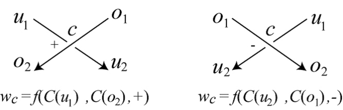
Let $W_{f}(D,C)$ be the sum of the weights for all the real-crossings of $D$, that is,

We denote by $\Phi_{f}(D)$ the multi-set

Theorem 1.3 implies that the multi-set $\Phi_{f}(D)$ is useful to detect the necessity of RII-moves.

xProof of Theorem 1.3. Let $D$ and $D^{\prime}$ be virtual-knot diagrams such that $D^{\prime}$ is obtained from $D$ by a single RI-move. For an $n$-up-down coloring $C$ of $D$, we set an $n$-up-down coloring $C^{\prime}$ of $D^{\prime}$ so that $C$ is corresponding to $C^{\prime}$ by the bijection defined in the proof of Theorem 1.1. Then as shown in Figure 13, we have

for some $a\in\mathbb{Z}_{n}$ and $\varepsilon\in\{+,-\}$. By the condition (0) of an $n$-up-down cocycle, since $f(a,a,\varepsilon)=0$, $W_{f}(D,C)=W_{f}(D^{\prime},C^{\prime})$ holds.

Next let us consider the cases of RIII-moves. As shown in Figure 14, we have eight RIII-moves (1)-(8). Let $D$ and $D^{\prime}$ be virtual-knot diagrams such that $D^{\prime}$ is obtained from $D$ by the RIII-move (1) in Figure 14. For an $n$-up-down coloring $C$ of $D$, we set an $n$-up-down coloring $C^{\prime}$ of $D^{\prime}$ so that $C$ is corresponding to $C^{\prime}$ by the bijection defined in the proof of Theorem 1.1. Then we have

for some $a,b,c\in\mathbb{Z}_{n}$, see Figure 14. By the condition (1) of an $n$-up-down cocycle, since the right side of the above equation is equal to $0$, we have $W_{f}(D,C)=W_{f}(D^{\prime},C^{\prime})$. Similarly, in the cases of the other RIII-moves (2)-(8), by the conditions (2)-(8) of an $n$-up-down cocycle, respectively, we have $W_{f}(D,C)=W_{f}(D^{\prime},C^{\prime})$.

It is obvious that the other generalized Reidemeister moves other than the RII-moves also do not change the weight sum $W_{f}(D,C)$, see Figure 15 for the VRIV-moves.

As a consequence, we have a bijection $\Phi_{f}(D)\to\Phi_{f}(D^{\prime}),W_{f}(D,C)\mapsto W_{f}(D^{\prime},C^{\prime})$ such that $W_{f}(D,C)=W_{f}(D^{\prime},C^{\prime})$ for each of the generalized Reidemeister moves other than the RII-moves. ∎

x

Now we assume that the $n$-up-down cocycle $f$ is shiftable. Then the value $W_{f}(D,C)$ does not depend on the choice of the $n$-up-down coloring $C$, see Figure 9 and Corollary 3.5.

Hence, we denote by $\Phi_{f}^{\rm shift}(D)$ the value $W_{f}(D,C)$ for some $n$-up-down coloring $C$. Note that $\Phi_{f}(D)$ and $\Phi_{f}^{\rm shift}(D)$ are essentially the same. Next property is obtained as a corollary of Theorem 1.3.

xProof of Theorem 1.4 Let $D^{\prime}$ be a virtual-knot diagram which is obtained by taking the connected sum $\Delta\sharp D$ depicted in Figure 12, where we may replace the diagram $\Delta$ with the one obtained after performing a single RI-move as shown in the lower picture of Figure 12. Then $D$ and $D^{\prime}$ represent the same virtual-knot.

By Lemma 4.6 and Example 4.7, we have

Therefore by Corollary 4.5, at least one RII-move is needed to transform $D$ to $D^{\prime}$. ∎

x

• 1.

  (To study about a generalization of up-down colorings.)

Let $n$ be a nonnegative integer and $P$ and $N$ integers.

An $(n;P,N)$-up-down coloring of a virtual-link diagram $D$ is a map $C:\mathcal{SA}(D)\to\mathbb{Z}_{n}$ satisfying the following conditions: For a real-crossing $c$ of $D$, let $u_{1}$, $u_{2}$ (resp. $o_{1}$, $o_{2}$) be the under-semi-arcs (resp. over-semi-arcs) around $c$ such that the orientation of $D$ points from $u_{1}$ to $u_{2}$ (resp. from $o_{1}$ to $o_{2}$). Then

• •

  if $c$ is positive,

  $\displaystyle C(u_{2})=C(u_{1})-P\mbox{\ and \ }C(o_{2})=C(o_{1})+P,$

  and

• •

  if $c$ is negative,

  $\displaystyle C(u_{2})=C(u_{1})-N\mbox{\ and \ }C(o_{2})=C(o_{1})+N.$

It is easily seen that $(n;P,N)$-up-down colorings are a generalization of up-down colorings. Moreover the numbers of $(n;P,N)$-up-down colorings of virtual-link diagrams can be used to detect the necessity of RII-moves. In addition, the argument in Section 4 is also extended in the cases using $(n;P,N)$-up-down colorings. We aim to address these topics including some applications in future work. (Moreover note that an $(n;P,N)$-up-down coloring is a biquandle coloring if and only if $P=-N$.)

• 2.

  (To find a (co)homology theory related to up-down cocycles.)

In [2], a quandle cohomology theory was introduced, see also [4, 5]. The $2$- or $3$-cocycles (or $3$- or $4$-cocycles) are used to define a quandle cocycle invariant of an oriented classical-link (or an oriented surface-link). The cocycle conditions are related to the RI-moves and an RIII-move, see [2].

In Section 4, we defined an up-down cocycle. The cocycle conditions are also related to the RI-moves and all the RIII-moves. However we do not know if there exists a (co)homology theory which are related to up-down cocycles. Hence, it might be natural to ask the following question:

• 3.

  (To find an application for classical-knots.)

In Section 4, by our method, we found two trivial virtual-knot diagrams such that at least one RII-move is needed for transformations between them. For classical-knot diagrams, we give the following question:

• 4.

  (To study about the other generalized Reidemeister moves.)

When we restrict the moves $\mathcal{M}$ to $\mathcal{M}\in\{RI,RI\hskip-1.5ptI,RI\hskip-1.5ptI\hskip-1.5ptI,VRI\}$, the statement of the above question is true, see [3, 6, 12, 13, 16]. Note that it is easy to construct a pair of trivial virtual-knot diagrams which need at least one VRI-move between them, since the parity of the number of virtual-crossings is unchanged under the generalized Reidemeister moves except for the VRI-move. If we find such a pair of trivial virtual-knot diagrams for the other generalized Reidemeister moves, we might be able to answer the next conjecture:

References

- [1] J. S. Carter, M. Elhamdadi, M. Saito and S. Satoh: A lower bound for the number of Reidemeister moves of type III, Topology and its Applications 153 (2006), 2788–2794.
- [2] J. S. Carter, D. Jelsovsky, S. Kamada, L. Langford and M. Saito: Quandle cohomology and state-sum invariants of knotted curves and surfaces, Trans. Amer. Math. Soc. 355 (2003), no. 10, 3947–3989.
- [3] Z. Cheng and H. Gao: A note on the independence of Reidemeister moves, J. Knot Theory Ramifications 21 (2012), no. 9, 1220001, 7 pp.
- [4] R. Fenn, C. Rourke and B. Sanderson: Trunks and classifying spaces, Appl. Categ. Structures 3 (1995), no. 4, 321–356.
- [5] R. Fenn, C. Rourke and B. Sanderson: James bundles and applications, preprint (1996), http://www.maths.warwick.ac.uk/~cpr/ftp/james.ps.
- [6] T. J. Hagge: Every Reidemeister move is needed for each knot type, Proc. Amer. Math. Soc. 134 (2005), 295–301.
- [7] J. Hass and T. Nowik: Invariants of knot diagrams, Math. Ann. 342 (2008), 125–137.
- [8] C. Hayashi: A lower bound for the number of Reidemeister moves for unknotting, J. Knot Theory Ramifications 15 (2006), 313–325.
- [9] C. Hayashi, M. Hayashi and T.Nowik: Unknotting number and number of Reidemeister moves needed for unknotting, Topology and its Applications 159 (2012), 1467–1474.
- [10] L. H. Kauffman: Virtual knot theory, European J. Combin. 20 (1999), 663–690.
- [11] A. M. Lowrance: Alternating distance of knots and links, Topology and its applications 182 (2015), 53–70.
- [12] V. O. Manturov: Knot Theory, Chapman & Hall/CRC, Boca Raton, FL (2004), xiv+400 pp.
- [13] O. P. Östlund: Invariants of knot diagrams and relations among Reidemeister moves, J. Knot Theory Ramifications 10 (2001), 1215–1227.
- [14] K. Reidemeister: Elementare Begrndung der Knotentheorie, Abh. Math. Sem. Univ. Hamburg. 5 (1927) 24–32.
- [15] A. Shimizu: The warping polynomial of a knot diagram, J. Knot Theory Ramifications 21 (2012), 1250124, 15 pp.
- [16] B. Trace: On the Reidemeister moves of a classical knot, Proc. Amer. Math. Soc. 89 (1983), 722-724.