Towards Computing the Margin of Victory in STV Elections
Abstract
The Single Transferable Vote (STV) is a system of preferential voting employed in multi-seat elections. Each vote cast by a voter is a (potentially partial) ranking over a set of candidates. No techniques currently exist for computing the margin of victory (MOV) in STV elections. The MOV is the smallest number of vote manipulations (changes, additions, and deletions) required to bring about a change in the set of elected candidates. Knowledge of the MOV of an election gives greater insight into both how much time and money should be spent on the auditing of the election, and whether uncovered mistakes (such as ballot box losses) throw the election result into doubt—requiring a costly repeat election—or can be safely ignored. In this paper, we present algorithms for computing lower and upper bounds on the MOV in STV elections. In small instances, these algorithms are able to compute exact margins.
1 Introduction
The Single Transferable Vote (STV) is a system of preferential voting employed in multi-seat elections. It is used to elect candidates to the Australian Senate, in all elections in Malta, and in most elections in the Republic of Ireland (Farrell and McAllister, 2005). No techniques currently exist for computing the smallest number of vote manipulations (changes, additions, and deletions) required to bring about a change in the set of elected candidates—the margin of victory (MOV). The ability to compute this margin has significant value. In the 2013 election of six candidates to Western Australia’s Senate a discrepancy of 1,375 initially verified votes was discovered during a recount. The election result was overturned, and a repeat election held in 2014. If the MOV for the original election was known, the question of whether the loss of these votes may have altered the resulting outcome could have been answered. In this instance, if the MOV was greater than 1,375 votes, the inclusion of these 1,375 lost votes would not have changed the election outcome.
In an STV election, each vote is a (potentially partial) ranking over a set of candidates. For example, in an election with candidates and a vote [ ] expresses a first preference for candidate , a second for and a third for . At the start of the counting process, each vote is initially awarded to its highest ranked candidate. In the above vote, is the highest ranked candidate. The votes awarded to each candidate forms their tally. Candidates whose tallies exceed (or reach) a quota, defined in terms of the number of seats to be filled and votes cast in the election, are elected to a seat. As each candidate is elected, their surplus (the number of votes by which their tally exceeds the quota) is computed, and a subset of their votes (with a combined value equal to the surplus) is distributed to their next preferred candidate (in the above vote, the next preferred candidate after is ). Where multiple candidates have a quota’s worth of votes in their tally, the candidate with the largest surplus is elected first, and their surplus is distributed. Then, if there are still seats to fill, the candidate with the next largest surplus is elected, and their surplus distributed (and so on). If no remaining candidate has a quota’s worth of votes, and one or more seats remain empty, the candidate with the fewest votes is eliminated and their votes distributed to their next preferred candidates. If the number of candidates remaining (unelected and not yet eliminated) equals the number of seats left to be filled, these candidates are elected and the STV counting process terminates.
Several STV variants exist, differing in the way that surpluses are distributed (Weeks, 2011). Consider a candidate with a tally of 100 votes and a surplus of 40 votes. The Inclusive Gregory Method redistributes all 100 votes, each with an assigned value of 0.4 (each vote is worth 0.4 votes), to their next highest ranked candidate that is ‘still standing’ (has not yet been elected or eliminated) (Miragliotta, 2004). In the STV variant we consider in this paper, candidates whose tallies have reached or exceeded the quota (but have not yet been awarded a seat) receive no further votes from the surplus distributions of other candidates.
Computing the MOV of an STV election is an extremely complex combinatorial optimisation problem. In an election with candidates, and available seats, there are possible allocations of candidates to these seats, and different orders in which candidates can appear in the elimination and election sequence. Our task is to find an election outcome, out of the possibilities, that differs from the original outcome of the election and that requires the least number of vote manipulations to realise.
We develop, in this paper, an algorithm for computing exact margins of victory in STV elections that use the Inclusive Gregory Method of surplus distribution—arguably the simplest and most straightforward of the existing variants. In Section 2, we step through the counting process that takes place in STV elections, under the Inclusive Gregory Method, in two example STV instances. The algorithm we present in this paper (labelled margin-stv) is an adaptation of existing work for computing margins in Instant Runoff Voting (IRV) elections (Blom et al., 2016). IRV is a single-seat variant of STV and is employed in lower house elections across Australia, in which a single candidate is elected to a single seat. In an IRV election, candidates with the fewest votes are eliminated, and their votes redistributed to later ranked candidates, until a candidate attains a majority of the available votes, and is declared the winner. The computation of exact IRV and STV victory margins is known to be NP-hard (Bartholdi III and Orlin, 1991; Conitzer et al., 2007; Xia, 2012; Rothe and Schend, 2013; Narodytska and Walsh, 2014).
Our margin-stv algorithm represents the outcome of an STV election as a sequence of candidate elections and eliminations (e.g., elected, eliminated, eliminated, elected). We present a mixed-integer non-linear program (MINLP) that, given such an outcome, and the set of votes cast in the election, computes the smallest number of vote manipulations required to realise the outcome. A vote manipulation replaces the ranking of a vote (e.g., [ ]) with an alternate ranking (e.g., [ ]). Consider an election over candidates , in which candidates are elected to a seat. Our margin-stv algorithm applies branch-and-bound to search the space of alternate election outcomes (in which the set of winning candidates ) for one that requires the least number of vote manipulations to realise. We show that margin-stv is able to compute exact margins in some small STV election instances. We develop a relaxation of this algorithm capable of computing lower bounds on the margin of victory in larger, more realistic STV election instances.
The remainder of this paper is structured as follows. Section 2 describes the STV counting algorithm. Preliminary definitions and concepts required in the explanation of our margin-stv algorithm are presented in Section 3. Related work is discussed in Section 4. Mechanisms for computing simple upper bounds on the degree of manipulation required to alter the outcome of an STV election are presented in Section 5. Section 6 presents our MINLP for computing the smallest degree of manipulation required to realise a specific election outcome (a specific sequence of elections and eliminations). A rule for computing a lower bound on this degree of manipulation is presented in Section 7. Using these upper and lower bounding techniques as building blocks, we present our margin-stv algorithm, and a relaxed variant of this algorithm, in Section 8. We evaluate these algorithms on a range of both small and large STV election instances in Section 9.
2 The Single Transferable Vote (STV)
This section describes the STV vote counting algorithm that we consider in this paper, outlined in Figure 1. We illustrate this algorithm in the example election shown in Table 1. In Step 1 of the counting algorithm the quota of the election is calculated, according to Equation 1. This is known as the Droop quota, and represents a threshold that each candidate must reach before they are elected to a seat. In the election of Table 1 there are 2 seats to be filled and 60 cast votes. The quota in this election is 21 votes.
| (1) |
Each vote cast in the election starts with a value of 1. The total value of the votes a candidate has in their tally is computed as shown in Equation 2. As the STV algorithm proceeds, votes will move from the tally of one candidate to that of others. The value of these votes—the extent to which they contribute to a candidate’s tally value—will change over the course of the algorithm.
| (2) |
Each vote is assigned to its first ranked candidate (Step 2). The first ranked candidate of vote [ ] is . The total value of the votes in each candidate’s tally is computed. Table 1(b) shows that the tally values of candidates to after this first round of counting are 26, 10, 9, and 15. The candidates whose tally value equals or exceeds the quota are placed in a list sorted in decreasing order of surplus size. A candidate’s surplus is equal to the difference between their tally value and the quota, as shown in Equation 3. In our example, is the only candidate whose tally has exceeded the quota with a surplus of 5 votes.
| (3) |
If this list of candidates with a surplus (denoted surpluses in Figure 1) is not empty, we select the first candidate in this list, and elect them to a seat (Step 9). If we have filled all available seats, the algorithm terminates (Step 10). Otherwise, we redistribute the votes in ’s tally. Each vote is placed in the tally of the next most preferred eligible candidate after in its ranking. Candidates that have been elected, eliminated, or whose tally value equals or exceeds the quota are not eligible. The set of votes in ’s tally that have no eligible next preferred candidate are exhausted (not redistributed). The remainder are labelled transferable (Step 11). These votes will have a reduced value when they are redistributed. Their current value is reduced by a factor known as the transfer value, computed (in Step 12) as shown in Equation 4.
| (4) |
| Ranking | Count |
|---|---|
| [, ] | 4 |
| [] | 20 |
| [, ] | 9 |
| [, , ] | 6 |
| [, , ] | 15 |
| [, ] | 6 |
| Seats: 2 | |||
|---|---|---|---|
| Quota: 21 | |||
| Candidate | Round 1 | Round 2 | Round 3 |
| elected | eliminated | elected | |
| 26 | — | — | |
| 10 | 10 | — | |
| 9 | 14 | 24 | |
| 15 | 15 | 15 |
Consider our example in Table 1. Candidate is elected to a seat, and has 6 transferable votes with ranking [ ]. The remaining votes in ’s tally have a ranking of []. These votes have no eligible next preference and are exhausted (not redistributed). The transfer value assigned to ’s transferable votes is 0.83. All 6 votes with ranking [ ] are given to candidate , but they now have a combined value of 5.
| 1 | Compute the Quota for the election (Equation 1) | |||
| 2 | Assign votes to their first ranked candidates (each vote has a value of ) | |||
| 3 | While a seat remains to be filled do | |||
| 4 | Let surpluses denote the candidates whose tally equals or | |||
| exceeds the quota (in order of decreasing surplus size) | ||||
| 5 | If the surpluses set is empty then | |||
| 6 | Eliminate a candidate , of those remaining, with the smallest tally | |||
| 7 | Redistribute each vote in ’s tally to its next preferred candidate at its current value | |||
| 8 | Else | |||
| 9 | Elect the first candidate in surpluses, , to a seat | |||
| 10 | if all seats are filled then stop | |||
| 11 | Compute the number of transferable votes in ’s tally | |||
| 12 | Compute the transfer value of these transferable votes | |||
| 13 | Redistribute each transferable vote in ’s tally with a value of , where | |||
| is its current value, to its next preferred candidate (skipping over candidates | ||||
| that have been elected, eliminated, or are in the surpluses set) | ||||
| 14 | If the number of unfilled seats and remaining candidates are equal then | |||
| 15 | Elect all remaining candidates to a seat |
If, in Step 4, no candidate has a tally value that equals or exceeds the quota, the candidate with the smallest tally value is eliminated (Step 6). The votes in their tally are redistributed to later preferences. The votes in ’s tally that have as a first preference will have a value of 1 (as a consequence of Step 2). Votes that has received after prior surplus distributions will have a reduced value. All votes in ’s tally that have an eligible next preferred candidate (a candidate that is still standing) are given to that candidate at their current value (Step 7). If the contribution to ’s tally value of a vote is , then that vote’s contribution to its next preferred candidate’s tally is also . Consider again the example of Table 1. After the election of candidate and the redistribution of their votes, candidates to have tally values of 10, 14, and 15. No candidate has a quota of votes in their tally. Candidate has the smallest tally value, and is eliminated. Each of ’s votes—four with ranking [ ] and 6 with ranking [ ]—still have a value of 1 and are redistributed to candidate . Candidates and now have tally values of 24 and 15.
After a candidate has been elected or eliminated, we check whether the number of unfilled seats and the number of remaining candidates (that have not yet been elected or eliminated) are equal (Step 14). If so, all remaining candidates are elected to a seat irrespective of their tally value (Step 15). If not, the total value of the votes in each remaining candidate’s tally is recomputed and we return to Step 4. In the example of Table 1, the algorithm recomputes the tally values of candidates and in Step 4, and places in the surpluses list. Candidate is elected to the final seat, and the algorithm terminates in Step 10. The STV algorithm proceeds in rounds that consist of: computing the total value of each candidate’s tally; electing the candidate with the largest surplus (if such a candidate exists) and redistributing their votes; or eliminating the candidate with the smallest tally value (if no candidate has a quota) and redistributing their votes.
Let us consider a second example STV election, shown in Table 2. Candidates , , , and have initial tallies of 31, 17, 5, and 10 votes. The quota for the election is 22, and is placed into the list of candidates with a surplus in Step 4. Candidate is elected to the first of two available seats in Step 9, and has 13 transferable votes in their tally (Step 11). The transfer value to be applied to those votes is 0.69 (its surplus of 9 divided by the number of transferable votes 13). In Step 13, candidate is given 5 votes of ranking [ ], with the total value of these votes equal to 3.46. Candidate is given 8 votes of ranking [ ], with the total value of these votes equal to 5.54. In the second round of counting, now has a total tally value of 20.46 votes and a total tally value of 15.54. No candidate has a quota, and candidate , with the smallest tally, is eliminated (in Step 6). Candidate is given 5 votes with ranking [ ]. In the next round of counting, candidate has exceeded a quota and is elected to the last seat (Step 9).
| Ranking | Count |
|---|---|
| [, , ] | 5 |
| [] | 18 |
| [, ] | 10 |
| [, , ] | 5 |
| [, , ] | 17 |
| [, , , ] | 8 |
| Seats: 2 | |||
|---|---|---|---|
| Quota: 22 | |||
| Candidate | Round 1 | Round 2 | Round 3 |
| elected | eliminated | elected | |
| 31 | — | — | |
| 17 | 20.46 | 25.46 | |
| 5 | 5 | — | |
| 10 | 15.54 | 15.54 |
In many STV variants, the last bundle of votes received by a candidate, at any point in the counting process, is known as their last parcel. In the Original Gregory Method, votes in an elected candidate’s last parcel (and no others) are transferred (at a fraction of their value) during surplus distribution. The total value of the votes transferred is equal to the candidate’s surplus. Some jurisdictions do not assign fractional values to distributed votes, but transfer a random selection of votes from a candidate’s last parcel at their full value, the total of which equals the candidate’s surplus. Much of the complexities involved in vote distribution across these variants are in place to support easier and faster manual vote counting. Weeks (2011) and Miragliotta (2004) provide a good summary of the range of STV variants used in practice.
3 Preliminaries
Definition 1 formally defines an STV election . Our representation of the outcome of an STV election—as a sequence of candidate elections and eliminations—is outlined in Definition 2. The margin of victory (MOV) of an STV election is defined in Definition 3. The primary vote of a candidate is computed as described in Definition 4, and used to compute simple upper bounds on the MOV of an STV election in Section 5.
Definition 1.
STV Election () An STV election is defined as a tuple where is a set of candidates, the set of votes cast in the election, the election quota (the number of votes a candidate must attain to be elected to a seat, as defined in Equation 1), the number of seats to be filled, and the set of candidates elected to a seat (according to the counting algorithm outlined in Figure 1). Each vote is a partial or complete ranking over (e.g., the vote , in an election with candidates , expresses a first preference for candidate , a second for , and a third for ).
Definition 2.
Election Order () Given an STV election , we represent the outcome of the election as an election order —a sequence of tuples where and . The tuple indicates that candidate is elected to a seat, and that is eliminated. An election order defines the sequence of elections and eliminations that arise as the STV counting algorithm (Figure 1) is executed. The order , for example, indicates that candidate is elected to a seat in the first round of counting, followed by the elimination of candidates and , and the election of .
Definition 3.
Margin of Victory (MOV) The margin of victory for an STV election is defined as the smallest number of vote manipulations required to ensure that a set of candidates are elected to a seat (i.e., at least one candidate in must not appear in ). A single manipulation changes the ranking on a single vote to an alternate ranking. For example, consider a vote with ranking [ ]. Replacing ’s ranking with the alternate ranking [ ] represents a single manipulation.
Definition 4.
Primary Vote The primary vote of a candidate in an STV election is defined as the total number of votes in in which is ranked highest (i.e., is ranked first). For example, the vote contributes to the primary vote of candidate .
4 Related Work
The computation of victory margins in both STV and Instant Runoff Voting (IRV) elections is NP-hard (Bartholdi III and Orlin, 1991; Conitzer et al., 2003; Conitzer et al., 2007; Xia, 2012; Rothe and Schend, 2013; Narodytska and Walsh, 2014). To the best of our knowledge, the algorithms presented in this paper form the first attempt to compute margins in STV elections. Blom et al. (2016) present a branch-and-bound algorithm for computing victory margins in IRV elections, itself an adaptation of earlier work by Magrino et al. (2011). An IRV election elects a single winner from a field of candidates on the basis of the votes cast in the election. As in an STV election, each vote is a (possibly partial) ordering over the candidates in . An IRV election proceeds in rounds of candidate elimination. Each vote is placed in the tally of the candidate that appears first in its ordering. In the first round, the candidate with the least votes in their tally is eliminated. Each of these votes is placed in the tally of its next preferred candidate. Votes with no next preferred candidate become exhausted (are not redistributed). This process of candidate elimination is repeated until only a single candidate remains—this candidate is the winner of the election. Unlike IRV, STV elects multiple candidates with the counting algorithm alternating between rounds of candidate election and candidate elimination. The votes in the tallies of elected candidates are redistributed at a reduced value.
Magrino et al. (2011) represent the outcome of an IRV election as a candidate sequence with candidates listed in the order in which they are eliminated (with the last candidate being the winner). Given such a sequence , and a collection of votes, a linear program (LP) is presented that computes the smallest number of vote manipulations required to realise . This linear program is labelled DistanceTo. In an election with winner , Magrino et al. (2011) search the space of alternate elimination sequences (in which a candidate other than is elected) for one requiring the least number of vote manipulations to realise. A key observation made by Magrino et al. (2011) is that, given a partial sequence of candidates , the DistanceTo LP computes a lower bound on the number of vote manipulations required to realise any elimination order that ends in . Magrino et al. (2011) progressively explore and build partial candidate elimination orders in a branch-and-bound algorithm. The last round margin (LRM) of the election (defined as the difference in the tallies of the winning candidate and runner-up, divided by two and rounded up) is used as an upper bound on the MOV. Consider an IRV election with candidates , , , and , with outcome [ ], where is the winning candidate. Partial orders containing a single candidate (not including the original winner ) are added to a tree. DistanceTo is applied to each partial order in this tree to compute a lower bound on the number of vote manipulations required to realise an elimination sequence ending in . The partial order with the smallest DistanceTo evaluation is expanded by adding a candidate (not already in ) to the start of the sequence. Partial orders with evaluations equal to or larger than the current upper bound are pruned. When a complete elimination order (involving all candidates) is formed, its DistanceTo evaluation is used to revise the current recorded upper bound. The algorithm terminates once all partial orders have either been expanded or pruned, with the revised upper bound returned as the MOV.
Blom et al. (2016) improve the efficiency of the branch-and-bound algorithm of Magrino et al. (2011) by introducing new rules for computing lower bounds on the manipulation required to realise each partial order in the search tree. These rules typically result in tighter (i.e., higher) lower bounds for each partial order than supplied by solving the DistanceTo LP. Consequently, Blom et al. (2016) are able to: prune larger portions of the space of partial elimination sequences; reduce the number of calls to the DistanceTo LP; and quickly compute margins in elections for which the algorithm of Magrino et al. (2011) times out after 72 hours of computation. Our margin-stv algorithm shares a similar structure to that of Blom et al. (2016) and Magrino et al. (2011), in that it searches the space of alternate election and elimination sequences using branch-and-bound. The margin-stv algorithm differs in several key aspects: each node is a partial sequence of candidate elections and eliminations (in place of a sequence of eliminations); a MINLP (in place of an LP) is used to evaluate nodes in this search tree; and the descendants of a partial sequence are all complete sequences that start with (in place of all sequences than end in ). Moreover, a variation of the winner elimination upper bound for IRV elections (Cary, 2011) is used as an initial upper bound on the STV MOV (as described by Chilingirian et al. (2016)). Section 8 describes the margin-stv algorithm in detail.
The winner elimination upper bound (on the IRV margin of victory) of Cary (2011) finds the most efficient way to eliminate the apparent winner of an IRV election at each elimination round, returning the least-cost (involving the smallest number of vote changes) of these. Chilingirian et al. (2016) develop a version of this upper bound for use in STV elections. Figure 2 outlines this STV variant of the winner elimination upper bound. Consider the example STV election of Table 1, where was elected in the first round of counting, eliminated in the second, and elected in the third (at which point both available seats had been filled). Following the algorithm listed in Figure 2, the winner elimination upper bound () is initially set to the total number of votes cast in the election (Step 1), which is 60. The set of candidates that are (eventually) elected is { }. In the first round of counting, a candidate () is elected. The algorithm moves on to the second round (Step 3), in which a candidate () is eliminated with 10 votes ( in Step 6). In Step 7, we consider each candidate in that has not been elected by round 2—candidate —and determine how they could be eliminated in this round. Candidate has 14 votes in round 2 ( in Step 8). We could certainly eliminate by taking 4 votes from their tally ( in Step 9) and giving them to some other candidate (, for example). However, candidate can still be eliminated in this round if we take 2 votes from their tally and give them to (Steps 11 and 12), under the assumption that we can break the resulting tie between and in ’s favour. The winner elimination upper bound is set to 2 in Step 12. The algorithm moves on to the last round of counting in which no candidate is eliminated. Steps 5 to 12 are skipped and a winner elimination upper bound of 2 is returned.
| 1 | ||||
| 2 candidates (eventually) elected | ||||
| 3 for each round of counting do | ||||
| 4 | if a candidate is eliminated in round do | |||
| 5 | candidate eliminated in round | |||
| 6 | number of votes in ’s tally in round | |||
| 7 | for each that has not yet been elected by round do | |||
| 8 | number of votes in ’s tally in round | |||
| 9 | ||||
| 10 | ||||
| 11 | if is less than or equal to tallies of all candidates still standing (excluding ) do | |||
| 12 | ||||
| 13 return |
To the best of the authors knowledge, the work of Chilingirian et al. (2016) describes the only attempt to compute bounds on the MOV for STV elections (in its adaptation of the winner elimination upper bound of Cary (2011)). The algorithms we present in this paper are, to the best of our knowledge, the first attempts to compute exact margins in small STV elections and lower bounds on the MOV in larger instances. IRV elections, in contrast, have received more consideration. Blom et al. (2016) and Magrino et al. (2011) present algorithms for computing exact margins in IRV elections. A number of works have presented algorithms for computing lower and upper bounds on IRV margins (see Cary (2011) and Sarwate et al. (2013)).
The focus of this paper is the computation of the MOV for STV elections. This MOV is defined as the smallest number of vote manipulations (the replacing of the ranking of a vote with an alternate ranking) required to ensure that a different set of candidates is elected (i.e., at least one candidate in this set is replaced with one that was not originally elected to a seat). Similar questions have been considered for alternate voting rules. The complexity of manipulating an election with bribery is considered by Faliszewski et al. (2009), under a number of voting schemes: Condorcet-based; approval voting; scoring rules; veto rules; and plurality. Their aim is to find a manipulation to achieve a desired election result, while minimising the cost of bribes given to voters for changing their vote. If the cost of bribing a voter to change their vote is 1, this least cost set of bribes is equivalent to the margin of victory, as we have defined it. Kaczmarczyk and Faliszewski (2016) consider a variant of the bribery problem (destructive shift bribery) in which voters can be bribed to demote the position of a candidate in their ranking by positions (i.e., to move a candidate down in their ranking by positions) in a bid to ensure that does not win the election. The authors analyse the complexity of destructive shift bribery for a number of voting rules (-Approval, Borda, Copeland and Maximin). Polynomial-time algorithms are presented for computing the smallest set of desired bribes in the case of the k-Approval, Borda, and Maximin rules, while the problem is shown to be NP-complete for the Copeland rule. Schürmann (2017) describe a model-checking-based approach for the computation of margins in D’Hondt elections, applying their approach to the 2015 Danish national parliamentary elections. The STV elections we consider in this paper vary considerably from the voting rules considered by Kaczmarczyk and Faliszewski (2016), and Schürmann (2017). We refer the reader to Brandt et al. (2016) for further discussion on bribery and manipulation problems in the computational social choice context.
Given an STV election , our margin-stv algorithm relies on: a mechanism for computing an upper bound on the manipulation required to change the outcome of ; a mechanism for computing the smallest manipulation required to realise a specific outcome for —a specific sequence of candidate eliminations and elections ; and a mechanism for computing a lower bound on the degree of manipulation required to realise a candidate order that starts with a partial sequence of elections and eliminations . These mechanisms are provided in Sections 5 to 7, and form the basis of our branch-and-bound algorithm.
5 Simple Upper Bounds on the STV MOV
Figure 2 presents an algorithm for computing an upper bound (a winner elimination upper bound) on the STV MOV11 1 This algorithm has been extracted from the work of Chilingirian et al. (2016). The algorithm is not explicitly presented in that paper, but can be found in code, implemented by Andrew Conway, for analysing the 2012 local government elections in New South Wales, Australia. This code is available at: https:/github.com/SiliconEconometrics/PublicService. In elections where all seats are filled by a candidate prior to any eliminations taking place (e.g., an election with 2 seats, 4 candidates, and outcome [ ]), this algorithm is not able to reduce the upper bound from its original value (the total number of votes cast in the election). In these instances, we introduce a simple bound on the STV MOV, computed as follows. Consider an election . The STV counting algorithm of Figure 1 elects candidates to a seat once the number of votes in their tally reaches or exceeds . To change the outcome of , with winning candidates , we must find a series of vote manipulations that elects a candidate to a seat. It is clear that we can elect , with primary vote (the total number of votes in in which is ranked first), if we take votes away from other candidates and give them to (we replace the ranking of these votes by a ranking that preferences first). We compute for each and take the smallest result as an upper bound on the STV MOV. We call this bound the Simple-STV upper bound.
6 Computing Minimal Manipulations: A MINLP
Given an IRV election and a sequence of candidate eliminations , Magrino et al. (2011) present a linear program (LP) for computing the smallest number of vote manipulations required to ensure candidates are eliminated in the order specified in . In this section, we present a mixed-integer non-linear program (MINLP) that, given an STV election , and a candidate order (a sequence of candidate elections and eliminations), computes the smallest number of vote manipulations (changes to votes in ) required to realise . We re-use some notation and constraints introduced in the LP of Magrino et al. (2011). The votes in form the original profile of the election. The MINLP below, denoted DistanceToSTV, introduces variables indicating which votes in are to be changed, and what their ranking will be in a new or modified profile. The constraints of the following MINLP are designed to enforce a specific candidate order by modifying the smallest number of votes in (where required).
6.1 Notation
Sets and Indices
| A signature is a partial or total ranking over the candidates in ; is the set of all possible partial or total rankings over (including those that do not appear on a vote in ). | |
| The set of rounds of counting in the election—in each round a candidate is either elected to a seat or eliminated. | |
| The subset of vote signatures that could possibly be in the tally of candidate at the start of round (this can be inferred on the basis of the order of candidates in ). | |
| The candidate that is elected or eliminated in round (according to ). | |
| The set of candidates that appear before candidate in the preference ordering of signature that are still standing (have not been elected or eliminated) at the end of round . | |
| The set of candidates still standing at the start of round . | |
| The subset of candidates in that are elected to a seat according to . | |
| The subset of candidates in that are eliminated according to . |
Constants
| Number of votes with signature cast in election (i.e., the number of votes in whose ranking matches signature ). | |
| Known upper bound on the number of vote manipulations required to realise (such as the winner elimination upper bound of Figure 2 or the Simple-STV upper bound of Section 5). |
Decision Variables
| Integer number of votes in that are modified so that their new signature is . | |
| Integer number of votes whose signature in (the original profile) is , but are modified to something other than in the new profile. | |
| Integer number of votes with signature in the new election profile. | |
| Transfer value of votes being redistributed from an elected candidate in round . | |
| Number of votes eligible for transfer, from the candidate elected to a seat in round , to candidates that are still standing at the end of round . | |
| Binary variable with a value of 1 if the tally of candidate exceeds or equals the quota at the start of round , and 0 otherwise. | |
| Floating point number of votes in the tally of candidate at the start of round . | |
| Floating point number of votes with signature in the tally of candidate at the start of round . | |
| Floating point number of votes with signature transferred to candidate from the candidate elected or eliminated in round . |
6.2 Objective
The objective of DistanceToSTV is to minimise the number of votes in whose signature is changed.
| (5) |
6.3 Constraints
Constraints (6) and (7) appear in the LP of Magrino et al. (2011). Constraint (6) ensures that the total number of votes in the new election profile (after manipulation) is equal to the total number of votes in the original profile. This assumption is made by both Blom et al. (2016) and Magrino et al. (2011). Blom et al. (2016) explore variations of the DistanceTo LP of Magrino et al. (2011) in which this constraint is removed, and a manipulation may add votes (for example, arising from voters voting multiple times), or remove votes (for example, arising from ballot box losses). We intend, in future work, to consider the ‘deletion-only’ and ‘addition-only’ settings analysed by Blom et al. (2016) for IRV elections, in the STV setting. Constraint (7) defines the number of votes with signature in the new profile, .
| (6) | ||||||
| (7) | ||||||
Constraint (8) ensures that candidates who have achieved a quota by round , have also achieved a quota by round . Constraints (9) and (10) ensure that that number of votes a candidate has in their tally at the start of round is greater than or equal to if has achieved a quota by round ( is 1) and less than otherwise ( is 0, and ).
| (8) | ||||||
| (9) | ||||||
| (10) |
Constraints (11) and (12) define the number of votes of signature in candidate ’s tally at the start of round . Where , this is equal to the number of votes of signature in candidate ’s tally at the start of the previous round, plus the number of votes of signature distributed to from the candidate elected (or eliminated) in round . As all votes of a single signature will reside in the tally of only one candidate at any point in time, at least one of and will be zero in each instance of Constraint (12). Although the order in which candidates are elected and eliminated is fixed (to that defined by ), the round in which a candidate is given, via distribution, votes of certain signatures can vary. Consider a candidate whose tally has reached or exceeded the quota in round . Candidate may have to wait several rounds to be elected to a seat, if one or more other candidates have also reached a quota by round , and have more votes in their tallies (they are elected before ). While candidate is waiting to be elected, they are not given any additional votes during the distribution of the surpluses of elected candidates—these votes skip and are given to the next eligible candidate in their ranking. As the candidate order does not prescribe exactly when an elected candidate achieves a quota, we must support the possibility that votes of certain signatures can be distributed to a candidate in one of a number of different rounds. Constraint (13) sums the total number of votes for candidate at the start of round .
| (11) | ||||||
| (12) | ||||||
| (13) |
Constraint (14) ensures that the candidate elected to a seat in round has more (or an equal number of) votes in their tally at the start of round than all other candidates who are still standing (have not been eliminated or elected before round ). Conversely, a candidate who is eliminated in round must have fewer (or an equal number of) votes in their tally at the start of round than all other candidates who are still standing (Constraint (15)). Moreover, a candidate can only be eliminated in a round if no other remaining candidate has a quota’s worth of votes in their tally at the start of the round (Constraint (16)).
| (14) | ||||||
| (15) | ||||||
| (16) |
Constraint (17) defines the value of variable (the total number of votes of signature distributed to candidate in round after candidate is elected or eliminated). Recall that the set denotes the subset of signatures that could possibly be in candidate ’s tally at the start of round . The set contains only those signatures that could possibly be distributed from (the candidate elected or eliminated in round ) to candidate —the subset of signatures that could have been in ’s tally in round and in the tally of candidate at the start of round . If is eliminated (), any votes distributed to another candidate are distributed at their current value ( for all ). If is elected, candidate may receive their votes of signature (at a reduced value) only if does not already have a quota’s worth of votes and is either the next preferred candidate in , or all candidates that appear between and in already have a quota’s worth of votes.
| (17) |
Upon the election of a candidate , a subset of the votes in their tally (those for which there is a next preferred candidate that is still standing—not yet eliminated or elected—and whose tally has not already reached or exceeded the quota) are distributed to one or more alternate candidates. These votes are called transferable votes. The remainder become exhausted (there is no such ‘next preferred’ candidate for these votes). The number of transferable votes in a candidate ’s tally, upon their election in round , denoted , is defined in Constraint (18). The transfer value assigned to these votes is dependent on both the size of ’s surplus (the value of votes in their tally minus the quota) and the total value of the transferable votes in ’s tally (the votes that have a valid next preferred candidate). This transfer value , and its relationship to the quantity of transferable votes in an elected candidate’s tally , is defined in Constraint (19). Both of these variables are relevant only in rounds in which a candidate is elected to a seat, and a surplus is distributed.
| (18) | ||||||
| (19) |
Constraint (19) yields incorrect transfer values—that are greater than one—in the event that the total value of the transferable votes in an elected candidate ’s tally is less than their surplus. This can occur if a large portion of ’s votes become exhausted once they are elected (votes that define a partial ordering over the set of candidates become exhausted when the last candidate in their ordering is eliminated or elected). In this circumstance, the transfer value of ’s transferable votes is set to 1 (i.e., these votes are distributed at their current value). This is consistent with how STV elections are counted in practice. Constraint (19) is thus rewritten as shown in Constraint (20).
| (20) |
7 Computing Lower Bounds for Partial Candidate Orders
Magrino et al. (2011) present an LP for computing the smallest number of vote manipulations required to realise a sequence of candidate eliminations in a given IRV election. This LP, when applied to a partial elimination sequence (under the assumption that all candidates not in have already been eliminated and their votes distributed to candidates in ), computes a lower bound on the manipulations required to realise an elimination sequence ending in . Similarly, we can apply DistanceToSTV to a partial sequence of candidate elections and eliminations (a partial candidate order) to compute a lower bound on the manipulations required to realise a complete order (including all candidates) that starts with .
Consider the STV election of Table 1 with candidates and . Given the partial order [ ], DistanceToSTV computes the smallest number of vote manipulations required to ensure that:
- •
Candidate has the fewest votes in the 1st round of counting (fewer votes than , , and );
- •
No candidate has a quota’s worth of votes in their tally in the 1st round;
- •
Candidate has a quota’s worth of votes in their tally in the 2nd round; and,
- •
Candidate has the most votes in their tally in the 2nd round (more votes than and ).
For any complete order that starts with [ ], DistanceToSTV will ensure that the above constraints hold in addition to constraints that enforce the remaining elections and eliminations in . For any partial order , the set of constraints enforced by DistanceToSTV is a subset of those enforced for any complete order starting with . Consequently, solving DistanceToSTV for yields a lower bound on the manipulations required to realise any complete order starting with . This property of the DistanceToSTV MINLP allows us to form a branch-and-bound algorithm for computing the MOV in STV elections.
7.1 A Simple Lower Bounding Rule
Blom et al. (2016) present two methods for computing lower bounds on the degree of manipulation required to realise IRV elimination sequences that end in a partial order , without requiring the solving of an LP. We adapt the logic underlying these rules to develop a lower bounding rule applicable to partial orders in STV elections. Given a partial order (a sequence of candidate eliminations and elections), this rule computes a lower bound on the number of vote manipulations required to realise any complete order starting with .
Consider an STV election , and a partial order . We can infer from , the set of vote signatures that could potentially lie in the tally of each candidate in each round of election or elimination in (this set is denoted , as defined in Section 6.1). Consequently, we can infer the maximum possible number of votes that could lie in the tally of each candidate in each round (the total number of votes cast with a signature ), , under the assumption that no manipulation has yet taken place (Equation 21). Recall that denotes the number of votes in that have been cast with signature . Irrespective of when a candidate is elected or eliminated, ’s tally will contain at least all cast votes in which they are the first preference (their primary vote , as per Definition 4). The minimum number of votes in ’s tally, in any round , , is equal to ’s primary vote (Equation 22).
| (21) | ||||||
| (22) |
We consider each election and elimination in . Let denote the candidate elected or eliminated in round of . If is elected, must have a quota’s worth of votes in their tally (unless the number of seats left to be filled in round equals the number of candidates still standing at the start of round ). To ensure that has a quota’s worth of votes at the start of round , we must modify at least votes (Equation 23).
| (23) |
If candidate is eliminated, must have fewer votes than all other candidates still standing at the start of round , denoted , and no remaining candidate can have a quota’s worth of votes. To ensure that has fewer votes than all candidates in , we must modify at least votes (Equation 24). To ensure that no remaining candidate has a quota’s worth of votes at the start of round , we must modify at least votes (Equation 25). To ensure that is eliminated in round , we must modify at least votes.
| (24) | ||||
| (25) |
Equation 25 will ensure that no candidate has more than a quota’s worth of votes in round . To ensure that a candidate has less than a quota, their tally value must be less than or equal to , where . As we are computing a lower bound on required vote manipulation, we ignore the term for simplicity.
A lower bound on the degree of manipulation required to realise a complete order starting with is computed by taking the maximum of and for each candidate elected, and eliminated, in .
| (26) |
Example 1.
Consider the STV election of Table 1 and the candidate order [( 0), ( 1), ( 1), ( 0)], where candidate is eliminated in Round 1, is elected in Round 2, and is elected Round 3. We now use our lower bounding rule to compute a lower bound on the number of vote manipulations required to realise this order of elections and eliminations. The original winners in this election are candidates and (). Given the cast votes listed in Table 1(a), we determine where these vote signatures would lie (i.e., in which candidates tally), in each round of counting (until all seats have been filled), assuming is realised (Table 3(a)). Prior to any manipulation of the cast votes, the maximum value of each candidates tally, in each round, is listed in Table 3(b).
| Candidate | Round 1 | Round 2 | Round 3 |
|---|---|---|---|
| [], [ ] | [], [ ] | — | |
| [ ], [ ] | [ ], [ ] | [ ], [ ] | |
| [ ] | — | — | |
| [ ] | [ ], [ ] | [ ], [ ] |
| Candidate | Round 1 | Round 2 | Round 3 |
|---|---|---|---|
| 26 | 26 | — | |
| 10 | 10 | 10 | |
| 9 | — | — | |
| 15 | 24 | 24 |
The minimum value of each candidates tally, in each round, is equal to their primary vote. Here, , , , and . We consider each election and elimination in . To eliminate in Round 1, must have fewer votes than all other candidates. Here, (no manipulation is required to ensure has the fewest votes). No candidate can have a quota’s worth of votes in Round 1. In this example, the quota is 21 votes, , and . To elect in Round 2, we must ensure that has a quota in Round 2. Here, . To elect in Round 3, we must ensure that has a quota in Round 3. Here, . Consequently, a lower bound on the manipulation required to realise is .
We describe, in Section 8, how this lower bounding rule can be used to avoid solving the DistanceToSTV MINLP for some partial orders explored by the margin-stv algorithm.
8 Computing Margins in STV Elections (margin-stv)
| margin-stv() | ||||||
| 1 | ||||||
| 2 | estimate-upper-bound() | Compute winner elimination or Simple-STV upper bound | ||||
| 3 | { } | |||||
| 4 | for() | |||||
| 5 | for() | |||||
| 6 | ||||||
| 7 | DistanceToSTV(, ) | |||||
| 8 | if() | |||||
| 9 | ||||||
| 10 | while | |||||
| 11 | Select partial order with the smallest assigned lower bound | |||||
| 12 | ||||||
| 13 | expand( ) | |||||
| 14 | prune( ) | Partial orders with lower bounds are pruned from | ||||
| 15 | return | |||||
| expand( ) | ||||||
| 16 | ||||||
| 17 | for( standing( )) | For each candidate still standing at the end of | ||||
| 18 | for() | |||||
| 19 | A new partial order is created by eliminating or electing | |||||
| 20 | if(valid( )) | Valid orders do not re-elect all candidates in | ||||
| 21 | DistanceToSTV(, ) | |||||
| 22 | if( ) | |||||
| 23 | { } | |||||
| 24 | continue | |||||
| 25 | if() | |||||
| 26 | The new partial order is added to the frontier | |||||
| 27 | return |
Figure 3 defines our margin-stv algorithm for computing the MOV of an STV election. The margin-stv algorithm maintains an initially empty frontier of partial candidate orders (Step 1). An upper bound on the STV MOV is computed in Step 2. In our implementation of margin-stv we use the minimum of the winner elimination upper bound of Figure 2 and the Simple-STV upper bound of Section 5. The frontier is populated with partial candidate orders of size one (the election or elimination of a single candidate)—each of which is assigned a lower bound on required manipulations with DistanceToSTV—in Steps 4 – 9. Partial orders with a lower bound less than the current upper bound are added to in Step 9.
Example 2.
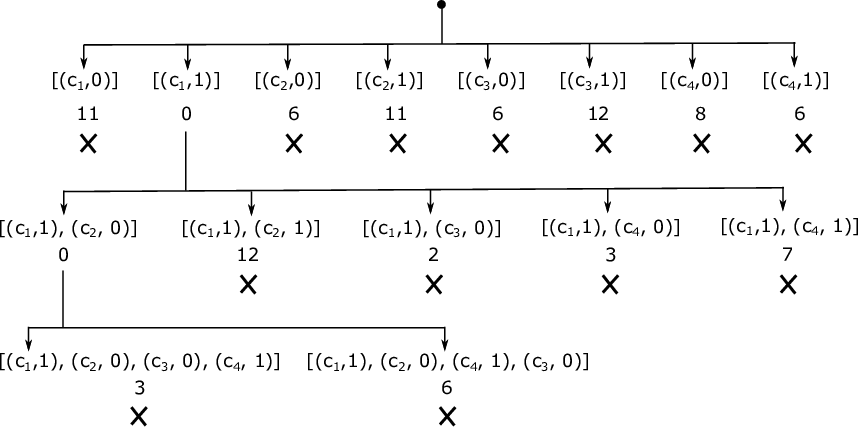
Consider the STV election of Table 1. The winner elimination upper bound is 2 votes and the Simple-STV bound is 6 votes. In Step 2, the current upper bound is initialised to 2. The partial candidate orders and are created, and assigned lower bounds by DistanceToSTV of 11, 0, 6, 11, 6, 12, 8, and 6, respectively. Only is added to in Step 9. Figure 4 visualises the search tree explored by margin-stv in this example.
Once the frontier is populated with partial orders of size one, Steps 10 to 14 expand these orders in the search for an alternate outcome for the election that requires the smallest degree of manipulation to realise. Partial orders with the smallest assigned lower bound are expanded in turn. A partial order is expanded by first removing it from the frontier (Step 12). For each candidate not mentioned in , two new partial orders are formed in which is elected () and eliminated () in successive iterations of the loop in Steps 18 to 26. If the new partial order is valid (i.e., it does not elect the same candidates elected in the original winners set ), it is evaluated with DistanceToSTV (Step 21). If contains all candidates (it is a complete order), it represents an alternate election outcome requiring vote manipulations to realise ( is computed by DistanceToSTV in Step 21). If is less than the current upper bound, , is replaced with (Step 23). If is not a complete order, it is added to if is less than (Step 26).
We repeatedly expand the partial order with the smallest assigned lower bound, updating the frontier , until is empty (there are no remaining partial orders that can be expanded). At this point, the algorithm terminates and returns the current upper bound as the election MOV in Step 15.
Example 3 (Example 2 cont).
The frontier, , now contains one partial order . The following partial orders are formed and evaluated with DistanceToSTV in successive executions of Step 19 and 21:
| Lower bound of 0 | |
| Lower bound of 12 | |
| Lower bound of 2 | |
| Invalid as the original winners and are both elected | |
| Lower bound of 3 | |
| Lower bound of 7 |
Only is added to in Step 26. At this point, , , and , is the next order expanded in Step 13. The following complete orders are formed in successive executions of Step 19 (in our implementation of margin-stv, we complete all partial orders formed in Step 19 with their ‘obvious’ ending if possible—i.e., if there is only one candidate remaining). All orders have a lower bound greater than the current upper bound of 2, and are pruned from consideration.
| DistanceToSTV evaluation of 3 | |
| Invalid as original winners and are elected | |
| Invalid as original winners and are elected | |
| DistanceToSTV evaluation of 6 |
After pruning all partial orders from , the frontier is empty and the algorithm returns the upper bound of 2 as the election MOV in Step 15. In this example, margin-stv has shown that there is no better manipulation (requiring fewer vote changes) than that inferred by the winner elimination upper bound.
In Steps 7 and 21, where DistanceToSTV is evaluated for a partial (or complete) order , we can use the lower bounding rule of Section 7.1 to compute an initial lower bound for , . If , the current upper bound, we need not solve DistanceToSTV as can immediately be pruned from consideration. If , we can solve DistanceToSTV to get a second lower bound for , . We can then assign to the maximum of the two lower bounds and . In Section 9, we examine the relative performance of margin-stv, in terms of the number of DistanceToSTV MINLPs solved and the runtime of the algorithm, in the setting where this extra lower bounding computation is performed, and when it is omitted.
8.1 Implementation Details
We use SCIP (Achterberg, 2009) to solve each MINLP formed by margin-stv. In practice, we have found that some instances of DistanceToSTV, even for small election instances, can be difficult for SCIP to solve in reasonable time. Consequently, we terminate MINLP solves if the time since a last improving solution has been found reaches a pre-specified time limit. If a partial order is being evaluated, and the MINLP is terminated before an optimal solution is found, the best objective value (a lower bound on the optimal objective) is assigned to as its lower bound. If a complete order is being evaluated, and the MINLP is terminated before finding an optimal solution, is inserted into the frontier with a lower bound equal to the best objective value of the MINLP, and the current upper bound is not revised (as would normally occur after evaluating a complete order). The result is that margin-stv may terminate with a frontier that contains a number of complete orders (that cannot be further expanded) with a smallest lower bound , and a current upper bound that is greater than (i.e., the algorithm returns with a lower and upper bound on the MOV, but not an exact value). This occurs for a number of elections in our test set in Section 9.
It is clear from the evaluation of margin-stv, in Section 9, on small STV elections (with candidate numbers ranging from 4 to 13) that it will not scale to more realistic elections with dozens of candidates. To improve its scalability, we vary the algorithm so that a MIP relaxation of the DistanceToSTV is constructed to evaluate each partial and complete order formed in Steps 6 and 19 of Figure 3. We consider two types of relaxation. The first replaces each bilinear term present in the MINLP (these terms appear in Constraints (17) and (20)) with McCormick (1976) inequalities. Each bilinear term , where and are continuous variables with domains and , is replaced with variable . Variable is defined by Equations (27) to (30). The optimal solution of the relaxed DistanceToSTV is a lower bound on that of the MINLP. The MOV computed by margin-stv, in this context, is a lower bound on the true MOV. An illustration of the McCormick envelope is shown in Figure 5(a) when is fixed.
| (27) | ||||
| (28) | ||||
| (29) | ||||
| (30) |
Our second relaxation replaces each bilinear term present in the MINLP (these terms appear in Constraints (17) and (20)) with a piecewise linear relaxation (specifically, a relaxation proposed by Gounaris et al. (2009)). The result is again a MIP relaxation of the DistanceToSTV whose optimal solution is a lower bound on that of the MINLP. Given a product of two continuous variables and (a bilinear term ), the piecewise linear relaxation we apply is defined as follows (replicated from the work of Gounaris et al. (2009)), where the variable replaces the bilinear term where it appears in the original MINLP. We divide the domain of into ranges ( ) and introduce a binary variable to indicate whether has a value in range . Constraint (31) ensures that only one can take on a value of 1. The domain of variable is . The variable defines the “deviation of variable from its lower bound , if ” and is set to 0 if the value of lies outside of this range (Gounaris et al., 2009). Figure 5(b) shows how the relaxation improves when we break the domain of into two ranges and .
| (31) | ||||||
| (32) | ||||||
| (33) | ||||||
| (34) | ||||||
| (35) | ||||||
| (36) | ||||||
| (37) | ||||||
| (38) | ||||||
In the DistanceToSTV MINLP, variables and (Constraint (17)), and and (Constraint (20)) participate in bilinear terms. We treat the transfer value of votes distributed from the candidate elected in round , , as in the piecewise linear relaxation scheme presented above, with variables (the total value of votes of signature in the tally of candidate at the start of round ) and (the number of transferable votes in the tally of the candidate elected in round ) as . In Section 9, we discretise the domain of into varying numbers of segments (by varying ), and compare the resulting lower bounds (on margins) found by margin-stv to the true MOV found when no such relaxation is used.
In their algorithm for computing margins in IRV elections, Magrino et al. (2011) recognise that their DistanceTo LP, defined to compute the smallest number of vote changes required to realise a particular (partial or complete) elimination order, need only consider a subset of possible vote signatures (in place of all possible partial and total orderings over the set of candidates). Given an elimination order , specifying which candidates are eliminated in each counting round, Magrino et al. (2011) note that classes of ballot signatures, denoted equivalence classes, will behave in the same way (be transferred between candidates in the same way) as counting progresses. Consequently, each DistanceTo LP need only contain variables defining the number of votes of each equivalence class present in the modified election profile. The definition of equivalence classes presented by Magrino et al. (2011) can be applied in the context of both IRV and STV elections, given an elimination sequence (for an IRV election) and a sequence of elections and eliminations (for an STV election). In our implementation of margin-stv, we define the DistanceToSTV MINLP (and its relaxations) over signature equivalence classes (i.e., the set contains the signatures of all equivalence classes, in place of all partial and total orders over the set of candidates ).
 |
 |
| (a) | (b) |
9 Evaluation
We first evaluate margin-stv on a set of small STV elections. To do so, we take 16 IRV elections conducted in the US between 2007 and 2010, and re-imagine them as STV elections with 2 available seats (Appendix A lists the names of each of these elections, alongside the number of candidates, and number of votes cast). The number of candidates in these elections range between 4 and 13. All experiments in this paper have been conducted on a machine with an Intel Xeon ES-2440 2.40GHz 6 core processor, and 64GB of RAM.
Table 4 reports the results of margin-stv – without and with the use of the lower bounding rule of Section 7.1 – on 16 small IRV (re-imagined as STV) elections. We record: the number of candidates in the election; the best computed upper bound on the MOV (the minimum of the winner elimination and Simple-STV upper bound); the MOV returned by margin-stv (or bounds on the MOV); the number of DistanceToSTV MINLPs solved by the algorithm; and the time taken by margin-stv to compute the MOV (in seconds). SCIP (Achterberg, 2009) is used to solve all DistanceToSTV MINLPs. We terminate each run of margin-stv after 12 hours, and infer a lower and upper bound on the MOV from the state of the frontier. Our algorithm did not terminate for three instances (13, 14, and 16) within 12 hours. In 11/16 instances, our algorithm could not produce an exact MOV, but a lower and upper bound on the MOV. In 7/11 instances, the lower and upper bound differed by only 1 vote (i.e., margin-stv was able to produce very tight bounds on the MOV). Table 4 shows that our lower bounding rule can, in some instances, reduce the runtime of the algorithm. For instances 1, 2, 10, and 12, runtimes are reduced by 107, 761, 106, and 1,635 seconds. Our lower bounding rule can increase the runtime of the algorithm—for instances 3 and 6, runtimes are increased by 185 and 378 seconds. Our lower bounding rule consistently reduces the number of MINLPs solved, but if these MINLPs are quickly deemed infeasible by SCIP (Achterberg, 2009), the additional time spent computing lower bounds for each partial order visited becomes an overhead.
| margin-stv | margin-stv with LB of Sec 7.1 | |||||||
| # | Best UB | MOV | MINLPs | Time | MOV | MINLPs | Time | |
| solved | (s) | solved | (s) | |||||
| 1 | 4 | 38,199 | 30,654 – 37,908 | 54 | 2,528 | 30,654 – 37,908 | 35 | 2,421 |
| 2 | 4 | 5,683 | 2,725 – 2,726 | 17 | 900 | 2,725 – 2,726 | 7 | 139 |
| 3 | 4 | 6,530 | 6,359 – 6,360 | 25 | 464 | 6,359 – 6,360 | 19 | 649 |
| 4 | 4 | 2,527 | 63 | 18 | 171 | 63 | 14 | 169 |
| 5 | 4 | 653 | 59 | 17 | 20 | 59 | 11 | 19 |
| 6 | 4 | 763 | 375 | 23 | 708 | 375 | 13 | 1,086 |
| 7 | 5 | 7,500 | 7,499 – 7,500 | 48 | 213 | 7,499 – 7,500 | 30 | 211 |
| 8 | 5 | 1,079 | 628 – 629 | 45 | 2,972 | 628 – 629 | 30 | 2,972 |
| 9 | 5 | 1,425 | 659 – 660 | 38 | 2,331 | 659 – 660 | 26 | 2,318 |
| 10 | 5 | 422 | 164 – 165 | 42 | 565 | 164 – 165 | 22 | 459 |
| 11 | 7 | 1,719 | 441 | 58 | 1 | 441 | 39 | 1 |
| 12 | 7 | 2,289 | 1,326– 1,327 | 2,247 | 13,693 | 1,326 – 1,327 | 1,006 | 12,058 |
| 13 | 8 | 2,857 | 1,216 – 1,576 | — | 1,309 – 1,576 | — | ||
| 14 | 11 | 1,178 | 309 – 1,178 | — | 351 – 1,178 | — | ||
| 15 | 11 | 63 | 4 | 244 | 107 | 4 | 190 | 106 |
| 16 | 13 | 2,188 | 823 – 2,188 | — | 0 – 2,188 | — | ||
| margin-stv | margin-stv with LB of Sec 7.1 | |||||||
| # | Exact MOV | MOV | MIPs | Time | MOV | MIPs | Time | |
| Bounds | (LB) | solved | (s) | (LB) | solved | (s) | ||
| 1 | 4 | 30,654 – 37,908 | 17,662 | 28 | 0.8 | 23,079 | 11 | 0.2 |
| 2 | 4 | 2,725 – 2,726 | 399 | 15 | 0.2 | 789 | 5 | 0.1 |
| 3 | 4 | 6,359 – 6,360 | 3245 | 28 | 0.4 | 6356 | 12 | 0.1 |
| 4 | 4 | 63 | 0 | 12 | 0.1 | 0 | 8 | 0.1 |
| 5 | 4 | 59 | 0 | 13 | 0.1 | 0 | 7 | 0.1 |
| 6 | 4 | 375 | 43 | 19 | 0.1 | 46 | 10 | 0.1 |
| 7 | 5 | 7,499 – 7,500 | 0 | 23 | 0.3 | 0 | 13 | 0.2 |
| 8 | 5 | 628 – 629 | 218 | 33 | 0.3 | 339 | 20 | 0.3 |
| 9 | 5 | 659 – 660 | 64 | 26 | 0.3 | 64 | 17 | 0.3 |
| 10 | 5 | 164 – 165 | 34 | 25 | 0.2 | 91 | 19 | 0.4 |
| 11 | 7 | 441 | 441 | 57 | 0.6 | 441 | 38 | 0.6 |
| 12 | 7 | 1,326 – 1,327 | 413 | 48 | 0.9 | 859 | 166 | 4 |
| 13 | 8 | 1,309 – 1,576 | 289 | 215 | 8 | 289 | 117 | 4 |
| 14 | 11 | 351 – 1,178 | 0 | 723 | 217 | 0 | 347 | 36 |
| 15 | 11 | 4 | 4 | 243 | 8 | 4 | 189 | 11 |
| 16 | 13 | 823 – 2,188 | 0 | — | 0 | 21,520 | 23,243 | |
Table 5 reports the results of the relaxed margin-stv algorithm (with bilinear terms replaced by McCormick (1976) inequalities) in each STV instance of Table 4, without and with the lower bounding rule of Section 7.1. CPLEX 12.5 is used to solve all DistanceToSTV MIPs formed by our margin-stv relaxations. We report the lower bound on the MOV found by margin-stv alongside the exact MOV (or bounds on the exact MOV) reported in Table 4. The lower bounds found by margin-stv (with McCormick (1976) inequalities) are often significantly lower than the exact MOV. Our lower bounding rule is beneficial in this setting – it often discovers tighter lower bounds on partial and complete orders than the MIP relaxation of DistanceToSTV (in 7/16 instances, applying the lower bounding rule results in a tighter lower bound being found by relaxed margin-stv), and reduces runtimes significantly for larger instances.
| # | Exact MOV | MOV | MIPs | Time | MOV | MIPs | Time |
|---|---|---|---|---|---|---|---|
| Bounds | LB | solved | (s) | LB | solved | (s) | |
| 1 | 30,654 – 37,908 | 28,038 | 12 | 1 | 29,020 | 12 | 1 |
| 2 | 2,725 – 2,726 | 2,265 | 6 | 0.5 | 2,512 | 6 | 1 |
| 3 | 6,359 – 6,360 | 6,356 | 13 | 0.4 | 6,356 | 17 | 2 |
| 4 | 63 | 0 | 8 | 0.1 | 0 | 8 | 0.1 |
| 5 | 59 | 0 | 7 | 0.4 | 10 | 9 | 1 |
| 6 | 375 | 327 | 10 | 0.2 | 337 | 10 | 0.6 |
| 7 | 7,499 – 7,500 | 5,168 | 14 | 0.9 | 6,347 | 28 | 4 |
| 8 | 628 – 629 | 531 | 24 | 2 | 581 | 25 | 7 |
| 9 | 659 – 660 | 558 | 19 | 0.9 | 609 | 19 | 3 |
| 10 | 164 – 165 | 133 | 19 | 4 | 141 | 19 | 3 |
| 11 | 441 | 441 | 38 | 0.7 | 441 | 38 | 0.8 |
| 12 | 1,326 – 1,327 | 1049 | 486 | 37 | 1,211 | 698 | 83 |
| 13 | 1,309 – 1,576 | 1321 | 538 | 65 | 1,431 | 636 | 243 |
| 14 | 351 – 1,178 | 53 | 84 | 22 | 602 | 3,008 | 2,900 |
| 15 | 4 | 4 | 189 | 22 | 4 | 189 | 27 |
| 16 | 823 – 2,188 | 760 | 7,025 | 35,583 | 95 | — | |
| # | Exact MOV | MOV | MIPs | Time | MOV | MIPs | Time |
| Bounds | LB | solved | (s) | LB | solved | (s) | |
| 1 | 20,654 – 37,908 | 29,549 | 12 | 3 | 29,968 | 12 | 3 |
| 2 | 2,725 – 2,726 | 2,582 | 6 | 2 | 2,609 | 6 | 1 |
| 3 | 6,359 – 6,360 | 6,356 | 17 | 2 | 6,356 | 17 | 1 |
| 4 | 63 | 0 | 11 | 0.4 | 0 | 11 | 1 |
| 5 | 59 | 28 | 9 | 1 | 35 | 9 | 1 |
| 6 | 375 | 351 | 10 | 1 | 358 | 10 | 2 |
| 7 | 7,499 – 7,500 | 6,721 | 29 | 3 | 6,923 | 29 | 4 |
| 8 | 628 – 629 | 598 | 25 | 10 | 606 | 25 | 12 |
| 9 | 659 – 660 | 623 | 19 | 5 | 638 | 20 | 4 |
| 10 | 164 – 165 | 147 | 19 | 6 | 155 | 19 | 6 |
| 11 | 441 | 441 | 38 | 0.6 | 441 | 38 | 1 |
| 12 | 1,326 – 1,327 | 1,221 | 700 | 105 | 1,257 | 758 | 185 |
| 13 | 1,309 – 1,576 | 1,468 | 747 | 452 | 1,486 | 754 | 638 |
| 14 | 351 – 1,178 | 785 | 10,511 | 15,732 | 878 | 13,786 | 28,909 |
| 15 | 4 | 4 | 189 | 33 | 4 | 189 | 39 |
| 16 | 823 – 2,188 | 17 | — | 0 | — | ||
Relaxed margin-stv (with McCormick (1976) inequalities and our lower bounding rule) can compute a lower bound on the margin in each of our 16 STV instances within 12 hours. However, in 5/16 instances a trivial lower bound of 0 is found. We consider whether solving a piecewise linear relaxation of each DistanceToSTV MINLP, as described in Section 8.1, results in margin-stv finding better lower bounds. Table 6 reports the results of piecewise-relaxed margin-stv (with the use of our lower bounding rule) given varying (with higher values of forming a more accurate relaxation of each DistanceToSTV MINLP). In general, the resulting MOV lower bounds increase as increases. The counter-example is instance 16, for which margin-stv computes lower bounds of 760, 95, 17, and 0 for 5, 10, 15, and 20. As increases, the MIP relaxations solved throughout the algorithm become more complex and time consuming to solve. Consequently, margin-stv makes less progress through the space of partial orders in instance 16 within the 12 hour time limit. In the setting, margin-stv finds reasonable lower bounds in most instances. The exact MOV is found in 2 instances (11 and 15). In instance 13, we find a margin that lies within the bounds found on the MOV by the exact algorithm. Across instances 1 to 3, 6, 8 to 10, 12, and 16, the MOV lower bounds discovered are, on average, 14.4% below the exact MOV (or lower bound on the MOV found by the exact algorithm). In instances 4 and 5, piecewise-relaxed margin-stv finds trivial lower bounds of 0, however the exact MOV in these instances is small (63 and 59 votes, respectively).
9.1 Real-World STV Elections
In the preceding section we have evaluated margin-stv on a series of IRV elections (re-imagined as STV elections with 2 seats) held in the US between 2007 and 2010. The number of candidates in these elections range from 4 to 13. STV elections often involve a large number of candidates. In the 2012 election of senators to the ACT senate in Australia, 5-7 senators were elected in each of 3 districts. An STV election was held for each district, involving 20, 26, and 28 candidates. In the 2014 Victorian senate election in Australia, 5 senators were elected in each of 5 districts. The number of candidates in these elections ranged from 37 to 52. The use of margin-stv for elections of this size, without relaxation, is not feasible (due to the complexity of the DistanceToSTV MINLPs that must be solved). We demonstrate the value of our margin-stv algorithm for computing lower bounds on the margin in a number of real-world STV elections.
In addition to the use of MINLP relaxations (McCormick (1976) inequalities and piecewise-linear relaxations), we parallelise the exploration of the frontier of partial candidate orders. In place of selecting one partial candidate order to expand (at Step 13 of Figure 3), we select the first (where is a parameter) orders in the frontier . Each of these orders is expanded in parallel, and the frontier updated accordingly – the children of all expanded orders with DistanceToSTV evaluations that are less than the current upper bound are inserted into the frontier. This upper bound is revised, and orders pruned from the frontier, when a complete order is found with a DistanceToSTV evaluation that is lower than the current upper bound.
The number of variables and constraints in the DistanceToSTV models solved by margin-stv is determined by the number of candidates in the orders being evaluated. In most STV elections, the number of available seats is much less than the number of candidates. Consequently, these orders will contain lengthy sequences of candidate eliminations. To limit the memory and solve time requirements of the DistanceToSTV models formed by margin-stv, we group these sequences of eliminated candidates together, ignoring constraints that enforce their relative elimination order (i.e., these candidates are effectively eliminated in a single round of counting). Grouping eliminated candidates together reduces the number of constraints required, and significantly reduces the number of vote equivalence classes that need to be considered, in each DistanceToSTV model. This grouping adds an additional level of relaxation to the algorithm.
We consider, in this section, the performance of margin-stv on 28 STV elections. We consider: the 2013 and 2016 election of 2 candidates to the Federal Senate for the Australian Capital Territory (ACT) and Northern Territory (NT); the 2002 election of 4, 3, and 5 candidates to the lower house of the Irish parliament (the Dáil Éireann) representing the Dublin North, Dublin West, and Meath constituencies; and 21 STV elections electing 3 to 4 candidates (out of 8 to 13, per ward) to the Glasgow City Council in 2007. Data for the Irish and Scottish STV elections were obtained from PrefLib22 2 www.preflib.org. In each experiment reported in this section, margin-stv has been afforded a time limit of 24 hours. If this time limit is reached, and the algorithm has not converged, we report the best lower bounds on the MOV computed in that time period. Unless otherwise stated, we set and run margin-stv with increasing values of (from to ) until the resulting lower bound does not improve, or is within 10% of the best known upper bound.
9.2 2002 Irish General Election
We first consider the 2002 election of 4, 3, and 5 candidates (out of 13, 9, and 15) to the Irish lower house to represent Dublin North, Dublin West, and Meath. Table 7 reports, for each election, the quota, number of votes cast, and the best known upper bound on the MOV (computed as per Figure 2 and Section 5). For increasing values of , we report the lower bound on the MOV computed by margin-stv over a 24 hour period, the runtime (in seconds) of the algorithm (if less than 24 hours), and the number of MIPs solved.
| Election | Seats | Quota | Votes | Upper | Lower | Time (s) | MIPs | ||
| cast | Bound | Bound | Solved | ||||||
| on MOV | on MOV | ||||||||
| Dublin North | 4 | 13 | 8,789 | 43,942 | 211 | 5 | 0 | 46 | 400 |
| 15 | 181 | 2,905 | 487 | ||||||
| 25 | 185 | 10,808 | 276 | ||||||
| 35 | 199 | 50,994 | 394 | ||||||
| Dublin West | 3 | 9 | 7,498 | 29,988 | 385 | 5 | 0 | 15 | 143 |
| 15 | 153 | 241 | 147 | ||||||
| 25 | 211 | 506 | 153 | ||||||
| 35 | 235 | 1,628 | 151 | ||||||
| 60 | 257 | 3,914 | 155 | ||||||
| 80 | 267 | 14,649 | 161 | ||||||
| 100 | 269 | 38,660 | 157 | ||||||
| Meath | 5 | 15 | 10,681 | 64,081 | 1,135 | 5 | 275 | – | 1,997 |
| 15 | 275 | 72,349 | 549 |
| Election | Seats | Quota | Votes | MOV | MOV | Time | MIPs | ||
| cast | Upper | Lower | (s) | Solved | |||||
| Bound | Bound | ||||||||
| Linn | 4 | 11 | 1,914 | 9,567 | 221 | 5 | 94 | 1,147 | 1,840 |
| 15 | 139 | – | 5,867 | ||||||
| Newlands | 3 | 9 | 2,164 | 8,654 | 88 | 5 | 47 | 14 | 203 |
| 15 | 76 | 78 | 284 | ||||||
| 25 | 81 | 363 | 284 | ||||||
| Greater Pollock | 4 | 9 | 1,737 | 8,682 | 223 | 5 | 125 | 1,866 | 1,647 |
| 15 | 197 | 38,428 | 3,349 | ||||||
| 25 | 159* | – | 2,304 | ||||||
| Craigton | 4 | 10 | 2,211 | 11,052 | 93 | 5 | 0 | 62 | 174 |
| 15 | 0 | 493 | 175 | ||||||
| 25 | 25 | 1,176 | 168 | ||||||
| 35 | 37 | 11,321 | 179 | ||||||
| 50 | 43 | 39,892 | 188 | ||||||
| 80 | 31* | – | 164 | ||||||
| Govan | 4 | 11 | 1,913 | 9,560 | 278 | 5 | 149 | – | 10,808 |
| 15 | 131* | – | 5,226 | ||||||
| Pollockshields | 3 | 9 | 2,392 | 9,567 | 30 | 5 | 0 | 1 | 39 |
| 15 | 0 | 6 | 39 | ||||||
| 25 | 2 | 19 | 39 | ||||||
| 35 | 4 | 20 | 39 | ||||||
| 80 | 4 | 347 | 39 | ||||||
| 100 | 6 | 681 | 39 | ||||||
| Langside | 3 | 8 | 2,334 | 9,334 | 246 | 5 | 124 | 25 | 224 |
| 15 | 193 | 555 | 545 | ||||||
| 25 | 209 | 3,350 | 553 | ||||||
| 35 | 217 | 7,266 | 742 | ||||||
| 45 | 221 | 14,495 | 746 | ||||||
| 55 | 224 | 19,341 | 752 | ||||||
| Southside Central | 4 | 9 | 1,748 | 8,738 | 231 | 5 | 113 | 1,306 | 1,418 |
| 15 | 187 | 68,537 | 2,313 | ||||||
| 25 | 118* | – | 1,120 | ||||||
| Calton | 3 | 10 | 1,300 | 5,199 | 959 | 5 | 215 | 18,369 | 39,356 |
| 15 | 130* | – | 20,048 | ||||||
| Anderston | 4 | 9 | 1,381 | 6,900 | 106 | 5 | 3 | 57 | 168 |
| 15 | 64 | 5,596 | 346 | ||||||
| 25 | 85 | 16,784 | 407 | ||||||
| 35 | 94 | 51,571 | 517 | ||||||
| Hillhead | 4 | 10 | 1,797 | 8,984 | 112 | 5 | 0 | 35 | 271 |
| 15 | 41 | 1,621 | 270 | ||||||
| 25 | 55 | 8,277 | 270 | ||||||
| 35 | 58 | 27,949 | 265 | ||||||
| 45 | 0* | – | 251 |
| Election | Seats | Quota | Votes | MOV | MOV | Time | MIPs | ||
| cast | Upper | Lower | (s) | Solved | |||||
| Bound | Bound | ||||||||
| Partick West | 4 | 9 | 2,549 | 12,744 | 194 | 5 | 18 | 22 | 166 |
| 15 | 133 | 728 | 207 | ||||||
| 25 | 174 | 6,407 | 311 | ||||||
| 35 | 187 | 10,343 | 354 | ||||||
| Garscadden | 4 | 10 | 2,033 | 10,160 | 449 | 5 | 197 | – | 5,080 |
| 15 | 96* | – | 780 | ||||||
| Drumchapel | 4 | 10 | 1,737 | 8,680 | 1,325 | 5 | 335 | 19,325 | 16,257 |
| 15 | 0* | – | 353 | ||||||
| Maryhill | 4 | 8 | 1,981 | 9,901 | 292 | 5 | 70 | 140 | 329 |
| 15 | 203 | 11,580 | 606 | ||||||
| 25 | 226 | 25,849 | 776 | ||||||
| 35 | 234 | 78,380 | 747 | ||||||
| 45 | 194* | – | 482 | ||||||
| Canal | 4 | 11 | 1,725 | 8,624 | 148 | 5 | 68 | 487 | 576 |
| 15 | 98 | 9,384 | 729 | ||||||
| 25 | 108 | 36,690 | 852 | ||||||
| 35 | 109 | 79,946 | 844 | ||||||
| 45 | 69* | – | 300 | ||||||
| Springburn | 3 | 10 | 1,353 | 5,410 | 1,014 | 5 | 447 | 22,772 | 37,236 |
| 15 | 305* | – | 3,979 | ||||||
| East Centre | 4 | 13 | 1,816 | 9,078 | 134 | 5 | 73 | 26,753 | 16,360 |
| 15 | 71* | – | 10,389 | ||||||
| Shettleston | 4 | 11 | 1,761 | 8,803 | 355 | 5 | 158 | – | 13,014 |
| 15 | 145* | – | 4,817 | ||||||
| Baillieston | 4 | 11 | 2,076 | 10,376 | 108 | 5 | 0 | 457 | 266 |
| 15 | 38 | 2,088 | 347 | ||||||
| 25 | 46 | 11,122 | 345 | ||||||
| 35 | 58 | 49,942 | 383 | ||||||
| 45 | 64 | 74,870 | 390 | ||||||
| 55 | 8* | – | 300 | ||||||
| North East | 4 | 10 | 1,673 | 8,363 | 911 | 5 | 275 | 52,653 | 9,967 |
| 15 | 60* | – | 385 |
9.3 2007 Glasgow City Council
In the 2007 Glasgow City Council election, 3 to 4 candidates (out of 8 to 13) were elected in 21 STV elections (one for each of 21 wards). Tables 8 and 9 report the quota, number of votes cast, and the best known upper bound on the MOV (computed as per Figure 2 and Section 5). For increasing values of , we report the lower bound on the MOV computed by margin-stv over a 24 hour period, the runtime (in seconds) of the algorithm (if less than 24 hours), and the number of MIPs solved. Instances where the MOV lower bound computed within 24 hours reduces as is increased are marked with an asterisk. Increasing increases the complexity, and solve times, of the MIPs being solved. These instances demonstrate that, as increases, the branch-and-bound search conducted by margin-stv may make less progress over the 24 hour period, resulting in a lower (rather than improved) lower bound on the MOV.
9.4 2013 and 2016 NT and ACT Federal Senate
Table 10 reports lower bounds on the MOV computed for the 2013 and 2016 ACT and NT Federal Senate elections. While these elections have a small number of seats (2), there are many candidates (between 19 and 27). In each of these elections, the two winning candidates have orders of magnitude more votes in their initial tallies than all others. We expect the margin in these elections to be reasonably high (certainly greater than a few hundred votes) as we need to change enough votes to ensure one of these candidates is not awarded a seat (and that one alternate candidate is awarded a seat). The MOV lower bounds found by margin-stv in Table 10 are likely to be much lower than the true margins.
| Election | Seats | Quota | Votes | Upper | Lower | Time (s) | MIPs | ||
|---|---|---|---|---|---|---|---|---|---|
| cast | Bound | Bound | Solved | ||||||
| on MOV | on MOV | ||||||||
| 2013 NT | 2 | 24 | 34,494 | 103,479 | 25,777 | 5 | 223 | – | 561,999 |
| 2016 NT | 2 | 19 | 34,010 | 102,027 | 23,373 | 5 | 3121 | – | 219,876 |
| 2013 ACT | 2 | 27 | 82,248 | 246,742 | 35,476 | 5 | 82 | – | 112,629 |
| 2016 ACT | 2 | 22 | 84,923 | 254,767 | 44,499 | 5 | 205 | – | 86,825 |
The elections of Table 10 follow a similar pattern – a candidate is awarded a seat in the first round of counting, and then a long sequence of candidates are eliminated before a second candidate achieves a quota and is awarded a seat. In these circumstances, we can compute a lower bound on the MOV under the assumption that we cannot change who is elected and eliminated in the first rounds of counting. For large values of , this assumption prunes significant portions of the space of possible elimination and election sequences from consideration. Consider the 2013 ACT election, in which the two available seats are awarded in rounds 1 and 24. If we assumed the first 20 rounds () are fixed (i.e., the first winner is elected in round 1, and the candidates eliminated in rounds 2 to 20 are still eliminated, at some point, between rounds 2 to 20), Table 11 reports our computed lower bounds on the MOV for this election.
| Lower Bound | Time (s) | MIPs | |
|---|---|---|---|
| on MOV | Solved | ||
| 5 | 5879 | 117 | 41 |
| 25 | 5879 | 4899 | 111 |
| 50 | 5911 | 12,386 | 112 |
| 80 | 5919 | 18,604 | 112 |
The lower bounds reported in Table 11, for the 2013 ACT Federal Senate election, are not guaranteed lower bounds on the true margin of victory of the election. If we take the minimal manipulation discovered by margin-stv in the case, and simulate the modified election with the suggested vote changes put in place, we find that the original winning candidates ( and ) are given a seat (in rounds 1 and in the last round). However, the tallies of and the runner up , at the point at which is eliminated differ in only 159 votes. We consider an additional manipulation that awards 80 additional first preference votes to the runner up , and removes 80 first preference votes from (we effectively swap 80 votes that ranked first with a ranking that has in first place). Simulating this modified election gives us a different outcome, with candidates and elected to a seat (in rounds 1 and in the last round). For this election, we now know that the MOV is no more than 5,999 votes – we were able to find an alternate outcome by modifying 5,999 votes to an alternate ranking. The upper bounds found by the winner elimination upper bound method of Figure 2, and the simple upper bound method of Section 5, are much higher than the true MOV. This analysis suggests there are alternate ways of using margin-stv for computing lower and upper bounds on the MOV for large, and challenging, elections (with many seats or large numbers of candidates). In future work, we aim to explore this further.
10 Concluding Remarks
In this paper we develop an algorithm, margin-stv, for computing exact margins of victory in STV elections, assuming the use of the Inclusive Gregory method of surplus distribution. The algorithm is based on solving a mixed-integer nonlinear formulation for the problem of computing a minimal manipulation to achieve a desired election order. We are able to compute exact margins of victory for small elections, e.g. less than 12 candidates and 2 seats. For larger, real elections margin-stv is able to compute reasonable lower bounds within 24 hours (as demonstrated on 28 real-world STV elections). The algorithm struggles on elections with large numbers of candidates, essentially since the search space grows as the factorial of the number of candidates, but provides an important first step in tackling this important and challenging problem.
As future work we plan to adapt the margin-stv algorithm to answer specific questions such as the influence of instances of multiple-voting on election outcomes, and the impact of losing votes, similar to our prior work (Blom et al., 2016) on Instant Runoff Voting (IRV) elections. In addition, we aim to explore how applying the algorithm to the tail of an STV election (i.e., by fixing the elections and eliminations that occur in the first rounds of counting) can be used within a practical algorithm for computing improved lower and upper bounds on the MOV in challenging instances (with a large number of seats or candidates).
Appendix A US Election Data (2007 to 2010)
In the experiments of Section 9 we reimagine a series of 16 IRV elections conducted in the US between 2007 and 2010 as STV elections with 2 available seats. Table 12 records the name, number of candidates, and number of votes cast, for each of these 16 elections. Candidate numbers range between 4 and 13.
| # | Election Name | Candidates | Votes Cast |
| 1 | Pierce 2008 County Auditor | 4 | 159,987 |
| 2 | Pierce 2008 City Council | 4 | 43,661 |
| 3 | San Leandro 2010 Mayor | 4 | 23,494 |
| 4 | Oakland 2010 D6 City Council | 4 | 14,040 |
| 5 | Berkeley 2010 D8 City Council | 4 | 5,333 |
| 6 | Berkeley 2010 D7 City Council | 4 | 4,862 |
| 7 | Pierce 2008 County Executive | 5 | 312,771 |
| 8 | Berkeley 2010 D4 City Council | 5 | 5,708 |
| 9 | Berkeley 2010 D1 City Council | 5 | 6,426 |
| 10 | Aspen 2009 Mayor | 5 | 2,544 |
| 11 | Pierce 2008 County Assessor | 7 | 43,661 |
| 12 | San Leandro 2010 D5 City Council | 7 | 23,494 |
| 13 | Oakland 2010 D4 City Council | 8 | 23,884 |
| 14 | Oakland 2010 Mayor | 11 | 122,268 |
| 15 | Aspen 2009 City Council | 11 | 2,544 |
| 16 | San Francisco 2007 Mayor | 13 | 149,465 |
References
- Achterberg [2009] T. Achterberg. SCIP: Solving constraint integer programs. Mathematical Programming Computation, 1(1):1–41, 2009. http://mpc.zib.de/index.php/MPC/article/view/4.
- Bartholdi III and Orlin [1991] J. J. Bartholdi III and J. B. Orlin. Single transferable vote resists strategic voting. Social Choice and Welfare, 8(4):341–354, 1991.
- Blom et al. [2016] M. Blom, P. J. Stuckey, V. Teague, and R. Tidhar. Efficient Computation of Exact IRV Margins. In European Conference on AI (ECAI), pages 480–487, 2016.
- Brandt et al. [2016] F. Brandt, V. Conitzer, U. Endriss, A. D. Procaccia, and J. Lang. Handbook of computational social choice. Cambridge University Press, 2016.
- Cary [2011] D. Cary. Estimating the margin of victory for instant-runoff voting. In USENIX Accurate Electronic Voting Technology Workshop: Workshop on Trustworthy Elections, USENIX Association Berkeley, CA, USA, 2011.
- Chilingirian et al. [2016] B. Chilingirian, Z. Perumal, R. L. Rivest, G. Bowland, A. Conway, P. B. Stark, M. Blom, C. Culnane, and V. Teague. Auditing australian senate ballots. Technical report, arXiv.org, 2016. URL https://arxiv.org/abs/1610.00127.
- Conitzer et al. [2003] V. Conitzer, J. Lang, and T. Sandholm. How many candidates are needed to make elections hard to manipulate? In Proceedings of the 9th Conference on Theoretical Aspects of Rationality and Knowledge, pages 201–214, Bloomington, Indiana, USA, 2003. ACM.
- Conitzer et al. [2007] V. Conitzer, T. Sandholm, and J. Lang. When are elections with few candidates hard to manipulate? Journal of the ACM (JACM), 54(3):14, 2007.
- Faliszewski et al. [2009] P. Faliszewski, E. Hemaspaandra, and L. Hemaspaandra. How Hard Is Bribery in Elections? Journal of Artificial Intelligence Research, 35:485–532, 2009.
- Farrell and McAllister [2005] D. Farrell and I. McAllister. Australia: The Alternative Vote in a Compliant Political Culture. In M. Gallagher and P. Mitchell, editors, The Politics of Electoral Systems, pages 79–97. Oxford University Press, Oxford, 2005.
- Gounaris et al. [2009] C. E. Gounaris, R. Misener, and C. A. Floudas. Computational Comparison of Piecewise-Linear Relaxations for Pooling Problems. Industrial and Engineering Chemistry Research, 48:5742–5766, 2009.
- Kaczmarczyk and Faliszewski [2016] A. Kaczmarczyk and P. Faliszewski. Algorithms for Destructive Shift Bribery. In Proceedings of the 2016 International Conference on Autonomous Agents & Multiagent Systems (AAMAS), pages 305–313, 2016.
- Magrino et al. [2011] T. Magrino, R. Rivest, E. Shen, and D. Wagner. Computing the margin of victory in IRV elections. In USENIX Accurate Electronic Voting Technology Workshop: Workshop on Trustworthy Elections, USENIX Association Berkeley, CA, USA, 2011.
- McCormick [1976] G. P. McCormick. Computability of Global Solutions to Factorable Nonconvex Programs: Part I – Convex Underestimating Problems. Mathematical Programming, 10:147–175, 1976.
- Miragliotta [2004] N. L. Miragliotta. Little differences, big effects: An example of the importance of choice of method for transferring surplus votes in PR-STV voting systems. Representation, 41:15–24, 2004.
- Narodytska and Walsh [2014] N. Narodytska and T. Walsh. The computational impact of partial votes on strategic voting. In Proceedings of the European Conference on Artificial Intelligence (ECAI), pages 657–662, 2014.
- Rothe and Schend [2013] J. Rothe and L. Schend. Challenges to complexity shields that are supposed to protect elections against manipulation and control: a survey. Annals of Mathematics and Artificial Intelligence, 68(1-3):161–193, 2013. ISSN 1012-2443.
- Sarwate et al. [2013] A. Sarwate, S. Checkoway, and H. Shacham. Risk-limiting audits and the margin of victory in nonplurality elections. Statistics, Politics, and Policy, 4(1):29–64, Jan. 2013.
- Schürmann [2017] C. Schürmann. Automatic margin computation for risk-limiting audits. In Electronic Voting: First International Joint Conference, E-Vote-ID 2016, pages 18–37, Bregenz, Austria, 2017. Springer.
- Weeks [2011] L. Weeks. Tolerable Chance or Undesirable Arbitrariness? Distributing Surplus Votes Under PR-STV. Parliamentary Affairs, 64:530–551, 2011.
- Xia [2012] L. Xia. Computing the margin of victory for various voting rules. In Proceedings of the ACM Conference on Electronic Commerce (EC), pages 982–999, 2012.