跳到论文正文
W Papers独立论文阅读器 arXiv:1703.03182 论文正文 计算阅读时间 · 0%
引用这篇论文根据当前论文元数据生成,正式投稿前建议核对。


License: arXiv.org perpetual non-exclusive license
arXiv:1703.03182v2 [math.NT] 10 Oct 2017

On the rank and the convergence rate towards the Sato–Tate measureThanks: Fité was funded by the German Research Council via SFB/TR 45 and by the Excellence Program María de Maeztu MDM-2014-0445. Guitart was partially supported by MTM2015-66716-P. Both authors were partially supported by MTM2015-63829-P. This project has received funding from the European Research Council (ERC) under the European Union’s Horizon 2020 research and innovation programme (grant agreement No 682152).

Francesc Fité Address: Departament de Matemàtiques, Universitat Politècnica de Catalunya/BGSmath
Edifici Omega, C/Jordi Girona 1–3
08034 Barcelona, Catalonia
Email address: francesc.fite@gmail.com URL: https://mat-web.upc.edu/people/francesc.fite/
and Xavier Guitart Address: Departament de Matemàtiques i Informàtica
Universitat de Barcelona
Gran via de les Corts Catalanes, 585
08007 Barcelona, Catalonia
Email address: xevi.guitart@gmail.com
Date: August 24, 2026
Abstract.

Let AA be an abelian variety defined over a number field and let GG denote its Sato–Tate group. Under the assumption of certain standard conjectures on LL-functions attached to the irreducible representations of GG, we study the convergence rate of any virtual character of GG. We find that this convergence rate is dictated by several arithmetic invariants of AA, such as its rank or its Sato–Tate group GG. The results are consonant with some previous experimental observations, and we also provide additional numerical evidence consistent with them. The techniques that we use were introduced by Sarnak in a letter to Mazur, in order to explain the bias in the sign of the Frobenius traces of an elliptic curve without complex multiplication defined over ℚ\mathbb{Q}. We show that the same methods can be adapted to study the convergence rate of the characters of its Sato–Tate group, and that they can also be employed in the more general case of abelian varieties over number fields. A key tool in our analysis is the existence of limiting distributions for automorphic LL-functions, which is due to Akbary, Ng, and Shahabi.

2010 Mathematics Subject Classification
11G05, 11G10, 14G10, 11M50

1. Introduction

Let kk be a number field and AA be an abelian variety defined over kk of dimension g≥1g\geq 1. Following Serre [Ser94], Banaszak and Kedlaya [BK16a] have attached to AA a compact real Lie subgroup GG of USp⁡(2​g)\mathrm{USp}(2g), the so-called Sato–Tate group of AA, with the conjectural property that it governs the distribution of the Frobenius elements attached to AA. 11 1 The construction of [BK16a] is in fact more general and it applies to odd weight motives.

In order to make a more precise statement, let us introduce some notations. Let ℓ\ell be a rational prime and let Vℓ​(A)V_{\ell}(A) denote the (rational) ℓ\ell-adic Tate module of AA. The action of the absolute Galois group GkG_{k} of kk on Vℓ​(A)V_{\ell}(A) gives rise to an ℓ\ell-adic representation

(1.1) ϱA:Gk→Aut⁡(Vℓ​(A)).\varrho_{A}:G_{k}\rightarrow\operatorname{Aut}(V_{\ell}(A))\,.

Denote by PP the set of nonzero prime ideals of kk lot lying over ℓ\ell and of good reduction for AA, that is, the set of nonzero prime ideals of kk not dividing the conductor 𝔑\mathfrak{N} of AA. For a prime 𝔭{\mathfrak{p}} in PP, set

(1.2) L𝔭​(A,T):=det(1−ϱA​(Frob𝔭)​T|Vℓ​(A)),L_{\mathfrak{p}}(A,T):=\det(1-\varrho_{A}(\operatorname{Frob}_{\mathfrak{p}})T\,|\,V_{\ell}(A))\,,

where Frob𝔭\operatorname{Frob}_{\mathfrak{p}} denotes a Frobenius element at 𝔭{\mathfrak{p}}. Attached to 𝔭{\mathfrak{p}}, one can construct a semisimple conjugacy class y𝔭y_{\mathfrak{p}} in the set of conjugacy classes YY of GG such that

(1.3) det(1−y𝔭​T)=L𝔭​(A,T/|𝔭|),\det(1-y_{{\mathfrak{p}}}T)=L_{\mathfrak{p}}(A,T/\sqrt{|{\mathfrak{p}}|})\,,

where |𝔭||{\mathfrak{p}}| denotes the absolute norm of 𝔭{\mathfrak{p}}. We will refer to the projection μ\mu of the Haar measure μG\mu_{G} of GG on YY as the Sato–Tate measure of AA. The conjectural property of GG that we have alluded to before predicts that the sequence {y𝔭}𝔭∈P\{y_{{\mathfrak{p}}}\}_{{\mathfrak{p}}\in P}, where the ideals in PP are ordered according to their absolute norm, is equidistributed on YY with respect to μ\mu.

Let us recall what this means. For x>0x>0, let π⁡(x)\pi(x) denote the number of primes 𝔭{\mathfrak{p}} in PP such that |𝔭|≤x|{\mathfrak{p}}|\leq x. Set

μx:=1π⁡(x)​∑|𝔭|≤xδy𝔭,\mu_{x}:=\frac{1}{\pi(x)}\sum_{|{\mathfrak{p}}|\leq x}\delta_{y_{{\mathfrak{p}}}}\,,

where δy𝔭\delta_{y_{\mathfrak{p}}} denotes the Dirac measure at y𝔭y_{\mathfrak{p}} and the sum runs over primes of PP such that |𝔭|≤x|{\mathfrak{p}}|\leq x. From now on, we make the convention that all sums of terms involving y𝔭y_{\mathfrak{p}} run over primes 𝔭∈P{\mathfrak{p}}\in P. By definition, we say that {y𝔭}𝔭∈P\{y_{{\mathfrak{p}}}\}_{{\mathfrak{p}}\in P} is equidistributed on YY with respect to μ\mu, or simply μ\mu-equidistributed on YY, if

(1.4) μx→μ weakly as x→∞.\mu_{x}\rightarrow\mu\qquad\text{ weakly as }\qquad x\rightarrow\infty\,.

As explained in [Ser68, Prop. 2, App. Chap. I], the sequence {y𝔭}𝔭∈P\{y_{\mathfrak{p}}\}_{{\mathfrak{p}}\in P} is μ\mu-equidistributed on YY if and only if for every irreducible character χ\chi of GG one has that

(1.5) limx→∞1π⁡(x)​∑|𝔭|≤xχ⁡(y𝔭)=δ⁡(χ),\lim_{x\rightarrow\infty}\frac{1}{\pi(x)}\sum_{|{\mathfrak{p}}|\leq x}\chi(y_{\mathfrak{p}})=\delta(\chi)\,,

where δ⁡(χ)\delta(\chi) is 11 or 00 depending on whether χ\chi is trivial or not.22 2 More generally and for future use, given a virtual character φ\varphi of GG, let δ⁡(φ)\delta(\varphi) denote the multiplicity of the trivial representation in φ\varphi. Recall that, by the Prime Number Theorem, (1.5) is equivalent to

(1.6) limx→∞log⁡(x)x​∑|𝔭|≤xχ⁡(y𝔭)=δ⁡(χ),\lim_{x\rightarrow\infty}\frac{\log(x)}{x}\sum_{|{\mathfrak{p}}|\leq x}\chi(y_{\mathfrak{p}})=\delta(\chi)\,,

and that, by the Abel summation trick, (1.5) is also equivalent to

(1.7) ∑|𝔭|≤xχ⁡(y𝔭)​log⁡(|𝔭|)=δ⁡(χ)​x+o⁡(x).\sum_{|{\mathfrak{p}}|\leq x}\chi(y_{\mathfrak{p}})\log(|{\mathfrak{p}}|)=\delta(\chi)x+o(x)\,.

It is of crucial importance that (1.5) is connected, via the Wiener–Ikehara Theorem, to the theory of LL-functions (see [Ser68, Thm. 1, App. Chap. I]). For 𝔭∈P\mathfrak{p}\in P, define the polynomial

L𝔭​(χ,T):=det(1−ϱ⁡(y𝔭)​T),L_{\mathfrak{p}}(\chi,T):=\det(1-\varrho(y_{{\mathfrak{p}}})T)\,,

where ϱ\varrho is an irreducible representation of GG of character χ\chi. The degree dχ​(𝔭)d_{\chi}({\mathfrak{p}}) of L𝔭​(χ,T)L_{\mathfrak{p}}(\chi,T) is the degree dχd_{\chi} of the representation ϱ\varrho, and the roots of this polynomial all have absolute value 11. One finds that the sequence {y𝔭}𝔭∈P\{y_{\mathfrak{p}}\}_{{\mathfrak{p}}\in P} is μ\mu-equidistributed on YY if and only if, for every nontrivial irreducible character χ\chi of GG, the partial Euler product

(1.8) LP​(χ,s):=∏𝔭∈PL𝔭​(χ,|𝔭|−s)−1,defined for ​ℜ⁡(s)>1,L^{P}(\chi,s):=\prod_{{\mathfrak{p}}\in P}L_{\mathfrak{p}}(\chi,|{\mathfrak{p}}|^{-s})^{-1}\,,\qquad\text{defined for }\Re(s)>1\,,

extends to a holomorphic function on (an open neighborhood of) the halfplane ℜ⁡(s)≥1\Re(s)\geq 1 and does not vanish at s=1s=1. This is unknown in general, but it would follow from the automorphy of LP​(χ,s)L^{P}(\chi,s), which is predicted by the global Langlands correspondences. Throughout the paper, we will assume the automorphy of LP​(χ,s)L^{P}(\chi,s), together with a number of conjectural properties that LP​(χ,s)L^{P}(\chi,s) is expected to satisfy on the halfplane ℜ⁡(s)≥1/2\Re(s)\geq 1/2. More precisely, we will consider the following assumption.

Assumption 1.1.

For every irreducible nontrivial representation ϱ\varrho of GG of character χ\chi:

  1. (1)

    The LL-function LP​(χ,s)L^{P}(\chi,s) is automorphic. By this we mean that, for each 𝔭|𝔑{\mathfrak{p}}|\mathfrak{N}, there exist polynomials L𝔭​(χ,T)L_{\mathfrak{p}}(\chi,T) of degree dχ​(𝔭)≤dχd_{\chi}({\mathfrak{p}})\leq d_{\chi} such that the Euler product

    (1.9) L⁡(χ,s):=LP​(χ,s)​∏𝔭|𝔑L𝔭​(χ,|𝔭|−s)−1,defined for ​ℜ⁡(s)>1,L(\chi,s):=L^{P}(\chi,s)\prod_{\mathfrak{p}|\mathfrak{N}}L_{\mathfrak{p}}(\chi,|{\mathfrak{p}}|^{-s})^{-1}\,,\qquad\text{defined for }\Re(s)>1\,,

    coincides with the automorphic LL-function L⁡(π,s)L(\pi,s) of some irreducible unitary algebraic cuspidal representation π\pi of GLdχ[k:ℚ](𝔸ℚ)\operatorname{GL}_{d_{\chi}[k:\mathbb{Q}]}(\mathbb{A}_{\mathbb{Q}}). Thus, the function L⁡(χ,s)L(\chi,s) extends to an analytic function on ℂ\mathbb{C}.

  2. (2)

    The Riemann Hypothesis holds for LP​(χ,s)L^{P}(\chi,s) (equiv. for L⁡(χ,s)L(\chi,s)); that is, all the zeros σ+i​γ\sigma+i\gamma of LP​(χ,s)L^{P}(\chi,s) (equiv. of L⁡(χ,s)L(\chi,s)) in the critical region 0<σ<10<\sigma<1 are in fact on the critical line σ=1/2\sigma=1/2.

Remark 1.2.

Note that (1) is implied by standard conjectures on automorphic representations. Indeed, the global Langlands correspondence implies that L⁡(χ,s)L(\chi,s), as the LL-function of an irreducible representation of the motivic Galois group of kk, is the LL-function of an irreducible unitary cuspidal algebraic representation of GLdχ⁡(𝔸k)\operatorname{GL}_{d_{\chi}}(\mathbb{A}_{k}) (see for example [Cog03, §4.2]). By automorphic induction (a consequence of the Principle of Functoriality, see for example [Cog03, §4.1]), L⁡(χ,s)L(\chi,s) is then expected to be the LL-function of an irreducible unitary algebraic cuspidal representation of GLdχ[k:ℚ](𝔸ℚ)\operatorname{GL}_{d_{\chi}[k:\mathbb{Q}]}(\mathbb{A}_{\mathbb{Q}}).

This article is concerned with the study of the convergence rate of the measures μx\mu_{x} towards the Sato-Tate measure μ\mu. There are several proposals in the literature to estimate this convergence rate. For example, Mazur [Maz08, §1.7,§1.9] considers L∞L^{\infty} and L2L^{2} norms of the error term of certain counting functions on intervals. In the present article, we adopt the related point of view of using counting functions attached to virtual characters of GG.

For a (complex) virtual character φ\varphi of GG, that is, φ∈⨁χℂ⋅χ\varphi\in\bigoplus_{\chi}\mathbb{C}\cdot\chi, where χ\chi runs over the irreducible characters of GG, set

(1.10) δ⁡(φ,x):=1π⁡(x)​∑|𝔭|≤xφ⁡(y𝔭).\delta(\varphi,x):=\frac{1}{\pi(x)}\sum_{|{\mathfrak{p}}|\leq x}\varphi(y_{{\mathfrak{p}}})\,.

It follows from Assumption 1.1 (1), that for every nontrivial irreducible character χ\chi of GG one has that

(1.11) limx→∞δ⁡(χ,x)=0.\lim_{x\rightarrow\infty}\delta(\chi,x)=0\,.

It is then apparent that a way to estimate the rate of convergence of the measures μx\mu_{x} towards the measure μ\mu is by studying how fast the function δ⁡(χ,x)\delta(\chi,x) approaches the function 00 as xx tends to ∞\infty. There are examples of this in the literature: By generalizing [Mur85, Prop. 4.1] and under Assumption 1.1 (2), in (2.4) of [BK16b] one finds that

(1.12) δ(χ,x)=O(dχ[k:ℚ]x−1/2log(N(x+dχ[k:ℚ]))log(x)),\displaystyle\delta(\chi,x)=O\left(d_{\chi}[k:\mathbb{Q}]x^{-1/2}\log(N(x+d_{\chi}[k:\mathbb{Q}]))\log(x)\right)\,,

where N:=|𝔑|N:=|\mathfrak{N}|. One may interpret the OO-notation as a sort of asymptotic L∞L^{\infty}-norm (a supremum norm in a neighborhood of infinity) of the function δ⁡(χ,x)\delta(\chi,x). With this notion of convergence rate, Formula (1.12) makes apparent how the rate of convergence depends on the conductor of AA.

The goal of this note is to study the influence on the convergence rate of other invariants of AA, most notably (although not only) of the rank of AA. For this purpose, we instead propose to use what could be seen as a sort of asymptotic L2L^{2}-norm. For X>0X>0, and φ\varphi a virtual character of GG not containing the trivial character, define

I⁡(φ,X):=1log⁡(X)​∫2X|δ⁡(φ,x)|2​𝑑x.I(\varphi,X):=\frac{1}{\log(X)}\int_{2}^{X}|\delta(\varphi,x)|^{2}dx\,.

The main goal of the paper is to study the asymptotic behavior of I⁡(φ,X)I(\varphi,X) as X→∞X\rightarrow\infty. The following is the main result.

Theorem 1.3.

Under Assumption 1.1, for every virtual character of the form φ=∑χ≠1cχ​χ\varphi=\sum_{\chi\not=1}c_{\chi}\chi, where cχ∈ℂc_{\chi}\in\mathbb{C} and χ\chi runs over the irreducible nontrivial characters of GG, one has that

(1.13) I⁡(φ):=limX→∞I⁡(φ,X)=|∑χcχ​(2​rχ+uχ)|2+∑χ∑γχ≠0|cχ|21/4+γχ2,I(\varphi):=\lim_{X\rightarrow\infty}I(\varphi,X)=\big|\sum_{\chi}c_{\chi}(2r_{\chi}+u_{\chi})\big|^{2}+\sum_{\chi}\sum_{\gamma_{\chi}\neq 0}\frac{|c_{\chi}|^{2}}{1/4+\gamma_{\chi}^{2}}\,,

where rχr_{\chi} denotes the order of the zero of L⁡(χ,s)L(\chi,s) at s=1/2s=1/2, uχu_{\chi} is the Frobenius–Schur index of χ\chi, and γχ\gamma_{\chi} runs over the non-zero imaginary parts of the zeros of L⁡(χ,s)L(\chi,s) on the critical line.

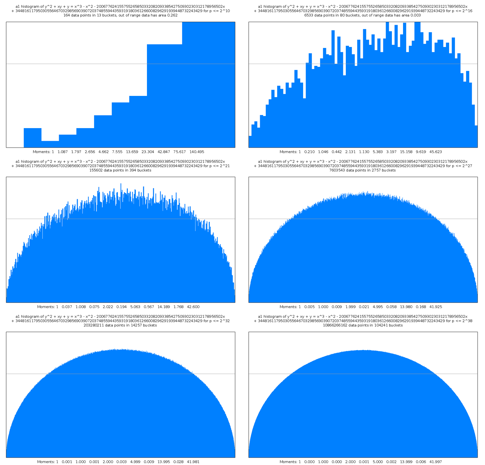
Observe that via this theorem, assuming the Birch and Swinnerton–Dyer conjecture and taking for χ\chi the character of the tautological representation of GG (seen as a subgroup of USp⁡(2​g)\mathrm{USp}(2g)), the influence of the rank of the Mordell-Weil group of AA on the rate of convergence of the measures μx\mu_{x} towards the Sato–Tate measure μ\mu becomes apparent.33 3 An effect of the rank on the convergence towards the Sato–Tate measure had been experimentally observed. On Drew Sutherland’s web page: https://math.mit.edu/~drew/g1_r28_a1f.gif,one can visualize a very asymmetric convergence towards the Sato–Tate measure in the case of Elkies’ elliptic curve (the highest rank elliptic curve known to date, of rank at least 28).
The proof of Theorem 1.3 occupies §3. It relies on work of Akbary, Ng, and Shahabi [ANS14] on the existence of a limiting distribution attached to any unitary cuspidal automorphic selfdual LL-function, and it follows the ideas that Sarnak introduced in [Sar07] (see also the discussion of Mazur–Stein [MS13, §9,§10] and Fiorilli [Fio14]) to explain the bias in the sign of the Frobenius traces of an elliptic curve in terms of the rank. Sarnak restricted his attention to elliptic curves without complex multiplication, in which case G=USp⁡(2)G=\mathrm{USp}(2) and the nontrivial irreducible representations of GG are the symmetric powers of its standard representation.

In §4, we use Theorem 1.3 to give a simple upper bound of the asymptotic L2L^{2}-norm I⁡(φ)I(\varphi). This is used in §5 to analyze the convergence rate of certain virtual characters which are of interest in the numerical calculation of Sato–Tate groups. Indeed, the usual method for such calculations is to compute approximations to the limit values of a certain set of virtual characters, for which these limit values are known to determine the Sato–Tate group. A typical example are the moments of the coefficients of the polynomial L𝔭​(A,T/|𝔭|)L_{\mathfrak{p}}(A,T/\sqrt{|{\mathfrak{p}}|}) (cf. [KS09, FKRS12]) or the so-called power sums (cf. [KS09]). Formula (1.13) can then be used to determine how fast one can expect different families of virtual characters to converge. For instance, Shieh [Shi16] experimentally observed a better convergence of the set of irreducible characters than of the moments. This is consistent with the velocities of convergence predicted by (1.13), and in fact one can view Theorem 1.3 as a theoretical justification for Shieh’s observation.

In §6 we report on some numerical experiments, carried out to test whether the predictions of convergence rate arising from Theorem 1.3 can actually be observed in concrete examples. The concrete choice of examples also reflects the goal of illustrating how the different invariants of abelian varieties (the various analytic ranks, the Frobenius–Schur index, the Sato–Tate group, etc.) affect the convergence rate.

In the spirit of Sarnak’s letter [Sar07], the results of §3 can be used to study the bias of the sign of the Frobenius trace of an abelian variety. We briefly report on this in §7.

Notations. We use |⋅||\cdot| to denote the absolute norm of ideals in rings of integers of number fields and the complex absolute value. Its use in one sense or the other should be clear from the context.

Acknowledgments. Guitart is thankful to the ESAGA group in the University of Duisburg–Essen, for their warm hospitality during his visit on the spring of 20162016 where part of this work was carried out. Thanks to Amir Akbary, Jorge Jiménez, Kiran S. Kedlaya, Victor Rotger, and Mark Watkins for suggestive remarks and helpful comments.

2. Background

In this section, we recall the results of [ANS14] that we will require in §3 and a few technical lemmas.

2.1. Limiting distributions

Let ψ:ℝ>0→ℝ\psi\colon\mathbb{R}_{>0}\rightarrow\mathbb{R} be a function admitting an expression of the form

(2.1) ψ⁡(x)=c+S⁡(x,T)+R⁡(x,T),\psi(x)=c+S(x,T)+R(x,T)\,,

for any T≥2T\geq 2, where c∈ℝc\in\mathbb{R} and:

  1. i)

    The main term S⁡(x,T)S(x,T) is of the form ℜ⁡(∑γn≤Tηn​xi​γn)\Re\left(\sum_{\gamma_{n}\leq T}\eta_{n}x^{i\gamma_{n}}\right), where {γn}n≥1⊆ℝ>0\{\gamma_{n}\}_{n\geq 1}\subseteq\mathbb{R}_{>0} is a non-decreasing sequence that tends to infinity, {ηn}n≥1⊆ℂ\{\eta_{n}\}_{n\geq 1}\subseteq\mathbb{C}, and there exists θ∈[0,3−3]\theta\in[0,3-\sqrt{3}] such that

    (2.2) ∑γn≤Tγn2​|ηn|2=O⁡(Tθ).\sum_{\gamma_{n}\leq T}\gamma_{n}^{2}|\eta_{n}|^{2}=O(T^{\theta})\,.
  2. ii)

    The error term R⁡(x,T)R(x,T) satisfies

    (2.3) limX→∞1log⁡(X)​∫2X|R⁡(x,X)|2​d​xx=0.\lim_{X\rightarrow\infty}\frac{1}{\log(X)}\int_{2}^{X}|R(x,X)|^{2}\frac{dx}{x}=0\,.

The next statement is contained in [ANS14, Cor. 1.3].

Theorem 2.1 ([ANS14]).

The function ψ\psi possesses a limiting distribution μψ\mu_{\psi} with respect to the measure d​x/xdx/x. That is, for any continuous function f:ℝ→ℝf:\mathbb{R}\rightarrow\mathbb{R} one has

(2.4) limX→∞1log⁡(X)​∫2Xf⁡(ψ⁡(x))​d​xx=∫ℝf⁡(x)​μψ​(x).\lim_{X\rightarrow\infty}\frac{1}{\log(X)}\int_{2}^{X}f(\psi(x))\frac{dx}{x}=\int_{\mathbb{R}}f(x)\mu_{\psi}(x)\,.

Moreover, the expectation and variance of μψ\mu_{\psi} are respectively

E⁡[μψ]:=∫ℝx​μψ​(x)=c,V⁡[μψ]:=∫ℝ(x−c)2​μψ​(x)=12​∑n≥1|ηn|2.\mathrm{E}[\mu_{\psi}]:=\int_{\mathbb{R}}x\mu_{\psi}(x)=c\,,\qquad\mathrm{V}[\mu_{\psi}]:=\int_{\mathbb{R}}(x-c)^{2}\mu_{\psi}(x)=\frac{1}{2}\sum_{n\geq 1}|\eta_{n}|^{2}\,.
Remark 2.2.

Let ψ\psi be as in (2.1) and let ψ′:ℝ>0→ℝ\psi^{\prime}:\mathbb{R}_{>0}\rightarrow\mathbb{R} be such that ψ⁡(x)=ψ′​(x)+Δ⁡(x)\psi(x)=\psi^{\prime}(x)+\Delta(x), where Δ⁡(x)=o⁡(1)\Delta(x)=o(1). If we write ψ′​(s)\psi^{\prime}(s) as

ψ′​(x)=c+S⁡(x,T)+R′​(x,T),\psi^{\prime}(x)=c+S(x,T)+R^{\prime}(x,T)\,,

the main term S⁡(x,T)S(x,T) and the error term R′​(x,T):=R⁡(x,T)−Δ⁡(x)R^{\prime}(x,T):=R(x,T)-\Delta(x) also satisfy (2.2) and (2.3). Indeed, this amounts to showing that

limX→∞1log⁡(X)​∫2X|Δ⁡(x)|2​d​xx=0.\lim_{X\rightarrow\infty}\frac{1}{\log(X)}\int_{2}^{X}|\Delta(x)|^{2}\frac{dx}{x}=0\,.

To prove this, let ϵ>0\epsilon>0 and note that, since Δ⁡(x)=o⁡(1)\Delta(x)=o(1), there exists Xϵ>0X_{\epsilon}>0 such that |Δ⁡(x)|2<ϵ|\Delta(x)|^{2}<\epsilon for x>Xϵx>X_{\epsilon}. Then

limX→∞1log⁡(X)​∫2X|Δ⁡(x)|2​d​xx=limX→∞1log⁡(X)​∫XϵX|Δ⁡(x)|2​d​xx≤limX→∞ϵlog⁡(X)​∫XϵXd​xx≤ϵ.\lim_{X\rightarrow\infty}\frac{1}{\log(X)}\int_{2}^{X}|\Delta(x)|^{2}\frac{dx}{x}=\lim_{X\rightarrow\infty}\frac{1}{\log(X)}\int_{X_{\epsilon}}^{X}|\Delta(x)|^{2}\frac{dx}{x}\leq\lim_{X\rightarrow\infty}\frac{\epsilon}{\log(X)}\int_{X_{\epsilon}}^{X}\frac{dx}{x}\leq\epsilon\,.

We finish this section by recording a property of the limit appearing on the left hand side of (2.4) that we will use in §3.

Lemma 2.3.

Let f:ℝ>0→ℝ≥0f\colon\mathbb{R}_{>0}\rightarrow\mathbb{R}_{\geq 0} be a locally integrable function such that

limX→∞1log⁡(X)​∫2Xf⁡(x)​𝑑x=C,\lim_{X\rightarrow\infty}\frac{1}{\log(X)}\int_{2}^{X}f(x)dx=C\,,

for some C∈ℝC\in\mathbb{R}. Let g:ℝ>0→ℝg\colon\mathbb{R}_{>0}\rightarrow\mathbb{R} be a function such that limx→∞g⁡(x)=1\displaystyle\lim_{x\rightarrow\infty}g(x)=1 and such that f​gfg is locally integrable. Then

limX→∞1log⁡(X)​∫2Xf⁡(x)​g​(x)​𝑑x=C.\displaystyle\lim_{X\rightarrow\infty}\frac{1}{\log(X)}\int_{2}^{X}f(x)g(x)dx=C\,.
Proof.

First of all, we observe that for any M≥2M\geq 2 we have that

(2.5) limX→∞1log⁡(X)​∫MXf⁡(x)​𝑑x=C.\displaystyle\lim_{X\rightarrow\infty}\frac{1}{\log(X)}\int_{M}^{X}f(x)dx=C.

Now fix ϵ>0\epsilon>0 and let XϵX_{\epsilon} be such that g⁡(x)g(x) belongs to the interval [1−ϵ,1+ϵ][1-\epsilon,1+\epsilon] for all x≥Xϵx\geq X_{\epsilon}. Then, for any X≥XϵX\geq X_{\epsilon} we have

1log⁡(X)​∫2Xf⁡(x)​g​(x)​𝑑x=\displaystyle\frac{1}{\log(X)}\int_{2}^{X}f(x)g(x)dx= 1log⁡(X)​∫2Xϵf⁡(x)​g​(x)​𝑑x+1log⁡(X)​∫XϵXf⁡(x)​g​(x)​𝑑x\displaystyle\frac{1}{\log(X)}\int_{2}^{X_{\epsilon}}f(x)g(x)dx+\frac{1}{\log(X)}\int_{X_{\epsilon}}^{X}f(x)g(x)dx
≤\displaystyle\leq 1log⁡(X)​∫2Xϵf⁡(x)​g​(x)​𝑑x+(1+ϵ)log⁡(X)​∫XϵXf⁡(x)​𝑑x.\displaystyle\frac{1}{\log(X)}\int_{2}^{X_{\epsilon}}f(x)g(x)dx+\frac{(1+\epsilon)}{\log(X)}\int_{X_{\epsilon}}^{X}f(x)dx.

Now, by (2.5) for XX sufficiently large we will have that

1log⁡(X)​∫XϵXf⁡(x)​𝑑x≤C+ϵ.\displaystyle\frac{1}{\log(X)}\int_{X_{\epsilon}}^{X}f(x)dx\leq C+\epsilon\,.

Also, for XX large enough

1log⁡(X)​∫2Xϵf⁡(x)​g​(x)​𝑑x≤ϵ.\displaystyle\frac{1}{\log(X)}\int_{2}^{X_{\epsilon}}f(x)g(x)dx\leq\epsilon\,.

Therefore, we see that for XX large enough we have that

1log⁡(X)​∫2Xf⁡(x)​g​(x)​𝑑x≤ϵ+(1+ϵ)​(C+ϵ)=C+ϵ⁡(2+C+ϵ).\displaystyle\frac{1}{\log(X)}\int_{2}^{X}f(x)g(x)dx\leq\epsilon+(1+\epsilon)(C+\epsilon)=C+\epsilon(2+C+\epsilon).

Now, mutatis mutandis one can also show that for XX large enough one has

1log⁡X​∫2Xf⁡(x)​g​(x)​𝑑x≥C−ϵ⁡(2+C−ϵ)\displaystyle\frac{1}{\log X}\int_{2}^{X}f(x)g(x)dx\geq C-\epsilon(2+C-\epsilon)

and we see that the limit when X→∞X\rightarrow\infty is also CC. ∎

2.2. Limiting distributions of automorphic LL-functions

Let π\pi be an irreducible unitary cuspidal automorphic representation of GLr⁡(𝔸ℚ)\operatorname{GL}_{r}(\mathbb{A}_{\mathbb{Q}}), for some r≥1r\geq 1, and let L⁡(π,s)L(\pi,s) denote the automorphic LL-function attached to π\pi. Suppose that L⁡(π,s)≠ζ⁡(s−i​τ0)L(\pi,s)\not=\zeta(s-i\tau_{0}) for any τ0∈ℝ\tau_{0}\in\mathbb{R}, where ζ\zeta denotes the Riemann Zeta function. For n≥1n\geq 1, define the coefficients Λπ​(n)\Lambda_{\pi}(n), by prescribing an equality of Dirichlet series

(2.6) −L​(π,s)′L⁡(π,s)=:∑n≥1Λπ​(n)​n−s,-\frac{L(\pi,s)^{\prime}}{L(\pi,s)}=:\sum_{n\geq 1}\Lambda_{\pi}(n)n^{-s}\,,

and, for x>0x>0, define the function

(2.7) ψ⁡(π,x):=1x​∑n≤xΛπ​(n).\displaystyle\psi(\pi,x):=\frac{1}{\sqrt{x}}\sum_{n\leq x}\Lambda_{\pi}(n)\,.

The following is [ANS14, Prop. 4.2].

Theorem 2.4.

Under the Riemann Hypothesis for L⁡(π,s)L(\pi,s), for any x>0x>0 and T≥2T\geq 2, we have

(2.8) ψ⁡(π,x)=−2​rπ−∑0<|γπ|≤Txi​γπ1/2+i​γπ+Rπ​(x,T).\displaystyle\psi(\pi,x)=-2r_{\pi}-\sum_{0<|\gamma_{\pi}|\leq T}\frac{x^{i\gamma_{\pi}}}{1/2+i\gamma_{\pi}}+R_{\pi}(x,T)\,.

Here, rπr_{\pi} denotes the order of the zero of L⁡(π,s)L(\pi,s) at s=1/2s=1/2, γπ\gamma_{\pi} runs over the non-zero imaginary parts of absolute value up to TT of the zeros of L⁡(π,s)L(\pi,s) on the critical line, and the error term Rπ​(x,T)R_{\pi}(x,T) satisfies

Rπ​(x,T)=O⁡(x1/2+β​log2⁡(x)T+xβ−1/2​log⁡(x)+x1/2​log2⁡(T)T​log⁡(x)+x1/2​log⁡(T)T),\displaystyle R_{\pi}(x,T)=O\left(\frac{x^{1/2+\beta}\log^{2}(x)}{T}+x^{\beta-1/2}\log(x)+\frac{x^{1/2}\log^{2}(T)}{T\log(x)}+\frac{x^{1/2}\log(T)}{T}\right),

for some β∈[0,1/2)\beta\in[0,1/2).

Remark 2.5.

By combining Theorems 2.4 and 2.1, one obtains as in [ANS14, §4.1] that if π\pi is selfdual44 4 We alert the reader that the selfduality condition on π\pi does not appear in the statement of [ANS14, Cor. 1.5], although it is used in the proof (see the last display in page 767767 of loc. cit.)., then ψ⁡(π,x)\psi(\pi,x) has a limiting distribution with respect to the measure d​x/xdx/x (see [ANS14, Cor. 1.5]). Indeed, if π\pi is selfdual the zeros of L⁡(π,s)L(\pi,s) come in conjugate pairs, and by pairing them one sees that ψ⁡(π,x)\psi(\pi,x) can be written as in (2.1) in such a way that Rπ​(x,T)R_{\pi}(x,T) satisfies (2.3) and that, if {γn}n≥1\{\gamma_{n}\}_{n\geq 1} is an ordering by size of the positive imaginary parts of the zeros of L⁡(π,s)L(\pi,s) on the critical line, then (2.2) is satisfied with ηn:=−2/(1/2+iγn)\eta_{n}:=-2/(1/2+i\gamma_{n}) and θ:=β\theta:=\beta. We will apply a similar argument to c​ψ​(π,x)+c¯​ψ​(π∨,x)c\psi(\pi,x)+\bar{c}\psi(\pi^{\vee},x), with c∈ℂc\in\mathbb{C}, if π\pi is not selfdual (see Corollary 3.3 below).

3. Proof of Theorem 1.3

Resume the notations of §1. The first step towards the proof of Theorem 1.3 is to consider the case of a nontrivial irreducible character χ\chi of GG. For x>0x>0, define the function

ψ⁡(χ,x):=log⁡(x)x​∑|𝔭|≤xχ⁡(y𝔭).\psi(\chi,x):=\frac{\log(x)}{\sqrt{x}}\sum_{|{\mathfrak{p}}|\leq x}\chi(y_{\mathfrak{p}})\,.
Proposition 3.1.

Under Assumption 1.1, for a nontrivial irreducible character χ\chi of GG and for any x>0x>0 and T≥2T\geq 2, we have that

(3.1) ψ⁡(χ,x)=−2​rχ−uχ−∑0<|γχ|≤Txi​γχ1/2+i​γχ+R⁡(x,T),\displaystyle\psi(\chi,x)=-2r_{\chi}-u_{\chi}-\sum_{0<|\gamma_{\chi}|\leq T}\frac{x^{i\gamma_{\chi}}}{1/2+i\gamma_{\chi}}+R(x,T)\,,

where rχr_{\chi}, uχu_{\chi} are as in the statement of Theorem 1.3, γχ\gamma_{\chi} runs over the non-zero imaginary parts of absolute value up to TT of the zeros of L⁡(χ,s)L(\chi,s) on the critical line, and the error term R⁡(x,T)R(x,T) satisfies (2.3).

Proof.

Let ϱ\varrho be an irreducible representation of GG of character χ\chi, and let dχd_{\chi} denote the degree of ϱ\varrho. For n≥1n\geq 1, define the von-Mangold function Λχ​(n)\Lambda_{\chi}(n) by prescribing an equality of Dirichlet series

(3.2) −L​(χ,s)′L⁡(χ,s)=:∑n≥1Λχ​(n)​n−s.-\frac{L(\chi,s)^{\prime}}{L(\chi,s)}=:\sum_{n\geq 1}\Lambda_{\chi}(n)n^{-s}\,.

For a prime 𝔭{\mathfrak{p}} of kk, let α𝔭,1,…,α𝔭,dχ​(𝔭)\alpha_{{\mathfrak{p}},1},\dots,\alpha_{{\mathfrak{p}},d_{\chi}({\mathfrak{p}})} denote the recyprocal roots of L𝔭​(χ,T)L_{\mathfrak{p}}(\chi,T). Taking the logarithmic derivative in (1.9), we find that

(3.3) −L​(χ,s)′L⁡(χ,s)=∑𝔭∑j=1dχ​(𝔭)∑r≥1log⁡(|𝔭|)​α𝔭,jr|𝔭|r​s=∑r≥1∑𝔭log⁡(|𝔭|)​(∑j=1dχ​(𝔭)α𝔭,jr)​|𝔭|−r​s.\displaystyle-\frac{L(\chi,s)^{\prime}}{L(\chi,s)}=\sum_{{\mathfrak{p}}}\sum_{j=1}^{d_{\chi}(\mathfrak{p})}\sum_{r\geq 1}\frac{\log(|{\mathfrak{p}}|)\alpha_{\mathfrak{p},j}^{r}}{|{\mathfrak{p}}|^{rs}}=\sum_{r\geq 1}\sum_{{\mathfrak{p}}}\log(|{\mathfrak{p}}|)\big(\sum_{j=1}^{d_{\chi}(\mathfrak{p})}\alpha_{\mathfrak{p},j}^{r}\big)|{\mathfrak{p}}|^{-rs}\,.

For r≥1r\geq 1, define55 5 Note that we are using the same notation Λχ\Lambda_{\chi} to denote two different functions; since one is a function of the positive integers and the other is a function of the ideals of kk, their argument makes clear which one we refer to (when k=ℚk=\mathbb{Q} the two functions coincide).

Λχ​(𝔭r):=log⁡(|𝔭|)​(∑j=1dχ​(𝔭)α𝔭,jr).\Lambda_{\chi}({\mathfrak{p}}^{r}):=\log(|{\mathfrak{p}}|)\big(\sum_{j=1}^{d_{\chi}(\mathfrak{p})}\alpha_{\mathfrak{p},j}^{r}\big)\,.

Note that, if 𝔭∈P{\mathfrak{p}}\in P, then α𝔭,1,…,α𝔭,dχ​(𝔭)\alpha_{{\mathfrak{p}},1},\dots,\alpha_{{\mathfrak{p}},d_{\chi}({\mathfrak{p}})} are the eigenvalues of ϱ⁡(y𝔭)\varrho(y_{\mathfrak{p}}) and thus Λχ​(𝔭r)=log⁡(|𝔭|)​χ​(y𝔭r)\Lambda_{\chi}({\mathfrak{p}}^{r})=\log(|{\mathfrak{p}}|)\chi(y_{\mathfrak{p}}^{r}). Observe also that we similarly find that

−LP​(χ,s)′LP​(χ,s)=∑r≥1∑𝔭∈PΛχ​(𝔭r)​|𝔭|−r​s,-\frac{L^{P}(\chi,s)^{\prime}}{L^{P}(\chi,s)}=\sum_{r\geq 1}\sum_{{\mathfrak{p}}\in P}\Lambda_{\chi}({\mathfrak{p}}^{r})|{\mathfrak{p}}|^{-rs}\,,

For x>0x>0, define the function

(3.4) ψ1​(χ,x):=1x​∑n≤xΛχ​(n)=1x​∑r≥1∑|𝔭|r≤xΛχ​(𝔭r),\psi_{1}(\chi,x):=\frac{1}{\sqrt{x}}\sum_{n\leq x}\Lambda_{\chi}(n)=\frac{1}{\sqrt{x}}\sum_{r\geq 1}\sum_{|{\mathfrak{p}}|^{r}\leq x}\Lambda_{\chi}({\mathfrak{p}}^{r})\,,

where the second equality follows from compairing (3.3) and (3.2). Under Assumption 1.1, there is an irreducible unitary cuspidal representation π\pi of GLdχ[k:ℚ](𝔸ℚ)\operatorname{GL}_{d_{\chi}[k:\mathbb{Q}]}(\mathbb{A}_{\mathbb{Q}}) such that ψ1​(χ,x)\psi_{1}(\chi,x) coincides with ψ⁡(π,x)\psi(\pi,x), as defined in (2.7) (note that L⁡(π,s)L(\pi,s) is not of the form ζ⁡(s−i​τ0)\zeta(s-i\tau_{0}) since χ\chi is nontrivial). Then, by Theorem 2.4 we can write

ψ1​(χ,x)=c1+S1​(x,T)+R1​(x,T),\psi_{1}(\chi,x)=c_{1}+S_{1}(x,T)+R_{1}(x,T)\,,

where c1:=−2​rχc_{1}:=-2r_{\chi}, S1(T):=−∑0<|γχ|≤Txi​γχ1/2+i​γχS_{1}(T):=-\sum_{0<|\gamma_{\chi}|\leq T}\frac{x^{i\gamma_{\chi}}}{1/2+i\gamma_{\chi}} and R1​(x,T)R_{1}(x,T) satisfies (2.3). Define

ψ2​(χ,x):=1x​∑|𝔭|≤xΛχ​(𝔭),Δ1​(x):=1x​(∑|𝔭|≤x1/2Λχ​(𝔭2)+∑k≥3∑|𝔭|≤x1/kΛχ​(𝔭k)),\psi_{2}(\chi,x):=\frac{1}{\sqrt{x}}\sum_{|{\mathfrak{p}}|\leq x}\Lambda_{\chi}({\mathfrak{p}})\,,\qquad\Delta_{1}(x):=\frac{1}{\sqrt{x}}\left(\sum_{|{\mathfrak{p}}|\leq x^{1/2}}\Lambda_{\chi}({\mathfrak{p}}^{2})+\sum_{k\geq 3}\sum_{|{\mathfrak{p}}|\leq x^{1/k}}\Lambda_{\chi}({\mathfrak{p}}^{k})\right)\,,

so that ψ1​(χ,x)=ψ2​(χ,x)+Δ1​(x)\psi_{1}(\chi,x)=\psi_{2}(\chi,x)+\Delta_{1}(x). We proceed to study the size of Δ1​(x)\Delta_{1}(x). On the one hand, we have

∑|𝔭|≤x1/kΛχ(𝔭k)≤dχ∑|𝔭|≤x1/klog(|𝔭|)≤dχ[k:ℚ]x1/klog(x).\displaystyle\sum_{|{\mathfrak{p}}|\leq x^{1/k}}\Lambda_{\chi}({\mathfrak{p}}^{k})\leq d_{\chi}\sum_{|{\mathfrak{p}}|\leq x^{1/k}}\log(|{\mathfrak{p}}|)\leq d_{\chi}[k:\mathbb{Q}]x^{1/k}\log(x)\,.

Since there is no prime ideal 𝔭{\mathfrak{p}} of kk such that |𝔭|≤x1/k|{\mathfrak{p}}|\leq x^{1/k} when k>log2⁡(x)k>\log_{2}(x), the sum indexed by kk in Δ1​(x)\Delta_{1}(x) has at most O⁡(log⁡(x))O(\log(x)) summands. Therefore the right most summand in Δ1​(x)\Delta_{1}(x) is O⁡(x1/3​log2⁡(x))O(x^{1/3}\log^{2}(x)). On the other hand, (1.7) says that

∑|𝔭|≤x1/2Λχ(𝔭2)=δ(χ(⋅2))x+o(x),\sum_{|{\mathfrak{p}}|\leq x^{1/2}}\Lambda_{\chi}({\mathfrak{p}}^{2})=\delta(\chi(\cdot^{2}))\sqrt{x}+o(\sqrt{x}),

where χ(⋅2)\chi(\cdot^{2}) denotes the central function g↦χ⁡(g2)g\mapsto\chi(g^{2}). Note that the multiplicity δ(χ(⋅2))\delta(\chi(\cdot^{2})) equals uχ:=∫Gχ⁡(g2)​μG​(g)u_{\chi}:=\int_{G}\chi(g^{2})\mu_{G}(g), the so-called Frobenius–Schur index of χ\chi. It is known that uχ=0u_{\chi}=0 if χ\chi takes some complex nonreal value, uχ=1u_{\chi}=1 if χ\chi is attached to a representation realizable over ℝ\mathbb{R}, and uχ=−1u_{\chi}=-1 if χ\chi is attached to a quaternionic representation (i.e., a representation that is not realizable over ℝ\mathbb{R}, even if its character takes values in ℝ\mathbb{R}). We deduce that

ψ2​(χ,x)=ψ1​(χ,x)−uχ+o⁡(1),\psi_{2}(\chi,x)=\psi_{1}(\chi,x)-u_{\chi}+o(1)\,,

and by Remark 2.2, we deduce that

(3.5) ψ2​(χ,x)=c2+S2​(x,T)+R2​(x,T),\psi_{2}(\chi,x)=c_{2}+S_{2}(x,T)+R_{2}(x,T)\,,

where c2:=c1−uχc_{2}:=c_{1}-u_{\chi}, S2​(x,T):=S1​(x,T)S_{2}(x,T):=S_{1}(x,T), and R2​(x,T)R_{2}(x,T) satisfies (2.3). For x>0x>0, define the function

ψ3​(χ,x):=1x​∑|𝔭|≤x,𝔭∈PΛχ​(𝔭),\psi_{3}(\chi,x):=\frac{1}{\sqrt{x}}\sum_{|{\mathfrak{p}}|\leq x,\mathfrak{p}\in P}\Lambda_{\chi}({\mathfrak{p}})\,,

so that we have that

ψ2​(χ,x)=ψ3​(χ,x)+Δ2​(x),whereΔ2​(x):=1x​∑𝔭|𝔑Λχ​(𝔭).\psi_{2}(\chi,x)=\psi_{3}(\chi,x)+\Delta_{2}(x)\,,\qquad\text{where}\qquad\Delta_{2}(x):=\frac{1}{\sqrt{x}}\sum_{\mathfrak{p}|\mathfrak{N}}\Lambda_{\chi}({\mathfrak{p}})\,.

Provided that there is only a finite number of primes dividing 𝔑\mathfrak{N}, we have that Δ2​(x)=o​(1)\Delta_{2}(x)=o(1). But, by the Abel summation trick (see Lemma 3.2 below), we have that ψ3​(χ,x)=ψ⁡(χ,x)+o⁡(1)\psi_{3}(\chi,x)=\psi(\chi,x)+o(1). It follows from Remark 2.2, that ψ⁡(χ,x)\psi(\chi,x) admits an expression of the form ψ⁡(χ,x)=c+S⁡(x,T)+R⁡(x,T)\psi(\chi,x)=c+S(x,T)+R(x,T), with c=c2c=c_{2}, S⁡(x,T):=S2​(x,T)S(x,T):=S_{2}(x,T), and R⁡(x,T)R(x,T) satisfies (2.3).

∎

At the end of the previous proof we have applied the Abel summation trick. Following the lines of reasoning of [RS94, Lemma 2.1], we give the argument involved in gory detail.

Lemma 3.2.

For a nontrivial character χ\chi of GG, we have

(3.6) ∑|𝔭|≤xlog⁡(|𝔭|)​χ​(y𝔭)=log⁡(x)​∑|𝔭|≤xχ⁡(y𝔭)+o⁡(x).\displaystyle\sum_{|{\mathfrak{p}}|\leq x}\log(|{\mathfrak{p}}|)\chi(y_{\mathfrak{p}})=\log(x)\sum_{|{\mathfrak{p}}|\leq x}\chi(y_{\mathfrak{p}})+o(\sqrt{x})\,.
Proof.

Let us write

ϑ⁡(x):=x⋅ψ3​(χ,x)=∑|𝔭|≤xlog⁡(|𝔭|)​χ​(y𝔭).\vartheta(x):=\sqrt{x}\cdot\psi_{3}(\chi,x)=\sum_{|{\mathfrak{p}}|\leq x}\log(|{\mathfrak{p}}|)\chi(y_{\mathfrak{p}})\,.

Applying summation by parts66 6 We apply the formula of [IK04, Chap. I, §1.5], with f⁡(pr)=∑|𝔭|=prlog⁡(|𝔭|)​χ​(y𝔭)f(p^{r})=\sum_{|{\mathfrak{p}}|=p^{r}}\log(|{\mathfrak{p}}|)\chi(y_{\mathfrak{p}}) (and f⁡(n)=0f(n)=0 if nn is not a prime power) and g⁡(x)=1/log⁡(x)g(x)=1/\log(x)., we have

(3.7) ∑|𝔭|≤xχ⁡(y𝔭)=ϑ⁡(x)log⁡(x)+∫2xϑ⁡(t)t​log2​(t)​𝑑t.\displaystyle\sum_{|{\mathfrak{p}}|\leq x}\chi(y_{\mathfrak{p}})=\frac{\vartheta(x)}{\log(x)}+\int_{2}^{x}\frac{\vartheta(t)}{t\log^{2}(t)}dt\,.

Then, integrating (3.5) times x\sqrt{x}, letting TT tend to infinity, and using that β<1/2\beta<1/2 we obtain

(3.8) G⁡(x):=∫2xϑ⁡(t)​𝑑t=23​(−2​rχ−uχ)​x3/2−∑γχ≠0x32+i​γχ(12+i​γχ)​(32+i​γχ)+o⁡(x3/2).\displaystyle G(x):=\int_{2}^{x}\vartheta(t)dt=\frac{2}{3}(-2r_{\chi}-u_{\chi})x^{3/2}-\sum_{\gamma_{\chi}\neq 0}\frac{x^{\frac{3}{2}+i\gamma_{\chi}}}{(\frac{1}{2}+i\gamma_{\chi})(\frac{3}{2}+i\gamma_{\chi})}+o(x^{3/2}).

As in the proof of [RS94, Lemma 2.1], here we are using the fact that the series over γχ\gamma_{\chi} converges absolutely. This follows from the asymptotic formula for the number N⁡(T)N(T) of zeros on the critical line with imaginary part of absolute value ≤T\leq T for automorphic LL-functions, as in for example [IK04, Theorem 5.8]. It follows that G⁡(x)=O⁡(x3/2)G(x)=O(x^{3/2}).

Integrating by parts the rightmost integral in (3.7), we obtain

∫2xϑ⁡(t)t​log2​(t)​𝑑t=G⁡(x)x​log2​x+∫2xG⁡(t)​log⁡(t)+2t2​log3​(t)​𝑑t=O⁡(xlog2⁡(x))+O⁡(∫2xd​tt⋅log2⁡(t)).\int_{2}^{x}\frac{\vartheta(t)}{t\log^{2}(t)}dt=\frac{G(x)}{x\log^{2}x}+\int_{2}^{x}G(t)\frac{\log(t)+2}{t^{2}\log^{3}(t)}dt=O\left(\frac{\sqrt{x}}{\log^{2}(x)}\right)+O\left(\int_{2}^{x}\frac{dt}{\sqrt{t}\cdot\log^{2}(t)}\right)\,.

Both OO-terms in the above expression are o⁡(xlog⁡x)o\left(\frac{\sqrt{x}}{\log x}\right) (the first by trivial reasons and the second, by l’Hôpital, for example). We conclude that

(3.9) ∑|𝔭|≤xχ⁡(y𝔭)=ϑ⁡(x)log⁡(x)+o⁡(xlog⁡(x)),\displaystyle\sum_{|{\mathfrak{p}}|\leq x}\chi(y_{\mathfrak{p}})=\frac{\vartheta(x)}{\log(x)}+o\left(\frac{\sqrt{x}}{\log(x)}\right),

and this implies the lemma. ∎

Corollary 3.3.

With the notation and assumptions as in Proposition 3.1 and for cχ∈ℂc_{\chi}\in\mathbb{C} we have that

cχ​ψ​(χ,x)+c¯χ​ψ​(χ¯,x)=−2​(cχ​rχ+c¯χ​rχ¯)−(cχ​uχ+c¯χ​uχ¯)+S⁡(x,T)+R⁡(x,T),\displaystyle c_{\chi}\psi(\chi,x)+\bar{c}_{\chi}\psi(\bar{\chi},x)=-2(c_{\chi}r_{\chi}+\bar{c}_{\chi}r_{\bar{\chi}})-(c_{\chi}u_{\chi}+\bar{c}_{\chi}u_{\bar{\chi}})+S(x,T)+R(x,T),

where S⁡(x,T)S(x,T) and R⁡(x,T)R(x,T) are as in (2.1), R⁡(x,T)R(x,T) satisfies (2.3), and S⁡(x,T)S(x,T) satisfies (2.2) with {γn}n≥1\{\gamma_{n}\}_{n\geq 1} being the positive imaginary parts of the zeros of L⁡(χ,s)L(\chi,s) and L⁡(χ¯,s)L(\bar{\chi},s), ηn:=−2​cχ1/2+i​γn\eta_{n}:=\frac{-2c_{\chi}}{1/2+i\gamma_{n}} if γn\gamma_{n} corresponds a zero of L⁡(χ,s)L(\chi,s), ηn:=−2​c¯χ1/2+i​γn\eta_{n}:=\frac{-2\bar{c}_{\chi}}{1/2+i\gamma_{n}} if γn\gamma_{n} corresponds to a zero of L⁡(χ¯,s)L(\bar{\chi},s), and θ=1/2\theta=1/2.

Proof.

This follows at once by adding the expressions for cχ​ψ​(χ,x)c_{\chi}\psi(\chi,x) and c¯χ​ψ​(χ¯,x)\bar{c}_{\chi}\psi(\bar{\chi},x) given in (3.1) and pairing each zero 12+i​γχ\frac{1}{2}+i\gamma_{\chi} of L⁡(χ,s)L(\chi,s) having γχ>0\gamma_{\chi}>0 with its conjugate, which is a zero of L⁡(χ¯,s)L(\bar{\chi},s) (and, similarly, pairing each zero 12+i​γχ¯\frac{1}{2}+i\gamma_{\bar{\chi}} of L⁡(χ¯,s)L(\bar{\chi},s) having γχ¯>0\gamma_{\bar{\chi}}>0 with its conjugate, which is a zero of L⁡(χ,s)L(\chi,s)). ∎

Remark 3.4.

Observe that, in fact, rχ=rχ¯r_{\chi}=r_{\bar{\chi}} and uχ=uχ¯u_{\chi}=u_{\bar{\chi}}.

Theorem 3.5.

Under Assumption 1.1, for every virtual character of the form φ=∑χ≠1cχ​χ\varphi=\sum_{\chi\not=1}c_{\chi}\chi, where cχ∈ℂc_{\chi}\in\mathbb{C} and χ\chi runs over the irreducible nontrivial characters of GG, one has

(3.10) limX→∞1log⁡X∫2Xψ(φ,x)d​xx=−∑χcχ(2rχ+uχ).\lim_{X\rightarrow\infty}\frac{1}{\log X}\int_{2}^{X}\psi(\varphi,x)\frac{dx}{x}=-\sum_{\chi}c_{\chi}(2r_{\chi}+u_{\chi}).
(3.11) limX→∞1log⁡X​∫2X|ψ⁡(φ,x)|2​d​xx=|∑χcχ​(2​rχ+uχ)|2+∑χ∑γχ≠0|cχ|21/4+γχ2,\lim_{X\rightarrow\infty}\frac{1}{\log X}\int_{2}^{X}|\psi(\varphi,x)|^{2}\frac{dx}{x}=\big|\sum_{\chi}c_{\chi}(2r_{\chi}+u_{\chi})\big|^{2}+\sum_{\chi}\sum_{\gamma_{\chi}\neq 0}\frac{|c_{\chi}|^{2}}{1/4+\gamma_{\chi}^{2}}\,,

where ψ⁡(φ,x):=∑χcχ​ψ​(χ,x)\psi(\varphi,x):=\sum_{\chi}c_{\chi}\psi(\chi,x) and rχr_{\chi}, uχu_{\chi}, and γχ\gamma_{\chi} are as in the statement of Theorem 1.3.

Proof.

We begin by assuming that φ\varphi is selfdual. We say that a virtual character φ=∑χcχ​χ\varphi=\sum_{\chi}c_{\chi}\chi, where cχ∈ℂc_{\chi}\in\mathbb{C} and χ\chi runs over irreducible characters of GG, is selfdual if77 7 Observe that this condition is trivially satisfied if χ\chi is selfdual, since χ≃χ¯\chi\simeq\bar{\chi} in this case. cχ=c¯χ¯c_{\chi}=\bar{c}_{\bar{\chi}}, where χ¯\bar{\chi} denotes the dual (or complex conjugate) of χ\chi.

By Corollary 3.3 and Theorem 2.1, we have that for each of the irreducible constituents χ\chi of φ\varphi, the function cχ​ψ​(χ,x)+cχ¯​ψ​(χ¯,x)c_{\chi}\psi(\chi,x)+c_{\bar{\chi}}\psi(\bar{\chi},x) admits a limiting distribution μχ\mu_{\chi} with

E⁡[μχ]=−2​(cχ​rχ+cχ¯​rχ¯)−(cχ​uχ+cχ¯​uχ¯)\mathrm{E}[\mu_{\chi}]=-2(c_{\chi}r_{\chi}+c_{\bar{\chi}}r_{\bar{\chi}})-(c_{\chi}u_{\chi}+c_{\bar{\chi}}u_{\bar{\chi}})
V⁡[μχ]=∑γχ>02​|cχ|21/4+γχ2+∑γχ¯>02​|c¯χ|21/4+γχ¯2.\mathrm{V}[\mu_{\chi}]=\sum_{\gamma_{\chi}>0}\frac{{2}|c_{\chi}|^{2}}{1/4+\gamma_{\chi}^{2}}+\sum_{\gamma_{\bar{\chi}}>0}\frac{{2}|\bar{c}_{\chi}|^{2}}{1/4+\gamma_{\bar{\chi}}^{2}}.

By additivity and the fact that φ\varphi is selfdual, it follows again from Theorem 2.1 that the function ψ⁡(φ,x)\psi(\varphi,x) admits a limiting distribution μφ\mu_{\varphi} with

E[μφ]=−∑χcχ(2rχ+uχ),V[μφ]=2∑χ∑γχ>0|cχ|21/4+γχ2.\mathrm{E}[\mu_{\varphi}]=-\sum_{\chi}c_{\chi}(2r_{\chi}+u_{\chi})\,,\qquad\mathrm{V}[\mu_{\varphi}]={2}\sum_{\chi}\sum_{\gamma_{\chi}>0}\frac{|c_{\chi}|^{2}}{1/4+\gamma_{\chi}^{2}}\,.

Now (3.10) is a restatement of the above formula for the mean and (3.11) is obtained as

limX→∞1log⁡(X)​∫2Xψ​(φ,x)2​d​xx=E​[μφ]2+V⁡[μφ]=(∑χcχ​(2​rχ+uχ))2+2​∑χ∑γχ>0|cχ|21/4+γχ2.\lim_{X\rightarrow\infty}\frac{1}{\log(X)}\int_{2}^{X}\psi(\varphi,x)^{2}\frac{dx}{x}=\mathrm{E}[\mu_{\varphi}]^{2}+\mathrm{V}[\mu_{\varphi}]=\left(\sum_{\chi}c_{\chi}(2r_{\chi}+u_{\chi})\right)^{2}+{2}\sum_{\chi}\sum_{\gamma_{\chi}>0}\frac{|c_{\chi}|^{2}}{1/4+\gamma_{\chi}^{2}}\,.

Now consider the case where φ\varphi is not selfdual. Then we can write φ=φR+i​φI\varphi=\varphi_{R}+i\varphi_{I}, where

φR:=φ+φ¯2, and φI:=φ−φ¯2​i.\varphi_{R}:=\frac{\varphi+\bar{\varphi}}{2},\ \ \text{ and }\ \ \varphi_{I}:=\frac{\varphi-\bar{\varphi}}{2i}.

One easily checks that φR\varphi_{R} and φI\varphi_{I} are virtual selfdual characters, and this immediately implies (3.10). As for (3.11), note that one has

|ψ⁡(φ,x)|2=ψ​(φR,x)2+ψ​(φI,x)2.\displaystyle|\psi(\varphi,x)|^{2}=\psi(\varphi_{R},x)^{2}+\psi(\varphi_{I},x)^{2}.

Applying the previous case to both terms, and noting that

φR=∑χcχ+c¯χ¯2​χ,φI=∑χcχ−c¯χ¯2​i​χ,\displaystyle\varphi_{R}=\sum_{\chi}\frac{c_{\chi}+\bar{c}_{\bar{\chi}}}{2}\chi,\ \ \varphi_{I}=\sum_{\chi}\frac{c_{\chi}-\bar{c}_{\bar{\chi}}}{2i}\chi,

we get

limX→∞1log⁡X​∫2X|ψ⁡(φ,x)|2​d​xx=(∑χcχ+c¯χ¯2​(2​rχ+uχ))2+12​∑χ∑γχ>0|cχ+c¯χ¯|21/4+γχ2\displaystyle\lim_{X\rightarrow\infty}\frac{1}{\log X}\int_{2}^{X}|\psi(\varphi,x)|^{2}\frac{dx}{x}=\big(\sum_{\chi}\frac{c_{\chi}+\bar{c}_{\bar{\chi}}}{2}(2r_{\chi}+u_{\chi})\big)^{2}+\frac{1}{2}\sum_{\chi}\sum_{\gamma_{\chi}>0}\frac{|c_{\chi}+\bar{c}_{\bar{\chi}}|^{2}}{1/4+\gamma_{\chi}^{2}}
−(∑χcχ−c¯χ¯2​(2​rχ+uχ))2+12​∑χ∑γχ>0|cχ−c¯χ¯|21/4+γχ2.\displaystyle-\big(\sum_{\chi}\frac{c_{\chi}-\bar{c}_{\bar{\chi}}}{2}(2r_{\chi}+u_{\chi})\big)^{2}+\frac{1}{2}\sum_{\chi}\sum_{\gamma_{\chi}>0}\frac{|c_{\chi}-\bar{c}_{\bar{\chi}}|^{2}}{1/4+\gamma_{\chi}^{2}}.

The first and third term in the right hand side of the above expression add up to

|∑χcχ​(2​rχ+uχ)|2,\big|\sum_{\chi}c_{\chi}(2r_{\chi}+u_{\chi})\big|^{2},

and the second and fourth, applying parallelogram’s law, add up to

∑χ∑γχ>0|cχ|214+γχ2+∑χ∑γχ>0|cχ¯|214+γχ2;\displaystyle\sum_{\chi}\sum_{\gamma_{\chi}>0}\frac{|c_{\chi}|^{2}}{\frac{1}{4}+\gamma_{\chi}^{2}}+\sum_{\chi}\sum_{\gamma_{\chi}>0}\frac{|c_{\bar{\chi}}|^{2}}{\frac{1}{4}+\gamma_{\chi}^{2}};

Now using that

∑χ∑γχ>0|cχ¯|214+γχ2=∑χ∑γχ¯>0|cχ|214+γχ¯2=∑χ∑γχ<0|cχ|214+γχ2\displaystyle\sum_{\chi}\sum_{\gamma_{\chi}>0}\frac{|c_{\bar{\chi}}|^{2}}{\frac{1}{4}+\gamma_{\chi}^{2}}=\sum_{\chi}\sum_{\gamma_{\bar{\chi}>0}}\frac{|c_{\chi}|^{2}}{\frac{1}{4}+\gamma_{\bar{\chi}}^{2}}=\sum_{\chi}\sum_{\gamma_{\chi}<0}\frac{|c_{\chi}|^{2}}{\frac{1}{4}+\gamma_{\chi}^{2}}

we conclude the proof. ∎

We can now prove Theorem 1.3. Indeed, it follows from (3.11), Lemma 2.3 and the fact that

|ψ⁡(φ,x)|2x∼|δ⁡(φ,x)|2asx→∞.\frac{|\psi(\varphi,x)|^{2}}{x}\sim|\delta(\varphi,x)|^{2}\qquad\text{as}\qquad x\rightarrow\infty\,.

4. An upper bound for the asymptotic L2L^{2}-norm

In this section we elaborate on Theorem 1.3 to obtain an explicit and simple upper bound for the asymptotic L2L^{2}-norm, which we will use in the applications discussed in §5. Since in §5 we will only be interested in selfdual virtual characters with integral coefficients, from now on we will make the simplifying assumption that φ∈⨁χ≠1ℤ⋅χ\varphi\in\bigoplus_{\chi\neq 1}\mathbb{Z}\cdot\chi and cχ=cχ¯c_{\chi}=c_{\bar{\chi}}. We remark that all the constants appearing in this section are absolute and effectively computable.

We will need the following consequence of Assumption 1.1 (1), which we record as a remark for future reference.

Remark 4.1.

If χ\chi is an irreducible nontrivial character of GG, as a consequence of the fact that L⁡(χ,s)L(\chi,s) is automorphic, we have that (see [IK04, §5]) there exist a positive integer NχN_{\chi} (the so-called absolute conductor of χ\chi) and complex numbers κχ,j\kappa_{\chi,j} with ℜ⁡(κχ,j)>−1\Re(\kappa_{\chi,j})>-1 for j=1,…,dχj=1,\dots,d_{\chi} (the so-called local parameters at infinity of L⁡(χ,s)L(\chi,s)), such that the completed LL-function

(4.1) Λ(χ,s):=Nχs/2Γ(χ,s)L(χ,s),with Γ(χ,s):=π−dχs/2∏j=1dχΓ(s+κχ,j2),\Lambda(\chi,s):=N_{\chi}^{s/2}\Gamma(\chi,s)L(\chi,s)\,,\qquad\text{with }\Gamma(\chi,s):=\pi^{-d_{\chi}s/2}\prod_{j=1}^{d_{\chi}}\Gamma\left(\frac{s+\kappa_{\chi,j}}{2}\right)\,,

defined for ℜ⁡(s)>1\Re(s)>1, extends to an analytic function on ℂ\mathbb{C} and satisfies a functional equation

(4.2) Λ⁡(χ,s)=εχ​Λ​(χ¯,1−s).\Lambda(\chi,s)=\varepsilon_{\chi}\Lambda(\overline{\chi},1-s)\,.

Here, εχ∈ℂ\varepsilon_{\chi}\in\mathbb{C} satisfies |εχ|=1|\varepsilon_{\chi}|=1, and

(4.3) |κχ,j|≤wχ,Nχ≤Ndχ,|\kappa_{\chi,j}|\leq w_{\chi}\,,\qquad N_{\chi}\leq N^{d_{\chi}}\,,

where N:=|𝔑|N:=|\mathfrak{N}| and wχw_{\chi} is the weight88 8 We define the weight wχw_{\chi} of an irreducible character χ\chi of GG as the weight of the ℓ\ell-adic representation χ​      ​ϱA\chi\begin{picture}(-3.0,-2.0)\put(0.0,1.0){\circle{2.0}}\end{picture}\varrho_{A}. of χ\chi. For the precise definitions of NχN_{\chi} and κχ,j\kappa_{\chi,j}, we refer to [Ser70]. The inequalities in (4.3) follow directly from the definitions.

Proposition 4.2.

Under Assumption 1.1, there exists an absolute constant K1>0K_{1}>0 such that, for every virtual selfdual character φ=∑χ≠1cχ​χ\varphi=\sum_{\chi\not=1}c_{\chi}\chi not containing the trivial character, one has

I⁡(φ)≤K1​((∑χ|cχ|​Sχ)2+∑χcχ2​Sχ),I(\varphi)\leq K_{1}\left(\big(\sum_{\chi}|c_{\chi}|S_{\chi}\big)^{2}+\sum_{\chi}c_{\chi}^{2}S_{\chi}\right)\,,

where

Sχ:=dχ[k:ℚ]log(N(wχ+3)).S_{\chi}:=d_{\chi}[k:\mathbb{Q}]\log(N(w_{\chi}+3))\,.
Proof.

By Theorem 1.3, we have I⁡(φ)=I1​(φ)+I2​(φ)I(\varphi)=I_{1}(\varphi)+I_{2}(\varphi), where

(4.4) I1​(φ):=(∑χcχ​(2​rχ+uχ))2,I2​(φ):=∑χ∑γχ>02​cχ21/4+γχ2.I_{1}(\varphi):=\left(\sum_{\chi}c_{\chi}(2r_{\chi}+u_{\chi})\right)^{2}\,,\qquad I_{2}(\varphi):=\sum_{\chi}\sum_{\gamma_{\chi}>0}\frac{2c_{\chi}^{2}}{1/4+\gamma_{\chi}^{2}}\,.

Note that rχ≤m⁡(χ,0)r_{\chi}\leq m(\chi,0), where m⁡(χ,0)m(\chi,0) is as in Lemma 4.3 below. The Lemma implies then that I1​(φ)≤K2⋅(∑χcχ​Sχ)2I_{1}(\varphi)\leq K_{2}\cdot(\sum_{\chi}c_{\chi}S_{\chi})^{2} for some K2>0K_{2}>0. It suffices to prove that there exists K3>0K_{3}>0 such that

∑ρχ1|ρχ|2≤K3​Sχ,\sum_{\rho_{\chi}}\frac{1}{|\rho_{\chi}|^{2}}\leq K_{3}S_{\chi}\,,

where ρχ\rho_{\chi} runs over the set zeros of L⁡(χ,s)L(\chi,s) (equiv. Λ⁡(χ,s)\Lambda(\chi,s)) on the critical line. Again by Lemma 4.3 below, there exists K4>0K_{4}>0 such that

∑γχ11/4+γχ2≤K4​(∑m≥1dχ​log⁡(N⁡(m+5)​(wχ+3))​11/4+(m−1)2).\sum_{\gamma_{\chi}}\frac{1}{1/4+\gamma_{\chi}^{2}}\leq K_{4}\left(\sum_{m\geq 1}d_{\chi}\log\big(N(m+5)(w_{\chi}+3)\big)\frac{1}{1/4+(m-1)^{2}}\right)\,.

and the proposition follows. ∎

The next result is well known. Provided that it is usually presented only in a form asymptotic in TT (which is not precise enough for our purposes), we have decided to include it in the form that we will require; that is, in the form of a statement valid for any T≥0T\geq 0.

Lemma 4.3.

Under Assumption 1.1, for any irreducible character χ\chi and any T≥0T\geq 0, the number m⁡(χ,T)m(\chi,T) of zeros ρχ=1/2+γχ\rho_{\chi}=1/2+\gamma_{\chi} (counted with multiplicity) of Λ⁡(χ,s)\Lambda(\chi,s) with |γχ−T|≤1|\gamma_{\chi}-T|\leq 1 satisfies

m(χ,T)≤K4dχ[k:ℚ]log(N(T+5)(wχ+3)),m(\chi,T)\leq K_{4}d_{\chi}[k:\mathbb{Q}]\log(N(T+5)(w_{\chi}+3))\,,

for an absolute constant K4>0K_{4}>0.

Proof.

By taking the logarithmic derivative of Hadamard’s factorization of Λ⁡(χ,s)\Lambda(\chi,s) (see [IK04, Thm. 5.6]) and using [IK04, (5.29)], one obtains

ℜ⁡(Λ​(χ,s)′Λ⁡(χ,s))=∑ρχℜ⁡(1s−ρχ),\Re\left(\frac{\Lambda(\chi,s)^{\prime}}{\Lambda(\chi,s)}\right)=\sum_{\rho_{\chi}}\Re\left(\frac{1}{s-\rho_{\chi}}\right)\,,

for any s∈ℂs\in\mathbb{C} distinct from a zero of Λ⁡(χ,s)\Lambda(\chi,s). Thus, by taking s=2+i​Ts=2+iT, we get on the one hand

|Λ​(χ,2+i​T)′Λ⁡(χ,2+i​T)|≥∑γχ3/2(3/2)2+(T−γχ)2≥∑|γχ−T|≤13/2(3/2)2+(T−γχ)2≥613​m​(χ,T).\left|\frac{\Lambda(\chi,2+iT)^{\prime}}{\Lambda(\chi,2+iT)}\right|\geq\sum_{\gamma_{\chi}}\frac{3/2}{(3/2)^{2}+(T-\gamma_{\chi})^{2}}\geq\sum_{|\gamma_{\chi}-T|\leq 1}\frac{3/2}{(3/2)^{2}+(T-\gamma_{\chi})^{2}}\geq\frac{6}{13}m(\chi,T)\,.

On the other hand, by logarithmically differentiating (4.1), we obtain

|Λ​(χ,2+i​T)′Λ⁡(χ,2+i​T)|≤12​log⁡Nχ+|Γ′​(χ,2+i​T)Γ⁡(χ,2+i​T)|+|L′​(χ,2+i​T)L⁡(χ,2+i​T)|.\left|\frac{\Lambda(\chi,2+iT)^{\prime}}{\Lambda(\chi,2+iT)}\right|\leq\frac{1}{2}\log N_{\chi}+\left|\frac{\Gamma^{\prime}(\chi,2+iT)}{\Gamma(\chi,2+iT)}\right|+\left|\frac{L^{\prime}(\chi,2+iT)}{L(\chi,2+iT)}\right|\,.

But

|L′​(χ,2+i​T)L⁡(χ,2+i​T)|≤dχ[k:ℚ]|ζ​(2+i​T)′ζ⁡(2+i​T)|\left|\frac{L^{\prime}(\chi,2+iT)}{L(\chi,2+iT)}\right|\leq d_{\chi}[k:\mathbb{Q}]\left|\frac{\zeta(2+iT)^{\prime}}{\zeta(2+iT)}\right|

and by [IK04, (5.116)] and [IK04, (5.8)], we have that there exists K5>0K_{5}>0 such that

|Γ′​(χ,2+i​T)Γ⁡(χ,2+i​T)|≤K5⋅log⁡(Nχ​∏j=1dχ(|κχ,j|+3)​(T+5)dχ).\left|\frac{\Gamma^{\prime}(\chi,2+iT)}{\Gamma(\chi,2+iT)}\right|\leq K_{5}\cdot\log(N_{\chi}\prod_{j=1}^{d_{\chi}}(|\kappa_{\chi,j}|+3)(T+5)^{d_{\chi}})\,.

The lemma now follows from (4.3) applied to the previous inequality. ∎

A direct application of the Cauchy-Schwarz inequality yields the following corollary.

Corollary 4.4.

Assume the hypotheses of Proposition 4.2. Let SφS_{\varphi} be maxχ⁡{Sχ}\max_{\chi}\{S_{\chi}\}, let RφR_{\varphi} denote the number of irreducible constituents of φ\varphi, and write Cφ:=∑χcχ2C_{\varphi}:=\sum_{\chi}c_{\chi}^{2}. Then there exists K6>0K_{6}>0 such that

I⁡(φ)≤K6​Rφ​Sφ2​Cφ.I(\varphi)\leq K_{6}R_{\varphi}S_{\varphi}^{2}C_{\varphi}\,.

5. An application to the numerical identification of Sato–Tate groups

Let the notations be as in §1. In particular, AA is an abelian variety defined over a number field kk of dimension g≥1g\geq 1, GG denotes the Sato–Tate group of AA, and 𝔭{\mathfrak{p}} is a prime of kk of good reduction for AA.

In recent years the development of fast methods for the computation of the polynomial L𝔭​(A,T)L_{\mathfrak{p}}(A,T) (as defined in (1.2)) has made possible numerical approaches to the identification of the group GG, under the assumption of its conjectural equidistribution property (see [FKRS12], [KS09] for example).

Let us briefly describe these numerical approaches. One starts by selecting a family of virtual characters {φn}n\{\varphi_{n}\}_{n} of USp⁡(2​g)\mathrm{USp}(2g) such that {δ⁡(φn|G)}n\{\delta(\varphi_{n}|_{G})\}_{n} identifies GG as a subgroup up to conjugation inside USp⁡(2​g)\mathrm{USp}(2g). For simplicity, throughout this section we will assume that φ\varphi is selfdual and has integral coefficients. Then one can find an expression for φn​(y𝔭)\varphi_{n}(y_{\mathfrak{p}}) in terms of L𝔭​(A,T)L_{\mathfrak{p}}(A,T) and thanks to the efficient methods of computation of L𝔭​(A,T)L_{\mathfrak{p}}(A,T), one can compute the sum

δ⁡(φn,x):=1π⁡(x)​∑|𝔭|<xφn​(y𝔭)\delta(\varphi_{n},x):=\frac{1}{\pi(x)}\sum_{|{\mathfrak{p}}|<x}\varphi_{n}(y_{\mathfrak{p}})

for some large value of x>0x>0. By (1.5), we expect δ⁡(φn,x)\delta(\varphi_{n},x) approach the multiplicity δ⁡(φn|G)\delta(\varphi_{n}|_{G}) of the trivial representation in φn|G\varphi_{n}|_{G} as x→∞x\rightarrow\infty. If XX is large enough, the quantities δ⁡(φn,X)\delta(\varphi_{n},X) will provide good approximations of the integer δ⁡(φn|G)\delta(\varphi_{n}|_{G}).

By [FKRS12, Rmk. 3.3] it is expected that, for a fixed gg, the set of possibilities for GG is finite. This is known to be true for g≤3g\leq 3 by Theorem 2.16 and Proposition 3.2 of [FKRS12]. For example, if g=1g=1 there are 33 possibilities and if g=2g=2 there are 52. Therefore, in practice the family {φn}n\{\varphi_{n}\}_{n} can be taken to be finite.

Example 5.1.

Let VV denote the standard representation of USp⁡(2​g)\mathrm{USp}(2g). For n≥0n\geq 0 and 0≤k≤2​g0\leq k\leq 2g, define the nn-th moment of the kk-th coefficient as the character

(5.1) akn:=Tr⁡((Λk​V)⊗n).a_{k}^{n}:=\operatorname{Tr}\left((\Lambda^{k}V)^{\otimes n}\right)\,.

Write simply ak:=ak1a_{k}:=a^{1}_{k}. For g=2g=2, one can see from Tables 9 and 10 of [FKRS12] that the sequence of multiplicities99 9 Note that δ⁡(akn)\delta(a_{k}^{n}) is denoted by Mn​[ak]M_{n}[a_{k}] in [FKRS12]. {δ⁡(a1n|G),δ⁡(a2n|G)}n\{\delta(a_{1}^{n}|_{G}),\delta(a_{2}^{n}|_{G})\}_{n} for n=1,…,7n=1,\dots,7 identifies the group GG. In [FKRS12, §5], the method described above for the family of coefficient moments {a1n,a2n}n\{a_{1}^{n},a_{2}^{n}\}_{n} is used to numerically identify Sato–Tate groups of several abelian surfaces.

One may wonder whether the efficiency of the above approach varies depending on the choice of the testing family of virtual characters. Shieh [Shi16] has proposed to use the family of irreducible characters {χn}n\{\chi_{n}\}_{n} of USp⁡(2​g)\mathrm{USp}(2g) instead of the family of coefficient moments {akn}n,k\{a_{k}^{n}\}_{n,k}. Shieh applies the Brauer-Klymik formula to recover χn​(y𝔭)\chi_{n}(y_{\mathfrak{p}}) from L𝔭​(A,T)L_{\mathfrak{p}}(A,T), and presents some numerical examples, where the family {χn}n\{\chi_{n}\}_{n} exhibits a much faster convergence than {akn}n,k\{a_{k}^{n}\}_{n,k}. As remarked by Shieh (see comment at the last paragraph of [Shi16, §1]), the difference between convergence rates of the two families is especially noticeable in the “generic cases”, that is, when G=USp⁡(2​g)G=\mathrm{USp}(2g).

For a virtual character φ\varphi of USp⁡(2​g)\mathrm{USp}(2g), write

(5.2) φ~:=φ|G−δ⁡(φ|G).\tilde{\varphi}:=\varphi|_{G}-\delta(\varphi|_{G})\,.

As discussed in §1, the asymptotic L2L^{2}-norm I⁡(φ~)I(\tilde{\varphi}) can be seen as an estimate of the convergence rate of δ⁡(φ,X)\delta(\varphi,X) towards δ⁡(φ|G)\delta(\varphi|_{G}). Under this perspective, we can see Corollary 4.4 as a justification of the efficiency of Shieh’s proposal in the generic cases. Indeed, when χn\chi_{n} is a nontrivial irreducible character of USp⁡(2​g)\mathrm{USp}(2g) and G=USp⁡(2​g)G=\mathrm{USp}(2g), the quantities Rχ~n=Cχ~n=1R_{\tilde{\chi}_{n}}=C_{\tilde{\chi}_{n}}=1 are smallest possible. 1010 10 However, we do not claim optimality of the family of irreducible characters (in terms of the velocity of convergence) among the class of families of central functions (see §6.1.7).

We remark, however, that {Rχ~n}n\{R_{\tilde{\chi}_{n}}\}_{n} and {Cχ~n}n\{C_{\tilde{\chi}_{n}}\}_{n} can grow without bound when we take certain nongeneric G⊆USp⁡(2​g)G\subseteq\mathrm{USp}(2g). We will now introduce a family of virtual characters {sn}n\{s_{n}\}_{n} of USp⁡(2​g)\mathrm{USp}(2g), for which the sequence {Cs~n}n\{C_{\tilde{s}_{n}}\}_{n} (and thus also the sequence {Rs~n}n\{R_{\tilde{s}_{n}}\}_{n}) stays bounded for every Sato–Tate group G⊆USp⁡(2​g)G\subseteq\mathrm{USp}(2g). Let VV denote the standard representation of USp⁡(2​g)\mathrm{USp}(2g). For n≥0n\geq 0 and 0≤k≤2​g0\leq k\leq 2g, the (n,k)(n,k)-th power sum is the virtual character

(5.3) snk(⋅):=Tr(ΛkV(⋅n)).s_{n}^{k}(\cdot):=\operatorname{Tr}(\Lambda^{k}V(\cdot^{n}))\,.

To ease notation, we simply write sn:=sn1s_{n}:=s_{n}^{1}. We remark that the family of virtual characters {sn}n\{s_{n}\}_{n} was previously considered in [KS09].

Proposition 5.2.

Let GG denote the Sato–Tate group of an abelian variety AA of dimension gg. Then, the sequence {Cs~n}n\{C_{\tilde{s}_{n}}\}_{n} is bounded.

Proof.

Let 𝔤\mathfrak{g} denote the Lie algebra of GG. Group representations of GG correspond to Lie algebra representations of 𝔤\mathfrak{g}. For every n≥0n\geq 0, one can write sns_{n} as a finite sum of at most 2​g2g weights of 𝔤\mathfrak{g}. Since 𝔤\mathfrak{g} is semisimple, by [Gup87, Thm. 3.8] each weight of 𝔤\mathfrak{g} can be written as a bounded finite sum of distinct irreducible characters of 𝔤\mathfrak{g}. Moreover, one easily sees from its description in [Gup87, Thm. 3.8], that the multiplicity of every irreducible constituent of a weight is also bounded. The proposition follows. ∎

In the next section, we compare the convergence rates of the families {sn}n\{s_{n}\}_{n} and {a1n}n\{a_{1}^{n}\}_{n} by computing the respective explicit bounds of Corollary 4.4 for some of the Sato–Tate groups GG arising for g=1g=1 and g=2g=2.

5.1. Rate of convergence of moments and power sums

5.1.1. Dimension g=1g=1: non CM case

The Sato–Tate group of an elliptic curve over kk without CM is G:=USp⁡(2)=SU⁡(2)G:=\mathrm{USp}(2)=\mathrm{SU}(2). If we denote by VV the standard representation of GG, then the irreducible characters of GG are given by

(5.4) χn:=Tr⁡(Symn⁡(V))for n≥0.\chi_{n}:=\operatorname{Tr}(\operatorname{Sym}^{n}(V))\qquad\text{for $n\geq 0$}\,.

For a virtual character φ\varphi of GG, let φ~\tilde{\varphi} be as in (5.2), and let Rφ~R_{\tilde{\varphi}}, Cφ~C_{\tilde{\varphi}}, and Sφ~S_{\tilde{\varphi}} be as defined in Corollary 4.4. For n≥2n\geq 2, easy computations writing a1na_{1}^{n} and sns_{n} in terms of the χn\chi_{n} show that Sa~1n=Ss~nS_{\tilde{a}_{1}^{n}}=S_{\tilde{s}_{n}} and that

(5.5) Ra~1n=⌈n2⌉,Ca~1n=1+∑0<j<n/2((nj)−(nj−1))2,whileRs~n=2,Cs~n=2.\displaystyle R_{\tilde{a}_{1}^{n}}=\left\lceil\frac{n}{2}\right\rceil\,,\,C_{\tilde{a}_{1}^{n}}=1+\sum_{0<j<n/2}\left(\binom{n}{j}-\binom{n}{j-1}\right)^{2}\,,\quad\text{while}\quad R_{\tilde{s}_{n}}=2\,,\,C_{\tilde{s}_{n}}=2\,.

Indeed, if M∈GM\in G has eigenvalues α\alpha and α¯\bar{\alpha} then

a1​(M)=α+α¯ and χn​(M)=αn+αn−2+⋯+α−n.\displaystyle a_{1}(M)=\alpha+\bar{\alpha}\ \ \ \text{ and }\ \ \chi_{n}(M)=\alpha^{n}+\alpha^{n-2}+\dots+\alpha^{-n}.

Thus, for example, in the case of a1na_{1}^{n} for even values of nn one has

a1n=χn+((n1)−1)​χn−2+((n2)−(n1))​χn−4+⋯+((nn/2)−(nn/2−1))​χ0.\displaystyle a_{1}^{n}=\chi_{n}+\left(\binom{n}{1}-1\right)\chi_{n-2}+\left(\binom{n}{2}-\binom{n}{1}\right)\chi_{n-4}+\dots+\left(\binom{n}{n/2}-\binom{n}{n/2-1}\right)\chi_{0}\,.

A similar expression can be derived for odd nn and also for sns_{n}, and from this one obtains (5.5).

5.1.2. Dimension g=1g=1: CM case

Let EE be an elliptic curve over kk with CM defined over kk. Its Sato–Tate group is

G:={Au:=(u00u¯):|u|=1}≃U⁡(1).G:=\left\{A_{u}:=\begin{pmatrix}u&0\\ 0&\bar{u}\end{pmatrix}\,:\,|u|=1\right\}\simeq\mathrm{U}(1)\,.

The irreducible characters of GG are

(5.6) νm:U⁡(1)→ℂ×,νm​(Au)=umfor ​m∈ℤ.\nu_{m}\colon\mathrm{U}(1)\rightarrow\mathbb{C}^{\times}\,,\qquad\nu_{m}(A_{u})=u^{m}\qquad\text{for }m\in\mathbb{Z}\,.

For n≥1n\geq 1, writing a1na_{1}^{n} and sns_{n} in terms of the νm\nu_{m}, one easily finds that Sa~1n=Ss~nS_{\tilde{a}_{1}^{n}}=S_{\tilde{s}_{n}} and that

Ra~1n=2⌈n2⌉,Ca~1n=∑0≤j<n/22(nj)2,whileRs~n=2,Cs~n=2.R_{\tilde{a}_{1}^{n}}=2\left\lceil\frac{n}{2}\right\rceil\,,\,C_{\tilde{a}_{1}^{n}}=\sum_{0\leq j<n/2}2\binom{n}{j}^{2}\,,\quad\text{while}\quad R_{\tilde{s}_{n}}=2\,,\,C_{\tilde{s}_{n}}=2\,.

5.1.3. Dimension g=2g=2: generic case

The Sato–Tate group of an abelian surface AA with trivial endomorphism ring is G:=USp⁡(4)G:=\mathrm{USp}(4). The conjugacy classes of GG are in bijection with [0,π]2/𝔖2[0,\pi]^{2}/\mathfrak{S}_{2}, where 𝔖2\mathfrak{S}_{2} denotes the symmetric group on two letters. From [Wey97, Thm. 7.8.C, Chap. VII] one finds that the irreducible characters χm,n\chi_{m,n} of GG, for m≥n≥0m\geq n\geq 0, are given by the formula

(5.7) χm,n​(α,β)=sin⁡((m+2)​α)​sin⁡((n+1)​β)−sin⁡((m+2)​β)​sin⁡((n+1)​α)sin⁡(2​α)​sin⁡(β)−sin⁡(2​β)​sin⁡(α),\chi_{m,n}(\alpha,\beta)=\frac{\sin((m+2)\alpha)\sin((n+1)\beta)-\sin((m+2)\beta)\sin((n+1)\alpha)}{\sin(2\alpha)\sin(\beta)-\sin(2\beta)\sin(\alpha)}\,,

where (α,β)∈[0,π]2/𝔖2(\alpha,\beta)\in[0,\pi]^{2}/\mathfrak{S}_{2}. Note that χ1,0\chi_{1,0} is the trace of the standard representation of GG. From (5.7), one finds by direct computation that

sn=χn,0−χn−1,1+χn−3,1−χn−4,0s_{n}=\chi_{n,0}-\chi_{n-1,1}+\chi_{n-3,1}-\chi_{n-4,0}

for n≥4n\geq 4. Similarly one computes that s2=−χ0,0−χ1,1+χ2,0s_{2}=-\chi_{0,0}-\chi_{1,1}+\chi_{2,0} and s3=−χ2,1+χ3,0s_{3}=-\chi_{2,1}+\chi_{3,0}, and concludes that Rs~n,Cs~n≤4R_{\tilde{s}_{n}},\,C_{\tilde{s}_{n}}\leq 4.

Let us show on the other hand that the sequence {Ra~1n}n\{R_{\tilde{a}_{1}^{n}}\}_{n} (and thus also {Ca~1n}n\{C_{\tilde{a}_{1}^{n}}\}_{n}) grows unboundedly1111 11 Using [Wey97, §9, Chap. VII], one can obtain a closed formula for Ca~1nC_{\tilde{a}_{1}^{n}}, but we will not pursue this here. We will content ourselves with listing a few of them: Ca~12=12+12+12,Ca~13=32+22+12,Ca~14=32+52+62+22+32+12.C_{\tilde{a}_{1}^{2}}=1^{2}+1^{2}+1^{2}\,,\quad C_{\tilde{a}_{1}^{3}}=3^{2}+2^{2}+1^{2}\,,\quad C_{\tilde{a}_{1}^{4}}=3^{2}+5^{2}+6^{2}+2^{2}+3^{2}+1^{2}\,. in nn. Let now VV denote the standard representation of USp⁡(4)\mathrm{USp}(4). Let WW be the representation defined by Λ2​V=W⊕ℂ\Lambda^{2}V=W\oplus\mathbb{C}, which has character χ1,1\chi_{1,1}. By [FH91, p.248] the character χm,n\chi_{m,n} is the character of a subrepresentation1212 12 Note that in [FH91, §16.2], it is written Γm−n,n\Gamma_{m-n,n} to denote the representation that is attached to the character that we denote by χm,n\chi_{m,n}. of

(5.8) Symm−n⁡(V)⊗Symn⁡(W).\operatorname{Sym}^{m-n}(V)\otimes\operatorname{Sym}^{n}(W)\,.

But note that the above representation is a subrepresentation of V(m+n)⊗V^{(m+n)\otimes}, from which we deduce that a1ta_{1}^{t} contains all the irreducible characters χm,n\chi_{m,n} for which m+n=tm+n=t and m≥nm\geq n.

Finally, one can use [FH91, Ex. 24.20] to show that Sa~1nS_{\tilde{a}_{1}^{n}} and Ss~nS_{\tilde{s}_{n}} are of comparable size.

6. Examples

In this section, we illustrate the content of Theorem 1.3 by means of considering a few examples. Except of the example in §6.1.7 (which has a different purpose), they all follow the same pattern: we take two abelian varieties AA and A′A^{\prime} defined over kk, of the same dimension g≥1g\geq 1, and similar conductors, but with distinct arithmetic invariants such as the rank or the Sato–Tate group. Let GG (resp. G′G^{\prime}) denote the Sato–Tate groups of AA (resp. A′A^{\prime}). We take a selfdual character φ0\varphi_{0} of USp⁡(2​g)\mathrm{USp}(2g) such that its restriction φ\varphi (resp. φ′\varphi^{\prime}) to GG (resp. G′G^{\prime}) does not contain the trivial character. We then plot the functions δ​(φ,x)2\delta(\varphi,x)^{2} and δ​(φ′,x)2\delta(\varphi^{\prime},x)^{2} for xx in a wide range of values, and certify that they exhibit the behaviour predicted by Theorem 1.3.

Recall that we can write

I⁡(φ)=I1​(φ)+I2​(φ),I(\varphi)=I_{1}(\varphi)+I_{2}(\varphi)\,,

where I1​(φ)I_{1}(\varphi) and I2​(φ)I_{2}(\varphi) are as defined in (4.4). If φ=∑χcχ​χ\varphi=\sum_{\chi}c_{\chi}\chi, let us write rφ:=∑χcχ​rχr_{\varphi}:=\sum_{\chi}c_{\chi}r_{\chi}. In the examples below, it will be convenient to use the suggestive notation rφ0​(A):=rφr_{\varphi_{0}(A)}:=r_{\varphi}. In the case that φ\varphi is the character of the tautological representation of GG, we will simply write rAr_{A} for rφr_{\varphi}. Note that rAr_{A} is the so called analytic rank of AA, that is, the order of vanishing of the Hasse–Weil LL-function of AA at the central point. By definition, we have

I1​(φ)=(2​rφ+uφ)2,I_{1}(\varphi)=(2r_{\varphi}+u_{\varphi})^{2}\,,

where uφu_{\varphi} denotes the Frobenius–Schur index of φ\varphi.

As one can see from the proof of Proposition 4.2, a large conductor NN of AA with respect to the rank makes the term I2​(φ)I_{2}(\varphi) dominant, blurring the contribution of I1​(φ)I_{1}(\varphi) in the asymptotic L2L^{2}-norm I⁡(φ)I(\varphi). In order to illustrate the influence in the convergence rate of the arithmetic invariants of AA appearing in I1​(φ)I_{1}(\varphi) (the rank and the Sato–Tate group), we will often consider examples for which rφr_{\varphi} or rφ′r_{\varphi}^{\prime} is exceptionally large with respect to the conductor NN. This is what we call examples of ‘relatively large rank with respect to the conductor’. In the examples considered, it is I1​(φ)I_{1}(\varphi) which happens to dominate I2​(φ)I_{2}(\varphi).

In §6.1 and §6.2, we will use the following lemma.

Lemma 6.1.

Let νm\nu_{m}, χn\chi_{n}, and χm,n\chi_{m,n} denote the irreducible characters of U⁡(1)\mathrm{U}(1), USp⁡(2)\mathrm{USp}(2), and USp⁡(4)\mathrm{USp}(4) as defined in (5.6), (5.4), and (5.7). Their respective Frobenius–Schur indices are

uνm={1if ​m=0,0otherwise,uχn=(−1)n,uχm,n=(−1)n+m.u_{\nu_{m}}=\begin{cases}1&\text{if }m=0\,,\\ 0&\text{otherwise,}\end{cases}\qquad u_{\chi_{n}}=(-1)^{n}\,,\qquad u_{\chi_{m,n}}=(-1)^{n+m}\,.
Proof.

The statement for νm\nu_{m} is clear, provided that νm\nu_{m} takes complex values if and only if m≠0m\not=0. By [Ser77, Prop. 38], a character χ\chi of a compact group GG has uχ=1u_{\chi}=1 (resp. uχ=−1u_{\chi}=-1) if it corresponds to a representation ϱ\varrho which is symmetric (resp. alternating)1313 13 By this we mean that the module VV affording ϱ\varrho possesses a nonzero nondegenerate GG-invariant bilinear form which is symmetric (resp. alternating).. Since the standard representation of USp⁡(2)\mathrm{USp}(2) is alternating, we deduce that uχn=(−1)nu_{\chi_{n}}=(-1)^{n} from the fact that the product of an alternating representation and a symmetric one is alternating, and that the product of two alternating (resp. symmetric) representations is symmetric. Let VV denote the standard representation of USp⁡(4)\mathrm{USp}(4) and WW be the representation of USp⁡(4)\mathrm{USp}(4) defined in §5.1.3, so that χm,n\chi_{m,n} is the character of a subrepresentation of Symm−n⁡(V)⊗Symn⁡(W)\operatorname{Sym}^{m-n}(V)\otimes\operatorname{Sym}^{n}(W). Note that since VV is alternating, we have that WW is symmetric. Since a subrepresentation of an alternating (resp. symmetric) representation is alternating (resp. symmetric), we find that uχm,n=(−1)m−n=(−1)m+nu_{\chi_{m,n}}=(-1)^{m-n}=(-1)^{m+n}. ∎

Remark 6.2.

If χ\chi is an irreducible character of GG, recall that we denote by wχw_{\chi} its weight (as defined in Remark 4.1). By deep conjectures (see §6.2) one expects a different behaviour of rχr_{\chi} depending on whether wχw_{\chi} is odd or even. In order to isolate these two typical behaviors, and although there is no such restriction in Theorem 1.3, in all the examples below we consider virtual characters φ\varphi such that their constituents are either all of odd weight or all of even weight.

Remark 6.3.

In order to determine the value of the function δ⁡(φ,x)\delta(\varphi,x), we use Sutherland’s library Smalljac [KS08], which computes the polynomials L𝔭​(A,T)L_{\mathfrak{p}}(A,T). One limitation of the version that we use is that it only works for abelian varieties defined over ℚ\mathbb{Q}. However, this is enough to deal with abelian varieties over an arbitrary number field kk which are the base change of an abelian variety defined over ℚ\mathbb{Q} (see §6.1.4).

6.1. Odd weight

In the following examples, all the irreducible constituents of φ\varphi and φ′\varphi^{\prime} have odd weight.

6.1.1. Example 1: The rank matters (g=1g=1).

Let AA, A′A^{\prime} be two elliptic curves defined over ℚ\mathbb{Q} without CM (i.e. with Sato–Tate groups G=G′=USp⁡(2)G=G^{\prime}=\mathrm{USp}(2)) with similar conductor and analytic ranks rA=1r_{A}=1 and rA′=2r_{A^{\prime}}=2. Let φ0=a1\varphi_{0}=a_{1} be the character of USp⁡(2)\mathrm{USp}(2) defined in (5.1). Using Lemma 6.1, we obtain that

I1​(φ)=(2⋅1−1)2=1,I1​(φ′)=(2⋅2−1)2=9.I_{1}(\varphi)=(2\cdot 1-1)^{2}=1\,,\qquad I_{1}(\varphi^{\prime})=(2\cdot 2-1)^{2}=9\,.

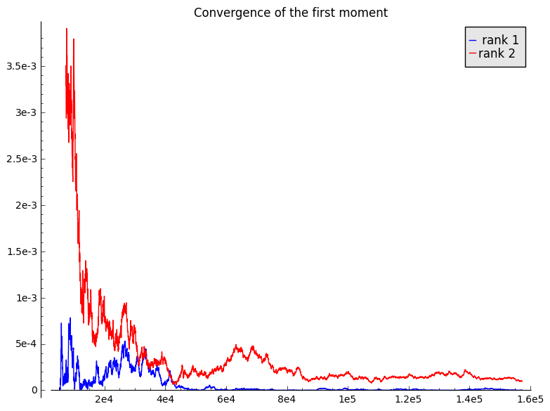
In Figure 1 we plot the function δ​(a1,x)2\delta(a_{1},x)^{2} for two elliptic curves AA and A′A^{\prime} of similar conductor and ranks 11 and 22. We indeed observe a better convergence of the curve of rank 11.

Refer to caption
Figure 1. Plot of δ​(a1,x)2\delta(a_{1},x)^{2} for the non-CM elliptic curves with LMFDB label 390.a1 (of rank 1) and 389.a1 (of rank 2).

6.1.2. Example 2: The Frobenius–Schur index also matters (g=1g=1).

Let AA, A′A^{\prime}, and φ0\varphi_{0} be as in §6.1.1, but suppose that now rA=1r_{A}=1 and rA′=0r_{A^{\prime}}=0. Now we have

I1​(φ)=(2⋅1−1)2=1,I1​(φ′)=(2⋅0−1)2=1.I_{1}(\varphi)=(2\cdot 1-1)^{2}=1\,,\qquad I_{1}(\varphi^{\prime})=(2\cdot 0-1)^{2}=1\,.
Refer to caption
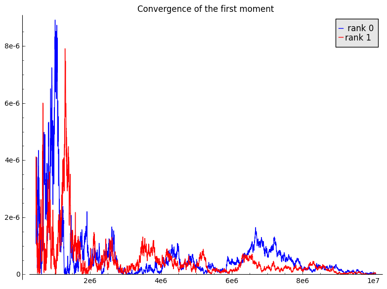
Figure 2. Plot of δ​(a1,x)2\delta(a_{1},x)^{2} for the non-CM elliptic curves with LMFDB label 37.b2 (of rank 0) and 37.a1 (of rank 1).

In Figure 2 we plot δ​(a1,x)2\delta(a_{1},x)^{2} for two non-CM elliptic curves of the same conductor and ranks 00 and 11. In this case we observe a similar convergence rate.

6.1.3. Example 3: The Sato–Tate group matters (g=1g=1).

Let AA (resp. A′A^{\prime}) be an elliptic curve defined over ℚ\mathbb{Q} without (resp. with) complex multiplication, and let φ0=a13\varphi_{0}=a_{1}^{3} be the cube of the trace character of USp⁡(2)\mathrm{USp}(2). We have G=USp⁡(2)G=\mathrm{USp}(2) and G′=U⁡(1)⋊ℤ/2​ℤG^{\prime}=\mathrm{U}(1)\rtimes\mathbb{Z}/2\mathbb{Z}.

Proposition 6.4.

If φ0\varphi_{0}, AA and A′A^{\prime} are as above, then

I1​(φ)=(4​rA+2​rSym3⁡(A)−3)2,I1​(φ′)=(4​rA′+2​rSym3⁡(A′)−4)2.I_{1}(\varphi)=(4r_{A}+2r_{\operatorname{Sym}^{3}(A)}-3)^{2}\,,\qquad I_{1}(\varphi^{\prime})=(4r_{A^{\prime}}+2r_{\operatorname{Sym}^{3}(A^{\prime})}-4)^{2}\,.
Proof.

From [Ser77, §8.2], one easily finds that the irreducible characters of G′G^{\prime} are

ϱm:=Tr⁡(IndU⁡(1)G′⁡(νm))\varrho_{m}:=\operatorname{Tr}(\operatorname{Ind}_{\mathrm{U}(1)}^{G^{\prime}}(\nu_{m}))

for m≥0m\geq 0, where νm\nu_{m} is as in (5.6). Let σ\sigma denote the nontrivial element of ℤ/2​ℤ\mathbb{Z}/2\mathbb{Z}. For (Au,s)∈U⁡(1)⋊ℤ/2​ℤ(A_{u},s)\in\mathrm{U}(1)\rtimes\mathbb{Z}/2\mathbb{Z}, one has

ϱm​(Au,s)={um+u−mif s is trivial,0if s=σ.\varrho_{m}(A_{u},s)=\begin{cases}u^{m}+u^{-m}&\text{if $s$ is trivial,}\\ 0&\text{if $s=\sigma$.}\end{cases}

It follows that φ′=3​ϱ1+ϱ3\varphi^{\prime}=3\varrho_{1}+\varrho_{3} and then, using Lemma 6.1, that

I1​(φ′)=(2​(rSym3⁡(A′)−rA′)−1+3​(2⋅rA′−1))2=(4​rA′+2​rSym3⁡(A′)−4)2I_{1}(\varphi^{\prime})=(2(r_{\operatorname{Sym}^{3}(A^{\prime})}-r_{A^{\prime}})-1+3(2\cdot r_{A^{\prime}}-1))^{2}=(4r_{A^{\prime}}+2r_{\operatorname{Sym}^{3}(A^{\prime})}-4)^{2}

Provided that φ=2​χ1+χ3\varphi=2\chi_{1}+\chi_{3}, where χn\chi_{n} is as in (5.4), we obtain that

I1​(φ)=((2⋅rχ3−1)+2​(2⋅rχ1−1))2=(4​rA+2​rSym3⁡(A)−3)2,I_{1}(\varphi)=\big((2\cdot r_{\chi_{3}}-1)+2(2\cdot r_{\chi_{1}}-1)\big)^{2}=(4r_{A}+2r_{\operatorname{Sym}^{3}(A)}-3)^{2}\,,

and the proposition follows. ∎

One can take now AA and A′A^{\prime} with similar conductors and such that rSym3⁡(A)=rSym3⁡(A′)r_{\operatorname{Sym}^{3}(A)}=r_{\operatorname{Sym}^{3}(A^{\prime})} and rA=rA′r_{A}=r_{A^{\prime}}. If we take these analytic ranks to be respectively 11 and 00, we find

I1​(φ)=1,I1​(φ′)=4.I_{1}(\varphi)=1\,,\qquad I_{1}(\varphi^{\prime})=4\,.

In Figure 3 we plot δ​(a13,x)2\delta(a_{1}^{3},x)^{2} for two curves AA, A′A^{\prime} with the above invariants. We observe that for large values of xx, even though the two plots cross many times, the one corresponding to the CM curve seems to have a larger asymptotic L2L^{2}-norm. In fact, we computed that

I⁡(φ,232)≃4.08,andI⁡(φ′,232)≃7.67.\displaystyle I(\varphi,2^{32})\simeq 4.08,\ \ \text{and}\ \ I(\varphi^{\prime},2^{32})\simeq 7.67.
Refer to caption
Figure 3. Plot of δ​(a13,x)2\delta(a_{1}^{3},x)^{2} for the rank 00 curves 40.a1 (non-CM) and 49.a1 (CM).
Remark 6.5.

Note that, in the situation considered, if we had taken φ0=a1\varphi_{0}=a_{1}, no significant difference would have been observed between the convergence of δ⁡(φ,x)\delta(\varphi,x) and δ⁡(φ′,x)\delta(\varphi^{\prime},x). Indeed, in this case, one finds I1​(φ)=(2⋅rA−1)2=(2⋅rA′−1)2=I1​(φ′)I_{1}(\varphi)=(2\cdot r_{A}-1)^{2}=(2\cdot r_{A^{\prime}}-1)^{2}=I_{1}(\varphi^{\prime}) (compare with §6.1.4).

6.1.4. Example 3’: The Sato–Tate group matters (g=1g=1).

We will now consider an example over a finite extension of ℚ\mathbb{Q}. Let KK be a quadratic imaginary field, AA be an elliptic curve defined over KK without CM, and A′A^{\prime} an elliptic curve defined over KK with CM precisely by KK. As in the previous example, let φ0=a13\varphi_{0}=a_{1}^{3}. Note that φ′\varphi^{\prime} is a selfdual character of U⁡(1)\mathrm{U}(1), even if its irreducible constituents are not.

Proposition 6.6.

If φ0\varphi_{0}, AA and A′A^{\prime} are as above, then

I1​(φ)=(4​rA+2​rSym3⁡(A)−3)2,I1​(φ′)=(4​rA′+2​rSym3⁡(A′))2.I_{1}(\varphi)=(4r_{A}+2r_{\operatorname{Sym}^{3}(A)}-3)^{2}\,,\qquad I_{1}(\varphi^{\prime})=(4r_{A^{\prime}}+2r_{\operatorname{Sym}^{3}(A^{\prime})})^{2}\,.
Proof.

Note that φ′=ν−3+3​ν−1+3​ν1+ν3\varphi^{\prime}=\nu_{-3}+3\nu_{-1}+3\nu_{1}+\nu_{3}, where νm\nu_{m} is as in (5.6). Using Lemma 6.1, one finds that

I1​(φ′)=((2⋅rν−3−0)+3​(2⋅rν−1−0)+3​(2⋅rν1−0)+(2⋅rν3−0))2=(4​rA′+2​rSym3⁡(A′))2.I_{1}(\varphi^{\prime})=\big((2\cdot r_{\nu_{-3}}-0)+3(2\cdot r_{\nu_{-1}}-0)+3(2\cdot r_{\nu_{1}}-0)+(2\cdot r_{\nu_{3}}-0)\big)^{2}=(4r_{A^{\prime}}+2r_{\operatorname{Sym}^{3}(A^{\prime})})^{2}\,.

The computation of I1​(φ)I_{1}(\varphi) is exactly as in Proposition 6.4. ∎

One can take now AA and A′A^{\prime} with similar conductors and such that rSym3⁡(A)=rSym3⁡(A′)r_{\operatorname{Sym}^{3}(A)}=r_{\operatorname{Sym}^{3}(A^{\prime})} and rA=rA′r_{A}=r_{A^{\prime}}. By Remark 6.3, we are forced to take AA and A′A^{\prime} to be the base change of elliptic curves A0A_{0} and A0′A_{0}^{\prime} defined over ℚ\mathbb{Q}. Then the following lemma implies that these two analytic ranks must be even and satisfy rSym3⁡(A′)≥rA′r_{\operatorname{Sym}^{3}(A^{\prime})}\geq r_{A^{\prime}}.

Lemma 6.7.

Let EE be an elliptic curve over ℚ\mathbb{Q} and E~\tilde{E} the quadratic twist of EE by the quadratic extension K/ℚK/\mathbb{Q}. Then

rEK=rE+rE~,rSym3⁡(EK)=rSym3⁡(E)+rSym3⁡(E~).r_{E_{K}}=r_{E}+r_{\tilde{E}}\,,\qquad r_{\operatorname{Sym}^{3}(E_{K})}=r_{\operatorname{Sym}^{3}(E)}+r_{\operatorname{Sym}^{3}(\tilde{E})}\,.

Moreover, if KK is imaginary and EE has CM by KK, then

rEK=2​rE,rSym3⁡(EK)=2​rSym3⁡(E),rSym3⁡(EK)≥rEK.r_{E_{K}}=2r_{E}\,,\qquad r_{\operatorname{Sym}^{3}(E_{K})}=2r_{\operatorname{Sym}^{3}(E)},\qquad r_{\operatorname{Sym}^{3}(E_{K})}\geq r_{E_{K}}\,.
Proof.

Let ε\varepsilon denote the quadratic character of K/ℚK/\mathbb{Q}. We have isomorphisms of ℚℓ​[Gℚ]\mathbb{Q}_{\ell}[G_{\mathbb{Q}}]-modules

IndGℚGK​Sym3⁡(Vℓ​(EK))≃Sym3⁡(Vℓ​(E))⊕Sym3⁡(Vℓ​(E))⊗ε≃Sym3⁡(Vℓ​(E))⊕Sym3⁡(Vℓ​(E~)),\operatorname{Ind}_{G_{\mathbb{Q}}}^{G_{K}}\operatorname{Sym}^{3}(V_{\ell}(E_{K}))\simeq\operatorname{Sym}^{3}(V_{\ell}(E))\oplus\operatorname{Sym}^{3}(V_{\ell}(E))\otimes\varepsilon\simeq\operatorname{Sym}^{3}(V_{\ell}(E))\oplus\operatorname{Sym}^{3}(V_{\ell}(\tilde{E}))\,,

and the first part of the lemma follows from the Artin Formalism of LL-functions. For the second part, one first needs to note that, under the additional hypothesis, one has

Vℓ​(E)≃Vℓ​(E)⊗ε≃Vℓ​(E~).V_{\ell}(E)\simeq V_{\ell}(E)\otimes\varepsilon\simeq V_{\ell}(\tilde{E})\,.

This follows from the fact that Tr⁡(Vℓ​(E))​(σ)=0\operatorname{Tr}(V_{\ell}(E))(\sigma)=0, whenever ε⁡(σ)≠1\varepsilon(\sigma)\not=1 for σ∈Gℚ\sigma\in G_{\mathbb{Q}}. One then concludes by noting that there is a Hecke character Φ\Phi such that

Symm⁡Vℓ​(EK)≃⨁j=0mΦm−2​j​(j),\operatorname{Sym}^{m}V_{\ell}(E_{K})\simeq\bigoplus_{j=0}^{m}\Phi^{m-2j}(j)\,,

where Φm−2​j​(j)\Phi^{m-2j}(j) denotes the jj-th Tate twist of Φm−2​j\Phi^{m-2j}. ∎

If we take for example rSym3⁡(A)=rSym3⁡(A′)=4r_{\operatorname{Sym}^{3}(A)}=r_{\operatorname{Sym}^{3}(A^{\prime})}=4 and rA=rA′=2r_{A}=r_{A^{\prime}}=2, we obtain

I1​(φ)=144,I2​(φ′)=256.I_{1}(\varphi)=144\,,\qquad I_{2}(\varphi^{\prime})=256\,.

In order to find examples of this type we have used [MW06, Table 7] for the non-CM curves, and Watkins’s Sympow package to find the CM curves with appropriate order of vanishing of the third symmetric power.

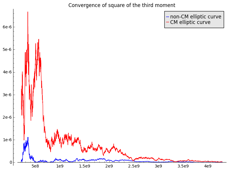
In Figure 3’ we plot δ​(a13,x)2\delta(a_{1}^{3},x)^{2} for two elliptic curves A/KA/K and A′/KA^{\prime}/K, where K=ℚ⁡(−3)K=\mathbb{Q}(\sqrt{-3}). The curve AA is the base change to KK of the curve with LMFDB label 97448.a2; its conductor is the ideal of KK generated by 9744897448, it does not have CM and its ranks are rA=2r_{A}=2 and rSym3⁡(A)=4r_{\operatorname{Sym}^{3}(A)}=4. The curve A′A^{\prime} is the base change to KK of the CM curve with LMFDB label 248004.g1; its conductor is the ideal of KK generated by 8266882668, it has CM by KK, and its ranks are rA′=2r_{A^{\prime}}=2 and rSym3⁡(A′)=4r_{\operatorname{Sym}^{3}(A^{\prime})}=4. We observe a better convergence for the non-CM curve.
Refer to caption
Figure 3’. Plot of δ​(a13,x)2\delta(a_{1}^{3},x)^{2} for two elliptic curves over ℚ⁡(−3)\mathbb{Q}(\sqrt{-3}) of rank 22 and rank of the symmetric cube 44, without CM and the other with CM by KK.
Remark 6.8.

In order to plot δ​(a13,x)2\delta(a_{1}^{3},x)^{2} one needs to recover the polynomials L𝔭​(A,T)L_{\mathfrak{p}}(A,T) from the polynomials Lp​(A0,T)L_{p}(A_{0},T) computed by Smalljac. This is straightforward. Let 𝔭{\mathfrak{p}} be an unramified prime of KK lying over pp. If 𝔭{\mathfrak{p}} is split over ℚ\mathbb{Q}, then Smalljac directly returns L𝔭​(A,T)=Lp​(A0,T)L_{\mathfrak{p}}(A,T)=L_{p}(A_{0},T). If 𝔭{\mathfrak{p}} is inert over ℚ\mathbb{Q}, then

L𝔭​(A,T)=(1−αp2)​(1−α¯p2)=1−(ap2−2)​T+T2,L_{\mathfrak{p}}(A,T)=(1-\alpha_{p}^{2})(1-\bar{\alpha}_{p}^{2})=1-(a_{p}^{2}-2)T+T^{2}\,,

where

Lp​(A0,T)=(1−αp)​(1−α¯p)=1−ap​T+T2.L_{p}(A_{0},T)=(1-\alpha_{p})(1-\bar{\alpha}_{p})=1-a_{p}T+T^{2}\,.
Remark 6.9.

For this example we could have taken φ0=a1\varphi_{0}=a_{1}. Similar computations show that then I1​(φ)=4​rA2I_{1}(\varphi)=4r_{A}^{2} and I1​(φ′)=(2​rA−1)2I_{1}(\varphi^{\prime})=(2r_{A}-1)^{2}.

6.1.5. Example 4: The rank matters (g=2g=2).

Let AA, A′A^{\prime}, A′′A^{\prime\prime}, and A′′′A^{\prime\prime\prime} be abelian surfaces of similar conductor, with Sato–Tate group USp⁡(4)\mathrm{USp}(4), and respective ranks 00, 11, 22, and 33. Letting φ0=a1\varphi_{0}=a_{1} and φ\varphi, φ′′\varphi^{\prime\prime},… have the obvious meaning, we have that

I1​(φ)=1,I1​(φ′)=1,I1​(φ′′)=9,I1​(φ′′′)=25.I_{1}(\varphi)=1\,,\qquad I_{1}(\varphi^{\prime})=1\,,\qquad I_{1}(\varphi^{\prime\prime})=9\,,\qquad I_{1}(\varphi^{\prime\prime\prime})=25\,.
Refer to caption
Figure 4. Plot of δ​(a1,x)2\delta(a_{1},x)^{2} for the (Jacobians of the) genus two curves with LMFDB labels 62127.a.62127.1 (of rank 0), 61929.a.433503.1 (rank 1), 62090.a.62090.1 (rank 2), and 62411.b.62411.1 (rank 3). They all have Sato–Tate group USp⁡(4)\mathrm{USp}(4), and the number in the label indicates the conductor of the curve.

In Figure 4 we plot the function δ​(a1,x)2\delta(a_{1},x)^{2} for four abelian surfaces of similar conductors and ranks 00, 11, 22, and 33.

6.1.6. Example 5: The Sato–Tate group matters (g=2g=2).

Let AA and A′A^{\prime} be abelian surfaces defined over ℚ\mathbb{Q} of similar conductor, with analytic rank rA=rA′=2r_{A}=r_{A^{\prime}}=2, but with Sato–Tate groups G=USp⁡(4)G=\mathrm{USp}(4) and G′=USp⁡(2)×USp⁡(2)G^{\prime}=\mathrm{USp}(2)\times\mathrm{USp}(2) (the group denoted by G3,3G_{3,3} in [FKRS12]). More specifically, suppose that A′A^{\prime} decomposes over ℚ\mathbb{Q} as the product of two nonisogenous elliptic curves of rank 11. Taking φ0=a1\varphi_{0}=a_{1}, we obtain

I1​(φ)=(2⋅2−1)2=9,I1​(φ′)=(2⋅1−1+2⋅1−1)2=4.I_{1}(\varphi)=(2\cdot 2-1)^{2}=9\,,\qquad I_{1}(\varphi^{\prime})=(2\cdot 1-1+2\cdot 1-1)^{2}=4\,.

An example of this phenomenon is shown in Figure 5.

Refer to caption
Figure 5. Plot of δ​(a1,x)2\delta(a_{1},x)^{2} for the genus two curves with LMFDB labels 16217.a.16217.1 (of rank 22 and Sato–Tate group USp⁡(4)\mathrm{USp}(4)) and 16245.c.925965.1 (of rank 22 and Sato–Tate group G3,3G_{3,3}).

6.1.7. Example 6: Non-optimality of the irreducible characters.

The goal of this example is to show that, although in §5 we demonstrated that the irreducible characters of USp⁡(2​g)\mathrm{USp}(2g) exhibit an extremely good convergence in the generic cases (and, in fact, almost optimal), one can find particular examples for which their convergence is beaten by some other family of characters, which are still a basis of the central functions. For example, let AA be an elliptic curve without CM such that rA=2r_{A}=2 and rSym3⁡(A)=0r_{\operatorname{Sym}^{3}(A)}=0. Let χn\chi_{n} be as in (5.4), and for n≥0n\geq 0 set

χn′:={χ1+χ3if n=1,χnotherwise.\chi_{n}^{\prime}:=\begin{cases}\chi_{1}+\chi_{3}&\text{if $n=1$,}\\ \chi_{n}&\text{otherwise.}\end{cases}

Clearly, {χn′}n≥0\{\chi_{n}^{\prime}\}_{n\geq 0} is also a basis of the central functions on GG, and I1​(χn)=I1​(χn′)I_{1}(\chi_{n})=I_{1}(\chi_{n}^{\prime}) for every n≠1n\not=1. However,

I1​(χ1)=(2⋅2−1)2>(2⋅2−1+2⋅0−1)2=I1​(χ1′).I_{1}(\chi_{1})=(2\cdot 2-1)^{2}>(2\cdot 2-1+2\cdot 0-1)^{2}=I_{1}(\chi_{1}^{\prime})\,.

In Figure 6 we plot δ​(χ1,x)2\delta(\chi_{1},x)^{2} and δ​(χ1+χ3,x)2\delta(\chi_{1}+\chi_{3},x)^{2} for the elliptic curve EE with LMFDB label 389.a1. It has rE=2r_{E}=2 and rSym3⁡E=0r_{\operatorname{Sym}^{3}E}=0. Even though χ1+χ3\chi_{1}+\chi_{3} is not always below χ1\chi_{1}, it does seem to close a smaller area.

Refer to caption
Figure 6. Plot of δ​(χ1,x)2\delta(\chi_{1},x)^{2} and δ​(χ1+χ3,x)2\delta(\chi_{1}+\chi_{3},x)^{2} for the elliptic curve EE with label 389.a1

6.2. Even weight

Let χ\chi be an irreducible character of GG and let wχw_{\chi} denote its weight. If wχw_{\chi} is odd, then (wχ+1)/2(w_{\chi}+1)/2 is an integer, and the Bloch–Kato conjecture predicts the order of the zero at (wχ+1)/2(w_{\chi}+1)/2 of the LL-function attached to χ​      ​ϱA\chi\begin{picture}(-3.0,-2.0)\put(0.0,1.0){\circle{2.0}}\end{picture}\varrho_{A}, which is precisely rχr_{\chi}.

If wχw_{\chi} is even, then (wχ+1)/2(w_{\chi}+1)/2 is no longer an integer and the Bloch–Kato conjecture makes no prediction for the order of vanishing of the LL-function attached to χ​      ​ϱA\chi\begin{picture}(-3.0,-2.0)\put(0.0,1.0){\circle{2.0}}\end{picture}\varrho_{A} at this point. The general philosophy is that rχr_{\chi} should be 00 unless there is a specific reason for the contrary to happen, and one thus expects rχ=0r_{\chi}=0 for χ\chi of even weight.

If χm,n\chi_{m,n} is as in (5.7), then (5.8) implies that χm,n\chi_{m,n} has even weight if and only if m+nm+n is even. One thus expects rχm,n=0r_{\chi_{m,n}}=0 whenever m+nm+n is even. Using [Wey97, §9, Chap. VII] again, one easily finds that

a2−1=χ1,1,a12−1=χ1,1+χ2,0,s2+1=−χ1,1+χ2,0.a_{2}-1=\chi_{1,1}\,,\qquad a_{1}^{2}-1=\chi_{1,1}+\chi_{2,0}\,,\qquad s_{2}+1=-\chi_{1,1}+\chi_{2,0}\,.

Let now AA be an abelian surface with Sato–Tate group USp⁡(4)\mathrm{USp}(4). By Lemma 6.1, we have

I1​(a2−1)=(2⋅0+1)2=1,I1​(a12−1)=(2⋅0+1+2⋅0+1)2=4I1​(s2+1)=(−(2⋅0+1)+(2⋅0+1))2=0.I_{1}(a_{2}-1)=(2\cdot 0+1)^{2}=1\,,\quad I_{1}(a_{1}^{2}-1)=(2\cdot 0+1+2\cdot 0+1)^{2}=4\quad I_{1}(s_{2}+1)=(-(2\cdot 0+1)+(2\cdot 0+1))^{2}=0\,.
Refer to caption
Figure 7. Plot of δ​(a12−1,x)2\delta(a_{1}^{2}-1,x)^{2}, δ​(a2−1,x)2\delta(a_{2}-1,x)^{2}, and δ​(s2+1,x)2\delta(s_{2}+1,x)^{2} for the genus two curve 277.a.277.1

In Figure 7 we plot δ​(a12−1,x)2\delta(a_{1}^{2}-1,x)^{2}, δ​(a2−1,x)2\delta(a_{2}-1,x)^{2}, and δ​(s2+1,x)2\delta(s_{2}+1,x)^{2}. Observe that, even though I1​(a2−1)>I1​(s2+1)I_{1}(a_{2}-1)>I_{1}(s_{2}+1), it is not clear from the figure whether the convergence for s2+1s_{2}+1 is better than the convergence for a2−1a_{2}-1. This seems to be explained by the fact that the difference I1​(a2−1)−I1​(s2+1)I_{1}(a_{2}-1)-I_{1}(s_{2}+1) is small together with the fact that I2​(a2−1)≤I2​(s2+1)I_{2}(a_{2}-1)\leq I_{2}(s_{2}+1). Nonetheless, in the range of primes that we have considered, one clearly sees a slower rate of convergence for a12−1a_{1}^{2}-1 than for a2−1a_{2}-1 and s2+1s_{2}+1.

7. Chebyshev bias for abelian varieties

As we noted in §1, the circle of ideas we used to study the convergence rate towards the Sato–Tate measure was introduced by Sarnak in his letter to Mazur [Sar07], in order to explain the bias that the Frobenius traces of elliptic curves have towards being positive or negative, and how the rank determines the sign of the bias.

Not surprisingly, then, one can also use this approach to study this phenomenon for general abelian varieties. Indeed, resuming the notations of §​1\lx@sectionsign\ref{section: intro}, for a selfdual virtual character φ=∑χ≠1cχ​χ\varphi=\sum_{\chi\not=1}c_{\chi}\chi of GG, recall the function

(7.1) ψ⁡(φ,x)=log⁡(x)x​∑|𝔭|≤xφ⁡(y𝔭).\displaystyle\psi(\varphi,x)=\frac{\log(x)}{\sqrt{x}}\sum_{|{\mathfrak{p}}|\leq x}\varphi(y_{\mathfrak{p}}).

Recall that by (3.10) we have

limX→∞1log⁡(X)∫2Xψ(φ,x)xd​x=−∑χcχ(2rχ+uχ).\displaystyle\lim_{X\rightarrow\infty}\frac{1}{\log(X)}\int_{2}^{X}{\psi(\varphi,x)}\frac{x}{dx}=-\sum_{\chi}c_{\chi}(2r_{\chi}+u_{\chi})\,.

In the case of elliptic curves, the bias of a1a_{1} towards being positive or negative only depends on the rank. In higher dimensions, the above formula shows that it also depends on the Sato–Tate group. For example, suppose that AA is an abelian surface of rank rA=1r_{A}=1 and Sato–Tate group USp⁡(4)\mathrm{USp}(4). Then the right hand side of (3.10) equals −(2​rA−1)=−1-(2r_{A}-1)=-1, and a1a_{1} has a bias towards being negative. Suppose now that A′A^{\prime} is an abelian surface of rank rA′=1r_{A^{\prime}}=1 and Sato–Tate group G3,3G_{3,3}. Suppose that A′A^{\prime} is isogenous to the product of two elliptic curves, say EE and E′E^{\prime}, of ranks rE=1r_{E}=1 and rE′=0r_{E^{\prime}}=0. Then the right hand side of (3.10) equals −(2​rE−1)−(2​rE′−1)=0-(2r_{E}-1)-(2r_{E^{\prime}}-1)=0, and the a1a_{1}’s do not have bias towards being positive nor negative. In Figure 8 we plot the function δ⁡(a1,x)\delta(a_{1},x) for two abelian surfaces AA and A′A^{\prime} having these ranks and Sato–Tate groups. The prediction on the bias of the sign of a1a_{1} can be clearly observed.

Refer to caption
Figure 8. Plot of δ⁡(a1,x)\delta(a_{1},x) for the genus two curve 2165.a.2165.1 (rank 11 and Sato–Tate group USp⁡(4)\mathrm{USp}(4)) and for 2156.b.34496.1 (rank 11 and Sato–Tate group G3,3G_{3,3}).

References

  • [ANS14] Amir Akbary, Nathan Ng, and Majid Shahabi, Limiting distributions of the classical error terms of prime number theory, Q. J. Math. 65 (2014), no. 3, 743–780. MR 3261965
  • [BK16a] Grzegorz Banaszak and Kiran S. Kedlaya, Motivic Serre group, algebraic Sato-Tate group and Sato-Tate conjecture, Frobenius distributions: Lang-Trotter and Sato-Tate conjectures, Contemp. Math., vol. 663, Amer. Math. Soc., Providence, RI, 2016, pp. 11–44. MR 3502937
  • [BK16b] Alina Bucur and Kiran S. Kedlaya, An application of the effective Sato-Tate conjecture, Frobenius distributions: Lang-Trotter and Sato-Tate conjectures, Contemp. Math., vol. 663, Amer. Math. Soc., Providence, RI, 2016, pp. 45–56. MR 3502938
  • [Cog03] J. W. Cogdell, Langlands conjectures for GLn{\rm GL}_{n}, An introduction to the Langlands program (Jerusalem, 2001), Birkhäuser Boston, Boston, MA, 2003, pp. 229–249. MR 1990381
  • [FH91] William Fulton and Joe Harris, Representation theory, Graduate Texts in Mathematics, vol. 129, Springer-Verlag, New York, 1991, A first course, Readings in Mathematics. MR 1153249
  • [Fio14] Daniel Fiorilli, Elliptic curves of unbounded rank and Chebyshev’s bias, Int. Math. Res. Not. IMRN (2014), no. 18, 4997–5024. MR 3264673
  • [FKRS12] Francesc Fité, Kiran S. Kedlaya, Víctor Rotger, and Andrew V. Sutherland, Sato-Tate distributions and Galois endomorphism modules in genus 2, Compos. Math. 148 (2012), no. 5, 1390–1442. MR 2982436
  • [Gup87] R. K. Gupta, Characters and the qq-analog of weight multiplicity, J. London Math. Soc. (2) 36 (1987), no. 1, 68–76. MR 897675
  • [IK04] Henryk Iwaniec and Emmanuel Kowalski, Analytic number theory, American Mathematical Society Colloquium Publications, vol. 53, American Mathematical Society, Providence, RI, 2004. MR 2061214
  • [KS08] Kiran S. Kedlaya and Andrew V. Sutherland, Computing LL-series of hyperelliptic curves, Algorithmic number theory, Lecture Notes in Comput. Sci., vol. 5011, Springer, Berlin, 2008, pp. 312–326. MR 2467855
  • [KS09] by same author, Hyperelliptic curves, LL-polynomials, and random matrices, Arithmetic, geometry, cryptography and coding theory, Contemp. Math., vol. 487, Amer. Math. Soc., Providence, RI, 2009, pp. 119–162. MR 2555991
  • [Maz08] Barry Mazur, Finding meaning in error terms, Bull. Amer. Math. Soc. (N.S.) 45 (2008), no. 2, 185–228. MR 2383303
  • [MS13] Barry Mazur and William Stein, How Explicit is the Explicit Formula?, Available at http://www.math.harvard.edu/~mazur/papers/How.Explicit.pdf.
  • [Mur85] V. Kumar Murty, Explicit formulae and the Lang-Trotter conjecture, Rocky Mountain J. Math. 15 (1985), no. 2, 535–551, Number theory (Winnipeg, Man., 1983). MR 823264
  • [MW06] Phil Martin and Mark Watkins, Symmetric powers of elliptic curve LL-functions, Algorithmic number theory, Lecture Notes in Comput. Sci., vol. 4076, Springer, Berlin, 2006, pp. 377–392. MR 2282937
  • [RS94] Michael Rubinstein and Peter Sarnak, Chebyshev’s bias, Experiment. Math. 3 (1994), no. 3, 173–197. MR 1329368
  • [Sar07] Peter Sarnak, Letter to Barry Mazur on “Chebyshev’s bias” for τ⁡(p)\tau(p).
  • [Ser68] Jean-Pierre Serre, Abelian ll-adic representations and elliptic curves, McGill University lecture notes written with the collaboration of Willem Kuyk and John Labute, W. A. Benjamin, Inc., New York-Amsterdam, 1968. MR 0263823
  • [Ser70] by same author, Facteurs locaux des fonctions zêta des variétés algébriques (définitions et conjectures), Séminaire Delange-Pisot-Poitou. Théorie des nombres 11.2, 1969-1970, pp. 1–15.
  • [Ser77] by same author, Linear representations of finite groups, Springer-Verlag, New York-Heidelberg, 1977, Translated from the second French edition by Leonard L. Scott, Graduate Texts in Mathematics, Vol. 42. MR 0450380
  • [Ser94] by same author, Propriétés conjecturales des groupes de Galois motiviques et des représentations ll-adiques, Motives (Seattle, WA, 1991), Proc. Sympos. Pure Math., vol. 55, Amer. Math. Soc., Providence, RI, 1994, pp. 377–400. MR 1265537
  • [Shi16] Yih-Dar Shieh, Character theory approach to Sato-Tate groups, LMS J. Comput. Math. 19 (2016), no. suppl. A, 301–314. MR 3540962
  • [Wey97] Hermann Weyl, The classical groups, Princeton Landmarks in Mathematics, Princeton University Press, Princeton, NJ, 1997, Their invariants and representations, Fifteenth printing, Princeton Paperbacks. MR 1488158