A Normalization Model for Analyzing Multi-Tier Millimeter Wave Cellular NetworksThanks: The corresponding author is Lijun Wang (e-mail: wanglijun@whu.edu.cn).

Given the dearth of spectrum in sub-3GHz bands, use of higher frequency bands is indispensable to meet the projected data demands of 2020 [1]. Faced with this challenge, cellular systems based on the millimeter wave (mmWave) bands has been attracted lots of interest, between 30 and 300 GHz, where the available bandwidths are much wider than today’s cellular networks [2, 3]. Recent field measurements also reveal the prospect of mmWave signals for the access link between the user equipment (UE) and base station (BS) in cellular systems [4].

Evaluating the system performance of mmWave cellular networks is a crucial task in order to understand the network behavior. Recently, several studies analyze the coverage performance and capacity in mmWave cellular networks using results from stochastic geometry [5, 6]. In [7], a tractable model is proposed for user’s rate distribution in noise-limited mmWave cellular networks, and a general framework has been proposed to evaluate coverage performance of the mmWave networks in [8]. However, one must remember that the mmWave cellular communication is easily affected by propagation environmental factors such as atmospheric conditions and physical obstacles, so the analysis of system-level performance evaluation of mmWave cellular network is usually single-tier network. [9] shows that cellular networks are becoming less regular as a variety of demand-based low power nodes are being deployed, and small cell networks were studied in recently literature [10, 11, 12]. Therefore, the networks could be regarded as the multi-tier cellular networks instead of the simple single-tier network. Moreover, as one of the candidate technologies in 5G, mmWave will be widely applied to various BSs with different transmit powers, antenna gains, etc [3]. Therefore, the emergence of multi-tier mmWave cellular networks is inevitable.

Recently a few researchers have presented some initial analysis of multi-tier mmWave cellular networks with the aid of stochastic geometry [13]. However, the mathematical framework for multi-tier mmWave cellular networks is not clear, and currently available mathematical framework presented on [14, 15] for modeling micro wave cellular networks is not directly applicable to mmWave cellular networks. The main reasons are related to the need of incorporating realistic path-loss, blockage models and highly directional antenna gains. They are significantly different from micro wave communications. The investigations [3, 16] have demonstrated large bandwidth mmWave networks tend to be noise-limited in urban settings with blocking, in contrast to micro wave cellular networks, which are interference-limited. Therefore, a tractable model for characterizing the multi-tier mmWave cellular networks seems important to develop.

In this paper, we aim at proposing a normalization model which can simplify analysis of multi-tier mmWave cellular networks. To the best of our knowledge, the works converting multi-tier networks into single-tier network in mmWave communication systems have not yet been analyzed until now. Moreover, we derived the end-to-end signal-to-noise ratio (SNR) in general case with beamforming alignment errors in the communication, and discussed the SNR in perfect beamforming alignment case. The numerical results proved that the normalization model is an effective model for analysis of multi-tier mmWave cellular networks.

In this section, we introduce our system model for down-link multi-tier mmWave cellular networks composed of $K$ independent network tiers of BSs with different deployment densities, transmit powers, and antenna gains. It is assumed that the BSs belonging to $k$-th tier are distributed uniformly in $\mathbb{R}^{2}$ according to a bi-dimensional homogeneous Poisson point process (PPP) $\Phi_{k}$ of density $\lambda_{k}$ , and have transmit power $P_{k}$ and the same beam width of the main lobe $\omega\in\left(0,2\pi\right)$. Assuming that the multiple cells of different tiers are distributed in the same plane, then, the distribution of the BSs in multi-tier mmWave networks is defined as $\Phi=\cup_{k=1}^{K}\Phi_{k}$ with density $\lambda=\sum_{k=1}^{K}\lambda_{k}$. Without loss of generality, the typical UE is assumed to be located at the origin $\left(0,0\right)$ and the distance between an arbitrary BS and typical UE is $x$.

Different from the single-tier mmWave cellular network where all BSs have the same transmit power, beam width and the main lobe gain, in multi-tiers mmWave cellular networks, the BSs of different tiers have different parameters in power, beam width and follow different distributions geographically. The complexity of the scenario leads to many difficulties and enormous computing work in the performance analysis. In order to make the analysis clearer, we propose a normalization model in this paper, which converts a multi-tier mmWave cellular networks to a virtual single-tier cellular network by the method of scaling. Unlike our previous works [17], which proposed a transmission power normalization model for conventional multi-tier heterogeneous cellular networks, our model in this paper takes LOS/NLOS paths and directional beamforming into consideration, which are critical factors to mmWave networks. As a result, all BSs have the same normalized transmission power 1, and then, the virtual distance and link type which is either LOS or NLOS become two important factors that affect the UE’s received power.

In a $K$-Tier mmWave networks, the BSs in tier $k$, $k\in\left\{1,2,\cdots,K\right\}$, have transmit power $p_{k}$, beam width of the main lobe $\omega_{k}$ and follow homogeneous PPP $\Phi_{k}$ of density $\lambda_{k}$. Due to the characteristic of mmWave communication link, we assume each tier network is split into two parts. Let $\Phi_{k}^{L}$ be the point process of $k$-th tier LOS BSs, and $\Phi_{k}^{N}=\Phi_{k}\setminus\Phi_{k}^{L}$ be the point process of $k$-th tier NLOS BSs. The distribution of all BSs in whole networks can be described as $\Phi=\cup_{k=1}^{K}\Phi_{k}=\cup_{k=1}^{K}\left(\Phi_{k}^{L}+\Phi_{k}^{N}\right)$. Then, we will discuss separately the normalization model in two parts (scaled by LOS factors and scaled by NLOS factors).

The received signal power at the typical UE from the BS at $\mathbf{x}\in\Phi_{k}$ is given as

where 1 is the normalized transmit power and $L\left(\mathbf{x}\right)$ is the path loss function, and $j\in\left\{1,2,3,4\right\}$ indicates that the user is associated with LOS BS in different four cases. For example, $p_{k1}$ is the received signal power of typical UE in the case where the main lobe of UE and serving BS are aligned.

From (5), it is observed that the signal power received at the typical UE located at $\left(0,0\right)$ from the BS at $\mathbf{x}$ is equal to that received from the virtual BS with transmit power 1 and located at $\mathbf{x}_{L}=\left(p_{k}a_{j}\right)^{-\frac{1}{\alpha_{L}}}\cdot\mathbf{x}$. Based on this, the $k$-th tier homogeneous PPP $\Phi_{k}$ can be respectively scaled to $\Phi_{kj}^{{}^{\prime}}=\left(p_{k}a_{j}\right)^{-\frac{1}{\alpha_{L}}}\Phi_{k}$ of the scaled density $\lambda_{kj}^{{}^{\prime}}=\left(\frac{1}{\left(p_{k}a_{j}\right)^{-\frac{1}{\alpha_{L}}}}\right)^{2}\lambda_{k}=\left(p_{k}a_{j}\right)^{\frac{2}{\alpha_{L}}}\lambda_{k}$. Simultaneously, the radius $d$ of LOS circle will be scaled by different factors in each tier network, the LOS probability function by LOS scaling factors is given by

where $d_{kj}=d\cdot\left(p_{k}a_{j}\right)^{-\frac{1}{\alpha_{L}}}$, that is the scaled radius of LOS circle in $k$-th tier networks and in four beamforming alignment cases. For every $j\in\left\{1,2,3,4\right\}$, let $\mathcal{D}_{j}=\left\{d_{kj},k\in\left\{1,\ldots,K\right\}\right\}$ denote the set of scaled radius of $k$-th tier networks LOS circle, and suppose that the elements of $\mathcal{D}_{j}$ are indexed in an increasing order, that is $d_{\upsilon\left(1\right)j}\leq d_{\upsilon\left(2\right)j}\leq\cdots\leq d_{\upsilon\left(K\right)j}$ , and define $\gamma_{ij}=d_{\upsilon\left(i\right)j}$ as the scaled radius of LOS circle in the order list $\gamma_{j}=\left\{\gamma_{1j},\ldots,\gamma_{Kj}\right\}$. And the corresponding scaled density can be written as $\lambda_{\upsilon\left(i\right)j}^{{}^{\prime}}=\left(p_{\upsilon\left(i\right)}a_{\upsilon\left(i\right)j}\right)^{\frac{2}{\alpha_{L}}}\lambda_{\upsilon\left(i\right)}$. The densities of the $K$-tier networks scaled by the LOS factors in LOS circle can be given as

where $\mathbb{I}\left(\cdot\right)$ is the indicator function, $\mathcal{C}=\left\{0,1,\ldots,i-1\right\}$ denotes the subset of the set $\mathrm{\mathcal{K}=}\left\{0,1,\ldots,K\right\}$, its supplementary set is $\mathcal{C^{\mathcal{C}}}=\left\{i,\ldots,K\right\}$, and $\gamma_{0j}=0$. For ease of analysis, the second term of (III) is the scaled density of LOS BS outside LOS circle. It is worth noting that the densities in (III) are scaled from the densities BSs in all tiers within the circle of radius $d$ including LOS BSs and NLOS BSs, and we can get the LOS BSs densities in four beamforming alignment cases which are $C\cdot\lambda_{j}^{L}$ respectively. The normalization model scaled by LOS scaling factors is equivalent to converting $K$-tier mmWave networks to the virtual single-tier mmWave network, in which there are the same four beamforming alignment cases and the scaled densities respectively follow piecewise constant functions which have $K$ demarcation points in every case.

To explain this, consider a 2-tier mmWave network in LOS circle shown in Fig. 1. According to (3), the BSs located outside the circle of radius $d$ are NLOS BSs. In Fig. 1, BS $i$ is located at $\mathbf{x}_{ki}$ in $k$-th tier including BSs at $\mathbf{x}_{1i}$ in tier 1, and BSs at $\mathbf{x}_{2i}$ in tier 2, with different transmit powers and four directivity gains. The typical UE receives the desired signal from the associated BS located at $\mathbf{x}_{ki}$. For ease of analysis, we scale each tier by using different factors such that virtual BSs at $\mathbf{x}_{L1i}^{{}^{\prime}}$, $\mathbf{x}_{L2i}^{{}^{\prime}}$ with the same normalized power 1 are obtained, at the same time, the radius $d$ of LOS circle is scaled to $d_{1j}$ and $d_{2j}$ by different scaling factors so that the scaled density (BSs located in circle of radius $d_{1j}$) is the sum of 2 tiers scaled density that is $\lambda_{1j}^{{}^{\prime}}+\lambda_{2j}^{{}^{\prime}}$ as well as the scaled density (BSs located at circular ring area between radius $d_{1j}$ and $d_{2j}$ ) is $\lambda_{2j}^{{}^{\prime}}$. Moreover, the probability of LOS BSs located outside circle of radius $d_{2j}$ is 0, the scaled densities of BSs in the LOS circle can be given as $\lambda_{j}^{L}=\left(\lambda_{1j}^{{}^{\prime}}+\lambda_{2j}^{{}^{\prime}}\right)\mathnormal{\mathbb{I}\left(0<x^{L}\leq d_{1j}\right)}$+$\lambda_{2j}^{{}^{\prime}}\mathbb{I}\left(d_{ij}<x^{L}\leq d_{2j}\right)+0\cdot\left(d_{2j}<x^{L}\right)$. It is worth emphasizing that the scaled densities respectively follow piecewise constant functions which have two demarcation points in four alignment cases and the probability of LOS BSs is $C$ in the circle of radius $d_{2j}$, and the scaled densities of LOS BSs are equal to $C\cdot\lambda_{j}^{L}$.

It is known that the typical user does not directly communicate with an NLOS BS, instead they communicate by radio wave’s reflection and scattering, etc, so that the directivity gains can be ignored. Assume the typical user be associated with NLOS BS, according to (5), there is only a case $a_{j}=1$ for all $j$ in $\left\{1,2,3,4\right\}$. And the signal power received at the typical UE from the BS at $\mathbf{x}$ is equal to that received from the virtual BS $\mathbf{x}_{N}=\left(p_{k}\right)^{-\frac{1}{\alpha_{N}}}\cdot\mathbf{x}$ with transmit power 1 and located at $\left(p_{k}\right)^{-\frac{1}{\alpha_{N}}}\cdot\mathbf{x}$. Similarly, the $k$-th tier PPP $\Phi_{k}$ is scaled to $\Phi_{k}^{{}^{\prime}}=\left(p_{k}\right)^{-\frac{1}{\alpha_{N}}}\Phi_{k}$ of the scaled density $\lambda_{k}^{{}^{\prime}}=\left(p_{k}\right)^{\frac{2}{\alpha_{N}}}\lambda_{k}$. The radius $d$ of LOS circle is scaled to $d_{k}^{{}^{\prime}}=d\cdot p_{k}^{-\frac{1}{\alpha_{N}}}$, and let $\mathcal{D}=\left\{d_{k},k\in\left\{1,\ldots,K\right\}\right\}$ denote the set of scaled radius of $k$-th tier network LOS circle, and suppose that the elements of $\mathcal{D}$ are indexed in an increasing order, such that $d_{\upsilon\left(1\right)}\leq d_{\upsilon\left(2\right)}\leq\cdots\leq d_{\upsilon\left(K\right)}$ , and define $\gamma_{i}=d_{\upsilon\left(i\right)}$ as the scaled radius of LOS circle in the order list $\gamma=\left\{\gamma_{1},\ldots,\gamma_{K}\right\}$ , and the scaled density of BSs in $\upsilon\left(i\right)$-th tier mmWave network is $\lambda_{\upsilon\left(i\right)}^{{}^{\prime}}=\left(p_{\upsilon\left(i\right)}\right)^{\frac{2}{\alpha_{N}}}\lambda_{\upsilon\left(i\right)}$. The density of the $K$-tier mmWave networks scaled by the NLOS scaling factors in the LOS circle of radius $d$ with the NLOS probability $\left(1-p_{los}\left(x\right)\right)$ can be given by

where $\gamma_{0}=0$, and the scaled density of BSs outside the LOS circle of radius $d$ with the NLOS probability 1 can be given by

where $\lambda_{\upsilon\left(0\right)}^{{}^{\prime}}=0$. From (III) and (III), we can get $\lambda_{1}^{N}+\lambda_{2}^{N}=\underset{\mathit{{\scriptstyle l\in\mathcal{K}}}}{\sum}\mathnormal{\lambda_{\upsilon\left(l\right)}^{{}^{\prime}}}$ that is scaled density of PPP $\Phi^{{}^{\prime}}=\cup_{k=1}^{K}\Phi_{k}^{{}^{\prime}}$ by the NLOS factors scaling. According to (III), the scaled density of NLOS BSs in circle of radius $\gamma_{K}$ can be expressed as $\left(1-C\right)\lambda_{1}^{N}$. Similarly, from (III), the scaled density of NLOS BSs outside the circle of radius $\gamma_{1}$ can be expressed as $1\cdot\lambda_{2}^{N}$.

In Section IV, a general and tractable model for computing coverage and rate of mmWave systems is provided, based on the assumptions of $K$-tier mmWave cellular networks and a simple but flexible statistical blockage model. With these assumptions, a virtual single-tier mmWave network is presented with the new density of BSs. In this section, assuming the typical UE is associated with the nearest BS in normalization model, so the typical UE can receive the maximum signal power from that BS in $K$-tier mmWave cellular networks. And then the expression of the coverage probability is provided for high-SNR in general case (with beamforming alignment errors) and the special case (with perfect beamforming alignment) based on the normalization model.

The coverage probability of $K$-tier mmWave cellular networks can be given as

where $\mathbf{\mathbb{P}_{los}}$ is the probability when the typical UE can be served by the nearest BS with LOS path, $\mathbf{\mathbb{P}_{nlos}}$ is the probability when the typical UE can be served by the nearest BS with NLOS path. Then, we will respectively discuss the coverage probabilities in two cases.

In this section, we explore the relationship between beam width and maximum coverage probability with beamforming alignment errors. And without loss of generality, we present some simulation results for illustrating the normalization model and characterizing the coverage performance of the 2-tier mmWave networks as well as the effect of different network parameters. In all figures, LOS and NLOS path loss exponents are $\alpha_{L}=2$ and $\alpha_{N}=4$, respectively.

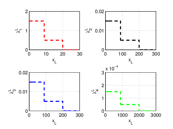
In order to characterize the model clearer, the scaled densities which are converted from 2-tier mmWave cellular networks to single-tier network are shown in Fig. 2. There are four scaled densities in different beamforming alignment state of 2. In Fig. 2, the 2nd graph and the 3rd graph is the same, because we assume the same beam width of the main lobe between user and BSs, the directivity gains in the cases $j=2$ and case $j=3$ are the same. The scaled densities follow piecewise constant functions. The piecewise points are affected by directivity gains and transmit powers, respectively, which provide convenience for performance analysis in multi-tier mmWave cellular networks. And the densities scaled by NLOS scaling factors are similar to that.

In Fig. 3, we compare coverage probability based on different $\left(C,d\right)$ pairs in perfect beamforming alignment and beamforming alignment errors cases. The empirical $\left(C,d\right)$ pair for Manhattan is $\left(0.117,200\right)$ [16]. In addition, two special cases with LOS $\left(C=1\right)$ and NLOS $\left(C=0\right)$ in the inner circle of radius $d=200$ are considered, and it can be interpreted to the upper limit and lower limit of coverage probability in beamforming alignment errors cases. From the Fig. 3, the coverage probability under the condition of perfect beamforming alignment is higher than that in beamforming alignment errors case at the same threshold. However, as the LOS probability $C$ decreases, the difference becomes smaller until it tends to zero.

In Fig. 4, the effect of beam widths on the coverage performance is analyzed in different SNR threshold. It is considered that the UE’s beam width is equal to the BS’s beam width and the side lobe strength $m_{q}=\epsilon$ is fixed in simulation. From Fig. 4, we can see that there exists a beam width to meet the highest coverage probability at the same threshold. And it can be interpreted that the smaller the beam width is, the greater the main lobe gain and the beamforming alignment errors are, so that there will be the beam width which makes the coverage probability maximum at the same threshold.

In this paper, a normalization model for simplifying analysis and computation of multi-tier mmWave cellular networks was introduced. Its novelty lies in converting the multi-tier mmWave cellular networks into a virtual single-tier mmWave network, where all BSs have the same normalized transmit power 1 and the scaled densities respectively follow corresponding piecewise constant functions. We have adopted the proposed approach to analyzing some coverage performance and the effect of beamforming alignment errors based on the noise-limited mmWave cellular systems in this paper. Numerical simulations have confirmed that the results met the analysis requirements. In future work, it would be interesting to analyze more system performances under the normalization model.

The authors would like to acknowledge the support of the International Science and Technology Cooperation Program of China (Grant Nos. 2015DFG12580 and 2014DFA11640), the National Natural Science Foundation of China (Grant Nos. 61471180, 61461136004, 61301147, 61471347, and 61210002), the Hubei Provincial Department of Education Scientific Research Project (Grant No. B2015188), the Shanghai Natural Science Foundation (Grant No. 16ZR1435100), the Fundamental Research Funds of Shandong University (Grant No. 2016JC010), a grant from Wenhua College (Grant No. 2013Y08), the National Research Foundation of Korea-Grant funded by the Korean Government (Ministry of Science, ICT and Future Planning)-NRF-2014K1A3A1A20034987), the EU FP7-PEOPLE-IRSES (Grant No. 610524), and the EU H2020 project (Grant No. 723227). This research is supported by the China International Joint Research Center of Green Communications and Networking (No. 2015B01008).

References

- [1] Cisco, “Cisco visual networking index: Global mobile data traffic forecast update, 2015-2020,” Whitepaper, [Online]. available at: http://goo.gl/SwuEIc, Feb 2016.
- [2] Z. Pi and F. Khan, “An introduction to millimeter-wave mobile broadband systems,” IEEE Communications Magazine, vol. 49, no. 6, pp. 101–107, June 2011.
- [3] S. Rangan, T. S. Rappaport, and E. Erkip, “Millimeter-wave cellular wireless networks: Potentials and challenges,” Proceedings of the IEEE, vol. 102, no. 3, pp. 366–385, March 2014.
- [4] T. S. Rappaport, F. Gutierrez, E. Ben-Dor, J. N. Murdock, Y. Qiao, and J. I. Tamir, “Broadband millimeter-wave propagation measurements and models using adaptive-beam antennas for outdoor urban cellular communications,” IEEE Transactions on Antennas and Propagation, vol. 61, no. 4, pp. 1850–1859, April 2013.
- [5] T. Bai, A. Alkhateeb, and R. W. Heath, “Coverage and capacity of millimeter-wave cellular networks,” IEEE Communications Magazine, vol. 52, no. 9, pp. 70–77, September 2014.
- [6] M. N. Kulkarni, S. Singh, and J. G. Andrews, “Coverage and rate trends in dense urban mmwave cellular networks,” in 2014 IEEE Global Communications Conference, Dec 2014, pp. 3809–3814.
- [7] S. Singh, M. N. Kulkarni, and J. G. Andrews, “A tractable model for rate in noise limited mmwave cellular networks,” in 2014 48th Asilomar Conference on Signals, Systems and Computers, Nov 2014, pp. 1911–1915.
- [8] T. Bai and R. W. Heath, “Coverage and rate analysis for millimeter-wave cellular networks,” IEEE Transactions on Wireless Communications, vol. 14, no. 2, pp. 1100–1114, Feb 2015.
- [9] A. Ghosh, N. Mangalvedhe, R. Ratasuk, B. Mondal, M. Cudak, E. Visotsky, T. A. Thomas, J. G. Andrews, P. Xia, H. S. Jo, H. S. Dhillon, and T. D. Novlan, “Heterogeneous cellular networks: From theory to practice,” IEEE Communications Magazine, vol. 50, no. 6, pp. 54–64, June 2012.
- [10] X. Ge, H. Cheng, M. Guizani, and T. Han, “5g wireless backhaul networks: challenges and research advances,” IEEE Network, vol. 28, no. 6, pp. 6–11, Nov 2014.
- [11] X. Ge, S. Tu, T. Han, Q. Li, and G. Mao, “Energy efficiency of small cell backhaul networks based on gauss-markov mobile models,” IET Networks, vol. 4, no. 2, pp. 158–167, 2015.
- [12] X. Ge, S. Tu, G. Mao, C. X. Wang, and T. Han, “5g ultra-dense cellular networks,” IEEE Wireless Communications, vol. 23, no. 1, pp. 72–79, February 2016.
- [13] M. D. Renzo, “Stochastic geometry modeling and analysis of multi-tier millimeter wave cellular networks,” IEEE Transactions on Wireless Communications, vol. 14, no. 9, pp. 5038–5057, Sept 2015.
- [14] H. S. Dhillon, R. K. Ganti, F. Baccelli, and J. G. Andrews, “Modeling and analysis of k-tier downlink heterogeneous cellular networks,” IEEE Journal on Selected Areas in Communications, vol. 30, no. 3, pp. 550–560, April 2012.
- [15] X. Ge, B. Yang, J. Ye, G. Mao, C. X. Wang, and T. Han, “Spatial spectrum and energy efficiency of random cellular networks,” IEEE Transactions on Communications, vol. 63, no. 3, pp. 1019–1030, March 2015.
- [16] S. Singh, M. N. Kulkarni, A. Ghosh, and J. G. Andrews, “Tractable model for rate in self-backhauled millimeter wave cellular networks,” IEEE Journal on Selected Areas in Communications, vol. 33, no. 10, pp. 2196–2211, Oct 2015.
- [17] T. Han, G. Mao, Q. Li, L. Wang, and J. Zhang, “Interference minimization in 5g heterogeneous networks,” Mobile Networks and Applications, vol. 20, no. 6, pp. 756–762, 2015.
- [18] J. Wildman, P. H. J. Nardelli, M. Latva-aho, and S. Weber, “On the joint impact of beamwidth and orientation error on throughput in directional wireless poisson networks,” IEEE Transactions on Wireless Communications, vol. 13, no. 12, pp. 7072–7085, Dec 2014.