跳到论文正文
W Papers独立论文阅读器 arXiv:1703.03101 论文正文 计算阅读时间 · 0%
引用这篇论文根据当前论文元数据生成,正式投稿前建议核对。


License: arXiv.org perpetual non-exclusive license
arXiv:1703.03101v1 [eess.SY] 09 Mar 2017

Robust MPC for tracking of nonholonomic robots with additive disturbancesfootnoteinfo

Zhongqi Sun Email: sunzhongqi12@gmail.com    Li Dai Email: daili1887@gmail.com    Kun Liu Email: kunliubit@bit.edu.cn    Yuanqing Xia Email: xia_yuanqing@bit.edu.cn    Karl Henrik Johansson Email: kallej@kth.se
Abstract

In this paper, two robust model predictive control (MPC) schemes are proposed for tracking control of nonholonomic systems with bounded disturbances: tube-MPC and nominal robust MPC (NRMPC). In tube-MPC, the control signal consists of a control action and a nonlinear feedback law based on the deviation of the actual states from the states of a nominal system. It renders the actual trajectory within a tube centered along the optimal trajectory of the nominal system. Recursive feasibility and input-to-state stability are established and the constraints are ensured by tightening the input domain and the terminal region. While in NRMPC, an optimal control sequence is obtained by solving an optimization problem based on the current state, and the first portion of this sequence is applied to the real system in an open-loop manner during each sampling period. The state of nominal system model is updated by the actual state at each step, which provides additional a feedback. By introducing a robust state constraint and tightening the terminal region, recursive feasibility and input-to-state stability are guaranteed. Simulation results demonstrate the effectiveness of both strategies proposed.

keywords
Robust control; Model predictive control (MPC); Nonholonomic systems; Bounded disturbances.
††thanks: [††address: School of Automation, Beijing Institute of Technology, Beijing 100081, China††address: ACCESS Linnaeus Centre and School of Electrical Engineering, KTH Royal Institute of Technology, SE-100 44 Stockholm, Sweden

footnoteinfo]This paper was not presented at any IFAC meeting. Corresponding author Y. Xia. Tel. +86 10 68914350. Fax +86 10 68914382.

, , , ,

1 Introduction

Tracking control of nonholonomic systems is a fundamental motion control problem and has broad applications in many important fields such as unmanned ground vehicle navigation [1]; multi-vehicle cooperative control [2]; formation control [3]; and so on. So far, many techniques has been developed for control of nonholonomic robots [4, 5, 6, 7, 8]. However, these techniques either ignore the mechanical constraints, or require the persistent excitation of the reference trajectory, i.e., the linear and angular velocity must not converge to zero [9]. Model predictive control (MPC) is widely used in constrained systems. By solving a finite horizon open-loop optimization problem on-line based on the current system state at each sampling instant, an optimal control sequence is obtained. The first portion of the sequence is applied to the system at each actuator update [10]. MPC for tracking of noholonomic systems was studied in [2, 9, 11, 12], where the robots were considered to be perfectly modeled. However, when the system is uncertain or perturbed, then stability and feasibility of such MPC may be lost. In the absence of constraints and uncertainties, the optimal predictive control sequence obtained by MPC is identical to that obtained by dynamic programming (DP), which provides an optimal feedback policy or sequence of control laws [13]. Considering that feedback control is superior to open-loop control in the aspect of robustness and that DP cannot deal with the constrained systems, design methods for MPC with robust guarantees is an urgent demand for the tracking of constrained nonholonomic systems.

There are several design methods for robust MPC. One of the simplest approaches is to ignore the uncertainties and rely on the inherent robustness of deterministic MPC [14, 15], in which an open-loop control action solved on-line is applied recursively to the system. However, the open-loop control during each sampling period may degrade the control performance even render the system unstable. Hence, feedback MPC was proposed in [16, 17, 18, 19], in which a sequence of feedback control laws is obtained by solving an optimization problem. The determination of a feedback policy is usually prohibitively difficult. To overcome this difficulty, it is intuitive to focus on simplifying approximations by, for instance, solving a min-max optimization problem on-line [17, 18, 19, 20, 21, 22]. Min-max MPC provides a conservative robust solution for systems with bounded disturbances by considering all possible disturbances realizations. It is in most cases computationally intractable to achieve such feedback laws, since the computational complexity of min-max MPC grows exponentially with the increase of the prediction horizon.

Tube-MPC taking advantage both open-loop and feedback MPC was reported in [23, 24, 25, 26, 27, 28, 29]. Here the controller consists of an optimal control action and a feedback control law. The optimal control action steers the state to the origin asymptotically, and the feedback control law maintains the actual state within a “tube” centered along the optimal state trajectory. Tube-MPC for linear systems was advocated in [23, 24, 25], where the center of the tube was provided by employing a nominal system and the actual trajectory was restricted by an affine feedback law. It was shown that the computational complexity is linear rather than exponential with the increase of prediction horizon. The authors of [26] took the initial state of the nominal system employed in the optimization problem as a decision variable in addition to the traditional control sequence, and proved several potential advantages of such an approach. Tube-MPC for nonlinear systems with additive disturbances was studied in [27, 28], where the controller possessed a similar structure as in the linear case but the feedback law was replaced by another MPC to attenuate the effect of disturbances. Two optimization problems have to be solved on-line, which increases the computation burden.

In fact, tube-MPC provides a suboptimal solution because it has to tighten the input domain in the optimization problem, which may degrade the control capability. It is natural to inquire if nominal MPC is sufficiently robust to disturbances. A robust MPC via constraint restriction was developed in [24] for regulation of discrete-time linear systems, in which asymptotic state regulation and feasibility of the optimization problem were guaranteed. In [30], a robust MPC for discrete-time nonlinear system using nominal predictions was presented. By tightening the state constraints and choosing a suitable terminal region, robust feasibility and input-state-stability was guaranteed. In [31], the authors designed a constraint tightened in a monotonic sequence in the optimization problem such that the solution is feasible for all admissible disturbances. A novel robust dual-mode MPC scheme for a class of nonlinear systems was proposed in [32], the system of which is assumed to be linearizable. Since the procedure of this class of robust MPC is almost the same as nominal MPC, we call this class of robust MPC as nominal robust MPC (NRMPC) in this paper.

Robust MPC for linear systems is well studied but for nonlinear systems is still challenging since it is usually intractable to design a feedback law yielding a corresponding robust invariant set. Especially, the study of robust MPC for nonholonomic systems remains open. Motivated by the analysis above, this paper focuses on the design of robust MPC for tracking of nonholonomic systems with coupled input constraint and bounded additive disturbances. We discuss two robust MPC schemes introduced above. First, a tube-MPC strategy with two degrees of freedom is developed, in which the nominal system is employed to generate a central trajectory and a nonlinear feedback is designed to steer the system trajectory of actual system within the tube for all admissible disturbances. Recursive feasibility and input-to-state stability are guaranteed by tightening the input domain and terminal constraint via affine transformation and all the constraints are ensured. Since tube-MPC sacrifices optimality for simplicity, an NRMPC strategy is presented, in which the state of the nominal system is updated by the actual one in each step. In such a way, the control action applied to the real system is optimal with respect to the current state. Input-to-state stability is also established by utilizing the recursive feasibility and the tightened terminal region.

The remainder of this paper is organized as follows. In Section 2, we outline the control problem and some preliminaries. Tube-MPC and NRMPC schemes are developed in Section 3 and Section 4, respectively, for tracking of nonholonomic systems . In Section 5, Simulation results are given. Finally, we summarize the works of this paper in Section 6.

Notation: ℝ\mathbb{R} denotes the real space and ℕ\mathbb{N} denotes the collection of all positive integers. For a given matrix MM, ‖M‖\|M\| denotes its 2-norm. diag⁡{x1,x2,…,xn}\mathrm{diag}\{x_{1},x_{2},\dots,x_{n}\} denotes the diagonal matrix with entries x1,x2,…,xn∈ℝx_{1},x_{2},\dots,x_{n}\in\mathbb{R}. For two vectors x=[x1,x2,…,xn]Tx=[x_{1},x_{2},\dots,x_{n}]^{\mathrm{T}} and y=[y1,y2,…,yn]Ty=[y_{1},y_{2},\dots,y_{n}]^{\mathrm{T}}, x<yx<y means {x1<y1,x2<y2,…,xn<yn}\{x_{1}<y_{1},x_{2}<y_{2},\dots,x_{n}<y_{n}\} and |x|≜[|x1|,|x2|,…,|xn|]T|x|\triangleq[|x_{1}|,|x_{2}|,\dots,|x_{n}|]^{\mathrm{T}} denotes its absolute value. ‖x‖≜xT​x\|x\|\triangleq\sqrt{x^{\mathrm{T}}x} is the Euclidean norm. PP-weighted norm is denoted as ‖x‖P≜xT​P​x\|x\|_{P}\triangleq\sqrt{x^{\mathrm{T}}Px}, where PP is a positive define matrix with appropriate dimension. Given two sets 𝔸\mathbb{A} and 𝔹\mathbb{B}, 𝔸⊕𝔹≜{a+b|a∈𝔸,b∈𝔹}\mathbb{A}\oplus\mathbb{B}\triangleq\{a+b\left|\right.a\in\mathbb{A},b\in\mathbb{B}\}, 𝔸⊖𝔹≜{a|{a}⊕𝔹⊂𝔸}\mathbb{A}\ominus\mathbb{B}\triangleq\{a\left|\right.\{a\}\oplus\mathbb{B}\subset\mathbb{A}\} and M​𝔸≜{M​a|a∈𝔸}M\mathbb{A}\triangleq\{Ma|a\in\mathbb{A}\}, where MM is a matrix with appropriate dimensions.

2 Problem formulation and preliminaries

In this section, we first introduce the kinematics of the nonholonomic robot and deduce the coupled input constraint from its mechanical model. Then, we formulate the tracking problem as our control objective, and finally give some preliminaries for facilitating the development of our main results.

2.1 Kinematics of the nonholonomic robot

Consider the nonholonomic robot described by the following unicycle-modeled dynamics:

ξ˙​(t)=f⁡(ξ⁡(t),u⁡(t))=[cos⁡θ⁡(t)0sin⁡θ⁡(t)001]​u​(t),\dot{\xi}(t)=f(\xi(t),u(t))=\left[\begin{array}[]{c c}\cos\theta(t)&0\\ \sin\theta(t)&0\\ 0&1\\ \end{array}\right]u(t), (1)

where ξ(t)=[pT(t),θ(t)]T∈ℝ2×(−π,π]\xi(t)=[p^{\mathrm{T}}(t),\theta(t)]^{\mathrm{T}}\in\mathbb{R}^{2}\times(-\pi,\pi] is the state, consisting of position p⁡(t)=[x⁡(t),y⁡(t)]Tp(t)=[x(t),y(t)]^{\mathrm{T}} and orientation θ⁡(t)\theta(t), and u⁡(t)=[v⁡(t),ω⁡(t)]Tu(t)=[v(t),\omega(t)]^{\mathrm{T}} is the control input with the linear velocity v⁡(t)v(t) and the angular velocity ω⁡(t)\omega(t).

Refer to caption
Figure 1: The structure of the nonholonomic robot

The structure of the nonholonomic robot is shown in Fig. 1. ρ\rho is half of the wheelbase, vLv^{L} and vRv^{R} are the velocities of the left and the right driving wheels of the robot, respectively. Denote ξh\xi_{h} by the head position which is the point that lies a distance ρ\rho along the perpendicular bisector of the wheel axis ahead of the robot and is given by

ξh​(t)=[xh​(t)yh​(t)θh​(t)]=[x⁡(t)y⁡(t)θ⁡(t)]+ρ​[cos⁡θ⁡(t)sin⁡θ⁡(t)0].\xi_{h}(t)=\left[\begin{array}[]{c}x_{h}(t)\\ y_{h}(t)\\ \theta_{h}(t)\\ \end{array}\right]=\left[\begin{array}[]{c}x(t)\\ y(t)\\ \theta(t)\\ \end{array}\right]+\rho\left[\begin{array}[]{c}\cos\theta(t)\\ \sin\theta(t)\\ 0\\ \end{array}\right]. (2)

The nominal system of the head position is then formulated as

ξ˙h​(t)=fh​(ξh​(t),u⁡(t))=[cos⁡θ⁡(t)−ρ​sin⁡θ​(t)sin⁡θ⁡(t)ρ​cos⁡θ​(t)01]​u​(t).\dot{\xi}_{h}(t)=f_{h}(\xi_{h}(t),u(t))\!=\!\left[\begin{array}[]{c c}\cos\theta(t)&-\rho\sin\theta(t)\\ \sin\theta(t)&\rho\cos\theta(t)\\ 0&1\\ \end{array}\right]u(t). (3)

It is assumed that the two wheels of the robot possess the same mechanical properties and are bounded by |vL|≤a|v^{L}|\leq a and |vR|≤a|v^{R}|\leq a, where a∈ℝa\in\mathbb{R} is a known positive constant. The linear and angular velocities of the robot are presented as

v\displaystyle v =\displaystyle= (vL+vR)/2,\displaystyle(v^{L}+v^{R})/2,
ω\displaystyle\omega =\displaystyle= (vR−vL)/2​ρ.\displaystyle(v^{R}-v^{L})/2\rho. (4)

As a consequence, the control input uu should satisfy the constraint u∈𝕌u\in\mathbb{U}, where

𝕌={[v,ω]T:|v|a+|ω|b≤1}\mathbb{U}=\{[v,\omega]^{\mathrm{T}}:\frac{|v|}{a}+\frac{|\omega|}{b}\leq 1\} (5)

with b=a/ρb=a/\rho.

2.2 Control objective

Our control objective is to track a reference trajectory in a global frame OO. The reference trajectory, which can be viewed as a virtual leader, is described by a reference state vector ξr(t)=[prT(t),θr(t)]T∈ℝ2×(−π,π]\xi_{r}(t)=[p_{r}^{\mathrm{T}}(t),\theta_{r}(t)]^{\mathrm{T}}\in\mathbb{R}^{2}\times(-\pi,\pi] with pr​(t)=[xr​(t),yr​(t)]Tp_{r}(t)=[x_{r}(t),y_{r}(t)]^{\mathrm{T}} and a reference control signal ur​(t)=[vr​(t),ωr​(t)]∈𝕌u_{r}(t)=[v_{r}(t),\omega_{r}(t)]\in\mathbb{U}. The reference state vector ξr​(t)\xi_{r}(t) and the reference control signal ur​(t)u_{r}(t) are modeled as a nominal unicycle robot

ξr˙​(t)=f⁡(ξr​(t),ur​(t)).\dot{\xi_{r}}(t)=f(\xi_{r}(t),u_{r}(t)). (6)

The follower to be controlled is also an unicycle with kinematics (1). Considering the existence of nonholonomic constraint, we consider its head position modeled as (3). Furthermore, the robot is assumed to be perturbed by a disturbance caused by sideslip due to the road ride. Therefore, we consider disturbances acting on the linear velocity while neglecting disturbances acting on the angular velocity. The perturbed head position kinematics is then formulated as follows:

ξ˙f​h​(t)=fh​(ξf​h​(t),uf​(t))+d⁡(t),uf​(t)∈𝕌,\dot{\xi}_{fh}(t)=f_{h}(\xi_{fh}(t),u_{f}(t))+d(t),\quad u_{f}(t)\in\mathbb{U}, (7)

where ξf​h​(t)=[pf​hT​(t),θf​(t)]T\xi_{fh}(t)=[p_{fh}^{\mathrm{T}}(t),\theta_{f}(t)]^{\mathrm{T}} is the state with the head position pf​h​(t)=[xf​h​(t),yf​h​(t)]Tp_{fh}(t)=[x_{fh}(t),y_{fh}(t)]^{\mathrm{T}}, uf​(t)=[vf​(t),ωf​(t)]Tu_{f}(t)=[v_{f}(t),\omega_{f}(t)]^{\mathrm{T}} is the control input, and d⁡(t)=[dpT​(t),0]T⊆ℝ3d(t)=[d_{p}^{\mathrm{T}}(t),0]^{\mathrm{T}}\subseteq\mathbb{R}^{3}, dp​(t)=[dx​(t),dy​(t)]Td_{p}(t)=[d_{x}(t),d_{y}(t)]^{\mathrm{T}}, is the external disturbances, which is bounded by ‖d⁡(t)‖≤η\|d(t)\|\leq\eta.

Refer to caption
Figure 2: Leader-follower configuration

Construct Frenet-Serret frames Or{}^{r}O and Of{}^{f}O for the virtual leader and the follower, respectively. They are moving frames fixed on the robots (see Fig. 2). The tracking error pr​f=[xr​f,yr​f]Tp_{rf}=[x_{rf},y_{rf}]^{\mathrm{T}} with respect to the Frenet-Serret frame Of{}^{f}O is given by

pr​f​(t)\displaystyle p_{rf}(t) =\displaystyle= R⁡(θf​(t))​(pr​(t)−pf​(t)),\displaystyle R(\theta_{f}(t))(p_{r}(t)-p_{f}(t)), (8)
θr​f​(t)\displaystyle\theta_{rf}(t) =\displaystyle= θr​(t)−θf​(t),\displaystyle\theta_{r}(t)-\theta_{f}(t), (9)

where R⁡(θ)=[cos⁡θ−sin⁡θsin⁡θcos⁡θ]R(\theta)=\left[\begin{array}[]{cc}\cos\theta&-\sin\theta\\ \sin\theta&\cos\theta\\ \end{array}\right] is the rotation matrix.

Taking the derivative of the tracking error yields

p˙r​f​(t)=[0ωf​(t)−ωf​(t)0]​[xr​f​(t)yr​f​(t)]\displaystyle\dot{p}_{rf}(t)=\left[\begin{array}[]{cc}0&\omega_{f}(t)\\ -\omega_{f}(t)&0\\ \end{array}\right]\left[\begin{array}[]{c}x_{rf}(t)\\ y_{rf}(t)\\ \end{array}\right]
+[−vf(t)+vr(t)cosθr​f(t)−ρωf(t)+vr(t)sinθr​f(t)]+R⁡(θf)​[dx​(t)dy​(t)].\displaystyle+\left[\begin{array}[]{c}-v_{f}(t)+v_{r}(t)\cos\theta_{rf}(t)\\ -\rho\omega_{f}(t)+v_{r}(t)\sin\theta_{rf}(t)\end{array}\right]+R(\theta_{f})\left[\begin{array}[]{c}d_{x}(t)\\ d_{y}(t)\\ \end{array}\right].

Based on the discussion above, we will design robust MPC strategies to drive the tracking error pr​fp_{rf} to a neighborhood of the origin. Note that the tracking system (2.2) involves the disturbances but the future disturbances cannot be predicted in advance. We will formulate the MPC problem only involving the nominal system.

To distinguish the variables in the nominal system model from the real system, we introduce ⋅~\tilde{\cdot} as a superscript for the variables in the nominal system. From the perturbed system (7), the nominal dynamics can be obtained by neglecting the disturbances as

ξ~˙f​h​(t)=fh​(ξ~f​h​(t),u~f​(t)),u~f​(t)∈𝕌,\dot{\tilde{\xi}}_{fh}(t)=f_{h}(\tilde{\xi}_{fh}(t),\tilde{u}_{f}(t)),\quad\tilde{u}_{f}(t)\in\mathbb{U}, (20)

where, similarly, ξ~f​h​(t)=[p~f​hT​(t),θ~f​(t)]T\tilde{\xi}_{fh}(t)=[\tilde{p}_{fh}^{\mathrm{T}}(t),\tilde{\theta}_{f}(t)]^{\mathrm{T}} is the state of the nominal system with the position p~f​h=[x~f​h​(t),y~f​h​(t)]T\tilde{p}_{fh}=[\tilde{x}_{fh}(t),\tilde{y}_{fh}(t)]^{\mathrm{T}} and orientation θ~f​(t)\tilde{\theta}_{f}(t), and u~f​(t)=[v~f​(t),ω~f​(t)]T\tilde{u}_{f}(t)=[\tilde{v}_{f}(t),\tilde{\omega}_{f}(t)]^{\mathrm{T}} is the control input of the nominal system. The tracking error dynamics based on the nominal system is then given by

p~˙r​f​(t)=[0ωf​(t)−ωf​(t)0]​[x~r​f​(t)y~r​f​(t)]+u~r​f​(t),\dot{\tilde{p}}_{rf}(t)=\left[\begin{array}[]{cc}0&\omega_{f}(t)\\ -\omega_{f}(t)&0\\ \end{array}\right]\left[\begin{array}[]{c}\tilde{x}_{rf}(t)\\ \tilde{y}_{rf}(t)\\ \end{array}\right]\\ +\tilde{u}_{rf}(t), (21)

where u~r​f​(t)\tilde{u}_{rf}(t) is the input error and is given by

u~r​f​(t)=[−vf(t)+vr(t)cosθ~r​f(t)−ρωf(t)+vrsinθ~r​f(t)].\tilde{u}_{rf}(t)=\left[\begin{array}[]{c}-v_{f}(t)+v_{r}(t)\cos\tilde{\theta}_{rf}(t)\\ -\rho\omega_{f}(t)+v_{r}\sin\tilde{\theta}_{rf}(t)\end{array}\right]. (22)

Define {tk:k∈ℕ,tk+1−tk=δ}\{t_{k}:k\in\mathbb{N},t_{k+1}-t_{k}=\delta\}, with δ>0\delta>0, the time sequence at which the open-loop optimization problems are solved. The MPC cost to be minimized is given by

J⁡(p~r​f​(tk),u~r​f​(tk))=\displaystyle J(\tilde{p}_{rf}(t_{k}),\tilde{u}_{rf}(t_{k}))= ∫tktk+TL⁡(p~r​f​(τ|tk),u~r​f​(τ|tk))​𝑑τ\displaystyle\int_{t_{k}}^{t_{k}+T}L(\tilde{p}_{rf}(\tau|t_{k}),\tilde{u}_{rf}(\tau|t_{k}))d\tau (23)
+g⁡(p~r​f​(tk+T|tk)),\displaystyle+g(\tilde{p}_{rf}(t_{k}+T|t_{k})),

in which L⁡(p~r​f​(τ|tk),u~r​f​(τ|tk))=‖p~r​f​(τ|tk)‖Q2+‖u~r​f​(τ|tk)‖P2L(\tilde{p}_{rf}(\tau|t_{k}),\tilde{u}_{rf}(\tau|t_{k}))=\|\tilde{p}_{rf}(\tau|t_{k})\|_{Q}^{2}+\|\tilde{u}_{rf}(\tau|t_{k})\|_{P}^{2} represents the stage cost with the positive define matrices P=diag⁡{p1,p2}P=\mathrm{diag}\{p_{1},p_{2}\} and Q=diag⁡{q1,q2}Q=\mathrm{diag}\{q_{1},q_{2}\}, g⁡(p~r​f​(τ|tk))=12​‖p~r​f​(τ|tk)‖2g(\tilde{p}_{rf}(\tau|t_{k}))=\frac{1}{2}\|\tilde{p}_{rf}(\tau|t_{k})\|^{2} is the terminal penalty, and TT is the prediction horizon satisfying T=N​δT=N\delta, N∈ℕN\in\mathbb{N}.

2.3 Preliminaries

Some definitions and lemmas used in the following sections are summarized as follows.

Definition 1

For the nominal tracking error system (21), the terminal region Ω\Omega and the terminal controller u~fκ​(⋅)\tilde{u}_{f}^{\kappa}(\cdot) are such that if p~r​f​(tk+T|tk)∈Ω\tilde{p}_{rf}(t_{k}+T|t_{k})\in\Omega, then, for any τ∈(tk+T,tk+1+T]\tau\in(t_{k}+T,t_{k+1}+T], by implementing the terminal controller u~f​(τ|tk+1)=u~fκ​(τ|tk+1)\tilde{u}_{f}(\tau|t_{k+1})=\tilde{u}_{f}^{\kappa}(\tau|t_{k+1}), it holds that

p~r​f​(τ|tk)∈Ω,\displaystyle\tilde{p}_{rf}(\tau|t_{k})\in\Omega, (24)
u~f​(τ|tk)∈𝕌,\displaystyle\tilde{u}_{f}(\tau|t_{k})\in\mathbb{U}, (25)
g˙​(p~r​f​(τ|tk))+L⁡(p~r​f​(τ|tk),u~r​f​(τ|tk))≤0.\displaystyle\dot{g}(\tilde{p}_{rf}(\tau|t_{k}))+L(\tilde{p}_{rf}(\tau|t_{k}),\tilde{u}_{rf}(\tau|t_{k}))\leq 0. (26)
Definition 2

([33]) System (2.2) is input-to-state stable (ISS) if there exist a 𝒦​ℒ\mathcal{KL} function β⁡(⋅,⋅):ℝ≥0×ℝ≥0→ℝ\beta(\cdot,\cdot):\mathbb{R}_{\geq 0}\times\mathbb{R}_{\geq 0}\rightarrow\mathbb{R} and a 𝒦\mathcal{K} function γ⁡(⋅)\gamma(\cdot) such that, for t≥0t\geq 0, it holds that

‖pr​f​(t)‖≤β⁡(‖pr​f​(t0)‖,t)+γ⁡(η).\|p_{rf}(t)\|\leq\beta(\|{p}_{rf}(t_{0})\|,t)+\gamma(\eta). (27)
Definition 3

([13]) A function V⁡(⋅)V(\cdot) is called an ISS-Lyapunov function for system (2.2) if there exist 𝒦∞\mathcal{K}_{\infty} functions α1​(⋅)\alpha_{1}(\cdot), α2​(⋅)\alpha_{2}(\cdot), α3​(⋅)\alpha_{3}(\cdot) and a 𝒦\mathcal{K} function σ⁡(⋅)\sigma(\cdot) such that for all pr​f∈ℝ2p_{rf}\in\mathbb{R}^{2}

α1​(‖pr​f​(tk)‖)≤V⁡(pr​f​(tk))≤α2​(‖pr​f​(tk)‖),\displaystyle\!\!\alpha_{1}(\|p_{rf}(t_{k})\|)\leq V(p_{rf}(t_{k}))\leq\alpha_{2}(\|p_{rf}(t_{k})\|), (28)
V⁡(pr​f​(tk+1))−V⁡(pr​f​(tk))≤−α3​(‖pr​f​(tk)‖)+σ⁡(η).\displaystyle\!\!V(p_{rf}(t_{k+1}))\!-\!V(p_{rf}(t_{k}))\!\leq\!-\alpha_{3}(\|p_{rf}(t_{k})\|)\!+\!\sigma(\eta). (29)
Remark 1

It should be mentioned that both Definition 2 and Definition 3 result in input-to-state stability, which implies that the tracking error vanishes if there is no disturbance.

The following lemma provides a terminal controller and the corresponding terminal region for the nominal error system (21).

Lemma 1

For the nominal tracking system (21), let u~f∈λf​𝕌\tilde{u}_{f}\in\lambda_{f}\mathbb{U} with λf∈(0,1]\lambda_{f}\in(0,1], |vr|<a2​λf|v_{r}|<\frac{a}{\sqrt{2}}\lambda_{f}, and λr=2a​max⁡|vr|\lambda_{r}=\frac{\sqrt{2}}{a}\max|v_{r}|. Then Ω={p~r​f:k~1​|x~r​f|+k~2​|y~r​f|<a⁡(λf−λr)}\Omega=\{\tilde{p}_{rf}:\tilde{k}_{1}|\tilde{x}_{rf}|+\tilde{k}_{2}|\tilde{y}_{rf}|<a(\lambda_{f}-\lambda_{r})\} is a terminal region for the controller

u~fκ​(τ|tk)=[v~fκ​(τ|tk)ω~fκ​(τ|tk)]=[k~1x~r​f+vrcosθ~r​f1ρ(k~2y~r​f+vrsinθ~r​f)]\displaystyle\tilde{u}_{f}^{\kappa}(\tau|t_{k})=\left[\begin{array}[]{c}\tilde{v}_{f}^{\kappa}(\tau|t_{k})\\ \tilde{\omega}_{f}^{\kappa}(\tau|t_{k})\\ \end{array}\right]=\left[\begin{array}[]{c}\tilde{k}_{1}\tilde{x}_{rf}+v_{r}\cos\tilde{\theta}_{rf}\\ \frac{1}{\rho}(\tilde{k}_{2}\tilde{y}_{rf}+v_{r}\sin\tilde{\theta}_{rf})\\ \end{array}\right]
τ∈(tk+T,tk+1+T],\displaystyle\tau\in(t_{k}+T,t_{k+1}+T], (35)

with the parameters satisfying pi​qi<14p_{i}q_{i}<\frac{1}{4} and k~i∈(1−1−4​pi​qi2​pi,1+1−4​pi​qi2​pi)\tilde{k}_{i}\in\left(\frac{1-\sqrt{1-4p_{i}q_{i}}}{2p_{i}},\frac{1+\sqrt{1-4p_{i}q_{i}}}{2p_{i}}\right), i=1,2i=1,2.

Proof.  First, consider the terminal controller

|v~fκ|a\displaystyle\displaystyle\frac{|\tilde{v}_{f}^{\kappa}|}{a} +\displaystyle+ |ω~fκ|b=|k~1x~r​f+vrcosθ~r​f)|a+|k~2y~r​f+vrsinθ~r​f|a\displaystyle\frac{|\tilde{\omega}_{f}^{\kappa}|}{b}\!=\!\frac{|\tilde{k}_{1}\tilde{x}_{rf}\!+\!v_{r}\cos\tilde{\theta}_{rf})|}{a}+\frac{|\tilde{k}_{2}\tilde{y}_{rf}+v_{r}\sin\tilde{\theta}_{rf}|}{a}
≤\displaystyle\leq 1a(k~1|x~r​f|+k~2|y~r​f|+|vrcosθ~r​f|+|vrsinθ~r​f|)\displaystyle\frac{1}{a}(\tilde{k}_{1}|\tilde{x}_{rf}|+\tilde{k}_{2}|\tilde{y}_{rf}|+|v_{r}\cos\tilde{\theta}_{rf}|+|v_{r}\sin\tilde{\theta}_{rf}|)
≤\displaystyle\leq λf−λr+2a​|vr|≤λf,\displaystyle\lambda_{f}-\lambda_{r}+\frac{\sqrt{2}}{a}|v_{r}|\leq\lambda_{f},

which implies ufκ∈λf​𝕌u_{f}^{\kappa}\in\lambda_{f}\mathbb{U} if p~r​f∈Ω\tilde{p}_{rf}\in\Omega.

Next, choose g⁡(p~r​f​(τ|tk))g(\tilde{p}_{rf}(\tau|t_{k})) as Lyapunov function. The derivative of g⁡(p~r​f​(τ|tk))g(\tilde{p}_{rf}(\tau|t_{k})) with respect to τ\tau yields

g˙​(p~r​f​(τ|tk))\displaystyle\dot{g}(\tilde{p}_{rf}(\tau|t_{k})) =\displaystyle= −(k~1​x~r​f2​(τ|tk)+k~2​y~r​f2​(τ|tk)),\displaystyle-(\tilde{k}_{1}{\tilde{x}_{rf}}^{2}(\tau|t_{k})+\tilde{k}_{2}{\tilde{y}_{rf}}^{2}(\tau|t_{k})),

which means that Ω\Omega is invariant by implementing the terminal controller, i.e., p~r​f​(τ|tk)∈Ω\tilde{p}_{rf}(\tau|t_{k})\in\Omega holds for all τ>tk\tau>t_{k} once p~r​f​(tk|tk)∈Ω\tilde{p}_{rf}(t_{k}|t_{k})\in\Omega.

Finally, for p~r​f​(τ|tk)∈Ω\tilde{p}_{rf}(\tau|t_{k})\in\Omega, it follows that

g˙​(p~r​f​(τ|tk))+L⁡(p~r​f​(τ|tk),u~r​f​(τ|tk))\displaystyle\dot{g}(\tilde{p}_{rf}(\tau|t_{k}))+L(\tilde{p}_{rf}(\tau|t_{k}),\tilde{u}_{rf}(\tau|t_{k})) (36)
=\displaystyle= x~fe​x~˙r​f+y~r​f​y~˙r​f+q1​x~r​f2+q2​y~r​f2+p1​v~r​f2+p2​ω~r​f2\displaystyle\tilde{x}_{f}^{e}\dot{\tilde{x}}_{rf}+\tilde{y}_{rf}\dot{\tilde{y}}_{rf}+q_{1}\tilde{x}_{rf}^{2}+q_{2}\tilde{y}_{rf}^{2}+p_{1}\tilde{v}_{rf}^{2}+p_{2}\tilde{\omega}_{rf}^{2}
=\displaystyle= −k~1​x~r​f2−k~2​y~r​f2+q1​x~r​f2+q2​y~r​f2+p1​v~r​f2+p2​ω~r​f2\displaystyle-\tilde{k}_{1}\tilde{x}_{rf}^{2}-\tilde{k}_{2}\tilde{y}_{rf}^{2}+q_{1}\tilde{x}_{rf}^{2}+q_{2}\tilde{y}_{rf}^{2}+p_{1}\tilde{v}_{rf}^{2}+p_{2}\tilde{\omega}_{rf}^{2}
=\displaystyle= (p1​k~12−k~1+q1)​x~r​f2+(p2​k~22−k~2+q2)​y~r​f2.\displaystyle(p_{1}\tilde{k}_{1}^{2}-\tilde{k}_{1}+q_{1})\tilde{x}_{rf}^{2}+(p_{2}\tilde{k}_{2}^{2}-\tilde{k}_{2}+q_{2})\tilde{y}_{rf}^{2}.

Since pi​qi<14p_{i}q_{i}<\frac{1}{4} and k~i∈(1−1−4​pi​qi2​pi,1+1−4​pi​qi2​pi)\quad\tilde{k}_{i}\in\left(\frac{1-\sqrt{1-4p_{i}q_{i}}}{2p_{i}},\frac{1+\sqrt{1-4p_{i}q_{i}}}{2p_{i}}\right), i=1,2i=1,2, the inequality g˙+L<0\dot{g}+L<0 holds.

Hence, from Definition 1, Ω\Omega is a terminal region associated with the terminal controller u~fκ​(τ|tk)\tilde{u}_{f}^{\kappa}(\tau|t_{k}). ∎

The nominal system (3) is Lipschitz continuous and a corresponding Lipschitz constant is given by the following lemma.

Lemma 2

System (3) with u∈𝕌{u}\in\mathbb{U} is locally Lipschitz in ξh{\xi}_{h} with Lipschitz constant aa, where aa is the max wheel speed.

Proof.  Considering the function values of fh​(ξh,u)f_{h}({\xi}_{h},{u}) at ξh​1{\xi}_{h1} and ξh​2{\xi}_{h2} with the same u{u}, we have

‖fh​(ξh​1,u)−fh​(ξh​2,u)‖2\displaystyle\|f_{h}({\xi}_{h1},{u})-f_{h}({\xi}_{h2},{u})\|^{2}
=\displaystyle= ‖[v⁡(cos⁡θ1−cos⁡θ2)+ρ​ω​(sin⁡θ2−sin⁡θ1)v⁡(sin⁡θ1−sin⁡θ2)+ρ​ω​(cos⁡θ1−cos⁡θ2)0]‖2\displaystyle\left\|\left[\begin{array}[]{c}{v}(\cos{\theta}_{1}-\cos{\theta}_{2})+\rho{\omega}(\sin{\theta}_{2}-\sin{\theta}_{1})\\ {v}(\sin{\theta}_{1}-\sin{\theta}_{2})+\rho{\omega}(\cos{\theta}_{1}-\cos{\theta}_{2})\\ 0\\ \end{array}\right]\right\|^{2}
=\displaystyle= v2​(cos⁡θ1−cos⁡θ2)2+ρ2​ω2​(sin⁡θ2−sin⁡θ1)2\displaystyle{v}^{2}(\cos{\theta}_{1}-\cos{\theta}_{2})^{2}+\rho^{2}{\omega}^{2}(\sin{\theta}_{2}-\sin{\theta}_{1})^{2}
+v2​(sin⁡θ1−sin⁡θ2)2+ρ2​ω2​(cos⁡θ2−cos⁡θ1)2\displaystyle+{v}^{2}(\sin{\theta}_{1}-\sin{\theta}_{2})^{2}+\rho^{2}{\omega}^{2}(\cos{\theta}_{2}-\cos{\theta}_{1})^{2}
≤\displaystyle\leq 2​(v2+ρ2​ω2)​(θ1−θ2)2\displaystyle 2({v}^{2}+\rho^{2}{\omega}^{2})({\theta}_{1}-{\theta}_{2})^{2}
≤\displaystyle\leq 2​max[v,ω]T∈𝕌​{v2+ρ2​ω2}​(θ1−θ2)2\displaystyle 2\max_{[{v},{\omega}]^{\mathrm{T}}\in\mathbb{U}}\{{v}^{2}+\rho^{2}{\omega}^{2}\}({\theta}_{1}-{\theta}_{2})^{2}
=\displaystyle= a2​(θ1−θ2)2,\displaystyle a^{2}({\theta}_{1}-{\theta}_{2})^{2},

where the mean value theorem and Lagrange multiplier method are used in the last inequality. The maximum of v2+ρ2​ω2{v}^{2}+\rho^{2}{\omega}^{2}, subject to |v|/a+|ω|/b≤1{|{v}|}/{a}+{|{\omega}|}/{b}\leq 1, can be obtained by setting v=a2{v}=\frac{a}{2} and ω=b2{\omega}=\frac{b}{2}. From the results above, we conclude that

‖fh​(ξh​1,u)−fh​(ξh​2,u)‖≤a​‖ξh​1−ξh​2‖.\|f_{h}({\xi}_{h1},{u})-f_{h}({\xi}_{h2},{u})\|\leq a\|{\xi}_{h1}-{\xi}_{h2}\|. (38)

∎

3 Tube-MPC

In this section, a tube-MPC policy is developed, which consists of an optimal control action obtained by solving an optimization problem and a feedback law based on the deviation of the actual state from the nominal one. The controller forces the system state to stay within a tube around a sensible central trajectory. The cental trajectory is determined by the following optimization problem.

Problem 1
minu~f​(τ|tk)\displaystyle\min_{\tilde{u}_{f}(\tau|t_{k})} J⁡(p~r​f​(tk),u~r​f​(tk)),\displaystyle J(\tilde{p}_{rf}(t_{k}),\tilde{u}_{rf}(t_{k})), (39)
s.t.\displaystyle s.t. ξ~f​h​(tk|tk)=ξ~f​h​(tk),\displaystyle\tilde{\xi}_{fh}(t_{k}|t_{k})=\tilde{\xi}_{fh}(t_{k}), (42)
ξ~˙f​h​(τ|tk)=fh​(ξ~f​h​(τ|tk),u~f​(τ|tk)),\displaystyle\dot{\tilde{\xi}}_{fh}(\tau|t_{k})=f_{h}(\tilde{\xi}_{fh}(\tau|t_{k}),\tilde{u}_{f}(\tau|t_{k})),
u~f​(τ|tk)∈𝕌t​u​b​e,\displaystyle\tilde{u}_{f}(\tau|t_{k})\in\mathbb{U}_{tube},
p~r​f​(tk+T|tk)∈Ωt​u​b​e,\displaystyle\tilde{p}_{rf}(t_{k}+T|t_{k})\in\Omega_{tube}, (43)

where 𝕌t​u​b​e={[v~f,ω~f]T:|v~f|a+|ω~f|b≤λt​u​b​e}\mathbb{U}_{tube}=\{[\tilde{v}_{f},\tilde{\omega}_{f}]^{\mathrm{T}}:\frac{|\tilde{v}_{f}|}{a}+\frac{|\tilde{\omega}_{f}|}{b}\leq\lambda_{tube}\} with λt​u​b​e=22−η​2a\lambda_{tube}=\frac{\sqrt{2}}{2}-\frac{\eta\sqrt{2}}{a}, and Ωt​u​b​e={p~r​f:k~1​|x~r​f|+k~2​|y~r​f|<a⁡(λt​u​b​e−λr)}\Omega_{tube}=\{\tilde{p}_{rf}:\tilde{k}_{1}|\tilde{x}_{rf}|+\tilde{k}_{2}|\tilde{y}_{rf}|<a(\lambda_{tube}-\lambda_{r})\}.

Solution of Problem 1 yields the minimizing control sequence for the nominal follower system over the interval [tk,tk+T][t_{k},t_{k+T}]:

𝒖~f∗​(tk)={u~f∗​(tk|tk),u~f∗​(tk+1|tk),…,u~f∗​(tk+N|tk)},\displaystyle\bm{\tilde{u}}_{f}^{*}(t_{k})=\{\tilde{u}_{f}^{*}(t_{k}|t_{k}),\tilde{u}_{f}^{*}(t_{k+1}|t_{k}),\dots,\tilde{u}_{f}^{*}(t_{k+N}|t_{k})\}, (44)

as well as the corresponding optimal trajectory:

𝝃~f​h∗(tk)={[p~f​h∗(tk|tk),θ~f∗(tk|tk)]T,[p~f​h∗(tk+1|tk),\displaystyle\bm{\tilde{\xi}}_{fh}^{*}(t_{k})=\{[\tilde{p}_{fh}^{*}(t_{k}|t_{k}),\tilde{\theta}_{f}^{*}(t_{k}|t_{k})]^{\mathrm{T}},[\tilde{p}_{fh}^{*}(t_{k+1}|t_{k}),
θ~f∗(tk+1|tk)]T,…,[p~f​h∗(tk+N|tk),θ~f∗(tk+N|tk)]T}.\displaystyle\tilde{\theta}_{f}^{*}(t_{k+1}|t_{k})]^{\mathrm{T}},\dots,[\tilde{p}_{fh}^{*}(t_{k+N}|t_{k}),\tilde{\theta}_{f}^{*}(t_{k+N}|t_{k})]^{\mathrm{T}}\}. (45)

The robust controller for the follower over the interval [tk,tk+1][t_{k},t_{k+1}] is designed as

uf​(tk)=\displaystyle u_{f}(t_{k})= M−1​(θf​(tk))​M​(θ~f∗​(tk|tk))​u~f∗​(tk|tk)\displaystyle M^{-1}(\theta_{f}(t_{k}))M(\tilde{\theta}_{f}^{*}(t_{k}|t_{k}))\tilde{u}_{f}^{*}(t_{k}|t_{k}) (46)
+M−1​(θf​(tk))​K​(pf​h​(tk)−p~f​h∗​(tk|tk)),\displaystyle+M^{-1}(\theta_{f}(t_{k}))K(p_{fh}(t_{k})-\tilde{p}_{fh}^{*}(t_{k}|t_{k})),

where M⁡(θ)=[cos⁡θ−ρ​sin⁡θsin⁡θρ​cos⁡θ]M(\theta)=\left[\begin{array}[]{cc}\cos\theta&-\rho\sin\theta\\ \sin\theta&\rho\cos\theta\\ \end{array}\right], K=diag⁡{kx,ky}K=\mathrm{diag}\{k_{x},k_{y}\}, kx<0k_{x}<0, ky<0k_{y}<0, is the feedback gain, u~f∗​(tk|tk)\tilde{u}_{f}^{*}(t_{k}|t_{k}) is the first control action of the optimal control sequence, and OPENp~f​h∗​(tk|tk))\tilde{p}_{fh}^{*}(t_{k}|t_{k})) and θ~f∗​(tk|tk)\tilde{\theta}_{f}^{*}(t_{k}|t_{k}) are the first portion of the optimal position and orientation, respectively.

Based on this control strategy, the procedure of tube-MPC is summarized in Algorithm 1.

Algorithm 1 Tube-MPC
1: At time t0t_{0}, initialize the nominal system state by the actual state ξ~f​h​(0)=ξf​h​(0)\tilde{\xi}_{fh}(0)=\xi_{fh}(0).
2: At time tkt_{k}, solve Problem 1 based on nominal system to obtain the optimal control sequence 𝒖~f∗​(tk)=arg⁡minuf​(τ|tk)​Jf​(tk,p~r​f,u~r​f)\bm{\tilde{u}}_{f}^{*}(t_{k})=\arg\min_{u_{f}(\tau|t_{k})}J_{f}(t_{k},\tilde{p}_{rf},\tilde{u}_{rf}).
3: Calculate the actual control signal for the real system uf(tk)=M−1(θf)[M(θ~f∗)u~f∗(tk|tk)+K(pf​h(tk)−pf​h∗(tk)]u_{f}(t_{k})=M^{-1}(\theta_{f})[M(\tilde{\theta}_{f}^{*})\tilde{u}_{f}^{*}(t_{k}|t_{k})+K(p_{fh}(t_{k})-p_{fh}^{*}(t_{k})].
4: Apply the first portion of the sequence, i.e., u~f∗​(tk|tk)\tilde{u}_{f}^{*}(t_{k}|t_{k}), to the nominal system, and apply uf​(tk)u_{f}(t_{k}) to the real system during the sampling interval [tk,tk+1][t_{k},t_{k+1}].
5: Update the state of the nominal system with ξ~f​h∗​(tk+1)\tilde{\xi}_{fh}^{*}(t_{k+1}) and the state of the real system with ξf​h​(tk+1){\xi}_{fh}(t_{k+1}).
6: Update the time instant tk=tk+1t_{k}=t_{k+1} and go to step 2.
Remark 2

Since the optimization problem is solved on-line at each step and the first optimal control action is employed to generate the control policy together with the feedback law, the computational complexity is determined by the nominal system. Hence, the scheme has the same computational complexity as the deterministic MPC.

Remark 3

Due to the nonlinearity and nonholonomic constraint of the system, the optimal control action and the feedback law are combined in a different manner compared to linear systems [23, 24, 25]. This increases the difficulty of determining the tightened input constraint set 𝕌t​u​b​e\mathbb{U}_{tube} such that uf∈𝕌u_{f}\in\mathbb{U} holds. The scheme is also different from the existing works on nonlinear systems as in [27] and [28], in which our feedback law determined off-line is replaced with an online computation of another MPC. Hence, two optimization problems have to be solved in each step, which increases the computational burden.

Remark 4

From Algorithm 1, it can be observed that the optimization problem employs only the nominal system and thus the predictive optimal trajectory is independent of the actual state except for the initial one. From this point, the central trajectory of the tube can be calculated in a parallel or even off-line way if the initial state is known a priori. In such a way, only one feedback law is required to be calculated on-line, which reduces the on-line computational burden even further.

Before stating the main results of tube-MPC, the following lemma is given to show that the feedback law renders the difference between the minimizing trajectory and the actual trajectory bounded while guaranteeing the satisfaction of the input constraint.

Lemma 3

For the tracking control system (2.2) with controller (46), it follows that

  1. (i)

    the state of the real system lies in the tube 𝕋=pf​h∗⊕ℙf​e\mathbb{T}=p_{fh}^{*}\oplus\mathbb{P}_{fe}, where ℙf​e={pf​e​(t):|pf​e|≤[−ηk1−ηk2]}\mathbb{P}_{fe}=\{p_{fe}(t):|p_{fe}|\leq\left[\begin{array}[]{c}-\frac{\eta}{k_{1}}\\ -\frac{\eta}{k_{2}}\\ \end{array}\right]\};

  2. (ii)

    the input constraint is satisfied, i.e., uf∈𝕌u_{f}\in\mathbb{U}.

Proof.  Denote the deviation of the actual trajectory from the optimal trajectory as

pf​e​(t)=pf​h​(t)−p~f​h∗​(t).p_{fe}(t)=p_{fh}(t)-\tilde{p}_{fh}^{*}(t). (47)

Taking the derivative of (47) yields

p˙f​e​(t)=\displaystyle\dot{p}_{fe}(t)\!= [cos⁡θf​(t)−ρsinθf(t)sin⁡θf​(t)ρcosθf(t)]​uf​(t)\displaystyle\!\left[\begin{array}[]{cc}\cos\theta_{f}(t)&-\rho\sin\theta_{f}(t)\\ \sin\theta_{f}(t)&\rho\cos\theta_{f}(t)\\ \end{array}\right]u_{f}(t)
−[cos⁡θ~f∗​(t)−ρsinθ~f∗(t)sin⁡θ~f∗​(t)ρcosθ~f∗(t)]​u~f∗​(t)+dp​(t).\displaystyle-\left[\begin{array}[]{cc}\cos\tilde{\theta}_{f}^{*}(t)&-\rho\sin\tilde{\theta}_{f}^{*}(t)\\ \sin\tilde{\theta}_{f}^{*}(t)&\rho\cos\tilde{\theta}_{f}^{*}(t)\\ \end{array}\right]\tilde{u}_{f}^{*}(t)+d_{p}(t).

Substituting (46) into (3), we can conclude that

p˙f​e​(t)=K​pf​e​(t)+dp​(t),\dot{p}_{fe}(t)=Kp_{fe}(t)+d_{p}(t), (54)

of which the solution is given by

pf​e​(t)\displaystyle p_{fe}(t) =\displaystyle= eK​t​pf​e​(0)+∫0teK⁡(t−τ)​dp​(τ)​𝑑τ.\displaystyle e^{Kt}p_{fe}(0)+\int_{0}^{t}e^{K(t-\tau)}d_{p}(\tau)d\tau. (55)

By the initialization stage (42) and the upper-bound of the disturbances, it follows that

|pf​e​(t)|≤η​[1k1​ek1​t−1k11k2​ek2​t−1k2].|p_{fe}(t)|\leq\eta\left[\begin{array}[]{c}\frac{1}{k_{1}}e^{k_{1}t}-\frac{1}{k_{1}}\\ \frac{1}{k_{2}}e^{k_{2}t}-\frac{1}{k_{2}}\\ \end{array}\right]. (56)

Consequently, pf​e​(t)∈ℙf​e​(t)p_{fe}(t)\in\mathbb{P}_{fe}(t), where the set ℙf​e​(t)\mathbb{P}_{fe}(t) is defined by

ℙf​e​(t)={pf​e​(t):|pf​e​(t)|≤η​[1k1​ek1​t−1k11k2​ek2​t−1k2]}.\mathbb{P}_{fe}(t)=\left\{p_{fe}(t):|p_{fe}(t)|\leq\eta\left[\begin{array}[]{c}\frac{1}{k_{1}}e^{k_{1}t}-\frac{1}{k_{1}}\\ \frac{1}{k_{2}}e^{k_{2}t}-\frac{1}{k_{2}}\\ \end{array}\right]\right\}. (57)

We further define ℙf​e\mathbb{P}_{fe} as

ℙf​e=limt→∞ℙf​e​(t)={pf​e​(t):|pf​e|≤[−ηk1−ηk2]}.\mathbb{P}_{fe}=\lim_{t\rightarrow\infty}\mathbb{P}_{fe}(t)=\left\{p_{fe}(t):|p_{fe}|\leq\left[\begin{array}[]{c}-\frac{\eta}{k_{1}}\\ -\frac{\eta}{k_{2}}\\ \end{array}\right]\right\}. (58)

From (47) and pf​e∈ℙf​ep_{fe}\in\mathbb{P}_{fe}, we have

pf​h∈pf​h∗⊕ℙf​e,p_{fh}\in p_{fh}^{*}\oplus\mathbb{P}_{fe}, (59)

i.e., the trajectory lies in the tube 𝕋\mathbb{T}.

For (ii), redefine the control input as

ufa\displaystyle u_{f}^{a} =\displaystyle= M⁡(θf)​uf,\displaystyle M(\theta_{f})u_{f}, (60)
ufa∗\displaystyle u_{f}^{a*} =\displaystyle= M⁡(θf∗)​uf∗.\displaystyle M(\theta_{f}^{*})u_{f}^{*}. (61)

It can be observed that M⁡(⋅)M(\cdot) is an affine transformation, which is equivalent to scaling ωf\omega_{f} (ωf∗\omega_{f}^{*}) by ρ\rho and rotate ufu_{f} (uf∗u_{f}^{*}) by θ\theta. Thus, to prove uf∈𝕌u_{f}\in\mathbb{U} if uf∗∈𝕌t​u​b​eu_{f}^{*}\in\mathbb{U}_{tube} is equivalent to show ufa∈𝕌au_{f}^{a}\in\mathbb{U}^{a} if ufa∗∈𝕌t​u​b​eau_{f}^{a*}\in\mathbb{U}_{tube}^{a} for every admissible θf\theta_{f} and θf∗\theta_{f}^{*}. The sets 𝕌a\mathbb{U}^{a} and 𝕌t​u​b​ea\mathbb{U}_{tube}^{a} are defined as follows:

𝕌a=M⁡(θf)​{[v,ω]T:|v|a+|ω|a≤1},\displaystyle\mathbb{U}^{a}=M(\theta_{f})\{[v,\omega]^{\mathrm{T}}:\frac{|v|}{a}+\frac{|\omega|}{a}\leq 1\}, (62)
𝕌t​u​b​ea=M⁡(θf∗)​{[v,ω]T:|v|a+|ω|a≤λt​u​b​e}.\displaystyle\mathbb{U}_{tube}^{a}=M(\theta_{f}^{*})\{[v,\omega]^{\mathrm{T}}:\frac{|v|}{a}+\frac{|\omega|}{a}\leq\lambda_{tube}\}. (63)

Substituting (60) into (46) yields

ufa=ufa∗+Kpf​e.u_{f}^{a}=u_{f}^{a*}+Kp_{fe}. (64)

It is obvious that

⋂θf∈(−π,π]𝕌a={[v,ω]T:∥[v,ω]T∥≤a22},\bigcap_{\theta_{f}\in(-\pi,\pi]}\mathbb{U}^{a}=\{[v,\omega]^{\mathrm{T}}:\|[v,\omega]^{\mathrm{T}}\|\leq a\frac{\sqrt{2}}{2}\}, (65)
⋃θf∗∈(−π,π]𝕌t​u​b​ea={[v,ω]T:∥[v,ω]T∥≤aλt​u​b​e},\bigcup_{\theta_{f}^{*}\in(-\pi,\pi]}\mathbb{U}_{tube}^{a}=\{[v,\omega]^{\mathrm{T}}:\|[v,\omega]^{\mathrm{T}}\|\leq a\lambda_{tube}\}, (66)
K​ℙf​e\displaystyle K\mathbb{P}_{fe} =\displaystyle= {K​pf​e​(t):|K​pf​e|≤[ηη]}\displaystyle\left\{Kp_{fe}(t):|Kp_{fe}|\leq\left[\begin{array}[]{c}\eta\\ \eta\\ \end{array}\right]\right\} (70)
⊂\displaystyle\subset {K​pf​e​(t):‖K​pf​e‖≤2​η}.\displaystyle\left\{Kp_{fe}(t):\|Kp_{fe}\|\leq\sqrt{2}\eta\right\}.

Thus, it can be obtained that

⋃θf∗∈(−π,π]𝕌t​u​b​ea⊕Kℙf​e⊂⋂θf∈(−π,π]𝕌a,\bigcup_{\theta_{f}^{*}\in(-\pi,\pi]}\mathbb{U}_{tube}^{a}\oplus K\mathbb{P}_{fe}\subset\bigcap_{\theta_{f}\in(-\pi,\pi]}\mathbb{U}^{a}, (71)

which implies that ufa∈𝕌au_{f}^{a}\in\mathbb{U}^{a} holds for every admissible θf\theta_{f} and θf∗\theta_{f}^{*}, and uf∈𝕌u_{f}\in\mathbb{U} naturally holds. ∎

Remark 5

Note that the input domain is independent of the feedback gain KK, which differs from the results of linear systems in [23, 24, 25]. Meanwhile, from (i) in Lemma 3, increasing KK will reduce the difference between the actual trajectory and the optimal one, and consequently reduce the size of the tube 𝕋\mathbb{T}. It indicates that the steady tracking performance could be enhanced by tuning KK.

The main results of tube-MPC are given in the following theorem.

Theorem 1.

For the tracking control system (2.2) under Algorithm 1, if Problem 1 is feasible at time t0t_{0}, then,

  1. (i)

    Problem 1 is feasible for all t>t0t>t_{0};

  2. (ii)

    the tracking control system (2.2) is ISS.

Proof.  From Lemma 1, Ωt​u​b​e\Omega_{tube} is a terminal region by letting λf=λt​u​b​e\lambda_{f}=\lambda_{tube}. We assume that a feasible solution exists and an optimal solution u~f∗​(tk)\tilde{u}_{f}^{*}(t_{k}) is found at the sampling instant tkt_{k}. When applying this sequence to the nominal system, the tracking error of the nominal system is driven into the terminal region Ωt​u​b​e\Omega_{tube}, i.e., p~fe∗(tk+T|tk)∈Ωt​u​b​e\tilde{p}_{f}^{e*}(t_{k}+T|t_{k})\in\Omega_{tube}, along the corresponding open-loop trajectory ξ~f∗​(tk)\tilde{\xi}_{f}^{*}(t_{k}) over [tk,tk+T][t_{k},t_{k}+T]. In terms of Algorithm 1, the open-loop control u~∗​(tk|tk)\tilde{u}^{*}(t_{k}|t_{k}) is applied to the nominal system, and its state measurement at time tk+1t_{k+1} is given by ξ~​(tk+1)=ξ~∗​(tk+1|tk)\tilde{\xi}(t_{k+1})=\tilde{\xi}^{*}(t_{k+1}|t_{k}). Therefore, to solve the open-loop optimal control problem at tk+1t_{k+1} with the initial condition, a feasible solution can be constructed by

u~f​(τ|tk+1)={u~f∗​(τ|tk),τ∈[tk+1,tk+T),u~fκ​(τ|tk),τ∈[tk+T,tk+1+T),\tilde{u}_{f}(\tau|t_{k+1})=\left\{\begin{array}[]{ll}\tilde{u}_{f}^{*}(\tau|t_{k}),&\hbox{$\tau\in[t_{k+1},t_{k}+T)$,}\\ \tilde{u}_{f}^{\kappa}(\tau|t_{k}),&\hbox{$\tau\in[t_{k}+T,t_{k+1}+T$)},\end{array}\right. (72)

where u~fκ​(τ|tk)\tilde{u}_{f}^{\kappa}(\tau|t_{k}) is the terminal controller given by (1). Since the terminal region Ωt​u​b​e\Omega_{tube} is invariant with the control u~fκ​(τ|tk)\tilde{u}_{f}^{\kappa}(\tau|t_{k}), p~fe∗(tk+T|tk)∈Ωt​u​b​e\tilde{p}_{f}^{e*}(t_{k}+T|t_{k})\in\Omega_{tube} implies p~fe​(tk+1+T|tk+1)∈Ωt​u​b​e\tilde{p}_{f}^{e}(t_{k+1}+T|t_{k+1})\in\Omega_{tube}. Then, result (i) can be achieved by induction.

For (ii), we first prove that the tracking error for the nominal system converges to the origin. Then we show that the state of the real system converges to an invariant set along a trajectory lying in the tube 𝕋\mathbb{T}, the center of which is the trajectory of the nominal system. The Lyapunov function for the nominal system is chosen as

V⁡(tk)=J⁡(p~r​f∗​(tk),u~r​f∗​(tk)).V(t_{k})=J(\tilde{p}_{rf}^{*}(t_{k}),\tilde{u}_{rf}^{*}(t_{k})). (73)

Consider the difference of the Lypunov function at tkt_{k} and tk+1t_{k+1},

Δ​V\displaystyle\Delta V =\displaystyle= V⁡(tk+1)−V⁡(tk)\displaystyle V(t_{k+1})-V(t_{k})
≤\displaystyle\leq J⁡(p~r​f​(tk+1),u~r​f​(tk+1))−J⁡(p~r​f∗​(tk),u~r​f∗​(tk))\displaystyle J(\tilde{p}_{rf}(t_{k+1}),\tilde{u}_{rf}(t_{k+1}))-J(\tilde{p}_{rf}^{*}(t_{k}),\tilde{u}_{rf}^{*}(t_{k}))
=\displaystyle= ∫tk+1tk+1+T(‖p~r​f​(τ|tk+1)‖Q2+‖u~r​f​(τ|tk+1)‖P2)​𝑑τ\displaystyle\int_{t_{k+1}}^{t_{k+1}+T}(\|\tilde{p}_{rf}(\tau|t_{k+1})\|_{Q}^{2}+\|\tilde{u}_{rf}(\tau|t_{k+1})\|_{P}^{2})d\tau
−∫tktk+T(∥p~r​f∗(τ|tk)∥Q2+∥u~r​f∗(τ|tk)∥P2)dτ\displaystyle-\int_{t_{k}}^{t_{k}+T}(\|\tilde{p}_{rf}^{*}(\tau|t_{k})\|_{Q}^{2}+\|\tilde{u}_{rf}^{*}(\tau|t_{k})\|_{P}^{2})d\tau
+‖p~r​f​(tk+1+T|tk+1)‖R2−‖p~r​f∗​(tk+T|tk)‖R2\displaystyle+\|\tilde{p}_{rf}(t_{k+1}+T|t_{k+1})\|_{R}^{2}-\|\tilde{p}_{rf}^{*}(t_{k}+T|t_{k})\|_{R}^{2}
=\displaystyle= −∫tktk+1(∥p~r​f∗(τ|tk)∥Q2+∥u~r​f∗(τ|tk)∥P2)dτ\displaystyle-\int_{t_{k}}^{t_{k+1}}(\|\tilde{p}_{rf}^{*}(\tau|t_{k})\|_{Q}^{2}+\|\tilde{u}_{rf}^{*}(\tau|t_{k})\|_{P}^{2})d\tau
+∫tk+Ttk+1+T(∥p~r​f(τ|tk+1)∥Q2+∥u~r​f(τ|tk+1)∥P2)dτ\displaystyle+\int_{t_{k}+T}^{t_{k+1}+T}(\|\tilde{p}_{rf}(\tau|t_{k+1})\|_{Q}^{2}+\|\tilde{u}_{rf}(\tau|t_{k+1})\|_{P}^{2})d\tau
+‖p~r​f​(tk+1+T|tk+1)‖R2−‖p~r​f∗​(tk+T|tk)‖R2.\displaystyle+\|\tilde{p}_{rf}(t_{k+1}+T|t_{k+1})\|_{R}^{2}-\|\tilde{p}_{rf}^{*}(t_{k}+T|t_{k})\|_{R}^{2}.

By integrating (26) form tk+Tt_{k}+T to tk+1+Tt_{k+1}+T, it follows that

∥p~r​f(tk+1+T|tk+1)∥R2−∥pfe∗(tk+T|tk)∥R2\displaystyle\|\tilde{p}_{rf}(t_{k+1}+T|t_{k+1})\|_{R}^{2}-\|{p}_{f}^{e*}(t_{k}+T|t_{k})\|_{R}^{2}
+∫tk+Ttk+1+TL(p~fe(τ),u~r​f(τ))dτ≤0.\displaystyle+\int_{t_{k}+T}^{t_{k+1}+T}L(\tilde{p}_{f}^{e}(\tau),\tilde{u}_{rf}(\tau))d\tau\leq 0. (75)

Substituting (75) into (3), we have Δ​V≤0\Delta V\leq 0, which implies that the tracking error for the nominal system converges to the origin asymptotically.

Due to the asymptotic stability of the nominal system, there exists a 𝒦​ℒ\mathcal{KL} function β⁡(⋅,t)\beta(\cdot,t), such that

‖p~r​f∗​(t)‖≤β⁡(‖p~r​f∗​(t0)‖,t),∀t>t0.\|\tilde{p}_{rf}^{*}(t)\|\leq\beta(\|\tilde{p}_{rf}^{*}(t_{0})\|,t),\quad\forall t>t_{0}. (76)

Furthermore, because of pf​e∈ℙf​ep_{fe}\in\mathbb{P}_{fe} for all t>t0t>t_{0}, there exists a 𝒦\mathcal{K} function γ⁡(⋅)\gamma(\cdot) such that

‖pf​e​(t)‖≤γ⁡(η),∀t>t0.\|p_{fe}(t)\|\leq\gamma(\eta),\quad\forall t>t_{0}. (77)

It follows from pf​r​(t)=R⁡(θf)​(p~f​r∗​(t)+pf​e​(t))p_{fr}(t)=R(\theta_{f})(\tilde{p}_{fr}^{*}(t)+p_{fe}(t)) and pf​e​(0)=0p_{fe}(0)=0 that

‖pf​r​(t)‖≤β⁡(‖pf​r​(t0)‖,t)+γ⁡(η).\|p_{fr}(t)\|\leq\beta(\|{p}_{fr}(t_{0})\|,t)+\gamma(\eta). (78)

Therefore, the solution of system (2.2) is asymptotically ultimately bounded with Algorithm 1 and the closed-loop system is ISS. ∎

4 NRMPC

In this section, an NRMPC strategy is developed. The state of the nominal system is updated by the actual state at each sampling instant. Unlike tube-MPC, the control sequence obtained is optimal with respect to the current actual state, and only the first control action of the sequence is applied to the real system. The optimization problem of the NRMPC strategy is defined as follows:

Problem 4.1.
minu~f​(τ|tk)\displaystyle\min_{\tilde{u}_{f}(\tau|t_{k})} J⁡(p~r​f​(tk),u~r​f​(tk)),\displaystyle J(\tilde{p}_{rf}(t_{k}),\tilde{u}_{rf}(t_{k})), (79)
s.t.\displaystyle s.t. ξ~f​h​(tk|tk)=ξf​h​(tk),\displaystyle\tilde{\xi}_{fh}(t_{k}|t_{k})=\xi_{fh}(t_{k}), (83)
ξ~˙f​h​(τ|tk)=fh​(ξ~f​h​(τ|tk),u~f​(τ|tk)),\displaystyle\dot{\tilde{\xi}}_{fh}(\tau|t_{k})=f_{h}(\tilde{\xi}_{fh}(\tau|t_{k}),\tilde{u}_{f}(\tau|t_{k})),
u~f​(τ|tk)∈𝕌,\displaystyle\tilde{u}_{f}(\tau|t_{k})\in\mathbb{U},
‖p~r​f​(τ|tk)‖≤r​Tτ−tk,\displaystyle\|\tilde{p}_{rf}(\tau|t_{k})\|\leq\frac{rT}{\tau-t_{k}},
p~r​f​(tk+T|tk)∈Ωε,\displaystyle\tilde{p}_{rf}(t_{k}+T|t_{k})\in\Omega_{\varepsilon}, (84)

where r=a⁡(1−λr)k~12+k~22r=\frac{a(1-\lambda_{r})}{\sqrt{\tilde{k}_{1}^{2}+\tilde{k}_{2}^{2}}}, Ωε={p~r​f:‖p~r​f‖≤ε}\Omega_{\varepsilon}=\{\tilde{p}_{rf}:\|\tilde{p}_{rf}\|\leq\varepsilon\}, and ε<r\varepsilon\ <r.

Problem 4.1 yields a minimizing control sequence over the interval [tk,tk+T][t_{k},t_{k}+T] of the same form as in (44) as well as a minimizing trajectory as in (45). The control input over [tk,tk+1][t_{k},t_{k+1}] is chosen as

uf​(tk)=u~f∗​(tk|tk).u_{f}(t_{k})=\tilde{u}_{f}^{*}(t_{k}|t_{k}). (85)

The NRMPC strategy is then described in Algorithm 2.

Algorithm 2 NRMPC
1: At time tkt_{k}, initialize the nominal system state by the actual one ξ~f​h​(tk)=ξf​h​(tk)\tilde{\xi}_{fh}(t_{k})=\xi_{fh}(t_{k}).
2: Solve Problem 4.1 based on the nominal system to obtain the minimizing control sequence 𝒖~f∗​(tk)=arg⁡minu~f​(τ|tk)⁡J⁡(p~r​f​(tk),u~r​f​(tk))\bm{\tilde{u}}_{f}^{*}(t_{k})=\arg\min_{\tilde{u}_{f}(\tau|t_{k})}J(\tilde{p}_{rf}(t_{k}),\tilde{u}_{rf}(t_{k})).
3: Apply the first portion of the sequence to the real system, i.e., OPENuf​(tk)=u~f∗​(tk|tk))u_{f}(t_{k})=\tilde{u}_{f}^{*}(t_{k}|t_{k})), during the interval [tk,tk+1][t_{k},t_{k+1}].
4: Update the state of the real system with ξf​h​(tk+1){\xi}_{fh}(t_{k+1}).
5: Update the time instant tk=tk+1t_{k}=t_{k+1} and go to step 1.
Remark 4.2.

For Problem 4.1, the state of nominal system is updated by the actual one at each step. As a result, the optimization problem has to be solved on-line. However, such an updating strategy yields an optimal control with respect to the current state. The scheme has the same computational burden as the deterministic MPC.

Remark 4.3.

Note that the input domain of NRMPC is larger than that of tube-MPC. NRMPC may therefore have better tracking capability.

Remark 4.4.

As shown in Algorithm 2, an open-loop control action is applied to the real system during each sampling interval. However, the existence of disturbances may lead to an error between the actual trajectory and the optimal prediction. This increases the difficulty of analyzing the recursive feasibility using the conventional methods for MPC.

The following two lemmas guarantee recursive feasibility of Problem 4.1. Lemma 4.5 states the existence of the control sequence that is able to drive the state of the nominal system into Ωε\Omega_{\varepsilon} in prediction horizon TT, and Lemma 4.6 shows that the state constraint is satisfied by employing that control sequence to the nominal system.

Lemma 4.5.

For the tracking control system (2.2), assume that there exists an optimal control sequence 𝐮~f∗​(tk)\bm{\tilde{u}}_{f}^{*}(t_{k}) at instant tkt_{k} such that p~r​f​(tk+T|tk)∈Ωε\tilde{p}_{rf}(t_{k}+T|t_{k})\in\Omega_{\varepsilon}, and apply the first control of the sequence to the perturbed system (7). Then, there exists a control sequence 𝐮~f​(tk+1)\bm{\tilde{u}}_{f}(t_{k+1}) at tk+1t_{k+1} such that p~r​f​(tk+1+T|tk+1)∈Ωε\tilde{p}_{rf}(t_{k+1}+T|t_{k+1})\in\Omega_{\varepsilon}, if

η≤e−a​Tδ​(r−ε),k~​δ≥ln⁡rε,\displaystyle\eta\leq\frac{e^{-aT}}{\delta}\left(r-\varepsilon\right),\quad\tilde{k}\delta\geq\ln\frac{r}{\varepsilon}, (86)

where k~=min⁡{k~1,k~2}\tilde{k}=\min\{\tilde{k}_{1},\tilde{k}_{2}\}.

Proof.  Since Problem 4.1 is feasible at tkt_{k}, applying the first control of the sequence 𝒖~f∗\bm{\tilde{u}}_{f}^{*} during the interval (tk,tk+1](t_{k},t_{k+1}] to the real system may lead to a difference of the trajectory between the actual system and the nominal system. At tk+1t_{k+1}, this difference is bounded by

‖ξf​h​(tk+1)−ξ~f​h∗​(tk+1|tk)‖\displaystyle\|\xi_{fh}(t_{k+1})-\tilde{\xi}_{fh}^{*}(t_{k+1}|t_{k})\| (87)
=\displaystyle= ∥ξf​h(tk)+∫tktk+1[fh(ξf​h(τ),u~f∗(⋅))+d(τ)]dτ\displaystyle\|\xi_{fh}(t_{k})+\int_{t_{k}}^{t_{k+1}}\left[f_{h}(\xi_{fh}(\tau),\tilde{u}_{f}^{*}(\cdot))+d(\tau)\right]d\tau
−ξ~f​h∗(tk|tk)−∫tktk+1fh(ξ~f​h∗(τ|tk),u~f∗(⋅))dτ∥\displaystyle-\tilde{\xi}_{fh}^{*}(t_{k}|t_{k})-\int_{t_{k}}^{t_{k+1}}f_{h}(\tilde{\xi}_{fh}^{*}(\tau|t_{k}),\tilde{u}_{f}^{*}(\cdot))d\tau\|
≤\displaystyle\leq ∫tktk+1[‖fh​(ξf​h​(τ),u~f∗​(⋅))−fh​(ξ~f​h∗​(τ|tk),u~f∗​(⋅))‖]​𝑑τ\displaystyle\int_{t_{k}}^{t_{k+1}}\left[\|f_{h}(\xi_{fh}(\tau),\tilde{u}_{f}^{*}(\cdot))-f_{h}(\tilde{\xi}_{fh}^{*}(\tau|t_{k}),\tilde{u}_{f}^{*}(\cdot))\|\right]d\tau
+∫tktk+1∥d(τ)∥dτ\displaystyle+\int_{t_{k}}^{t_{k+1}}\|d(\tau)\|d\tau
≤\displaystyle\leq η​δ+a​∫tktk+1‖ξf​h​(τ)−ξ~f​h∗​(τ|tk)‖​𝑑τ\displaystyle\eta\delta+a\int_{t_{k}}^{t_{k+1}}\|\xi_{fh}(\tau)-\tilde{\xi}_{fh}^{*}(\tau|t_{k})\|d\tau
≤\displaystyle\leq η​δ​ea​δ.\displaystyle\eta\delta e^{a\delta}.

We construct a feasible control sequence at tk+1t_{k+1} for the nominal system as follows.

u~f​(τ|tk+1)={u~f∗​(τ|tk),τ∈(tk+1,tk+T],u~fκ​(τ|tk),τ∈(tk+T,tk+1+TCLOSE].\tilde{u}_{f}(\tau|t_{k+1})=\left\{\begin{array}[]{ll}\tilde{u}_{f}^{*}(\tau|t_{k}),&\hbox{$\tau\in(t_{k+1},t_{k}+T]$,}\\ \tilde{u}_{f}^{\kappa}(\tau|t_{k}),&\hbox{$\tau\in(t_{k}+T,t_{k+1}+T$]}.\end{array}\right. (88)

First, we consider the interval τ∈(tk+1,tk+T]\tau\in(t_{k+1},t_{k}+T]. Since the state of the nominal system is updated by ξ~​(tk+1|tk+1)=ξ⁡(tk+1)\tilde{\xi}(t_{k+1}|t_{k+1})=\xi(t_{k+1}), we have

‖ξ~f​h​(τ|tk+1)−ξ~f​h∗​(τ|tk)‖\displaystyle\|\tilde{\xi}_{fh}(\tau|t_{k+1})-\tilde{\xi}_{fh}^{*}(\tau|t_{k})\| (89)
=\displaystyle= ∥ξf​h(tk+1)+∫tk+1τfh(ξ~f​h(s|tk+1),u~f∗(s|tk))ds\displaystyle\|\xi_{fh}(t_{k+1})+\int_{t_{k+1}}^{\tau}f_{h}(\tilde{\xi}_{fh}(s|t_{k+1}),\tilde{u}_{f}^{*}(s|t_{k}))ds
−ξ~f​h∗(tk+1|tk)−∫tk+1τfh(ξ~f​h∗(s|tk),u~f∗(s|tk))ds∥.\displaystyle-\tilde{\xi}_{fh}^{*}(t_{k+1}|t_{k})-\int_{t_{k+1}}^{\tau}f_{h}(\tilde{\xi}_{fh}^{*}(s|t_{k}),\tilde{u}_{f}^{*}(s|t_{k}))ds\|.
≤\displaystyle\leq η​δ​ea​δ+a​∫tk+1τ‖ξ~f​h​(s|tk+1)−ξ~f​h∗​(s|tk)‖​𝑑s.\displaystyle\eta\delta e^{a\delta}+a\int_{t_{k+1}}^{\tau}\|\tilde{\xi}_{fh}(s|t_{k+1})-\tilde{\xi}_{fh}^{*}(s|t_{k})\|ds.

Applying Grönwall-Bellman inequality yields

‖ξ~f​h​(τ|tk+1)−ξ~f​h∗​(τ|tk)‖≤η​δ​ea⁡(τ−tk+1+δ).\|\tilde{\xi}_{fh}(\tau|t_{k+1})-\tilde{\xi}_{fh}^{*}(\tau|t_{k})\|\leq\eta\delta e^{a(\tau-t_{k+1}+\delta)}. (90)

Substituting tk+Tt_{k}+T into (90) leads to

‖ξ~f​h​(tk+T|tk+1)−ξ~f​h∗​(tk+T|tk)‖≤η​δ​ea​T.\|\tilde{\xi}_{fh}(t_{k}+T|t_{k+1})-\tilde{\xi}_{fh}^{*}(t_{k}+T|t_{k})\|\leq\eta\delta e^{aT}. (91)

Due to the fact ‖p~r​f​(tk+T|tk+1)−p~r​f∗​(tk+T|tk)‖≤‖ξ~f​h​(tk+T|tk+1)−ξ~f​h∗​(tk+T|tk)‖\|\tilde{p}_{rf}(t_{k}+T|t_{k+1})-\tilde{p}_{rf}^{*}(t_{k}+T|t_{k})\|\leq\|\tilde{\xi}_{fh}(t_{k}+T|t_{k+1})-\tilde{\xi}_{fh}^{*}(t_{k}+T|t_{k})\| and the application of triangle inequality, we arrive at

‖p~r​f​(tk+T|tk+1)‖≤|p~r​f∗​(tk+T|tk)|+η​δ​ea​T.\|\tilde{p}_{rf}(t_{k}+T|t_{k+1})\|\leq\|\tilde{p}_{rf}^{*}(t_{k}+T|t_{k})\|+\eta\delta e^{aT}. (92)

Since p~r​f∗​(tk+T|tk)∈Ωε\tilde{p}_{rf}^{*}(t_{k}+T|t_{k})\in\Omega_{\varepsilon}, i.e. ‖p~r​f∗​(tk+T|tk)‖≤ε\|\tilde{p}_{rf}^{*}(t_{k}+T|t_{k})\|\leq\varepsilon, and η≤e−a​Tδ​(r−ε)\eta\leq\frac{e^{-aT}}{\delta}(r-\varepsilon), we obtain

‖p~r​f​(tk+T|tk+1)‖≤r,\|\tilde{p}_{rf}(t_{k}+T|t_{k+1})\|\leq r, (93)

which implies p~r​f​(tk+T|tk+1)∈Ω\tilde{p}_{rf}(t_{k}+T|t_{k+1})\in\Omega.

Next, consider the interval τ∈(tk+T,tk+1+T]\tau\in(t_{k}+T,t_{k+1}+T], during which the local controller u~fκ​(τ|tk)\tilde{u}_{f}^{\kappa}(\tau|t_{k}) is applied to the nominal system

dd​τ​‖p~r​f​(τ|tk+1)‖2\displaystyle\frac{d}{d\tau}\|\tilde{p}_{rf}(\tau|t_{k+1})\|^{2} =\displaystyle= −2​(k~1​x~r​f2+k~2​y~r​f2)\displaystyle-2(\tilde{k}_{1}{\tilde{x}_{rf}}^{2}+\tilde{k}_{2}{\tilde{y}_{rf}}^{2})
≤\displaystyle\leq −2​k~​‖p~r​f​(τ|tk+1)‖2.\displaystyle-2\tilde{k}\|\tilde{p}_{rf}(\tau|t_{k+1})\|^{2}.

Applying the comparison principle yields

‖p~r​f​(tk+1+T|tk+1)‖≤‖p~r​f​(tk+T|tk+1)‖​e−δ​k~.\displaystyle\|\tilde{p}_{rf}(t_{k+1}+T|t_{k+1})\|\leq\|\tilde{p}_{rf}(t_{k}+T|t_{k+1})\|e^{-\delta\tilde{k}}.

It follows from k~​δ≥ln⁡rε\tilde{k}\delta\geq\ln\displaystyle\frac{r}{\varepsilon} that

‖p~r​f​(tk+1+T|tk+1)‖≤ε.\|\tilde{p}_{rf}(t_{k+1}+T|t_{k+1})\|\leq\varepsilon. (94)

This proves the existence of a control sequence at tk+1t_{k+1} which is able to drive the tracking error of the nominal system into the terminal region Ωε\Omega_{\varepsilon}. ∎

Lemma 4.6.

For the tracking control system (2.2), assume that there exists an optimal control sequence 𝐮~f∗​(tk)\bm{\tilde{u}}_{f}^{*}(t_{k}) at instant tkt_{k} such that the trajectory constraint is satisfied, i.e., p~f​r∗​(τ|tk)≤r​Tτ−tk\tilde{p}_{fr}^{*}(\tau|t_{k})\leq\frac{rT}{\tau-t_{k}}, and apply the first control of the sequence to the perturbed system (7). Then, at tk+1t_{k+1}, by the control sequence (88), the trajectory constraint is also satisfied, if the parameter ε\varepsilon satisfies

ε≥r⁡(T−δ)T.\varepsilon\geq\frac{r(T-\delta)}{T}. (95)

Proof.  To prove ‖p~f​r​(τ|tk+1)‖≤r​Tτ−tk+1\|\tilde{p}_{fr}(\tau|t_{k+1})\|\leq\frac{rT}{\tau-t_{k+1}}, τ∈(tk+1,tk+1+T]\tau\in(t_{k+1},t_{k+1}+T], we first consider the interval τ∈(tk+1,tk+T]\tau\in(t_{k+1},t_{k}+T]. From (90), it follows that

‖p~f​r​(τ|tk+1)‖≤|p~r​f∗​(τ|tk)|+η​δ​ea​T.\|\tilde{p}_{fr}(\tau|t_{k+1})\|\leq\|\tilde{p}_{rf}^{*}(\tau|t_{k})\|+\eta\delta e^{aT}. (96)

Due to (86) and p~f​r∗​(τ|tk)≤Tτ−tk\tilde{p}_{fr}^{*}(\tau|t_{k})\leq\frac{T}{\tau-t_{k}}, we obtain

‖p~f​r​(τ|tk+1)‖≤r​Tτ−tk+(r−ε).\|\tilde{p}_{fr}(\tau|t_{k+1})\|\leq\frac{rT}{\tau-t_{k}}+(r-\varepsilon). (97)

From (95), we have

r−ε≤δ​rT−δ≤δ​r​T(τ−tk+1)​(τ−tk).r-\varepsilon\leq\frac{\delta r}{T-\delta}\leq\frac{\delta rT}{(\tau-t_{k+1})(\tau-t_{k})}. (98)

Substituting (98) into (97), we obtain

‖p~f​r​(τ|tk+1)‖≤r​Tτ−tk+1,\|\tilde{p}_{fr}(\tau|t_{k+1})\|\leq\frac{rT}{\tau-t_{k+1}}, (99)

which proves that the state constraint is satisfied over the interval τ∈[tk+1,tk+T]\tau\in[t_{k+1},t_{k}+T].

Next, consider the interval τ∈[tk+T,tk+1+T]\tau\in[t_{k}+T,t_{k+1}+T]. By Lemma 4.5, it holds that ‖p~r​f​(tk+T|tk+1)‖≤r\|\tilde{p}_{rf}(t_{k}+T|t_{k+1})\|\leq r once ‖p~r​f∗​(tk+T|tk)‖≤ε\|\tilde{p}_{rf}^{*}(t_{k}+T|t_{k})\|\leq\varepsilon. Since r​Tτ−tk+1≥r\frac{rT}{\tau-t_{k+1}}\geq r, ‖p~f​r​(τ|tk+1)‖≤r​Tτ−tk+1\|\tilde{p}_{fr}(\tau|t_{k+1})\|\leq\frac{rT}{\tau-t_{k+1}} is naturally satisfied over the interval τ∈[tk+T,tk+1+T]\tau\in[t_{k}+T,t_{k+1}+T], thereby completing the proof. ∎

Theorem 2.

For the tracking control system (2.2), suppose that Problem 1 is feasible at time t0t_{0} and the parameters satisfy the conditions in Lemma  4.5 and Lemma 4.6. Then,

  1. (i)

    Problem 1 is feasible for all t>t0t>t_{0};

  2. (ii)

    the tracking control system (2.2) is ISS if

    q¯​ε2>12​η​ea​T​(r+ε)+q2​η2​δ2​a​(e2​a​T−e2​a​δ)\displaystyle\underline{q}\varepsilon^{2}>\frac{1}{2}\eta e^{aT}(r+\varepsilon)+\frac{q^{2}\eta^{2}\delta}{2a}(e^{2aT}-e^{2a\delta})
    +2​q2​η​r2​a​(T2δ−T)12​(e2​a​T−e2​a​δ)12,\displaystyle+\frac{2q^{2}\eta r}{\sqrt{2}a}(\frac{T^{2}}{\delta}-T)^{\frac{1}{2}}(e^{2aT}-e^{2a\delta})^{\frac{1}{2}}, (100)

    where q¯=min⁡{q1,q2}\underline{q}=\min\{q_{1},q_{2}\}.

Proof.  (i) Assume Problem 4.1 is feasible at instant tkt_{k}, then feasibility of Problem 4.1 at tk+1t_{k+1} implies the existence of a control sequence that is able to drive the state of the nominal system to the terminal region Ωε\Omega_{\varepsilon} while satisfying all the constraints. In terms of Algorithm 2, the first control of the optimal control sequence is applied to the system. From Lemma 4.5, at tk+1t_{k+1}, a feasible control sequence in (88) renders p~r​f​(tk+1+T|tk+1)∈Ωε\tilde{p}_{rf}(t_{k+1}+T|t_{k+1})\in\Omega_{\varepsilon} while satisfying u~f​(τ|tk+1)∈Ω\tilde{u}_{f}(\tau|t_{k+1})\in\Omega for τ∈[tk+1,tk+1+T]\tau\in[t_{k+1},t_{k+1}+T]. Meanwhile, From Lemma 4.6, by applying the control sequence (88) to the nominal system (20), the trajectory constraint is satisfied, i.e., ‖p~r​f​(τ|tk+1)‖≤r​Tτ−tk+1\|\tilde{p}_{rf}(\tau|t_{k+1})\|\leq\frac{rT}{\tau-t_{k+1}}, implying the feasibility of Problem 4.1 at tk+1t_{k+1}. Hence, the feasibility of Problem 4.1 at the initial time t0t_{0} results in the feasibility for all t>t0t>t_{0} by induction.

(ii) Choose a Lyapunov function as follows

V⁡(pr​f​(tk))=J⁡(p~r​f∗​(tk),u~r​f∗​(tk)).V(p_{rf}(t_{k}))=J(\tilde{p}_{rf}^{*}(t_{k}),\tilde{u}_{rf}^{*}(t_{k})). (101)

According to Riemann integral principle, there exists a constants 0<c1≤δ0<c_{1}\leq\delta such that

V(pr​f)≥c1L(tk,,ur​f)≜α1(∥pr​f∥),V(p_{rf})\geq c_{1}L(t_{k},,u_{rf})\triangleq\alpha_{1}(\|p_{rf}\|), (102)

where α1​(⋅)\alpha_{1}(\cdot) is obviously a 𝒦∞\mathcal{K}_{\infty} function.

On the other hand, from (26), we have

V⁡(pr​f​(tk))≤g⁡(pr​f​(tk))+g⁡(pr​f​(tk+T|tk)),∀pr​f∈Ωε.V(p_{rf}(t_{k}))\leq g(p_{rf}(t_{k}))+g(p_{rf}(t_{k}+T|t_{k})),\forall p_{rf}\in\Omega_{\varepsilon}.

Due to the decreasing property of g⁡(⋅)g(\cdot) in Ωε\Omega_{\varepsilon} with respect to time, it follows that

V⁡(pr​f​(tk))≤2​g​(pr​f​(tk)),∀pr​f∈Ωε.V(p_{rf}(t_{k}))\leq 2g(p_{rf}(t_{k})),\quad\forall p_{rf}\in\Omega_{\varepsilon}. (103)

Because the origin lies in the interior of Ωε\Omega_{\varepsilon} and 2​g​(pr​f​(t))≤ε2g(p_{rf}(t))\leq\varepsilon, ∀pr​f∈Ωε\forall p_{rf}\in\Omega_{\varepsilon}, it holds that 2​g​(pr​f​(t))≥ε2g(p_{rf}(t))\geq\varepsilon if pr​f∈ℝ2×2∖Ωεp_{rf}\in\mathbb{R}^{2\times 2}\setminus\Omega_{\varepsilon}. Due to the feasibility of Problem 4.1, there exists an upper-bound c2>εc_{2}>\varepsilon for V​(pr​f​(t))V(p_{rf}(t)). Thus α2​(‖pr​f‖)=c2ε​g​(pr​f​(t))\alpha_{2}(\|p_{rf}\|)=\displaystyle\frac{c_{2}}{\varepsilon}g(p_{rf}(t)) is a 𝒦∞\mathcal{K}_{\infty} function such that α2​(‖pr​f‖)≥c2\alpha_{2}(\|p_{rf}\|)\geq c_{2} thereby satisfying α2​(‖pr​f​(t)‖)≥V⁡(pr​f​(t))\alpha_{2}(\|p_{rf}(t)\|)\geq V(p_{rf}(t)).

This proves the existence of 𝒦∞\mathcal{K}_{\infty} functions α1​(⋅)\alpha_{1}(\cdot) and α2​(⋅)\alpha_{2}(\cdot) satisfying

α1​(‖pr​f​(t)‖)≤V⁡(pr​f​(t))≤α2​(‖pr​f​(t)‖).\alpha_{1}(\|p_{rf}(t)\|)\leq V(p_{rf}(t))\leq\alpha_{2}(\|p_{rf}(t)\|). (104)

The difference of the value Lypunov function at tkt_{k} and tk+1t_{k+1} satisfies

Δ​V\displaystyle\Delta V =\displaystyle= V⁡(pr​f​(tk+1))−V⁡(pr​f​(tk))\displaystyle V(p_{rf}(t_{k+1}))-V(p_{rf}(t_{k})) (105)
≤\displaystyle\leq J⁡(p~r​f​(tk+1),u~r​f​(tk+1))−J⁡(p~r​f∗​(tk),u~r​f∗​(tk))\displaystyle J(\tilde{p}_{rf}(t_{k+1}),\tilde{u}_{rf}(t_{k+1}))-J(\tilde{p}_{rf}^{*}(t_{k}),\tilde{u}_{rf}^{*}(t_{k}))
≜\displaystyle\triangleq Δ​V1+Δ​V2+Δ​V3,\displaystyle\Delta V_{1}+\Delta V_{2}+\Delta V_{3},

in which

Δ​V1\displaystyle\Delta V_{1} =\displaystyle= ∫tk+1tk+T(‖p~r​f​(τ|tk+1)‖Q2−‖p~r​f∗​(τ|tk)‖Q2)​𝑑τ,\displaystyle\int_{t_{k+1}}^{t_{k}+T}(\|\tilde{p}_{rf}(\tau|t_{k+1})\|_{Q}^{2}-\|\tilde{p}_{rf}^{*}(\tau|t_{k})\|_{Q}^{2})d\tau,
Δ​V2\displaystyle\Delta V_{2} =\displaystyle= ∫tk+Ttk+1+T(‖p~r​f​(τ|tk+1)‖Q2+‖u~r​f​(τ|tk+1)‖P2)​𝑑τ\displaystyle\int_{t_{k}+T}^{t_{k+1}+T}(\|\tilde{p}_{rf}(\tau|t_{k+1})\|_{Q}^{2}+\|\tilde{u}_{rf}(\tau|t_{k+1})\|_{P}^{2})d\tau
+‖p~r​f​(tk+1+T|tk+1)‖R2−‖p~r​f∗​(tk+T|tk)‖R2,\displaystyle+\|\tilde{p}_{rf}(t_{k+1}+T|t_{k+1})\|_{R}^{2}-\|\tilde{p}_{rf}^{*}(t_{k}+T|t_{k})\|_{R}^{2},
Δ​V3\displaystyle\Delta V_{3} =\displaystyle= −∫tktk+1(∥p~r​f∗(τ|tk)∥Q2+∥u~r​f∗(τ|tk)∥P2)dτ.\displaystyle-\int_{t_{k}}^{t_{k+1}}(\|\tilde{p}_{rf}^{*}(\tau|t_{k})\|_{Q}^{2}+\|\tilde{u}_{rf}^{*}(\tau|t_{k})\|_{P}^{2})d\tau.

For Δ​V1\Delta V_{1}, it holds that

Δ​V1\displaystyle\Delta V_{1} ≤\displaystyle\leq ∫tk+1tk+T(‖p~r​f​(τ|tk+1)−p~r​f∗​(τ|tk)‖Q)\displaystyle\int_{t_{k+1}}^{t_{k}+T}(\|\tilde{p}_{rf}(\tau|t_{k+1})-\tilde{p}_{rf}^{*}(\tau|t_{k})\|_{Q}) (106)
×(‖p~r​f​(τ|tk+1)‖Q+‖p~r​f∗​(τ|tk)‖Q)​d​τ.\displaystyle\times(\|\tilde{p}_{rf}(\tau|t_{k+1})\|_{Q}+\|\tilde{p}_{rf}^{*}(\tau|t_{k})\|_{Q})d\tau.

By (90), we have

Δ​V1\displaystyle\Delta V_{1} ≤\displaystyle\leq ∫tk+1tk+T[q2ηδea⁡(τ+δ−tk+1)(2∥p~r​f∗(τ|tk)∥\displaystyle\int_{t_{k+1}}^{t_{k}+T}[q^{2}\eta\delta e^{a(\tau+\delta-t_{k+1})}(2\|\tilde{p}_{rf}^{*}(\tau|t_{k})\| (107)
+ηδea⁡(τ+δ−tk+1))]dτ\displaystyle+\eta\delta e^{a(\tau+\delta-t_{k+1})})]d\tau
=\displaystyle= ∫tk+1tk+T2​q2​η​δ​ea⁡(τ+δ−tk+1)​‖p~r​f∗​(τ|tk)‖\displaystyle\int_{t_{k+1}}^{t_{k}+T}2q^{2}\eta\delta e^{a(\tau+\delta-t_{k+1})}\|\tilde{p}_{rf}^{*}(\tau|t_{k})\|
+q2​η2​δ2​e2​a​(τ+δ−tk+1)​d​τ\displaystyle+q^{2}\eta^{2}\delta^{2}e^{2a(\tau+\delta-t_{k+1})}d\tau
≤\displaystyle\leq ∫tk+1tk+T2​q2​η​δ​ea⁡(τ+δ−tk+1)​‖p~r​f∗​(τ|tk)‖​𝑑τ\displaystyle\int_{t_{k+1}}^{t_{k}+T}2q^{2}\eta\delta e^{a(\tau+\delta-t_{k+1})}\|\tilde{p}_{rf}^{*}(\tau|t_{k})\|d\tau
+q2​η2​δ22​a​(e2​a​T−e2​a​δ).\displaystyle+\frac{q^{2}\eta^{2}\delta^{2}}{2a}(e^{2aT}-e^{2a\delta}).

Applying Hölder inequality to the first term of the last inequality yields

Δ​V1\displaystyle\Delta V_{1} ≤\displaystyle\leq (∫tk+1tk+T‖p~r​f∗​(τ|tk)‖2​𝑑τ)12​2​q2​η​δ2​a​(e2​a​T−e2​a​δ)12\displaystyle\left(\int_{t_{k+1}}^{t_{k}+T}\|\tilde{p}_{rf}^{*}(\tau|t_{k})\|^{2}d\tau\right)^{\frac{1}{2}}\frac{2q^{2}\eta\delta}{\sqrt{2}a}(e^{2aT}-e^{2a\delta})^{\frac{1}{2}} (108)
+q2​η2​δ22​a​(e2​a​T−e2​a​δ)\displaystyle+\frac{q^{2}\eta^{2}\delta^{2}}{2a}(e^{2aT}-e^{2a\delta})
≤\displaystyle\leq 2​q2​η​δ​r2​a​(T2δ−T)12​(e2​a​T−e2​a​δ)12\displaystyle\frac{2q^{2}\eta\delta r}{\sqrt{2}a}(\frac{T^{2}}{\delta}-T)^{\frac{1}{2}}(e^{2aT}-e^{2a\delta})^{\frac{1}{2}}
+q2​η2​δ22​a​(e2​a​T−e2​a​δ).\displaystyle+\frac{q^{2}\eta^{2}\delta^{2}}{2a}(e^{2aT}-e^{2a\delta}).

Rewrite Δ​V2\Delta V_{2} as

Δ​V2\displaystyle\Delta V_{2} =\displaystyle= ∫tk+Ttk+1+T(‖p~r​f​(τ|tk+1)‖Q2+‖u~r​f​(τ|tk+1)‖P2​d)​τ\displaystyle\!\!\!\int_{t_{k}+T}^{t_{k+1}+T}(\|\tilde{p}_{rf}(\tau|t_{k+1})\|_{Q}^{2}+\|\tilde{u}_{rf}(\tau|t_{k+1})\|_{P}^{2}d)\tau (109)
+‖p~r​f​(tk+1+T|tk+1)‖R2−‖p~r​f∗​(tk+T|tk)‖R2\displaystyle\!\!+\|\tilde{p}_{rf}(t_{k+1}+T|t_{k+1})\|_{R}^{2}-\|\tilde{p}_{rf}^{*}(t_{k}+T|t_{k})\|_{R}^{2}
+‖p~r​f​(tk+T|tk+1)‖R2−‖p~r​f​(tk+T|tk+1)‖R2.\displaystyle\!\!\!\!\!+\|\tilde{p}_{rf}(t_{k}+T|t_{k+1})\|_{R}^{2}-\|\tilde{p}_{rf}(t_{k}+T|t_{k+1})\|_{R}^{2}.

Integrating (26) from tk+Tt_{k}+T to tk+1+Tt_{k+1}+T and substituting it into (109) leads to

Δ​V2\displaystyle\Delta V_{2} ≤\displaystyle\leq ‖p~r​f​(tk+T|tk+1)‖R2−‖p~r​f∗​(tk+T|tk)‖R2\displaystyle\|\tilde{p}_{rf}(t_{k}+T|t_{k+1})\|_{R}^{2}-\|\tilde{p}_{rf}^{*}(t_{k}+T|t_{k})\|_{R}^{2} (110)
≤\displaystyle\leq (12​‖p~r​f​(tk+T|tk+1)−p~r​f∗​(tk+T|tk)‖)\displaystyle(\frac{1}{2}\|\tilde{p}_{rf}(t_{k}+T|t_{k+1})-\tilde{p}_{rf}^{*}(t_{k}+T|t_{k})\|)
×(‖p~r​f​(tk+T|tk+1)‖+‖p~r​f∗​(tk+T|tk)‖)\displaystyle\times\left(\|\tilde{p}_{rf}(t_{k}+T|t_{k+1})\|+\|\tilde{p}_{rf}^{*}(t_{k}+T|t_{k})\|\right)
≤\displaystyle\leq 12​η​σ​ea​T​(ε+r).\displaystyle\frac{1}{2}\eta\sigma e^{aT}(\varepsilon+r).

For Δ​V3\Delta V_{3}, we first assume ‖p~r​f​(tk+1|tk)‖>ε\|\tilde{p}_{rf}(t_{k+1}|t_{k})\|>\varepsilon, which implies ‖p~r​f​(τ|tk)‖>ε\|\tilde{p}_{rf}(\tau|t_{k})\|>\varepsilon, τ∈(tk,tk+1]\tau\in(t_{k},t_{k+1}], and thus we obtain

Δ​V3\displaystyle\Delta V_{3} <\displaystyle< −∫tktk+1∥p~r​f∗(τ|tk)∥Q2dτ≤−q¯δε2.\displaystyle-\int_{t_{k}}^{t_{k+1}}\|\tilde{p}_{rf}^{*}(\tau|t_{k})\|_{Q}^{2}d\tau\leq-\underline{q}\delta\varepsilon^{2}. (111)

In combination with (108),(110) and (111), the inequality (105) thus satisfies

Δ​V\displaystyle\Delta V <\displaystyle< −q¯​δ​ε2+12​η​δ​ea​T​(r+ε)+q2​η2​δ22​a​(e2​a​T−e2​a​δ)\displaystyle-\underline{q}\delta\varepsilon^{2}+\frac{1}{2}\eta\delta e^{aT}(r+\varepsilon)+\frac{q^{2}\eta^{2}\delta^{2}}{2a}(e^{2aT}-e^{2a\delta}) (112)
+2​q2​η​δ​r2​a​(T2δ−T)12​(e2​a​T−e2​a​δ)12.\displaystyle+\frac{2q^{2}\eta\delta r}{\sqrt{2}a}(\frac{T^{2}}{\delta}-T)^{\frac{1}{2}}(e^{2aT}-e^{2a\delta})^{\frac{1}{2}}.

From (100), Δ​V<0\Delta V<0 holds. It follows from Theorem 2 of [34] that ‖p~r​f∗​(tk|tk)‖≤ε\|\tilde{p}_{rf}^{*}(t_{k}|t_{k})\|\leq\varepsilon for tk≥tft_{k}\geq t_{f}, where tf>t0t_{f}>t_{0} is a finite time instant. When the tracking error enters into the terminal region, i.e., pr​f​(tk)∈Ωεp_{rf}(t_{k})\in\Omega_{\varepsilon}, reconsider Δ​V1\Delta V_{1} and Δ​V3\Delta V_{3}:

Δ​V1\displaystyle\Delta V_{1} ≤\displaystyle\leq ∫tk+1tk+T2​q2​η​δ​ε​ea⁡(τ−tk+2)​𝑑τ+q2​η2​δ22​a​(e2​a​T−e2​a​δ)\displaystyle\int_{t_{k+1}}^{t_{k}+T}2q^{2}\eta\delta\varepsilon e^{a(\tau-t_{k+2})}d\tau+\frac{q^{2}\eta^{2}\delta^{2}}{2a}(e^{2aT}-e^{2a\delta})
=\displaystyle= 2​q2​η​δ​εa​(ea​T−ea​δ)+q2​η2​δ22​a​(e2​a​T−e2​a​δ).\displaystyle\frac{2q^{2}\eta\delta\varepsilon}{a}(e^{aT}-e^{a\delta})+\frac{q^{2}\eta^{2}\delta^{2}}{2a}(e^{2aT}-e^{2a\delta}).

Due to the decreasing property of ‖p~r​f∗​(τ|tk)‖Q2\|\tilde{p}_{rf}^{*}(\tau|t_{k})\|_{Q}^{2} in Ωε\Omega_{\varepsilon}, it follows that

Δ​V3\displaystyle\Delta V_{3} ≤\displaystyle\leq −q¯​δ​‖pr​f∗​(tk+1|tk)‖2.\displaystyle-\underline{q}\delta\|{p}_{rf}^{*}(t_{k+1}|t_{k})\|^{2}.

Since ‖p~r​f∗​(τ|tk+1)‖≤|p~r​f∗​(τ|tk)|+η​δ​ea​T\|\tilde{p}_{rf}^{*}(\tau|t_{k+1})\|\leq\|\tilde{p}_{rf}^{*}(\tau|t_{k})\|+\eta\delta e^{aT}, we have ‖pr​f​(tk+1)‖2≤‖pr​f∗​(tk+1|tk)‖2+η2​δ2​e2​a​δ+2​ε​η​δ​ea​δ\|{p}_{rf}(t_{k+1})\|^{2}\leq\|p_{rf}^{*}(t_{k+1}|t_{k})\|^{2}+\eta^{2}\delta^{2}e^{2a\delta}+2\varepsilon\eta\delta e^{a\delta}. Consequently,

Δ​V3≤−q¯​δ​‖pr​f​(tk+1)‖2+q¯​η2​δ3​e2​a​δ+2​q¯​ε​η​δ2​ea​δ.\displaystyle\Delta V_{3}\leq-\underline{q}\delta\|{p}_{rf}(t_{k+1})\|^{2}+\underline{q}\eta^{2}\delta^{3}e^{2a\delta}+2\underline{q}\varepsilon\eta\delta^{2}e^{a\delta}.

As a result, it holds that

Δ​V≤−q¯​δ​‖pr​f​(tk+1)‖2+σ⁡(η),\Delta V\leq-\underline{q}\delta\|{p}_{rf}(t_{k+1})\|^{2}+\sigma(\eta), (113)

where σ⁡(η)=2​q2​η​δ​εa​(ea​T−ea​δ)+q2​η2​δ22​a​(e2​a​T−e2​a​δ)+12​η​σ​ea​T​(ε+r)+q¯​η2​δ3​e2​a​δ+2​q¯​ε​η​δ2​ea​δ\sigma(\eta)=\frac{2q^{2}\eta\delta\varepsilon}{a}(e^{aT}-e^{a\delta})+\frac{q^{2}\eta^{2}\delta^{2}}{2a}(e^{2aT}-e^{2a\delta})+\frac{1}{2}\eta\sigma e^{aT}(\varepsilon+r)+\underline{q}\eta^{2}\delta^{3}e^{2a\delta}+2\underline{q}\varepsilon\eta\delta^{2}e^{a\delta} is obviously a 𝒦\mathcal{K} function with respect to η\eta. Hence, the theorem is proved. ∎

5 Simulation results

The simulation is implemented on a PC equipped with a dual-core 3.20 GHz Intel i5 CPU, 7.88 GB RAM and 64-bit Windows 10 operating system. The optimization problem is transcribed by Tool Box ICLOCS (Imperical College London Optimal Control Software, see [35]), 1.2 version, and solved by NLP (Nonlinear Programming) solver IPOPT (Interior Point OPTimizer, see [36]), 3.11.8 version.

The mechanism parameters of the two homogeneous robots used in the simulation are taken from an educational robot named E-puck [37], and are given by a=0.13a=0.13 m/s, ρ=0.0267\rho=0.0267 m and b=a/ρ=4.8598b=a/\rho=4.8598 rad/s. The trajectory to be tracked is a circular motion with linear velocity vr=0.015v_{r}=0.015 m/s, angular velocity ωr=0.04\omega_{r}=0.04 m/s and initial configuration ξr​(0)=[0,0,π3]T\xi_{r}(0)=[0,0,\frac{\pi}{3}]^{\mathrm{T}}. The initial configuration of the follower is set to be ξf​h=[0.2,−0.2,−π2]T\xi_{fh}=[0.2,-0.2,-\frac{\pi}{2}]^{\mathrm{T}}. The disturbances are bounded by η=0.004\eta=0.004. For the tracking objective, the prediction horizon and the sampling period are set to be T=2T=2 s and δ=0.2\delta=0.2 s, respectively. The positive define matrices PP and QQ are chosen, according to Lemma 1, as P=diag​{0.4,0.4}P=\mathrm{diag}\{0.4,0.4\} and Q=diag​{0.2,0.2}Q=\mathrm{diag}\{0.2,0.2\}, respectively. The feedback gains for the terminal controller are set to be k~1=k~2=1.2\tilde{k}_{1}=\tilde{k}_{2}=1.2 to satisfy the requirements given by Lemma 1.
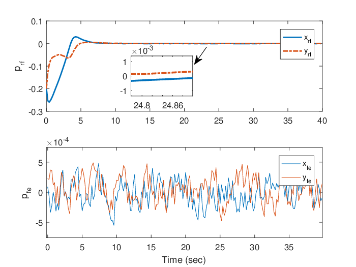
Refer to caption
Figure 3: Tracking errors by using tube-MPC.

First, let us design tube-MPC according to Lemma 3 and Theorem 1. We set the feedback gain to be K=diag​{−2.3,−2.3}K=\rm{diag}\{-2.3,-2.3\}. The control input constraint for Problem 1 is 𝕌t​u​b​e=λt​u​b​e​𝕌\mathbb{U}_{tube}=\lambda_{tube}\mathbb{U} with λt​u​b​e=0.6636\lambda_{tube}=0.6636, and the terminal region is given by Ωt​u​b​e={p~r​f:|x~r​f|+|y~r​f|≤0.0542}\Omega_{tube}=\{\tilde{p}_{rf}:|\tilde{x}_{rf}|+|\tilde{y}_{rf}|\leq 0.0542\}. To evaluate the tracking performance, we take the tracking error pr​fp_{rf} and the real position deviation from the center of the tube pf​ep_{fe} as indexes. Applying Algorithm 1 to the tracking system yields the tracking performance as shown in Fig. 3. It can be found, from Fig. 3, that the tracking error converges to a neighbourhood of the origin, and the trajectory of the follower lies in the tube 𝕋=pf​h∗⊕ℙf​e\mathbb{T}=p_{fh}^{*}\oplus\mathbb{P}_{fe} with ℙf​e={|pf​e|≤[0.00170.0017]}\mathbb{P}_{fe}=\{|p_{fe}|\leq\left[\begin{array}[]{c}0.0017\\ 0.0017\\ \end{array}\right]\}, which is obtained from Lemma 3. Fig. 4 shows the control input performance of the follower. We also take |v|/a+|ω|/b|v|/a+|\omega|/b as an index to evaluate the input constraint. The fluctuated control signal indicates the effectiveness of the feedback part of the controller which reduces the tracking error caused by the disturbances. Furthermore, the input constraint 𝕌t​u​b​e\mathbb{U}_{tube} for the nominal system is active over the interval t∈[0,3]t\in[0,3], while the constraint 𝕌\mathbb{U} for the real system is not active, which indicates the weak control ability.

Refer to caption
Figure 4: Control input of tube-MPC.

To show the effect of different choices of the feedback gain KK on the tracking performance, we set K=diag​{−1,−1}K=\rm{diag}\{-1,-1\} and K=diag​{−4,−4}K=\rm{diag}\{-4,-4\}, respectively, to observe the difference between the actual trajectory and the optimal one. As shown in Fig. 5, increasing of KK reduces the difference of the actual position and the center of the tube and therefore improves the tracking performance.

Refer to caption
Figure 5: Real-time position deviation from the center of the tube pf​ep_{fe} with different feedback gains.

Next, design NRMPC according to Lemma 4.5, Lemma 4.6 and Theorem 2. The input constraint of NRMPC differs from the constraint of tube-MPC and is given by u~f∈𝕌\tilde{u}_{f}\in\mathbb{U} according to Algorithm 2. The terminal region is designed as Ωε={p~r​f:‖p~r​f‖≤0.063}\Omega_{\varepsilon}=\{\tilde{p}_{rf}:\|\tilde{p}_{rf}\|\leq 0.063\}, and consequently ε=0.063\varepsilon=0.063, which satisfies the conditions in Lemma 4.5, Lemma 4.6 and Theorem 2. Fig. 6 presents the tracking performance of Algorithm 2. It can be observed that the tracking error converges to a neighbourhood of the origin. To compare the influence level by disturbances of the two strategies proposed, we define pf​e​(tk)=pf​(tk)−p~f∗​(tk)p_{fe}(t_{k})=p_{f}(t_{k})-\tilde{p}_{f}^{*}(t_{k}) in NRMPC. It can be seen that the tracking performance is directly influenced by disturbances due to the open-loop control during each sampling period. Fig. 7 shows the control input under NRMPC. According to Algorithm 2, the control signal at each time instant is optimal corresponding to its current state, which indicates its robustness. We also note that the input constraint is active over the interval t∈[0,1.5]t\in[0,1.5], which demonstrates a better tracking capability.

Refer to caption
Figure 6: Tracking errors by using NRMPC.
Refer to caption
Figure 7: Control input of NRMPC.

To further compare tube-MPC with NRMPC, we take cost function JJ, real stage cost ‖pr​f‖Q2+‖ur​f‖P2\|p_{rf}\|_{Q}^{2}+\|u_{rf}\|_{P}^{2}, real state cost ‖pr​f‖Q2\|p_{rf}\|_{Q}^{2} and real input cost ‖ur​f‖P2\|u_{rf}\|_{P}^{2} to evaluate the converging performance. Their cost curves are plotted in Fig 8. As it can be seen, the total cost, the stage cost and the state cost decrease faster by implementing NRMPC than by tube-MPC. However, the input cost of NRMPC is higher than that of tube-MPC. This is explained by the fact that the input constraint of tube-MPC is tighter than that of NRMPC, which may degrade the control capability. This also helps explaining why the tracking error decreases faster by NRMPC than by tube-MPC. Fig. 9 provides the computation time in solving the optimization problems. It shows that there is no significant difference between NRMPC and tube-MPC, which implies that they have almost the same computational complexity. However, as stated in Remark 4, the optimization problem can be solved off-line in tube-MPC, whereas the optimization problem has to be solved on-line in NRMPC.

Finally, we summarize the simulation study as follows:

  • (i)

    Tube-MPC presents a better steady state performance than NRMPC. This is because the control strategy of tube-MPC consists of two parts: optimal control and feedback part, while NRMPC is open-loop control during each sampling period.

  • (ii)

    NRMPC performs better in terms of dynamic property than tube-MPC due to the tighter input constraint of tube-MPC.

  • (iii)

    The computational complexities of tube-MPC and NRMPC are almost the same. However, the optimization problem in tube-MPC can be solved off-line, which may enhance its real-time performance.

Refer to caption
Figure 8: Costs of tube-MPC and NRMPC.
Refer to caption
Figure 9: Computation time of tube-MPC and NRMPC.

6 Conclusion

In this paper, two robust MPC strategies have been developed for tracking of nonholonomic systems with coupled input constraint and bounded disturbances. We first developed a tube-MPC strategy, where the trajectory of the real system is constrained in a tube centered along the optimal nominal trajectory by a nonlinear feedback law based on the deviation of the actual states from the optimal nominal states. Tube-MPC possesses robustness but sacrifices optimality, thus we further developed the NRMPC scheme, where the state of the nominal system is updated by the actual state at each step. It was shown that the tracking control system is ISS under both robust MPC strategies, and their optimization problems are feasible. Simulation results illustrated the effectiveness of the two schemes and their respective advantages.

References

  • [1] J. Simanek, M. Reinstein, and V. Kubelka. Evaluation of the EKF-based estimation architectures for data fusion in mobile robots. IEEE/ASME Transactions on Mechatronics, 20(2):985–990, 2015.
  • [2] P. Wang and B. Ding. Distributed RHC for tracking and formation of nonholonomic multi-vehicle systems. IEEE Transactions on Automatic Control, 59(6):1439–1453, 2014.
  • [3] G. Lafferriere, A. Williams, J. Caughman, and J.J.P. Veerman. Decentralized control of vehicle formations. Systems &\& control letters, 54(9):899–910, 2005.
  • [4] Z. P. Jiang and H. Nijmeijer. Tracking control of mobile robots: a case study in backstepping. Automatica, 33(7):1393–1399, 1997.
  • [5] J. Yang and J. Kim. Sliding mode control for trajectory tracking of nonholonomic wheeled mobile robots. IEEE Transactions on Robotics and Automation, 15(3):578–587, 1999.
  • [6] T. Lee, K. Song, C. Lee, and C. Teng. Tracking control of unicycle-modeled mobile robots using a saturation feedback controller. IEEE Transactions on Control Systems Technology, 9(2):305–318, 2001.
  • [7] J. A. Marshall, M. E. Broucke, and B. A. Francis. Pursuit formations of unicycles. Automatica, 42(1):3–12, 2006.
  • [8] J. Ghommam, H. Mehrjerdi, M. Saad, and F. Mnif. Formation path following control of unicycle-type mobile robots. Robotics and Autonomous Systems, 58(5):727–736, 2010.
  • [9] D. Gu and H. Hu. Receding horizon tracking control of wheeled mobile robots. IEEE Transactions on Control Systems Technology, 14(4):743–749, 2006.
  • [10] D. Q. Mayne, J. B. Rawlings, C. V. Rao, and P. O. M. Scokaert. Constrained model predictive control: Stability and optimality. Automatica, 36(6):789–814, 2000.
  • [11] J. Chen, D. Sun, J. Yang, and H. Chen. Leader-follower formation control of multiple nonholonomic mobile robots incorporating receding-horizon scheme. The International Journal of Robotics Research, 29:727–747, 2010.
  • [12] Z. Sun and Y. Xia. Receding horizon tracking control of unicycle-type robots based on virtual structure. International Journal of Robust and Nonlinear Control, 2016, DOI: 10.1002/rnc.3555.
  • [13] J. B. Rawlings and D. Q. Mayne. Model predictive control: Theory and design. Nob Hill Pub., 2009.
  • [14] P. O. M. Scokaert and J. B. Rawlings. Stability of model predictive control under perturbations. In Proceedings of the IFAC Symposium on Nonlinear Control Systems Design, pages 1317–1322, 1995.
  • [15] D. L. Marruedo, T. Alamo, and E. F. Camacho. Stability analysis of systems with bounded additive uncertainties based on invariant sets: Stability and feasibility of MPC. In Proceedings of American Control Conference, pages 364–369, 2002.
  • [16] M. V. Kothare, V. Balakrishnan, and M. Morari. Robust constrained model predictive control using linear matrix inequalities. Automatica, 32(10):1361–1379, 1996.
  • [17] J. H. Lee and Z. Yu. Worst-case formulations of model predictive control for systems with bounded parameters. Automatica, 33(5):763–781, 1997.
  • [18] Z. Wan and M. V. Kothare. Robust output feedback model predictive control using off-line linear matrix inequalities. Journal of Process Control, 12(7):763–774, 2002.
  • [19] L. Magni, G. De Nicolao, R. Scattolini, and F. Allgöwer. Robust model predictive control for nonlinear discrete-time systems. International Journal of Robust and Nonlinear Control, 13(3-4):229–246, 2003.
  • [20] H. Chen, C. W. Scherer, and F. Allgöwer. A game theoretic approach to nonlinear robust receding horizon control of constrained systems. In Proceedings of American control conference, volume 5, pages 3073–3077, 1997.
  • [21] D. Limón, T. Alamo, F. Salas, and E. F. Camacho. Input to state stability of min–max MPC controllers for nonlinear systems with bounded uncertainties. Automatica, 42(5):797–803, 2006.
  • [22] D. M. Raimondo, D. Limon, M. Lazar, L. Magni, and E. F. Ndez Camacho. Min-max model predictive control of nonlinear systems: A unifying overview on stability. European Journal of Control, 15(1):5–21, 2009.
  • [23] D. Q. Mayne and W. Langson. Robustifying model predictive control of constrained linear systems. Electronics Letters, 37(23):1422–1423, 2001.
  • [24] L. Chisci, J. A. Rossiter, and G. Zappa. Systems with persistent disturbances: predictive control with restricted constraints. Automatica, 37(7):1019–1028, 2001.
  • [25] W. Langson, I. Chryssochoos, S. V. Raković, and D. Q. Mayne. Robust model predictive control using tubes. Automatica, 40(1):125–133, 2004.
  • [26] D. Q. Mayne, M. M. Seron, and S. V. Raković. Robust model predictive control of constrained linear systems with bounded disturbances. Automatica, 41(2):219–224, 2005.
  • [27] D. Q. Mayne, E. C. Kerrigan, E. J. Van Wyk, and P. Falugi. Tube-based robust nonlinear model predictive control. International Journal of Robust and Nonlinear Control, 21(11):1341–1353, 2011.
  • [28] S. Yu, C. Maier, H. Chen, and F. Allgöwer. Tube MPC scheme based on robust control invariant set with application to lipschitz nonlinear systems. Systems &\& Control Letters, 62(2):194–200, 2013.
  • [29] J. Fleming, B. Kouvaritakis, and M. Cannon. Robust tube MPC for linear systems with multiplicative uncertainty. IEEE Transactions on Automatic Control, 60(4):1087–1092, 2015.
  • [30] D. L. Marruedo, T. Alamo, and E. F. Camacho. Input-to-state stable MPC for constrained discrete-time nonlinear systems with bounded additive uncertainties. In Proceedings of IEEE Conference on Decision and Control, volume 4, pages 4619–4624, 2002.
  • [31] A. Richards and J. How. Robust stable model predictive control with constraint tightening. In Proceedings of American Control Conference, pages 1557–1562, 2006.
  • [32] H. Li and Y. Shi. Robust distributed model predictive control of constrained continuous-time nonlinear systems: a robustness constraint approach. IEEE Transactions on Automatic Control, 59(6):1673–1678, 2014.
  • [33] E. D. Sontag and Y. Wang. On characterizations of the input-to-state stability property. Systems &\& Control Letters, 24(5):351–359, 1995.
  • [34] H. Michalska and D. Q. Mayne. Robust receding horizon control of constrained nonlinear systems. IEEE Transactions on Automatic Control, 38(11):1623–1633, 1993.
  • [35] P. Falugi, E. Kerrigan, and E. v. Wyk. Imperial college london optimal control software (iclocs). http://www.ee.ic.ac.uk/ICLOCS/.
  • [36] A. Wächter and L. T. Biegler. On the implementation of an interior-point filter line-search algorithm for large-scale nonlinear programming. Mathematical Programming, 106(1):25–57, 2006.
  • [37] F. Mondada, M. Bonani, X. Raemy, J. Pugh, C. Cianci, A. Klaptocz, S. Magnenat, J. Zufferey, D. Floreano, and A. Martinoli. The e-puck, a robot designed for education in engineering. In Proceedings of the 9th conference on autonomous robot systems and competitions, volume 1, pages 59–65, 2009.