Absolute continuity and $\alpha$ -numbers on the real lineThanks: The research was supported by the grants 274512 and 309365 of the Finnish Academy.

Tuomas Orponen Address: University of Helsinki, Department of Mathematics and Statistics Email address: tuomas.orponen@helsinki.fi

Abstract.

Let $\mu,\nu$ be Radon measures on $\mathbb{R}$ , with $\mu$ non-atomic and $\nu$ doubling, and write $\mu=\mu_{a}+\mu_{s}$ for the Lebesgue decomposition of $\mu$ relative to $\nu$ . For an interval $I\subset\mathbb{R}$ , define $\alpha_{\mu,\nu}(I):=\mathbb{W}_{1}(\mu_{I},\nu_{I})$ , the Wasserstein distance of normalised blow-ups of $\mu$ and $\nu$ restricted to $I$ . Let $\mathcal{S}_{\nu}$ be the square function

\mathcal{S}^{2}_{\nu}(\mu)=\sum_{I\in\mathcal{D}}\alpha_{\mu,\nu}^{2}(I)\chi_{I},

where $\mathcal{D}$ is the family of dyadic intervals of side-length at most one. I prove that $\mathcal{S}_{\nu}(\mu)$ is finite $\mu_{a}$ almost everywhere, and infinite $\mu_{s}$ almost everywhere. I also prove a version of the result for a non-dyadic variant of the square function $\mathcal{S}_{\nu}(\mu)$ . The results answer the simplest " $n=d=1"$ case of a problem of J. Azzam, G. David and T. Toro.

2010 Mathematics Subject Classification

42A99 (Primary)

1. Introduction

1.1. Wasserstein distance and $\alpha$ -numbers

In this paper, $\mu$ and $\nu$ are non-zero Radon measures on $\mathbb{R}$ . The measure $\nu$ is generally assumed to be either dyadically doubling or globally doubling. Dyadically doubling means that

(1.1)

\nu(\hat{I})\leq C\nu(I),\quad I\in\mathcal{D},

where $\mathcal{D}$ is the standard family of dyadic intervals, and $\hat{I}$ is the parent of $I$ , that is, the smallest interval in $\mathcal{D}$ strictly containing $I$ . Globally doubling means that $\nu(B(x,2r))\leq C\nu(B(x,r))$ for $x\in\mathbb{R}$ and $r>0$ ; in particular, this implies $\operatorname{spt}\nu=\mathbb{R}$ . The main example for $\nu$ is the Lebesgue measure $\mathcal{L}$ , and the proofs in this particular case would differ little from the ones presented below. No a priori homogeneity is assumed of $\mu$ .

Definition 1.2 (Wasserstein distance).

I will use the following definition of the (first) Wasserstein distance: given two Radon measures measures $\nu_{1},\nu_{2}$ on $[0,1]$ , set

\mathbb{W}_{1}(\nu_{1},\nu_{2}):=\sup_{\psi}\left|\int\psi\,d\nu_{1}-\int\psi\,d\nu_{2}\right|,

where the $\sup$ is taken over all $1$ -Lipschitz functions $\psi\colon\mathbb{R}\to\mathbb{R}$ , which are supported on $[0,1]$ . Such functions will be called test functions. A slightly different – and also quite common – definition would allow the $\sup$ to run over all $1$ -Lipschitz functions $\psi\colon[0,1]\to\mathbb{R}$ . To illustrate the difference, let $\nu_{1}=\delta_{0}$ and $\nu_{2}=\delta_{1}$ . Then $\mathbb{W}_{1}(\nu_{1},\nu_{2})=0$ , but the alternative definition, say $\tilde{\mathbb{W}}_{1}$ , would give $\tilde{\mathbb{W}}_{1}(\nu_{1},\nu_{2})=1$ . The main reason for using $\mathbb{W}_{1}$ instead of $\tilde{\mathbb{W}}_{1}$ in this paper is to comply with the definitions in [1, 2].

As in the paper [1] of J. Azzam, G. David and T. Toro, I make the following definition:

Definition 1.3 ( $\alpha$ -numbers).

Assume that $I\subset\mathbb{R}$ is an interval. Define

\alpha_{\mu,\nu}(I):=\mathbb{W}_{1}(\mu_{I},\nu_{I}),

where $\mu_{I}$ and $\nu_{I}$ are normalised blow-ups of $\mu$ and $\nu$ restricted to $I$ . More precisely, let $T_{I}$ be the increasing affine mapping taking $\overline{I}$ to $[0,1]$ , and define

\mu_{I}:=\frac{T_{I\sharp}(\mu|_{I})}{\mu(I)}\quad\text{and}\quad\nu_{I}:=\frac{T_{I\sharp}(\nu|_{I})}{\nu(I)}.

If $\mu(I)=0$ (or $\nu(I)=0$ ), define $\mu_{I}\equiv 0$ (or $\nu_{I}\equiv 0$ ).

The quantity defined above is somewhat awkward to work with, as it lacks (see Example 5.2) the following desirable stability property: if $I,J\subset\mathbb{R}$ are intervals of comparable length, and $I\subset J$ , then $\alpha_{\mu,\nu}(I)\lesssim\alpha_{\mu,\nu}(J)$ . Chiefly for this reason, I also need to consider the following "smooth" $\alpha$ -numbers; the definition below is essentially the same as the one given by Azzam, David and Toro in [2, Section 5]:

Definition 1.4 (Smooth $\alpha$ -numbers).

Let $\varphi:=\operatorname{dist}(\cdot,\mathbb{R}\setminus(0,1))$ . For an interval $I\subset\mathbb{R}$ , define $\alpha_{s,\mu,\nu}(I):=\mathbb{W}_{1}(\mu_{\varphi,I},\nu_{\varphi,I})$ , where

\mu_{\varphi,I}:=\frac{T_{I\sharp}(\mu|_{I})}{\mu(\varphi_{I})}\quad\text{and}\quad\nu_{\varphi,I}:=\frac{T_{I\sharp}(\nu|_{I})}{\nu(\varphi_{I})}.

Here $T_{I}$ is the map from Definition 1.3, $\varphi_{I}=\varphi\circ T_{I}$ , and $\mu(\varphi_{I})=\int\varphi_{I}\,d\mu$ . If $\mu(\varphi_{I})=0$ (or $\nu(\varphi_{I})=0$ ), set $\mu_{\varphi,I}\equiv 0$ (or $\nu_{\varphi,I}\equiv 0$ ).

The only difference between the numbers $\alpha_{\mu,\nu}(I)$ and $\alpha_{s,\mu,\nu}(I)$ is in the normalisation of the measures $\mu_{I},\varphi_{I}$ and $\mu_{\varphi,I},\nu_{\varphi,I}$ : if $I$ is closed, the measures $\mu_{I},\nu_{I}$ are probability measures on $[0,1]$ , while $\mu_{\varphi,I}([0,1])=\mu(I)/\mu(\varphi_{I})$ . The numbers $\alpha_{s,\mu,\nu}(I)$ enjoy the stability property alluded to above. Moreover, if either $\mu$ or $\nu$ is a doubling, one has $\alpha_{s,\mu,\nu}(I)\lesssim\alpha_{\mu,\nu}(I)$ . These facts are contained in Proposition 5.4 (or see [2, Section 5]).

Remark 1.5.

The $\alpha$ -numbers were first introduced by X. Tolsa in [7], where he used them to characterise the uniform rectifiability of Ahlfors-David regular measures in $\mathbb{R}^{d}$ . Tolsa’s original definition of the $\alpha$ -numbers has a different, asymmetric, normalisation compared to either $\alpha_{\mu,\nu}$ or $\alpha_{s,\mu,\nu}$ above, see [7, p. 394].

1.2. Main results

Before explaining the results in Azzam, David and Toro’s paper [1], and their connection to the current manuscript, I emphasise that [1] treats " $n$ -dimensional" measures in $\mathbb{R}^{d}$ , for any $1\leq n\leq d$ . For the current paper, only the case $n=d=1$ is relevant. So, to avoid digressing too much, I need to state the results of [1] in far smaller generality than they deserve.

With this proviso in mind, the main results of [1] imply the following. if $\mu$ is a doubling measure on $\mathbb{R}$ , and the numbers $\alpha_{\mu,\mathcal{L}}$ satisfy a Carleson condition of the form

(1.6)

\int_{B(x,2r)}\int_{0}^{2r}\alpha_{\mu,\mathcal{L}}(B(y,t))\,\frac{dt\,d\mu y}{t}\leq C\mu(B(x,r)),

then $\mu$ , or at least a large part of $\mu$ , is absolutely continuous with respect to $\mathcal{L}$ , with quantitative upper and lower bounds on the density. As the authors of [1] point out, the main shortcoming of their result is that condition (1.6) imposes a hypothesis on the first powers of the numbers $\alpha_{\mu,\mathcal{L}}$ , whereas evidence suggests (see [1, Remark 1.6.1], the discussion after [1, Theorem 1.7], and [1, Example 4.6]) that the correct power should be two. More support for this belief comes from the following "converse" result of Tolsa [8, Lemma 2.2]: if $\mu$ is a finite Borel measure on $\mathbb{R}$ then

(1.7)

\int_{0}^{\infty}\tilde{\alpha}_{\mu,\mathcal{L}}^{2}(x,r)\frac{dr}{r}<\infty\text{ for }\mathcal{L}\text{ a.e. }x\in\mathbb{R}.

In particular, if $\mu\ll\mathcal{L}$ , then (1.7) holds for $\mu$ almost every $x\in\mathbb{R}$ . I should again mention that this is only the easiest $n=d=1$ case of Tolsa’s result. Here $\tilde{\alpha}_{\mu,\mathcal{L}}$ is a variant of the $\alpha$ -number (in fact the one discussed in Remark 1.5).

The purpose of this paper is to address the problem of Azzam, David and Toro in the simplest case $n=d=1$ . I show that control for the second powers of the $\alpha_{\mu,\mathcal{L}}$ -numbers does guarantee absolute continuity with respect to Lebesgue measure. In fact, the doubling assumption on $\mu$ can be dropped, the Carleson condition (1.6) can be relaxed considerably, and the results remain valid, if $\mathcal{L}$ is replaced by any doubling measure $\nu$ . The results below also contain the "converse" statement, analogous to (1.7).

I prove two variants of the main result: one dyadic, and the other non-dyadic. Here is the dyadic version:

Theorem 1.8.

Let $\mathcal{D}$ be the family of dyadic subintervals of $[0,1)$ , and let $\mu,\nu$ be Borel probability measures on $[0,1)$ . Assume that $\mu$ does not charge the boundaries of intervals in $\mathcal{D}$ , and $\nu$ is dyadically doubling. Write $\mu=\mu_{a}+\mu_{s}$ for the Lebesgue decomposition of $\mu$ relative to $\nu$ , where $\mu_{a}\ll\nu$ and $\mu_{s}\perp\nu$ . Finally, let $\mathcal{S}_{\mathcal{D},\nu}(\mu)$ be the square function

\mathcal{S}^{2}_{\mathcal{D},\nu}(\mu)=\sum_{I\in\mathcal{D}}\alpha_{\mu,\nu}^{2}(I)\chi_{I}.

Then:

(a)

$\mathcal{S}_{\nu}(\mu)$ is finite $\mu_{a}$ almost surely, and
(b)

$\mathcal{S}_{\nu}(\mu)$ is infinite $\mu_{s}$ almost surely.

In particular,

\sum_{I\in\mathcal{D}}\alpha_{\mu,\nu}^{2}(I)\mu(I)<\infty\quad\Longrightarrow\quad\mu\ll\nu.

Heuristically, this corresponds to assuming (1.6) at the scale $r=1$ , but I could not found a way to reduce the continuous problem to the dyadic one; on the other hand, a reduction in the other direction does not appear straightforward, either, so perhaps one needs to treat the cases separately. A caveat of the dyadic set-up is the "non-atomicity" hypothesis on $\mu$ . It cannot be dispensed with: for instance, if $\mu=\delta_{x}$ for any $x\in[0,1)$ , which only belongs to the interiors of finitely many dyadic intervals, then $\mathcal{S}_{\mathcal{D},\mathcal{L}}(\mu)$ is uniformly bounded (for instance $\mathcal{S}_{\mathcal{D},\mathcal{L}}(\delta_{0})\equiv 0$ ), but $\mu\perp\mathcal{L}$ .

Here is the non-dyadic version of the main theorem:

Theorem 1.9.

Assume that $\mu,\nu$ are Radon measures, and $\nu$ is globally doubling. Write $\mu=\mu_{a}+\mu_{s}$ , as in Theorem 1.8. Let $\mathcal{S}_{\nu}$ be the square function

\mathcal{S}^{2}_{\nu}(\mu)(x)=\int_{0}^{1}\alpha_{s,\mu,\nu}^{2}(B(x,r))\,\frac{dr}{r},\qquad x\in\mathbb{R},

defined via the smooth $\alpha$ -numbers $\alpha_{s,\mu,\nu}$ . Then,

(a)

$\mathcal{S}_{\nu}(\mu)$ is finite $\mu_{a}$ almost surely, and
(b)

$\mathcal{S}_{\nu}(\mu)$ is infinite $\mu_{s}$ almost surely.

Recall that $\alpha_{s,\mu,\nu}(B(x,r))\lesssim\alpha_{\mu,\nu}(B(x,r))$ whenever $\nu$ is doubling, such as $\nu=\mathcal{L}$ , see Proposition 5.4. So, Theorem 1.9 has the following corollary:

Corollary 1.10.

If $\mu$ is a Radon measure on $\mathbb{R}$ such that

(1.11)

\int_{0}^{1}\alpha^{2}_{\mu,\mathcal{L}}(B(x,t))\,\frac{dt}{t}<\infty

for $\mu$ almost every $x\in\mathbb{R}$ , then $\mu\ll\nu$ .

The following question remains open:

Question 1.

In the setting of Theorem 1.9, is the square function in (1.11) (with $\mathcal{L}$ replaced by $\nu$ ) finite $\mu_{a}$ almost everywhere?

The difficulties arise from the non-stability of the numbers $\alpha_{\mu,\nu}$ . See [2, Section 5], and in particular [2, Lemma 5.3], for related discussion.

Assuming the full Carleson condition (1.6), and that $\mu$ is globally doubling, the authors of [1] prove something more quantitative than $\mu\ll\mathcal{L}$ ; see in particular [1, Theorem 1.9]. The same ought to be true for the second powers of the $\alpha$ -numbers, and indeed the following result can be easily deduced with the method of the current paper:

Theorem 1.12.

Assume that $\mu,\nu$ are Borel probability measures on $[0,1)$ , both dyadically doubling, and assume that the Carleson condition

(1.13)

\sum_{I\subset J}\alpha_{\mu,\nu}^{2}(I)\mu(I)\leq C\mu(J),\qquad J\in\mathcal{D},

holds for some $C\geq 1$ . Then $\mu$ belongs to $A_{\infty}^{\mathcal{D}}(\nu)$ , the dyadic $A_{\infty}$ class relative to $\nu$ . Similarly, if $\mu,\nu$ are Radon measures on $\mathbb{R}$ , both globally doubling, and the Carleson condition (1.6) holds for the second powers $\alpha^{2}_{\mu,\nu}(B(y,t))$ , then $\mu\in A_{\infty}(\nu)$ .

The a priori doubling assumptions cannot be omitted (that is, they are not implied by the Carleson condition): just consider $\mu=2\chi_{[0,1/2)}\,d\mathcal{L}$ . It is clear that the Carleson condition (1.13) holds for the numbers $\alpha^{2}_{\mu,\mathcal{L}}(I)$ , but nevertheless $\mu\notin A_{\infty}^{\mathcal{D}}(\mathcal{L}|_{[0,1]})$ .

1.3. Outline of the paper, and the main steps of the proofs

The main substance of the paper is proving the dyadic result, Theorem 1.8, and in particular part (b). This work takes up Sections 2-4. The proof of part (a) is simpler, and closely follows a previous argument of Tolsa – namely the one used to prove (1.7). The details (both in the dyadic and continuous settings) are given in Section 6. Modifications required to prove part (b) of the "continuous" Theorem 1.9 are outlined in Section 5.

The proof of Theorem 1.8(b) has three main steps. First, the numbers $\alpha_{\mu,\nu}(I)$ are used to control something analyst-friendlier, namely the following dyadic variants:

(1.14)

\Delta_{\mu,\nu}(I)=\left|\frac{\mu(I_{-})}{\mu(I)}-\frac{\nu(I_{-})}{\nu(I)}\right|.

Here $I_{-}$ stands for the left half of $I$ . This would be simple, if $\chi_{[0,1/2)}$ happened to be one of the admissible test functions $\psi$ in the definition of $\mathbb{W}_{1}$ . It is not, however, and in fact there seems to be no direct (and sufficiently efficient) way to control $\Delta_{\mu,\nu}(I)$ by $\alpha_{\mu,\nu}(I)$ , or even $\alpha_{\mu,\nu}(3I)$ . However, it turns out that the numbers are equivalent at the level of certain Carleson sums over trees; proving this statement is the main content of Section 2.

The numbers $\Delta_{\mu,\nu}(I)$ are well-known quantities: they are the (absolute values of the) coefficients in an orthogonal representation of $\mu$ in terms of $\nu$ -adapted Haar functions, and it is known that they can be used to characterise $A_{\infty}$ . The following theorem is due to S. Buckley [3] from 1993:

Theorem 1.15 (Theorem 2.2(iii) in [3]).

Let $\mu,\nu$ be a dyadically doubling Borel probability measures on $[0,1]$ . Then $\mu\in A_{\infty}^{\mathcal{D}}(\nu)$ , if and only if

(1.16)

\sum_{I\subset J}\Delta^{2}_{\mu,\nu}(I)\mu(I)\leq C\mu(J),\qquad J\in\mathcal{D}.

The result in [3] is only stated for $\nu=\mathcal{L}|_{[0,1]}$ , but the proof works in the greater generality. Note the similarity between the Carleson conditions (1.16) and (1.13): The dyadic part of Theorem 1.12 is, in fact, nothing but a corollary of Buckley’s result, assuming that one knows how to control the numbers $\Delta_{\mu,\nu}(I)$ by the numbers $\alpha_{\mu,\nu}(I)$ at the level of Carleson sums; consequently, the short proof of this half of Theorem 1.12 can be found in Section 2. The continuous version is discussed briefly in Remark 5.19.

Buckley’s result is not applicable for Theorem 1.8: the measure $\mu$ is not dyadically doubling, and the information available is much weaker than the Carleson condition (1.13). Handling these issues constitutes the remaining two steps in the proof: all dyadic intervals are split into trees, where $\mu$ is "tree-doubling" (Section 4), and the absolute continuity of $\mu$ with respect to $\nu$ is studied in each tree separately (Section 3).

1.4. Acknowledgements

I am grateful to Jonas Azzam, David Bate, and Antti Käenmaki and for useful discussions during the preparation of the manuscript. I would also like to thank the referees for good comments, and for asking me to prove parts (a) of Theorems 1.8 and 1.9.

2. Comparison of $\alpha$ -numbers and $\Delta$ -numbers

In this section, $\mu$ and $\nu$ are Borel probability measures on $[0,1)$ , $\mu$ does not charge the boundaries of dyadic intervals, and $\nu$ is dyadically doubling inside $[0,1)$ :

\nu(\hat{I})\leq D_{\nu}\nu(I),\qquad I\in\mathcal{D}\setminus\{[0,1)\}.

This implies, in particular, that $\nu(I)>0$ for all $I\in\mathcal{D}$ with $I\subset[0,1)$ . The main task of the section is to bound the numbers $\Delta_{\mu,\nu}(I)$ by the numbers $\alpha_{\mu,\nu}(I)$ , where $\Delta_{\mu,\nu}(I)$ was the quantity

\Delta_{\mu,\nu}(I)=\left|\frac{\mu(I_{-})}{\mu(I)}-\frac{\nu(I_{-})}{\nu(I)}\right|=\left|\int\chi_{(0,1/2)}\,d\mu_{I}-\int\chi_{(0,1/2)}\,d\nu_{I}\right|.

The task would be trivial, if $\chi_{(0,1/2)}$ were a $1$ -Lipschitz function vanishing at the boundary of $[0,1]$ . It is not: in fact, the difference between $\Delta_{\nu_{1},\nu_{2}}(I)$ and $\alpha_{\nu_{1},\nu_{2}}(I)$ can be rather large for a given interval $I$ .

Example 2.1.

If $\nu_{1}=\delta_{1/2-1/n}$ and $\nu_{2}=\delta_{1/2+1/n}$ , then $\Delta_{\nu_{1},\nu_{2}}([0,1))=1$ , but $\alpha_{\nu_{1},\nu_{2}}([0,1))\lesssim 1/n$ . These measures do not satisfy the assumptions of the section, so consider also the following example. Let $\mu=f\,d\mathcal{L}$ , where $f$ takes the value $1$ everywhere, except in the $2^{-n}$ -neighbourhood of $1/2$ . Let $f\equiv 1/2$ on the interval $[1/2-2^{-n},1/2]$ , and $f\equiv 3/2$ on the interval $(1/2,1/2+2^{-n}]$ . Then $\mu$ is dyadically $4$ -doubling probability measure on $[0,1]$ , $\Delta_{\mu,\mathcal{L}}([0,1))\sim 2^{-n}$ , and $\alpha_{\mu,\mathcal{L}}([0,1))\sim 2^{-2n}$ .

Fortunately, "pointwise" estimates between $\Delta_{\mu,\nu}(I)$ and $\alpha_{\mu,\nu}(I)$ are not really needed in this paper, and it turns out that certain sums of these numbers are comparable, up to a manageable error. To state such results, I need to introduce some terminology. A family $\mathcal{C}\subset\mathcal{D}$ of dyadic intervals is called coherent, if the implication

Q,R\in\mathcal{C}\text{ and }Q\subset P\subset R\quad\Longrightarrow\quad P\in\mathcal{C}

holds for all $Q,P,R\in\mathcal{D}$ .

Definition 2.2 (Trees, leaves, boundary).

A tree $\mathcal{T}\subset\mathcal{D}$ is any coherent family of dyadic intervals with a unique largest interval, $\mathbf{Top}(\mathcal{T})\in\mathcal{T}$ , and with the property that

\operatorname{card}(\mathbf{ch}(I)\cap\mathcal{T})\in\{0,2\},\qquad I\in\mathcal{T}.

For the tree $\mathcal{T}$ , define the set family $\mathbf{Leaves}(\mathcal{T})$ to consist of the minimal intervals in $\mathcal{T}$ , in other words those $I\in\mathcal{T}$ with $\operatorname{card}(\mathbf{ch}(I)\cap\mathcal{T})=0$ . Abusing notation, I often write $\mathbf{Leaves}(\mathcal{T})$ also for the set $\cup\{I:I\in\mathbf{Leaves}(\mathcal{T})\}$ . Finally, define the boundary of the tree $\partial\mathcal{T}$ by

\partial T:=\mathbf{Top}(\mathcal{T})\setminus\mathbf{Leaves}(\mathcal{T}).

Then $x\in\partial\mathcal{T}$ , if and only if $x\in\mathbf{Top}(\mathcal{T})$ , and all intervals $I\in\mathcal{D}$ with $x\in I\subset\mathbf{Top}(\mathcal{T})$ are contained $\mathcal{T}$ .

Definition 2.3 ( $(\mathcal{T},D)$ -doubling measures).

A Borel probability measure $\mu$ on $[0,1]$ is called $(\mathcal{T},D)$ -doubling, if

\mu(\hat{I})\leq D\mu(I),\qquad I\in\mathcal{T}\setminus\mathbf{Top}(\mathcal{T}).

Here is the main result of this section:

Proposition 2.4.

Let $\mu,\nu$ be measures satisfying the assumptions of the section, and let $\mathcal{T}\subset\mathcal{D}$ be a tree. Moreover, assume that $\mu$ is $(\mathcal{T},D)$ -doubling for some constant $D\geq 1$ . Then

\sum_{I\in\mathcal{T}}\Delta_{\mu,\nu}^{2}(I)\mu(I)\lesssim_{D_{\nu},D}\sum_{I\in\mathcal{T}\setminus\mathbf{Leaves}(\mathcal{T})}\alpha_{\mu,\nu}^{2}(I)\mu(I)+\mu(\mathbf{Top}(\mathcal{T})).

The "dyadic part" of Theorem 1.12 is an immediate corollary:

Proof of Theorem 1.12, dyadic part.

By hypothesis, both measures $\mu$ and $\nu$ are $(\mathcal{D},C)$ -doubling. Hence, by the Carleson condition (1.13), and Proposition 2.4 applied to the trees $\mathcal{T}_{J}:=\{I\in\mathcal{D}:I\subset J\}$ , one has

\sum_{I\subset J}\Delta_{\mu,\nu}^{2}(I)\mu(I)\lesssim_{C}\sum_{I\subset J}\alpha_{\mu,\nu}^{2}(I)\mu(I)+\mu(J)\lesssim\mu(J).

This is precisely the condition in Buckley’s result, Theorem 1.15, so $\mu\in A^{\mathcal{D}}_{\infty}(\nu)$ . ∎

I then begin the proof of Proposition 2.4. It would, in fact, suffice to assume that $\nu$ is also just $(\mathcal{T},D_{\nu})$ -doubling, but checking this would result in some unnecessary book-keeping below. The proof is based on the observation that $\chi_{(0,1/2)}$ can be written as a series of Lipschitz functions, each supported on sub-intervals of $[0,1]$ . This motivates the following considerations.

Assume that

\Psi:=\Psi_{0}:=\sum_{j\geq 0}\psi_{j}

is a bounded function such that each $\psi_{j}\colon\mathbb{R}\to[0,\infty)$ is an $L_{j}$ -Lipschitz function supported on some interval $I_{j}\in\mathcal{D}_{j}$ . Assume moreover that the intervals $I_{j}$ are nested: $[0,1)\supset I_{1}\supset I_{2}\ldots$ . Then, as a first step in proving Proposition 2.4, I claim that

(2.5)		$\displaystyle\left\|\int\Psi\,d\mu-\int\Psi\,d\nu\right\|$	$\displaystyle\leq\sum_{k=0}^{N}\frac{L_{k}}{2^{k}}\alpha_{\mu,\nu}(I_{k})\mu(I_{k})$
		$\displaystyle+\sum_{k=0}^{N}\left(\frac{1}{\nu(I_{k+1})}\int\Psi_{k+1}\,d\nu\right)\Delta_{\mu,\nu}(I_{k})\mu(I_{k})+2\\|\Psi\\|_{\infty}\mu(I_{N+1})$

for any $N\in\{0,1,\ldots,\infty\}$ , where

\Psi_{k}:=\sum_{j\geq k}\psi_{j},\qquad m\geq 0.

For $N=\infty$ , the symbol " $I_{N+1}$ " should be interpreted as the intersection of all the intervals $I_{j}$ . I will first verify that, for any $m\geq 0$ ,

	$\displaystyle\left\|\frac{1}{\mu(I_{m})}\int\Psi_{m}\,d\mu-\frac{1}{\nu(I_{m})}\int\Psi_{m}\,d\nu\right\|$
(2.6)		$\displaystyle\leq\frac{L_{m}}{2^{m}}\alpha_{\mu,\nu}(I_{m})+\left(\frac{1}{\nu(I_{m+1})}\int\Psi_{m+1}\,d\nu\right)\Delta_{\mu,\nu}(I_{m})$
	$\displaystyle\quad+\frac{\mu(I_{m+1})}{\mu(I_{m})}\left\|\frac{1}{\mu(I_{m+1})}\int\Psi_{m+1}\,d\mu-\frac{1}{\nu(I_{m+1})}\int\Psi_{m+1}\,d\nu\right\|$

from which it will be easy to derive (2.5). If $\mu(I_{m})=0$ , the corresponding term should be interpreted as " $0$ " (recall that $\nu(I_{m})$ is never zero by the doubling assumption). The proof of (2.6) is straightforward. First, note that since $\psi_{m}\colon\mathbb{R}\to\mathbb{R}$ is an $L_{m}$ -Lipschitz function supported on $I_{m}$ , and $|I_{m}|=2^{-m}$ , one has

\left|\frac{1}{\mu(I_{m})}\int\psi_{m}\,d\mu-\frac{1}{\nu(I_{m})}\int\psi_{m}\,d\nu\right|=\left|\int\psi_{m}\circ T_{I_{m}}^{-1}\,d\mu_{I_{m}}-\int\psi_{m}\circ T_{I_{m}}^{-1}\,d\nu_{I_{m}}\right|\leq\frac{L_{m}}{2^{m}}\alpha_{\mu,\nu}(I_{m}).

(The mappings $T_{I}$ are familiar from Definition 1.3). This gives rise to the first term in (2.6). What remains is bounded by

		$\displaystyle\left\|\frac{1}{\mu(I_{m})}\int\Psi_{m+1}\,d\mu-\frac{1}{\nu(I_{m})}\int\Psi_{m+1}\,d\nu\right\|$
		$\displaystyle\leq\frac{\mu(I_{m+1})}{\mu(I_{m})}\left\|\frac{1}{\mu(I_{m+1})}\int\Psi_{m+1}\,d\mu-\frac{1}{\nu(I_{m+1})}\int\Psi_{m+1}\,d\nu\right\|$
		$\displaystyle\quad+\left(\frac{1}{\nu(I_{m+1})}\int\Psi_{m+1}\,d\nu\right)\left\|\frac{\mu(I_{m+1})}{\mu(I_{m})}-\frac{\nu(I_{m+1})}{\nu(I_{m})}\right\|.$

This is (2.6), observing that

\Delta_{\mu,\nu}(I_{m})=\left|\frac{\mu(I_{m+1})}{\mu(I_{m})}-\frac{\nu(I_{m+1})}{\nu(I_{m})}\right|,

since either $I_{m+1}=(I_{m})_{+}$ or $I_{m+1}=(I_{m})_{-}$ , and both possibilities give the same number $\Delta_{\mu,\nu}(I_{m})$ . Finally, (2.5) is obtained by repeated application of (2.6). By induction, one can check that $N$ iterations of (2.6) (starting from $m=0$ , and recalling that $\mu,\nu$ are probability measures on $[0,1)$ ) leads to

		$\displaystyle\left\|\int\Psi\,d\mu-\int\Psi\,d\nu\right\|\leq\sum_{k=0}^{N}\frac{L_{k}}{2^{k}}\alpha_{\mu,\nu}(I_{k})\mu(I_{k})+\sum_{k=0}^{N}\left(\frac{1}{\nu(I_{k+1})}\int\Psi_{k+1}\,d\nu\right)\Delta_{\mu,\nu}(I_{k})\mu(I_{k})$
(2.7)			$\displaystyle\qquad+\mu(I_{N+1})\left\|\frac{1}{\mu(I_{N+1})}\int\Psi_{N+1}\,d\mu-\frac{1}{\nu(I_{N+1})}\int\Psi_{N+1}\,d\nu\right\|.$

This gives (2.5) immediately, observing that $\|\Psi_{N+1}\|_{\infty}\leq\|\Psi\|_{\infty}$ .

Now, it is time to specify the functions $\psi_{j}$ . I first define a hands-on Whitney decomposition for $(0,1/2)$ . Pick a small parameter $\tau>0$ , to be specified later, and let $U_{0}:=[\tau,1/2-\tau)$ . Then, set $U_{-k}:=[\tau 2^{-k},\tau 2^{-k+1})$ and $U_{k}:=1/2-U_{-k}$ for $k\geq 1$ . Let $\{\psi_{k}\}_{k\in\mathbb{Z}}$ be a partition of unity subordinate to slightly enlarged versions of the sets $U_{k}$ , $k\in\mathbb{Z}$ . By this, I first mean that each $\psi_{k}$ is non-negative and $L_{k}$ -Lipschitz with

(2.8)

L_{k}\leq\frac{C2^{|k|}}{\tau}.

Second, the supports of the functions $\psi_{k}$ should satisfy $\psi_{0}\subset[\tau/2,1/2-\tau/2)$ ,

\operatorname{spt}\psi_{-k}\subset[(\tau/2)2^{-k},2\tau 2^{-k+1})\subset(0,2\tau 2^{-k+1})\quad\text{and}\quad\psi_{k}\subset 1/2-(0,2\tau 2^{-k+1})

for $k\geq 1$ . Third,

\sum_{k\in\mathbb{Z}}\psi_{k}=\chi_{(0,1/2)}.

Let $\Psi^{-}:=\sum_{k>0}\psi_{-k}+\psi_{0}/2$ and $\Psi^{+}:=\sum_{k>0}\psi_{k}+\psi_{0}/2$ . Then

(2.9)

\Delta_{\mu,\nu}([0,1))\leq\left|\int\Psi^{-}\,d\mu-\int\Psi^{-}\,d\nu\right|+\left|\int\Psi^{+}\,d\mu-\int\Psi^{+}\,d\nu\right|.

This is the only place in the paper, where the assumption of $\mu$ not charging the boundaries of dyadic intervals is used (however, the estimate (2.9) will eventually be applied to all the measures $\mu_{I}$ , $I\in\mathcal{D}$ , so the full strength of the hypothesis is needed). The function $\Psi^{-}$ is precisely of the form treated above with $I_{j}:=[0,2^{-j})$ , since clearly $\operatorname{spt}\psi_{-k}\subset I_{k}$ . Applying the inequality (2.5) with any $N_{1}\in\{0,1,\ldots,\infty\}$ yields

(2.10)		$\displaystyle\left\|\int\Psi^{-}\,d\mu-\int\Psi^{-}\,d\nu\right\|$	$\displaystyle\leq\sum_{k=0}^{N_{1}}\frac{L_{-k}}{2^{k}}\alpha_{\mu,\nu}(I_{k})\mu(I_{k})$
		$\displaystyle+\sum_{k=0}^{N_{1}}\left(\frac{1}{\nu(I_{k+1})}\int\Psi^{-}_{k+1}\,d\nu\right)\Delta_{\mu,\nu}(I_{k})\mu(I_{k})+2\mu(I_{N_{1}+1}).$

Next, observe that each function $\Psi^{-}_{k+1}$ , $k\geq 0$ , is bounded by $1$ and vanishes outside

\bigcup_{j=k+1}^{\infty}\operatorname{spt}\psi_{-k}\subset(0,2\tau 2^{-k}).

It follows that

\frac{1}{\nu(I_{k+1})}\int\Psi^{-}_{k+1}\,d\nu\leq\frac{\nu((0,2\tau 2^{-k}))}{\nu(I_{k+1})}=o_{D_{\nu}}(\tau),

where the implicit constants only depend on the dyadic doubling constant $D_{\nu}$ of $\nu$ . In the sequel, I assume that $\tau$ is so small that $o_{D_{\nu}}(\tau)\leq\kappa$ , where $\kappa>0$ is another small constant, which will eventually depend on the $(\mathcal{T},D)$ -doubling constant $D$ for $\mu$ . Recalling also (2.8), the estimate (2.10) then becomes

(2.11)

\left|\int\Psi^{-}\,d\mu-\int\Psi^{-}\,d\nu\right|\leq\frac{C}{\tau}\sum_{k=0}^{N_{1}}\alpha_{\mu,\nu}(I_{k})\mu(I_{k})+\kappa\sum_{k=0}^{N_{1}}\Delta_{\mu,\nu}(I_{k})\mu(I_{k})+2\mu(I_{N_{1}+1}).

The last term simply vanishes, if $N_{1}=\infty$ , because $\mu(\{0\})=0$ . A heuristic point to observe is that the left hand side is roughly $\Delta_{\mu,\nu}([0,1])$ ; the right hand side also contains the same term, but multiplied by a small constant $\kappa>0$ . This gain is "paid for" by the large constant $C/\tau$ .

Next, the estimate is replicated for $\Psi^{+}$ . This time, the inequality (2.5) is applied to the sequence $\tilde{I}_{0}=[0,1)$ , $\tilde{I}_{1}=[0,1/2)$ , $\tilde{I}_{2}=(\tilde{I}_{1})_{+}$ , and in general $\tilde{I}_{k+1}=(\tilde{I}_{k})_{+}$ for $k\geq 1$ (here $J_{+}$ is the right half of $J$ ). Then, if $\tau$ is small enough, it is again clear that $\operatorname{spt}\psi_{k}\subset\tilde{I}_{k}$ . Thus, by inequality (2.5),

(2.12)		$\displaystyle\left\|\int\Psi^{+}\,d\mu-\int\Psi^{+}\,d\nu\right\|$	$\displaystyle\leq\sum_{k=0}^{N_{2}}\frac{L_{k}}{2^{k}}\alpha_{\mu,\nu}(\tilde{I}_{k})\mu(\tilde{I}_{k})$
		$\displaystyle+\sum_{k=0}^{N_{2}}\left(\frac{1}{\nu(\tilde{I}_{k+1})}\int\Psi^{+}_{k+1}\,d\nu\right)\Delta_{\mu,\nu}(\tilde{I}_{k})\mu(\tilde{I}_{k})+2\mu(\tilde{I}_{N_{2}+1})$

for any $N_{2}\geq 0$ . As before, the term $\mu(\tilde{I}_{N_{2}})$ vanishes for $N_{2}=\infty$ (because $\mu(\{\tfrac{1}{2}\})=0$ ), and one can ensure

\frac{1}{\nu(\tilde{I}_{k+1})}\int\Psi^{+}_{k+1}\,d\nu\leq\kappa

by choosing $\tau=\tau(D_{\nu})>0$ small enough. Consquently (recalling (2.9)), (2.11) and (2.12) together imply

(2.13)

\Delta_{\mu,\nu}([0,1))\leq\frac{C}{\tau}\sum_{I\in\mathbf{Tail}}\alpha_{\mu,\nu}(I)\mu(I)+\kappa\sum_{I\in\mathbf{Tail}}\Delta_{\mu,\nu}(I)\mu(I)+2\mu(I_{N_{1}+1})+2\mu(\tilde{I}_{N_{2}+1}).

Here $\mathbf{Tail}$ is the collection of all the intervals $I_{0},\ldots,I_{N_{1}}$ and $\tilde{I}_{0},\ldots,\tilde{I}_{N_{2}}$ . The intervals $[0,1)$ and $[0,1/2)$ arise a total of two times from (2.11) and (2.12), but this has no visible impact on the end result, (2.13).

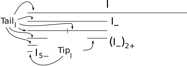
Refer to caption — Figure 1. An example of $\mathbf{Tail}_{I}(4,1)$ and $\mathbf{Tip}_{I}$ .

The estimate (2.13) generalises in a simple way to other intervals $I\in\mathcal{D}$ , besides $I=[0,1)$ , but requires an additional piece of notation. Let $I\in\mathcal{D}$ , and write $I_{0-}:=I=:I_{0+}$ . For $k\geq 1$ , define $I_{k-}:=(I_{(k-1)-})_{-}$ and $I_{k+}:=(I_{(k-1)+})_{+}$ . Now, for a fixed dyadic interval $I\subset[0,1)$ , and $N_{1},N_{2}\geq 0$ , let $\mathbf{Tail}_{I}=\mathbf{Tail}_{I}(N_{1},N_{2})$ be the collection of subintervals of $I$ , which includes $I_{k-}$ for all $0\leq k\leq N_{1}$ and $(I_{-})_{k+}$ for all $0\leq k\leq N_{2}$ , see Figure 1. Then, the generalisation of (2.13) reads

(2.14)

\Delta_{\mu,\nu}(I)\mu(I)\leq\frac{C}{\tau}\sum_{J\in\mathbf{Tail}_{I}}\alpha_{\mu,\nu}(J)\mu(J)+\kappa\sum_{J\in\mathbf{Tail}_{I}}\Delta_{\mu,\nu}(J)\mu(J)+2\mu(\mathbf{Tip}_{I}),

where $\mathbf{Tip}_{I}=I_{(N_{1}+1)-}\cup(I_{-})_{(N_{2}+1)+}$ . If $N_{1}<\infty$ and $N_{2}=\infty$ , for instance, then $\mathbf{Tip}_{I}=I_{(N_{1}+1)-}$ . The proof is nothing but an application of (2.13) to the measures $\mu_{I}$ and $\nu_{I}$ . For minor technical reasons, I also wish to allow the choice $N_{1}=0$ and $N_{2}=-1$ : by definition, this choice means that $\mathbf{Tail}_{I}=\{I\}$ and $\mathbf{Tip}_{I}:=I_{-}$ . It is easy to see that (2.14) remains valid in this case, with " $2$ " replaced by " $4$ " (for $I=[0,1)$ , this follows by applying (2.11) and (2.12) with the choices $N_{1}=0=N_{2}$ ).

Now, the table is set to prove Proposition 2.4, which I recall here:

Proposition 2.15.

\sum_{I\in\mathcal{T}}\Delta_{\mu,\nu}^{2}(I)\mu(I)\lesssim_{D_{\nu},D}\sum_{I\in\mathcal{T}\setminus\mathbf{Leaves}(\mathcal{T})}\alpha_{\mu,\nu}^{2}(I)\mu(I)+\mu(\mathbf{Top}(\mathcal{T})).

Proof.

The sum over $I\in\mathbf{Leaves}(\mathcal{T})$ is evidently bounded by $4\mu(\mathbf{Top}(\mathcal{T}))$ , so it suffices to consider

I\in\mathcal{T}\setminus\mathbf{Leaves}(\mathcal{T})=:\mathcal{T}^{-}.

Let $I\in\mathcal{T}$ , and define the number $N_{1}=N_{1}(I)\geq 0$ as the smallest index so that $I_{(N_{1}+1)-}\in\mathbf{Leaves}(\mathcal{T})$ . If no such index exists, set $N_{1}=\infty$ . If $I_{-}\in\mathbf{Leaves}(\mathcal{T})$ , then $N_{1}=0$ , and I define $N_{2}=-1$ : then $\mathbf{Tail}_{I}:=\{I\}$ , and $\mathbf{Tip}_{I}:=I_{-}$ . Otherwise, if $I_{-}\in\mathcal{T}^{-}$ , let $N_{2}\geq 0$ be the smallest index such that $(I_{-})_{(N_{2}+1)+}\in\mathbf{Leaves}(\mathcal{T})$ . If no such index exists, let $N_{2}=\infty$ . Now $\mathbf{Tail}_{I}\subset\mathcal{T}^{-}$ and $\mathbf{Tip}_{I}\subset\mathbf{Leaves}(\mathcal{T})$ are defined as after (2.14). Start by the following combination of (2.14) and Cauchy-Schwarz:

	$\displaystyle\Delta_{\mu,\nu}^{2}(I)\mu(I)^{2}$	$\displaystyle\lesssim\frac{1}{\tau^{2}}\left(\sum_{J\in\mathbf{Tail}_{I}}\alpha_{\mu,\nu}^{2}(J)\mu(J)^{3/2}\right)\left(\sum_{J\in\mathbf{Tail}_{I}}\mu(J)^{1/2}\right)$
(2.16)			$\displaystyle+\kappa^{2}\left(\sum_{J\in\mathbf{Tail}_{I}}\Delta_{\mu,\nu}^{2}(J)\mu(J)^{3/2}\right)\left(\sum_{J\in\mathbf{Tail}_{I}}\mu(J)^{1/2}\right)+\mu(\mathbf{Tip}_{I})^{2}.$

The factors $\sum_{J\in\mathbf{Tail}_{I}}\mu(J)^{1/2}$ are under control, thanks to the $(\mathcal{T},D)$ -doubling hypothesis on $\mu$ , and the fact that $\mathbf{Tail}_{I}\subset\mathcal{T}$ . Since $\mathbf{Tail}_{I}$ consists of two "branches" of nested intervals inside $I$ , and the $(\mathcal{T},D)$ -doubling hypothesis implies that the $\mu$ -measures of intervals decay geometrically along these branches, one arrives at

\sum_{J\in\mathbf{Tail}_{I}}\mu(J)^{1/2}\lesssim_{D}\mu(I)^{1/2}.

Thus, by (2.16),

(2.17)

\Delta_{\mu,\nu}^{2}(I)\mu(I)\lesssim_{D}\frac{1}{\tau^{2}}\sum_{J\in\mathbf{Tail}_{I}}\alpha_{\mu,\nu}^{2}(J)\frac{\mu(J)^{3/2}}{\mu(I)^{1/2}}+\kappa^{2}\sum_{J\in\mathbf{Tail}_{I}}\Delta_{\mu,\nu}^{2}(J)\frac{\mu(J)^{3/2}}{\mu(I)^{1/2}}+\frac{\mu(\mathbf{Tip}_{I})^{2}}{\mu(I)}.

The constant $\kappa>0$ will have to be chosen so small, eventually, that its product with the implicit constants above is notably less than one. From now on, the precise restriction $J\in\mathbf{Tail}_{I}$ can be replaced by the conditions $J\in\mathcal{T}^{-}$ and $J\subset I$ . With this in mind, observe first that

	$\displaystyle\sum_{I\in\mathcal{T}^{-}}\mathop{\sum_{J\in\mathcal{T}^{-}}}_{J\subset I}\alpha_{\mu,\nu}^{2}(J)\frac{\mu(J)^{3/2}}{\mu(I)^{1/2}}$	$\displaystyle=\sum_{J\in\mathcal{T}^{-}}\alpha_{\mu,\nu}^{2}(J)\mu(J)^{3/2}\mathop{\sum_{I\in\mathcal{T}^{-}}}_{I\supset J}\frac{1}{\mu(I)^{1/2}}$
		$\displaystyle\lesssim_{D}\sum_{J\in\mathcal{T}^{-}}\alpha_{\mu,\nu}^{2}(J)\mu(J).$

The final inequality uses, again, the geometric decay of $\mu$ -measures of intervals in $\mathcal{T}$ . A similar estimate can be performed for the second term in (2.17). As for the third term,

	$\displaystyle\sum_{I\in\mathcal{T}^{-}}\frac{\mu(\mathbf{Tip}_{I})^{2}}{\mu(I)}$	$\displaystyle\lesssim\sum_{I\in\mathcal{T}^{-}}\frac{\mu(I_{(N_{1}+1)-})^{2}+\mu((I_{-})_{(N_{2}+1)+})^{2}}{\mu(I)}$
		$\displaystyle\lesssim\sum_{J\in\mathbf{Leaves}(\mathcal{T})}\mu(J)^{2}\mathop{\sum_{I\in\mathcal{T}^{-}}}_{I\supset J}\frac{1}{\mu(I)}\lesssim_{D}\mu(\mathbf{Leaves}(\mathcal{T})),$

relying once more on the geometric decay of $\mu$ in $\mathcal{T}$ . Combining all the estimates gives

(2.18)

\sum_{I\in\mathcal{T}^{-}}\Delta_{\mu,\nu}^{2}(I)\mu(I)\lesssim_{D}\frac{1}{\tau^{2}}\sum_{I\in\mathcal{T}^{-}}\alpha_{\mu,\nu}^{2}(I)\mu(I)+\kappa^{2}\sum_{I\in\mathcal{T}^{-}}\Delta_{\mu,\nu}^{2}(I)\mu(I)+\mu(\mathbf{Leaves}(\mathcal{T})).

If the left hand side is a priori finite, the proof of Proposition 2.4 is now completed by choosing $\kappa$ small enough, depending on $D$ . If not, consider any finite sub-tree $\mathcal{T}_{j}\subset\mathcal{T}$ with $\mathbf{Top}(\mathcal{T}_{j})=\mathbf{Top}(\mathcal{T})$ . Then, the proof above gives (2.18) with $\mathcal{T}_{j}$ in place of $\mathcal{T}$ . Hence

\sum_{I\in\mathcal{T}_{j}^{-}}\Delta_{\mu,\nu}^{2}(I)\mu(I)\lesssim_{D}\sum_{I\in\mathcal{T}_{j}^{-}}\alpha_{\mu,\nu}^{2}(I)\mu(I)+\mu(\mathbf{Top}(\mathcal{T})),

where the constants do not depend on the choice of $\mathcal{T}_{j}$ . Now the proposition follows by letting $\mathcal{T}_{j}\nearrow\mathcal{T}$ . ∎

3. Absolute continuity of tree-adapted measures

Recall the concepts of tree, leaves and boundaries from Definition 2.2, and the notion of $(\mathcal{T},D)$ -doubling measures from Definition 2.3. In the present section, I assume that $\mathcal{T}\subset\mathcal{D}$ is a tree, and $\mu,\nu$ are two finite Borel measures, which satisfy the following two assumptions:

(A)

$\min\{\mu(\mathbf{Top}(\mathcal{T})),\nu(\mathbf{Top}(\mathcal{T}))\}>0$ , and
(B)

$\mu,\nu$ are $(\mathcal{T},D)$ -doubling for some constant $D\geq 1$ .

In particular, the assumptions imply that

\mu(I)>0\quad\text{and}\quad\nu(I)>0,\qquad I\in\mathcal{T}.

For reasons to become apparent soon, I define the $(\mathcal{T},\mu)$ -adaptation of $\nu$ ,

\nu_{\mathcal{T}}:=\nu|_{\partial\mathcal{T}}+\sum_{I\in\mathbf{Leaves}(\mathcal{T})}\tfrac{\nu}{\mu}(I)\cdot\mu|_{I},

where $\tfrac{\nu}{\mu}(I):=\nu(I)/\mu(I)$ . Note that

(3.1)

\nu_{\mathcal{T}}(I)=\nu(I),\qquad I\in\mathcal{T},

because $\partial\mathcal{T}$ is disjoint from the leaves, which are also pairwise disjoint. In particular, $\nu_{\mathcal{T}}(\mathbf{Top}(\mathcal{T}))=\nu(\mathbf{Top}(\mathcal{T}))$ . The main result of the section is the following:

Proposition 3.2.

Assume (A) and (B), and that

\sum_{I\in\mathcal{T}\setminus\mathbf{Leaves}(\mathcal{T})}\Delta_{\mu,\nu}^{2}(I)\mu(I)<\infty.

Then $\mu|_{\mathbf{Top}(\mathcal{T})}\ll\nu_{\mathcal{T}}$ . In particular $\mu|_{\partial\mathcal{T}}\ll\nu$ .

Remark 3.3.

By the definition of $\nu_{\mathcal{T}}$ , it is obvious that $\mu|_{\mathbf{Leaves}(\mathcal{T})}\ll\nu_{\mathcal{T}}$ . So, the main point of Proposition 3.2 is to show that $\mu|_{\partial\mathcal{T}}\ll(\nu_{\mathcal{T}})|_{\partial\mathcal{T}}=\nu|_{\partial\mathcal{T}}$ .

Since $\mu(\mathbf{Top}(\mathcal{T}))>0$ and $\nu(\mathbf{Top}(\mathcal{T}))>0$ , one may assume without loss of generality that

\mu(\mathbf{Top}(\mathcal{T}))=1=\nu(\mathbf{Top}(\mathcal{T})).

The proof of Proposition 3.2 is based on a "product representation" for $\nu_{\mathcal{T}}$ , relative to $\mu$ , in the spirit of [4, Theorem 3.22] of Fefferman, Kenig and Pipher. Recall that every interval $I\in\mathcal{D}$ has exactly two children: $I_{-}$ and $I_{+}$ . Define the $\mu$ -adapted Haar functions

h_{I}^{\mu}:=c_{I}^{+}\chi_{I_{+}}-c_{I}^{-}\chi_{I_{-}},\qquad I\in\mathcal{T}\setminus\mathbf{Leaves}(\mathcal{T}),

where

c_{I}^{+}:=\frac{\mu(I)}{\mu(I_{+})}\quad\text{and}\quad c_{I}^{-}:=\frac{\mu(I)}{\mu(I_{-})}.

This ensures that $\int h_{I}^{\mu}\,d\mu=0$ for $I\in\mathcal{T}\setminus\mathbf{Leaves}(\mathcal{T})$ . Note that $\mu(I_{+}),\mu(I_{-})>0$ , because $I_{+},I_{-}\in\mathcal{T}$ . Now, the plan is to define coefficients $a_{J}\in\mathbb{R}$ , for $J\in\mathcal{T}\setminus\mathbf{Leaves}(\mathcal{T})$ , so that the following requirement is met:

(3.4)

\mathop{\prod_{J\supsetneq I}}_{J\in\mathcal{T}}(1+a_{J}h_{J}^{\mu})(x)=\tfrac{\nu}{\mu}(I),\qquad x\in I\in\mathcal{T}.

The left hand side of (3.4) is certainly constant on $I$ , so the equation has some hope; if $I=\mathbf{Top}(\mathcal{T})$ , then the product is empty, and the right hand side of (3.4) equals $1$ by the assumption $\mu(\mathbf{Top}(\mathcal{T}))=\nu(\mathbf{Top}(\mathcal{T}))=1$ . Now, assume that (3.4) holds for some interval $I\in\mathcal{T}\setminus\mathbf{Leaves}(\mathcal{T})$ . Then $I_{-},I_{+}\in\mathcal{T}$ , so if (3.4) is supposed to hold for $I_{-}$ , one has

(3.5)

\tfrac{\nu}{\mu}(I_{-})=\mathop{\prod_{J\supsetneq I_{-}}}_{J\in\mathcal{T}}(1+a_{J}h_{J}^{\mu})=(1-c_{I}^{-}a_{I})\mathop{\prod_{J\supsetneq I}}_{J\in\mathcal{T}}(1+a_{J}h_{J}^{\mu})=(1-c_{I}^{-}a_{I})\tfrac{\nu}{\mu}(I),

and similarly

(3.6)

\tfrac{\nu}{\mu}(I_{+})=(1+c_{I}^{+}a_{I})\tfrac{\nu}{\mu}(I).

From (3.5) one solves

(3.7)

a_{I}=\frac{\tfrac{\nu}{\mu}(I)-\tfrac{\nu}{\mu}(I_{-})}{\tfrac{\nu}{\mu}(I)c_{I}^{-}}=\frac{\mu(I_{-})}{\mu(I)}-\frac{\nu(I_{-})}{\nu(I)},

and (3.6) gives

(3.8)

a_{I}=\frac{\tfrac{\nu}{\mu}(I_{+})-\tfrac{\nu}{\mu}(I)}{\tfrac{\nu}{\mu}(I)c_{I}^{+}}=\frac{\nu(I_{+})}{\nu(I)}-\frac{\mu(I_{+})}{\mu(I)}.

Using that $\mu(I_{-})/\mu(I)=1-\mu(I_{+})/\mu(I)$ (and three other similar formulae), it is easy to see that the numbers on the right hand sides of (3.7) and (3.8) agree. So, $a_{I}$ can be defined consistently, and (3.4) holds for $I_{+},I_{-}\in\mathcal{T}$ . Moreover, the formulae for $a_{I}$ look quite familiar:

Observation 1.

$|a_{I}|=\Delta_{\mu,\nu}(I)$ for $I\in\mathcal{T}\setminus\mathbf{Leaves}(\mathcal{T})$ .

Now that the coefficients $a_{I}$ have been successfully defined for $I\in\mathcal{T}\setminus\mathbf{Leaves}(\mathcal{T})$ , let $g$ be the (at the moment) formal series

g(x):=\sum_{I\in\mathcal{T}\setminus\mathbf{Leaves}(\mathcal{T})}a_{I}h_{I}^{\mu}(x).

Since the Haar functions $h_{I}^{\mu}$ are orthogonal in $L^{2}(\mu)$ , and satisfy

\int(h_{I}^{\mu})^{2}\,d\mu\leq\max\{c_{I}^{+},c_{I}^{-}\}^{2}\mu(I)\leq D^{2}\mu(I),\quad I\in\mathcal{T}\setminus\mathbf{Leaves}(\mathcal{T}),

one arrives at

\|g\|_{L^{2}(\mu)}^{2}=\sum_{I\in\mathcal{T}\setminus\mathbf{Leaves}(\mathcal{T})}\Delta_{\mu,\nu}^{2}(I)\|h_{I}\|_{L^{2}(\mu)}^{2}\leq D^{2}\sum_{I\in\mathcal{T}\setminus\mathbf{Leaves}(\mathcal{T})}\Delta_{\mu,\nu}^{2}(I)\mu(I)<\infty,

by the assumption in Proposition 3.2. This means that the sequence

g_{N}:=\mathop{\sum_{I\in\mathcal{T}\setminus\mathbf{Leaves}(\mathcal{T})}}_{|I|>2^{-N}}a_{I}h_{I}^{\mu}

converges in $L^{2}(\mu)$ . In particular, one can pick a subsequence $(g_{N_{j}})_{j\in\mathbb{N}}$ , which converges pointwise $\mu$ almost everywhere (in fact, the entire sequence converges by basic martingale theory, but this is not needed). Now, recall that the goal was to prove that $\mu|_{\mathbf{Top}(\mathcal{T})}\ll\nu_{\mathcal{T}}$ . To this end, one has to verify that

(3.9)

\liminf_{I\to x}\tfrac{\mu}{\nu_{\mathcal{T}}}(I)<\infty

at $\mu$ almost every $x\in\mathbf{Top}(\mathcal{T})$ . This is clear for $x\in\mathbf{Leaves}(\mathcal{T})$ , since the ratios $\mu(I)/\nu_{\mathcal{T}}(I)$ , $I\ni x$ , are eventually constant. So, it suffices to prove (3.9) at $\mu$ almost every point $x\in\partial\mathcal{T}$ . Fix a point $x\in\partial\mathcal{T}$ with the properties that sequence $(g_{N_{j}}(x))_{j\in\mathbb{N}}$ converges, and also

(3.10)

\sum_{x\in J\in\mathcal{T}}a_{J}^{2}=\sum_{x\in J\in\mathcal{T}}\Delta_{\mu,\nu}^{2}(I)<\infty.

These properties hold at $\mu$ almost every $x\in\partial\mathcal{T}$ . Let $I\in\mathcal{D}$ be so small that $x\in I\in\mathcal{T}$ , and note that

\log\tfrac{\nu_{\mathcal{T}}}{\mu}(I)=\log\tfrac{\nu}{\mu}(I)=\log\mathop{\prod_{J\supsetneq I}}_{J\in\mathcal{T}}(1+a_{J}h_{J}^{\mu}(x))=\mathop{\sum_{J\supsetneq I}}_{J\in\mathcal{T}}\log(1+a_{J}h_{J}^{\mu}(x)).

Now, the plan is to use the estimate $\log(1+t)\geq t-C_{\delta}t^{2}$ , valid as long as $t\geq\delta-1$ for some $\delta>0$ . Observe that $a_{J}h_{J}^{\mu}(x)\in\{-c_{J}^{-}a_{J},c_{J}^{+}a_{J}\}$ , where

(3.11)

-a_{J}c_{J}^{-}=\frac{\tfrac{\nu}{\mu}(J_{-})}{\tfrac{\nu}{\mu}(J)}-1\geq\frac{1}{C}-1\quad\text{and}\quad a_{J}c_{J}^{+}=\frac{\tfrac{\nu}{\mu}(J_{+})}{\tfrac{\nu}{\mu}(J)}-1\geq\frac{1}{C}-1.

Consequently, for $x\in I\in\mathcal{T}$ with $|I|=2^{-N_{j}}$ , one has

(3.12)

\log\tfrac{\nu_{\mathcal{T}}}{\mu}(I)\geq\mathop{\sum_{J\supsetneq I}}_{J\in\mathcal{T}}a_{J}h_{J}^{\mu}(x)-C^{\prime}\mathop{\sum_{J\supsetneq I}}_{J\in\mathcal{T}}(a_{J}h_{J}^{\mu}(x))^{2}\geq g_{N_{j}}(x)-C^{\prime}D^{2}\sum_{x\in J\in\mathcal{T}}a_{J}^{2},

where $C^{\prime}\lesssim_{D}1$ only depends on the constant $C$ in (3.11). Since the sequence $(g_{N_{j}}(x))_{j\in\mathbb{N}}$ converges and (3.10) holds, the right hand side of (3.12) has a uniform lower bound $-M(x)>-\infty$ . This implies that

\limsup_{I\to x}\tfrac{\nu_{\mathcal{T}}}{\mu}(I)\geq\exp(-M(x))>0,

which gives (3.9) at $x$ . The proof of Proposition 3.2 is complete.

4. Proof of Theorem 1.8(b)

In this section, Theorem 1.8(b) is proved via a simple tree construction, coupled with Propositions 2.4 and 3.2. Recall the statement of Theorem 1.8(b):

Theorem 4.1.

Assume that $\mu,\nu$ are Borel probability measures on $[0,1)$ , $\mu$ does not charge the boundaries of dyadic intervals, and $\nu$ is dyadically doubling. Write $\mu=\mu_{a}+\mu_{s}$ for the Lebesgue decomposition of $\mu$ relative to $\nu$ , and let $\mathcal{S}_{\mathcal{D},\nu}(\mu)$ for the square function

\mathcal{S}^{2}_{\mathcal{D},\nu}(\mu)=\sum_{I\in\mathcal{D}}\alpha_{\mu,\nu}^{2}(I)\chi_{I}.

Then, $\mathcal{S}_{\mathcal{D},\nu}(\mu)$ is infinite $\mu_{s}$ almost surely.

An equivalent statement is that the restriction of $\mu$ to the set

G:=\{x\in[0,1):\mathcal{S}_{\mathcal{D},\nu}(\mu)(x)<\infty\}

is absolutely continuous with respect to $\nu$ ; this is the formulation proven below. For the rest of the section, fix the measures $\mu,\nu$ as in the statement above, and let $D$ be the doubling constant of $\nu$ . I record a simple lemma, which says that the doubling of $\nu$ implies the doubling of $\mu$ on intervals, where the $\alpha$ -number is small enough.

Lemma 4.2.

There are constants $\epsilon>0$ and $C\geq 1$ , depending only on $D$ , such that the following holds. For every interval $I\in\mathcal{D}$ , if $\alpha_{\mu,\nu}(I)<\epsilon$ , then

(4.3)

\mu(I)\leq C\min\{\mu(I_{-}),\mu(I_{+})\}.

Proof.

Let $I_{--}\subset I_{-}$ and $I_{++}\subset I_{+}$ be intervals, which lie at distance $\geq|I|/8$ from the boundaries of $I_{-}$ and $I_{+}$ , respectively, and have length $|I|/8$ . Let $\psi_{-}$ and $\psi_{+}\colon\mathbb{R}\to[0,1]$ be $(C^{\prime}/|I|)$ -Lipschitz functions, which equal $1$ on $I_{--}$ and $I_{++}$ , respectively, and are supported on $I_{-}$ and $I_{+}$ . Then

\frac{\mu(I_{-})}{\mu(I)}\geq\frac{1}{\mu(I)}\int\psi_{-}\,d\mu\geq\frac{1}{\nu(I)}\int\psi_{-}\,d\nu-C^{\prime}\alpha_{\mu,\nu}(I)\geq\frac{\nu(I_{--})}{\nu(I)}-C^{\prime}\alpha_{\mu,\nu}(I),

and the analogous inequality holds for $\mu(I_{+})/\mu(I)$ . The ratio $\nu(I_{--})/\nu(I)$ is at least $1/D^{3}$ , so if $\alpha_{\mu,\nu}(I)<1/(2C^{\prime}D^{3})=:\epsilon$ , then both $\mu(I_{-})\geq[1/(2D^{3})]\mu(I)$ and $\mu(I_{+})\geq[1/(2D^{3})]\mu(I)$ . This gives (4.3) with $C=2D^{3}$ . ∎

In particular, if $\mathcal{T}$ is a tree, and $\alpha_{\mu,\nu}(I)<\epsilon$ for all $I\in\mathcal{T}\setminus\mathbf{Leaves}(\mathcal{T})$ , then $\mu$ is $(\mathcal{T},C)$ -doubling. I will now describe, how such trees $\mathcal{T}_{j}\subset\mathcal{D}$ are constructed, starting with $\mathcal{T}_{0}$ . Let $[0,1)=\mathbf{Top}(\mathcal{T}_{0})$ , and assume that some interval $I\in\mathcal{T}_{0}$ . If

(4.4)

\sum_{I\subset J\subset[0,1)}\alpha_{\mu,\nu}^{2}(J)\geq\epsilon^{2},

add $I$ to $\mathbf{Leaves}(\mathcal{T}_{0})$ . The children $I_{-}$ and $I_{+}$ become the tops of new trees. If (4.4) fails, add $I_{-}$ and $I_{+}$ to $\mathcal{T}_{0}$ . The construction of $\mathcal{T}_{0}$ is now complete. If a new top $T_{j}$ was created in the process of constructing $\mathcal{T}_{0}$ , and $\mu(T_{j})>0$ , construct a new tree $\mathcal{T}_{j}$ with $\mathbf{Top}(\mathcal{T}_{j})=T_{j}$ by repeating the algorithm above, only replacing $[0,1)$ by $T_{j}$ in the stopping criterion (4.4). Continue this process until all intervals in $\mathcal{D}$ belong to some tree, or all remaining tops $T_{j}$ satisfy $\mu(T_{j})=0$ . For all tops $T_{j}$ with $\mu(T_{j})=0$ , simply define $\mathcal{T}_{j}:=\{I\in\mathcal{D}:I\subset T_{j}\}$ , so there is no further stopping inside $\mathcal{T}_{j}$ .

Remark 4.5.

Let $\mathcal{T}$ be one of the trees constructed above, with $\mu(\mathbf{Top}(\mathcal{T}))>0$ . Then $\mu$ is $(\mathcal{T},C)$ -doubling by Lemma 4.2, since it is clear that $\alpha_{\mu,\nu}(I)<\epsilon$ for all $I\in\mathcal{T}\setminus\mathbf{Leaves}(\mathcal{T})$ . In particular $\mu(I)>0$ for all $I\in\mathcal{T}$ .

The following observation is now rather immediate from the definitions:

Lemma 4.6.

Assume that $\mathcal{T}_{0},\ldots,\mathcal{T}_{N-1}$ are distinct trees such that $x\in\mathbf{Leaves}(\mathcal{T}_{j})$ for all $0\leq j\leq N-1$ . Then

\mathcal{S}^{2}_{\mathcal{D},\nu}(\mu)(x)\geq\epsilon^{2}N.

Proof.

For $0\leq j\leq N-1$ , Let $I_{j}\in\mathbf{Leaves}(\mathcal{T}_{j})$ with $x\in I_{j}$ . Then

\mathcal{S}^{2}_{\mathcal{D},\nu}(\mu)(x)\geq\sum_{j=0}^{N-1}\sum_{I_{j}\subset J\subset\mathbf{Top}(\mathcal{T}_{j})}\alpha_{\mu,\nu}^{2}(J)\geq\epsilon^{2}N,

as claimed. ∎

It follows that $\mu$ almost every point in $G=\{x\in[0,1):\mathcal{S}_{\nu}(\mu)(x)<\infty\}$ belongs to $\mathbf{Leaves}(\mathcal{T}_{j})$ for only finitely many trees $\mathcal{T}_{j}$ . This is equivalent to saying that $\mu$ almost every point in $G$ belongs to $\partial\mathcal{T}$ for some tree $\mathcal{T}$ . The converse is also true: if $x$ belongs to $\partial\mathcal{T}$ for some tree $\mathcal{T}$ , then clearly $\mathcal{S}_{\nu}(\mu)(x)<\infty$ . Consequently

\mu|_{G}=\sum_{\text{trees }\mathcal{T}}\mu|_{\partial\mathcal{T}}.

To prove Theorem 4.1, it now suffices to show that $\mu|_{\partial\mathcal{T}}\ll\nu$ for every tree $\mathcal{T}$ . This is clear, if $\mu(\mathbf{Top}(\mathcal{T}))=0$ , so I exclude the trivial case to begin with. In the opposite case, note that

(4.7)

\sum_{I\in\mathcal{T}\setminus\mathbf{Leaves}(\mathcal{T})}\alpha_{\mu,\nu}^{2}(I)\mu(I)=\int\sum_{I\in\mathcal{T}\setminus\mathbf{Leaves}(\mathcal{T})}\alpha_{\mu,\nu}^{2}(I)\chi_{I}(x)\,d\mu x\leq\epsilon^{2}\cdot\mu(\mathbf{Top}(\mathcal{T})).

It then follows from Proposition 2.4 that

\sum_{I\in\mathcal{T}}\Delta^{2}_{\mu,\nu}(I)\mu(I)\lesssim\mu(\mathbf{Top}(\mathcal{T}))<\infty,

and the claim $\mu|_{\partial\mathcal{T}}\ll\nu$ is finally a consequence of Proposition 3.2. The proof of Theorem 1.8(b) is complete.

5. The non-dyadic square function

This section contains the proof of Theorem 1.9(b). The argument naturally contains many similarities to the one given above. The main novelty is that one needs to work with the smooth $\alpha$ -numbers, introduced in Definition 1.4 (or [1, Section 5]).

5.1. Smooth $\alpha$ -numbers, and their properties

I recall the definition of the smooth $\alpha$ -numbers:

Definition 5.1 (Smooth $\alpha$ -numbers).

Write $\varphi(x)=\operatorname{dist}(x,\mathbb{R}\setminus(0,1))$ . For an interval $I\subset\mathbb{R}$ , define $\alpha_{s,\mu,\nu}(I):=\mathbb{W}_{1}(\mu_{\varphi,I},\nu_{\varphi,I})$ , where

\mu_{\varphi,I}:=\frac{T_{I\sharp}(\mu|_{I})}{\mu(\varphi_{I})}\quad\text{and}\quad\nu_{\varphi,I}:=\frac{T_{I\sharp}(\nu|_{I})}{\nu(\varphi_{I})}.

Here $\varphi_{I}=\varphi\circ T_{I}$ , and $\mu(\varphi_{I})=\int\varphi_{I}\,d\mu$ . If $\mu(\varphi_{I})=0$ (or $\nu(\varphi_{I})=0$ ), set $\mu_{\varphi,I}\equiv 0$ (or $\nu_{\varphi,I}\equiv 0$ ). Unwrapping the definition, if $\mu(\varphi_{I}),\nu(\varphi_{I})>0$ , then

\alpha_{s,\mu,\nu}(I)=\sup_{\psi}\left|\frac{1}{\mu(\varphi_{I})}\int\psi\circ T_{I}\,d\mu-\frac{1}{\nu(\varphi_{I})}\int\psi\circ T_{I}\,d\nu\right|=\sup_{\psi}\left|\frac{\mu(\psi_{I})}{\mu(\phi_{I})}-\frac{\nu(\psi_{I})}{\nu(\phi_{I})}\right|,

where the $\sup$ is taken over test functions $\psi$ .

Recall that the main reason to prefer the smooth $\alpha$ -numbers over the ones from Definition 1.3 is the following stability property: if $I\subset J$ are intervals of comparable length, then $\alpha_{s,\mu,\nu}(I)\lesssim\alpha_{s,\mu,\nu}(J)$ , whenever either $\mu$ or $\nu$ is doubling. This fact is essentially [2, Lemma 5.2], but I include a proof in Proposition 5.4 for completeness. Similar stability is not true for the numbers $\alpha_{\mu,\nu}(I)$ and $\alpha_{\mu,\nu}(J)$ , even for very nice measures $\mu$ and $\nu$ , as the following example demonstrates:

Example 5.2.

Fix $n\in\mathbb{N}$ , and let $I^{n}_{-}:=[\tfrac{1}{2}-2^{-n},\tfrac{1}{2}]$ and $I^{n}_{+}:=(\tfrac{1}{2},\tfrac{1}{2}+2^{-n}]$ . Let $\mu$ be the same measure as in Example 2.1:

\mu=\chi_{\mathbb{R}\setminus(I^{n}_{-}\cup I^{n}_{+})}+\frac{\chi_{I^{n}_{-}}}{2}+\frac{3\chi_{I^{n}_{+}}}{2}.

Let $\nu=\mathcal{L}$ . It is clear that both $\mu$ and $\nu$ are doubling, with constants independent of $n$ . It is also easy to check that $\alpha_{\mu,\nu}(I)\lesssim 2^{-2n}$ for any interval $I$ with length $|I|\sim 1$ such that $I_{-}^{n}\cup I_{+}^{n}\subset I$ (this implies that $\mu(I)=\nu(I)$ ). However, $\alpha_{\mu,\nu}([0,1/2])\sim 2^{-n}$ , because $\nu_{[0,1/2)}=\chi_{[0,1]}$ , while

\mu_{[0,1/2]}=\left(1+\frac{2^{-n}}{1-2^{-n}}\right)\chi_{[0,1-2^{1-n})}+\frac{1}{2}\left(1+\frac{2^{-n}}{1-2^{-n}}\right)\chi_{[1-2^{1-n},1]}.

So, for instance, it is clear that no inequality of the form $\alpha_{\mu,\nu}([0,1/2])\lesssim\alpha_{\mu,\nu}([-1,1])$ can hold.

Without any doubling assumptions, even the smooth $\alpha$ -numbers can behave badly:

Example 5.3.

Let $\mu=\delta_{1/2}$ , and $\nu=(1-\epsilon)\cdot\delta_{1/2+\epsilon}+\epsilon\cdot\delta_{1/4}$ . Then $\alpha_{s,\mu,\nu}([-1,1])\sim\epsilon$ , but $\alpha_{s,\mu,\nu}([0,1/2])\sim 1$ .

Proposition 5.4 (Basic properties of the smooth $\alpha$ -numbers).

Let $\mu,\nu$ be two Radon measures on $\mathbb{R}$ , and let $I\subset\mathbb{R}$ be an interval. Then

\alpha_{s,\mu,\nu}(I)\leq 2\quad\text{and}\quad\alpha_{s,\mu,\nu}(I)\leq\frac{2\alpha_{\mu,\nu}(I)}{\nu_{I}(\varphi)}.

Moreover, if $\nu$ is doubling with constant $D$ , the following holds. If $I\subset J\subset\mathbb{R}$ are intervals with $|I|\geq\theta|J|$ for some $\theta>0$ , then

(5.5)

\alpha_{s,\mu,\nu}(I)\lesssim_{D,\theta}\alpha_{s,\mu,\nu}(J).

Proof.

For the duration of the proof, fix an interval $I\subset\mathbb{R}$ with $\mu(\varphi_{I}),\nu(\varphi_{I})>0$ . The cases, where $\mu(\varphi_{I})=0$ or $\nu(\varphi_{I})=0$ always require a little case chase, which I omit. Recall that $\varphi=\chi_{[0,1]}\operatorname{dist}(\cdot,\{0,1\})$ . Note that any $1$ -Lipschitz function $\psi\colon\mathbb{R}\to\mathbb{R}$ supported on $[0,1]$ must satisfy $|\psi|\leq\varphi$ . Consequently $|\psi_{I}|\leq\varphi_{I}$ for any interval $I$ , and so

\alpha_{s,\mu,\nu}(I)\leq\sup_{\psi}\left[\frac{\mu(|\psi_{I}|)}{\mu(\varphi_{I})}+\frac{\nu(|\psi_{I}|)}{\nu(\varphi_{I})}\right]\leq 2.

This proves the first inequality. For the second inequality, one may assume that $\alpha_{\mu,\nu}(I)>0$ , since otherwise $\mu|_{\operatorname{int}I}=c\nu|_{\operatorname{int}I}$ for some constant $c>0$ , and this also gives $\alpha_{s,\mu,\nu}(I)=0$ . After this observation, it is easy to reduce to the case $\mu(\varphi_{I})>0$ and $\nu(\varphi_{I})>0$ . Fix a test function $\psi$ . Using that $\mu_{I}(|\psi|)=\mu(|\psi_{I}|)/\mu(I)\leq\mu(\varphi_{I})/\mu(I)=\mu_{I}(\varphi)$ , one obtains

	$\displaystyle\left\|\frac{\mu(\psi_{I})}{\mu(\varphi_{I})}-\frac{\nu(\psi_{I})}{\nu(\varphi_{I})}\right\|$	$\displaystyle=\left\|\frac{\mu_{I}(\psi)}{\mu_{I}(\varphi)}-\frac{\nu_{I}(\psi)}{\nu_{I}(\varphi)}\right\|=\left\|\frac{\mu_{I}(\psi)\nu_{I}(\varphi)-\nu_{I}(\psi)\mu_{I}(\varphi)}{\mu_{I}(\varphi)\nu_{I}(\varphi)}\right\|$
		$\displaystyle\leq\frac{\mu_{I}(\|\psi\|)}{\mu_{I}(\varphi)\nu_{I}(\varphi)}\|\mu_{I}(\varphi)-\nu_{I}(\varphi)\|+\frac{\mu_{I}(\varphi)}{\mu_{I}(\varphi)\nu_{I}(\varphi)}\|\mu_{I}(\psi)-\nu_{I}(\psi)\|\leq\frac{2\alpha_{\mu,\nu}(I)}{\nu_{I}(\varphi)}.$

To prove the final claim, start with the following estimate for a test function $\psi$ :

\displaystyle\left|\frac{\mu(\psi_{I})}{\mu(\varphi_{I})}-\frac{\nu(\psi_{I})}{\nu(\varphi_{I})}\right|\leq\frac{\nu(\varphi_{J})}{\nu(\varphi_{I})}\left|\frac{\mu(\psi_{I})}{\mu(\varphi_{J})}-\frac{\nu(\psi_{I})}{\nu(\varphi_{J})}\right|+\frac{\mu(|\psi_{I}|)}{\mu(\varphi_{I})}\frac{\nu(\varphi_{J})}{\nu(\varphi_{I})}\left|\frac{\mu(\varphi_{I})}{\mu(\varphi_{J})}-\frac{\nu(\varphi_{I})}{\nu(\varphi_{J})}\right|.

Then, recall that $\mu(|\psi_{I}|)\leq\mu(\varphi_{I})$ . Further, it follows from the doubling of $\nu$ that $\nu(\varphi_{J})\lesssim_{D,\theta}\nu(\varphi_{I})$ . Finally, notice that $\psi_{I}=(\psi_{I}\circ T_{J}^{-1})\circ T_{J}$ and $\varphi_{I}=(\varphi_{I}\circ T_{J}^{-1})\circ T_{J}$ , where both

\psi_{I}\circ T_{J}^{-1}\quad\text{and}\quad\varphi_{I}\circ T_{J}^{-1}

are $(|J|/|I|)$ -Lipschitz functions supported on $T_{J}(I)\subset[0,1]$ . Consequently,

\max\left\{\left|\frac{\mu(\psi_{I})}{\mu(\varphi_{J})}-\frac{\nu(\psi_{I})}{\nu(\varphi_{J})}\right|,\left|\frac{\mu(\varphi_{I})}{\mu(\varphi_{J})}-\frac{\nu(\varphi_{I})}{\nu(\varphi_{J})}\right|\right\}\leq\frac{\alpha_{s,\mu,\nu}(J)}{\theta},

and the estimate (5.5) follows. ∎

5.2. Proof of Theorem 1.9(b)

In this section, $\nu$ is a globally doubling measure with constant $D\geq 1$ , say. As in Section 4, it suffices to show that $\mu|_{G}\ll\nu$ , where

G:=\{x:\mathcal{S}_{\nu}(\mu)(x)<\infty\}.

Write

\alpha_{s,\mu,\nu}(J)=:\alpha(J),\qquad J\subset\mathbb{R}.

Assume without loss of generality (or translate both measures $\mu$ and $\nu$ slightly) that $\mu(\partial I)=0$ for all $I\in\mathcal{D}$ . Also without loss of generality, one may assume that $\operatorname{spt}\mu\subset(0,1)$ : the reason is that the finiteness $\mathcal{S}_{\nu}(\mu)(x)$ is equivalent to the finiteness of $\mathcal{S}_{\nu}(\mu|_{U})(x)$ for all $x\in U$ , whenever $U\subset\mathbb{R}$ is open. So, it suffices to prove $\mu|_{U\cap G}\ll\nu$ for any bounded open set $U$ . Whenever I write $\mathcal{D}$ in the sequel, I only mean the family $\{I\in\mathcal{D}:I\subset[0,1)\}$ .

I start with some standard discretisation arguments. For each $I\in\mathcal{D}$ , associate a somewhat larger interval $B_{I}\supset I$ as follows. First, for $x\in\operatorname{spt}\mu$ and $k\in\mathbb{N}$ , choose a radius $r_{x,k}>0$ such that

(5.6)

\alpha(B(x,r_{x,k}))\leq 2\inf\{\alpha(B(x,r)):1.1\cdot 2^{-k-1}\leq r\leq 0.9\cdot 2^{-k}\}.

Then

\alpha^{2}(B(x,r_{x,k}))\leq\left(\frac{1}{\ln[2\cdot(0.9/1.1)]}\int_{1.1\cdot 2^{-k-1}}^{0.9\cdot 2^{-k}}2\alpha(x,r)\,\frac{dr}{r}\right)^{2}\lesssim\int_{2^{-k-1}}^{2^{-k}}\alpha^{2}(x,r)\,\frac{dr}{r}.

For $I\in\mathcal{D}$ with $|I|=2^{-k}$ and $I\cap\operatorname{spt}\mu\neq\emptyset$ , let $B_{I}$ be some open interval of the form $B(x,r_{k-10})$ , $x\in I$ , such that

\alpha(B_{I})\leq 2\inf\{\alpha(B(y,r_{y,k-10})):y\in I\cap\operatorname{spt}\mu\}.

The number " $-10$ " simply ensures that $I\subset B_{I}$ with $\operatorname{dist}(I,\partial B_{I})\sim|I|$ , and

I\subset J\quad\Longrightarrow\quad B_{I}\subset B_{J},\qquad\text{for }I,J\in\mathcal{D}.

This implication also uses the slight separation between the scales, provided by the factors " $1.1$ " and " $0.9$ " in (5.6). For $I\in\mathcal{D}$ with $I\cap\operatorname{spt}\mu=\emptyset$ , define $B_{I}:=I$ (although this definition will never be really used). Now, a tree decomposition of $\mathcal{D}$ can be performed as in the previous section, replacing the stopping condition (4.4) by declaring $\mathbf{Leaves}(\mathcal{T})$ to consist of the maximal intervals $I\subset\mathbf{Top}(\mathcal{T})$ with

\sum_{I\subset J\subset\mathbf{Top}(\mathcal{T})}\alpha^{2}(B_{I})\geq\epsilon^{2},

where $\epsilon=\epsilon_{D}>0$ is a suitable small number; in particular, $\epsilon>0$ is chosen so small that $\alpha(B_{I})\leq\epsilon$ implies $\mu(B_{I})\lesssim\mu(I)$ (which is possible by a small modification of Lemma 4.2). If now $x\in\mathbf{Leaves}(\mathcal{T})$ for infinitely many different trees $\mathcal{T}$ , then

\infty=\sum_{x\in I\in\mathcal{D}}\alpha^{2}(B_{I})\leq 2\sum_{k\in\mathbb{N}}\alpha^{2}(B(x,r_{x,k-10}))\lesssim\int_{0}^{2^{10}}\alpha^{2}(B(x,r))\,\frac{dr}{r},

which implies that $x\notin G$ . Repeating the argument from Section 4, this gives

\mu|_{G}\leq\sum_{\text{trees }\mathcal{T}}\mu|_{\partial\mathcal{T}}.

The converse inequality could also be deduced from the stability of the smooth $\alpha$ -numbers (Proposition 5.4), but it is not needed: the inequality already shows that it suffices to prove

(5.7)

\mu|_{\partial\mathcal{T}}\ll\nu

for any given tree $\mathcal{T}$ . So, fix a tree $\mathcal{T}$ . If $\epsilon>0$ was chosen small enough (again depending on $D$ ), then $\mu$ is $(\mathcal{T},C)$ -doubling for some $C=C_{D}\geq 1$ in the usual sense:

\mu(\hat{I})\leq C\mu(I),\qquad I\in\mathcal{T}\setminus\mathbf{Top}(\mathcal{T}).

So, if one knew that

(5.8)

\sum_{I\in\mathcal{T}\setminus\mathbf{Leaves}(\mathcal{T})}\Delta_{\mu,\nu}^{2}(I)\mu(I)<\infty,

then the familiar Proposition 3.2 would imply (5.7), completing the entire proof.

The proof of (5.8) is based on the following inequality:

(5.9)

\sum_{I\in\mathcal{T}}\Delta_{\mu,\nu}^{2}(I)\mu(I)\lesssim\sum_{I\in\mathcal{T}\setminus\mathbf{Leaves}(\mathcal{T})}\alpha^{2}(B_{I})\mu(B_{I})+\mu(\mathbf{Top}(\mathcal{T})).

The right hand side is finite by the same estimate as in (4.7) (start with $\mu(B_{I})\lesssim\mu(I)$ , using $\alpha(B_{I})\leq\epsilon$ for $I\in\mathcal{T}\setminus\mathbf{Leaves}(\mathcal{T})$ ). So, (5.9) implies (5.8). I start the proof of (5.9) by noting that if $I\in\mathcal{D}$ , then

(5.10)		$\displaystyle\Delta_{\mu,\nu}(I)$	$\displaystyle=\left\|\frac{\nu(I_{-})}{\nu(I)}-\frac{\mu(I_{-})}{\mu(I)}\right\|$
		$\displaystyle\leq\frac{\nu(\varphi_{B_{I}})}{\nu(I)}\left\|\frac{\nu(I_{-})}{\nu(\varphi_{B_{I}})}-\frac{\mu(I_{-})}{\mu(\varphi_{B_{I}})}\right\|+\frac{\mu(I_{-})}{\mu(I)}\frac{\nu(\varphi_{B_{I}})}{\nu(I)}\left\|\frac{\mu(I)}{\mu(\varphi_{B_{I}})}-\frac{\nu(I)}{\nu(\varphi_{B_{I}})}\right\|.$

Noting that $\nu(\varphi_{B_{I}})/\nu(I)\lesssim_{D}1$ , to prove (5.9), it suffices to control

(5.11)

\sum_{I\in\mathcal{T}\setminus\mathbf{Leaves}(\mathcal{T})}\left[\left|\frac{\nu(I_{-})}{\nu(\varphi_{B_{I}})}-\frac{\mu(I_{-})}{\mu(\varphi_{B_{I}})}\right|^{2}+\left|\frac{\mu(I)}{\mu(\varphi_{B_{I}})}-\frac{\nu(I)}{\nu(\varphi_{B_{I}})}\right|^{2}\right]\mu(I)

by the right hand side of (5.9). The main task it to find a suitable replacement for the " $\mathbf{Tail}-\mathbf{Tip}$ " inequality (2.14), which I replicate here for comparison:

(5.12)

\Delta_{\mu,\nu}(I)\mu(I)\leq\frac{C}{\tau}\sum_{J\in\mathbf{Tail}_{I}}\alpha_{\mu,\nu}(J)\mu(J)+\kappa\sum_{J\in\mathbf{Tail}_{I}}\Delta_{\mu,\nu}(J)\mu(J)+2\mu(\mathbf{Tip}_{I}).

Glancing at (5.11), one sees that an analogue for the inequality above is actually needed for both the terms

\tilde{\Delta}_{B_{I}}(I_{-})=\left|\frac{\nu(I_{-})}{\nu(\varphi_{B_{I}})}-\frac{\mu(I_{-})}{\mu(\varphi_{B_{I}})}\right|\quad\text{and}\quad\tilde{\Delta}_{B_{I}}(I)=\left|\frac{\mu(I)}{\mu(\varphi_{B_{I}})}-\frac{\nu(I)}{\nu(\varphi_{B_{I}})}\right|.

If $I_{-}\in\mathbf{Leaves}(\mathcal{T})$ , then the trivial estimate $\tilde{\Delta}_{B_{I}}(I_{-})\lesssim 1$ will suffice, so in the sequel I assume that

(5.13)

I,I_{-}\notin\mathbf{Leaves}(\mathcal{T}).

The goal is inequality (5.18) below. Fix $B_{I}$ and $J\in\{I,I_{-}\}$ . Assume for notational convenience that $|B_{I}|=1$ , and hence, also $|J|\sim 1$ . In a familiar manner, start by writing

(5.14)

\chi_{J}=\sum_{k\in\mathbb{Z}}\psi_{k},

where $\psi_{k}$ is a non-negative $C2^{|k|}$ -Lipschitz function supported on either $J\subset B_{I}$ (for $k=0$ ), or $J_{|k|-}$ (for negative $k$ ) or $J_{k+}$ (for positive $k$ ). As in the proof of the original $\mathbf{Tail}-\mathbf{Tip}$ inequality, it suffices to first estimate

(5.15)

\left|\frac{1}{\mu(\varphi_{B_{I}})}\int\Psi^{+}_{0}\,d\mu-\frac{1}{\nu(\varphi_{B_{I}})}\int\Psi^{+}_{0}\,d\nu\right|,

where $\Psi^{+}_{0}=\sum_{k\geq 1}\psi_{k}+\psi_{0}/2$ , and more generally $\Psi^{+}_{j}=\sum_{k\geq j}\psi_{j}$ for $j\geq 1$ ; eventually one can just replicate the argument for the function $\Psi_{0}^{-}=\sum_{k\leq-1}\psi_{k}+\psi_{0}/2$ , and summing the bounds gives control for $\tilde{\Delta}_{B_{I}}(J)$ . Start with the following estimate, which only uses the triangle inequality, and the fact that $\psi_{0}/2$ is a $C$ -Lipschitz function supported on $B_{I}$ :

	$\displaystyle\left\|\frac{1}{\mu(\varphi_{B_{I}})}\int\Psi^{+}_{0}\,d\mu-\frac{1}{\nu(\varphi_{B_{I}})}\int\Psi^{+}_{0}\,d\nu\right\|\leq C\alpha(B_{I})$
	$\displaystyle\quad+\frac{\mu(\varphi_{B_{J_{+}}})}{\mu(\varphi_{B_{I}})}\left\|\frac{1}{\mu(\varphi_{B_{J_{+}}})}\int\Psi^{+}_{1}\,d\mu-\frac{1}{\nu(\varphi_{B_{J_{+}}})}\int\Psi^{+}_{1}\,d\nu\right\|$
(5.16)		$\displaystyle\quad+\left(\frac{1}{\nu(\varphi_{B_{J_{+}}})}\int\Psi_{1}^{+}\,d\nu\right)\left\|\frac{\mu(\varphi_{B_{J_{+}}})}{\mu(\varphi_{B_{I}})}-\frac{\nu(\varphi_{B_{J_{+}}})}{\nu(\varphi_{B_{I}})}\right\|.$

Here

\frac{1}{\nu(\varphi_{B_{J_{+}}})}\int\Psi_{1}^{+}\,d\nu\lesssim 1,

since $\nu$ is doubling and $\Psi_{1}^{+}$ vanishes outside $J_{+}\subset B_{J_{+}}$ , and

\left|\frac{\mu(\varphi_{B_{J_{+}}})}{\mu(\varphi_{B_{I}})}-\frac{\nu(\varphi_{B_{J_{+}}})}{\nu(\varphi_{B_{I}})}\right|\leq\frac{|B_{I}|}{|B_{J_{+}}|}\cdot\alpha(B_{I})\lesssim\alpha(B_{I}),

since $\varphi_{B_{J_{+}}}=(\varphi_{B_{J_{+}}}\circ T_{B_{I}}^{-1})\circ T_{B_{I}}$ , where $\varphi_{B_{J_{+}}}\circ T_{B_{I}}^{-1}$ is a $(|B_{I}|/|B_{J_{+}}|)$ -Lipschitz function supported on $[0,1]$ . Consequently,

		$\displaystyle\left\|\frac{1}{\mu(\varphi_{B_{I}})}\int\Psi^{+}_{0}\,d\mu-\frac{1}{\nu(\varphi_{B_{I}})}\int\Psi^{+}_{0}\,d\nu\right\|\mu(\varphi_{B_{I}})\leq C\alpha(B_{I})\mu(\varphi_{B_{I}})$
		$\displaystyle\quad+\left\|\frac{1}{\mu(\varphi_{B_{J_{+}}})}\int\Psi^{+}_{1}\,d\mu-\frac{1}{\nu(\varphi_{B_{J_{+}}})}\int\Psi^{+}_{1}\,d\nu\right\|\mu(\varphi_{B_{J_{+}}})$

Here $\Psi_{1}^{+}$ vanishes outside on $J_{+}\subset B_{J_{+}}$ , so the estimate can be iterated. After $N\geq 0$ repetitions (the case $N=0$ was seen above), one ends up with

		$\displaystyle\left\|\frac{1}{\mu(\varphi_{B_{I}})}\int\Psi^{+}_{0}\,d\mu-\frac{1}{\nu(\varphi_{B_{I}})}\int\Psi^{+}_{0}\,d\nu\right\|\mu(\varphi_{B_{I}})\leq C\sum_{k=0}^{N}\alpha(B_{J_{k+}})\mu(\varphi_{B_{J_{k+}}})$
(5.17)			$\displaystyle\quad+\mu(\varphi_{B_{J_{(N+1)+}}})\left\|\frac{1}{\mu(\varphi_{B_{(N+1)+}})}\int\Psi^{+}_{N+1}\,d\mu-\frac{1}{\nu(B_{(N+1)+})}\int\Psi^{+}_{N+1}\,d\nu\right\|,$

where one needs to intepret $J_{0+}=I$ (which is different from $J$ in case $J=I_{-}$ ). What is a good choice for $N$ ? Let $N_{1}\geq 0$ be the smallest number such that $J_{(N_{1}+1)+}\in\mathbf{Leaves}(\mathcal{T})$ . If there is no such number, let $N_{1}=\infty$ . In case $N_{1}=\infty$ , the term on line (5.17) vanishes, since $\mu(B_{J_{N+}})$ decays rapidly as long as $N\in\mathcal{T}$ (using the doubling of $\nu$ , and the fact that $\alpha(B_{I})\leq\epsilon$ for $I\in\mathcal{T}$ ). If $N_{1}<\infty$ , the term on line (5.17) is clearly bounded by $\leq 2\mu(B_{J_{(N_{1}+1)+}})$ , since $\Psi^{+}_{N_{1}+1}$ vanishes outside $J_{(N_{1}+1)+}$ , which is well inside $B_{(N_{1}+1)+}$ . Observing that also $\mu(I)\lesssim\mu(\varphi_{B_{I}})$ , it follows that

\left|\frac{1}{\mu(\varphi_{B_{I}})}\int\Psi^{+}_{0}\,d\mu-\frac{1}{\nu(\varphi_{B_{I}})}\int\Psi^{+}_{0}\,d\nu\right|\mu(I)\lesssim\sum_{k=0}^{N_{1}}\alpha(B_{J_{k+}})\mu(B_{J_{k+}})+\mu(B_{J_{(N_{1}+1)+}}).

Finally, by symmetry, the same argument can be carried out for the series $\Psi_{0}^{-}=\sum_{k<0}\psi_{k}+\psi_{0}/2$ . If $N_{2}\geq 0$ is the smallest number such that $J_{(N_{2}+1)-}\in\mathbf{Leaves}(\mathcal{T})$ , this leads to the following analogue of the $\mathbf{Tail}-\mathbf{Tip}$ inequality:

(5.18)

\tilde{\Delta}_{B_{I}}(J)\mu(I)\lesssim\sum_{P\in\mathbf{Tail}_{J}}\alpha(B_{P})\mu(B_{P})+\mu(\mathbf{Tip}_{J}),\quad J\in\{I,I_{-}\},I\in\mathcal{T}\setminus\mathbf{Leaves}(\mathcal{T}).

Here $\mathbf{Tail}_{J}$ is the collection of dyadic intervals $\mathbf{Tail}_{J}=\{J_{N_{2}-},\ldots,J,\ldots,J_{N_{1}+}\}\subset\mathcal{T}\setminus\mathbf{Leaves}(\mathcal{T})$ , and $\mathbf{Tip}_{J}=B_{J_{(N_{2}+1)-}}\cup B_{J_{(N_{1}+1)+}}$ . Finally, in the excluded special case, where $J=I_{-}\in\mathbf{Leaves}(\mathcal{T})$ (recall (5.13)), the same estimate holds, if one defines $\mathbf{Tail}_{J}=\emptyset$ and $\mathbf{Tip}_{J}:=J$ (noting that $I\in\mathcal{T}$ , so $\mu(I)\lesssim\mu(J)$ ).

Armed with the $\mathbf{Tail}-\mathbf{Tip}$ inequality (5.18), the proof of the main estimate (5.9) is a replica of the argument in the dyadic case, namely the proof of Proposition 2.4. I only sketch the details. For $I\in\mathcal{T}\setminus\mathbf{Leaves}(\mathcal{T})$ , and $J\in\{I,I_{-}\}$ , start with

	$\displaystyle\tilde{\Delta}_{B_{I}}^{2}(J)\mu(I)$	$\displaystyle\lesssim\sum_{P\in\mathbf{Tail}_{J}}\alpha^{2}(B_{P})\frac{\mu(B_{P})^{3/2}}{\mu(I)^{1/2}}+\frac{\mu(\mathbf{Tip}_{J})^{2}}{\mu(I)}$
		$\displaystyle\leq\mathop{\sum_{P\in\mathcal{T}\setminus\mathbf{Leaves}(\mathcal{T})}}_{P\subset I}\alpha^{2}(B_{P})\frac{\mu(B_{P})^{3/2}}{\mu(I)^{1/2}}+\frac{\mu(\mathbf{Tip}_{J})^{2}}{\mu(I)}.$

The second inequality is trivial, and the first is proved with the same Cauchy-Schwarz argument as (2.17), using the fact that that $\sum_{P\in\mathbf{Tail}_{J}}\mu(B_{P})^{1/2}\lesssim\mu(I)^{1/2}$ , which follows from $\mathbf{Tail}_{J}\subset\mathcal{T}\setminus\mathbf{Leaves}(\mathcal{T})$ , and in particular the geometric decay of the measures $\mu(B_{P})$ for $P\in\mathcal{T}\setminus\mathbf{Leaves}(\mathcal{T})$ . Now, the inequality above can be summed for $I\in\mathcal{T}\setminus\mathbf{Leaves}(\mathcal{T})$ precisely as in the proof of (2.18). In particular, one should first use the estimate

\mu(\mathbf{Tip}_{J})\leq\mu(B_{J_{(N_{2}+1)-}})+\mu(B_{J_{(N_{1}+1)+}})\lesssim\mu(J_{(N_{2}+1)-})+\mu(J_{(N_{1}+1)+}),

which follows from $\alpha(B_{J_{N_{1}+}}),\alpha(B_{J_{N_{2}-}})<\epsilon$ , if $\epsilon$ is small enough, depending on the doubling constant of $\nu$ . The conclusion is

\sum_{I\in\mathcal{T}\setminus\mathbf{Leaves}(\mathcal{T})}\tilde{\Delta}_{B_{I}}^{2}(J)\mu(I)\lesssim\sum_{P\in\mathcal{T}\setminus\mathbf{Leaves}(\mathcal{T})}\alpha^{2}(B_{P})\mu(B_{P})+\mu(\mathbf{Leaves}(\mathcal{T}))

for $J\in\{I,I_{-}\}$ . As observed in and around (5.11), this implies (5.9).

Remark 5.19.

In the proof of (5.9), the uniform bound $\alpha(B_{I})<\epsilon$ , $I\in\mathcal{T}\setminus\mathbf{Leaves}(\mathcal{T})$ , was only used to guarantee that $\mu$ is sufficiently doubling along, and inside, the balls $B_{I}$ . If such properties are assumed a priori in some given tree $\mathcal{T}$ , then (5.9) continues to hold for $\mathcal{T}$ . In particular, if $\mu$ is doubling on the whole real line, and Carleson condition

\int_{B(x,2r)}\int_{0}^{2r}\alpha^{2}_{\mu,\nu}(B(y,t))\,\frac{dt\,d\mu y}{t}\leq C\mu(B(x,r)),

holds, then the dyadic Carleson condition of Theorem 1.12 holds for any dyadic system $\mathcal{D}$ (a family of half-open intervals covering $\mathbb{R}$ , where every interval has length of the form $2^{-k}$ for some $k\in\mathbb{Z}$ , and every interval is the union of two further intervals in the family; the proof of Theorem 1.12 seen in Section 2 works for any such system). It follows from this that $\mu\in A^{\mathcal{D}}_{\infty}(\nu)$ for every dyadic system $\mathcal{D}$ , and consequently $\mu\in A_{\infty}(\nu)$ . (To see this, pick a finite collection $\mathcal{D}_{1},\ldots,\mathcal{D}_{N}$ of dyadic systems so that the $\max$ of the corresponding dyadic maximal functions $M_{\nu}^{\mathcal{D}_{i}}$ ,

M_{\nu}^{\mathcal{D}_{i}}f(x)=\sup_{x\in I\in\mathcal{D}_{i}}\frac{1}{\nu(I)}\int_{I}|f|\,d\nu,

bounds the usual Hardy-Littlewood maximal function $M_{\nu}$ , up to a constant depending only on the doubling of $\nu$ . The construction of such systems is well-known, and in $\mathbb{R}$ as few as $2$ systems do the trick; for a reference, see for instance Section 5 in [6]. Then, for every $1\leq i\leq N$ , there exists $p_{i}<\infty$ such that $\mu\in A_{p_{i}}^{\mathcal{D}_{i}}(\nu)$ , see [5, Theorem 9.33(f)]. In particular $\mu\in A_{p}^{\mathcal{D}_{i}}(\nu)$ for $p:=\max p_{i}$ , and hence $\|M_{\nu}^{\mathcal{D}_{i}}\|_{L^{p}(\mu)\to L^{p}(\mu)}<\infty$ for $1\leq i\leq N$ . It follows that $\|M_{\nu}\|_{L^{p}(\mu)\to L^{p}(\mu)}<\infty$ , which is one possible definition for $\mu\in A_{\infty}(\nu)$ . For much more information, see [5, Section 9.11].) This proves the "continuous" part of Theorem 1.12.

6. Parts (a) of the main theorems

Parts (a) of Theorems 1.8 and 1.9 are proved in this section: $\mathcal{S}_{\mathcal{D},\nu}(\mu)$ and $\mathcal{S}_{\nu}(\mu)$ are finite $\mu_{a}$ almost everywhere, where $\mu_{a}$ is the absolutely continuous part of $\mu$ relative to $\nu$ . The strategy is to prove the statement first for the dyadic square function $\mathcal{S}_{\mathcal{D},\nu}(\mu)$ , but allow $\mathcal{D}$ to be a slightly generalised system: a family $\mathcal{D}=\cup\mathcal{D}_{k}$ , $k\geq 0$ , of half-open intervals of length at most one such that

(D1)

each $\mathcal{D}_{k}$ is a partition of $\mathbb{R}$ ,
(D2)

each interval in $\mathcal{D}_{k}$ has length $2^{-k}$ , and
(D3)

each interval $I\in\mathcal{D}_{k}$ has two children in $\mathcal{D}_{k+1}$ , denoted by $\mathbf{ch}(I)$ .

The added generality makes no difference in the proof, which closely follows previous arguments of Tolsa from [7] and [8]. The benefit is that the non-dyadic square function $\mathcal{S}_{\nu}(\mu)$ can, eventually, be bounded by a finite sum of dyadic square functions $\mathcal{S}_{\mathcal{D}_{1},\nu}(\mu),\ldots,\mathcal{S}_{\mathcal{D}_{N},\nu}(\mu)$ , so the non-dyadic problem easily reduces to the dyadic one.

With the strategy in mind, fix a dyadic system $\mathcal{D}$ satisfying (D1)-(D3), and let $\mathcal{S}_{\mathcal{D},\nu}(\mu)$ be the associated square function.

Lemma 6.1.

Assume that $\mu,\nu$ are Radon measures on $\mathbb{R}$ , with $\mu$ finite, and $\nu$ dyadically doubling (relative to $\mathcal{D}$ ). Then $\mathcal{S}_{\nu}(\mu)$ is finite $\mu_{a}$ almost surely.

The proof of Lemma 6.1 is a combination of two arguments of Tolsa: the proofs of [7, Theorem 1.1] and [8, Lemma 2.2]. I start with an analogue of [7, Theorem 1.1]:

Lemma 6.2.

Assume that $\mu\in L^{2}(\nu)$ . Then

\mathop{\sum_{I\in\mathcal{D}}}_{\nu(I)>0}\alpha_{\mu,\nu}^{2}(I)\frac{\mu(I)^{2}}{\nu(I)}\lesssim\|\mu\|_{L^{2}(\nu)}^{2}.

Proof.

It suffices to sum over the intervals $I\subset\mathcal{D}$ with $\mu(I)>0$ and $\nu(I)>0$ ; fix one of these $I$ , and a $1$ -Lipschitz function $\psi\colon\mathbb{R}\to\mathbb{R}$ , supported on $[0,1]$ . Then, write

(6.3)

\left|\int\psi\,d\mu_{I}-\int\psi\,d\nu_{I}\right|=\left|\frac{1}{\mu(I)}\int_{I}(\psi\circ T_{I})gd\nu-\frac{1}{\nu(I)}\int_{I}(\psi\circ T_{I})\,d\nu\right|,

where $g$ is the Radon-Nikodym derivative $d\mu/d\nu\in L^{2}(\nu)$ . Express $g\chi_{I}$ in terms of standard ( $\nu$ -adapted) martingale differences:

(6.4)

g\chi_{I}=\langle g\rangle^{\nu}_{I}\chi_{I}+\sum_{J\in\mathcal{D}(I)}\Delta_{J}^{\nu}g,

where $\mathcal{D}(I):=\{J\in\mathcal{D}:J\subset I\}$ , the sum converges in $L^{2}(\nu)$ , and

\langle g\rangle^{\nu}_{I}=\frac{1}{\nu(I)}\int g\,d\nu=\frac{\mu(I)}{\nu(I)}\quad\text{and}\quad\Delta_{J}^{\nu}g=-\langle g\rangle_{J}^{\nu}\chi_{J}+\sum_{J^{\prime}\in\mathbf{ch}(J)}\langle g\rangle_{J^{\prime}}^{\nu}\chi_{J^{\prime}}.

Note that $\Delta_{J}^{\nu}g$ is supported on $J$ and has $\nu$ -mean zero. By (6.4),

(6.5)

\frac{1}{\mu(I)}\int_{J}(\psi\circ T_{I})g\,d\nu=\frac{1}{\nu(I)}\int_{I}(\psi\circ T_{I})\,d\nu+\sum_{J\in\mathcal{D}(I)}\frac{1}{\mu(I)}\int_{J}(\psi\circ T_{I})\Delta_{J}^{\nu}g\,d\nu.

Since the first term on the right hand side of (6.5) cancels out the last term in (6.3), one can continue as follows:

	(6.3)	$\displaystyle\leq\sum_{J\in\mathcal{D}(I)}\frac{1}{\mu(I)}\left\|\int_{J}(\psi\circ T_{I})\Delta_{J}^{\nu}g\,d\nu\right\|$
		$\displaystyle=\sum_{J\in\mathcal{D}(I)}\frac{1}{\mu(I)}\left\|\int_{J}[(\psi\circ T_{I})-(\psi\circ T_{I}(x_{J}))]\Delta_{J}^{\nu}g\,d\nu\right\|.$

Above, $x_{J}$ is the midpoint of $J$ , and the mean zero property of $\Delta_{J}^{\nu}g$ was used. Finally, recalling that $\psi$ is $1$ -Lipschitz, one obtains

\eqref{form35}\leq\sum_{J\in\mathcal{D}(I)}\frac{\ell(T_{I}(J))}{\mu(I)}\|\Delta_{J}^{\nu}g\|_{L^{1}(\nu)}\leq\sum_{J\in\mathcal{D}(I)}\frac{\ell(J)\nu(J)^{1/2}}{\mu(I)\ell(I)}\|\Delta_{J}^{\nu}g\|_{L^{2}(\nu)}.

Taking a $\sup$ over admissible functions $\psi\colon\mathbb{R}\to\mathbb{R}$ gives

(6.6)

\alpha_{\mu,\nu}(I)\leq\sum_{J\in\mathcal{D}(I)}\frac{\ell(J)\nu(J)^{1/2}}{\mu(I)\ell(I)}\|\Delta_{J}^{\nu}g\|_{L^{2}(\nu)}.

Now, using (6.6) and Cauchy-Schwarz, we may sum over $I\in\mathcal{D}$ as follows (we suppress the requirement $\nu(I)>0$ from the notation):

	$\displaystyle\sum_{I\in\mathcal{D}}\alpha^{2}_{\mu,\nu}(I)\frac{\mu(I)^{2}}{\nu(I)}$	$\displaystyle\leq\sum_{J\in\mathcal{D}}\left(\sum_{J\in\mathcal{D}(I)}\frac{\ell(J)\nu(J)^{1/2}}{\ell(I)}\\|\Delta_{J}^{\nu}g\\|_{L^{2}(\nu)}\right)^{2}\frac{1}{\nu(I)}$
		$\displaystyle\leq\sum_{I\in\mathcal{D}}\left(\sum_{J\in\mathcal{D}(I)}\frac{\ell(J)}{\ell(I)}\\|\Delta_{J}^{\nu}g\\|_{L^{2}(\nu)}^{2}\right)\sum_{J\in\mathcal{D}(I)}\frac{\ell(J)\nu(J)}{\ell(I)\nu(I)}.$

Clearly,

\sum_{J\in\mathcal{D}(I)}\frac{\ell(J)\nu(J)}{\ell(I)\nu(I)}\lesssim 1,

\sum_{J\in\mathcal{D}}\alpha_{\mu,\nu}(I)^{2}\frac{\mu(I)^{2}}{\nu(I)}\lesssim\sum_{J\in\mathcal{D}}\|\Delta_{J}^{\nu}g\|_{L^{2}(\nu)}^{2}\sum_{I\supset J}\frac{\ell(J)}{\ell(I)}\lesssim\sum_{J\in\mathcal{D}}\|\Delta_{J}^{\nu}g\|_{L^{2}(\nu)}^{2}\leq\|g\|_{L^{2}(\nu)}^{2},

as claimed. ∎

Corollary 6.7.

If $\mu\in L^{2}(\nu)$ , then $\mathcal{S}_{\mathcal{D},\nu}(\mu)$ is finite $\mu$ almost everywhere.

Proof.

By Lemma 6.2, and the Lebesgue differentiation theorem, the following conditions hold $\mu$ almost everywhere:

\sum_{x\in I\in\mathcal{D}}\alpha_{\mu,\nu}(I)^{2}\frac{\mu(I)}{\nu(I)}<\infty\quad\text{and}\quad\exists\lim_{I\to x}\frac{\mu(I)}{\nu(I)}=\mu(x)>0.

Clearly $\mathcal{S}_{\mathcal{D},\nu}(\mu)(x)<\infty$ for such $x\in[0,1)$ . ∎

Now, we can prove Lemma 6.1 by an argument similar to [8, Lemma 2.2]:

Proof of Lemma 6.1.

Perform a Calderón-Zygmund decomposition of $\mu$ with respect to $\nu$ , at some level $\lambda\geq 1$ . More precisely, let $\mathcal{B}$ be the family of maximal intervals $I\in\mathcal{D}$ with $\mu(I)>\lambda\nu(I)$ , and set $\mu=g+b$ , where

g=\mu|_{G}+\sum_{I\in\mathcal{B}}\frac{\mu(I)}{\nu(I)}\nu|_{I},\qquad G:=[0,1)\setminus\bigcup_{I\in\mathcal{B}}I,

and

b=\sum_{I\in\mathcal{B}}\left[\mu|_{I}-\frac{\mu(I)}{\nu(I)}\nu|_{I}\right]=:\sum_{I\in\mathcal{B}}b_{I}.

Then $\|g\|_{L^{\infty}(\nu)}\lesssim\lambda$ (the implicit constants depend on the doubling of $\nu$ ), and

\nu([0,1)\setminus G)=\sum_{I\in\mathcal{B}}\nu(I)<\frac{1}{\lambda}\sum_{I\in\mathcal{B}}\mu(I)\leq\frac{1}{\lambda}.

Since $\mu_{a}\in L^{1}(\nu)$ (recall that $\mu$ is a finite measure), it follows that $\mu_{a}([0,1)\setminus G)\to 0$ as $\lambda\to\infty$ . Hence, it suffices to show that

\mathcal{S}_{\mathcal{D},\nu}(\mu)(x)<\infty\text{ for $\mu$ almost every }x\in G\cap\operatorname{spt}_{\mathcal{D}}\mu,

where $\operatorname{spt}_{\mathcal{D}}\mu=\{x\in\mathbb{R}:\mu(I)>0\text{ for all }x\in I\in\mathcal{D}\}$ . Let $\mathcal{G}\subset\mathcal{D}$ be the intervals, which are not contained in any interval in $\mathcal{B}$ . Fix $x\in G\cap\operatorname{spt}_{\mathcal{D}}\mu$ , and note that if $x\in I\in\mathcal{D}$ , then $I\in\mathcal{G}$ . Observe that $\mu(I)=g(I)$ for $I\in\mathcal{G}$ , and consequently

	$\displaystyle\left\|\int\psi\,d\mu_{I}-\int\psi\,d\nu_{I}\right\|$	$\displaystyle\leq\left\|\int\psi\,d\mu_{I}-\int\psi\,dg_{I}\right\|+\alpha_{g,\nu}(I)$
		$\displaystyle=\frac{1}{\mu(I)}\left\|\int_{I}(\psi\circ T_{I})\,db\right\|+\alpha_{g,\nu}(I),\quad I\ni x,$

for any $1$ -Lipschitz function $\psi\colon\mathbb{R}\to\mathbb{R}$ supported on $[0,1]$ . Using the zero-mean property of the measures $b_{J}$ , estimate further as follows:

\left|\int(\psi\circ T_{I})\,db\right|\leq\sum_{J\in\mathcal{B}(I)}\left|\int(\psi\circ T_{I})\,db_{J}\right|=\sum_{J\in\mathcal{B}(I)}\left|\int[(\psi\circ T_{I})-(\psi\circ T_{I}(x_{J})]\,db_{J}\right|,

where $\mathcal{B}(I):=\{J\in\mathcal{B}:J\subset I\}$ , and $x_{J}$ is the midpoint of $J$ . Using the fact that $\psi$ is $1$ -Lipschitz, one has

\frac{1}{\mu(I)}\left|\int_{I}(\psi\circ T_{I})\,db\right|\leq\frac{1}{\mu(I)}\left|\int[(\psi\circ T_{I})-(\psi\circ T_{I}(x_{J})]\,db_{J}\right|\leq\frac{\ell(T_{I}(J))}{\mu(I)}\|b_{J}\|\lesssim\frac{\ell(J)\mu(J)}{\ell(I)\mu(I)},

and finally

\mathcal{S}_{\mathcal{D},\nu}^{2}(\mu)(x)\lesssim\mathcal{S}_{\mathcal{D},\nu}(g)^{2}(x)+\sum_{x\in I\in\mathcal{G}}\left(\sum_{J\in\mathcal{B}(I)}\frac{\ell(J)\mu(J)}{\ell(I)\mu(I)}\right)^{2}=:\mathcal{S}_{\mathcal{D},\nu}(g)^{2}(x)+S^{2}(x).

Since $\mathcal{S}_{\mathcal{D},\nu}(g)$ is finite $g$ almost everywhere by Corollary 6.7, and in particular $\mathcal{S}_{\mathcal{D},\nu}(g)(x)<\infty$ for $\mu$ almost every $x\in G$ , it remains to prove that $S(x)<\infty$ for $\mu$ almost every $x\in\mathbb{R}$ . First, note that

\sum_{J\in\mathcal{B}(I)}\frac{\ell(J)\mu(J)}{\ell(I)\mu(I)}\leq\frac{1}{\mu(I)}\sum_{J\in\mathcal{B}(I)}\mu(J)\leq 1,

as the intervals in $\mathcal{B}(I)$ are disjoint. Consequently,

	$\displaystyle\int S^{2}\,d\mu$	$\displaystyle\leq\int\sum_{x\in I\in\mathcal{G}}\sum_{J\in\mathcal{B}(I)}\frac{\ell(J)\mu(J)}{\ell(I)\mu(I)}\,d\mu(x)=\sum_{I\in\mathcal{G}}\sum_{J\in\mathcal{B}(I)}\frac{\ell(J)\mu(J)}{\ell(I)}$
		$\displaystyle=\sum_{J\in\mathcal{B}}\mu(J)\sum_{J\subset I\in\mathcal{G}}\frac{\ell(J)}{\ell(I)}\lesssim\sum_{J\in\mathcal{B}}\mu(J)\leq\\|\mu\\|<\infty.$

It follows that $S^{2}(x)<\infty$ for $\mu$ almost every $x\in\mathbb{R}$ . This completes the proof of Lemma 6.1, and Theorem 1.8(a). ∎

6.1. Bounding the non-dyadic square function

It remains to prove Theorem 1.9(a). Assume that $\mu,\nu$ are Radon measures on $\mathbb{R}$ , with $\nu$ doubling, and recall that $\mathcal{S}_{\nu}(\mu)$ is the square function

\mathcal{S}_{\nu}^{2}(\mu)(x)=\int_{0}^{1}\alpha_{s,\mu,\nu}^{2}(B(x,r))\,\frac{dr}{r},\qquad x\in\mathbb{R}.

The claim is that $\mathcal{S}_{\nu}(\mu)$ is finite $\mu_{a}$ almost everywhere; since this is a local problem, one may assume that $\mu$ is a finite measure. Now, as in Remark 5.19 (or see [6, Section 5]), pick a finite number of dyadic systems $\mathcal{D}_{1},\ldots,\mathcal{D}_{N}$ with the following property: for any interval $I\subset\mathbb{R}$ , there exists $j\in\{1,\ldots,N\}$ , depending on $I$ , and an interval $J\in\mathcal{D}_{j}$ such that $I\subset J_{i}$ and $|J_{i}|\sim|I|$ . As a little technical point, we actually need to restrict $\mathcal{D}_{j}$ to intervals of length at most one, so also the defining property above only holds for intervals $I\subset\mathbb{R}$ of length $|I|\leq r_{0}$ , say.

Then, apply Lemma 6.1 to each of the corresponding square functions $\mathcal{S}_{\mathcal{D}_{j},\nu}(\mu)$ to infer the following:

\mathcal{S}_{\mathcal{D},\nu}(\mu)(x):=\sum_{j=1}^{N}\mathcal{S}_{\mathcal{D}_{j},\nu}(\mu)(x)<\infty

for $\mu_{a}$ almost every $x\in\mathbb{R}$ (note that $\nu$ is dyadically doubling relative to every $\mathcal{D}_{j}$ ). So, it suffices to argue that $\mathcal{S}_{\mathcal{D},\nu}(\mu)$ dominates $\mathcal{S}_{\nu}(\mu)$ . Using the stability of the smooth $\alpha$ -numbers, and the fact that they are dominated by the regular $\alpha$ -numbers whenever $\nu$ is doubling (see Proposition 5.4), one has

\alpha^{2}_{s,\mu,\nu}(B(x,r))\lesssim\alpha_{\mu,\nu}^{2}(I^{j}_{x,r}),\qquad x\in\mathbb{R},\>0<r<r_{0},

where $j\in\{1,\ldots,N\}$ , and $I_{x,r}^{j}\in\mathcal{D}_{j}$ is a dyadic interval of length at most one, satisfying $x\in B(x,r)\subset I_{x,r}$ and $|I_{x,r}|\sim r$ . The existence follows from the construction of the systems $\mathcal{D}_{j}$ . It is now clear that $\mathcal{S}_{\nu}(\mu)\lesssim\mathcal{S}_{\mathcal{D},\nu}(\mu)$ , and the proof of Theorem 1.9(a) is complete.

Remark 6.8.

Lemma 5.4 in [2] implies that

\int_{1/4}^{1/2}\alpha_{\mu,\nu}(B(0,t))\,dt\lesssim\alpha_{s,\mu,\nu}(B(0,1)),

whenever $\nu$ is doubling, and $\nu(B(0,1/4))>0$ , $\mu(B(0,1/4))>0$ . So, at the level of $L^{1}$ -averages over scales, the smooth and regular $\alpha$ -numbers are comparable. One would need a similar comparison at the level of $L^{2}$ -averages to answer Question 1.

References

[1] J. Azzam, G. David, and T. Toro: Wasserstein Distance and the Rectifiability of Doubling Measures: Part I, Math. Ann. 364 (1-2) (2016), 151–224
[2] J. Azzam, G. David, and T. Toro: Wasserstein Distance and the Rectifiability of Doubling Measures: Part II, to appear in Math. Z., available at arXiv:1411.2512.
[3] S. Buckley: Summation conditions on weights, Michigan Math. J. 40 (1993) 153–170
[4] R. Fefferman, C. Kenig, and J. Pipher: The Theory of Weights and the Dirichlet Problem for Elliptic Equations, Ann. of Math. 134 (1) (1991), 65–124
[5] L. Grafakos: Modern Fourier Analysis, Second Edition, Graduate Texts in Mathematics, Springer 2014
[6] C. Muscalu, T. Tao, and C. Thiele: Multi-linear operators given by singular multipliers, J. Amer. Math. Soc. 15(2) (2002) 469–496
[7] X. Tolsa: Uniform rectifiability, Calderón-Zygmund operators with odd kernel, and quasiorthogonality, Proc. London Math. Soc. 98 (2) (2009), 393–426
[8] X. Tolsa: Characterization of $n$ -rectifiability in terms of Jones’ square function: part I, Calc. Var. PDE 54 (4) (2015), 3643–3665

	$\displaystyle\left\|\frac{1}{\mu(\varphi_{B_{I}})}\int\Psi^{+}_{0}\,d\mu-\frac{1}{\nu(\varphi_{B_{I}})}\int\Psi^{+}_{0}\,d\nu\right\|\leq C\alpha(B_{I})$
	$\displaystyle\quad+\frac{\mu(\varphi_{B_{J_{+}}})}{\mu(\varphi_{B_{I}})}\left\|\frac{1}{\mu(\varphi_{B_{J_{+}}})}\int\Psi^{+}_{1}\,d\mu-\frac{1}{\nu(\varphi_{B_{J_{+}}})}\int\Psi^{+}_{1}\,d\nu\right\|$
(5.16)		$\displaystyle\quad+\left(\frac{1}{\nu(\varphi_{B_{J_{+}}})}\int\Psi_{1}^{+}\,d\nu\right)\left\|\frac{\mu(\varphi_{B_{J_{+}}})}{\mu(\varphi_{B_{I}})}-\frac{\nu(\varphi_{B_{J_{+}}})}{\nu(\varphi_{B_{I}})}\right\|.$

Absolute continuity and α\alpha-numbers on the real lineThanks: The research was supported by the grants 274512 and 309365 of the Finnish Academy.

Abstract.

2010 Mathematics Subject Classification

1. Introduction

1.1. Wasserstein distance and α\alpha-numbers

Definition 1.2 (Wasserstein distance).

Definition 1.3 (α\alpha-numbers).

Definition 1.4 (Smooth α\alpha-numbers).

Remark 1.5.

1.2. Main results

Theorem 1.8.

Theorem 1.9.

Corollary 1.10.

Question 1.

Theorem 1.12.

1.3. Outline of the paper, and the main steps of the proofs

Theorem 1.15 (Theorem 2.2(iii) in [3]).

1.4. Acknowledgements

2. Comparison of α\alpha-numbers and Δ\Delta-numbers

Example 2.1.

Definition 2.2 (Trees, leaves, boundary).

Definition 2.3 ((𝒯,D)(\mathcal{T},D)-doubling measures).

Proposition 2.4.

Proof of Theorem 1.12, dyadic part.

Proposition 2.15.

Proof.

3. Absolute continuity of tree-adapted measures

Proposition 3.2.

Remark 3.3.

Observation 1.

4. Proof of Theorem 1.8(b)

Theorem 4.1.

Lemma 4.2.

Proof.

Remark 4.5.

Lemma 4.6.

Proof.

5. The non-dyadic square function

5.1. Smooth α\alpha-numbers, and their properties

Definition 5.1 (Smooth α\alpha-numbers).

Example 5.2.

Example 5.3.

Proposition 5.4 (Basic properties of the smooth α\alpha-numbers).

Proof.

5.2. Proof of Theorem 1.9(b)

Remark 5.19.

6. Parts (a) of the main theorems

Lemma 6.1.

Lemma 6.2.

Proof.

Corollary 6.7.

Proof.

Proof of Lemma 6.1.

6.1. Bounding the non-dyadic square function

Remark 6.8.

References

Absolute continuity and $\alpha$ -numbers on the real lineThanks: The research was supported by the grants 274512 and 309365 of the Finnish Academy.

1.1. Wasserstein distance and $\alpha$ -numbers

Definition 1.3 ( $\alpha$ -numbers).

Definition 1.4 (Smooth $\alpha$ -numbers).

2. Comparison of $\alpha$ -numbers and $\Delta$ -numbers

Definition 2.3 ( $(\mathcal{T},D)$ -doubling measures).

5.1. Smooth $\alpha$ -numbers, and their properties

Definition 5.1 (Smooth $\alpha$ -numbers).

Proposition 5.4 (Basic properties of the smooth $\alpha$ -numbers).