High-order Virtual Element Method
on polyhedral meshes
Abstract
We develop a numerical assessment of the Virtual Element Method for the discretization of a diffusion-reaction model problem, for higher “polynomial” order and three space dimensions. Although the main focus of the present study is to illustrate some -convergence tests for different orders , we also hint on other interesting aspects such as structured polyhedral Voronoi meshing, robustness in the presence of irregular grids, sensibility to the stabilization parameter and convergence with respect to the order .
Keywords:
Virtual Element Method, polyhedral meshes, diffusion-reaction problem2010 MSC
65N301 Introduction
The Virtual Element Method (VEM) was introduced in [1, 2] as a generalization of the Finite Element Method (FEM) that allows for very general polygonal and polyhedral meshes, also including non convex and very distorted elements. The VEM is not based on the explicit construction and evaluation of the basis functions, as standard FEM, but on a wise choice and use of the degrees of freedom in order to compute the operators involved in the discretization of the problem. The adopted basis functions are virtual, in the sense that they follow a rigorous definition, include (but are not restricted to) standard polynomials but are not computed in practice; the accuracy of the method is guaranteed by the polynomial part of the virtual space. Using such approach introduces other potential advantages, such as exact satisfaction of linear constraints [3] and the possibility to build easily discrete spaces of high global regularity [4, 5]. Since its introduction, the VEM has shared a good degree of success and was applied to a large array of problems. We here mention, in addition to the ones above, a sample of papers [6, 7, 8, 9, 10, 11, 12, 13, 14] and refer to [15] for a more complete survey of the existing VEM literature.
Although the construction of the Virtual Element Method for three dimensional problems is accomplished in many papers, at the current level of development very few 3D numerical experiments are available in the literature [16, 13, 8]. Moreover, all these tests are limited to the lowest order case ().
The objective of this work is to numerically validate, for the first time, the VEM of general order for three dimensional problems and show that this technology is practically viable also in this case. We consider a simple diffusion-reaction model problem in primal form and follow faithfully the construction in [1, 6] and the coding guidelines of [2]. Although the main focus of the present study is to illustrate some standard -convergence tests for different orders , it also hints on other aspects. In particular, we show some interesting possibilities related to polyhedral Voronoi meshing, we underline the robustness of the method in the presence of irregular grids, we investigate its sensibility to the stabilization parameter and consider also a convergence analysis in terms of the “polynomial” order .
The paper is organized as follows. In Section 2 we introduce the model problem and the Virtual Element Method in three dimensions. The review of the method is complete but brief, and we refer to other contributions in the literature for a more detailed presentation of the scheme. Afterwards, in Section 3 an array of numerical tests are shown.
2 The Virtual Element discretization
In the present section we give a brief overview of the Virtual Element method in three space dimensions for the simple model problem of diffusion-reaction in primal form. More details on the method for this same model and formulation can be found in [1, 2, 6] while extension to variable coefficients is presented in [7]. In the following will denote a positive integer number, associated to the “polynomial degree” of the virtual element scheme.
2.1 Notation
In the following, will denote a polygon and a polyhedron, while faces, edges and vertices will be indicated by , , and respectively.
If is a polyhedron in , we will denote by , and the centroid, the diameter, and the volume of , respectively. The set of polynomials of degree less than or equal to in will be indicated by . If is a multiindex, we will indicate by the scaled monomial
| (1) |
and we will denote by the the space of scaled monomials of degree exactly (and no less than) :
| (2) |
where . The case of a polygon is completely analogous.
A face of a polyhedron is treated as a two-dimensional set, using local coordinates on the face. Edges of polyhedra and polygons are treated in an analogous way as one-dimensional set.
2.2 The model problem
Let represent the domain of interest (that we assume to be a polyhedron) and let denote a subset of its boundary, that we assume for simplicity to be given by a union of some of its faces. We denote by .
We consider the simple reaction-diffusion problem
| (3) |
where and denote respectively the applied load and Neumann boundary data, and is the assigned boundary data function. The variational form of our model problem reads
| (4) |
where
2.3 Virtual elements on polygons
We start by defining the virtual element space on polygons. Given a generic polygon , let the preliminary virtual space
with denoting a generic edge of the polygon.
For any edge , let the points be given by the internal points of the Gauss-Lobatto integration rule of order on the edge. We now introduce three sets of linear operators from into real numbers. For all in :
| (5) | ||||
| (6) | ||||
| (7) |
The following projector operator will be useful in the definition of our space and also for computational purposes. For any , the polynomial is defined by (see [1])
Note that, given any the polynomial only depends on the values of the operators (5)-(6)-(7). Indeed, an integration by parts easily shows that the values of the above operators applied to are sufficient to uniquely determine and no other information on the function is required [1, 2].
We are now ready to present the two dimensional virtual space:
It is immediate to check that . Moreover the following lemma holds (the proof can be found in [6, 7]).
Finally note that, since any can be written in an unique way as , with and , it holds
| (8) |
for any . The first term in the right hand side above can be calculated recalling (7) while the second one can be computed directly by integration. This shows that we can actually compute for any by using only information on the degree of freedom values of .
2.4 Virtual elements on polyhedrons
Let be a partition of into non-overlapping and conforming polyhedrons. We start by defining the virtual space locally, on each polyhedron . Note that each face is a two-dimensional polygon. Let the following boundary space
The above space is made of functions that on each face are two-dimensional virtual functions, that glue continuously across edges. Recalling Lemma 2.1, it follows that the following linear operators constitute a set of degrees of freedom for the space :
| (9) | ||||
| (10) | ||||
| (11) |
Once the boundary space is defined, the steps to follow in order to define the local virtual space on become very similar to the two dimensional case. We first introduce a preliminary local virtual element space on
and the “internal” linear operators
| (12) |
We can now define the projection operator by
| (13) |
An integration by parts and observation (8) show that the projection only depends on the operator values (9)-(10)-(11) and (12). Therefore we can define the local virtual space
The proof of the following lemma mimicks the two dimensional case, see for instance [6].
Lemma 2.2.
It is immediate to verify that , that is a fundamental condition for the approximation properties of the space. Moreover, again due to the observation above, the projection operator is computable only on the basis of the degree of freedom values (9)-(10)-(11) and (12). In addition, by following the same identical argument as in (8) we obtain that is computable for any by using the degrees of freedom. Therefore also the projection operator , defined for any by
| (14) |
is computable by using the degree of freedom values.
Finally, the global virtual space is defined by using a standard assembly procedure as in finite elements. We define
The associated (global) degrees of freedom are the obvious counterpart of the local ones introduced above, i.e.
| (15) | ||||
| (16) | ||||
| (17) | ||||
| (18) |
2.5 Discretization of the problem
We start by introducing the discrete counterpart of the involved bilinear forms. Given any polyhedron we need to approximate the local forms
We follow [1, 2]. We first introduce the stabilization form
| (19) |
where is the operator that evaluates the function in the local degree of freedom and denotes the number of such local degrees of freedom, see (9)-(10)-(11) and (12). We then set, for all ,
| (20) | |||||
The above bilinear forms are consistent and stable in the sense of [1]. The global forms are given by, for all ,
Let now the discrete space with boundary conditions and its corresponding test space
where is, face by face, an interpolation of in the virtual space .
We can finally state the discrete problem
| (21) |
where the approximate loading is the -projection of on piecewise polynomials of degree , and where is the -projection of on piecewise polynomials (still of degree ) living on . Note that all the forms and operators appearing above are computable in terms of the degree of freedom values of and .
We close this section by recalling a convergence result. The main argument for the proof can be found in [1], while the associated interpolation estimates where shown in [12] for two dimensions and extended in [17] to the three dimensional case.
Let now be a family of meshes, satisfying the following assumption. It exists a positive constant such that all elements of and all faces of are star-shaped with respect to a ball of radius bigger or equal than ; moreover all edges , for all have length bigger or equal than .
Theorem 2.3.
Let the above mesh assumptions hold. Then, if the data and solution is sufficiently regular for the right hand side to make sense, it holds
| (22) |
where , the real denotes the maximum element diameter size and the constant is independent of the mesh size. The norms appearing in the right hand side are broken Sobolev norms with respect to the mesh (or its faces).
The above result applies also if , but in that case the regularities on the data need to be modified. If the domain is convex (or regular) then under the same assumptions and notations it also holds [7]
| (23) |
Finally, we note that an extension of the results to more general mesh assumptions could be possibly derived following the arguments for the two-dimensional case shown in [18].
In the following numerical tests, we will in particular show the robustness of the method also for quite irregular meshes.
3 Numerical tests
In this section we collect the numerical results to evaluate the reliability and robustness of the Virtual Element Method in three dimensions.
3.1 Meshes and error estimators
Before dealing with the numerical examples, we define the domains where we solve the PDEs and the polyhedral meshes which discretize such domains. Moreover, we define the norms that we use to evaluate the error.
3.1.1 Meshes
We consider two different domains: the standard cube, see Figure 1 (a), and a truncated octahedron [19], see Figure 1 (b).
 |
 | |
| (a) | (b) |
We make different discretizations of such domains by exploiting the c++ library voro++ [20]. More specifically we will consider the following three mesh types:
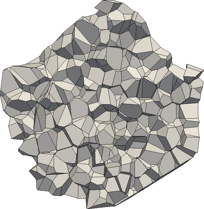
Random refers to a mesh where the control points of the Voronoi tessellation are randomly displaced inside the domain. We underline that these kind of meshes are characterized by stretched polyhedrons so the robustness of the VEM will be severely tested.
CVT refers to a Centroidal Voronoi Tessellation, i.e., a Voronoi tessellation where the control points coincides with the centroid of the cells they define. We generate such meshes via a standard Lloyd algorithm [21]. In this case the Voronoi cells are more regular than the ones of the previous case.
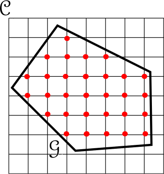
Structured refers to meshes composed by structured cubes inside the domain and arbitrary shaped mesh close to the boundary. This mesh is built by considering as control points the vertices of a structured mesh of a cube (containing the input geometry ) which are inside , see Figure 2 for a two dimensional example. When we consider the cube , this kind of mesh coincides with a structured mesh composed by cubes. These meshes are really interesting from the computational point of view. Indeed, the VEM local matrices are exactly the same for all cubes inside the domain. It is therefore possible to compute such local matrices only once so the computational effort in assembling the stiffness matrix as well as the right hand side is reduced. Moreover, the ensuring scheme may inherit some advantages of structural cubic meshes.
 |
 | |
| (a) | (b) |
| Random | ||
 |
 | |
| CVT | ||
 |
 | |
| Structured | ||
 |
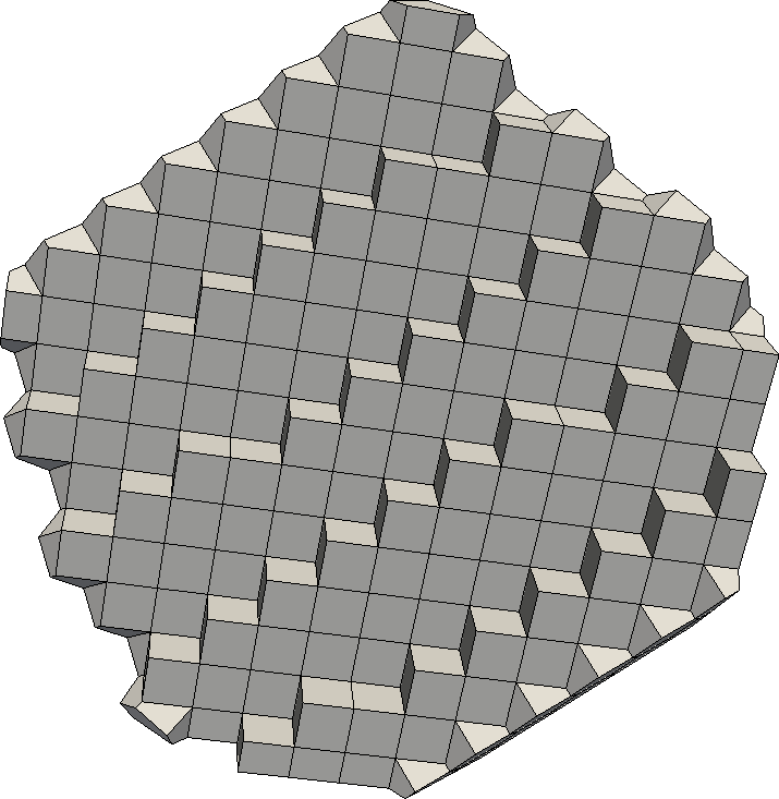 | |
In Figure 3 we collect an example on the truncated octahedron geometry of all these kinds of meshes. To analyze the error convergence rate, we make a sequence of meshes with decreasing size for each mesh type.
3.1.2 Error norms
Let be the exact solution of the PDE and the discrete solution provided by the VEM. To evaluate how this discrete solution is close to the exact one, we use the local projectors of degree on each polyhedron of the mesh, and , defined in (13) and (14), respectively. We compute the following quantities:
- •
-seminorm error
- •
-norm error
- •
-norm error
where is the set of all the vertexes and internal edge nodes of the VEM scheme, see Equations (15) and (16). Since we do not take the over all the domain but only on some nodes, is an approximation of the true -norm. Moreover, in this case we can directly compute such quantity without resorting to the projections operators.
In the following subsections we will present some numerical tests to underline different computational aspects of the method. In all cases the mesh-size parameter is measured in an averaged sense
| (24) |
with denoting the number of polyhedrons in the mesh.
3.2 Test case 1: -analysis for diffusion problem on a cube
Let us consider the problem
| (25) |
where the domain is the cube and is the union of the four faces corresponding to the planes , , and . We choose the right hand side and in such a way that the exact solution is
In this example we consider all the three types of discretizations introduced in Subsection 3.1, i.e., Random, CVT and Structured. Note that in this case the last type of discretization becomes a standard structured cubic mesh.
In Figure 4 we show the resulting graphs and in Tables 1 and 2 we provide the convergence rates. These data show that we achieve the theoretical convergence rate for all the VEM approximation degrees and for each type of meshes, see equations (22), (23).
| convergence rates | |||
|---|---|---|---|
| mesh type | |||
| Structured | 1.0344 | 2.0543 | 3.0125 |
| Random | 1.0927 | 2.0465 | 3.0656 |
| CVT | 1.0492 | 2.0672 | 3.0970 |
| convergence rates | |||
|---|---|---|---|
| mesh type | |||
| Structured | 1.9763 | 3.2551 | 4.0372 |
| Random | 1.9136 | 3.1067 | 4.0678 |
| CVT | 2.0230 | 3.2144 | 4.4620 |
 |
 |
 |
 |
 |
 |
3.3 Test case 2: -analysis for diffusion-reaction problem on a polyhedron
In this example we consider the problem
| (26) |
where the domain is the truncated octahedron, see Figure 1 (b), and we choose the right hand side and in such a way that the exact solution is
In this example we analyze the convergence rate for VEM approximation degrees from 1 to 3, and compare the results obtained with the three mesh types described in Subsection 3.1.1.
In Figure 5 we plot the convergence graphs with respect to the total number of degrees of freedom . Considering that (for fixed order and for fixed mesh family) the mesh-size parameter is expected to behave as it follows that both error norms behave as expected from the theory (see (22) and (23)).
Moreover we observe that the error is slightly affected by the shape of the mesh elements. Indeed, the errors associated with the Random mesh are always larger than the ones obtained with a more regular mesh, while the Structured meshes yield the best results (even when compared to the CVT meshes).
 |
 |
 |
 |
 |
 |
3.4 Test case 3: convergence analysis with different
In this example we consider the convergence with respect to the accuracy degree . We fix the truncated octahedron geometry and we solve the following problem
| (27) |
where the right hand side and the boundary condition are chosen in such a way that the exact solution is
The mesh is kept fixed (the CVT mesh of the truncated octahedron composed by 116 polyhedrons) and we rise the polynomial degree from 1 to 5. In Figure 6 we provide the convergence graphs of both -seminorm and -norm. The trend of these errors show an exponential convergence in terms of and are thus aligned with the existing theory for the two-dimensional case [22]. However, both the and the errors show a slight bend in the convergence graphs for . This behavior is probably due to the stabilizing matrix (19) that should be better devised in order to develop a spectral approximation strategy.
 |
 |
Although such aspect deserves a deeper study, that is beyond the scopes of the current paper, we propose a novel stabilization strategy which, at least in the present context, cures the problem.
Let represents the canonical basis functions on element , defined by
where we refer to (19) for the notation. Then, a diagonal stabilization form should satisfy (see (20) and [1, 2])
in order to mimic the original energy of the basis functions. The original form in (19) corresponds to assuming , that (considering the involved scalings) can be shown to be a reasonable choice with respect to (and thus for moderate ). On the other hand, choice (19) may be less suitable for a higher , especially in three dimensions, where different basis functions may carry very different energies. We therefore propose a simple alternative (still using a diagonal stabilizing form)
Note that at the practical level computing is immediate, since such term is simply the term on the diagonal of the consistency matrix , that is already computed.
The choice above, referred in the following as diagonal recipe, cures the problem, see Figure 7. This fact is further confirmed by the data in Table 3. Here, we compute the slopes of these lines at each step and we numerically show that the recipe diagonal stabilization yields better results.
 |
 |
| convergence | ||||
|---|---|---|---|---|
| 2-5 Original | -1.3219 | -1.4065 | -1.3045 | -0.6195 |
| Recipe | -1.3218 | -1.4144 | -1.9211 | -1.8977 |
| convergence | ||||
| Original | -1.5704 | -1.6532 | -1.5736 | -1.1455 |
| Recipe | -1.5698 | -1.6850 | -1.4805 | -2.3065 |
3.5 Test case 4: patch test
In [1, 2] it is shown that VEM passes the so-called “patch test”. If we are dealing with a PDE whose solution is a polynomial of degree and we use a VEM approximation degree equal to , we recover the “exact solution”, i.e., the solution up to the machine precision.
We make a patch test for VEM approximation degrees from 1 up to 5. More specifically, we consider the following PDE
| (28) |
where the right hand side and the Dirichlet boundary condition are chosen in accordance with the exact solution
Since we are not interested in varying the mesh size but only the VEM approximation degree, we run the experiments on the same coarse CVT mesh of the truncated octahedron composed by 116 polyhedrons.
In Table 4 we collect the results. The errors are close to the machine precision, but for higher VEM approximation degrees they become larger. This fact is natural and stems from the conditioning of the matrices involved in the computation of the VEM solution. Indeed, as in standard FEM, their condition numbers become larger when we consider higher VEM approximation degrees.
| solution degree | -seminorm | -seminorm | -norm |
|---|---|---|---|
| 1 | 5.9775e-12 | 6.1919e-13 | 1.1479e-12 |
| 2 | 2.2008e-11 | 1.8416e-12 | 4.9409e-12 |
| 3 | 1.0490e-10 | 1.1284e-11 | 8.5904e-12 |
| 4 | 3.0959e-10 | 1.0039e-10 | 2.6197e-11 |
| 5 | 1.1563e-09 | 6.9693e-09 | 1.5433e-10 |
3.6 Test case 5: stabilizing parameter analysis
In this example we make an analysis on the stabilizing part of the local stiffness matrix. We slightly modify defined in Subsection 2.5 by introducing the parameter , i.e.,
| (29) |
We fix a standard Poisson problem
| (30) |
where and whose exact solution is
We exploit the same discretization of , a CVT mesh composed by 1024 polyhedrons, and solve this problem for many values of the parameter . More specifically, we consider for one hundred uniformly distributed values of in and we compute the errors for the corresponding VEM solutions in the -seminorm and -norm.
 |
 |
| (a) | (b) |
In Figure 8 we provide the graphs of both errors, as a function of in a logarithmic scale, for VEM approximation degree and . We can observe that the trend of the errors is the same for each : it grows whenever very small or very large choices are taken for the parameter. Although the -norm seems more sensible than the -seminorm, the method appears in general quite robust with respect to the parameter choice. For instance, we show in Table 5 the quantities
representing the ratios of maximum to minimum error for the parameter range , that corresponds to a factor of 100 between minimum and maximum . From this table we can appreciate that the error ratios are all within an acceptable range.
| 1 | 1.4487e+00 | 8.9624e+00 |
|---|---|---|
| 2 | 1.7014e+00 | 4.9538e+00 |
| 3 | 1.3884e+00 | 2.0908e+00 |
| 4 | 2.6989e+00 | 4.8393e+00 |
Aknowledgments
The first and second authors have received funding from the European Research Council (ERC) under the European Unions Horizon 2020 research and innovation programme (grant agreement no. 681162).
References
- [1] L. Beirão da Veiga, F. Brezzi, A. Cangiani, G. Manzini, L. D. Marini, A. Russo, Basic principles of Virtual Element Methods, Math. Models Methods Appl. Sci. 23 (2013) 119–214.
- [2] L. Beirão da Veiga, F. Brezzi, L. D. Marini, A. Russo, The hitchhikers guide to the virtual element method, Math. Models Methods Appl. Sci. 24 (8) (2014) 1541–1573.
- [3] L. Beirão da Veiga, C. Lovadina, G. Vacca, Divergence free virtual elements for the stokes problem on polygonal meshes, ESAIM Math. Model. Numer. Anal. 51 (2) (2017) 509–535.
- [4] F. Brezzi, L. Marini, Virtual Element Method for plate bending problems, Comput. Methods Appl. Mech. Engrg. 253 (2012) 455–462.
- [5] P. Antonietti, L. Beirão da Veiga, S. Scacchi, M. Verani, A virtual element method for the Cahn-Hilliard equation with polygonal meshes, SIAM Journal on Numerical Analysis 54 (1) (2016) 34–56.
- [6] B. Ahmed, A. Alsaedi, F. Brezzi, L. Marini, A. Russo, Equivalent Projectors for Virtual Element Methods, Comput. Math. Appl. 66 (3) (2013) 376–391.
- [7] L. Beirão da Veiga, F. Brezzi, L. D. Marini, A. Russo, Virtual element methods for general second order elliptic problems on polygonal meshes, Math. Models Methods Appl. Sci. 26 (4) (2016) 729–750.
- [8] H. Chi, L. Beirao da Veiga, G. Paulino, Some basic formulation of the virtual element method (VEM) for finite deformations, Comput. Meth. Appl. Mech. Engrg. 318 (09) (2017) 148–192.
- [9] B. Ayuso, K. Lipnikov, G. Manzini, The nonconforming virtual element method, ESAIM: M2AN 50 (3) (2016) 879–904.
- [10] M. F. Benedetto, S. Berrone, A. Borio, S. Pieraccini, S. Scialò, A hybrid mortar virtual element method for discrete fracture network simulations, Journal of Computational Physics 306 (2016) 148 – 166.
- [11] E. Caceres, G. Gatica, A mixed virtual element method for the pseudostress–velocity formulation of the stokes problem, IMA J. of Numer. Anal. 37 (1) (2017) 296–331.
- [12] D. Mora, G. Rivera, R. Rodríguez, A virtual element method for the Steklov eigenvalue problem, Math. Models Methods Appl. Sci. 25 (8) (2015) 1421–1445.
- [13] A. Gain, G. Paulino, S. Leonardo, I. Menezes, Topology optimization using polytopes, Comput. Methods Appl. Mech. Engrg. 293 (2015) 411–430.
- [14] G. Vacca, Virtual element methods for hyperbolic problems on polygonal meshes, Comput. Math. Appl.doi:http://dx.doi.org/10.1016/j.camwa.2016.04.029.
- [15] L. Beirão da Veiga, A. Chernov, L. Mascotto, A. Russo, Exponential convergence of the hp virtual element method with corner singularities (2016). arXiv:1611.10165.
- [16] A. Gain, C. Talischi, G. Paulino, On the Virtual Element Method for Three-Dimensional Elasticity Problems on Arbitrary Polyhedral Meshes, Comp. Meth. in Appl. Mech. and Engrng. 282 (2014) 132 – 160.
- [17] A. Cangiani, E. Georgoulis, T. Pryer, O. Sutton, A posteriori error estimates for the virtual element method, Preprint arXiv:1603.05855.
- [18] L. Beirao da Veiga, C. Lovadina, A. Russo, Stability analysis for the virtual element method, Preprint arXiv:1607.05988.
- [19] R. Williams, The Geometrical Foundation of Natural Structure: A Source Book of Design, Dover Publications, 1979.
- [20] C. H. Rycroft, Voro++: A three-dimensional voronoi cell library in c++, Chaos 19 (4) (2009) 041111.
- [21] Q. Du, V. Faber, M. Gunzburger, Centroidal voronoi tessellations: Applications and algorithms, SIAM Rev. 41 (4) (1999) 637–676.
- [22] L. Mascotto, L. Beirao da Veiga, A. Chernov, A. Russo, Basic principles of hp virtual elements on quasiuniform meshes, Math. Mod. and Meth. in Appl. Sci. 26 (08) (2016) 1567–1598.