A multigrid algorithm for the –version of the Virtual Element Method Thanks: Paola F. Antonietti has been partially supported by the Fondazione Cariplo and Regione Lombardia research grant n. 2015-0182: “PolyNum: Polyhedral numerical methods for partial differential equations”. M. Verani has been partially supported by the Italian research grant Prin 2012 2012HBLYE4 “Metodologie innovative nella modellistica differenziale numerica” and by INdAM-GNCS
Abstract
We present a multigrid algorithm for the solution of the linear systems of equations stemming from the version of the Virtual Element discretization of a two-dimensional Poisson problem. The sequence of coarse spaces are constructed decreasing progressively the polynomial approximation degree of the Virtual Element space, as in standard -multigrid schemes. The construction of the interspace operators relies on auxiliary Virtual Element spaces, where it is possible to compute higher order polynomial projectors. We prove that the multigrid scheme is uniformly convergent, provided the number of smoothing steps is chosen sufficiently large. We also demonstrate that the resulting scheme provides a uniform preconditioner with respect to the number of degrees of freedom that can be employed to accelerate the convergence of classical Krylov-based iterative schemes. Numerical experiments validate the theoretical results.
Introduction
In recent years there has been a tremendous interest in developing numerical methods for the approximation of partial differential equations where the finite-dimensional space is built upon an underlying mesh composed by arbitrarily-shaped polygonal/polyhedral (polytopic, for short) elements. Examples of methods that have been proposed so far include Mimetic Finite Differences [47, 34, 48, 28], Polygonal Finite Element Methods [52, 53], Discontinuous Galerkin Finite Element Methods [6, 9, 15, 38, 37, 8, 36] Hybridizable and Hybrid High Order Methods [41, 42, 40], and Gradient schemes [45, 43], for example. Recently, in [23] the Virtual Element Method (VEM) has been introduced, and further developed for elliptic and parabolic problems in [25, 22]. VEMs for linear and nonlinear elasticity have been developed in [24, 46, 21], whereas VEMs for plate bending, Cahn-Hilliard, Stokes, and Helmholtz problems have been addressed in [35, 5, 4, 50]. For discrete topology optimization and fracture networks problems we refer to [7] and [29], respectively. Moreover, several variants of the Virtual Element Method, including mixed, and -conforming, serendipity and nonconforming VEMs have been proposed in [33, 19, 18, 20, 14, 39, 56, 11].
All the above mentioned contributions focus on the –version of the Virtual Element Method.
The -version VEM was introduced in [26] for the 2D Poisson problem, considering quasi-uniform meshes.
It was shown that, analogously to the -version Finite Element Method (FEM) case,
if the solution of the problem has fixed Sobolev regularity, then the convergence rate of the method in terms of is algebraic,
whereas if the solution is analytic then the convergence rate is exponential.
In [27], the full -version VEM was studied based on employing meshes geometrically graded towards the corners of the domain and properly choosing the
distribution of polynomial approximation degree, so that the convergence rate of the method is exponential in terms of the number of degrees of freedom.
So far, the issue of developing efficient solution techniques for the linear systems of equations stemming
from both the -, - or -versions of the VEM
has not been addressed yet. The main difficulty in the
development of optimal (multilevel) solution techniques relies on the
construction of consistent coarse solvers which are non-trivial
on grids formed by general polyhedra. Very recently, using the techniques of [12, 13]
a multigrid algorithm for the -version Discontinuous Galerkin methods
on agglomerated polygonal/polyhedral meshes has been analyzed in
[10].
The aim of this paper is to develop efficient iterative solvers for the solution of the linear systems of equations stemming from the –version of the Virtual Element discretization of a two-dimensional Poisson problem. We propose to employ a W-cycle -multigrid multigrid algorithm, i.e. coarse levels are obtained by decreasing progressively the polynomial approximation degree up to the coarsest level which corresponds to the lowest (linear) Virtual Element (VE in short) space. The key point is the construction of suitable prolongation operators between the hierarchy of VE spaces. With the standard VE space such prolongation operators cannot be constructed based on employing only the degrees of freedom. For such a reason we introduce a suitable auxiliary VE space, which is identical to the standard VE space from the algebraic point of view and which allows to construct computable interspace operators but results into non-inherited sublevel solvers. This in turn complicates the analysis of the multigrid algorithms, since we need to account for non-inherited sublevel solvers. Employing a Richardson smoother and following the classical framework, see e.g. [32], we prove that the W- cycle algorithm converges uniformly provided the number of smoothing steps is chosen sufficiently large. We also demonstrate that the resulting multigrid algorithm provides a uniform preconditioner for the Preconditioned Conjugate Gradient method (PCG), i.e., the number of PCG iterations needed to reduce the (relative) residual up to a (user-defined) tolerance is uniformly bounded independently of the number of degrees of freedom. Further, employing the Gauss-Seidel smoother in place of the Richardson one can improve the performance of our iterative scheme.
The extension of the present setting to -multigrid methods, i.e. where the coarse levels are formed by geometric agglomeration of the underlying grid is currently under investigation.
The remaining part of the paper is organized as follows. In Section 1, we introduce the model problem, a Virtual Element Method approximating its solution, the associated linear system and the multigrid algorithm;
moreover, an auxiliary VE space, needed for the construction of the algorithm, is presented.
In Section 2, we present the -cycle VEM multigrid algorithm; its convergence analysis is the topic of Section 3.
Finally, in Section 4, numerical results are shown.
Throughout the paper, we will adopt the standard notation for Sobolev spaces (see [44, 2]). In particular, given , and are the standard Lebesgue and Sobolev spaces over , respectively, and , , and , are the Lebesgue and the Sobolev (semi)norms, respectively. We will write and meaning that there exist positive constants , and independent of the discretization and multigrid parameters, such that and , respectively. In addiction, , , , denotes the space of polynomials of maximum degree over , with the the convention . We will also employ the standard multi-index notation:
| (1) |
1 The model problem and the -version Virtual Element Method
Let be a polygonal domain and we consider the following model problem: find :
| (2) |
. Problem (2) is well-posed, cf. [32], for example. In the next section we introduce the -version of the Virtual Element Method and we discuss its implementation. In Section 1.2, we build an auxiliary VE space that will be instrumental to construct and analyse our multigrid algorithm.
1.1 The -version Virtual Element Method
In this section, we introduce the –version Virtual Element Method, based on polygonal meshes with straight edges for the discretization of problem (2).
Let be a fixed decomposition of into non-overlapping polygonal elements , and let and be the set of all vertices and edges of , respectively. We set and .
Given generic polygon in , we also define and as the set of vertices and edges of polygon , respectively.
To each edge , we associate and , the tangential and normal unit vector (obtained by a counter-clockwise rotation of ), respectively.
For future use, it is convenient to split the (continuous) bilinear form defined in (2) into a sum of local contributions:
In order to construct the -VEM approximation of (2), we need the following ingredients:
- •
Finite dimensional subspaces of and a finite dimensional subspace of , such that ;
- •
Local symmetric bilinear forms so that:
(3) - •
A duality pairing , where and is the dual space of .
The above ingredients must be built in such a way that the discrete version of (2):
| (4) |
is well-posed and optimal a priori energy error estimates hold, cf. [26].
We begin by introducing the local space ; given and , we set:
| (5) |
where
| (6) |
We remark that the above definition coincides with the definition of the two dimensional VE space introduced in [23] for the Poisson equation, and that clearly , . The global space is then obtained by gluing continuously the local spaces:
| (7) |
We note that for the sake of simplicity we are assuming a uniform on each . Nevertheless, it is possible to construct VEM with non-uniform degrees of accuracy over , see [27].
We endow the space (5) with the following set of degrees of freedom (dofs). To every we associate:
- •
the values of at the vertices of ;
- •
the values of at distinct internal nodes on each edge ;
- •
the scaled internal moments:
(8) where is an orthonormal basis of .
Reasoning as in [23, Proposition 4.1], it is easy to see that this is a unisolvent set of degrees of freedom. We observe that the basis introduced in (8) can be built by orthonormalizing (following, e.g., [16]) for instance the monomial basis given by:
| (9) |
where denotes the barycenter of the element .
Remark 1.
The definition of the internal degrees of freedom in (8) differs from its classical counterpart in [23, 26] where the internal moments are defined with respect to the monomial basis (9). The new choice of the internal degrees of freedom will play a crucial role in the choice of the stabilization of the method, see Theorem 1.1, and in the choice of the space-dependent inner product associated with the multigrid algorithm, see Theorem 2.1 below.
We define the canonical basis as:
| (10) |
Owing the definition (5) of the local VE space and the choice of the degrees of freedom, it is possible to compute the following operators:
- •
the projection operator :
(11) - •
the projector :
(12)
see [23, 17] for details.
We observe that the last two conditions in (12) are needed in order to fix the constant part of the energy projector.
Next, we introduce the discrete right-hand side and the associated duality pairing:
| (13) |
where
We observe that it is possible to compute up to machine precision the expression in (13),
because the action of the projector on all the elements of is computable.
For a deeper study concerning the approximation of the discrete loading term see [3, 24, 26].
Finally, we turn our attention to the local and global discrete bilinear forms. We require that the local bilinear forms satisfy, for all , the two following assumptions.
- (A1)
consistency:
(14) - (A2)
stability: there exist two positive constants , possibly depending on , such that:
(15)
Assumption (A1) guarantees that the method is exact whenever the solution of (2) is a polynomial of degree , whereas assumption (A2) guarantees the well-posedness of problem (4). Let now be the identity operator on the space , we set:
| (16) |
where is defined in (12) and the local bilinear form as:
| (17) |
satisfies:
| (18) |
where and might depend on . We underline that the local discrete bilinear form (16) satisfies (A1) and (A2) and, thanks to (18), the following bounds hold:
with:
| (19) |
The following result provides bounds in terms of for the constants and in (18).
Theorem 1.1.
An immediate consequence of Theorem 1.1 and (19) is that it holds:
| (20) |
where and are given in (15).
Lemma 1.2.
Let be the local auxiliary stabilization defined as:
| (21) |
Then, it holds:
| (22) |
where , , and where is the energy projector defined in (12).
Proof.
The thesis follows based on employing integration by parts, the properties of orthogonal projections and polynomial inverse estimates. It follows the lines of the proof of [27, Theorem 4.1]; for the sake of brevity the details are not reported here. ∎
Before showing the proof, we recall that given and the Gauß-Lobatto nodes and weights on , respectively, it holds:
| (23) |
cf. [30, (2.14)]. Moreover, it holds:
| (24) |
where the hidden constants are positive and independent of , see [1, (25.4.32)].
Proof.
By using (23) and (24), we obtain:
| (25) |
where denotes the -th boundary degree of freedom. This concludes the discussion concerning the boundary term. Next, we study the bulk term in (21), and consider the expansion of into the orthonormal basis introduced in (8):
| (26) |
Testing (26) with , , we obtain:
where denotes the internal degrees of freedom associated with polynomial . As a consequence:
| (27) |
Parceval identity implies:
| (28) |
where denotes the internal degree of freedom associated with polynomial . The thesis follows from (25) and (28). ∎
Remark 2.
Finally, from [23, 26] the following error bound in the energy norm holds:
| (29) |
where and are the solution of (2) and (4), respectively, and are the stability constants given in (15) and is the smallest constant satisfying:
From (29) and following [26], it is possible to prove error bounds analogous to those in the -FEM case, see [51].
Finally, we focus on the construction of the linear system of equations stemming from (4). By expanding the trial function as a combination of the elements in the canonical basis, see (10),
where is the set of dofs of , and selecting as , , we obtain:
| (30) |
where:
| (31) |
Both the right-hand side and the coefficient matrix are computable exactly up to machine precision, see [17]. In the next section, we discuss the spectral condition number of the stiffness matrix .
1.1.1 The condition number of the stiffness matrix
In (8) we defined the internal degrees of freedom associated with space defined in (5) as the scaled moments with respect to an orthonormal basis of . We observe that this choice is different from the usual choice adopted in standard VEM literature, see e.g. [23, 17, 3], where the internal dofs are defined as the (scaled) moments with respect to the monomial basis (9) of . Our choice, which is a key ingredient in the proof of Lemma 1.3. also plays a fundamental role in the spectral properties of the stiffness matrix defined in (31). Indeed, in Table 1 we compare the spectral condition number of the stiffness matrix as a function of the degree of accuracy of the method , based on employing the two different sets of internal degrees of freedom, namely the scaled moments with respect to the orthonormal basis of or with respect to the monomial basis (9). Results reported in Table 1 have been obtained on the Voronoi-Lloyd polygonal mesh shown in Figure 1; the same kind of results have been obtained on meshes made of squares and of quasi-regular hexagons. For the sake of brevity these results have been omitted. From the results reported in Table 1 it is clear that grows, as for classical finite element methods, as whenever the interior dofs are defined with respect to an orthonormal basis of whereas the condition number blows up exponentially if the scaled moments are defined with respect to the monomial basis (9). That is, the choice (8) for the internal degrees of freedom is the right choice as it damps the condition number of the stiffness matrix effectively and prevents round off errors, as those observed, for example, in [26] where the monomial basis (9) was employed.
| 1.3225e+01 | 7.2732e+01 | |
| 4.9712e+02 | 1.0964e+03 | |
| 7.5099e+02 | 1.2910e+05 | |
| 1.1823e+03 | 1.5566e+07 | |
| 1.9395e+03 | 1.6003e+09 | |
| 3.5100e+03 | 1.7069e+11 | |
| 6.0754e+03 | 1.7280e+13 | |
| 1.0100e+04 | 1.7172e+15 | |
| Rate | , , |
1.2 An auxiliary Virtual Element Space
In this section, we introduce an auxiliary VE space which will be crucial for the construction of the multigrid algorithm in Section 2. Hence, following the spirit of [3], we consider a modification of into a diverse space on which we are able to compute a higher order projector. In particular, we set:
| (32) |
where we recall that is a multi-index.
Henceforth, we will denote by the expression enhancing constraints the following set of constraints employed in the definition of :
| (33) |
The definition of is different from the one presented in [3]. Moreover, we observe that , but . To be more precise, owing to the orthonormality of the , it holds in fact:
where denotes the space of polynomials of degree , not in the space of polynomials of degree , orthogonal to all with .
We endow with the same degrees of freedom of the space introduced in (5). Using the auxiliary local virtual space introduced in (32), it is clear that we are able to compute the following operator:
- •
, the projection onto the space of polynomials of degree , defined as in (11).
We stress that there is no chance to be able to compute explicitly as a map defined on , since the internal degrees of freedom are up to order , whereas this is possible in the new space we can do that since (33) allows to compute internal moments up to order .
The global auxiliary VE space is obtained again by gluing continuously the local spaces as done in (7):
| (34) |
The choice of the discrete bilinear form and of the right-hand side in (4) are exactly the same as those in Section 1.1 for the space .
It is crucial to remark that the linear systems stemming from the use of and are the same. In fact, it is clear from (16) that the construction of the local discrete bilinear forms depends uniquely on the choice of the set of the degrees of freedom (which we recall are the same for the two spaces) and the energy projector defined in (12), which is computed without the need of (33).
Also the construction of the discrete right-hand side (13) does not depend on the choice of the space since the projector defined in (11) is built using the internal degrees of freedom only, while the enhancing constraints (33) are neglected.
Remark 3.
The aforementioned equivalence between the two linear systems associated with spaces and is of great importance in order to design and analyse the multigrid algorithm in Section 2. However, and have significant differences.
The first issue we want to highlight is that the method associated with space (34) is not a “good” method from the point of view of the approximation property. It is possible to show approximation results on the first and the third term on the right hand side of (29) following for instance [26, Sections 4 and 5]. The problematic term is the second one, i.e. the best error term with respect to functions in the virtual space. The approach used in [26], which is the –version of [49, Proposition 4.2], does not hold anymore in the enhanced version of VEM. At the best of the authors knowledge, the approximation of the “best virtual” error term in enhanced space is still an open problem. On the other hand, the error analysis with space is available in [26].
Let us summarize the strategy we will follow. We consider a discretization of (2) by means of the Virtual Element Method (4) employing as an approximation space defined in (7). The associated linear system (30) coincides algebraically with the one arising by employing the VE space defined in (34). For this reason, we can solve system (30) by means of a multigrid algorithm based on the sequences of spaces defined in (34).
2 Multigrid algorithm with non-inherited sublevel solvers
In this section, we present a -VEM multigrid algorithm and the key ingredients for its formulation.
In the construction of our multigrid algorithm, we will make use of two key ingredients. The first one are suitable (computable) interspace operators, i.e. prolongation/restriction operators between two VE spaces. These operators will be constructed by employing the properties of the following space-dependent inner product:
| (35) |
The second ingredient is a suitable smoothing scheme , which aims at reducing the high frequency components of the error.
We aim at introducing a multigrid iterative method for the solution of the linear system in (30), which we recall is given by:
| (36) |
where the coefficient matrix and the right-hand side are the matrix representations with respect to the their expansion in the canonical basis of space , defined in (34), of the operators:
| (37) |
In order to introduce our -multigrid method, we consider a sequence of VE spaces given by , where the -th level is given by , . Let now consider the linear system of equations on level : . We denote by one iteration obtained by applying the -th level iteration of our MG scheme to the above linear system, with initial guess and using post-smoothing steps, respectively. For , (coarsest level) the solution is computed with a direct method, that is while for we adopt the recursive procedure described in Algorithm 1.
In presenting Algorithm 1, we used some objects that are not defined so far. In particular, denotes the matrix representation of the interspace operators defined in Section 2.2, while denotes the matrix representation of the smoothing operator defined in Section 2.3.
For a given, user defined tolerance tol and a given initial guess , the full -multigrid algorithm employed to solve (36) is summarized in Algorithm 2; its analysis is presented in the forthcoming Section 3.
Remark 4.
As a byproduct, we underline that it is possible to employ multigrid algorithms where two “adjacent” levels, associated to spaces and , respectively, satisfy . In such cases, to build the interspace operators, it suffices to modify the definition (32) by using a “larger” enhancing technique and imposing that the laplacian of functions in the virtual space is a polynomial of higher degree, and then reduce the space with additional constraints on the -projectors.
2.1 Space-dependent inner products
The aim of this section is to prove the following result on the space-dependent inner product (35), which will be useful for the forthcoming analysis.
Theorem 2.1.
In order to prove Theorem 2.1, it suffices to combine the forthcoming technical results. The first one makes use of the following auxiliary space-dependent inner product defined as:
| (39) |
where the local contributions read:
| (40) |
Lemma 2.2.
Before showing the proof, we recall that from [27, Theorem 7.5] the following inverse-type holds holds:
| (42) |
where:
| (43) |
Proof.
(Proof of Lemma 2.2) The proof is slightly different from the one for the stability bounds (22); in fact, here we work on the complete virtual space and not on , being defined in (12). In the following, we neglect the dependence on the size of the elements since we are assuming that the mesh is fixed; the general case follows from a scaling argument. The upper bound follows from a trace inequality and the stability of orthogonal projection
and summing up on all the mesh elements and applying the Poincarè inequality. For the lower bound, by using an integration by parts and the definition of the local auxiliary space (32), we have:
| (44) |
Owing to (42) and recalling that , we deduce:
| (45) |
We bound now the two terms appearing on the right-hand side of (44). Applying (45), we have:
| (46) |
Applying next a Neumann trace inequality [51, Theorem A.33], a one dimensional inverse inequality, the interpolation estimates [55, 54] and (45), we get:
| (47) |
Substituting (46) and (47) in (44), we obtain:
whence
The thesis follows summing on all the elements. ∎
Proof.
The proof is a straightforward modification of the one of Lemma 1.3. ∎
Remark 5.
The choice (35) for the space-dependent inner product is crucial for the construction of the interspace operators, see Section 2.2. Moreover, we point out that it coincides with the usual choice for the space-dependent inner product in the DG-Finite Element Framework, see [12, 10]. The Finite Element counterpart of Theorem 2.1 is much less technical, since it suffices to choose an orthonormal basis of polynomials as canonical basis; via Parceval identity, the (scaled) norm is spectrally equivalent to the space-dependent inner product (35); thus, the employment of polynomial inverse inequality implies a straightforward relation with the seminorm. In the VEM framework, it is not possible to proceed similarly for two reasons. The first one is that, at the best of the authors knowledge, inverse inequalities for functions in virtual spaces are not available; the second reason is that an orthonormal basis of functions in the virtual space is not computable, since such functions are not known explicitly.
2.2 Interspace operators
In this section, we introduce and construct suitable prolongation and restriction operators acting between the VE spaces and , . First of all, we stress that the sequence of local spaces , and thus the associated sequence of global spaces , are not nested. As a consequence, we cannot define the prolongation interspace operator simply as the natural injection, as done for instance in [32, 31, 12, 10]. In our context, the prolongation operator:
| (49) |
associates to a function in a function in , having the same values as for all the dofs that are in common with space , while the remaining values of the dofs (i.e. the internal higher order ones) are computed using the enhancing constraints presented in definition (32). More precisely, we define as:
| (50) |
since are the elements of an -orthonormal basis of . We recall that the third equation in (50) follows from the enhancing constraints in the definition of local spaces (32). The restriction operator is defined as the adjoint of with respect to the space-dependent inner product defined in (35), i.e.:
| (51) |
We remark that, thanks to definition (35) of the space-dependent inner product, the matrix associated with is the transpose of the matrix associated with the operator .
2.3 Smoothing scheme and spectral bounds
In this section, we introduce and discuss the smoothing scheme entering in the multigrid algorithm. To this aim, we introduce the following space-dependent norms:
| (52) |
We highlight that it holds:
Since the matrix is a symmetric positive definite matrix, there exists an orthonormal (with respect to the inner product ) basis of eigenvectors of , and the associated eigenvalues are real and strictly positive. Let be the related set of eigenpairs. We show now a bound of the spectrum of in terms of .
Lemma 2.4.
Proof.
As a smoothing scheme, we choose a Richardson scheme, which is given by:
| (54) |
where . A numerical study concerning the (sharp) dependence of on of the spectral bound is presented in Section 4.
2.4 Error propagator operator
As in the classical analysis of the multigrid algorithms [32], in this section we introduce and analyze the error propagator operator. To this aim, we firstly consider a “projection” operator , defined as the adjoint of with respect to inner product , i.e.:
| (55) |
The following auxiliary result holds.
Lemma 2.5.
Proof.
As the proof is very similar to its analogous version in [32, Lemma 6.4.2], here we briefly sketch it. For all :
∎
We now introduce the error propagator operator:
| (57) |
where the relaxation operator is defined as:
| (58) |
The following result holds.
Theorem 2.6.
3 Convergence analysis of the multigrid algorithm
We prove in Section 3.5 the convergence of the multigrid algorithm presented in Section 2. For the purpose, we preliminarily introduce some technical tools. In Section 3.1, we discuss the so-called smoothing property associated with the Richardson scheme (54). In Section 3.2, we show bounds related to the prolongation operator (49) and its adjoint with respect to the space-dependent inner product (35). Bounds concerning the error correction steps are the topic of Section 3.3. Finally, in Sections 3.4 and 3.5, we treat the convergence of the two-level and multilevel algorithm, respectively.
3.1 Smoothing property
Lemma 3.1.
Proof.
The proof is analogous to that in [12, Lemma 4.3]. For the sake of clarity, we report the details. To start with, we rewrite in terms of the orthonormal basis of eigenvectors of as follows:
As a consequence,
where is the upper bound for the spectrum of presented in Lemma 2.4. Then, owing to the orthonormality of with respect to the inner product , we have:
where in the last inequality we used [12, Lemma 4.2] and (53). ∎
3.2 Prolongation and projection operators
In this section, we prove bounds in the norm of the prolongation and the projection operators defined in (49) and (55), respectively. We stress that this set of results deeply relies on the new enhancing stategy presented in the definition of the virtual space (32).
We start with a bound on the prolongation operator.
Theorem 3.2.
Proof.
Recalling bounds (15), (41) and the definition of the auxiliary space-dependent inner product (39), we have:
| (64) |
We recall that:
Since defined in (6) is a sequence of nested space for all , we directly have:
where denotes the -th boundary dof.
Now, we deal with the internal degrees of freedom. We cannot use the above nestedness argument since the sequence is made of non-nested spaces. In order to overcome this hindrance, recalling the definition of the prolongation operator (50), we write:
where denotes the -th internal dof. As a consequence, it holds:
| (65) |
Next, we relate with . We note that:
| (66) |
where we used in the last but one and in the last inequalities (38) and (15), respectively.
We show an analogous bound for the “projection” operator introduced in (55).
Theorem 3.3.
Proof.
3.3 Error correction step
In this section, we prove a bound for the error correction step discussed in the multigrid algorithm, see Table .
Theorem 3.4.
3.4 Convergence of the two-level algorithm
In this section, we prove the convergence of the two-level algorithm.
Theorem 3.5.
As a consequence of Theorem 3.5, we deduce that taking , number of postsmoothing iterations large enough, the two-level algorithm converges, since the two-level error propagator operator is a contraction. We point out that a sufficient condition for the convergence of the two-level algorithm is that the number of postsmoothing iterations must satisfy:
| (70) |
see Remark 6 for more details. We stress that (70) is a sufficient condition only, in practice the number of postsmoothing steps needed for the convergence of the algorithm is much smaller; see numerical results in Section 4.
3.5 Convergence of the multilevel algorithm
In this section, we prove the main result of the paper, namely the convergence of our -VEM multigrid algorithm.
Theorem 3.6.
Let and be defined as in Theorem 3.5. Let be defined as in Theorem 3.3. Let and be defined in (15) and and be defined in (41). Then, there exists such that, if the number of postsmoothing iterations satisfies:
| (71) |
then, it holds:
with . As a consequence, this implies that the multilevel algorithm converges uniformly with respect to the discretization parameters and the number of levels provided that satisfies (71), since is a contraction.
Proof.
From Theorem 3.5, we have that:
Recalling (57), we decompose the error propagator operator as:
Thus:
We bound the two terms separately. The first one is estimated directly applying the two-level error result, namely Theorem 3.5:
On the other hand, the second term can be bounded applying the smoothing property Lemma (3.1), the bounds regarding the interspace operator Theorem 3.2, the induction hypothesis and Theorem 3.3. We can write:
We note that owing to (20) and (38), the following holds true:
We deduce:
We want that is such that . In particular, we require:
which is in fact equivalent to (71). ∎
Remark 6.
We briefly comment on equations (70) and (71) highlighting the origin of the different terms:
- *
- *
the term is related to (38) which is not robust; again, if it were possible to provide space-dependent inner products spectrally equivalent to the seminorm, then .
The existence of a independent stabilization of the method and the existence of a computable virtual -orthonormal basis is still, at the best of the authors knowledge, an open issue.
4 Numerical results
In this section, we test the performance of the multigrid solver for the -version of the VEM by studying the behaviour of the convergence factor:
| (72) |
where denotes the iteration counts needed to reduce the residual below a given tolerance of and , are the final and the initial residuals, respectively. We also show that our multigrid algorithm can be employed as a preconditioner for the PCG method. Throughout the section we fix the maximum number of iterations to and consider three different kind of decompositions: meshes made of squares, Voronoi-Lloyd polygons and quasi-regular hexagons; cf. Figure 1.


In Section 4.1, we present some tests aiming at assessing the performance of our multigrid scheme with different smoothers. In Section 4.2 we show that our multigrid method can be successfully employed as a preconditioner for the Congiugate Gradient (CG) iterative scheme, more precisely we consider a single iteration of the multigrid algorithm as a preconditioner to accelerate the Preconditioned CG method.
4.1 The –multigrid algorithm as an iterative solver
In this section we investigate the performance of our multigrid scheme with different smoothers. We consider both the Richardson scheme (54) as well as a symmetrized Gauß-Seidel scheme as a smoother.
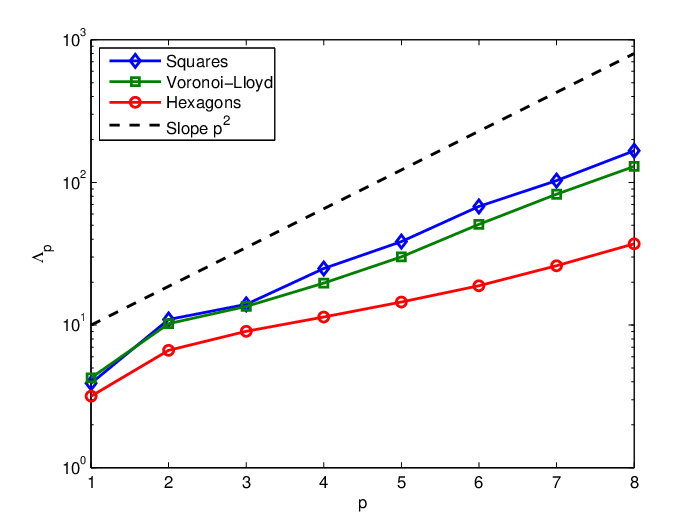
The first set of numerical experiment has been obtained based on employing a Richardson smoother. Before presenting the computed estimates of the convergence factor, we investigate numerically the behaviour of the smoothing parameter associated with the Richardson scheme (54), for which a far-from-being-sharp bound is given in Lemma 2.4. As shown in Figure 2, where as a function of is shown, the maximum eigenvalue of seems to behave even better than , which is the expected behaviour in standard Finite Elements. The numerical tests presented in the following have been obtained with an approximation of obtained (in a off line stage) with ten iterations of the power method.
In this section, we numerically investigate the behaviour of the multigrid algorithm using a Richardson smoother. The results reported in Table 2 shows the computed convergence factor defined in (72) as a function of the number of level , the number of postsmoothing steps , and the degree of accuracy employed at the “finest level” on a mesh made of squares, cf. Figure 1. Analogous results have been obtained on the other decompositions; such results are not reported here for the sake of brevity. As expected, increasing the number of postsmoothing implies a decreasing of the convergence factor . Moreover, a minimum number of smoothing steps is required to guarantee the convergence of the underlying solver. We also observe that, as expected, even though both two-level and multilevel solvers converge for a fixed value of , the number of iterations required to reduce the relative residual below the given tolerance grows with increasing .
| K | 2 | 2 | 3 | 3 | 4 | 3 | 4 |
|---|---|---|---|---|---|---|---|
| 0.99 | x | 0.97 | x | 0.97 | x | x | |
| 0.97 | x | 0.95 | x | 0.92 | x | x | |
| 0.96 | 0.93 | 0.92 | 0.79 | 0.88 | x | 0.85 | |
| 0.95 | 0.69 | 0.89 | 0.74 | 0.84 | 0.98 | 0.82 | |
A numerical estimate of the minimum number of postsmoothing steps needed in practice to achieve convergence is reported in Table 3 for all the meshes depicted in Figure 1. This represents a practical indication for (71) As expected, such a minimum number depends on the polynomial degree employed in the finest level.
| K | 2 | 2 | 3 | 2 | 3 | 4 | 2 | 3 | 4 | 2 | 3 | 4 |
|---|---|---|---|---|---|---|---|---|---|---|---|---|
| Square | 1 | 6 | 1 | 10 | 5 | 1 | 14 | 8 | 5 | 42 | 15 | 8 |
| Voronoi-Lloyd | 7 | 14 | 5 | 12 | 11 | 5 | 14 | 10 | 11 | 36 | 24 | 9 |
| Hexagons | 7 | 25 | 6 | 12 | 20 | 5 | 9 | 10 | 19 | 17 | 7 | 9 |
We next investigate the behaviour of our MG algorithm whenever a symmetrized Gauß-Seidel scheme as a smoother is employed. We recall that the smoothing matrix associated with the symmetrized Gauß-Seidel operator now reads:
| (73) |
where is the lower triangular part of . We have repeated the set of experiments carried out before employing the same same set of parameters: the results are are shown in Tables 4, 5. As expected, employing a symmetrized Gauß-Seidel smoother yields to an iterative scheme whose convergence factor is smaller than in the analogous cases with the Richardson smoother. In Table 5 we report the same results obtained on a mesh of Voronoi-Lloyd polygonal elements keep on increasing the number of post smoothing steps: as expected the performance of the algorithm improves further. The same kind of results have been obtained on a regular hexagonal grid; for the sake of brevity these results have been omitted.
| K | 2 | 2 | 3 | 3 | 4 | 3 | 4 |
|---|---|---|---|---|---|---|---|
| m= 2 | 0.96 | 0.90 | 0.92 | x | 0.75 | 0.97 | x |
| m= 4 | 0.92 | 0.69 | 0.85 | 0.57 | 0.57 | 0.72 | x |
| m = 6 | 0.88 | 0.60 | 0.78 | 0.43 | 0.44 | 0.60 | 0.85 |
| m = 8 | 0.84 | 0.53 | 0.72 | 0.34 | 0.35 | 0.53 | 0.82 |
| K | 2 | 2 | 3 | 3 | 4 | 3 | 4 |
|---|---|---|---|---|---|---|---|
| 0.91 | 0.63 | 0.81 | 0.45 | 0.61 | 0.49 | 0.46 | |
| 0.89 | 0.57 | 0.77 | 0.37 | 0.54 | 0.44 | 0.43 | |
| 0.87 | 0.52 | 0.73 | 0.31 | 0.47 | 0.40 | 0.40 | |
| 0.86 | 0.48 | 0.69 | 0.25 | 0.42 | 0.37 | 0.37 | |
4.2 The –multigrid algorithm as a preconditioner for the PCG method
In this set of experiments we aim at demonstrating that a single iteration of the –multigrid algorithm can be successfully employed to precondition the CG method. In this set of experiments, the coarsest level is given by . In all the test cases, we have empoyed as a stopping criterion in order to reduce the (relative) residual below a tolerance of , with a maximum number of iterations set equal to . In Figure 3, we compare the PCG iteration counts with our multigrid preconditioner, which is constructed employing either a Richardson or a Gauß-Seidel smoother and post-smoothing steps. For the sake of comparison, we report the same quantities computed with the unpreconditioned CG method and with the PCG method with preconditioner given by an incomplete Cholesky factorization. As before, the results reported in Figure 3 have been obtained on the computational grids depicted in Figure 1.
From Figure 3, we infer that PCG iteration counts needed to reduce the residual below a given tolerance seems to be almost constant whenever the multigrid preconditioner with Gauß-Seidel smoother is employed, even for a relatively small number of smoothing steps. In contrast, as expected, the incomplete Cholesky preconditioner does not provide a uniform preconditioner. Also, the multigrid preconditioner with Richardson smoother seems to perform well at least on regular hexagonal grids.
References
- [1] M. Abramowitz and I. A. Stegun. Handbook of Mathematical Functions with Formulas, Graphs, and Mathematical Tables. 1964.
- [2] R. A. Adams and J. J. F. Fournier. Sobolev Spaces, volume 140. Academic Press, 2003.
- [3] B. Ahmad, A. Alsaedi, F. Brezzi, L. Marini, and A. Russo. Equivalent projectors for Virtual Element Method. Computers & Mathematics with Applications, 66(3):376–391, 2013.
- [4] P. F. Antonietti, L. Beirão Da Veiga, D. Mora, and M. Verani. A stream Virtual Element formulation of the Stokes problem on polygonal meshes. SIAM J. Numer. Anal., 52(1):386–404, 2014.
- [5] P. F. Antonietti, L. Beirão Da Veiga, S. Scacchi, and M. Verani. A Virtual Element Method for the Cahn-Hilliard equation with polygonal meshes. SIAM J. Numer. Anal., 54(1):34–56, 2016.
- [6] P. F. Antonietti, F. Brezzi, and L. D. Marini. Bubble stabilization of Discontinuous Galerkin Methods. Comput. Methods Appl. Mech. Engrg., 198(21-26):1651–1659, 2009.
- [7] P. F. Antonietti, M. Bruggi, S. Scacchi, and M. Verani. On the Virtual Element Method for Topology Optimization on polygonal meshes: a numerical study. MOX Report 57/2016. ArXIV 1612.08620. Submitted, 2016.
- [8] P. F. Antonietti, C. Facciolà, A. Russo, and M. Verani. Discontinuous Galerkin approximation of flows in fractured porous media on polygonal and polyhedral meshes. MOX Report 55/2016, 2016.
- [9] P. F. Antonietti, S. Giani, and P. Houston. –Version Composite Discontinuous Galerkin Methods for elliptic problems on complicated domains. SIAM J. Sci. Comput., 35(3):A1417–A1439, 2013.
- [10] P. F. Antonietti, X. Hu, P. Houston, M. Sarti, and M. Verani. Multigrid algorithms for hp-version Interior Penalty Discontinuous Galerkin Methods on polygonal and polyhedral meshes. In press on Calcolo, 2017.
- [11] P. F. Antonietti, G. Manzini, and M. Verani. The fully nonconforming Virtual Element Method for biharmonic problems. MOX Report 53/2016. Submitted, 2016.
- [12] P. F. Antonietti, M. Sarti, and M. Verani. Multigrid algorithms for -Discontinuous Galerkin discretizations of elliptic problems. SIAM J. Numer. Anal., 53(1):598–618, 2015.
- [13] P. F. Antonietti, M. Sarti, and M. Verani. Multigrid algorithms for high order Discontinuous Galerkin Methods. Lecture Notes in Computational Science and Engineering, 104:3–13, 2016.
- [14] B. Ayuso de Dios, K. Lipnikov, and G. Manzini. The nonconforming Virtual Element Method. ESAIM Math. Model. Numer. Anal., 50(3):879–904, 2016.
- [15] F. Bassi, L. Botti, A. Colombo, F. Brezzi, and G. Manzini. Agglomeration-based physical frame DG discretizations: An attempt to be mesh free. Math. Models Methods Appl. Sci., 24(8):1495–1539, 2014.
- [16] F. Bassi, L. Botti, A. Colombo, D. A. Di Pietro, and P. Tesini. On the flexibility of agglomeration based physical space Discontinuous Galerkin discretizations. Journal of Computational Physics, 231(1):45–65, 2012.
- [17] L. Beirão da Veiga, F. Brezzi, L. D. Marini, and A. Russo. The hitchhiker’s guide to the Virtual Element Method. Math. Models Methods Appl. Sci., 24(8):1541–1573, 2014.
- [18] L. Beirão da Veiga, F. Brezzi, L. D. Marini, and A. Russo. and -conforming Virtual Element Methods. Numer. Math., 133(2):303–332, 2016.
- [19] L. Beirão da Veiga, F. Brezzi, L. D. Marini, and A. Russo. Mixed Virtual Element Methods for general second order elliptic problems on polygonal meshes. ESAIM Math. Model. Numer. Anal., 50(3):727–747, 2016.
- [20] L. Beirão da Veiga, F. Brezzi, L. D. Marini, and A. Russo. Serendipity Nodal VEM spaces. Comput. & Fluids, 141:2–12, 2016.
- [21] L. Beirão da Veiga, C. Lovadina, and D. Mora. A Virtual Element Method for elastic and inelastic problems on polytope meshes. Comput. Methods Appl. Mech. Engrg., 295:327–346, 2015.
- [22] L. Beirão da Veiga and G. Vacca. Virtual Element Methods for parabolic problems on polygonal meshes. Numer. Methods Partial Differential Equations, 31(6):2110–2134, 2015.
- [23] L. Beirão da Veiga, F. Brezzi, A. Cangiani, G. Manzini, L. Marini, and A. Russo. Basic principles of Virtual Element Methods. Mathematical Models and Methods in Applied Sciences, 23(01):199–214, 2013.
- [24] L. Beirão da Veiga, F. Brezzi, and L. Marini. Virtual Elements for linear elasticity problems. SIAM Journal of Numerical Analysis, 51:794–812, 2013.
- [25] L. Beirão Da Veiga, F. Brezzi, L. Marini, and A. Russo. Virtual Element Method for general second order elliptic problems on polygonal meshes. Math. Models Methods Appl. Sci., 26(4):729–750, 2016.
- [26] L. Beirão da Veiga, A. Chernov, L. Mascotto, and A. Russo. Basic principles of Virtual Elements on quasiuniform meshes. Mathematical Models and Methods in Applied Sciences, 26(8):1567–1598, 2016.
- [27] L. Beirão da Veiga, A. Chernov, L. Mascotto, and A. Russo. Exponential convergence of the Virtual Element Method with corner singularity. https://arxiv.org/abs/1611.10165, 2016.
- [28] L. Beirão da Veiga, K. Lipnikov, and G. Manzini. The Mimetic Finite Difference Method for elliptic problems, volume 11 of MS&A. Modeling, Simulation and Applications. Springer, Cham, 2014.
- [29] M. a. F. Benedetto, S. Berrone, S. Pieraccini, and S. Scialò. The Virtual Element Method for discrete fracture network simulations. Comput. Methods Appl. Mech. Engrg., 280:135–156, 2014.
- [30] C. Bernardi and Y. Maday. Polynomial interpolation results in Sobolev spaces. Journal of Computational and Applied Mathematics, 43(1):53–80, 1992.
- [31] J. H. Bramble. Multigrid methods, volume 294. CRC Press, 1993.
- [32] S. C. Brenner and L. R. Scott. The mathematical theory of Finite Element Methods, volume 15. Texts in Applied Mathematics, Springer-Verlag, New York, third edition, 2008.
- [33] F. Brezzi, R. S. Falk, and L. D. Marini. Basic principles of mixed Virtual Element Methods. ESAIM Math. Model. Numer. Anal., 48(4):1227–1240, 2014.
- [34] F. Brezzi, K. Lipnikov, and M. Shashkov. Convergence of the Mimetic Finite Difference Method for diffusion problems on polyhedral meshes. SIAM J. Numer. Anal., 43(5):1872–1896, 2005.
- [35] F. Brezzi and L. D. Marini. Virtual Element Methods for plate bending problems. Comput. Methods Appl. Mech. Engrg., 253:455–462, 2013.
- [36] A. Cangiani, Z. Dong, and E. Georgoulis. -version space-time Discontinuous Galerkin Methods for parabolic problems on prismatic meshes. Submitted for publication, 2016.
- [37] A. Cangiani, Z. Dong, E. Georgoulis, and P. Houston. -version Discontinuous Galerkin Methods for advection-diffusion-reaction problems on polytopic meshes. M2AN Math. Model. Numer. Anal., 50(3):699–725, 2016.
- [38] A. Cangiani, E. H. Georgoulis, and P. Houston. -Version discontinuous Galerkin methods on polygonal and polyhedral meshes. Math. Models Methods Appl. Sci., 24(10):2009–2041, 2014.
- [39] A. Cangiani, V. Gyrya, and G. Manzini. The nonconforming Virtual Element Method for the Stokes equations. SIAM J. Numer. Anal., 54(6):3411–3435, 2016.
- [40] B. Cockburn, D. A. Di Pietro, and A. Ern. Bridging the Hybrid High-order and Hybridizable Discontinuous Galerkin Methods. ESAIM Math. Model. Numer. Anal., 50(3):635–650, 2016.
- [41] B. Cockburn, B. Dong, and J. Guzmán. A superconvergent LDG-Hybridizable Galerkin Method for second-order elliptic problems. Math. Comp., 77(264):1887–1916, 2008.
- [42] D. A. Di Pietro, A. Ern, and S. Lemaire. An arbitrary-order and compact-stencil discretization of diffusion on general meshes based on local reconstruction operators. Comput. Methods Appl. Math., 14(4):461–472, 2014.
- [43] J. Droniou, R. Eymard, T. Gallouet, and R. Herbin. Gradient schemes: a generic framework for the discretisation of linear, nonlinear and nonlocal elliptic and parabolic equations. Math. Models Methods Appl. Sci., 23(13):2395–2432, 2013.
- [44] L. C. Evans. Partial Differential Equations. American Mathematical Society, 2010.
- [45] R. Eymard, C. Guichard, and R. Herbin. Small-stencil 3D schemes for diffusive flows in porous media. ESAIM Math. Model. Numer. Anal., 46(2):265–290, 2012.
- [46] A. L. Gain, C. Talischi, and G. H. Paulino. On the Virtual Element Method for three-dimensional linear elasticity problems on arbitrary polyhedral meshes. Comput. Methods Appl. Mech. Engrg., 282:132–160, 2014.
- [47] J. Hyman, M. Shashkov, and S. Steinberg. The numerical solution of diffusion problems in strongly heterogeneous non-isotropic materials. J. Comput. Phys., 132(1):130–148, 1997.
- [48] K. Lipnikov, G. Manzini, and M. Shashkov. Mimetic Finite Difference Method. J. Comput. Phys., 257(part B):1163–1227, 2014.
- [49] D. Mora, G. Rivera, and R. Rodríguez. A Virtual Element Method for the Steklov eigenvalue problem. Mathematical Models and Methods in Applied Sciences, 25(08):1421–1445, 2015.
- [50] I. Perugia, P. Pietra, and A. Russo. A plane wave Virtual Element Method for the Helmholtz problem. ESAIM Math. Model. Numer. Anal., 50(3):783–808, 2016.
- [51] C. Schwab. -and -Finite Element Methods: Theory and Applications in Solid and Fluid Mechanics. Clarendon Press Oxford, 1998.
- [52] N. Sukumar and A. Tabarraei. Conforming Polygonal Finite Elements. Internat. J. Numer. Methods Engrg., 61(12):2045–2066, 2004.
- [53] A. Tabarraei and N. Sukumar. Extended Finite Element Method on polygonal and quadtree meshes. Comput. Methods Appl. Mech. Engrg., 197(5):425–438, 2008.
- [54] L. Tartar. An introduction to Sobolev spaces and interpolation spaces, volume 3. Springer Science & Business Media, 2007.
- [55] H. Triebel. Interpolation theory, function spaces, differential operators. North-Holland, 1978.
- [56] J. Zhao, S. Chen, and B. Zhang. The nonconforming Virtual Element Method for plate bending problems. Math. Models Methods Appl. Sci., 26(9):1671–1687, 2016.