Deep View Morphing

View synthesis by traditional methods. Earlier view synthesis works based on image-based rendering include the well-known Beier and Neely’s feature-based morphing [1] and learning-based methods to produce novel views of human faces [29] and human stick figures [18]. For shape-preserving view synthesis, geometric constraints have been added such as known depth values at each pixel [3], epipolar constraints between a pair of images [26], and trilinear tensors that link correspondences between triplets of images [27]. In this paper, DVM generalizes the procedure in [26] using a single CNN architecture.

Structure-from-motion can be used for view synthesis by rendering reconstructed 3D models onto virtual views. This typically involves the steps of camera pose estimation [12, 30, 34] and image based 3D reconstruction [7, 33]. However, as these methods reply on pixel correspondences across views, their results can be problematic for textureless regions. The intervention of users is often required to obtain accurate 3D geometries of objects or scenes [15, 24, 32, 14]. Compared to these 3D model-based methods, DVM can predict highly accurate correspondences even for textureless regions and does not need the intervention of users or domain experts.

View synthesis by CNN. Hinton et al. [13] proposed auto-encoder architectures to learn a group of auto-encoders that learn how to geometrically transform input images. Dosovitiskiy et al. [5] proposed a generative CNN architecture to synthesize images given the object identity and pose. Yang et al. [31] proposed recurrent convolutional encoder-decoder networks to learn how to synthesize images of rotated objects from a single input image by decoupling pose and identity latent factors while Tatarchenko et al. [28] proposed a similar CNN architecture without explicit decoupling of such factors. A key limitation of [5, 31, 28] is output images are often blurry and lack detailed textures as they generate pixel values from scratch. In order to solve this issue, Zhou et al. [35] proposed to sample from input images by predicting the appearance flow between the input and output for both multi-view synthesis from a single view and view interpolation. To resolve disocclusion and geometric distortion, Park et al. [25] further proposed disocclusion aware flow prediction followed by image completion and refinement stage. Flynn et al. [6] also proposed to optimally sample and blend from plane sweep volumes created from input images for view interpolation.

Among these CNN-based view synthesis methods, [6] and [35] are closely related to DVM as they can solve the view interpolation problem. Both demonstrated impressive view interpolation results, but they still have limitations. Those related to [6] include: (i) the need of creating plane sweep volumes, (ii) higher computational complexity, and (iii) assumption that camera parameters are known in testing. Although [35] is computationally more efficient than [6] and does not require known camera parameters in testing, it still has some limitations. For instance, [35] assumes that viewpoint transformation is given in testing. Moreover, lack of geometric constraints on the appearance flow can lead to shape or texture distortions. Contrarily, DVM can synthesize novel views efficiently without the need of any additional information other than two input images. Moreover, the rectification of two input images in DVM plays a key role in that it imposes geometric constraints that lead to shape-preserving view synthesis results.

Given two input images $\mathcal{I}_{1}$ and $\mathcal{I}_{2}$, the first step of View Morphing is to rectify them by applying homographies to each of them to make the corresponding points appear on the same rows. Such homographies can be computed from the fundamental matrix [11]. The rectified image pair can be considered as captured from two parallel view cameras. In [26], it is shown that the linear interpolation of parallel views yields shape-preserving view synthesis results.

Let $\mathcal{R}_{1}$ and $\mathcal{R}_{2}$ denote the rectified versions of $\mathcal{I}_{1}$ and $\mathcal{I}_{2}$. Novel view images can be synthesized by linearly interpolating positions and colors of corresponding pixels of $\mathcal{R}_{1}$ and $\mathcal{R}_{2}$. As the image pair is already rectified, such synthesis can be done on a row by row basis .

Let $P_{1}=\{p_{1}^{1},\ldots,p_{1}^{N}\}$ and $P_{2}=\{p_{2}^{1},\ldots,p_{2}^{N}\}$ denote the point correspondence sets between $\mathcal{R}_{1}$ and $\mathcal{R}_{2}$ where $p_{1}^{i},p_{2}^{j}\in\Re^{2}$ are corresponding points when $i=j$. With $\alpha$ between 0 and 1, a novel view $\mathcal{R}_{\alpha}$ can be synthesized as

where $i=1,\ldots,N$. As point correspondences found by feature matching are usually sparse, more correspondences need to be determined by interpolating the existing ones. Extra steps are usually further applied to deal with folds or holes caused by the visibility changes between $\mathcal{R}_{1}$ and $\mathcal{R}_{2}$.

As $\mathcal{R}_{\alpha}$ is synthesized on the image plane determined by the image planes of the rectified pair $\mathcal{R}_{1}$ and $\mathcal{R}_{2}$, it might not represent desired views. Therefore, post-warping with homographies can be optionally applied to $\mathcal{R}_{\alpha}$ to obtain desired views. Such homographies can be determined by user-specified control points.

Figure 2 shows the CNN architecture of the rectification network. We first stack two input images $\mathcal{I}_{1}$ and $\mathcal{I}_{2}$ to obtain 6-channel input $\mathcal{S}_{\mathcal{I}}$. Then convolution layers together with ReLU and max pooling layers process the stacked input $\mathcal{S}_{\mathcal{I}}$ to generate two homographies $H_{1}$ and $H_{2}$ in the form of 9D vectors. Finally, geometric transformation layers generate a rectified pair $\mathcal{R}_{1}$ and $\mathcal{R}_{2}$ by applying $H_{1}$ and $H_{2}$ to $\mathcal{I}_{1}$ and $\mathcal{I}_{2}$, respectively. The differentiation of the geometric transformation by homographies is straightforward and can be found in Appendix B.

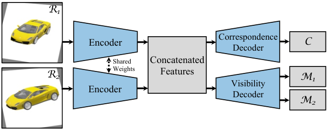
Encoders. The main role of encoders shown in Fig. 3 is to encode correlations between two input images $\mathcal{R}_{1}$ and $\mathcal{R}_{2}$ into CNN features. There are two encoders sharing weights, each of which processes each of the rectified pair with convolution layers followed by ReLU and max pooling. The CNN features from the two encoders are concatenated channel-wise by the late fusion and fed into the correspondence decoder and visibility decoder.

Correspondence decoder. The correspondence decoder shown in Fig. 3 processes the concatenated encoder features by successive deconvolution layers as done in [4, 5, 31, 28, 35]. The last layer of the correspondence decoder is a convolution layer and outputs the dense correspondences $\mathcal{C}$ between $\mathcal{R}_{1}$ and $\mathcal{R}_{2}$. As $\mathcal{R}_{1}$ and $\mathcal{R}_{2}$ are already rectified by the rectification network, the predicted correspondences are only 1D, i.e., correspondences along the same rows.

Assume that $\mathcal{C}$ is defined with respect to the pixel coordinates $p$ of $\mathcal{R}_{1}$. We can then represent the point correspondence sets $P_{1}=\{p_{1}^{1},\ldots,p_{1}^{M}\}$ and $P_{2}=\{p_{2}^{1},\ldots,p_{2}^{M}\}$ as

where $M$ is the number of pixels in $\mathcal{R}_{1}$. With these $P_{1}$ and $P_{2}$, we can now synthesize a middle view $\mathcal{R}_{\alpha=0.5}$ by (1).

In (1), obtaining $\mathcal{R}_{2}(p_{2}^{i})$ needs interpolation because $p_{2}^{i}=p^{i}+\mathcal{C}(p^{i})$ are generally non-integer valued. Such interpolation can be done very efficiently as it is sampling from regular grids. We also need to sample $\mathcal{R}_{\alpha=0.5}(q)$ on regular grid coordinates $q$ from $\mathcal{R}_{\alpha=0.5}(0.5p_{1}^{i}+0.5p_{2}^{i})$ as $0.5p_{1}^{i}+0.5p_{2}^{i}$ are non-integer valued. Unlike $\mathcal{R}_{2}(p_{2}^{i})$, sampling $\mathcal{R}_{\alpha=0.5}(q)$ from $\mathcal{R}_{\alpha=0.5}(0.5p_{1}^{i}+0.5p_{2}^{i})$ can be tricky because it is sampling from irregularly placed samples.

To overcome this issue of sampling from irregularly placed samples, we can define $\mathcal{C}$ differently: $\mathcal{C}$ is defined with respect to the pixel coordinates $q$ of $\mathcal{R}_{\alpha=0.5}$. That is, the point correspondence sets $P_{1}$ and $P_{2}$ are obtained as

Then the middle view $\mathcal{R}_{\alpha=0.5}$ can be easily synthesized as

where both $\mathcal{R}_{1}(P_{1})$ and $\mathcal{R}_{2}(P_{2})$ can be efficiently sampled.

Figure 4 shows an example of the dense correspondences between $\mathcal{R}_{1}$ and $\mathcal{R}_{2}$ predicted by the correspondence decoder. It is notable that the predicted correspondences are highly accurate even for textureless regions.

Visibility decoder. It is not unusual for $\mathcal{R}_{1}$ and $\mathcal{R}_{2}$ to have different visibility patterns as shown in Fig. 5(a). In such cases, the correspondences of pixels only visible in either one of views are ill-defined and thus cannot be predicted correctly. The undesirable consequence of using (4) with all of the correspondences for such cases is severe ghosting artifacts as shown in Fig. 5(b).

In order to solve this issue, we adopt the idea to use blending masks proposed in [35]. We use the visibility decoder shown in Fig. 3 to predict visibility of each pixel of $\mathcal{R}_{1}(P_{1})$ and $\mathcal{R}_{2}(P_{2})$ in the synthesized view $\mathcal{R}_{\alpha=0.5}$. The visibility decoder processes the concatenated encoder features by successive deconvolution layers. At the end of the visibility decoder, a convolution layer outputs 1-channel feature map $\mathcal{M}$ that is converted to a blending mask $\mathcal{M}_{1}$ for $\mathcal{R}_{1}(P_{1})$ by a sigmoid function. A blending mask $\mathcal{M}_{2}$ for $\mathcal{R}_{2}(P_{2})$ is determined by $\mathcal{M}_{2}=1-\mathcal{M}_{1}$. $\mathcal{M}_{1}$ and $\mathcal{M}_{2}$ represent the probability of each pixel of $\mathcal{R}_{1}(P_{1})$ and $\mathcal{R}_{2}(P_{2})$ to appear in the synthesized view $\mathcal{R}_{\alpha=0.5}$.

Now we can synthesize the middle view $\mathcal{R}_{\alpha=0.5}$ using all of the correspondences and $\mathcal{M}_{1}$ and $\mathcal{M}_{2}$ as

where $\odot$ represents element-wise multiplication. As shown in Fig 5(c), regions that should not appear in the middle view have very low values close to 0 (dark blue) in $\mathcal{M}_{1}$ and $\mathcal{M}_{2}$ while commonly visible regions have similar values around 0.5 (green and yellow). As a result, we can obtain ghosting-free $\mathcal{R}_{\alpha=0.5}$ by (5) as shown in Fig. 5(c).

Figure 6 shows the view morphing network. Sampling layers take in the dense correspondences $\mathcal{C}$ and the rectified pair $\mathcal{R}_{1}$ and $\mathcal{R}_{2}$, and output $\mathcal{R}_{1}(P_{1})$ and $\mathcal{R}_{2}(P_{2})$ in (5) by sampling pixel values of $\mathcal{R}_{1}$ and $\mathcal{R}_{2}$ at $P_{1}$ and $P_{2}$ determined by (3). Here, we can use 1D interpolation for the sampling because $\mathcal{C}$ represents 1D correspondences on the same rows. Then the blending layer synthesizes the middle view $\mathcal{R}_{\alpha=0.5}$ from $\mathcal{R}_{1}(P_{1})$ and $\mathcal{R}_{2}(P_{2})$ and their corresponding blending masks $\mathcal{M}_{1}$ and $\mathcal{M}_{2}$ by (5). The view morphing network does not have learnable weights as both sampling and blending are fixed operations.

All layers of DVM are differentiable and thus end-to-end-training with a single loss at the end comparing the synthesized middle view and ground truth middle view is possible. For training, we use the Euclidean loss defined as

where $\mathcal{R}_{\textrm{GT}}$ is the desired ground truth middle view image and $M$ is the number of pixels. Note that we do not need the post-warping step as in [26] (Section 2.3) because the rectification network is trained to rectify $\mathcal{I}_{1}$ and $\mathcal{I}_{2}$ so that the middle view of $\mathcal{R}_{1}$ and $\mathcal{R}_{2}$ can be directly matched against the desired ground truth middle view $\mathcal{R}_{\textrm{GT}}$.

The CNN architecture details of DVM such as number of layers and kernel sizes and other implementation details are shown in Appendix A. With Intel Xeon E5-2630 and a single Nvidia Titan X, DVM processes a batch of 20 input pairs of $224\times 224$ in 0.269 secs using the modified version of Caffe [17].

Training data. We used “Car”, “Chair”, “Airplane”, and “Vessel” of ShapeNet to create training data. We randomly split all 3D models of each category into $80\%$ training and $20\%$ test instances. We rendered each model using Blender (https://www.blender.org) using cameras at azimuths of $0^{\circ}$ to $355^{\circ}$ with $5^{\circ}$ steps and elevations of $0^{\circ}$ to $30^{\circ}$ with $10^{\circ}$ steps with the fixed distance to objects. We finally cropped object regions using the same central squares for all viewpoints and resized them to $224\times 224$.

We created training triplets $\{\mathcal{I}_{1},\mathcal{R}_{\textrm{GT}},\mathcal{I}_{2}\}$ where $\mathcal{I}_{1}$, $\mathcal{R}_{\textrm{GT}}$, and $\mathcal{I}_{2}$ have the same elevations. Let $\phi_{1}$, $\phi_{2}$, and $\phi_{\textrm{GT}}$ denote azimuths of $\mathcal{I}_{1}$, $\mathcal{I}_{2}$, and $\mathcal{R}_{\textrm{GT}}$. We first sampled $\mathcal{I}_{1}$ with $\phi_{1}$ multiples of $10^{\circ}$, and sampled $\mathcal{I}_{2}$ to satisfy $\Delta\phi=\phi_{2}-\phi_{1}=\{20^{\circ},30^{\circ},40^{\circ},50^{\circ}\}$. $\mathcal{R}_{\textrm{GT}}$ is then selected to satisfy $\phi_{\textrm{GT}}-\phi_{1}=\phi_{2}-\phi_{\textrm{GT}}=\{10^{\circ},15^{\circ},20^{\circ},25^{\circ}\}$. We provided VSAF with 8D one-hot vectors [35] to represent viewpoint transformations from $\mathcal{I}_{1}$ to $\mathcal{R}_{\textrm{GT}}$ and from $\mathcal{I}_{2}$ to $\mathcal{R}_{\textrm{GT}}$ equivalent to azimuth differences of $\{\pm 10^{\circ},\pm 15^{\circ},\pm 20^{\circ},\pm 25^{\circ}\}$. The number of training triplets for “Car”, “Chair”, “Airplane”, and “Vessel” are about 3.4M, 3.1M, 1.9M, and 0.9M, respectively. More details of the ShapeNet training data are shown in Appendix C.

Category-specific training. We first show view synthesis results of DVM and VSAF trained on each category separately. Both DVM and VSAF were trained using exactly the same training data. For evaluating the view synthesis results, we randomly sampled 200,000 test triplets for each category created with the same configuration as that of the training triplets. As an error metric, we use the mean squared error (MSE) between the synthesized output and ground truth summed over all pixels.

Figure 7 shows qualitative comparisons of view synthesis results by DVM and VSAF. It is clear that view synthesis results by DVM are visually more pleasing with much less ghosting artifacts and much closer to the ground truth views than those by VSAF. Table 1 shows the mean of MSE by DVM and VSAF for each category. The mean of MSE by DVM are considerably smaller than those by VSAF for all four categories, which matches well the qualitative comparisons in Fig. 7 . The mean of MSE by DVM for “Car”, “Chair”, “Airplane”, and “Vessel” are $63.8\%$, $43.5\%$, $47.6\%$, and $44.5\%$ of that by VSAF, respectively.

Figure 8 shows the rectification results and dense correspondences obtained by DVM for the test input images shown in Fig. 7. Note that DVM yields highly accurate rectification results and dense correspondence results. In fact, it is not possible to synthesize the middle view accurately if one of them is incorrect. The quantitative analysis of the rectification accuracy by DVM is shown in Appendix C.

Figure 9 shows plots of mean of MSE by DVM and VSAF as a function of $\phi_{1}$ (azimuth of $\mathcal{I}_{1}$) where different line colors represent different azimuth differences $\Delta\phi$ between $\mathcal{I}_{1}$ and $\mathcal{I}_{2}$. As expected, the mean of MSE increases as $\Delta\phi$ increases. Note that the mean of MSE by DVM for $\Delta\phi=50^{\circ}$ is similar to that by VSAF for $\Delta\phi=30^{\circ}$. Also note that the mean of MSE by DVM for each $\Delta\phi$ has peaks near $\phi_{1}=90^{\circ}\cdot i-\Delta\phi/2,i=0,1,2,3$, where there is considerable visibility changes between $\mathcal{I}_{1}$ and $\mathcal{I}_{2}$, e.g., from a right-front view $\mathcal{I}_{1}$ to a left-front view $\mathcal{I}_{2}$.

We also compare the performance of DVM and VSAF trained for the larger azimuth differences up to $90^{\circ}$. Due to the limited space, the results are shown in Appendix C.

Robustness test. We now test the robustness of DVM and VSAF to inputs that have different azimuths and elevations from those of the training data. We newly created 200,000 test triplets of “Car” with azimuths and elevations that are $5^{\circ}$ shifted from those of the training triplets but still with $\Delta\phi=\{20^{\circ},30^{\circ},40^{\circ},50^{\circ}\}$. The mean of MSE for the $5^{\circ}$ shifted test triplets by DVM and VSAF are 71.75 and 107.64, respectively. Compared to the mean of MSE by DVM and VSAF on the original test triplets of “Car” in Tab. 1, both DVM and VSAF performed worse similarly: $61\%$ MSE increase by DVM and $54\%$ MSE increase by VSAF. However, note that the mean of MSE by DVM on the $5^{\circ}$ shifted test triplets (71.75) is similar to that by VSAF on the original test triplets (70.11).

We also test the robustness of DVM and VSAF to inputs with azimuth differences $\Delta\phi$ that are different from those of the training data. We newly created 500,000 test triplets of “Car” with $\mathcal{I}_{1}$ that are the same as the training triplets and $\mathcal{I}_{2}$ and $\mathcal{R}_{\textrm{GT}}$ corresponding to $15^{\circ}\leq\Delta\phi<60^{\circ}$ with $2.5^{\circ}$ steps. We provided VSAF with 8D one-hot vectors by finding the elements from $\{\pm 10^{\circ},\pm 15^{\circ},\pm 20^{\circ},\pm 25^{\circ}\}$ closest to $\phi_{1}-\phi_{\textrm{GT}}$ and $\phi_{2}-\phi_{\textrm{GT}}$.

Figure 10 shows plots of mean of MSE by DVM and VSAF for the new 500,000 test triplets of “Car”. It is clear that DVM is much more robust to the unseen $\Delta\phi$ than VSAF. VSAF yielded much higher MSE for the unseen $\Delta\phi$ compared to that for $\Delta\phi$ multiples of 10. Contrarily, the MSE increase by DVM for such unseen $\Delta\phi$ is minimal except for $\Delta\phi>50^{\circ}$. This result suggests that DVM which directly considers two input images together for synthesis without relying on the viewpoint transformation inputs has more generalizability than VSAF.

Category-agnostic training. We now show view synthesis results of DVM and VSAF trained in a category-agnostic way, i.e., we trained DVM and VSAF using all training triplets of all four categories altogether. For this category-agnostic training, we limited the maximum number of training triplets of each category to 1M. For testing, we additionally selected four unseen categories from ShapeNet: “Motorcycle”, “Laptop”, “Clock”, and “Bookshelf”. The test triplets of the unseen categories were created with the same configuration as that of the training triplets.

Figure 11 shows qualitative comparisons of view synthesis results by DVM and VSAF on the unseen categories. We can see the view synthesis results by DVM are still highly accurate even for the unseen categories. Especially, DVM even can predict the blending masks correctly as shown in Fig. 11(d). Contrarily, VSAF yielded view synthesis results with lots of ghosting artifacts and severe shape distortions.

Table 2 shows the mean of MSE by DVM and VSAF trained in a category-agnostic way. Compared to Tab. 1, we can see the mean of MSE by both DVM and VSAF for “Car”, “Chair”, and “Airplane” slightly increased due to less training samples of the corresponding categories. Contrarily, the mean of MSE by both DVM and VSAF for “Vessel” decreased mainly due to the training samples of the other categories. The performance difference between DVM and VSAF for the unseen categories is much greater than that for the seen categories. The mean of MSE by DVM for “Motorcycle”, “Laptop”, “Clock”, and “Bookshelf” are $32.9\%$, $39.0\%$, $43.5\%$, and $33.0\%$ of that by VSAF, respectively. These promising results by DVM on the unseen categories suggest that DVM can learn general features necessary for rectifying image pairs and establishing correspondences between them. The quantitative analysis of the rectification accuracy by DVM for the unseen categories is shown in Appendix C.

Training data. Multi-PIE dataset [10] contains face images of 337 subjects captured at 13 viewpoints from $0^{\circ}$ to $180^{\circ}$ azimuth angles. We split 337 subjects into 270 training and 67 test subjects. We used 11 viewpoints from $15^{\circ}$ to $165^{\circ}$ because images at $0^{\circ}$ and $180^{\circ}$ have drastically different color characteristics. We sampled $\mathcal{I}_{1}$ and $\mathcal{I}_{2}$ to have $\Delta\phi=\{30^{\circ},60^{\circ}\}$, and picked $\mathcal{R}_{\textrm{GT}}$ to satisfy $\phi_{\textrm{GT}}-\phi_{1}=\phi_{2}-\phi_{\textrm{GT}}=\{15^{\circ},30^{\circ}\}$. The number of training triplets constructed in this way is 643,760. We provided VSAF with 4D one-hot vectors accordingly.

Multi-PIE provides detailed facial landmarks annotations but only for subsets of whole images. Using those annotations, we created two sets of training data with (i) loose and (ii) tight facial region crops. For the loose crops, we used a single bounding box for all images of the same viewpoint that encloses all facial landmarks of those images. For the tight crops, we first performed face segmentation using FCN [23] trained with convex hull masks of facial landmarks. We then used a bounding box of the segmented region for each image. For both cases, we extended bounding boxes to be square and include all facial regions and finally resized them to $224\times 224$.

Results. We trained DVM and VSAF using each of the two training sets separately. For testing, we created two sets of 157,120 test triplets from 67 test subjects, one with the loose crops and the other with the tight crops, with the same configuration as that of the training sets.

Figure 12(a) shows qualitative comparisons of view synthesis results by DVM and VSAF on the test triplets with the loose facial region crops. The view synthesis results by VSAF suffer lots of ghosting artifacts and severe shape distortions mainly because (i) faces are not aligned well and (ii) their scales can be different. Contrarily, DVM yielded very satisfactory view synthesis results by successfully dealing with the unaligned faces and scale differences thanks to the presence of the rectification network. These successful view synthesis results by DVM have significance in that DVM can synthesize novel views quite well even with the the camera setup not as precise as that of the ShapeNet rendering and objects with different scales.

Figure 12(b) shows qualitative comparisons of view synthesis results by DVM and VSAF on the test triplets with the tight facial region crops. The view synthesis results by VSAF are much improved compared to the case of the loose facial region crops because the facial regions are aligned fairly well and their scale differences are negligible. However, the view synthesis results by DVM are still better than those by VSAF with less ghosting artifacts and less shape distortions. Table 3 shows the mean of MSE by DVM and VSAF for the Multi-PIE test triplets that match well the qualitative comparisons in Fig. 12.

Figure 13 shows the intermediate view synthesis results obtained by linearly interpolating the blending masks $\mathcal{M}_{1}$ and $\mathcal{M}_{2}$ as well as $\mathcal{R}_{1}$ and $\mathcal{R}_{2}$. As the dense correspondences predicted by DVM are highly accurate, we can synthesize highly realistic intermediate views. The detailed procedure to synthesize the intermediate views and more results are shown in Appendix C.

Table 4 shows the CNN architecture details of the rectification network with both early and late fusions. For the case of the early fusion, $\mathcal{S}_{I}$ represents the channel-wise concatenation of the two input images $\mathcal{I}_{1}$ and $\mathcal{I}_{2}$. The output of “RC8” is a 18D vector that is split into two 9D vectors to represent $H_{1}$ and $H_{2}$ that are fed into the geometric transformation layers. For the case of the late fusion, $\mathcal{I}_{1}$ and $\mathcal{I}_{2}$ are processed separately by two convolution towers sharing weights (thus the same convolution tower actually) and their CNN features are fused by the channel-wise concatenation. For the convolution tower for $\mathcal{I}_{1}$, “RP5-1-2” is the channel-wise concatenation in the order of the output of “RP5-1” and output of “RP5-2”. Similarly, for the convolution tower for $\mathcal{I}_{2}$, “RP5-2-1” is the channel-wise concatenation in the order of the output of “RP5-2” and output of “RP5-1”. By further processing these concatenated features, each convolution tower outputs a 9-D homography vector at the end (“RC8-1” and “RC8-2”).

Table 5 shows the CNN architecture details of the encoder with both early and late fusions. For the case of the early fusion, $\mathcal{S}_{R}$ represents the channel-wise concatenation of the rectified pair $\mathcal{R}_{1}$ and $\mathcal{R}_{2}$. The output of “EC6” is the CNN features that are fed into the decoders. For the case of the late fusion, $\mathcal{R}_{1}$ and $\mathcal{R}_{2}$ are processed separately by two encoder towers sharing weights (thus the same encoder tower actually) and their CNN features are fused by the channel-wise concatenation (“EC6-1-2”). “EC3-1-2”, “EC4-1-2”, “EC5-1-2” are the channel-wise concatenation of CNN features from the lower convolution layers that are used by the visibility decoder.

Table 6 shows the CNN architecture details of the correspondence decoder and visibility decoder. The correspondence decoder first processes the output of “EC6” or “EC6-1-2” by the two convolution layers depending on whether the early or late fusion is used in the encoder. Then the five deconvolution layers perform upsampling of the CNN features. A convolution layer at the end (“CC3”) finally outputs the 1D dense correspondence $\mathcal{C}$. In order to increase the accuracy of the predicted dense correspondences, we use the CNN features from the lower convolution layers of the encoder together with those from the last convolution layer of the encoder. We obtain “EC3-feature”, “EC4-feature”, and “EC5-feature” by applying $1\times 1$ kernels to the output of “EC3” or “EC3-1-2”, “EC4” or “EC4-1-2”, and “EC5” or “EC5-1-2”, respectively, depending on whether the early or late fusion is used in the encoder. These are then concatenated to the output of “CD1”, “CD2”, and “CD3” appropriately (“CD1-EC5-feature”, “CD2-EC4-feature”, and “CD3-EC3-feature”).

The visibility decoder is basically the same as the correspondence decoder except it uses the smaller number of channels and it does not use the CNN features from the lower convolution layers of the encoder. The output of the last convolution layer (“VC3”) is transformed to the blending mask $\mathcal{M}_{1}$ by the sigmoid function (“VC3-sig”). Another blending mask $\mathcal{M}_{2}$ is determined by $1-\mathcal{M}_{1}$.

We performed experiments to test all possible combinations of the early and late fusions in the rectification and encoder-decoder networks to find the best one for our view synthesis problem. There are four possible cases: (i) early fusions in both the rectification and encoder-decoder networks, (ii) early fusion in the rectification network and late fusion in the encoder-decoder network, (iii) late fusion in the rectification network and early fusion in the encoder-decoder network, and (iv) late fusions in both the rectification and encoder-decoder networks.

Table. 7 shows the mean of MSE for “Car” by DVM with the four cases considered. Although it is difficult to draw any generalizable conclusions from Tab. 7, at least it explains our CNN architecture design choice: the early fusion in the rectification network and late fusion in the encoder-network yields the best results for our view synthesis problem.

We set the spatial dimensions of $\mathcal{I}_{1}$, $\mathcal{I}_{2}$, $\mathcal{R}_{1}$, $\mathcal{R}_{2}$, and $\mathcal{R}_{\alpha=0.5}$ all to be $224\times 224$. We normalize each channel of $\mathcal{I}_{1}$ and $\mathcal{I}_{2}$ to the range of $-0.5$ to $0.5$ by global shift by 128 and division by 255. We use 2D bilinear interpolation for the geometric transformation layers in the rectification network and 1D linear interpolation for the sampling layers in the view morphing network.

More details of training and test data. Table 8 shows the details of the ShapeNet training and test data of “Car”, “Chair”, “Airplane”, and “Vessel” used for evaluating the category-specific training results while Tab. 9 shows the details of the unseen ShapeNet test data of “Motorcycle”, “Laptop”, “Clock”, and “Bookshelf” used for evaluating the category-agnostic training results.

More qualitative results. Figure 14 to Fig. 17 show more qualitative comparisons of the view synthesis results on “Car”, “Chair”, “Airplane”, and “Vessel” of ShapeNet by DVM and VSAF [35] trained in a category-specific way. Figure 18 shows more examples of the rectification results and dense correspondence results by DVM.

Figure 19 to Fig. 22 show more qualitative comparisons of the view synthesis results on the unseen “Motorcycle”, “Laptop”, “Clock”, and “Bookshelf” of ShapeNet by DVM and VSAF trained in a category-agnostic way. Figure 23 shows examples of the rectification results and dense correspondence results by DVM on the unseen categories.

Rectification accuracy. The rectification network is trained to rectify $\mathcal{I}_{1}$ and $\mathcal{I}_{2}$ so that the middle view of $\mathcal{R}_{1}$ and $\mathcal{R}_{2}$ can be directly matched against the desired ground truth middle view $\mathcal{R}_{\textrm{GT}}$. We can measure how successful the rectification is by checking how well aligned the known points in the ground truth middle view are to the corresponding points in the rectified pair $\mathcal{R}_{1}$ and $\mathcal{R}_{2}$.

Let $T_{1}$, $T_{\textrm{GT}}$, and $T_{2}$ denote the known camera poses used for rendering a test triplet $\{\mathcal{I}_{1},\mathcal{R}_{\textrm{GT}},\mathcal{I}_{2}\}$. In the camera coordinate frames of $T_{\textrm{GT}}$, we put four lines with end points $l_{1}^{i}$ and $l_{2}^{i},i=1,\ldots,4$, as

These lines will be projected onto the image plane of $T_{\textrm{GT}}$ as horizontal lines. Note that the distance from the camera to 3D models in rendering was 4.

As we know the exact intrinsic camera parameters used for rendering and the relative camera poses of $T_{1}$ and $T_{2}$ with respect to $T_{\textrm{GT}}$, we can obtain the projections of the four lines in (12) onto the image planes of $T_{1}$ and $T_{2}$. Before the rectification, these lines will be projected to the image planes of $T_{1}$ and $T_{2}$ as slanted. After applying the homographies $H_{1}$ and $H_{2}$ predicted by the rectification network to those projected lines of $T_{1}$ and $T_{2}$, they will be aligned well to the corresponding projected lines of $T_{\textrm{GT}}$.

As a measure for the rectification error, we compute the average vertical difference $D$ between the end points of the corresponding projected lines of $T_{\textrm{GT}}$ and $T_{1}$ and $T_{2}$ after the rectification. With $a_{0}^{i}$ and $a_{1}^{i}$ to represent $y$-components of projections of the end points in (12) onto the image plane of $T_{\textrm{GT}}$, we compute $D$ as

where $b_{0}^{i}$ and $b_{1}^{i}$ are $y$-components of the corresponding projections onto the image plane of $T_{1}$ after the rectification and $c_{0}^{i}$ and $c_{1}^{i}$ are those of $T_{2}$ also after the rectification.

Table 10 shows the mean of $D$ by DVM on the ShapeNet test triplets. Note that the rectification error by DVM for “Car”, “Chair”, “Airplane”, and “Vessel” is quite consistent for both category-specific training and category-agnostic training. Similarly to MSE of the view synthesis results, the rectification error for “Vessel” by the category-agnostic training is decreased by the training data of the other categories. It is significant that the rectification error for the unseen “Motorcycle”, “Laptop”, and “Bookshelf” are quite similar to that for the seen categories. The rectification error for the unseen “Clock” is relatively large, which leads to the relatively large MSE of the view synthesis results.

Larger azimuth differences. One can argue that VSAF is originally designed to be able to deal with larger azimuth differences. Therefore, we test the performance of DVM and VSAF for azimuth differences up to $90^{\circ}$. We trained DVM and VSAF using training triplets of “Car” newly created with $20^{\circ}\leq\Delta\phi\leq 90^{\circ}$ with $10^{\circ}$ steps. We provided VSAF with 16-D one-hot vectors as viewpoint transformation input.

Figure 24 shows the mean of MSE by DVM and VSAF on the test triplets of “Car” with $20^{\circ}\leq\Delta\phi\leq 90^{\circ}$ with $10^{\circ}$ steps. As long as DVM and VSAF are trained using the same data, DVM consistently outperforms VSAF even for larger azimuth differences up to $90^{\circ}$.

Figure 25 and Fig. 26 show more qualitative comparisons of the view synthesis results by DVM and VSAF on the Multi-PIE test data with the loose and tight facial region crops, respectively. Figure 27 shows examples of the rectification results and dense correspondence results by DVM on the Multi-PIE test input images.

Figure 28 shows examples of challenging cases for DVM. It is generally difficult for DVM to deal with highly complex thin structures as shown in Fig. 28(a). Plus, the current blending masks cannot properly deal with the different illumination and color characteristics between input images, and thus blending seams can be visible in some cases as shown in Fig. 28(b).

We synthesize $\mathcal{R}_{\alpha}$ for any $\alpha$ of between 0 and 1 as

where $w_{1}=\frac{(1-\alpha)\mathcal{M}_{1}(p_{1}^{i})}{(1-\alpha)\mathcal{M}_{1}(p_{1}^{i})+\alpha\mathcal{M}_{2}(p_{2}^{i})}$ and $w_{2}=1-w_{1}$. Note that we interpolate the blending masks $\mathcal{M}_{1}$ and $\mathcal{M}_{2}$ as well as $\mathcal{R}_{1}(P_{1})$ and $\mathcal{R}_{2}(P_{2})$.

These synthesized views represent intermediate views between $\mathcal{R}_{1}$ and $\mathcal{R}_{2}$. As what we want in practice is intermediate views between $\mathcal{I}_{1}$ to $\mathcal{I}_{2}$, it is necessary to apply post-warping accordingly. We specifically create two linear camera paths, one from $\mathcal{I}_{1}$ to $\mathcal{R}_{\alpha=0.5}$ and the other from $\mathcal{R}_{\alpha=0.5}$ to $\mathcal{I}_{2}$. We can represent $H_{1}$ and $H_{2}$ used for rectifying $\mathcal{I}_{1}$ and $\mathcal{I}_{2}$ as elements of the special linear group $SL(3)$ by normalizing them to have unit determinants [21]. Then the necessary post-warping homographies $H_{\alpha}$ for the linear camera paths can be determined as

where $\exp$ and $\log$ are matrix exponential and logarithm.

Figure 29 shows the intermediate view synthesis results obtained by (14) and (15). The second and third rows of Fig. 29 show the intermediate view synthesis results for the case of input with different instances of “Car”, which are quite satisfactory.

References

- [1] T. Beier and S. Neely. Feature-based image metamorphosis. In Proc. SIGGRAPH, 1992.
- [2] A. Chang, T. Funkhouser, L. Guibas, P. Hanrahan, Q. Huang, Z. Li, S. Savarese, M. Savva, S. Song, H. Su, J. Xia, L. Yi, and F. Yu. Shapenet: An information-rich 3d model repository. Technical report, arXiv:1512.03012, 2015.
- [3] S. E. Chen and L. Williams. View interpolation for image synthesis. In Proc. SIGGRAPH, 1993.
- [4] A. Dosovitskiy, P. Fischery, E. Ilg, C. Hazirbas, V. Golkov, P. van der Smagt, D. Cremers, T. Brox, et al. Flownet: Learning optical flow with convolutional networks. In Proc. ICCV, 2015.
- [5] A. Dosovitskiy, J. Springenberg, and T. Brox. Learning to generate chairs with convolutional neural networks. In Proc. CVPR, 2015.
- [6] J. Flynn, I. Neulander, J. Philbin, and N. Snavely. Deepstereo: Learning to predict new views from the world’s imagery. In Proc. ICCV, 2015.
- [7] Y. Furukawa and J. Ponce. Accurate, dense, and robust multiview stereopsis. IEEE Trans. Pattern Anal. Mach. Intell., 2010.
- [8] X. Glorot and Y. Bengio. Understanding the difficulty of training deep feedforward neural networks. In Proc. AISTATS, 2010.
- [9] S. J. Gortler, R. Grzeszczuk, R. Szeliski, and M. F. Cohen. The lumigraph. In Proc. SIGGRAPH, 1996.
- [10] R. Gross, I. Matthews, J. Cohn, T. Kanade, and S. Baker. Multi-pie. Image and Vision Computing, 2010.
- [11] R. Hartley and A. Zisserman. Multiple View Geometry in Computer Vision. Cambridge University Press, 2003.
- [12] J. Heinly, J. Schonberger, E. Dunn, and J.-M. Frahm. Reconstructing the world* in six days *(as captured by the yahoo 100 million image dataset). In Proc. CVPR, 2015.
- [13] G. Hinton, A. Krizhevsky, and S. Wang. Transforming auto-encoders. In Proc. ICANN, 2011.
- [14] D. Hoiem, A. Efros, and M. Hebert. Automatic photo pop-up. ACM transactions on graphics, 2005.
- [15] Y. Horry, K. Anjyo, and K. Arai. Tour into the picture: using a spidery mesh interface to make animation from a single image. In Proc. 24th annual conference on Computer graphics and interactive techniques, 1997.
- [16] M. Jaderberg, K. Simonyan, A. Zisserman, and K. Kavukcuoglu. Spatial transformer networks. In Proc. NIPS, 2015.
- [17] Y. Jia, E. Shelhamer, J. Donahue, S. Karayev, J. Long, R. Girshick, S. Guadarrama, and T. Darrell. Caffe: Convolutional architecture for fast feature embedding. Technical report, arXiv:1408.5093, 2014.
- [18] M. Jones and T. Poggio. Model-based matching of line drawings by linear combination of prototypes. In Proc. ICCV, 1995.
- [19] A. Katayama, K. Tanaka, T. Oshino, and H. Tamura. A viewpoint dependent stereoscopic display using interpolation of multi-viewpoint images. Stereoscopic Displays and Virutal Reality Systems, 1995.
- [20] D. Kingma, J. Ba, and G. Gamow. Adam: A method for stochastic optimization. Technical report, arXiv:1412.6980, 2014.
- [21] J. Kwon, H. Lee, F. Park, and K. Lee. A geometric particle filter for template-based visual tracking. IEEE Trans. Pattern Anal. Mach. Intell., 2014.
- [22] M. Levoy and P. Hanrahan. Light field rendering. In Proc. SIGGRAPH, 1996.
- [23] J. Long, E. Shelhamer, and T. Darrel. Fully convolutional networks for semantic segmentation. In Proc. CVPR, 2015.
- [24] B. Oh, M. Chen, J. Dorsey, and F. Durand. Image-based modeling and photo editing. In Proc. 28th annual conference on Computer graphics and interactive techniques, 2001.
- [25] E. Park, J. Yang, E. Yumer, D. Ceylan, and A. C. Berg. Transformation-grounded image generation network for novel 3d view synthesis. In Proc. CVPR, 2017.
- [26] S. Seitz and C. Dyer. View morphing. In Proc. SIGGRAPH, 1996.
- [27] A. Shashua. Algebraic functions for recognition. IEEE Trans. Pattern Anal. Mach. Intell., 1995.
- [28] M. Tatarchenko, A. Dosovitskiy, and T. Brox. Multi-view 3d models from single images with a convolutional network. In Proc. ECCV, 2016.
- [29] T. Vetter and T. Poggio. Linear object classes and image synthesis from a single example image. IEEE Trans. Pattern Anal. Mach. Intell., 1997.
- [30] C. Wu. Towards linear-time incremental structure from motion. In Proc. 3DV, 2013.
- [31] J. Yang, S. Reed, M. Yang, and H. Lee. Weakly-supervised disentangling with recurrent transformations for 3d view synthesis. In Proc. NIPS, 2015.
- [32] L. Zhang, G. Dugas-Phocion, J. Samson, and S. Seitz. Single-view modelling of free-form scenes. The Journal of Visualization and Computer Animation, 2002.
- [33] E. Zheng, E. Dunn, V. Jojic, and J.-M. Frahm. Patchmatch based joint view selection and depthmap estimation. In Proc. CVPR, 2014.
- [34] E. Zheng and C. Wu. Structure from motion using structure-less resection. In Proc. ICCV, 2015.
- [35] T. Zhou, S. Tulsiani, W. Sun, J. Malik, and A. A. Efros. View synthesis by appearance flow. In Proc. ECCV, 2016.
Appendix A. CNN architecture details
We present the CNN architecture details of each sub-network of Deep View Morphing. Note that only layers with learnable weights are shown here. As aforementioned in Section 3 of the main paper, we can consider the early and late fusions in the rectification network and encoder-decoder network. We define the early fusion as channel-wise concatenation of two input images while the late fusion as channel-wise concatenation of CNN features of the two input images processed by convolution layers.
A.1. Rectification network