Probabilistic reduced-order modeling for stochastic partial differential equations
Abstract
We discuss a Bayesian formulation to coarse-graining (CG) of PDEs where the coefficients (e.g. material parameters) exhibit random, fine scale variability. The direct solution to such problems requires grids that are small enough to resolve this fine scale variability which unavoidably requires the repeated solution of very large systems of algebraic equations.
We establish a physically inspired, data-driven coarse-grained model which learns a low-dimensional set of microstructural features that are predictive of the fine-grained model (FG) response. Once learned, those features provide a sharp distribution over the coarse scale effective coefficients of the PDE that are most suitable for prediction of the fine scale model output.
This ultimately allows to replace the computationally expensive FG by a generative probabilistic model based on evaluating the much cheaper CG several times. Sparsity enforcing priors further increase predictive efficiency and reveal microstructural features that are important in predicting the FG response. Moreover, the model yields probabilistic rather than single-point predictions, which enables the quantification of the unavoidable epistemic uncertainty that is present due to the information loss that occurs during the coarse-graining process.
keywords
Reduced-order modeling, generative Bayesian model, SPDE, effective material propertiesConstantin Grigo and Phaedon-Stelios Koutsourelakis
1 INTRODUCTION
Many engineering design problems such as flow in porous media and mechanical properties of composite materials require simulations that are capable of resolving the microstructure of the underlying medium. If the material components under consideration exhibit fine-scale heterogeneity, popular discretization schemes (e.g. finite elements) yield very large systems of algebraic equations. Pertinent solution strategies at best (e.g. multigrid methods) scale linearly with the dimension of the unknown state vector. Despite the ongoing improvements in computer hardware, repeated solutions of such problems, as is required in the context of uncertainty quantification (UQ), poses insurmountable difficulties.
It is obvious that viable strategies for such problems, as well as a host of other deterministic problems where repeated evaluations are needed such as inverse, control/design problems etc, should focus on methods that exhibit sublinear complexity with respect to the dimension of the original problem. In the context of UQ a popular and general such strategy involves the use of surrogate models or emulators which attempt to learn the input-output map implied by the fine-grained model. Such models, e.g. Gaussian Processes [26], polynomial chaos expansions [8], neural nets [2] and many more, are trained on a finite set of fine-grained model runs. Nevertheless, their performance is seriously impeded by the curse of dimensionality, i.e. they usually become inaccurate for input dimensions larger than a few tens or hundreds, or equivalently, the number of FG runs required to achieve an acceptable level of accuracy grows exponentially fast with the input dimension.
Alternative strategies for high-dimensional problems make use of multi-fidelity models [10, 16] as inexpensive predictors of the FG output. As shown in [12], lower-fidelity models whose output deviates significantly from that of the FG can still yield accurate estimates with significant computational savings, as long as the outputs of the models exhibit statistical dependence. In the case of PDEs where finite elements are employed as the FG, multi-fidelity solvers can be simply obtained by using coarser discretizations in space or time. While linear and nonlinear dimensionality reduction techniques are suitable for dealing with high-dimensional inputs [14], it is known which of the microstructural features are actually predictive of FG outputs [22].
The model proposed in the present paper attempts to address this question. By using a two-component Bayesian network, we are able to predict fine-grained model outputs based on only a finite number of training data runs and a repeated solution of a much coarser model. Uncertainties can be easily quantified as our model leads to probabilistic rather than point-like predictions.
2 THE FINE-GRAINED MODEL
Let be a probability space. Let be the Hilbert space of functions defined over the domain over which the physical problem is defined. We consider problems in the context of heterogeneous media which exhibit properties given by a random process defined over the product space . The corresponding stochastic PDE may be written as
| (1) |
where is a stochastic differential operator and , are elements of
the physical domain and the sample space, respectively. Discretization of the random process
as well as the
governing equation leads to a system of (potentially nonlinear) algebraic equations, which can be written in
residual form as
| (2) |
where is the -dimensional discretized solution vector for a given
and
the discretized residual vector. It is the model described by equation (2) which is denoted as the fine-grained
model (FG) henceforth.
3 A GENERATIVE BAYESIAN SURROGATE MODEL
Let
| (3) |
be the density of . The density of the fine-scale response is then given by
| (4) |
where the conditional density degenerates to a when the only uncertainties in the problem are due to .
The objective of this paper is to approximate this input-output map implied by , or equivalently in terms of probability densities, the conditional distribution . The latter case can also account for problems where additional sources of uncertainty are present and the input-output map is stochastic. To that end, we introduce a coarse-grained model (CG) leading to an approximate distribution which will be trained on a limited number of FG solutions .
Our approximate model employs a set of latent [3], reduced, collective variables which we denote by for reasons that will be apparent in the sequel, such that
| (5) |
As it can be understood from the equation above, the latent variables act as a probabilistic filter (encoder) on the FG input , retaining the features necessary for predicting the FG output . In order for to approximate well , the latent variables should not simply be the outcome of a dimensionality reduction on . Even if is amenable to such a dimensionality reduction, it is not necessary that the found would be predictive of . Posed differently, it is not important that provides a high-fidelity encoding of but it suffices that it is capable of providing a good prediction of the corresponding .
The aforementioned desiderata do not unambiguously define the form of the encoding/ decoding densities in (5) nor the type/dimension of the latent variables . In order to retain some of the physical and mathematical structure of the FG, we propose employing a coarsened, discretized version of the original continuous equation (1). In residual form this can again be written as
| (6) |
where is the -dimensional () discretized solution and is the discretized residual vector. Due to the significant discrepancy in dimensions , the cost of solving the CG in (6) is negligible compared to the FG in (2).
It is clear that plays the role of effective/equivalent properties but it is not obvious (except for some limiting cases where homogenization results can be invoked [23]) how these should depend on the fine-scale input nor how the solution of the CG should relate to in (2). Furthermore, it is important to recognize a priori that the use of the reduced variables in combination with the coarse model in (6) would in general imply some information loss. The latter should introduce an additional source of uncertainty in the predictions of the fine-scale output [25], even in the limit of infinite training data. For that purpose and in agreement with (5), we propose a generative probabilistic model composed of the following two densities:
- •
A probabilistic mapping from to , which determines the effective properties given . We write this as where denotes a set of model parameters,
- •
A coarse-to-fine map , which is the PDF of the FG output given the output of the CG. It is parametrized by .
This model is illustrated graphically in Figure 1. The density encodes into and the coarse-to-fine map plays the role of a decoder, i.e. given the CG output , it predicts .
Using the abbreviated notation , from (5) we obtain
| (7) |
where is the solution vector to equation (6). The previous discussion suggests the following generative process for drawing samples from i.e. predicting the FG output given a FG input ,
- •
draw a sample ,
- •
solve the CG to obtain ,
- •
draw a sample .
3.1 Model training
In order to train the model described above, it is a reasonable strategy to minimize the Kullback-Leibler divergence [5] between the target density and . As these are conditional distributions, the KL divergence would depend on . In order to calibrate the model for the values that are of significance, we operate on the augmented densities and , where is defined by (3). In particular, we propose minimizing with respect to
| (8) |
where is the number of training samples drawn from , i.e.
| (9) |
and is the entropy of that is nevertheless independent of the model parameters . It is obvious from the final expression in (8) that is a -likelihood function of the data which we denote by . In a fully Bayesian setting, this can be complemented with a prior leading to the posterior
| (10) |
It is up to the analyst if predictions using equation (7) are carried out using point estimates of (e.g. maximum likelihood (MLE) or maximum a posteriori (MAP)) or if a fully Bayesian approach is followed by averaging over the posterior . The latter has the added advantage of quantifying the uncertainty introduced due the finite training data . We pursue the former in the following as it is computationally more efficient.
3.1.1 Maximizing the posterior
Our objective is to find which maximizes the posterior given in equation (10), i.e.
| (11) |
The main difficulty in this optimization problem arises from the log-likelihood term which involves the log of an analytically intractable integral with respect to since
| (12) |
where we note that an independent copy of pertains to each data point . Due to this integration, typical deterministic optimization algorithms are not applicable.
However, as appears as a latent variable, we may resort to the well-known Expectation-Maximization algorithm [6]. Using Jensen’s inequality, we establish a lower bound on every single term of the sum in the log-likelihood by employing an arbitrary density (different for each sample ) as
| (13) |
Hence, the -posterior in (10) can be lower bounded by
| (14) |
The introduction of the auxiliary densities suggests the following recursive procedure [4] for maximizing the log-posterior:
- E-step:
Given some in iteration , find the auxiliary densities that maximize ,
- M-step:
Given , find the parameters that maximize .
It can be readily shown that the optimal is given by
| (15) |
with which the inequality in (13) becomes an equality. In fact, both E- and M-steps can be relaxed to find suboptimal , which enables the application of approximate schemes such as e.g. Variational Inference (VI) [24, 9]. For the M-step, we may resort to any (stochastic) optimization algorithm [17] or, on occasion, closed-form updates might also be feasible.
4 SAMPLE PROBLEM: 2D STATIONARY HEAT EQUATION

As a sample problem, we consider the 2D stationary heat equation on the unit square
| (16) |
where represents the temperature field. For the boundary conditions, we fix the temperature in the upper left corner (see Figure 2) to and prescribe the heat flux on the remaining domain boundary .
We consider a binary random medium whose conductivity can take the values and . To define such a field we consider transformations of a zero-mean Gaussian process of the form [18, 13]
| (17) |
where the thresholding constant is selected so as to achieve the target volume fraction (or equivalently ) of the material with conductivity (or equivalently of ). In the following we use an isotropic squared-exponential covariance function for of the form
| (18) |
In the following studies, we used values .
Due to the small correlation length , we discretize the SPDE in Equation (16) using standard quadrilateral finite elements, leading to a linear system of algebraic equations. We choose the discretization mesh of the random process to coincide with the finite element discretization mesh of the SPDE, i.e. .
Samples are readily obtained by simulating realizations of the discretized Gaussian field, transforming them according to (17) and solving the discretized SPDE. Three such samples can be seen in Figure 2.
4.1 Model specifications
We define a coarse model employing quadrilateral elements, the conductivities of which are given by the vector . Since these need to be strictly positive, we operate instead on defined as
| (19) |
For each element of the coarse model/mesh, we assume that
| (20) |
where is the subset of the vector that belongs to coarse element and some feature functions of the underlying that we specify below. In a more compact form, we can write
| (21) |
where is an design matrix with and is a diagonal covariance matrix with components .
For the coarse-to-fine map , we postulate the relation
| (22) |
where are parameters to be learned from the data. The matrix is of dimension and is a positive definite covariance matrix of size . To reduce the large amount of free parameters in the model, we fix to express coarse model’s shape functions. Furthermore, we assume that where is the -dimensional vector of diagonal entries of the diagonal matrix . The aforementioned expression implies, on average, a linear relation between the fine and coarse model outputs, which is supplemented by the residual Gaussian noise implied by . The latter expresses the uncertainty in predicting the FG output when only the CG solution is available. We note that the relation in Equation (20) (i.e. and ) will be adjusted during training so that the model implied in Equation (22) represents the data as good as possible.
From equation (15), we have that
| (23) |
where with , we mean the -th component of the vector in brackets. For use in the M-step, we compute the gradients
| (24) | ||||
| (25) |
where . We can readily compute the roots to find the optimal . Furthermore, from we get
| (26) |
4.2 Feature functions
The framework advocated allows for any form and any number of feature functions in (20). Naturally such a selection can be guided by physical insight [11]. In practice, the feature functions we are using can be roughly classified into two different groups:
4.2.1 Effective-medium approximations
We consider existing effective-medium approximation formula that can be found in the literature [23] as ingredients for construction of feature functions in equation (20). The majority of commonly used such features only retain low-order topological information. only The following approximations to the effective property can be used as building blocks for feature functions in the sense that we can transform them nonlinearly such that . In particular, as we are modeling , we include feature functions of type .
Maxwell-Garnett approximation (MGA)
The Maxwell-Garnett approximation is assumed to be valid if the microstructure consists of a matrix phase and spherical inclusions that are small and dilute enough such that interactions between them can be neglected. another Moreover, the heat flux far away from any inclusion is assumed to be constant. Under such conditions, the effective conductivity can be approximated in 2D as
| (27) |
where the volume fraction is given by the fraction of phase elements in the binary vector .
Self-consistent approximation (SCA)
The self-consistent approximation (or Bruggeman
formula) was originally developed for effective electrical properties
of random microstructures. It also considers non-interacting spherical inclusions and follows from the assumption that
perturbations of the electric field due to the inclusions average to . In 2D, the formula reads
| (28) |
Note that the SCA exhibits phase inversion symmetry.
Differential effective medium (DEM)
From a first-order expansion in volume fraction of the effective conductivity in the dilute limit of spherical inclusions, one can deduce the differential equation [23]
| (29) |
which can be integrated to
| (30) |
We solve for and use it as a feature function .
4.2.2 Morphology-describing features
Apart from the effective-medium approximations which only take into account the phase conductivities and volume fractions, we wish to have feature functions that more thoroughly describe the morphology of the underlying microstructure. Popular members of this class of microstructural features are the two-point correlation, the lineal-path function, the pore-size density or the specific surface to mention only a few of them [23].
We are however free to use any function as a feature, no matter from which field or consideration it may originate. We thus make use of existing image processing features [15] as well as novel topology-describing functions. Some important examples are
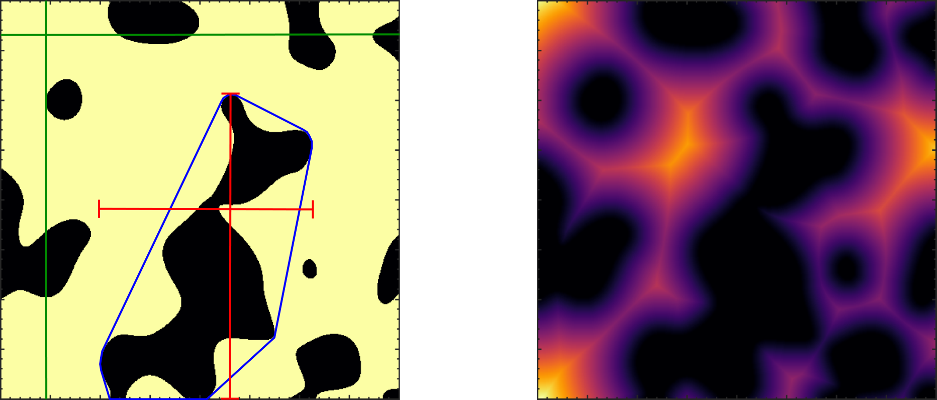
Convex area of connected phase blobs
This feature identifies distinct, connected “blobs” of only high or low conducting phase pixels and computes the area of the convex hull to each blob. We then can e.g. use the mean or maximum value thereof as a feature function.
Blob extent
From an identified phase blob, we can compute its maximum extension in - and -directions. One can for instance take the mean or maximum of maximum extension among identified blobs as a feature.
Distance transformation functions
The distance transform of a binary image assigns a number to each pixel that is the distance from that pixel to the nearest nonzero pixel in the binary image, see right part of Figure 3. One can use either phase to correspond to nonzero in the binary image as well as different distance metrics. As a feature, one can e.g. take the mean or maximum of the distance transformed image.
Pixel-cross function
This feature counts the number of high or low conducting pixels one has to cross going on a straight line from boundary to boundary in - or -direction. One can again take e.g. mean, maximum or minimum values as the feature function outputs.
Straight path mean function
A further refinement of the latter function is to take generalized means instead of numbers of crossed pixels along straight lines from boundary to boundary. In particluar, we use harmonic, geometric and arithmetic means as features.
4.3 Sparsity priors
It is clear from the previous discussion that the number of feature functions is practically limitless. The more such one introduces, the more unknown parameters must be learned. From the modeling point of view, while ML estimates can always be found, it is desirable to have as clear of a distinction as possible between relevant and irrelevant features that could provide further insight as well being able to do so with the fewest possible training data available. For that purpose we advocate the use of sparsity-enforcing priors in [1, 7, 19]. From a statistical perspective, this is also motivated by the bias-variance-tradeoff. Model prediction accuracy is adversely affected by two factors: One is noise in the training data (variance), the other is due to overly simple model assumptions (bias). Maximum-likelihood estimates of model parameters tend to have low bias but high variance, i.e. they accurately predict the training data but generalize poorly. To address this issue, a common Bayesian approach to control model complexity is the use of priors, which is the equivalent to regularization in frequentist formulations. A particularly appealing family of prior distributions is the Laplacian (or LASSO regression, [21]), as it sets redundant or unimportant predictors to exactly 0, thereby simplifying interpretation.
In particular, we use a prior on the coefficients of the form
| (31) |
with a hyper-parameter which can be set by either applying some cross-validation scheme or more efficiently by minimization of Stein’s unbiased risk estimate [20, 27]. A straightforward implementation of this prior is described in [7].
5 RESULTS
5.1 Required training data
We use a total number of 306 feature functions and a Laplacian prior (31) with a hyperparameter we find by cross-validation. We set the length scale parameter to and the expected volume fraction of the high conducting phase to . For the contrast, we take , where we set . The full- and reduced-order models are both computed on regular quadrilateral finite element meshes of size for the FG and , and for the CG.
Our goal is to measure the predictive capabilities of the described model. To that end, we compute the mean squared distance
| (32) |
of the predictive mean to the true FG output on a test set of samples. Predictions are carried out by drawing 10,000 samples of from the learned distribution , solving the coarse model and drawing a sample from for every test data point. Monte Carlo noise is small enough to be neglected.
As a reference value for the computed error , we compute the mean variance of the FG output
| (33) |
where expectation values are estimated on a set of 1024 FG samples such that errors due to Monte Carlo can be neglected. Figure 4 shows the relative squared prediction error in dependence of the number of training data samples for different coarse mesh sizes and . We observe that the predictive error converges to a finite value already for relatively few training data. This is due to the inevitable information loss during the coarsening process as well as finite element discretization errors. In accordance with that, we see that the error drops with the dimension of the coarse mesh, .
5.2 Activated microstructural feature functions
For the same volume fraction and microstructural length scale parameter as above
(),
a varying contrast of , a coarse model dimension of and
a training set of samples, we find the optimal shown in Figure 5.
Due to the application of a sparsity enforcing prior as described in section 4.3, we observe that most components of are exactly 0. Comparability between different feature functions can be ensured by standardization or normalization of feature function outputs on the training data. For all three contrast values, we see that the three most important feature functions are given by the maximum convex area of blobs of conductivity , the maximum of the geometric mean of conductivities along a straight line from boundary to boundary in -direction and the of the self-consistent effective medium approximation as described above. The maximum convex area feature returns the largest convex area of all blobs found within a coarse element. convex area. It is an interesting to note that although, in the set of 306 feature functions , the mean/variance of) the blob area (for both high and low conducting phases) are also included, it is only the convex area which is activated.
In Figure 5, it is observed that with increasing contrast, the coefficient belonging to the self-consistent approximation is decreasing in contrast to increasing values of ’s corresponding the high conducting convex area and the geometric mean along -direction. We believe that this is because, the higher the contrast is, the more the exact geometry and connectedness of the microstructure plays a role for predicting the effective properties. As the SCA only considers the volume fraction and the conductivities of both phases, it disregards such information.
5.3 Learned effective property

Figure 6 shows three test samples of and (top row) along with the mode of the learned distribution of the effective conductivity , which is connected to the mean by . We emphasize again that the latent variable is not a lower-dimensional compression of with the objective of most accurately reconstructing , but of providing good predictions of . Even though Figure 6 gives the impression of a simple local averaging relation between and , this is not always be the case. In particular, was found to have non-vanishing probability mass for or , especially for more general models where the coarse-to-fine mapping (22) is not fixed to be the shape function interpolation .
5.4 Predictive uncertainty

The predictive uncertainty is composed of the uncertainty in having an accurate encoding of in which is described by in (21), as well as the uncertainty in the reconstruction process from to , which is given by the diagonal covariance in (22). Both are shown after training () in Figure 7. For , we observe that values in the corner elements always converge to very tight values, whereas some non-corner elements can converge to comparably large values. The exact location of these elements is data dependent. The coarse-to-fine reconstruction variances is depicted on the right column of Figure 7. As expected, we see that the estimated coarse-to-fine reconstruction error is largest in the center of coarse elements i.e. at large distances from the coarse model finite element nodes.
5.5 Predictions
As in section 5.1, for a model with and and random microstructures with parameter values , we consider predictions by sampling from using 10,000 samples. The predictive histogram for the temperature in the lower right corner of the domain can be seen in Figure 8. Figure 9 shows a surface plot of the true solution (colored), the predictive mean (blue) (gray). As can be seen, the true solution is nicely included in everywhere.

6 CONCLUSION
In this paper, we described a generative Bayesian model which is capable of giving probabilistic predictions to an expensive fine-grained model (FG) based only on a small finite number of training data and multiple solutions of a fast, but less accurate reduced order model (CG).
In particular, we consider the discretized solution of stochastic PDEs with random coefficients where the FG corresponds to a fine-scale discretization. Naturally, this comes along with a very high-dimensional vector of input uncertainties. The proposed model is capable of extracting the most relevant features of those input uncertainties and gives a mapping to a much lower dimensional space of effective properties (encoding). These lower dimensional effective properties serve as the input to the CG, which solves the PDE on a much coarser scale. The last step consists of a probabilistic reconstruction mapping from the coarse- to the fine-scale solution (decoding).
We demonstrated features and capabilities of the model proposed for a steady-state heat problem, where the fine scale of the conductivity implies (upon discretization) a random input vector of dimension and the solution of a discretized system of equations of comparable size. In combination with a sparsity-enforcing prior, the proposed model identified the most salient features of the fine-scale conductivity field and allowed accurate predictions of the FG response using a CGs of size only and . The predictive distribution always included the true FG solution as well as provided uncertainty bounds arising from the information loss taking place during the coarse-graining process.
References
- [1] J. Bernardo, M. Bayarri, J. Berger, A. Dawid, D. Heckerman, A. Smith, and M. West. Bayesian factor regression models in the “large p, small n” paradigm. Bayesian statistics, 7:733–742, 2003.
- [2] C. M. Bishop. Neural networks for pattern recognition. Oxford university press, 1995.
- [3] C. M. Bishop. Latent Variable Models, pages 371–403. Springer Netherlands, Dordrecht, 1998.
- [4] C. M. Bishop. Pattern Recognition and Machine Learning, volume 4. 2006.
- [5] T. M. Cover and J. A. Thomas. Elements of information theory. John Wiley & Sons, 2012.
- [6] A. P. Dempster, N. M. Laird, and D. B. Rubin. Maximum likelihood from incomplete data via the em algorithm. Journal of the royal statistical society. Series B (methodological), pages 1–38, 1977.
- [7] M. A. T. Figueiredo. Adaptive sparseness for supervised learning. IEEE Transactions on Pattern Analysis and Machine Intelligence, 25(9):1150–1159, 2003.
- [8] R. G. Gahem, P. D. Spanos, R. G. Ghanem, and P. D. Spanos. Stochastic Finite Elements: A Spectral Approach. 2003.
- [9] M. D. Hoffman, D. M. Blei, C. Wang, and J. W. Paisley. Stochastic variational inference. Journal of Machine Learning Research, 14(1):1303–1347, 2013.
- [10] M. C. Kennedy and A. O’Hagan. Predicting the output from a complex computer code when fast approximations are available, 2000.
- [11] P. Koutsourelakis. Probabilistic characterization and simulation of multi-phase random media. Probabilistic Engineering Mechanics, 21(3):227–234, 2006.
- [12] P.-S. Koutsourelakis. Accurate Uncertainty Quantification Using Inaccurate Computational Models. SIAM Journal on Scientific Computing, 31(5):3274–3300, 2009.
- [13] P.-S. Koutsourelakis and G. Deodatis. Simulation of binary random fields with applications to two-phase random media. Journal of Engineering Mechanics, 131(4):397–412, 2005.
- [14] X. Ma and N. Zabaras. Kernel principal component analysis for stochastic input model generation. Journal of Computational Physics, 230(19):7311–7331, Aug. 2011.
- [15] MATLAB. version 9.1.0.441655 (R2016b). The MathWorks Inc., Natick, Massachusetts, 2016.
- [16] P. Perdikaris, D. Venturi, J. O. Royset, and G. E. Karniadakis. Multi-fidelity modelling via recursive co-kriging and Gaussian – Markov random fields Subject Areas :. 2015.
- [17] H. Robbins and S. Monro. A stochastic approximation method. The Annals of Mathematical Statistics, 22(3):400–407, 1951.
- [18] A. Roberts and M. Teubner. Transport properties of heterogeneous materials derived from gaussian random fields: bounds and simulation. Physical Review E, 51(5):4141, 1995.
- [19] M. Schöberl, N. Zabaras, and P.-S. Koutsourelakis. Predictive coarse-graining. J. Comput. Physics, 333:49–77, 2017.
- [20] C. Stein. Stein-1981.pdf. The Annals of statistics, 9(6):1135–1151, 1981.
- [21] R. Tibshirani. Royal Statistical Society. Journal of the Royal Statistical Society B, 58(1):267–288, 1996.
- [22] N. Tishby, F. C. N. Pereira, and W. Bialek. The information bottleneck method. CoRR, physics/0004057, 2000.
- [23] S. Torquato. Random Heterogeneous Materials - Microstructure and Macroscopic Properties. 2001.
- [24] M. J. Wainwright, M. I. Jordan, et al. Graphical models, exponential families, and variational inference. Foundations and Trends® in Machine Learning, 1(1–2):1–305, 2008.
- [25] E. Weinan. Principles of multiscale modeling. Cambridge University Press, 2011.
- [26] C. E. R. Williams and C. K. I. Gaussian Processes for Machine Learning. 2005.
- [27] H. Zou, T. Hastie, and R. Tibshirani. On the ”degrees of freedom” of the lasso. Annals of Statistics, 35(5):2173–2192, 2007.