∎

Unmixing the mixed volume computationThanks: Research partially supported by an AMS-Simons Travel Grant NSF Grant DMS 1115587, and the Auburn University Grant-In-Aid program.

Tianran Chen Affiliation: Department of Mathematics and Computer Science, Auburn University at Montgomery, Montgomery Alabama USA E-mail: ti@nranchen.org

Abstract

Computing mixed volume of convex polytopes is an important problem in computational algebraic geometry. This paper establishes sufficient conditions under which the mixed volume of several convex polytopes exactly equals the normalized volume of the convex hull of their union. Under these conditions the problem of computing mixed volume of several polytopes can be transformed into a volume computation problem for a single polytope in the same dimension. We demonstrate through problems from real world applications that substantial reduction in computational costs can be achieved via this transformation in situations where the convex hull of the union of the polytopes has less complex geometry than the original polytopes. We also discuss the important implications of this result in the polyhedral homotopy method for solving polynomial systems.

Keywords:

convex polytope Newton polytope mixed volume BKK bounds semi-mixed systems power-flow equations Kuramoto model tensor eigenvalues

MSC

52B55 65H10 65H20

1 Introduction

The concept of mixed volume [67] arises naturally in the interplay between Minkowski sum and volume in the study of convex polytopes. For convex polytopes $Q_{1},\dots,Q_{n}\subset\mathbb{R}^{n}$ , their mixed volume is the coefficient of $\lambda_{1}\cdots\lambda_{n}$ in $\vvol_{n}(\lambda_{1}Q_{1}+\cdots+\lambda_{n}Q_{n})$ , denoted $\mvol(Q_{1},\dots,Q_{n})$ . D. Bernshtein established a crucial connection between mixed volume and algebraic geometry: The number of isolated complex solutions with nonzero coordinate of a Laurent polynomial system is bounded above by the mixed volume of the Newton polytopes of the equations [8, 9, 47, 52]. This result has sparked the development of homotopy continuation methods [43, 79]. In particular, B. Huber and B. Sturmfels developed a new method for computing mixed volume via mixed subdivision which produces an important by-product — the polyhedral homotopy method [43] for solving polynomial systems. Subsequently, mixed volume computation has became an important research problem in computational algebraic geometry [22, 23, 25, 32, 34, 35, 36, 45, 53, 56, 60, 66, 68, 69, 78].

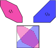
Refer to caption — Figure 1: Two polygons and the convex hull of their union

The computation of $\mvol(Q_{1},\dots,Q_{n})$ can be greatly simplified when some of the polytopes are identical, known as semi-mixed cases [35, 43]. The extreme case where all polytopes are identical, i.e., $Q_{1}=\cdots=Q_{n}$ , is known as the unmixed case which is equivalent to volume computation in the sense that $\mvol(Q,\dots,Q)=n!\vvol_{n}(Q)$ . Algorithms for calculating volume of polytopes can therefore be used in such unmixed cases. The main goal of the present contribution is to establish conditions under which mixed volume computation can be turned into unmixed cases in the same dimension. That is, we state conditions under which $\mvol(Q_{1},\dots,Q_{n})=n!\vvol_{n}(\conv(Q_{1}\cup\dots\cup Q_{n}))$ where “ $\conv$ ” denotes the operation of taking convex hull.

Example 1

In $\mathbb{R}^{2}$ , consider, the two convex polytopes (polygons)

	$\displaystyle Q_{1}$	$\displaystyle=\conv\{(1,1),(3,0),(4,0),(4,1),(3,3),(1,4),(0,4),(0,3)\}$
	$\displaystyle Q_{2}$	$\displaystyle=\conv\{(0,1),(0,0),(3,0),(4,1),(4,4),(3,4)\}$

in Fig. 1. We can verify that $\mvol(Q_{1},Q_{2})=2\vvol_{2}(\conv(Q_{1}\cup Q_{2}))=32$ . The monotonicity of mixed volume implies that $\mvol(Q_{1},Q_{2})\leq 2\vvol_{n}(\conv(Q_{1}\cup Q_{2}))$ , but the equality will not hold in general, since one side is invariant under translations of $Q_{1}$ and $Q_{2}$ while the other is not. Understanding when and why this equality would hold is our main goal. Here, turning $\mvol(Q_{1},Q_{2})$ into $2\vvol(\conv(Q_{1}\cup Q_{2}))$ is computationally beneficial since $\conv(Q_{1}\cup Q_{2})$ , having only 4 vertices, is significantly less complicated than both $Q_{1}$ and $Q_{2}$ .

We shall establish certain sufficient conditions under which $\mvol(Q_{1},\dots,Q_{n})$ exactly equals $n!\vvol_{n}(\conv(Q_{1}\cup\dots\cup Q_{n}))$ . They can be summarized into the following theorems which clearly apply to the above example. As we shall note in Remark 2, these conditions can, in principle, be checked automatically as by-products of the process of computing the volume of $\conv(Q_{1}\cup\dots\cup Q_{n})$ .

Theorem 1.1

For finite sets $S_{1},\dots,S_{n}\subset\mathbb{Q}^{n}$ , let $\tilde{S}=S_{1}\cup\cdots\cup S_{n}$ . If for every proper positive dimensional face $F$ of $\conv(\tilde{S})$ we have $F\cap S_{i}\neq\varnothing$ for each $i=1,\dots,n$ then $\mvol(\conv S_{1},\dots,\conv S_{n})=n!\vvol_{n}(\conv(\tilde{S}))$ .

Theorem 1.2

Given nonempty finite sets $S_{1},\dots,S_{n}\subset\mathbb{Q}^{n}$ , let $\tilde{S}=S_{1}\cup\cdots\cup S_{n}$ . If every positive dimensional face $F$ of $\conv(\tilde{S})$ satisfies one of the following conditions:

(A): $F\cap S_{i}\neq\varnothing$ for all $i\in\{1,\dots,n\}$ ;
(B): $F\cap S_{i}$ is a singleton for some $i\in\{1,\dots,n\}$ ;
(C): For each $i\in I:=\{i\mid F\cap S_{i}\neq\varnothing\}$ , $F\cap S_{i}$ is contained in a common coordinate subspace of dimension $|I|$ , and the projection of $F$ to this subspace is of dimension less than $|I|$ ;

then $\mvol(\conv(S_{1}),\dots,\conv(S_{n}))=n!\vvol_{n}(\conv(\tilde{S}))$ .

These theorems transform the mixed volume of $n$ polytopes into normalized volume of a single polytope in the same ambient space — the convex hull of their union. Computationally, the potential advantage is three-fold:

1.

When some of the $S_{i}$ ’s contain common points, such redundancy is removed in the union $\tilde{S}:=S_{1}\cup\cdots\cup S_{n}$ in the sense that $|\tilde{S}|<|S_{1}|+\cdots+|S_{n}|$ . Since the number of vertices plays an important role in the complexity of algorithms for manipulating polytopes, it may be much more efficient to study $\conv(\tilde{S})$ in such cases.
2.

In forming the union $\tilde{S}:=S_{1}\cup\cdots\cup S_{n}$ , certain vertices of some of the $\conv(S_{i})$ may no longer be vertices of $\conv(\tilde{S})$ and hence can be ignored in computing $n!\vvol(\conv(\tilde{S}))$ .
3.

Currently, there appear to be a greater variety of efficient algorithms for volume computation than for mixed volume computation (see [11] and [25]).

The combined effect of these computational advantages can lead to substantial reduction of computational costs for certain problems as we shall demonstrate. Moreover, the equivalence of mixed volume and normalized volume is likely to lead to alternative algorithms for approximating mixed volume since there are well-studied polynomial time algorithms for approximating volume in general.

Of course, this transformation can also be used in reverse: The volume of a single polytope could be reduced to mixed volume of several simpler polytopes which can potentially be easier to compute. Indeed, this idea was used in the author’s recent work [18] (with Robert Davis) to show that the normalized volume of a free sum of two polytopes is simply the product of their normalized volume.

Interestingly, this problem is also studied by Frédéric Bihan and Ivan Soprunov around the same time [10] from a different point of view. In particular, Theorem 1.1 turns out to be a special case of their more general results.

This paper is structured as follows: §2 shows a geometric the connection between mixed volume and volume via a simple example. §3 reviews concepts to be used. The main proofs are given in §4. They are generalized to the semi-mixed cases in §5. Their applicability are demonstrated in §6 via problems from real-world applications. §7 highlights the potentially substantial reduction in computational costs achieved by these transformations. Finally, §8 explores the implication in the polyhedral homotopy method for solving polynomial systems.

2 A geometric motivation

Before presenting the proofs, we use a simple example to show intuitively why there could be any connections between mixed volume of several polytopes and the normalized volume of the convex hull of their union at all.

Consider the simple 2-dimensional example shown in Figure 2 with

	$\displaystyle Q_{1}$	$\displaystyle=\{(0,0),(0,2),(2,0),(2,2)\}$
	$\displaystyle Q_{2}$	$\displaystyle=\{(0,0),(1,2),(2,1)\}$

which satisfies the assumptions in Theorem 1.1: all edges of $\conv(Q_{1}\cup Q_{2})$ intersect with both $Q_{1}$ and $Q_{2}$ . In Figure 2, we can easily see that the Minkowski sum $Q_{1}+Q_{2}$ contains a copy of $Q_{1}$ and a copy of $Q_{2}$ . Under the scaling of $Q_{1}\mapsto\lambda_{1}Q_{1}$ and $Q_{2}\mapsto\lambda_{2}Q_{2}$ , the area of those copies of $Q_{1}$ and $Q_{2}$ are scaled by $\lambda_{1}^{2}$ and $\lambda_{2}^{2}$ respectively. The remaining regions whose area will scale with the factor $\lambda_{1}\cdot\lambda_{2}$ are known as mixed cells. The sum of the areas of these mixed cells is exactly the mixed volume [43]. In this case, the mixed volume is 8.

We now examine the growth rate of the normalized volume $v(\lambda)=2\vvol_{2}(Q_{1}\cup\lambda Q_{2})$ as a function of the positive real scalar $\lambda$ . From Figure 3, we can see it is a piecewise function: For $\lambda\leq 1$ , $\lambda Q_{2}$ is contained in $Q_{1}$ , therefore $v(\lambda)$ remains a constant; For $1\leq\lambda\leq\frac{4}{3}$ , vertices of $\lambda Q_{2}$ start to push out of $Q_{1}$ while edges remain partially in $Q_{1}$ , and $v(\lambda)$ grows linearly; Finally, for $\lambda>\frac{4}{3}$ , an edge of $\lambda Q_{2}$ leaves $Q_{1}$ , and $v(\lambda)$ grows quadratically.

(a) For

\lambda<1

v(\lambda)

remains constant

(b) For

1\leq\lambda\leq 4/3

v(\lambda)

grows linearly

Figure 3: The growth rate of

v(\lambda)=2\vvol_{2}(Q_{1}\cup\lambda Q_{2})

for different ranges of

\lambda

Indeed, it is easy to verify that

v(\lambda)=2\vvol_{2}(\conv{Q_{1}\cup\lambda Q_{2}})=\begin{cases}8&\text{if }\lambda\leq 1\\ 8\lambda&\text{if }1<\lambda\leq\frac{4}{3}\\ 4\lambda+3\lambda^{2}&\text{if }\lambda>\frac{4}{3}.\end{cases}

That is, for any $\lambda\in[1,4/3]$ ,

v(\lambda)=2\vvol_{2}(Q_{1}\cup\lambda Q_{2})=\mvol(Q_{1},\lambda Q_{2}).

This interval $[1,4/3]$ for $\lambda$ is precisely the interval for which the pair $(Q_{1},\lambda Q_{2})$ satisfies the conditions in Theorem 1.1, i.e., all edges of $\conv(Q_{1}\cup Q_{2})$ intersect both $Q_{1}$ and $Q_{2}$ . This example also shows that the conditions required by Theorem 1.1 are not just very special configurations of two polytopes but can remain valid under a range of scaling.

A more direct connection between the normalized volume and mixed volume can be visualized through mixed cells (Figure 2). Recall that the sum of the area of the mixed cells is precisely the mixed volume. As shown in Figure 4, for $\lambda\in[1,4/3]$ , e.g. $\lambda=1.2$ (Figure 3(c)) two copies of $\conv(Q_{1}\cup\lambda Q_{2})$ can be subdivided and rearranged to form the two mixed cells of $(Q_{1},\lambda Q_{2})$ in Figure 2. Therefore, the normalized volume $2\vvol_{2}(\conv(Q_{1}\cup\lambda Q_{2}))$ is precisely the mixed volume $\mvol(Q_{1},\lambda Q_{2})$ .

The geometric observation illustrated above shows a potential connection between the mixed volume of polytopes and the volume of the convex hull of their union under the assumptions of Theorem 1.1, and this is the main motivation behind this study. However, the author was unable to generalize this to a proof. Using the theory of Bernshtein-Kushnirenko-Khovanskii bound for Laurent polynomial systems, this paper presents a purely algebraic proof.

3 Preliminaries

For a compact set $Q\subset\mathbb{R}^{n}$ , $\vvol_{n}(Q)$ denotes its standard Euclidean volume, and the quantity $n!\vvol_{n}(Q)$ is known as its normalized volume. Given a nonzero vector $\boldsymbol{\alpha}\in\mathbb{R}^{n}$ , we also define $h_{\boldsymbol{\alpha}}(Q):=\min\{\left\langle\mathbf{q},\boldsymbol{\alpha}\right\rangle\mid\mathbf{q}\in Q\}$ and $(Q)_{\boldsymbol{\alpha}}:=\{\mathbf{q}\in Q\mid\left\langle\mathbf{q},\boldsymbol{\alpha}\right\rangle=h_{\boldsymbol{\alpha}}(Q)\}$ . A convex polytope $P\subset\mathbb{R}^{n}$ is the convex hull of a finite set. A subset of the form $(P)_{\boldsymbol{\alpha}}$ is called a face of $P$ . Each face has a well defined dimension. A face of dimension 0 must be a point and is known as a vertex. Other nonempty faces are said to be positive dimensional.

The Minkowski sum of two sets $A,B\subset\mathbb{R}^{n}$ is $A+B=\{\mathbf{a}+\mathbf{b}\mid\mathbf{a}\in A,\mathbf{b}\in B\}$ . Given convex polytopes $Q_{1},\dots,Q_{n}\subset\mathbb{R}^{n}$ , the Minkowski sum $\lambda_{1}Q_{1}+\cdots+\lambda_{n}Q_{n}$ is also a convex polytope, and its volume is a homogeneous polynomial in the positive scalars $\lambda_{1},\dots,\lambda_{n}$ . In it, the coefficient¹¹ 1 An alternative definition for mixed volume is the coefficient of $\lambda_{1}\cdots\lambda_{n}$ in that polynomial divided by $n!$ . of $\lambda_{1}\cdots\lambda_{n}$ is the mixed volume [67] of $Q_{1},\dots,Q_{n}$ , denoted $\mvol(Q_{1},\dots,Q_{n})$ . Mixed volume is symmetric, additive, and nondecreasing (see §A).

Though the main results to be established are in the realm of geometry, our proofs take a decidedly algebraic approach via the theory of root counting. A Laurent monomial in $\mathbf{x}=(x_{1},\dots,x_{n})$ induced by vector $\mathbf{a}=(a_{1},\dots,a_{n})\in\mathbb{Z}^{n}$ is the formal expression $\mathbf{x}^{\mathbf{a}}=x_{1}^{a_{1}}\cdots x_{n}^{a_{n}}$ . A Laurent polynomial a linear combination of distinct Laurent monomials, i.e., an expression of the form $p=\sum_{\mathbf{a}\in S}c_{\mathbf{a}}\mathbf{x}^{\mathbf{a}}$ . The set $S\subset\mathbb{Z}^{n}$ collecting all the exponent vectors is known as the support of $p$ , denoted $\supp(p)$ , and the convex hull $\conv(S)$ is known as the Newton polytope of $p$ . For a Laurent polynomial system $P=(p_{1},\dots,p_{m})$ in $\mathbf{x}=x_{1},\dots,x_{n}$ , we define $\mathbb{V}^{*}(P):=\{\mathbf{x}\in(\mathbb{C}^{*})^{n}\mid P(\mathbf{x})=\boldsymbol{0}\}$ , and it consists of components each with a well defined dimension. Of special interest in our discussion are the components of zero dimension which are the isolated points²² 2 Here, a point $\mathbf{x}\in\mathbb{V}^{*}(P)$ is said to be isolated (a.k.a. geometrically isolated) if there is an open set in $(\mathbb{C}^{*})^{n}$ that contains $\mathbf{x}$ but does not contain any other points in $\mathbb{V}^{*}(P)$ . in $\mathbb{V}^{*}(P)$ . This subset will be denoted by $\mathbb{V}_{0}^{*}(P)$ . The proofs of our main results rely on the following important theorems.

Theorem 3.1 (Kushnirenko [52])

For a Laurent polynomial system $P=(p_{1},\dots,p_{n})$ in $\mathbf{x}=(x_{1},\dots,x_{n})$ with identical support, $S=\supp(p_{i})$ for $i=1,\dots,n$ , we have $|\mathbb{V}_{0}^{*}(P)|\leq n!\vvol_{n}(\conv(S))$ .

Theorem 3.2 (Bernshtein’s First Theorem [8])

For a Laurent polynomial system $P=(p_{1},\dots,p_{n})$ in $\mathbf{x}=(x_{1},\dots,x_{n})$ (with potentially different supports), $|\mathbb{V}_{0}^{*}(P)|\leq\mvol(\conv(\supp(p_{1})),\dots,\conv(\supp(p_{n})))$ .

In [12], this upper bound was nicknamed the BKK bound after the works of Bernshtein [8, 9], Kushnirenko [52], and Khovanskii [47]. The condition under which the BKK bound is exact (counting multiplicity) is stated in terms of “initial systems”: For a Laurent polynomial $p=\sum_{\mathbf{a}\in S}c_{\mathbf{a}}\mathbf{x}^{\mathbf{a}}$ in $\mathbf{x}=(x_{1},\dots,x_{n})$ and a nonzero vector $\boldsymbol{\alpha}\in\mathbb{R}^{n}$ , $\init_{\boldsymbol{\alpha}}(p):=\sum_{\mathbf{a}\in(S)_{\boldsymbol{\alpha}}}c_{\mathbf{a}}\mathbf{x}^{\mathbf{a}}$ . For a Laurent polynomial system $P=(p_{1},\dots,p_{m})$ , the initial system of $P$ with respect to $\boldsymbol{\alpha}$ is $\init_{\boldsymbol{\alpha}}(P):=(\init_{\boldsymbol{\alpha}}(p_{1}),\dots,\init_{\boldsymbol{\alpha}}(p_{m}))$ .

Theorem 3.3 (Bernshtein’s Second Theorem [8])

For a Laurent polynomial system $P=(p_{1},\dots,p_{n})$ in $\mathbf{x}=(x_{1},\dots,x_{n})$ with supports $S_{1}=\supp(p_{1}),\dots,S_{n}=\supp(p_{n})$ , if for all $\boldsymbol{\alpha}\in\mathbb{R}^{n}\setminus\{\boldsymbol{0}\}$ , $\init_{\boldsymbol{\alpha}}(P)$ has no zeros in $(\mathbb{C}^{*})^{n}$ , then all zeros of $P$ in $(\mathbb{C}^{*})^{n}$ are isolated, and, counting multiplicity, the total number of zeros is exactly $\mvol(\conv(S_{1}),\dots,\conv(S_{n}))$ .

Remark 1

An important fact is that the BKK bound is always attainable. That is, fixing the supports of $P$ , there is always some choice of the coefficients for which all points in $\mathbb{V}_{0}^{*}(P)$ are simple (of multiplicity one), and $|\mathbb{V}_{0}^{*}(P)|=\mvol(\conv(\supp(p_{1})),\dots,\conv(\supp(p_{n})))$ . In this case, $P$ is said to be in general position (with respect to the supports). Indeed, such choices form a nonempty Zariski open set in the coefficient space [12, 37, 42, 58, 70, 71].

4 Proofs of the main results

The proofs of the main theorems all rely on the theory of BKK bound. Given a system of $n$ Laurent polynomial systems $P=(p_{1},\dots,p_{n})$ in $n$ variables with supports $S_{1},\dots,S_{n}$ and Newton polytopes $Q_{i}=\conv(S_{i})$ . If $P$ is in general position (Remark 1) the $\mathbb{C}^{*}$ -root count is exactly the mixed volume $\mvol(Q_{1},\dots,Q_{n})$ . For a nonsingular square matrix $A$ , the systems $A\cdot P$ and $P$ have the exact same set of $\mathbb{C}^{*}$ -roots. Moreover, if $A$ is chosen generically, $\supp(A\cdot P)$ is exactly the union of $S_{1},\dots,S_{n}$ . Therefore, we have

\mvol(Q_{1},\dots,Q_{n})=|\mathbb{V}_{0}^{*}(P)|=|\mathbb{V}_{0}^{*}(A\cdot P)|\leq n!\vvol(\conv(S_{1}\cup\dots\cup S_{n})).

In general, we may not have the equality because $A\cdot P$ itself may not be in general position as a member of the much larger family of Laurent polynomial systems with Newton polytopes $\conv(S_{1}\cup\dots\cup S_{n})$ . We establish the equality by showing under certain conditions, if $P$ is general position, then $A\cdot P$ is also in general position.

The proofs make repeated use of a simple geometric observation illustrated in Fig. 5. We state it as a lemma for later reference:

Lemma 1

For $n$ nonempty sets $S_{1},\dots,S_{n}\subset\mathbb{Q}^{n}$ , let $F$ be a proper face of $\conv(S_{1}\cup\cdots\cup S_{n})$ and $\boldsymbol{\alpha}$ be its inner normal. For each $i$ such that $F\cap S_{i}\neq\varnothing$ , $F\cap S_{i}=(S_{i})_{\boldsymbol{\alpha}}$ .

Proof

Fix an $i\in\{1,\dots,n\}$ such that $F\cap S_{i}\neq\varnothing$ . If we let $h=h_{\boldsymbol{\alpha}}(\conv(S_{1}\cup\cdots\cup S_{n}))$ then for any $\mathbf{x}\in F\cap S_{i}$ , $\left\langle\mathbf{x},\boldsymbol{\alpha}\right\rangle=h$ while for any $\mathbf{y}\in S_{i}\setminus F\subseteq\conv(S_{1}\cup\cdots\cup S_{n})\setminus F$ we have $\left\langle\mathbf{y},\boldsymbol{\alpha}\right\rangle>h$ . Therefore $F\cap S_{i}=(S_{i})_{\boldsymbol{\alpha}}$ . ∎

With this lemma, we restate and prove the two main theorems listed earlier.

See 1.1

Proof

We shall first prove the cases where $S_{i}\subset\mathbb{Z}^{n}$ for $i=1,\dots,n$ . Let $P=(p_{1},\dots,p_{n})$ be a Laurent polynomial system in $\mathbf{x}=(x_{1},\dots,x_{n})$ such that $\supp(p_{i})=S_{i}$ for each $i$ . That is, $p_{i}(\mathbf{x})=\sum_{\mathbf{a}\in S_{i}}c_{i,\mathbf{a}}\mathbf{x}^{\mathbf{a}}$ . By Theorem 3.2, Theorem 3.3, and Remark 1, there exists a choice of the coefficients $\{c_{i,\mathbf{a}}\mid\mathbf{a}\in S_{i},i=1,\dots,n\}$ such that $P$ is in general position, i.e., all points in $\mathbb{V}_{0}^{*}(P)$ are simple and

|\mathbb{V}_{0}^{*}(P)|=\mvol(\,\conv(S_{1}),\dots,\conv(S_{n})\,).

(1)

Now, consider a randomization [76] $A\cdot P$ of $P$ induced by a nonsingular $n\times n$ complex matrix $A=[a_{ij}]$ :

A\cdot P:=\begin{bmatrix}a_{11}&\cdots&a_{1n}\\ \vdots&\ddots&\vdots\\ a_{n1}&\cdots&a_{nn}\end{bmatrix}\begin{bmatrix}p_{1}\\ \vdots\\ p_{n}\end{bmatrix}=\begin{bmatrix}a_{11}p_{1}+\cdots+a_{1n}p_{n}\\ \vdots\\ a_{n1}p_{1}+\cdots+a_{nn}p_{n}\end{bmatrix}.

(2)

Since $A$ is nonsingular, $(A\cdot P)(\mathbf{x})=A\cdot(P(\mathbf{x}))=\boldsymbol{0}$ if and only if $P(\mathbf{x})=\boldsymbol{0}$ . Therefore, $A\cdot P$ and $P$ have the same zeros. In particular, $\mathbb{V}_{0}^{*}(A\cdot P)=\mathbb{V}_{0}^{*}(P)$ , and all of its points are simple.

With the coefficients of $P$ already fixed, we assume entries of $A$ are chosen so that there are no cancellations of terms in $A\cdot P$ , then it is easy to verify that the supports of the Laurent polynomials in $A\cdot P$ are identical which is

\supp(a_{i1}p_{1}+\cdots+a_{in}p_{n})=S_{1}\cup\cdots\cup S_{n}=:\tilde{S}

for each $i=1,\dots,n$ . By Kushnirenko’s Theorem (Theorem 3.1),

|\mathbb{V}_{0}^{*}(A\cdot P)|\leq n!\vvol_{n}(\conv(\tilde{S})).

(3)

Theorem 3.3 and Remark 1 states that the equality holds as long as for any nonzero vector $\boldsymbol{\alpha}\in\mathbb{R}^{n}$ , the initial system $\init_{\boldsymbol{\alpha}}(A\cdot P)$ has no zero in $(\mathbb{C}^{*})^{n}$ . Let $F:=(\conv(\tilde{S}))_{\boldsymbol{\alpha}}$ . If $F$ is a vertex, i.e., $F=\{\mathbf{a}\}$ for some $\mathbf{a}\in\tilde{S}$ , then each component of $\init_{\boldsymbol{\alpha}}(A\cdot P)$ has only one term: the term involving $\mathbf{x}^{\mathbf{a}}$ . Therefore $\init_{\boldsymbol{\alpha}}(A\cdot P)$ has no zero in $(\mathbb{C}^{*})^{n}$ . Otherwise, $F$ is positive dimensional and hence, by assumption, $F$ intersects each $S_{i}$ . By Lemma 1, $F\cap S_{i}=(S_{i})_{\boldsymbol{\alpha}}$ for each $i=1,\dots,n$ . Therefore,

\init_{\boldsymbol{\alpha}}(A\cdot P)=\begin{bmatrix}\displaystyle\sum_{i=1}^{n}a_{1i}\sum_{\mathbf{a}\in F\cap S_{i}}c_{i,\mathbf{a}}\mathbf{x}^{\mathbf{a}}\\ \vdots\\ \displaystyle\sum_{i=1}^{n}a_{ni}\sum_{\mathbf{a}\in F\cap S_{i}}c_{i,\mathbf{a}}\mathbf{x}^{\mathbf{a}}\\ \end{bmatrix}=A\cdot\begin{bmatrix}\displaystyle\sum_{\mathbf{a}\in F\cap S_{1}}c_{1,\mathbf{a}}\mathbf{x}^{\mathbf{a}}\\ \vdots\\ \displaystyle\sum_{\mathbf{a}\in F\cap S_{n}}c_{n,\mathbf{a}}\mathbf{x}^{\mathbf{a}}\\ \end{bmatrix}=A\cdot\begin{bmatrix}\init_{\boldsymbol{\alpha}}(p_{1})\\ \vdots\\ \init_{\boldsymbol{\alpha}}(p_{n})\end{bmatrix}.

(4)

That is, $\init_{\boldsymbol{\alpha}}(A\cdot P)=A\cdot\init_{\boldsymbol{\alpha}}(P)$ . Recall that $A$ is nonsingular, so $\init_{\boldsymbol{\alpha}}(A\cdot P)=\boldsymbol{0}$ if and only if $\init_{\boldsymbol{\alpha}}(P)=\boldsymbol{0}$ . But $P$ is in general position, so

\mathbb{V}^{*}(\init_{\boldsymbol{\alpha}}(A\cdot P))=\mathbb{V}^{*}(\init_{\boldsymbol{\alpha}}(P))=\varnothing.

Therefore for all nonzero vector $\boldsymbol{\alpha}\in\mathbb{R}^{n}$ , $\init_{\boldsymbol{\alpha}}(A\cdot P)$ has no zero in $(\mathbb{C}^{*})^{n}$ . Recall that all points in $\mathbb{V}_{0}^{*}(A\cdot P)$ are simple, so by Bernshtein’s Second Theorem (Theorem 3.3), $|\mathbb{V}_{0}^{*}(A\cdot P)|=n!\vvol(\conv(\tilde{S}))$ , and consequently

\mvol(\conv S_{1},\dots,\conv S_{n})=|\mathbb{V}_{0}^{*}(P)|=|\mathbb{V}_{0}^{*}(A\cdot P)|=n!\vvol(\conv(\tilde{S})).

Since both sides of this equality are homogeneous of degree $n$ in a uniform positive scaling, this result directly extend to cases with $S_{i}\subset\mathbb{Q}^{n}$ . ∎

See 1.2

Proof

We shall reuse the previous constructions: Let the Laurent polynomial system $P$ , nonsingular matrix $A$ , and the randomization $A\cdot P$ be those defined in the previous proof. Then $\supp(A\cdot P)=(\tilde{S},\dots,\tilde{S})$ and

\mvol(\conv(S_{1}),\dots,\conv(S_{n}))=|\mathbb{V}^{*}_{0}(P)|=|\mathbb{V}^{*}_{0}(A\cdot P)|\leq n!\vvol(\conv(\tilde{S})).

The goal is still to establish the equality by showing for any nonzero vector $\boldsymbol{\alpha}\in\mathbb{R}^{n}$ , $\init_{\boldsymbol{\alpha}}(A\cdot P)$ has no zero in $(\mathbb{C}^{*})^{n}$ under the above assumptions. Let $F=(\conv(\tilde{S}))_{\boldsymbol{\alpha}}$ . If $F$ is a vertex or satisfies condition (A), the proof for Theorem 1.1 has already shown that $\mathbb{V}^{*}(\init_{\boldsymbol{\alpha}}(A\cdot P))=\varnothing$ .

To study the remaining possibilities, we may assume $F$ is positive dimensional and $F\cap S_{j}=\varnothing$ for some $j$ . Let $I:=\{i\in\{1,\dots,n\}\mid F\cap S_{i}\neq\varnothing\}=\{i_{1},\dots,i_{m}\}$ with $m=|I|<n$ . Then by Lemma 1, $F\cap S_{i}=(S_{i})_{\boldsymbol{\alpha}}$ for each $i\in I$ . Hence

\displaystyle\init_{\boldsymbol{\alpha}}(A\cdot P)=\begin{bmatrix}\displaystyle\sum_{i\in I}a_{1i}\sum_{\mathbf{a}\in F\cap S_{i}}c_{i,\mathbf{a}}\mathbf{x}^{\mathbf{a}}\\ \vdots\\ \displaystyle\sum_{i\in I}a_{ni}\sum_{\mathbf{a}\in F\cap S_{i}}c_{i,\mathbf{a}}\mathbf{x}^{\mathbf{a}}\end{bmatrix}=\begin{bmatrix}\displaystyle\sum_{i\in I}a_{1i}\init_{\boldsymbol{\alpha}}(p_{i})\\ \vdots\\ \displaystyle\sum_{i\in I}a_{ni}\init_{\boldsymbol{\alpha}}(p_{i})\end{bmatrix}=A_{I}\cdot\init_{\boldsymbol{\alpha}}(P_{I})

where $A_{I}$ is the matrix whose columns consists of the $i$ -th columns of $A$ for $i\in I$ and $P_{I}$ is the Laurent polynomial system (as a column vector) whose components are $p_{i}$ for $i\in I$ . Since $A$ is assumed to be nonsingular, $A_{I}$ has rank $|I|$ . Therefore $\boldsymbol{0}=\init_{\boldsymbol{\alpha}}(A\cdot P)=A_{I}\cdot\init_{\boldsymbol{\alpha}}(P_{I})$ if and only if $\init_{\boldsymbol{\alpha}}(P_{I})=\boldsymbol{0}$ .

Case (B) Assume $F$ satisfies condition (B), then there is at least one $i_{1}\in I$ for which $F\cap S_{i_{1}}=(S_{i_{1}})_{\boldsymbol{\alpha}}$ is a singleton, i.e., $F\cap S_{i_{1}}=\{\mathbf{a}\}$ for some $\mathbf{a}\in S_{i_{1}}$ . Therefore, $\init_{\boldsymbol{\alpha}}(p_{i_{1}})=c_{i_{1},\mathbf{a}}\mathbf{x}^{\mathbf{a}}$ where $c_{i_{1},\mathbf{a}}\neq 0$ , and hence it has no zero in $(\mathbb{C}^{*})^{n}$ . Consequently,

\mathbb{V}^{*}(\init_{\boldsymbol{\alpha}}(A\cdot P))=\mathbb{V}^{*}(A_{I}\cdot\init_{\boldsymbol{\alpha}}(P_{I}))=\mathbb{V}^{*}(\init_{\boldsymbol{\alpha}}(P_{I}))\subseteq\mathbb{V}^{*}(\init_{\boldsymbol{\alpha}}(p_{i_{1}}))=\varnothing.

That is, $\mathbb{V}^{*}(\init_{\boldsymbol{\alpha}}(A\cdot P))=\varnothing$ .

Case (C) Finally, assume $F$ satisfies condition (C). Then $\supp(\init_{\boldsymbol{\alpha}}(P_{I}))=(F\cap S_{i_{1}},\dots,F\cap S_{i_{m}})$ lie in a common coordinate subspace of dimension $m=|I|$ . Let $j_{1},\dots,j_{m}$ be the indices so that $\mathbf{e}_{j_{1}},\dots,\mathbf{e}_{j_{m}}$ form a basis for this coordinate subspace. Then $\init_{\boldsymbol{\alpha}}(P_{I})$ only involves $m$ of the $n$ variables $x_{j_{1}},\dots,x_{j_{m}}$ . To emphasize this, we shall write it as $P_{F}=P_{F}(x_{j_{1}},\dots,x_{j_{m}})$ , and it is a square system of $m$ equations in $m$ variables. Let $\pi:\mathbb{R}^{n}\to\mathbb{R}^{m}$ be the projection into the common coordinate subspace, then $\supp(P_{F})=(\pi(F\cap S_{i_{1}}),\dots,\pi(F\cap S_{i_{m}}))$ . It is also assumed that the projection $\pi(F)$ is of dimension less than $m$ . Then the supports of $P_{F}$ lie in an affine subspace of dimension less than $m$ . Consequently

\mvol(\supp(P_{F}))=\mvol(\pi(F\cap S_{i_{1}}),\dots,\pi(F\cap S_{i_{m}}))=0.

(5)

Notice that the coefficients of $P_{F}$ is a subset of the coefficients of the original system $P=(p_{1},\dots,p_{n})$ . So there is a nonempty Zariski open set $C_{F}$ among the choices of coefficients for $P$ for which $P_{F}$ is also in general position.

Since $\conv(\tilde{S})$ has finitely many faces and in Zariski topology, any two nonempty open set must intersect, without loss of generality, we may assume the coefficients for $P$ is chosen so that $P_{F}$ is in general position for all proper positive dimensional faces $F$ . Then by (5), $\mathbb{V}^{*}(P_{F})=\mathbb{V}^{*}_{0}(P_{F})=\varnothing$ . Recall that $P_{F}(x_{j_{1}},\dots,x_{j_{m}})$ is simply $\init_{\boldsymbol{\alpha}}(P_{I})$ but ignoring the $n-m$ variables that do not actually appear. So for any $\mathbf{x}=(x_{1},\dots,x_{n})\in\mathbb{V}^{*}(\init_{\boldsymbol{\alpha}}(P_{I}))$ , we must have $(x_{j_{1}},\dots,x_{j_{m}})\in\mathbb{V}^{*}(P_{F})=\varnothing$ . Therefore $\mathbb{V}^{*}(\init_{\boldsymbol{\alpha}}(P_{I}))=\varnothing$ which implies $\mathbb{V}^{*}(\init_{\boldsymbol{\alpha}}(A\cdot P))=\mathbb{V}^{*}(\init_{\boldsymbol{\alpha}}(P_{I}))=\varnothing$ .

We can now conclude that under the assumptions (A),(B), and (C) for any nonzero vector $\boldsymbol{\alpha}\in\mathbb{R}^{n}$ , $\init_{\boldsymbol{\alpha}}(A\cdot P)$ has no zero in $(\mathbb{C}^{*})^{n}$ . Then by Bernshtein’s Second Theorem (Theorem 3.3) $|\mathbb{V}_{0}^{*}(A\cdot P)|=n!\vvol(\conv(\tilde{S}))$ , and consequently

\mvol(\conv S_{1},\dots,\conv S_{n})=|\mathbb{V}_{0}^{*}(P)|=|\mathbb{V}_{0}^{*}(A\cdot P)|=n!\vvol(\conv(\tilde{S})).

As in the previous case, since both sides of this equality are homogeneous of degree $n$ in a uniform positive scaling, this result directly extend to cases with $S_{i}\subset\mathbb{Q}^{n}$ . ∎

The above proofs also produced a byproduct that is potentially useful in numerical methods for solving system of Laurent polynomials:

Proposition 1

Let $P=(p_{1},\dots,p_{n})$ be a Laurent polynomial system in general position that satisfies the conditions in Theorem 1.1 or Theorem 1.2. For a generic square complex matrix $A$ , the system $A\cdot P$ is also in general position.

This property is particularly important in the numerical homotopy continuation methods for solving Laurent polynomial systems and is explored in § 8.

Remark 2 (Automatic verification during volume computation)

The conditions for the two theorems proved above involve how faces of $\conv(\tilde{S})=\conv(S_{1}\cup\cdots S_{n})$ intersect or fail to intersect each $S_{i}$ . These, in principle, can be verified automatically as by-products from the process of computing the volume of $\conv(\tilde{S})$ using a certain kind of subdivision algorithm: If the polytope is represented as the convex hull of a set of points, a particularly simple procedure for constructing a subdivision for the convex polytope $\conv(\tilde{S})$ starts with the enumeration of all its facets. Then the collection of all the pyramids formed by the facets and a fixed interior point will be a subdivision of the polytope. With this construction, since the set of all facets is already generated, the conditions of the above theorems can be checked easily.

5 Turning mixed volume into semi-mixed types

With minor modifications, the above proofs generalize directly to cases where union is taken over only a subset of the polytopes whereby transforming the mixed volume into semi-mixed types even when the Newton polytopes are all distinct. This transformation will be particularly beneficial when a subset of polytopes have nearly identical (but still different) set of vertices (e.g. the Tensor Eigenvalue Problem to be discussed in §6.4. In such cases, taking the union over these similar subset of polytopes will not only simplify the geometric information but also allow one to use the much more efficient algorithms for mixed volume computation of semi-mixed types [24, 35].

Corollary 1 (Semi-mixed version of Theorem 1.1)

Given nonempty finite sets $S_{i,j}\linebreak\subset\mathbb{Q}^{n}$ for $i=1,\dots,m$ and $j=1,\dots,k_{i}$ with $k_{i}\in\mathbb{Z}^{+}$ and $k_{1}+\cdots+k_{m}=n$ , let $Q_{i,j}=\conv(S_{i,j})$ , $\tilde{S}_{i}=\bigcup_{j=1}^{k_{i}}S_{i,j}$ , and $\tilde{Q}_{i}=\conv(\tilde{S}_{i})$ . If for each $i$ , every positive dimensional face of $\tilde{Q}_{i}$ that intersect $S_{i,j}$ for some $j$ on at least two points must intersect all $S_{i,1},\dots,S_{i,k_{i}}$ , then

\mvol(Q_{1,1},\dots,Q_{m,k_{m}})=\mvol(\;\underbrace{\tilde{Q}_{1},\dots,\tilde{Q}_{1}}_{k_{1}}\,,\;\dots,\;\underbrace{\tilde{Q}_{m},\dots,\tilde{Q}_{m}}_{k_{m}}\;).

Proof

Let $P=(p_{ij})_{i=1,\dots,m,j=1\dots,k_{i}}$ be a system of Laurent polynomials in $\mathbf{x}=(x_{1},\dots,x_{n})$ with $p_{ij}(\mathbf{x})=\sum_{\mathbf{a}\in S_{ij}}c_{i,j,\mathbf{a}}\mathbf{x}^{\mathbf{a}}$ . Also define $P_{i}=(p_{i1},\dots,p_{ik_{i}})$ for each $i=1,\dots,m$ . We further assume the coefficients are chosen so that $P$ is in general position. By Bernshtein’s First Theorem (Theorem 3.2),

|\mathbb{V}_{0}^{*}(P)|=\mvol(Q_{1,1},\dots,Q_{m,k_{m}}).

Consider the randomization $A\cdot P$ of $P$ induced by a nonsingular $n\times n$ block matrix

A:=\left[\begin{smallmatrix}A_{1}&&&\\ &A_{2}&&\\ &&\ddots&\\ &&&A_{m}\end{smallmatrix}\right]

where each $A_{i}=[a^{(i)}_{j,k}]$ is a nonsingular $k_{i}\times k_{i}$ matrix. Since $A$ is nonsingular, $P(\mathbf{x})=\boldsymbol{0}$ if and only if $(A\cdot P)(\mathbf{x})=A\cdot(P(\mathbf{x}))=\boldsymbol{0}$ . So $\mathbb{V}_{0}^{*}(P)=\mathbb{V}_{0}^{*}(A\cdot P)$ .

As in the proof of Theorem 1.1, we further assume the entries of $A_{i}$ for $i=1,\dots,m$ are chosen so that there are no cancellations of terms in $A\cdot P$ . Then it is easy to verify that $A\cdot P$ is a semi-mixed system in the sense that among its supports each $\tilde{S}_{i}$ appear $k_{i}$ times. That is,

\supp(A\cdot P)=(\;\underbrace{\tilde{S}_{1},\dots,\tilde{S}_{1}}_{k_{1}}\,,\;\dots,\;\underbrace{\tilde{S}_{m},\dots,\tilde{S}_{m}}_{k_{m}}\;).

By Bernshtein’s First Theorem (Theorem 3.2),

|\mathbb{V}_{0}^{*}(A\cdot P)|\leq\mvol(\;\underbrace{\tilde{Q}_{1},\dots,\tilde{Q}_{1}}_{k_{1}}\,,\;\dots,\;\underbrace{\tilde{Q}_{m},\dots,\tilde{Q}_{m}}_{k_{m}}\;).

We shall establish the equality by examining the initial systems of $A\cdot P$ . For a nonzero vector $\boldsymbol{\alpha}\in\mathbb{R}^{n}$ , let $F_{i}=(\tilde{Q}_{i})_{\boldsymbol{\alpha}}$ for $i=1,\dots,m$ . We consider the following cases:

First, if $F_{i}$ is a vertex for some $i$ , then each Laurent polynomial in $\init_{\boldsymbol{\alpha}}(A_{i}\cdot P_{i})$ would have only one term, and hence $\mathbb{V}^{*}(\init_{\boldsymbol{\alpha}}(A_{i}\cdot P_{i}))=\varnothing$ . But

\init_{\boldsymbol{\alpha}}(A\cdot P)=\begin{bmatrix}\init_{\boldsymbol{\alpha}}(A_{1}\cdot P_{1})\\ \vdots\\ \init_{\boldsymbol{\alpha}}(A_{m}\cdot P_{m})\end{bmatrix},

So $\mathbb{V}^{*}(\init_{\boldsymbol{\alpha}}(A\cdot P))$ , being a subset of $\mathbb{V}^{*}(\init_{\boldsymbol{\alpha}}(A_{i}\cdot P_{i}))$ , must also be empty.

Now suppose $F_{1},\dots,F_{m}$ are all positive dimensional. We shall fix an $i\in\{1,\dots,m\}$ , and let $I_{i}=\{j\in\{1,\dots,k_{i}\}\mid F_{i}\cap S_{i,j}\neq\varnothing\}$ which must be nonempty. Then by Lemma 1,

\init_{\boldsymbol{\alpha}}(A_{i}\cdot P_{i})=\begin{bmatrix}\displaystyle\sum_{j=1}^{k_{i}}a^{(i)}_{1,j}\sum_{\mathbf{a}\in F_{i}\cap S_{i,j}}c_{i,j,\mathbf{a}}\mathbf{x}^{\mathbf{a}}\\ \vdots\\ \displaystyle\sum_{j=1}^{k_{i}}a^{(i)}_{k_{i},j}\sum_{\mathbf{a}\in F_{i}\cap S_{i,j}}c_{i,j,\mathbf{a}}\mathbf{x}^{\mathbf{a}}\end{bmatrix}=A_{I_{i}}\begin{bmatrix}\displaystyle\sum_{\mathbf{a}\in(F\cap S_{i,j})}c_{i,j,\mathbf{a}}\mathbf{x}^{\mathbf{a}}\end{bmatrix}_{j\in I_{i}}

(6)

where $A_{I_{i}}$ is the matrix containing columns of $A_{i}$ indexed by $I_{i}$ which is of rank $|I_{i}|\leq k_{i}$ . Its kernel must be $\{\boldsymbol{0}\}$ , so $\init_{\boldsymbol{\alpha}}(A_{i}\cdot P_{i})=\boldsymbol{0}$ if and only if $\sum_{\mathbf{a}\in(F\cap S_{i,j})}c_{i,j,\mathbf{a}}\mathbf{x}^{\mathbf{a}}=0$ for each $j\in I_{i}$ .

If $|F\cap S_{i,j}|=1$ for all $j\in I_{i}$ , then each of the above Laurent polynomials on the right hand side has only one term and hence no zeros in $(\mathbb{C}^{*})^{n}$ . That is, $\mathbb{V}^{*}(\init_{\boldsymbol{\alpha}}(A_{i}\cdot P_{i}))=\varnothing$ . Consequently $\mathbb{V}^{*}(\init_{\boldsymbol{\alpha}}(A\cdot P))$ , being a subset of $\mathbb{V}^{*}(\init_{\boldsymbol{\alpha}}(A_{i}\cdot P_{i}))$ must also be empty.

Now suppose for each $i=1,\dots,m$ , $|F_{i}\cap S_{i,j}|>1$ for at least one $j\in I_{i}$ , then by assumption each $F_{i}$ must intersects each of the supports $S_{i,1},\dots,S_{i,k_{i}}$ . So $I_{i}=\{1,\dots,k_{i}\}$ for each $i$ and hence $\init_{\boldsymbol{\alpha}}(A\cdot P)=A\cdot\init_{\boldsymbol{\alpha}}(P)$ . Recall that $A$ is assumed to be nonsingular, so $\init_{\boldsymbol{\alpha}}(A\cdot P)=\boldsymbol{0}$ if and only if $\init_{\boldsymbol{\alpha}}(P)=\boldsymbol{0}$ . But $P$ is assumed to be in general position, so $\mathbb{V}^{*}(\init_{\boldsymbol{\alpha}}(A\cdot P))=\mathbb{V}^{*}(\init_{\boldsymbol{\alpha}}(P))=\varnothing$ .

The above cases have shown that for all nonzero vector $\boldsymbol{\alpha}\in\mathbb{R}^{n}$ , $\mathbb{V}^{*}(\init_{\boldsymbol{\alpha}}(A\cdot P))=\varnothing$ . Then by Bernshtein’s Second Theorem (Theorem 3.3),

\mvol(Q_{1,1},\dots,Q_{m,k_{m}})=|\mathbb{V}_{0}^{*}(P)|=|\mathbb{V}_{0}^{*}(A\cdot P)|=\mvol(\underbrace{\tilde{Q}_{1},\dots,\tilde{Q}_{1}}_{k_{1}},\dots,\underbrace{\tilde{Q}_{m},\dots,\tilde{Q}_{m}}_{k_{m}}).

Since both sides of the equation are homogeneous of degree $k_{1}+\cdots+k_{m}=n$ in any positive uniform scaling of all the polytopes, this result extends directly to cases where each $S_{i,j}\subset\mathbb{Q}^{n}$ . ∎

6 Case studies

In this section, we apply the theorems proved above to concrete problems from real-world applications to reduce the mixed volume computation into the unmixed cases (volume computation) or semi-mixed cases.

6.1 Synchronization for coupled oscillators on cycle graphs

The spontaneous synchronization in networks of interconnected oscillators is a ubiquitous phenomenon that has been discovered and studied in a wide range of scientific disciplines including physics, biology, chemistry, and engineering [1, 31]. Here, as a case study, we focus on a classic model proposed by Y. Kuramoto [51]. For a network of $N=n+1$ oscillators, labeled as $0,\dots,n$ , one basic model for describing the behavior of the oscillators is the system of differential equations

\frac{d\theta_{i}}{dt}=\omega_{i}-\sum_{j=0}^{n}a_{i,j}\sin(\theta_{i}-\theta_{j})\quad\text{ for }i=0,\dots,n

(7)

where each $\omega_{i}$ is the natural frequency of the $i$ -th oscillator, each $a_{i,j}$ describes the coupling strength between the $i$ -th and $j$ -th oscillator (how strongly they influence each other), and each $\theta_{i}=\theta_{i}(t)$ is the angle of the $i$ -th oscillator. This is a mathematical representation of the tug of war between the oscillators’ tendency to oscillate in their own natural frequencies and the influence of their connected neighbors. “Synchronization” occurs when these two forces reach an equilibrium for each of the oscillators: A configuration $\boldsymbol{\theta}=(\theta_{0},\dots,\theta_{n})\in\mathbb{R}^{N}$ is said to be in synchronization³³ 3 There are several related concepts of “synchronization” in this context, which are listed in [31]. Here we only study a version of the so called frequency synchronization, a.k.a. frequency critical points. In the general context such points are characterized by all $\frac{d\theta_{i}}{dt}$ converging to a common value (not necessarily zero). However, after switching to a rotational frame of reference, it is equivalent to requiring $\frac{d\theta_{i}}{dt}=0$ for $i=0,\dots,n$ . if $\frac{d\theta_{i}}{dt}=0$ for $i=0,\dots,n$ at $\boldsymbol{\theta}$ , i.e.,

\omega_{i}-\sum_{j=0}^{n}a_{i,j}\sin(\theta_{i}-\theta_{j})=0\quad\text{ for }i=0,\dots,n

(8)

which will be referred to as the synchronization system in our discussion. The behavior of the synchronization solutions is completely understood in cases where the underlying network forms a tree [28]. Here we shall study the simplest cases beyond trees — cycle graphs. That is, we assume for each $0<i<n$ the $i$ -th node is directly connected to two nodes: $i+1$ and $i-1$ , and node 0 is directly connected to node $n$ . With the notation $i^{+}=(i+1)\mod N$ and $i^{-}=(i-1)\mod N$ , the above system can be written as

\omega_{i}-\sum_{j\in\{i^{+},i^{-}\}}a_{i,j}\sin(\theta_{i}-\theta_{j})=0\quad\text{ for }i=0,\dots,n

(9)

Note that the solutions to (8) has an inherent degree of freedom in the sense that if $(\theta_{0},\dots,\theta_{n})$ is a solution, so is $(\theta_{0}+t,\dots,\theta_{n}+t)$ for any $t$ . It is therefore a common practice to fix $\theta_{0}=0$ and remove the first equation from the system, leaving us $n=N-1$ nonlinear equations in the $n$ angles $\theta_{1},\dots,\theta_{n}$ . Using the transformation proposed in [26], we shall turn the above system into a Laurent polynomial system to which we can apply Theorem 1.2. First, using the identity $\sin(\theta_{i}-\theta_{j})=\frac{1}{2\mathbf{i}}(e^{\mathbf{i}(\theta_{i}-\theta_{j})}-e^{-\mathbf{i}(\theta_{i}-\theta_{j})})$ (9) can be transformed into

\omega_{i}-\sum_{j\in\{i^{+},i^{-}\}}\frac{a_{i,j}}{2\mathbf{i}}(e^{\mathbf{i}\theta_{i}}e^{-\mathbf{i}\theta_{j}}-e^{-\mathbf{i}\theta_{i}}e^{\mathbf{i}\theta_{j}})=0\quad\text{ for }i=1,\dots,n.

(10)

With the substitution $x_{i}:=e^{\mathbf{i}\theta_{i}}$ for $i=1,\dots,n$ , we obtain the Laurent polynomial system

\omega_{i}-\sum_{j\in\{i^{+},i^{-}\}}a_{i,j}^{\prime}(x_{i}x_{j}^{-1}-x_{j}x_{i}^{-1})=0\quad\text{ for }i=1,\dots,n

(11)

where $a_{i,j}^{\prime}=\frac{a_{i,j}}{2\mathbf{i}}$ and $x_{0}=1$ is a constant. Clearly, real solutions of (9) are represented by $\mathbb{C}^{*}$ -solutions of (11). We are interested in computing the BKK bound of this Laurent polynomial system. By applying Theorem 1.2, this can be done via volume computation which is potentially easier to compute.

Proposition 2

Let $S_{1},\dots,S_{n}$ be the supports of (11), then

\mvol(\conv(S_{1}),\dots,\conv(S_{n}))=n!\vvol_{n}(\conv(S_{1}\cup\cdots\cup S_{n})).

Proof

It is easy to verify that for each $i=1,\dots,n$ ,

S_{i}=\{\boldsymbol{0},\mathbf{e}_{i}-\mathbf{e}_{i^{+}},\mathbf{e}_{i^{+}}-\mathbf{e}_{i},\mathbf{e}_{i}-\mathbf{e}_{i^{-}},\mathbf{e}_{i^{-}}-\mathbf{e}_{i},\}

where $\mathbf{e}_{0}:=\boldsymbol{0}$ and $\mathbf{e}_{1},\dots,\mathbf{e}_{n}$ are the standard basis vectors for $\mathbb{R}^{n}$ . Let $F$ be a positive dimensional face of $\tilde{Q}=\conv(S_{1}\cup\cdots\cup S_{n})$ , $\boldsymbol{\alpha}$ be its inner normal, and $h=h_{\boldsymbol{\alpha}}(\tilde{Q})$ .

First, if $h=0$ then $\boldsymbol{0}\in F$ since $\left\langle\boldsymbol{0},\boldsymbol{\alpha}\right\rangle=0=h$ . But $\boldsymbol{0}\in S_{j}$ for each $j=1,\dots,n$ . So $F$ intersects all the supports $S_{1},\dots,S_{n}$ .

Now assume $h\neq 0$ . Since $\boldsymbol{0}\in\tilde{Q}$ we must have $h\leq\left\langle\boldsymbol{0},\boldsymbol{\alpha}\right\rangle=0$ . So $h<0$ and $\boldsymbol{0}\not\in F$ . Fix an $i\in\{1,\dots,n\}$ such that $F\cap S_{i}\neq\varnothing$ . If $\mathbf{e}_{i}-\mathbf{e}_{i^{+}}\in F$ then $\left\langle\mathbf{e}_{i}-\mathbf{e}_{i^{+}},\boldsymbol{\alpha}\right\rangle=h$ . In that case,

\left\langle\mathbf{e}_{i^{+}}-\mathbf{e}_{i},\boldsymbol{\alpha}\right\rangle=-\left\langle\mathbf{e}_{i}-\mathbf{e}_{i^{+}},\boldsymbol{\alpha}\right\rangle=-h>h

and hence $\mathbf{e}_{i^{+}}-\mathbf{e}_{i}\not\in F$ . By reversing the signs, we can also conclude that if $\mathbf{e}_{i^{+}}-\mathbf{e}_{i}\in F$ then $\mathbf{e}_{i}-\mathbf{e}{i^{+}}\not\in F$ . By a similar argument, if $F$ contains $\mathbf{e}_{i}-\mathbf{e}_{i^{-}}$ then $F$ cannot contain $\mathbf{e}_{i^{-}}-\mathbf{e}_{i}$ and vice versa. Consequently, unless $F\cap S_{i}$ is a singleton $F$ must contain one point from each of the subsets $\{\mathbf{e}_{i}-\mathbf{e}_{i^{+}},\mathbf{e}_{i^{+}}-\mathbf{e}_{i}\}$ and $\{\mathbf{e}_{i}-\mathbf{e}_{i^{-}},\mathbf{e}_{i^{-}}-\mathbf{e}_{i}\}$ . In other words, unless $F\cap S_{i}$ is a singleton,

•

$F$ intersects both $S_{i^{-}}$ and $S_{i^{+}}$ if $i\in\{2,\dots,n-1\}$ ;
•

$F$ intersects $S_{i^{-}}$ if $i=n$ ; or
•

$F$ intersects $S_{i^{+}}$ if $i=1$ .

Recall that $i^{-}$ and $i^{+}$ are the neighbors of node $i$ in the cycle graph. Thus the above observation propagate through the cycle, and we can conclude that the positive dimensional face $F$ either intersect some $S_{j}$ at a single point or intersect $S_{1},\dots,S_{n}$ . Then by Theorem 1.2

\mvol(\conv(S_{1}),\dots,\conv(S_{n}))=n!\vvol_{n}(\conv(S_{1}\cup\cdots\cup S_{n})).

∎

With the above result, we can turn the root counting problem for the synchronization system (8) into a volume computation problem: $\conv(S_{1}\cup\cdots\cup S_{n})$ can be written as

\nabla_{n}:=\conv(\;\{\boldsymbol{0}\}\;\cup\;\{\,\mathbf{a}_{i}-\mathbf{a}_{i+1},\,\mathbf{a}_{i+1}-\mathbf{a}_{i},\,\mathbf{a}_{i}-\mathbf{a}_{i-1},\,\mathbf{a}_{i-1}-\mathbf{a}_{i}\,\}_{i=1,\dots,n}\;)

where

\begin{cases}\mathbf{a}_{i}=\boldsymbol{0}&\text{if }i=0\text{ or }i=n+1\\ \mathbf{a}_{i}=\mathbf{e}_{i}&\text{if }i=1,\dots,n.\end{cases}

Here $\nabla_{n}$ can be considered as a convex polytope that encodes the connectivity information of the underlying network with each direct connection (edge) contributing a pair of points in its construction. The root count of the synchronization system is therefore bounded by the normalized volume of this polytope:

Corollary 2

For a cycle graph of $N=n+1$ oscillators, the number of isolated synchronization solutions of (9) is less than or equal to $n!\vvol_{n}(\nabla_{n})$ .

6.2 Noonburg’s neural network model

We now apply our results to a classical family of polynomial systems proposed by V. W. Noonburg [72] for modeling the behavior of neural networks. Though the BKK bounds of this family have been completely understood by the analysis of Y. Zhang [81], they are still widely used as standard benchmark problems for testing solvers for polynomial systems [3]. The applicability of the results established above is therefore still a meaningful indication of their usefulness.

One classical approach is to consider a neural network as a network of interconnected cells in which activity levels at each cell are inhibited or excited by the activity of the other cells. Mathematically this is equivalent to an interacting set of populations with the densities of each population affected negatively or positively by its competition or cooperation with the other populations. This analogy allows the use of the Lotka-Volterra model in the study of neural networks. A key mathematical problem in this approach is the polynomial system

$\displaystyle\sum_{j=1}^{n}\Delta_{ij}x_{1}x_{j}^{2}-cx_{1}+1$	$\displaystyle=0$	(12)
	$\displaystyle\mathmakebox[\widthof{{}={}}][c]{\vdots}$
$\displaystyle\sum_{j=1}^{n}\Delta_{ij}x_{n}x_{j}^{2}-cx_{n}+1$	$\displaystyle=0$

in the variables $x_{1},\dots,x_{n}$ , where $\{\Delta_{ij}\}$ , with $\Delta_{ij}=0$ for $i=j$ and $\Delta_{ij}=\pm 1$ otherwise, encode the types of connections between cell $i$ and cell $j$ while the constant $c$ dictates the activity level of cells. In the following, this system is simply referred to as the Noonburg system. Since our discussion focuses only on the monomial structure of this polynomial system and not the coefficients, we shall fix $\Delta_{ij}=1$ for $i\neq j$ and $c=1.1$ (a particular choice of the coefficients that appeared in several studies).

With Theorem 1.2, we shall show the BKK bound of (12) (which gives the generic number of complex solution of this system) is always the normalized volume of the convex hull of the union of the Newton polytopes of the above system. Consequently, the BKK bound can be computed as the unmixed case (volume computation).

Proposition 3

Let $S_{1},\dots,S_{n}$ be the supports of the Noonburg system (12). Then

\mvol(\conv(S_{1}),\dots,\conv(S_{n}))=n!\vvol(\,\conv(S_{1}\cup\cdots\cup S_{n})\,).

Proof

We can see that for $i=1,\dots,n$ ,

S_{i}=\{\mathbf{e}_{i},\boldsymbol{0}\}\cup\{\mathbf{e}_{i}+2\mathbf{e}_{j}\}_{j=1,\dots,n,j\neq i}\,.

Let $F$ be a positive dimensional face of $\tilde{Q}:=\conv(S_{1}\cup\cdots\cup S_{n})$ , and let $\boldsymbol{\alpha}=(\alpha_{1},\dots,\alpha_{n})\in\mathbb{R}^{n}$ be its inner normal, then $F=\{\mathbf{x}\in\tilde{Q}\mid\left\langle\mathbf{x},\boldsymbol{\alpha}\right\rangle=h\}$ where $h=h_{\boldsymbol{\alpha}}(\tilde{Q})$ . Since $\boldsymbol{0}\in\tilde{Q}$ , we must have $h\leq 0=\left\langle\boldsymbol{0},\boldsymbol{\alpha}\right\rangle$ . Fix any $i\in\{1,\dots,n\}$ and assume $|F\cap S_{i}|\geq 2$ .

(Case 1) Suppose $\boldsymbol{0}\in F$ , then $\varnothing\neq F\cap S_{j}\ni\boldsymbol{0}$ for each $j=1,\dots,n$ .

(Case 2) Suppose $\mathbf{e}_{i},\mathbf{e}_{i}+2\mathbf{e}_{j}\in F$ for some $j\in\{1,\dots,n\}$ and $j\neq i$ . Then

	$\displaystyle h$	$\displaystyle=\left\langle\mathbf{e}_{i},\boldsymbol{\alpha}\right\rangle=\alpha_{i}$
	$\displaystyle h$	$\displaystyle=\left\langle\mathbf{e}_{i}+2\mathbf{e}_{j},\boldsymbol{\alpha}\right\rangle=\alpha_{i}+2\alpha_{j}$

Therefore $\alpha_{i}=h$ and $\alpha_{j}=0$ . But $\mathbf{e}_{j}+2\mathbf{e}_{i}\in S_{j}\subseteq\tilde{Q}$ , so we must have

h\leq\left\langle\mathbf{e}_{j}+2\mathbf{e}_{i},\boldsymbol{\alpha}\right\rangle=\alpha_{j}+2\alpha_{i}=2h,

i.e., $h\geq 0$ . Recall that $h\leq 0$ . So we must have $h=0$ and hence $\boldsymbol{0}\in F$ since $\left\langle\boldsymbol{0},\boldsymbol{\alpha}\right\rangle=0=h$ . By the argument in case 1, $F$ intersects each $S_{j}$ for $j=1,\dots,n$ .

(Case 3) Finally, suppose $\boldsymbol{0},\mathbf{e}_{i}\not\in F$ , then $F\cap S_{i}=\{\mathbf{e}_{i}+2\mathbf{e}_{j}\}_{j\in J}$ for some set $J\subset\{1,\dots,n\}\setminus\{i\}$ with $|J|\geq 2$ . That is,

	$\displaystyle h$	$\displaystyle=\left\langle\mathbf{e}_{i}+2\mathbf{e}_{j},\boldsymbol{\alpha}\right\rangle=\alpha_{i}+2\alpha_{j}$		$\displaystyle\text{for all }j\in J$
	$\displaystyle h$	$\displaystyle<\left\langle\mathbf{e}_{i}+2\mathbf{e}_{k},\boldsymbol{\alpha}\right\rangle=\alpha_{i}+2\alpha_{k}$		$\displaystyle\text{for all }k\not\in J\text{ and }k\neq i.$

So we can conclude that $\alpha_{j}$ for all $j\in J$ are the same. Let $\beta$ be this constant, then $\alpha_{i}=h-2\beta$ and $\alpha_{k}>\beta$ for all $k\in\{1,\dots,n\}\setminus(\{i\}\cup J)$ . Now fix a distinct pair of $j,j^{\prime}\in J$ , and we shall consider $S_{j}\subseteq\tilde{S}$ . Since $\mathbf{e}_{j}+2\mathbf{e}_{i},\mathbf{e}_{j}+2\mathbf{e}_{j^{\prime}}\in S_{j}$ , we must have

	$\displaystyle h$	$\displaystyle\leq\left\langle\mathbf{e}_{j}+2\mathbf{e}_{i}\,\,\,,\boldsymbol{\alpha}\right\rangle=\alpha_{j}+2\alpha_{i}\,=\beta+2h-4\beta=2h-3\beta$
	$\displaystyle h$	$\displaystyle\leq\left\langle\mathbf{e}_{j}+2\mathbf{e}_{j^{\prime}},\boldsymbol{\alpha}\right\rangle=\alpha_{j}+2\alpha_{j^{\prime}}=\beta+2\beta=3\beta$

which reduce to $h\leq 3\beta\leq h$ . That is, $h=3\beta$ and hence $\alpha_{i}=h-2\beta=\beta=\alpha_{j}<0$ for all $j\in J$ and $\alpha_{i}<\alpha_{k}$ for any $k\in\{1,\dots,n\}\setminus(\{i\}\cup J)$ . Therefore,

\displaystyle\begin{aligned} \left\langle\mathbf{e}_{i}+2\mathbf{e}_{j}\,\,,\boldsymbol{\alpha}\right\rangle&=3\beta=h\;\forall\,j\in J\\ \left\langle\mathbf{e}_{j}+2\mathbf{e}_{i}\,\,,\boldsymbol{\alpha}\right\rangle&=3\beta=h\;\forall\,j\in J\\ \left\langle\mathbf{e}_{j}+2\mathbf{e}_{j^{\prime}},\boldsymbol{\alpha}\right\rangle&=3\beta=h\;\forall\,j,j^{\prime}\in J,j\neq j^{\prime}\end{aligned}

\displaystyle\begin{aligned} \left\langle\mathbf{e}_{i}\,+2\mathbf{e}_{k}\,\,,\boldsymbol{\alpha}\right\rangle&>3\beta\;\forall\,k\not\in J\\ \left\langle\mathbf{e}_{k}\,+2\mathbf{e}_{j}\,\,,\boldsymbol{\alpha}\right\rangle&>3\beta\;\forall\,k\not\in J\text{ and }j\in J\\ \left\langle\mathbf{e}_{k}+2\mathbf{e}_{k^{\prime}},\boldsymbol{\alpha}\right\rangle&>3\beta\;\forall\,k,k^{\prime}\not\in J,k\neq k^{\prime}.\end{aligned}

Consequently,

	$\displaystyle F\cap S_{k}$	$\displaystyle=\varnothing\;\text{for any }k\in\{1,\dots,n\}\setminus(\{i\}\cup J)$
	$\displaystyle F\cap S_{j}$	$\displaystyle=\{\mathbf{e}_{j}+2\mathbf{e}_{i}\}\cup\{\mathbf{e}_{j}+2\mathbf{e}_{j^{\prime}}\mid j^{\prime}\in J,j^{\prime}\neq j\}\;\text{for any }j\in J$
	$\displaystyle F\cap S_{i}$	$\displaystyle=\{\mathbf{e}_{i}+2\mathbf{e}_{j}\mid j\in J\}$

Since for each $j\in J$ , $F\cap S_{j}$ contains only points that are linear combinations of $\mathbf{e}_{i}$ and $\{\mathbf{e}_{j}\mid j\in J\}$ , $F\cap S_{j}$ is contained in a common coordinate subspace of dimension $m:=|J|+1$ spanned by $\{\mathbf{e}_{i}\}\cup\{\mathbf{e}_{j}\mid j\in J\}$ . Let $\pi:\mathbb{R}^{n}\to\mathbb{R}^{m}$ be the projection to this coordinate subspace. Since a point in $\mathbf{x}=(x_{1},\dots,x_{m})\in\pi(F)$ still must satisfy $\beta x_{1}+\cdots+\beta x_{m}=3\beta$ , $\pi(F)$ is of dimension less than $m$ .

The above three cases have exhausted all possibilities for which $F$ intersects some $S_{i}$ on at least two points. That is, each positive dimensional face $F$ of $\tilde{Q}$ satisfies one of the conditions listed in Theorem 1.2. Therefore,

\mvol(\conv(S)_{1},\dots,\conv(S)_{n})=n!\vvol(\conv(S_{1}\cup\cdots S_{n})).

∎

6.3 Algebraic load flow equations

In power engineering, “load-flow study” is a mathematical analysis of the flow of electric power in an network of connected devices (a power system) which are of crucial importance in the design, operation, and control of power systems [50]. The “load flow equations”, a family of nonlinear systems of equations, are among the most important mathematical tools in these studies. Though many variations of these equations have been proposed and studied, the fruitful algebraic approach [6, 7, 57] has been the focus of many recent studies [27, 39, 61, 64, 65]. Here, the mathematical abstraction of a power system is captured by a graph $G=(B,E)$ together with a complex matrix $Y=(Y_{ij})$ where $B=\{0,1,\dots,|B|-1\}$ is the finite set of nodes representing the “buses”, $E$ is the set of edges representing the transmission lines connecting buses, and the matrix $Y$ , known as the nodal admittance matrix, assigns a nonzero complex value $Y_{ij}$ to each edge $(i,j)\in E$ (with $Y_{ij}=Y_{ji}=0$ if $(i,j)\notin E$ ). As a convention, we further require all nodes to be connected with itself via a “loop” to reflect the nonzero diagonal entries $Y_{ii}$ known as the self-admittances. The main interest of load flow study are the complex valued voltage on each bus denoted by $v_{0},v_{1},\dots,v_{n},u_{0},u_{1},\dots,u_{n}$ where $n=|B|-1$ . Among them, $v_{0}$ and $u_{0}$ are fixed constant while the rest are considered to be variables. In this setup, the algebraic load flow equations is a system of $2n$ polynomial equations in $2n$ variables:

P_{G,Y}(v_{1},\dots,v_{n},u_{1},\dots,u_{n})=\begin{cases}\sum_{k=0}^{n}\bar{Y}_{1k}\,v_{1}u_{k}-S_{1}=0\\ \quad\vdots\\ \sum_{k=0}^{n}\bar{Y}_{nk}v_{n}u_{k}-S_{n}=0\\[6.45831pt] \sum_{k=0}^{n}Y_{1k}\,\,u_{1}v_{k}-\bar{S}_{1}=0\\ \quad\vdots\\ \sum_{k=0}^{n}Y_{nk}\,u_{n}v_{k}-\bar{S}_{n}=0\end{cases}

(13)

where $S_{1},\dots,S_{n}\in\mathbb{C}^{*}$ are constants representing constraints chosen for the purpose of load flow studies. The root count of this system in $(\mathbb{C}^{*})^{2n}$ has been widely studied [6, 7, 27, 57, 61]. Here, we shall apply Theorem 1.2 to show that the BKK bound of (13) reduces to the unmixed case for any graph with more than two nodes. In particular, we shall prove the conjecture that the BKK bound of (13) is precisely the normalized volume of the “adjacency polytope” of the graph $G$ [26]. Using the notations $\mathbf{e}_{0}=\boldsymbol{0}$ and $(\mathbf{e}_{i},\mathbf{e}_{j})\in\mathbb{R}^{2n}$ for the concatenation of the two vectors $\mathbf{e}_{i}\in\mathbb{R}^{n}$ and $\mathbf{e}_{j}\in\mathbb{R}^{n}$ , the adjacency polytope of $G$ is defined to be

\nabla_{G}:=\conv(\{\boldsymbol{0}\}\cup\{(\mathbf{e}_{i},\mathbf{e}_{j})\}_{(i,j)\in E}).

(14)

Note that the graph $G$ is undirected, so for each edge $(i,j)\in E$ , we must have $(j,i)\in E$ by definition. Therefore each edge in $G$ contributes a line segment (from $(\mathbf{e}_{i},\mathbf{e}_{j})$ to $(\mathbf{e}_{j},\mathbf{e}_{i})$ ) in the construction of $\nabla_{G}$ . The following conjecture is suggested in [26]. Here, we provide a simple proof using Theorem 1.2:

Proposition 4

Let $S_{1},S_{1}^{\prime},S_{2},,S_{2}^{\prime},\dots,S_{n},S_{n}^{\prime}$ be the supports of (13), then

\mvol(\conv(S_{1}),\conv(S_{1}^{\prime}),\dots,\conv(S_{n}),\conv(S_{n}^{\prime}))=(2n)!\,\vvol_{2n}(\nabla_{G}).

Proof

It is easy to verify that for $i,j=1,\dots,n$

\displaystyle S_{i}

\displaystyle=\{\boldsymbol{0}\}\cup\{(\mathbf{e}_{i},\mathbf{e}_{j})\}_{j\in\mathcal{N}(i)}

\displaystyle S_{j}^{\prime}

\displaystyle=\{\boldsymbol{0}\}\cup\{(\mathbf{e}_{i},\mathbf{e}_{j})\}_{i\in\mathcal{N}(j)}

where $\mathcal{N}(k)$ denotes the set of nodes neighboring $k$ in $G$ . Let $\tilde{S}=S_{1}\cup S_{1}^{\prime}\cup\cdots\cup S_{n}\cup S_{n}^{\prime}$ . Then we can see that

\nabla_{G}=\conv(S_{1}\cup S_{1}^{\prime}\cup\cdots\cup S_{n}\cup S_{n}^{\prime})=\conv(\tilde{S}).

Therefore we simply have to verify that the conditions listed in Theorem 1.2 are satisfied. Let $F$ be a proper positive dimensional face of $\nabla_{G}$ . If $\boldsymbol{0}\in F$ then $F$ must intersect all supports since $\boldsymbol{0}$ is a common point of all the supports.

Now suppose $\boldsymbol{0}\not\in F$ . Let $K$ be the set of $(i,j)\in E$ such that $(\mathbf{e}_{i},\mathbf{e}_{j})\in F$ . With $\pi_{1}:\mathbb{Z}^{2}\to\mathbb{Z}$ and $\pi_{2}:\mathbb{Z}^{2}\to\mathbb{Z}$ being the projections onto first and second coordinates respectively, define $I=\pi_{1}(K)\setminus\{0\}$ and $J=\pi_{2}(K)\setminus\{0\}$ . Note that the only supports that contains a point $(\mathbf{e}_{i},\mathbf{e}_{j})$ are $S_{i}$ and $S_{j}^{\prime}$ , so $(\mathbf{e}_{i},\mathbf{e}_{j})\in F$ implies that $F\cap S_{i}\neq\varnothing$ and $F\cap S_{j}^{\prime}\neq\varnothing$ . Moreover, the supports that intersect $F$ are precisely $S_{i}$ for $i\in I$ and $S_{j}^{\prime}$ for $j\in J$ . Hence the total number of supports that intersect $F$ is $|I|+|J|$ . Also notice that $F\cap\tilde{S}=\{(\mathbf{e}_{i},\mathbf{e}_{j})\}_{(i,j)\in K}$ is contained in the coordinate subspace spanned by $\{(\mathbf{e}_{i},\boldsymbol{0})\}_{i\in I}\cup\{(\boldsymbol{0},\mathbf{e}_{j})\}_{j\in J}$ which is of dimension $|I|+|J|$ . Finally, we can see that the restriction of inner normal vector of $F$ on this coordinate subspace must be a non-constant linear functional. Therefore the face $F$ satisfies the condition (C) in Theorem 1.2.

Then by Theorem 1.2,

\mvol(S_{1},\dots,S_{1}^{\prime},\dots,S_{n},S_{n}^{\prime})=(2n)!\,\vvol_{2n}(\conv(\tilde{S}))=(2n)!\,\vvol_{2n}(\nabla_{G}).

∎

Returning to the algebraic context of the load flow equations, the above proposition shall be interpreted as follows:

Corollary 3

Given a graph $G$ , the number of isolated solutions of the induced algebraic load flow system (13) in $(\mathbb{C}^{*})^{2n}$ is bounded by the normalized volume of the adjacency polytope $\nabla_{G}$ .

Remark 3

We should also note that the load flow system (13) and the synchronization system (8), though originally proposed in very different contexts, are intimately related. Indeed, the synchronization system can be considered as a specialized version of the algebraic load flow system [31]. Therefore, in that sense, this result generalizes Corollary 2.

6.4 Tensor eigenvalue problem

Given a vector space $V$ isomorphic to $\mathbb{C}^{n}$ (or $\mathbb{R}^{n}$ ), a multi-linear form $F:(V^{*})^{m}\to\mathbb{C}^{n}$ naturally give rise to a tensor $\mathcal{A}$ of order $m$ which can be encoded as an $m$ -way array of dimensions $[n\times\cdots\times n]$ with respect to a fixed coordinate system. An operation central to the tensor eigenvalue problem is a form of contraction between a tensor $\mathcal{A}$ and a vector $\mathbf{x}=(x_{1},\dots,x_{n})\in\mathbb{C}^{n}$ given by

\displaystyle\mathcal{A}\,\mathbf{x}^{m-1}

\displaystyle\in\mathbb{C}^{n}

where

\displaystyle(\mathcal{A}\,\mathbf{x}^{m-1})_{j}

\displaystyle=\sum_{i_{2}=1}^{n}\cdots\sum_{i_{m}=1}^{n}a_{j,i_{2},\dots,i_{m}}x_{i_{2}}\cdots x_{i_{m}}.

Clearly, each entry in $\mathcal{A}\mathbf{x}^{m-1}$ is a homogeneous polynomial in the variables $x_{1},\dots,x_{n}$ of degree $m-1$ . Based on this contraction operation, several different notion of tensor eigenvalues/eigenvectors have been proposed. They can be defined by a family of algebraic equations: Given a positive integer $m^{\prime}$ , an eigenpair of $\mathcal{A}$ is a tuple $(\mathbf{x},\lambda)\in\mathbb{C}^{n}\times\mathbb{C}$ with $\mathbf{x}\neq\boldsymbol{0}$ such that

(\mathcal{A}\,\mathbf{x}^{m-1})_{j}=\lambda x_{j}^{m^{\prime}-1}\quad\text{for }j=1,\dots,n.

This definition depends on the choice of $m^{\prime}$ , and researchers have studied properties of eigenpairs for different choices of $m^{\prime}$ [73]. An eigenpair defined thusly has an inherent degree of freedom: if $(\mathbf{x},\lambda)$ is an eigenpair, then so is $(t\cdot\mathbf{x},t^{m-m^{\prime}}\lambda)$ for any $t\in\mathbb{C}$ . Eigenpairs related by this relation are considered to be equivalent. From a computational point of view, it is convenient to pick certain representatives from each equivalent class. Several different convention for picking representatives have been proposed [73]), following standard practices of Numerical Algebraic Geometry [75, 76], the additional linear equation $\mathbf{c}^{\top}\mathbf{x}=c_{0}$ for some complex vector $\mathbf{c}\in\mathbb{C}^{n}$ has been adopted [82] as a natural criterion for picking a representative of an eigenpair — it can be verified that for randomly chosen $\mathbf{c}\in\mathbb{C}^{n}$ and $c_{0}\in\mathbb{C}$ , with probability one, there is precisely one point $(\mathbf{x},\lambda)$ in each equivalent class that will satisfy $\mathbf{c}^{\top}\mathbf{x}=c_{0}$ . With this additional “normalization condition”, an eigenpair of $\mathcal{A}$ is defined by

	$\displaystyle(\mathcal{A}\,\mathbf{x}^{m-1})_{j}$	$\displaystyle=\lambda x_{j}^{m^{\prime}-1}\quad\text{for }j=1,\dots,n,$		(15)
	$\displaystyle\mathbf{c}^{\top}\mathbf{x}$	$\displaystyle=c_{0}.$		(15)

The upper bound on the root count of this system is established via the theory of toric algebraic geometry [13].

At the same time, the much broader notion of generalized tensor eigenvalue problem [14, 29] has been developed: Given an $m$ -order tensor $\mathcal{A}$ and an $m^{\prime}$ -order tensor $\mathcal{B}$ , a vector $(\mathbf{x},\lambda)=(x_{1},\dots,x_{n},\lambda)\in\mathbb{C}^{n+1}$ with $\mathbf{x}\neq\boldsymbol{0}$ is said to be a $\mathcal{B}$ -eigenpair of $\mathcal{A}$ if

	$\displaystyle\mathcal{A}\mathbf{x}^{m-1}$	$\displaystyle=\lambda\mathcal{B}\mathbf{x}^{m^{\prime}-1}$		(16)
	$\displaystyle\mathbf{c}^{\top}\mathbf{x}$	$\displaystyle=c_{0}.$		(16)

This notion unifies several related tensor eigenvalue problems proposed previously. Indeed, it can be verified that (15) is a special case of (16) where $\mathcal{B}$ is chosen to be the “identity” tensor with $\mathcal{B}_{i,\dots,i}=1$ and zero elsewhere. The upper bound for the number of distinct number of $\mathcal{B}$ -eigenpair was established [15, 82] via the theory of BKK bound.⁴⁴ 4 Actually, the stronger Li-Wang extension [59] of the BKK bound was used in this analysis. This extension produces an upper bound of the root count of a polynomial system in $\mathbb{C}^{n}$ (rather than $(\mathbb{C}^{*})^{n}$ ). Alternatively, the stable mixed cells method [44] could potentially produce even tighter root count bound in $\mathbb{C}^{n}$ , though it is more difficult to compute.

Here, using Corollary 1, we shall show that even though (15) is a special case of (16), the two have the same BKK bound. We start with a simple example.

Example 2

For $n=2$ , $m=3$ , and $m^{\prime}=2$ , equation (15) for the $[2\times 2\times 2]$ tensor $\mathcal{A}=[a_{i,j,k}]$ is given by

$\displaystyle a_{1,1,1}x_{1}x_{1}+a_{1,1,2}x_{1}x_{2}+a_{1,2,1}x_{2}x_{1}+a_{1,2,2}x_{2}x_{2}-\lambda x_{1}^{1}$	$\displaystyle=0$	(17)
$\displaystyle a_{2,1,1}x_{1}x_{1}+a_{2,1,2}x_{1}x_{2}+a_{2,2,1}x_{2}x_{1}+a_{2,2,2}x_{2}x_{2}-\lambda x_{2}^{1}$	$\displaystyle=0$
$\displaystyle c_{1}x_{1}+c_{2}x_{2}+c_{3}x_{3}-c_{0}$	$\displaystyle=0.$

The supports of the these equations are

$\displaystyle S_{1}$	$\displaystyle=\{(2,0,0),(1,1,0),(0,2,0),(1,0,1)\}$	(18)
$\displaystyle S_{2}$	$\displaystyle=\{(2,0,0),(1,1,0),(0,2,0),(0,1,1)\}$
$\displaystyle S_{3}$	$\displaystyle=\{(1,0,0),(0,1,0),(0,0,1),(0,0,0)\}$

Here, $S_{1}$ and $S_{2}$ are almost identical. Therefore, for computing the mixed volume, it is advantageous to consider $\tilde{S}:=S_{1}\cup S_{2}$ and compute instead the mixed volume $\mvol(\tilde{S},\tilde{S},S_{3})$ which is of semi-mixed type. Indeed, there is only one point in $S_{1}$ that is not in $S_{2}$ and vice versa. Therefore, for any positive dimensional proper face $F$ of $\tilde{S}$ , if $F\cap S_{1}$ contains at least two points, then it must also intersect $S_{2}$ . Similarly, if $F\cap S_{2}$ contains at least two points then it must also intersect $S_{1}$ . By Corollary 1,

\mvol(\conv(S_{1}),\conv(S_{2}),\conv(S_{3}))=\mvol(\conv(\tilde{S}),\conv(\tilde{S}),\conv(S_{3})).

On the other hand, with the tensor $\mathcal{B}=[b_{i,j}]$ of order 2, the generalized tensor eigenvalue problem (16) becomes

$\displaystyle a_{1,1,1}x_{1}x_{1}+a_{1,1,2}x_{1}x_{2}+a_{1,2,1}x_{2}x_{1}+a_{1,2,2}x_{2}x_{2}-\lambda b_{1,1}x_{1}-\lambda b_{1,2}x_{2}$	$\displaystyle=0$	(19)
$\displaystyle a_{2,1,1}x_{1}x_{1}+a_{2,1,2}x_{1}x_{2}+a_{2,2,1}x_{2}x_{1}+a_{2,2,2}x_{2}x_{2}-\lambda b_{2,1}x_{1}-\lambda b_{2,2}x_{2}$	$\displaystyle=0$
$\displaystyle c_{1}x_{1}+c_{2}x_{2}+c_{3}x_{3}-c_{0}$	$\displaystyle=0.$

The supports of the these equations are

$\displaystyle T_{1}$	$\displaystyle=\{(2,0,0),(1,1,0),(0,2,0),(1,0,1),(0,1,1)\}$	(20)
$\displaystyle T_{2}$	$\displaystyle=\{(2,0,0),(1,1,0),(0,2,0),(1,0,1),(0,1,1)\}$
$\displaystyle T_{3}$	$\displaystyle=\{(1,0,0),(0,1,0),(0,0,1),(0,0,0)\}$

So the BKK bound for the generalized tensor eigenvalue problem (19) is given by the mixed volume $\mvol(\conv(T_{1}),\conv(T_{2}),\conv(T_{3}))$ . But we can see $T_{1}$ and $T_{2}$ are identical, and $T_{1}=T_{2}=\tilde{S}$ , so (19) and (17) have the exact same BKK bound.

In this example, via a simple counting argument, we can apply Corollary 1 and show that for $n=2$ , $m=3$ , and $m^{\prime}=2$ , the two tensor eigenpair formulation (15) and (16) have the exact same BKK bound. Indeed, this result hold for any dimension/order: That is, for a fixed $m^{\prime}$ , (15) and (16) have the same BKK bound:

Proposition 5

For fixed integers $n$ , $m$ , and $m^{\prime}$ , all greater than 2, the two polynomial systems (15) and (16) have the same BKK bound.

Proof

Both polynomial systems have $n+1$ equations in the $n+1$ unknowns $x_{1},\dots,x_{n}$ , and $\lambda$ . Let $\bar{m}=m^{\prime}-1$ , then the supports of (15) are

	$\displaystyle S_{1}$	$\displaystyle=\{(\bar{m}\cdot\mathbf{e}_{1},1)\}\cup\{(\mathbf{a},0)\in(\mathbb{N}_{0})^{n+1}\;:\;\|\mathbf{a}\|_{1}=m-1\}$

	$\displaystyle S_{n}$	$\displaystyle=\{(\bar{m}\cdot\mathbf{e}_{n},1)\}\cup\{(\mathbf{a},0)\in(\mathbb{N}_{0})^{n+1}\;:\;\|\mathbf{a}\|_{1}=m-1\}$
	$\displaystyle S_{n+1}$	$\displaystyle=\{(\mathbf{e}_{1},0),\dots,(\mathbf{e}_{n},0),\boldsymbol{0}\}$

where $\mathbb{N}_{0}=\mathbb{N}\cup\{0\}$ and for a vector $\mathbf{a}=(a_{1},\dots,a_{n})$ we use the notation $|\mathbf{a}|_{1}=a_{1}+\cdots+a_{n}$ . Let $\tilde{S}=S_{1}\cup\cdots\cup S_{n}$ and $\tilde{Q}=\conv(\tilde{S})$ . Here, the first $n$ supports are almost identical. Indeed $S_{i}\setminus S_{j}=\{(\bar{m}\cdot\mathbf{e}_{i},1)\}$ for any $j\neq i$ . This observation allows the application of Corollary 1: Given any positive dimensional face $F$ of $\tilde{Q}$ . Suppose $F$ intersects $S_{i}$ for some $i\in\{1,\dots,n\}$ with $F\cap S_{i}$ containing at least two points. Since $|S_{i}\setminus S_{j}|=1$ for any $j=1,\dots,n$ and $j\neq i$ . $F\cap S_{i}$ cannot be contained inside $S_{i}\setminus S_{j}$ . That is, $F$ must intersect each $S_{i}$ for $i=1,\dots,n$ . Therefore, by Corollary 1,

\mvol(\conv(S_{1}),\dots,\conv(S_{n+1}))=\mvol(\;\underbrace{\tilde{Q},\dots,\tilde{Q}}_{n}\;,\;\conv(S_{n+1})\,)

(21)

which is the BKK bound for the system (15).

On the other hand, the supports of the system (16) are

	$\displaystyle T_{1}$	$\displaystyle=\{(\mathbf{a},0)\in(\mathbb{N}_{0})^{n+1}\;:\;\|\mathbf{a}\|_{1}=m-1\}\cup\{(\mathbf{a},1)\in(\mathbb{N}_{0})^{n+1}\;:\;\|\mathbf{a}\|_{1}=\bar{m}\}$

	$\displaystyle T_{n}$	$\displaystyle=\{(\mathbf{a},0)\in(\mathbb{N}_{0})^{n+1}\;:\;\|\mathbf{a}\|_{1}=m-1\}\cup\{(\mathbf{a},1)\in(\mathbb{N}_{0})^{n+1}\;:\;\|\mathbf{a}\|_{1}=\bar{m}\}$
	$\displaystyle T_{n+1}$	$\displaystyle=\{(\mathbf{e}_{1},0),\dots,(\mathbf{e}_{n},0),\boldsymbol{0}\}.$

Here, the first $n$ supports are identical, so this system is naturally of semi-mixed type. Let $T:=T_{1}=\cdots=T_{n}$ . Clearly, $\tilde{S}\subseteq T$ , so $\tilde{Q}=\conv(\tilde{S})\subseteq\conv(T)$ . But notice that each point of the form $(\mathbf{a},1)$ with $|\mathbf{a}|_{1}=\bar{m}$ can be written as a convex combination of the points $(\bar{m}\cdot\mathbf{e}_{1},1),\dots,(\bar{m}\cdot\mathbf{e}_{n},1)\in\tilde{S}$ . Therefore $T\subset\conv(\tilde{S})=\tilde{Q}$ . Consequently, the BKK bound for (16) is

	$\displaystyle\mvol(\conv(T_{1}),\dots,\conv(T_{n}),\conv(T_{n+1}))$	$\displaystyle=\mvol(\underbrace{\conv(T),\dots,\conv(T)}_{n},T_{n+1})$
		$\displaystyle=\mvol(\;\underbrace{\tilde{Q},\dots,\tilde{Q}}_{n}\;,\;\conv(T_{n+1}))$
		$\displaystyle=\mvol(\;\underbrace{\tilde{Q},\dots,\tilde{Q}}_{n}\;,\;\conv(S_{n+1})).$

Comparing this equality with (21), we can conclude that the systems (15) and (16) have the same BKK bound. ∎

7 Accelerating mixed volume computation

Via the theory of BKK bound and polyhedral homotopy, mixed volume computation became an important problem in computational algebraic geometry. Previous sections established the conditions under which the equality $\mvol(Q_{1},\dots,Q_{n})=n!\vvol_{n}(\conv(Q_{1}\cup\cdots\cup Q_{n}))$ holds and demonstrated its use in concrete problems from applications. In this section we show the substantial computational advantage that one could potentially achieve through this transformation.

The algebraic load flow system (13) is reviewed in §6.3, and with Proposition 4 we established that its BKK bound satisfies the condition given in Theorem 1.2 and can therefore be computed as the normalized volume of the “adjacency polytope” (14). In the following, we compared the actual CPU time⁵⁵ 5 Since most of the software packages to be used rely on randomized algorithms, the average of CPU time from 5 different runs are used in the table. All runs are performed on the same workstation equipped with an Intel^® Core^TM i5-3570K processor running at $3.4$ GHz. For a meaningful comparison, Hom4PS-3, which is designed to compute mixed volume in parallel, is configured to use only one thread (serial mode) in this case. consumed by various programs for computing the BKK bound of the algebraic load flow equations using these two different approaches (mixed volume v.s. normalized volume). For mixed volume computation, we tested popular packages DEMiCs [68, 69], MixedVol-2.0 [53], and Hom4PS-3 [22, 23]. For volume computation, we tested the widely used package lrs [5] and a new package named libtropicana [16] (see §C) developed by the author specifically for this project based on a pivoting algorithm similar to the core algorithm of lrs. Table 1 shows such comparisons for the algebraic load flow equations induced by cycle graphs consisting of 14 to 18 nodes. In all these cases, converting mixed volume computation into volume computation via Proposition 4 brought consistently over 11 fold speedup.

N.o. nodes	14	15	16	17	18
BKK Bound	57344	122880	262144	557056	1179648
Mixed volume via Hom4PS-3	12.54s	27.57s	1m9.16s	2m49.05s	6m31.35s
Adj. polytope via libtropicana	1.02s	2.35s	5.68s	13.55	31.66s
Speedup ratio	12.29	11.7	12.2	12.5	12.36

Table 1: Speedup ratio of the adjacency polytope method (using libtropicana) over the conventional mixed volume method (using Hom4PS-3) for computing the BKK bound of the algebraic load flow equations (13) induced by cycle graphs of sizes

N=14

N=18

As another test case, we use the standard benchmark problem of the “IEEE 14-bus” system which represents a portion of the actual power grid of the Midwestern U.S.A. in the 1960s. It is one of the most widely used nontrivial test systems. Consisting of 14 nodes (shown in Fig. 6), it induces an algebraic load flow system (13) of 26 Laurent polynomial equations in 26 variables. Consequently, the BKK bound computation, by definition, is the mixed volume of 26 polytopes in $\mathbb{R}^{26}$ . Theorem 1.2 reduces this to a problem of computing the normalized volume of a single polytope in $\mathbb{R}^{26}$ . Table 2 shows the CPU time consumed by the two approaches and different programs. In this case, converting mixed volume computation into volume computation via Proposition 4 significantly accelerated the computation of the BKK bound (i.e. generic root count) for the algebraic load flow equations induced by the IEEE 14-bus system. In particular, using libtropicana, this transformation achieved over 77 fold reduction in CPU time consumption!

Method	Program	BKK Bound	CPU time	Speedup
Mixed volume	Hom4PS-3	427680	10m33.3s	–
	MixedVol-2.0	427680	12m11.5s	–
	DEMiCs	427680	12m41.0s	–
Adj. polytope	lrs	427680	27.9s	$22.70\times$
Adj. polytope	libtropicana	427680	8.2s	$77.23\times$

Table 2: CPU time consumed by various programs for computing the BKK bound of the algebraic load flow system (13) induced by the IEEE 14-bus system with two different basic approaches — computing the mixed volume of 26 polytopes v.s. computing the normalized volume of the adjacency polytope. The “speedup” column indicates the speedup ratio achieved by the adjacency polytope approach over the best run time of Hom4PS-3 using the conventional approach of mixed volume computation.

Remark 4

From the view point of computational complexity, we must note that the problem of computing (exact) volume of a single polytope is not inherently easier than the problem of computing (exact) mixed volume of several polytopes [30]. The computational advantage we intend to highlight here is the potentially less complicated geometry of $\conv(Q_{1}\cup\cdots\cup Q_{n})$ comparing to the $n$ polytopes $Q_{1},\dots,Q_{n}$ . For instance, with the algebraic load flow system induced by the IEEE 14-bus example, the 26 supports are originally defined by a total of 128 points (with duplicates) while their union contain only 54 points.

8 Implications in polyhedral homotopy method

In addition to the problem of computing upper bounds for root counts, the results established in this paper also has strong implications in the polyhedral homotopy method for solving systems of Laurent polynomial systems.

The problem of solving systems of nonlinear polynomial equations is a fundamental problem in mathematics that has a wide range of applications. One important numerical approach to this problem is the homotopy continuation methods where a given “target” polynomial system to be solved is continuously deformed into a closely related system that is trivial to solve. With an appropriate construction, the corresponding solutions also vary continuously under this deformation forming “solution paths” that connect the solutions of the trivial system to the desired solutions of the target system. Then numerical “continuation methods” can be applied to track these paths and reach the target solutions. Over the last few decades, these methods have been proven to be reliable, efficient, pleasantly parallel, and highly scalable.

Among a great variety of different homotopy constructions, the polyhedral homotopy method, developed by B. Huber and B. Sturmfels [43], is among the most efficient and flexible homotopy constructions (together with “regeneration” based methods, e.g., [40, 41]). We shall first briefly review the construction of polyhedral homotopy: Given a system $P(\mathbf{x})=(p_{1},\dots,p_{n})$ of $n$ Laurent polynomials in general position where $\mathbf{x}=(x_{1},\dots,x_{n})$ and $p_{i}=\sum_{\mathbf{a}\in S_{i}}c_{i,\mathbf{a}}\mathbf{x}^{\mathbf{a}}$ , one is interested in finding $\mathbf{x}\in(\mathbb{C}^{*})^{n}$ for which $P(\mathbf{x})=\boldsymbol{0}$ . For a choice of lifting functions $\boldsymbol{\omega}=(\omega_{1},\dots,\omega_{n})$ with each $\omega_{i}:S_{i}\to\mathbb{Q}$ having sufficiently generic images, the polyhedral homotopy for $P$ with respect to the “liftings” $\boldsymbol{\omega}$ is given by

H(\mathbf{x},t)=\begin{cases}\sum_{\mathbf{a}\in S_{1}}c_{1,\mathbf{a}}\mathbf{x}^{\mathbf{a}}t^{\omega_{1}(\mathbf{a})}\\ \hskip 34.44434pt\vdots\\ \sum_{\mathbf{a}\in S_{n}}c_{n,\mathbf{a}}\mathbf{x}^{\mathbf{a}}t^{\omega_{n}(\mathbf{a})}.\\ \end{cases}

(22)

Clearly, $H(\mathbf{x},1)\equiv P(\mathbf{x})$ . It can also be shown that for $P$ in general position, the solutions of $H(\mathbf{x},t)=\boldsymbol{0}$ varies smoothly as $t$ varies in $(0,1)\subset\mathbb{R}$ forming smooth solution paths. Moreover, all isolated solutions of $P(\mathbf{x})=\boldsymbol{0}$ in $(\mathbb{C}^{*})^{n}$ can be obtained as end points of these solution paths at $t=1$ . Since for any fixed $t\in(0,1)$ , $H(\mathbf{x},t)$ has the same supports as $P$ itself, the number of solution paths is precisely the BKK bound $\mvol(\conv(S_{1}),\dots,\conv(S_{n}))$ . It is intuitively clear that the total number of paths is a key factor in the overall computational complexity of the polyhedral homotopy method. An apparent difficulty in the above construction is that at $t=0$ , $H(\mathbf{x},t)=H(\mathbf{x},0)\equiv\boldsymbol{0}$ (or becomes undefined) and hence the starting points of the paths cannot be identified. This difficulty is surmounted via a process known as “mixed cell computation” [43]. Once the mixed cells are computed, the starting points of the solution paths can be located easily and efficiently. Then numerical continuation methods can be applied to trace these paths and reach all isolated solutions of $P(\mathbf{x})=\boldsymbol{0}$ in $(\mathbb{C}^{*})^{n}$ . The results established above have important implications in the application of polyhedral homotopy method:

Proposition 6

Let $P(\mathbf{x})=P(x_{1},\dots,x_{n})$ be a system of $n$ Laurent polynomials in general position. Under the assumptions of Theorem 1.1 or Theorem 1.2, for almost all $n\times n$ matrix $A$ , the polyhedral homotopies (22) constructed for $P$ and $A\cdot P$ define the same number of solution paths.

From a computational view point, this transformation from the problem of solving $P=\boldsymbol{0}$ to the problem of solving its randomization $A\cdot P=\boldsymbol{0}$ has the following potential benefits:

1.

Turning the homotopy function $H$ into the “unmixed” form where each equation involves the exact same set of terms significantly simplifies the scheme for simultaneous evaluation of $H$ and its partial derivatives (e.g. [49, 54, 80]) which is a particularly computationally intensive task in this method.
2.

The matrix $A$ can be chosen to improve the numerical condition of the equation $H(\mathbf{x},t)=\boldsymbol{0}$ which plays a crucially important role in the overall efficiency and stability of the numerical homotopy methods [2, 55, 76].
3.

As demonstrated in §7, this transformation potentially accelerates the computation of BKK bound which is a crucial preprocessing step that can be particularly time consuming for large systems.
4.

In this “unmixed” form, the collection of mixed cells required for locating the starting points of homotopy paths is equivalent to a simplicial subdivision of the Newton polytope [35, 43, 55, 77]. Therefore if such a subdivision is used to compute the normalized volume, the starting points of homotopy paths can be located easily as by-products.

9 Concluding remarks

In this paper, we established sufficient conditions under which the mixed volume of several convex polytopes is exactly the normalized volume of the convex hull of their union. Though originally motivated by geometric observations (§ 2), our proofs are purely algebraic and relied on the theory of BKK bound. We also generalized the result to semi-mixed volume (mixed volume of semi mixed systems where polytopes may carry multiplicity) which appears naturally in various counting problems including the classical problem of counting Nash equilibria [33, 62, 63] in game theory.

We applied the resulting theory to a wide range of well known problems in science and engineering including Noonburg’s neural network model, Kuramoto model for synchronization, load flow equations from electric engineering, and the tensor eigenvalue problem. In all these cases, the root counting problem originally formulated as mixed volume can be reduced to the problem of volume computation or much simplified semi-mixed volume computation problem. Even though asymptotically volume computation is not inherently easier than mixed volume computation [30], these transformations greatly reduced the total number of vertices and polytopes involved in these cases, and as a result we expect great reduction in time and memory requirements when computing these root counts. In the case of the load flow equations, our experiment with a standard test case problem (IEEE 14 bus) shows a 77 fold reduction in CPU time! These results have since found deeper applications to the study of Kuramoto model [19, 20].

The results established here are closely related to the works by Frédéric Bihan and Ivan Soprunov appeared around the same time [10] in which deeper analysis from a geometric view point were carried out. On the algebraic side, it is reasonable to ask if our results can be generalized to the theory of Newton-Okunkov bodies [46] which are much more powerful generalization of Newton polytopes. Preliminary studies produced some positive answers:

•

In the cases of Kuramoto equations induced by cycle graphs, not only the mixed volume of Newton polytopes but also the mixed volume of Newton-Okunkov bodies are reduced to volume [20].
•

The techniques employed in this study is also capable of reducing the mixed volume of Newton-Okunkov bodies into mixed volume of Newton polytopes [17] under a similar condition.

The general situation, however, remains an open problem.

Appendix A Monotonicity of mixed volume

The mixed volume $\mvol(Q_{1},\dots,Q_{n})$ , as a function that takes $n$ convex polytopes, monotone in each of its arguments in the sense that if $Q_{1}^{\prime}\subseteq Q_{1}$ then $\mvol(Q_{1}^{\prime},Q_{2},\dots,Q_{n})\leq\mvol(Q_{1},Q_{2},\dots,Q_{n})$ . The same applies for all arguments. Since $Q_{i}\subseteq\tilde{Q}:=\conv(Q_{1}\cup\dots\cup Q_{n})$ for each $i=1,\dots,n$ , the inequality

\mvol(Q_{1},\dots,Q_{n})\leq\mvol(\tilde{Q},\dots,\tilde{Q})=n!\vvol(\tilde{Q})

always hold regardless of the relative position of the polytopes. The present contribution shows that the equality can hold even when each $Q_{i}$ is strictly contained in $\tilde{Q}$ .

Appendix B Modifications to polyhedral homotopies

The apparent limitations of the construction of the polyhedral homotopy (22) are that the target system $P(\mathbf{x})$ is assumed to be in general position, zeros in $\mathbb{C}^{n}\setminus(\mathbb{C}^{*})^{n}$ may not be reached, and the numerical condition of the equation $H(\mathbf{x},t)=\boldsymbol{0}$ may be poor. These limitations are surmounted by modifications proposed in subsequent studies [44, 48, 54, 59, 74]. A commonly used extension of (22) with respect to the same liftings and target system is given by

H(\mathbf{x},t)=\begin{cases}\sum_{\mathbf{a}\in S_{1}}[(1-e^{t})c^{*}_{1,\mathbf{a}}+e^{t}c_{1,\mathbf{a}}](B\mathbf{x})^{\mathbf{a}}e^{\omega_{1}(\mathbf{a})t}+(1-e^{t})\epsilon_{1}^{*}\\ \mathmakebox[\widthof{{}={}}][c]{\vdots}\\ \sum_{\mathbf{a}\in S_{n}}[(1-e^{t})c^{*}_{n,\mathbf{a}}+e^{t}c_{n,\mathbf{a}}](B\mathbf{x})^{\mathbf{a}}e^{\omega_{n}(\mathbf{a})t}+(1-e^{t})\epsilon_{n}^{*}.\\ \end{cases}

where $c_{i,\mathbf{a}}$ and $\epsilon_{i}$ are generic complex numbers and $B\mathbf{x}=(b_{1}x_{1},\dots,b_{n}x_{n})$ with $b_{i}\in\mathbb{R}^{+}$ is chosen to properly improve the numerical stability. It can be shown that as $t$ varies from $-\infty$ to $0$ , the solutions of $H(\mathbf{x},t)=\boldsymbol{0}$ also vary continuously forming smooth solution paths that collectively reach all isolated zeros of the target system $P(\mathbf{x})$ in $\mathbb{C}^{n}$ . This extension has been adopted in PHoM [38], Hom4PS-2.0 [54], and Hom4PS-3 [21]. A variation of it can also be found in recent versions of PHCpack [77].

Appendix C libtropicana

The software package libtropicana⁶⁶ 6 https://github.com/chentianran/libtropicana is developed by the author specifically to carry out the experiments shown in §7. Given a convex polytope in $\mathbb{Z}^{n}$ , it computes a regular subdivision and also produces the normalized volume of the polytope as a byproduct. It is based on a pivoting algorithm similar to the core algorithm of lrs [4]. But unlike lrs, which puts a special emphasis on memory efficiency and accuracy, libtropicana focuses on speed (potentially at the expense of higher memory consumption) and moderate sized polytopes. It is written completely in C++ with optional interface for leveraging BLAS and spBLAS (Sparse BLAS) routines. libtropicana is open source software. Users may freely distribute its source under the terms of the LGPL license.

References

(1) Acebrón, J.A., Bonilla, L.L., Pérez Vicente, C.J., Ritort, F., Spigler, R.: The Kuramoto model: A simple paradigm for synchronization phenomena. Reviews of Modern Physics 77(1), 137–185 (2005). DOI 10.1103/RevModPhys.77.137. URL http://link.aps.org/doi/10.1103/RevModPhys.77.137
(2) Allgower, E.L., Georg, K.: Numerical Continuation Methods: An Introduction. Springer-Verlag (1990)
(3) Attardi, G., Traverso, C.: The PoSSo library for polynomial system solving. Proc. of AIHENP95 (1995)
(4) Avis, D., Fukuda, K.: A pivoting algorithm for convex hulls and vertex enumeration of arrangements and polyhedra. Discrete & Computational Geometry 8(3), 295–313 (1992). DOI 10.1007/BF02293050. URL http://link.springer.com/article/10.1007/BF02293050. Bibtex: avis_pivoting_1992
(5) Avis, D., Fukuda, K.: Reverse Search for Enumeration. Discrete Applied Mathematics 65, 21–46 (1993)
(6) Baillieul, J.: The critical point analysis of electric power systems. pp. 154–159. IEEE (1984). DOI 10.1109/CDC.1984.272291. URL http://ieeexplore.ieee.org/lpdocs/epic03/wrapper.htm?arnumber=4047852
(7) Baillieul, J., Byrnes, C.: Geometric critical point analysis of lossless power system models. IEEE Transactions on Circuits and Systems 29(11), 724–737 (1982). DOI 10.1109/TCS.1982.1085093
(8) Bernshtein, D.N.: The number of roots of a system of equations. Functional Analysis and its Applications 9(3), 183–185 (1975)
(9) Bernshtein, D.N., Kushnirenko, A.G., Khovanskii, A.G.: Newton polyhedra. Uspekhi Mat. Nauk 31(3 (189)), 201–202 (1976). URL http://www.mathnet.ru/php/archive.phtml?wshow=paper&jrnid=rm&paperid=3731&option_lang=eng
(10) Bihan, F., Soprunov, I.: Criteria for strict monotonicity of the mixed volume of convex polytopes. arXiv:1702.07676 [math] (2017). URL http://arxiv.org/abs/1702.07676
(11) Büeler, B., Enge, A., Fukuda, K.: Exact Volume Computation for Polytopes: A Practical Study. In: G. Kalai, G.M. Ziegler (eds.) Polytopes — Combinatorics and Computation, no. 29 in DMV Seminar, pp. 131–154. Birkhäuser Basel (2000). URL http://link.springer.com/chapter/10.1007/978-3-0348-8438-9_6
(12) Canny, J., Rojas, J.M.: An optimal condition for determining the exact number of roots of a polynomial system. In: Proceedings of the 1991 International Symposium on Symbolic and Algebraic Computation, ISSAC ’91, pp. 96–102. ACM, New York, NY, USA (1991). DOI 10.1145/120694.120707. URL http://doi.acm.org/10.1145/120694.120707
(13) Cartwright, D., Sturmfels, B.: The number of eigenvalues of a tensor. Linear Algebra and its Applications 438(2), 942–952 (2013). DOI 10.1016/j.laa.2011.05.040. URL http://www.sciencedirect.com/science/article/pii/S0024379511004629
(14) Chang, K.C., Pearson, K., Zhang, T.: On eigenvalue problems of real symmetric tensors. Journal of Mathematical Analysis and Applications 350(1), 416–422 (2009). DOI 10.1016/j.jmaa.2008.09.067. URL http://www.sciencedirect.com/science/article/pii/S0022247X08009724
(15) Chen, L., Han, L., Zhou, L.: Computing tensor eigenvalues via homotopy methods. arXiv:1501.04201 [math] (2015). URL http://arxiv.org/abs/1501.04201. ArXiv: 1501.04201
(16) Chen, T.: libtropicana: v0.1.1 (2016). URL https://doi.org/10.5281/zenodo.57133
(17) Chen, T.: On the equality of BKK bound and birationally invariant intersection index (2018). URL http://arxiv.org/abs/1812.05408
(18) Chen, T., Davis, R.: A Product Formula for the Normalized Volume of Free Sums of Lattice Polytopes (2017). URL http://arxiv.org/abs/1711.11130
(19) Chen, T., Davis, R.: A toric deformation method for solving Kuramoto equations (2018). URL http://arxiv.org/abs/1810.05690
(20) Chen, T., Davis, R., Mehta, D.: Counting Equilibria of the Kuramoto Model Using Birationally Invariant Intersection Index. SIAM Journal on Applied Algebra and Geometry 2(4), 489–507 (2018). DOI 10.1137/17M1145665. URL https://epubs.siam.org/doi/10.1137/17M1145665
(21) Chen, T., Lee, T.L., Li, T.Y.: Hom4ps-3: A Parallel Numerical Solver for Systems of Polynomial Equations Based on Polyhedral Homotopy Continuation Methods. In: H. Hong, C. Yap (eds.) Mathematical Software – ICMS 2014, no. 8592 in Lecture Notes in Computer Science, pp. 183–190. Springer Berlin Heidelberg (2014). URL http://link.springer.com/chapter/10.1007/978-3-662-44199-2_30
(22) Chen, T., Lee, T.L., Li, T.Y.: Mixed volume computation in parallel. Taiwanese Journal of Mathematics 18(1), 93–114 (2014)
(23) Chen, T., Lee, T.L., Li, T.Y.: Mixed cell computation in Hom4ps-3. Journal of Symbolic Computation 79, Part 3, 516–534 (2017). DOI 10.1016/j.jsc.2016.07.017. URL http://www.sciencedirect.com/science/article/pii/S0747717116300542
(24) Chen, T., Li, T.Y.: Solutions to systems of binomial equations. Annales Mathematicae Silesianae 28, 7–34 (2014)
(25) Chen, T., Li, T.Y.: Homotopy continuation method for solving systems of nonlinear and polynomial equations. Communications in Information and Systems 15(2), 119–307 (2015). DOI 10.4310/CIS.2015.v15.n2.a1. URL http://www.intlpress.com/site/pub/pages/journals/items/cis/content/vols/0015/0002/a001/
(26) Chen, T., Mehta, D.: On the Network Topology Dependent Solution Count of the Algebraic Load Flow Equations. IEEE Transactions on Power Systems 33(2), 1451–1460 (2018). DOI 10.1109/TPWRS.2017.2724030. URL http://ieeexplore.ieee.org/document/7971956/
(27) Chen, T., Mehta, D., Niemerg, M.: A Network Topology Dependent Upper Bound on the Number of Equilibria of the Kuramoto Model. arXiv:1603.05905 [nlin] (2016). URL http://arxiv.org/abs/1603.05905. ArXiv: 1603.05905
(28) Dekker, A., Taylor, R.: Synchronization Properties of Trees in the Kuramoto Model. SIAM Journal on Applied Dynamical Systems 12(2), 596–617 (2013). DOI 10.1137/120899728. URL http://epubs.siam.org/doi/abs/10.1137/120899728
(29) Ding, W., Wei, Y.: Generalized Tensor Eigenvalue Problems. SIAM Journal on Matrix Analysis and Applications 36(3), 1073–1099 (2015). DOI 10.1137/140975656. URL http://epubs.siam.org/doi/abs/10.1137/140975656
(30) Dyer, M., Gritzmann, P., Hufnagel, A.: On the complexity of computing mixed volumes. SIAM Journal on Computing 27(2), 356–400 (1998). DOI 10.1137/S0097539794278384. URL http://epubs.siam.org/doi/abs/10.1137/S0097539794278384
(31) Dörfler, F., Bullo, F.: Synchronization in complex networks of phase oscillators: A survey. Automatica 50(6), 1539–1564 (2014). DOI 10.1016/j.automatica.2014.04.012. URL http://www.sciencedirect.com/science/article/pii/S0005109814001423
(32) Emiris, I.Z., Canny, J.F.: Efficient incremental algorithms for the sparse resultant and the mixed volume. Journal of Symbolic Computation 20(2), 117–149 (1995). DOI 10.1006/jsco.1995.1041. URL http://www.sciencedirect.com/science/article/pii/S0747717185710413
(33) Emiris, I.Z., Vidunas, R.: Root counts of semi-mixed systems, and an application to counting nash equilibria. In: Proceedings of the 39th International Symposium on Symbolic and Algebraic Computation - ISSAC ’14, pp. 154–161. ACM Press, New York, New York, USA (2014). DOI 10.1145/2608628.2608679. URL http://dl.acm.org/citation.cfm?doid=2608628.2608679
(34) Gao, T., Li, T.Y.: Mixed volume computation via linear programming. Taiwanese Journal of Mathematics 4(4), pp. 599–619 (2000). DOI 10.11650/tjm.4.2000.1295. URL http://journal.taiwanmathsoc.org.tw/index.php/TJM/article/view/1295
(35) Gao, T., Li, T.Y.: Mixed volume computation for semi-mixed systems. Discrete & Computational Geometry 29(2), 257–277 (2003). DOI 10.1007/s00454-002-2837-x. URL http://link.springer.com/article/10.1007/s00454-002-2837-x
(36) Gao, T., Li, T.Y., Wu, M.: Algorithm 846: MixedVol: a software package for mixed-volume computation. ACM Transactions on Mathematical Software (TOMS) 31(4), 555–560 (2005). DOI 10.1145/1114268.1114274. URL http://doi.acm.org/10.1145/1114268.1114274
(37) Gelfand, I.M., Kapranov, M.M., Zelevinsky, A.V.: Discriminants, Resultants, and Multidimensional Determinants. Mathematics: Theory & Applications. Birkhäuser Boston (1994). URL http://link.springer.com/chapter/10.1007/978-0-8176-4771-1_1
(38) Gunji, T., Kim, S., Kojima, M., Takeda, A., Fujisawa, K., Mizutani, T.: PHoM - a polyhedral homotopy continuation method for polynomial systems. Computing 73(1), 57–77 (2004)
(39) Guo, S., Salam, F.: Determining the solutions of the load flow of power systems: Theoretical results and computer implementation. In: , Proceedings of the 29th IEEE Conference on Decision and Control, 1990, pp. 1561–1566 vol.3 (1990). DOI 10.1109/CDC.1990.203876
(40) Hauenstein, J., Sommese, A., Wampler, C.: Regeneration homotopies for solving systems of polynomials. Mathematics of Computation 80(273), 345–377 (2011). DOI 10.1090/S0025-5718-2010-02399-3. URL http://www.ams.org/mcom/2011-80-273/S0025-5718-2010-02399-3/
(41) Hauenstein, J.D., Sommese, A.J., Wampler, C.W.: Regenerative cascade homotopies for solving polynomial systems. Applied Mathematics and Computation 218(4), 1240–1246 (2011). DOI 10.1016/j.amc.2011.06.004. URL http://www.sciencedirect.com/science/article/pii/S0096300311008150
(42) Huber, B.: Solving sparse polynomial systems. Ph.D. thesis, Cornell University, Department of Mathematics (1996)
(43) Huber, B., Sturmfels, B.: A polyhedral method for solving sparse polynomial systems. Mathematics of computation 64(212), 1541–1555 (1995)
(44) Huber, B., Sturmfels, B.: Bernstein’s theorem in affine space. Discrete & Computational Geometry 17(2), 137–141 (1997). DOI 10.1007/BF02770870. URL http://link.springer.com/article/10.1007/BF02770870
(45) Jensen, A.N.: Computing Gröbner Fans and Tropical Varieties in Gfan. In: M. Stillman, J. Verschelde, N. Takayama (eds.) Software for Algebraic Geometry, no. 148 in The IMA Volumes in Mathematics and its Applications, pp. 33–46. Springer New York (2008). URL http://link.springer.com/chapter/10.1007/978-0-387-78133-4_3. DOI: 10.1007/978-0-387-78133-4_3
(46) Kaveh, K., Khovanskii, A.: Newton-Okounkov bodies, semigroups of integral points, graded algebras and intersection theory. Annals of Mathematics 176(2), 925–978 (2012). DOI 10.4007/annals.2012.176.2.5. URL http://arxiv.org/abs/0904.3350http://annals.math.princeton.edu/2012/176-2/p05
(47) Khovanskii, A.: Newton polyhedra and the genus of complete intersections. Functional Analysis and Its Applications 12(1), 38–46 (1978). DOI 10.1007/BF01077562. URL http://dx.doi.org/10.1007/BF01077562
(48) Kim, S., Kojima, M.: Numerical Stability of Path Tracing in Polyhedral Homotopy Continuation Methods. Computing 73(4), 329–348 (2004). DOI 10.1007/s00607-004-0070-6. URL http://link.springer.com/article/10.1007/s00607-004-0070-6
(49) Kojima, M.: Efficient evaluation of polynomials and their partial derivatives in homotopy continuation methods. Journal of the Operations Research Society of Japan 51(1), 29–54 (2008). URL http://ci.nii.ac.jp/naid/110006632504/
(50) Kundur, P., Balu, N.J., Lauby, M.G.: Power system stability and control, vol. 7. McGraw-hill New York (1994)
(51) Kuramoto, Y.: Self-entrainment of a population of coupled non-linear oscillators. In: P.H. Araki (ed.) International Symposium on Mathematical Problems in Theoretical Physics, no. 39 in Lecture Notes in Physics, pp. 420–422. Springer Berlin Heidelberg (1975). URL http://link.springer.com/chapter/10.1007/BFb0013365. DOI: 10.1007/BFb0013365
(52) Kushnirenko, A.G.: Newton polytopes and the Bezout theorem. Functional Analysis and Its Applications 10(3), 233–235 (1976). DOI 10.1007/BF01075534. URL http://link.springer.com/article/10.1007/BF01075534
(53) Lee, T.L., Li, T.Y.: Mixed volume computation in solving polynomial systems. Contemp. Math 556, 97–112 (2011)
(54) Lee, T.L., Li, T.Y., Tsai, C.H.: HOM4ps-2.0: a software package for solving polynomial systems by the polyhedral homotopy continuation method. Computing 83(2), 109–133 (2008)
(55) Li, T.Y.: Numerical solution of polynomial systems by homotopy continuation methods. In: P.G. Ciarlet (ed.) Handbook of Numerical Analysis, vol. 11, pp. 209–304. North-Holland (2003)
(56) Li, T.Y., Li, X.: Finding mixed cells in the mixed volume computation. Foundations of Computational Mathematics 1(2), 161–181 (2001). DOI 10.1007/s102080010005. URL http://link.springer.com/article/10.1007/s102080010005
(57) Li, T.Y., Sauer, T., Yorke, J.A.: The random product homotopy and deficient polynomial systems. Numerische Mathematik 51(5), 481–500 (1987). DOI 10.1007/BF01400351. URL http://link.springer.com/article/10.1007/BF01400351
(58) Li, T.Y., Sauer, T., Yorke, J.A.: The cheater’s homotopy: an efficient procedure for solving systems of polynomial equations. SIAM Journal on Numerical Analysis pp. 1241–1251 (1989)
(59) Li, T.Y., Wang, X.: The BKK root count in Cn. Mathematics of Computation of the American Mathematical Society 65(216), 1477–1484 (1996)
(60) Malajovich, G.: Computing Mixed Volume and All Mixed Cells in Quermassintegral Time. Foundations of Computational Mathematics pp. 1–42 (2016). DOI 10.1007/s10208-016-9320-1. URL http://link.springer.com/article/10.1007/s10208-016-9320-1
(61) Marecek, J., McCoy, T., Mevissen, M.: Power Flow as an Algebraic System. arXiv:1412.8054 [cs, math] (2014). URL http://arxiv.org/abs/1412.8054. ArXiv: 1412.8054
(62) McKelvey, R.D., McLennan, A.: The Maximal Number of Regular Totally Mixed Nash Equilibria. Journal of Economic Theory 72(2), 411–425 (1997). DOI 10.1006/JETH.1996.2214. URL https://www.sciencedirect.com/science/article/pii/S0022053196922140
(63) McLennan, A.: The Maximal Generic Number of Pure Nash Equilibria. Journal of Economic Theory 72(2), 408–410 (1997). DOI 10.1006/jeth.1996.2213
(64) Mehta, D., Daleo, N.S., Dörfler, F., Hauenstein, J.D.: Algebraic geometrization of the Kuramoto model: Equilibria and stability analysis. Chaos: An Interdisciplinary Journal of Nonlinear Science 25(5), 053,103 (2015). DOI 10.1063/1.4919696. URL http://scitation.aip.org/content/aip/journal/chaos/25/5/10.1063/1.4919696
(65) Mehta, D., Nguyen, H., Turitsyn, K.: Numerical Polynomial Homotopy Continuation Method to Locate All The Power Flow Solutions. arXiv:1408.2732 [nlin] (2014). URL http://arxiv.org/abs/1408.2732. ArXiv: 1408.2732
(66) Michiels, T., Verschelde, J.: Enumerating regular mixed-cell configurations. Discrete & Computational Geometry 21(4), 569–579 (1999). DOI 10.1007/PL00009439. URL http://link.springer.com/article/10.1007/PL00009439
(67) Minkowski, H.: Theorie der Konvexen Körper, insbesondere Begrundung ihres Oberflachenbegriffs. Gesammelte Abhandlungen von Hermann Minkowski 2, 131–229 (1911)
(68) Mizutani, T., Takeda, A.: DEMiCs: A Software Package for Computing the Mixed Volume Via Dynamic Enumeration of all Mixed Cells. In: M. Stillman, J. Verschelde, N. Takayama (eds.) Software for Algebraic Geometry, no. 148 in The IMA Volumes in Mathematics and its Applications, pp. 59–79. Springer (2008). URL http://link.springer.com/chapter/10.1007/978-0-387-78133-4_5
(69) Mizutani, T., Takeda, A., Kojima, M.: Dynamic enumeration of all mixed cells. Discrete & Computational Geometry 37(3), 351–367 (2007). DOI 10.1007/s00454-006-1300-9. URL http://link.springer.com/article/10.1007/s00454-006-1300-9
(70) Morgan, A.P., Sommese, A.J.: Coefficient-parameter polynomial continuation. Applied Mathematics and Computation 29(2), 123–160 (1989). DOI 10.1016/0096-3003(89)90099-4. URL http://www.sciencedirect.com/science/article/pii/0096300389900994
(71) Mumford, D.: ALgebraic Geometry: Complex projective varieties. vol. 1. Springer Science & Business Media (1995)
(72) Noonburg, V.: A neural network modeled by an adaptive Lotka-Volterra system. SIAM Journal on Applied Mathematics pp. 1779–1792 (1989)
(73) Qi, L.: Eigenvalues of a real supersymmetric tensor. Journal of Symbolic Computation 40(6), 1302–1324 (2005). DOI 10.1016/j.jsc.2005.05.007. URL http://www.sciencedirect.com/science/article/pii/S0747717105000817
(74) Rojas, J.M.: Toric intersection theory for affine root counting. Journal of Pure and Applied Algebra 136(1), 67–100 (1999). DOI 10.1016/S0022-4049(98)00023-1. URL http://www.sciencedirect.com/science/article/pii/S0022404998000231
(75) Sommese, A.J., Wampler, C.W.: Numerical algebraic geometry. In: The Mathematics of Numerical Analysis, volume 32 of Lectures in Applied Mathematics, pp. 749–763. AMS (1996)
(76) Sommese, A.J., Wampler, C.W.: The numerical solution of systems of polynomials arising in engineering and science. World Scientific Pub Co Inc (2005)
(77) Verschelde, J.: Algorithm 795: PHCpack: A general-purpose solver for polynomial systems by homotopy continuation. ACM Transactions on Mathematical Software (TOMS) 25(2), 251–276 (1999)
(78) Verschelde, J., Gatermann, K., Cools, R.: Mixed-volume computation by dynamic lifting applied to polynomial system solving. Discrete & Computational Geometry 16(1), 69–112 (1996). DOI 10.1007/BF02711134. URL http://link.springer.com/article/10.1007/BF02711134
(79) Verschelde, J., Verlinden, P., Cools, R.: Homotopies Exploiting Newton Polytopes for Solving Sparse Polynomial Systems. SIAM Journal on Numerical Analysis 31(3), 915–930 (1994). DOI 10.1137/0731049. URL http://epubs.siam.org/doi/abs/10.1137/0731049
(80) Verschelde, J., Yoffe, G.: Evaluating Polynomials in Several Variables and their Derivatives on a GPU Computing Processor. In: Parallel and Distributed Processing Symposium Workshops PhD Forum (IPDPSW), 2012 IEEE 26th International, pp. 1397–1405 (2012). DOI 10.1109/IPDPSW.2012.177
(81) Zhang, Y.: Mixed Volume and Total Degree. Ph.D. thesis, Michigan State University, East Lansing, MI (2008)
(82) Zhou, L.: Computing tensor eigenpairs using homotopy methods. Ph.D. thesis, Michigan State University, East Lansing, MI (2015)