Generalized $\alpha$ -attractor models from elementary hyperbolic surfaces

Elena Mirela Babalic, Calin Iuliu Lazaroiu Affiliation: Center for Geometry and Physics, Institute for Basic Science, Pohang 37673, Republic of Korea Email: mirela@ibs.re.kr, calin@ibs.re.kr

Abstract

We consider generalized $\alpha$ -attractor models whose scalar potentials are globally well-behaved and whose scalar manifolds are elementary hyperbolic surfaces. Beyond the Poincaré disk $\mathbb{D}$ , such surfaces include the hyperbolic punctured disk $\mathbb{D}^{\ast}$ and the hyperbolic annuli ${\mathbb{A}}(R)$ of modulus $\mu=2\log R>0$ . For each elementary surface, we discuss its decomposition into canonical end regions and give an explicit construction of the embedding into the Kerekjarto-Stoilow compactification (which in all three cases is the unit sphere), showing how this embedding allows for a universal treatment of globally well-behaved scalar potentials upon expanding their extension in real spherical harmonics. For certain simple but natural choices of extended potentials, we compute scalar field trajectories by projecting numerical solutions of the lifted equations of motion from the Poincaré half-plane through the uniformization map, thus illustrating the rich cosmological dynamics of such models.

Introduction

In [1], we introduced a class of cosmological models which form a wide generalization of $\alpha$ -attractors [2, 3, 4, 5, 6, 7]. Such models are defined by cosmological solutions (with flat spatial section) of the Einstein theory of gravity coupled to two real scalar fields, the dynamics of the latter being described by a non-linear sigma model whose scalar manifold is a non-compact, oriented and topologically finite borderless surface $\Sigma$ endowed with a complete metric ${\mathcal{G}}$ of constant Gaussian curvature $K=-\frac{1}{3\alpha}$ . The scalar potential is given by a smooth real-valued function $\Phi$ defined on $\Sigma$ . The rescaled scalar field metric $G\stackrel{{\scriptstyle{\rm def.}}}{{=}}\frac{1}{3\alpha}{\mathcal{G}}$ has Gaussian curvature equal to $-1$ , hence $(\Sigma,G)$ is a geometrically finite hyperbolic surface in the sense of [8]. Using the uniformization theorem of Koebe and Poincaré [9] and the theory of surface groups (Fuchsian groups without elliptic elements), reference [1] discussed the basic features of cosmological dynamics and inflation in such models.

In the present paper, we consider the non-generic situation when $(\Sigma,G)$ is elementary, focusing on special features which arise in this case. As explained in [1], an elementary hyperbolic surface $(\Sigma,G)$ is isometric with the hyperbolic disk $\mathbb{D}$ , with the hyperbolic punctured disk $\mathbb{D}^{\ast}$ or with the hyperbolic annulus ${\mathbb{A}}(R)$ of modulus $\mu=2\log R$ , where $R>1$ is a real number. Each of these surfaces is planar, having the unit sphere $\mathrm{S}^{2}$ as its end compactification. This allows one to parameterize globally well-behaved [1] scalar potentials $\Phi$ through the coefficients of the Laplace expansion of their global extension $\widehat{\Phi}$ to the end compactification, which in this case reduces to an expansion in real spherical harmonics. Both the hyperbolic metric and a fundamental polygon are known explicitly for $\mathbb{D}^{\ast}$ and ${\mathbb{A}}(R)$ . In particular, one can describe explicitly the hyperbolic geometry of such surfaces and one can compute scalar field trajectories on $(\Sigma,{\mathcal{G}})$ by determining trajectories of an appropriate lift of the model to the Poincaré half-plane $\mathbb{H}$ and projecting them to $\mathbb{D}^{\ast}$ or to ${\mathbb{A}}(R)$ through the uniformization map. When the scalar potential is constant, this illustrates how the different projections from $\mathbb{H}$ to $\mathbb{D}^{\ast}$ and ${\mathbb{A}}(R)$ can take the same trajectory on the Poincaré half-plane into qualitatively different trajectories on the corresponding elementary hyperbolic surface. The explicit embeddings of $\mathbb{D}$ , $\mathbb{D}^{\ast}$ and ${\mathbb{A}}(R)$ into their common Kerekjarto-Stoilow compactification $\mathrm{S}^{2}$ are also different. As a consequence, a smooth real-valued function defined on $\mathrm{S}^{2}$ will generally induce rather different globally well-behaved scalar potentials on the disk, the punctured disk and the annulus. When combined with the different projections from $\mathbb{H}$ , this leads to qualitatively different dynamics on $\mathbb{D}$ , $\mathbb{D}^{\ast}$ and ${\mathbb{A}}(R)$ . By considering some simple but natural choices of extended scalar potentials on $\mathrm{S}^{2}$ , we use numerical methods to compute various trajectories on $\mathbb{D}^{\ast}$ and ${\mathbb{A}}(R)$ , thus illustrating the rich dynamics of such models, which is not entirely visible in the gradient flow approximation.

The paper is organized as follows. Section 1 briefly recalls the definition of generalized $\alpha$ -attractor models and the lift of their cosmological evolution equation to the Poincaré half-plane. In Section 2, we consider globally well-behaved scalar potentials on topologically-finite planar oriented surfaces (of which the elementary surfaces are particular cases), showing how they can be parameterized through the coefficients of the Laplace expansion of their extension to the end compactification. In Section 3, we review the classification of elementary hyperbolic surfaces and some of their basic properties. Section 4 recalls the case of the hyperbolic disk, showing how it fits into the general approach developed in [1] and how well-behaved scalar potentials can be described through the Laplace expansion of their extension to $\mathrm{S}^{2}$ . Section 5 discusses the hyperbolic punctured disk. After giving the explicit form of the hyperbolic metric on $\mathbb{D}^{\ast}$ , of a partial isometric embedding into three-dimensional Euclidean space and of the decomposition into horn and cusp regions, we compute certain scalar field trajectories for a few globally well-behaved scalar potentials which are induced naturally from $\mathrm{S}^{2}$ . This illustrates the rich dynamics of our models on the punctured hyperbolic disk. We also discuss inflationary regions and the number of e-folds for various trajectories and provide an explicit example of an inflationary trajectory which produces between 50 and 60 e-folds, thus showing that such models can match observational constraints. Section 6 performs a similar analysis for hyperbolic annuli, using globally well-behaved scalar potentials induced by the same choices of functions on $\mathrm{S}^{2}$ . In particular, this illustrates how the dynamics of our models differs on ${\mathbb{A}}(R)$ and $\mathbb{D}^{\ast}$ . Section 7 comments briefly on the relation of such models with observational cosmology, while Section 8 contains our conclusions and sketches a few directions for further research.

Notations and conventions.

All manifolds considered are smooth, connected, oriented and paracompact (hence also second-countable). All homeomorphisms and diffeomorphisms considered are orientation-preserving. By definition, a Lorentzian four-manifold has “mostly plus” signature. The symbol $\mathbf{i}$ denotes the imaginary unit. The Poincaré half-plane is the upper half plane with complex coordinate $\tau$ :

\mathbb{H}=\{\tau\in\mathbb{C}\,|\,\mathrm{Im}\tau>0\}~~,

(1)

endowed with its unique complete metric of Gaussian curvature $-1$ , which is given by:

\mathrm{d}s^{2}_{\mathbb{H}}=\frac{1}{(\mathrm{Im}\tau)^{2}}|\mathrm{d}\tau|^{2}~~.

The real coordinates on $\mathbb{H}$ are denoted by $x\stackrel{{\scriptstyle{\rm def.}}}{{=}}\mathrm{Re}\tau$ and $y\stackrel{{\scriptstyle{\rm def.}}}{{=}}\mathrm{Im}\tau$ . The complex coordinate on the hyperbolic disk, the hyperbolic punctured disk or an annulus is denoted by $u$ . We define the rescaled Planck mass through:

M_{0}\stackrel{{\scriptstyle{\rm def.}}}{{=}}M\sqrt{\frac{2}{3}}~~,

(2)

where $M$ is the (reduced) Planck mass.

1 Generalized $\alpha$ -attractor models

1.1 Definition of the models

Let $(\Sigma,G)$ be a non-compact oriented, connected and complete two-dimensional Riemannian manifold without boundary (called the scalar manifold) and $\Phi:\Sigma\rightarrow\mathbb{R}$ be a smooth function (called the scalar potential). We say that $(\Sigma,G)$ is hyperbolic if the metric $G$ has constant Gaussian curvature equal to $-1$ . We say that $\Sigma$ is topologically finite and that $(\Sigma,G)$ is geometrically finite if the fundamental group $\pi_{1}(\Sigma)$ is finitely-generated. Let ${\mathcal{G}}=3\alpha G$ , where $\alpha>0$ is a fixed positive real number.

Let $X$ be any four-manifold which can support Lorentzian metrics. The Einstein-Scalar theory defined by the triplet $(\Sigma,{\mathcal{G}},\Phi)$ includes four-dimensional gravity (described by a Lorentzian metric $g$ defined on $X$ ) and a smooth map $\varphi:X\rightarrow\Sigma$ , with action [1]:

S[g,\varphi]=\int_{X}\left[\frac{M^{2}}{2}\mathrm{R}(g)-\frac{1}{2}\mathrm{Tr}_{g}\varphi^{\ast}({\mathcal{G}})-\Phi\circ\varphi\right]\mathrm{vol}_{g}~~.

(3)

Here $\mathrm{vol}_{g}$ is the volume form of $(X,g)$ , $\mathrm{R}(g)$ is the scalar curvature of $g$ and $M$ is the (reduced) Planck mass.

When $X$ is diffeomorphic with $\mathbb{R}^{4}$ and $g$ is a FLRW metric with flat spatial section, solutions of the equations of motion for the action (3) for which $\varphi$ depends only on the cosmological time $t$ define the class of so-called generalized $\alpha$ -attractor models [1]. In this case, the map $\mathfrak{I}\ni t\rightarrow\varphi(t)\in\Sigma$ (where $\mathfrak{I}$ is a real interval) defines a curve in $\Sigma$ which obeys an invariantly-defined non-linear second order ordinary differential equation (which is locally equivalent with a system of two second order equations). We refer the reader to [1] for a general discussion of such models.

1.2 Lift to the Poincaré half-plane

As explained in [1], the cosmological equations of motion can be lifted from $\Sigma$ to the Poincaré half-plane $\mathbb{H}$ by using the covering map $\pi_{\mathbb{H}}:\mathbb{H}\rightarrow\Sigma$ which uniformizes $(\Sigma,G)$ to $\mathbb{H}$ . This allows one to determine the cosmological trajectories $\varphi(t)$ by projecting to $\Sigma$ the trajectories ${\widetilde{\varphi}}(t)$ of a “lifted” model defined on $\mathbb{H}$ . The lifted model is governed by the following system of second order non-linear ordinary differential equations (1, eq. (7.4)):

	$\displaystyle\ddot{x}-\frac{2}{y}\dot{x}\dot{y}+\frac{1}{M}\sqrt{\frac{3}{2}}\left[3\alpha\frac{\dot{x}^{2}+\dot{y}^{2}}{y^{2}}+2{\widetilde{\Phi}}(x,y)\right]^{1/2}\!\!\dot{x}+\frac{1}{3\alpha}y^{2}\partial_{x}{\widetilde{\Phi}}(x,y)=0$		(4)
	$\displaystyle\ddot{y}+\frac{1}{y}(\dot{x}^{2}-\dot{y}^{2})+\frac{1}{M}\sqrt{\frac{3}{2}}\left[3\alpha\frac{\dot{x}^{2}+\dot{y}^{2}}{y^{2}}+2{\widetilde{\Phi}}(x,y)\right]^{1/2}\!\!\dot{y}+\frac{1}{3\alpha}y^{2}\partial_{y}{\widetilde{\Phi}}(x,y)=0~~,$

where $\dot{~}\stackrel{{\scriptstyle{\rm def.}}}{{=}}\frac{\mathrm{d}}{\mathrm{d}t}$ , $t$ is the cosmological time while $x=\mathrm{Re}\tau$ , $y=\mathrm{Im}\tau$ are the Cartesian coordinates on the Poincaré half plane with complex coordinate $\tau$ and ${\widetilde{\Phi}}\stackrel{{\scriptstyle{\rm def.}}}{{=}}\Phi\circ\pi_{\mathbb{H}}:\mathbb{H}\rightarrow\mathbb{R}$ is the lifted potential. Let $u_{0}$ be any point of $\Sigma$ and let $\tau_{0}\in\mathbb{H}$ be chosen such that $\pi_{\mathbb{H}}(\tau_{0})=u_{0}$ . An initial velocity vector $v_{0}=\dot{u}_{0}\in T_{u_{0}}\Sigma$ defined at $u_{0}$ on $\mathbb{D}^{\ast}$ and its unique lift $\widetilde{v}_{0}=\dot{\tau}_{0}\in T_{\tau_{0}}\mathbb{H}$ through the differential¹¹ 1 Notice that the differential of $\pi_{\mathbb{H}}$ at $\tau_{0}$ is a bijective linear map because $\pi_{\mathbb{H}}$ is a covering map and hence a local diffeomorphism. of $\pi_{\mathbb{H}}$ at $\tau_{0}$ are related through:

v_{0}=(\mathrm{d}_{\tau_{0}}\pi_{\mathbb{H}})(\widetilde{v}_{0})~~.

Writing $\tau=x+\mathbf{i}y$ and $\tau_{0}=x_{0}+\mathbf{i}y_{0}$ , we have $\widetilde{v}_{0}=\widetilde{v}_{0x}+\mathbf{i}\widetilde{v}_{0y}$ with real $\widetilde{v}_{0x}$ , $\widetilde{v}_{0y}$ . As shown in [1], a cosmological trajectory $\varphi(t)$ on $\Sigma$ with initial condition $(u_{0},\tau_{0})$ can be written as $\varphi(t)=\pi_{\mathbb{H}}({\widetilde{\varphi}}(t))$ , where ${\widetilde{\varphi}}(t)=x(t)+\mathbf{i}y(t)$ is the solution of the lifted system (4) with initial conditions:

x(0)=x_{0}~~,~~y(0)=y_{0}~~\mathrm{and}~~\dot{x}(0)=\widetilde{v}_{0x}~~,~~\dot{y}(0)=\widetilde{v}_{0y}~~.

Eliminating the Planck mass.

Let $\bm{{\widetilde{\Phi}}}=\frac{1}{M_{0}}{\widetilde{\Phi}}$ and $\bm{\alpha}=\frac{1}{M_{0}}\alpha$ , where $M_{0}=M\sqrt{\frac{2}{3}}$ is the rescaled Planck mass (2). Then (4) becomes:

	$\displaystyle\ddot{x}-\frac{2}{y}\dot{x}\dot{y}+\left[3\bm{\alpha}\frac{\dot{x}^{2}+\dot{y}^{2}}{y^{2}}+2\bm{{\widetilde{\Phi}}}(x,y)\right]^{1/2}\!\!\dot{x}+\frac{1}{3\bm{\alpha}}y^{2}\partial_{x}\bm{{\widetilde{\Phi}}}(x,y)=0~~,$
	$\displaystyle\ddot{y}+\frac{1}{y}(\dot{x}^{2}-\dot{y}^{2})+\left[3\bm{\alpha}\frac{\dot{x}^{2}+\dot{y}^{2}}{y^{2}}+2\bm{{\widetilde{\Phi}}}(x,y)\right]^{1/2}\!\!\dot{y}+\frac{1}{3\bm{\alpha}}y^{2}\partial_{y}\bm{{\widetilde{\Phi}}}(x,y)=0~~,$		(5)

showing that we can eliminate the Planck mass from the equations provided that we measure both $\alpha$ and ${\widetilde{\Phi}}$ (and hence also $\Phi$ ) in units of $M_{0}$ . The numerical solutions extracted in latter sections of this paper were obtained using the system (5), after performing such a rescaling of $\alpha$ and $\Phi$ .

2 Laplace expansion of globally well-behaved scalar potentials

Let $\widehat{\Sigma}$ denote the Kerekjarto-Stoilow (a.k.a. end) compactification of $\Sigma$ (see [10, 11]) and identify $\Sigma$ with its image in $\widehat{\Sigma}$ through the embedding map $j:\Sigma\rightarrow\widehat{\Sigma}$ . A smooth scalar potential $\Phi:\Sigma\rightarrow\mathbb{R}$ is called globally well-behaved [1] if there exists a smooth function $\widehat{\Phi}:\widehat{\Sigma}\rightarrow\mathbb{R}$ whose restriction to $\Sigma$ equals $\Phi$ , in which case $\widehat{\Phi}$ is uniquely determined by $\Phi$ through continuity. Since all elementary hyperbolic surfaces $(\Sigma,G)$ are planar, their end compactification $\widehat{\Sigma}$ is diffeomorphic with the unit sphere $\mathrm{S}^{2}=\{(x_{1},x_{2},x_{3})\in\mathbb{R}^{3}\,|\,x_{1}^{2}+x_{2}^{2}+x_{3}^{2}=1\}$ , so in this case globally well-defined scalar potentials on $\Sigma$ correspond bijectively to smooth functions $\widehat{\Phi}:\mathrm{S}^{2}\rightarrow\mathbb{R}$ .

Let $\psi$ and $\theta$ be spherical coordinates on $\mathrm{S}^{2}$ , thus:

x_{1}=\sin\psi\cos\theta~~,~~x_{2}=\sin\psi\sin\theta~~,~~x_{3}=\cos\psi~~,

(6)

where $\psi\in[0,\pi]$ and $\theta\in[0,2\pi)$ . Any smooth map $\widehat{\Phi}:\mathrm{S}^{2}\rightarrow\mathbb{R}$ is square-integrable with respect to the round Lebesgue measure $\sin\psi\mathrm{d}\psi\mathrm{d}\theta$ on $\mathrm{S}^{2}$ and admits the Laplace-Fourier series expansion:

\widehat{\Phi}(\psi,\theta)=\sum_{l=0}^{\infty}\sum_{m=-l}^{l}C_{lm}Y_{l}^{m}(\psi,\theta)~~,

(7)

where $Y_{l}^{m}$ are the complex spherical harmonics and:

C_{lm}=\int_{\mathrm{S}^{2}}\mathrm{d}\psi\mathrm{d}\theta\sin\psi\overline{Y_{l}^{m}(\psi,\theta)}\widehat{\Phi}(\psi,\theta)\in\mathbb{C}~~.

The series in (7) converges uniformly to $\widehat{\Phi}$ on $\mathrm{S}^{2}$ since $\widehat{\Phi}$ is smooth (see [12]). Recall that $Y_{l}^{m}(\psi,\theta)=P_{l}^{m}(\cos\psi)e^{\mathbf{i}m\theta}$ , where $P_{l}^{m}(x)$ are the associated Legendre functions. Since $\widehat{\Phi}$ is real-valued, expansion (7) reduces to:

\widehat{\Phi}(\psi,\theta)=\sum_{l=0}^{\infty}\sum_{m=-l}^{l}P_{l}^{m}(\cos\psi)[A_{lm}\cos(m\theta)+B_{lm}\sin(m\theta)]~~,

where $A_{lm}$ and $B_{lm}$ are real constants. Equivalently, we have:

\widehat{\Phi}(\psi,\theta)=\sum_{l=0}^{\infty}\sum_{m=-l}^{l}D_{lm}Y_{lm}(\psi,\theta)~~,

(8)

where $D_{lm}\in\mathbb{R}$ and $Y_{lm}$ are the real (a.k.a. tesseral) spherical harmonics, which correspond to orbitals. This expansion is again uniformly-convergent and gives a systematic way to approximate $\widehat{\Phi}$ by truncating away the contributions with $l$ greater than some cutoff value.

Some particular choices for $\widehat{\Phi}$ .

If only the modes with $l=0$ and $l=1$ ( $s$ and $p$ orbitals) are present, then we have:

\widehat{\Phi}(\psi,\theta)=a+b\cos\psi+c\sin\psi\cos\theta+d\sin\psi\sin\theta~~,

(9)

where $a,b,c,d$ are real constants and we used the expressions:

	$\displaystyle P_{0}^{0}(x)=1~~,~~P_{1}^{0}(x)=x~~,~~P_{1}^{1}(x)=-\sqrt{1-x^{2}}~~,~~P_{1}^{-1}(x)=\frac{1}{2}\sqrt{1-x^{2}}~$
	$\displaystyle Y_{00}=\frac{1}{2\sqrt{\pi}}~~,~~Y_{10}=\sqrt{\frac{3}{4\pi}}\cos\psi~~,~~Y_{11}=\sqrt{\frac{3}{4\pi}}\sin\psi\cos\theta~~,~~Y_{1,-1}=\sqrt{\frac{3}{4\pi}}\sin\psi\sin\theta~~.$

The constant term in (9) corresponds to the $s$ orbital $(Y_{00}$ ) while the terms with prefactors $b$ , $c$ and $d$ correspond to the orbitals $p_{z}$ ( $Y_{10}$ ), $p_{x}$ ( $Y_{11}$ ) and $p_{y}$ ( $Y_{1,-1}$ ).

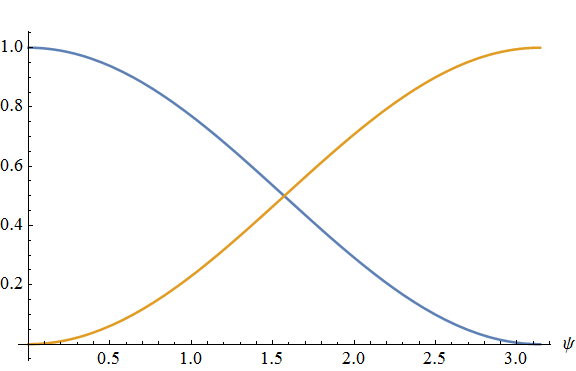
For $c=d=0$ , two simple choices are $a=b=\frac{1}{2}M_{0}$ and $a=-b=\frac{1}{2}M_{0}$ , where $M_{0}$ is the rescaled Planck mass (2). These give the following $\theta$ -independent potentials, which involve only the orbitals $s$ and $p_{z}$ and are shown in Figure 1:

\widehat{\Phi}_{+}(\psi)=M_{0}\cos^{2}\left(\frac{\psi}{2}\right)~~,~~\widehat{\Phi}_{-}(\psi)=M_{0}\sin^{2}\left(\frac{\psi}{2}\right)~~.

(10)

Notice that $\widehat{\Phi}_{+}$ has a maximum at $\psi=0$ (north pole) and a minimum at $\psi=\pi$ (south pole) while $\widehat{\Phi}_{-}$ has a minimum at $\psi=0$ (north pole) and a maximum at $\psi=\pi$ (south pole).

Refer to caption — Figure 1: Plot of $\widehat{\Phi}_{+}/M_{0}$ (blue) and $\widehat{\Phi}_{-}/M_{0}$ (yellow) as functions of $\psi\in[0,\pi]$ . The value $\psi=0$ corresponds to the north pole of $\mathrm{S}^{2}$ , while $\psi=\pi$ corresponds to the south pole.

Another simple choice is $b=d=0$ and $a=c=M_{0}$ , which corresponds to a linear combination of the $s$ and $p_{x}$ orbitals and gives the extended potential:

\widehat{\Phi}_{0}(\psi,\theta)=M_{0}(1+\sin\psi\cos\theta)=M_{0}(1+x_{1})~~.

(11)

Unlike $\widehat{\Phi}_{\pm}$ , this function does not have extrema at the north or south pole. Instead, it has two extrema along the equator of $\mathrm{S}^{2}$ , having a maximum (equal to $2M_{0}$ ) at the point $(\psi,\theta)=(\frac{\pi}{2},0)$ and a minimum (equal to $0$ ) at $(\psi,\theta)=(\frac{\pi}{2},\pi)$ . Notice that $\widehat{\Phi}_{\pm}$ and $\widehat{\Phi}_{0}$ are Morse functions on $\mathrm{S}^{2}$ , so the potentials derived from them on a planar surface (whose end compactification is $\mathrm{S}^{2}$ ) will be compactly Morse in the sense of [1].

A universal approach to globally well-behaved potentials.

The techniques of passing to the end compactification and lifting to the Poincaré half-plane introduced in [1] allow for a uniform treatment of globally well-behaved scalar potentials in generalized $\alpha$ -attractor models for which $(\Sigma,G)$ is geometrically finite. This is summarized in the commutative diagram (12), where $j$ is the smooth embedding of $\Sigma$ into its end compactification $\widehat{\Sigma}$ and $\pi_{\mathbb{H}}$ is the uniformizing map from $\mathbb{H}$ .

(12)

Any smooth real-valued function $\widehat{\Phi}$ defined on $\widehat{\Sigma}$ induces a globally well-behaved scalar potential $\Phi$ on $\Sigma$ through the formula $\Phi=\widehat{\Phi}\circ j$ , while any globally well-behaved scalar potential $\Phi$ on $\Sigma$ lifts to a smooth function ${\widetilde{\Phi}}=\Phi\circ\pi_{\mathbb{H}}$ defined on $\mathbb{H}$ . When the maps $j$ and $\pi_{\mathbb{H}}$ are known, ${\widetilde{\Phi}}$ can be recovered from $\widehat{\Phi}$ as the composition ${\widetilde{\Phi}}=\widehat{\Phi}\circ\chi$ , where $\chi:\mathbb{H}\rightarrow\widehat{\Sigma}$ is the composite map $\chi\stackrel{{\scriptstyle{\rm def.}}}{{=}}j\circ\pi_{\mathbb{H}}$ . Notice that $j$ and $\chi$ are smooth maps, while $\pi_{\mathbb{H}}$ is holomorphic when $\Sigma$ is endowed with the complex structure which corresponds to the conformal class of the metric $G$ . The maps $j,\pi_{\mathbb{H}}$ and $\chi$ differ for distinct geometrically-finite hyperbolic surfaces $(\widehat{\Sigma},G)$ having the same end compactification $\widehat{\Sigma}$ , which means that the same “universal” extended potential $\widehat{\Phi}$ defined on $\widehat{\Sigma}$ can induce markedly different globally well-behaved potentials $\Phi$ and lifted potentials ${\widetilde{\Phi}}$ for different hyperbolic surfaces of the same genus.

When $\Sigma$ is a planar surface, the end compactification $\widehat{\Sigma}$ coincides with the unit sphere and $\widehat{\Phi}$ can be expanded into real spherical harmonics as explained above. This induces uniformly-convergent expansions:

	$\displaystyle\Phi=\sum_{l=0}^{\infty}\sum_{m=-l}^{l}D_{lm}Y_{lm}\circ j$
	$\displaystyle{\widetilde{\Phi}}=\sum_{l=0}^{\infty}\sum_{m=-l}^{l}D_{lm}Y_{lm}\circ\chi$

of $\Phi$ and ${\widetilde{\Phi}}$ . In the next sections, we determine explicitly the maps $j$ , $\pi_{\mathbb{H}}$ and $\chi$ for the planar elementary surfaces $\mathbb{D}$ , $\mathbb{D}^{\ast}$ and ${\mathbb{A}}(R)$ and the maps $\Phi$ and ${\widetilde{\Phi}}$ induced by the choices $\widehat{\Phi}=\widehat{\Phi}_{\pm}$ and $\widehat{\Phi}=\widehat{\Phi}_{0}$ given above. This illustrates how the same function $\widehat{\Phi}$ leads to different dynamics of the generalized $\alpha$ -attractor models associated to distinct planar surfaces. For the three elementary surfaces, we will construct the map $j:\Sigma\rightarrow\widehat{\Sigma}=\mathrm{S}^{2}$ by first diffeomorphically (but not bi-holomorphically !) identifying $\Sigma$ with the complex plane $\mathbb{C}$ of complex coordinate $\zeta$ (or with $\mathbb{C}$ with a point removed) and then identifying the latter with the once- or twice-punctured sphere by using stereographic projection from the north pole of $\mathrm{S}^{2}$ :

\zeta=\cot\left(\frac{\psi}{2}\right)e^{\mathbf{i}\theta}\in\mathbb{C}~~.

(13)

3 Elementary hyperbolic surfaces

A (complete) hyperbolic surface $(\Sigma,G)$ is called elementary if it is conformally-equivalent with a simply-connected or doubly-connected²² 2 A regular domain $\mathcal{D}\subset\mathbb{C}$ is called doubly-connected if its complement in the Riemann sphere has two connected components, which happens iff $\pi_{1}(\mathcal{D})\simeq\mathbb{Z}$ . regular domain contained in the complex plane. This amounts to the condition that the uniformizing surface group $\Gamma$ of $(\Sigma,G)$ is the trivial group or a cyclic subgroup of $\mathrm{PSL}(2,\mathbb{R})$ of parabolic or hyperbolic type.

Any simply connected regular domain is conformally equivalent with the unit disk $\mathbb{D}=\{u\in\mathbb{C}\,|\,|u|<1\}$ (and hence with the upper half plane $\mathbb{H}$ ). Such a domain admits a unique complete hyperbolic metric, known as the Poincaré metric. Any doubly-connected regular domain is conformally equivalent to one of the following, when the latter is endowed with the complex structure inherited from the complex plane:

•

The punctured plane $\mathbb{C}^{\ast}=\mathbb{C}\setminus\{0\}$
•

The punctured unit disk $\mathbb{D}^{\ast}\stackrel{{\scriptstyle{\rm def.}}}{{=}}\mathbb{D}\setminus\{0\}$
•

The annulus ${\mathbb{A}}(R)\stackrel{{\scriptstyle{\rm def.}}}{{=}}\{u\in\mathbb{C}\,\,|\,\,\frac{1}{R}<|u|<R\}$ of modulus $\mu=2\log R>0$ , where $R>1$ .

When endowed with its usual complex structure, the punctured plane does not support a complete hyperbolic metric. On the other hand, the punctured disk $\mathbb{D}^{\ast}$ and annulus ${\mathbb{A}}(R)$ admit uniquely-determined complete hyperbolic metrics. Notice that both $\mathbb{D}^{\ast}$ and ${\mathbb{A}}(R)$ are homeomorphic with (open) cylinders. Due to this fact, the hyperbolic punctured disk $\mathbb{D}^{\ast}$ is also called the parabolic cylinder while the hyperbolic annuli ${\mathbb{A}}(R)$ are also called hyperbolic cylinders [8]. Summarizing, the list of elementary hyperbolic surfaces is as follows:

1.

The hyperbolic disk $\mathbb{D}$ (which is isometric with the Poincaré half-plane $\mathbb{H}$ ).
2.

The hyperbolic punctured disk $\mathbb{D}^{\ast}$ (uniformized to $\mathbb{H}$ by a parabolic cyclic subgroup of $\mathrm{PSL}(2,\mathbb{R})$ ).
3.

The hyperbolic annuli ${\mathbb{A}}(R)$ for $R>1$ (uniformized to $\mathbb{H}$ by a hyperbolic cyclic subgroup of $\mathrm{PSL}(2,\mathbb{R})$ ).

The explicit form of the hyperbolic metric is known in all cases, as is a fundamental polygon [13, 14, 15] for $\mathbb{D}^{\ast}$ and ${\mathbb{A}}(R)$ . This allows one to study the cosmological dynamics of $\alpha$ -attractor models defined by such surfaces either directly on $(\Sigma,G)$ or (as explained in [1]) by lifting to the hyperbolic disk or to the Poincaré half-plane.

For elementary hyperbolic surfaces, the isometry classification of the ends is as follows [1, 8, 16]:

•

The hyperbolic disk $\mathbb{D}$ has a single end, known as a plane end.
•

The hyperbolic punctured disk $\mathbb{D}^{\ast}$ has two ends. One of these is a cusp end, the other being a horn end.
•

The hyperbolic annulus ${\mathbb{A}}(R)$ has two ends, both of which are funnel ends.

All elementary hyperbolic surfaces are planar (i.e. of genus zero). As explained in [1], this implies that their end compactification [10, 11] is the unit sphere $\mathrm{S}^{2}$ . On the other hand, the conformal boundary $\partial_{\infty}^{G}\Sigma$ [1, 17, 18] differs in the three cases:

•

For the hyperbolic disk, we have $\partial_{\infty}\mathbb{D}=\mathrm{S}^{1}$ , where the circle corresponds to the plane end.
•

For the hyperbolic punctured disk, we have $\partial_{\infty}\mathbb{D}^{\ast}=\{0\}\sqcup\mathrm{S}^{1}$ , where the origin corresponds to the cusp end and $\mathrm{S}^{1}$ corresponds to the horn end.
•

For the hyperbolic annulus, we have $\partial_{\infty}{\mathbb{A}}(\mathbb{R})=\mathrm{S}^{1}\sqcup\mathrm{S}^{1}$ , each of the circles corresponding to a funnel end.

Remark.

By a theorem of Hilbert, a complete hyperbolic surface cannot be embedded isometrically into Euclidean 3-space. However, incomplete regions of such a surface can be embedded isometrically (and we shall see examples of such partial embeddings in latter sections). Notice that one can sometimes find isometric embeddings of complete hyperbolic surfaces into non-Euclidean three-space, such as the well-known embedding of the Poincaré disk as a sheet of a hyperboloid defined inside three-dimensional Minkowski space.

4 The hyperbolic disk

The cosmological model defined by the hyperbolic disk $\mathbb{D}$ coincides with the two-field $\alpha$ -attractor model of [7], which was discussed extensively in the literature. The purpose of this section is to show how this fits into the general theory developed in [1].

4.1 Semi-geodesic coordinates

The unit disk $\mathbb{D}=\{u\in\mathbb{C}\,|\,|u|<1\}$ admits a unique complete hyperbolic metric, which is given by:

\mathrm{d}s_{\mathbb{D}}^{2}=\lambda^{2}_{\mathbb{D}}(u,\bar{u})|\mathrm{d}u|^{2}~~,~\mathrm{where}~~\lambda_{\mathbb{D}}(u,\bar{u})=\frac{2}{1-|u|^{2}}~~.

(14)

In polar coordinates given by $\rho=|u|\in(0,1)$ and $\theta=\arg(u)\in(0,2\pi)$ , the metric becomes:

\mathrm{d}s_{\mathbb{D}}^{2}=\frac{4}{(1-\rho^{2})^{2}}\left(\mathrm{d}\rho^{2}+\rho^{2}\mathrm{d}\theta^{2}\right)~~.

Semi-geodesic coordinates $(r,\theta)$ for $\mathbb{D}$ are obtained by the change of variables:

\rho\stackrel{{\scriptstyle{\rm def.}}}{{=}}\tanh\left(\frac{r}{2}\right)\in(0,1)~~\mathrm{i.e.}~~r=2\arctanh(\rho)=\log\frac{1+\rho}{1-\rho}\in(0,+\infty)~~.

This maps the unit disk (diffeomorphically, but not conformally) to the complex plane with polar coordinates $(r,\theta)$ and complex coordinate:

\zeta=re^{\mathbf{i}\theta}=2\arctanh(\rho)e^{\mathbf{i}\theta}

and brings the metric to the form:

\mathrm{d}s_{\mathbb{D}}^{2}=\mathrm{d}r^{2}+\sinh^{2}(r)\mathrm{d}\theta^{2}~~.

(15)

The single end of $\mathbb{D}$ (which is called a plane end) corresponds to $r\rightarrow+\infty$ , while the center of $\mathbb{D}$ corresponds to $r\rightarrow 0$ .

4.2 The end compactification of $\mathbb{D}$

The end compactification $\widehat{\mathbb{D}}$ of the hyperbolic disk coincides with the Alexandroff compactification of the $\zeta$ -plane, which by the stereographic projection (13) is identified with the unit sphere $\mathrm{S}^{2}$ . The north pole $\psi=0$ corresponds to the plane end at $r=|\zeta|\rightarrow\infty$ , while the south pole $\psi=\pi$ corresponds to $r=0$ , i.e. to the center of $\mathbb{D}$ . In spherical stereographic coordinates $(\psi,\theta)$ , the Poincaré metric (15) becomes:

\mathrm{d}s_{\mathbb{D}}^{2}=\frac{1}{4}\frac{\mathrm{d}\psi^{2}}{\sin^{2}(\frac{\psi}{2})}+\sinh^{2}(\cot(\frac{\psi}{2}))\mathrm{d}\theta^{2}~~.

Remark.

The compact Riemann surface into which $\mathbb{D}=\{u\in\mathbb{C}\,|\,|u|<1\}$ embeds holomorphically [17, 18] is the Riemann sphere $\mathbb{C}\mathbb{P}^{1}$ associated to the $u$ -plane. The coordinate $u$ is given by:

u\stackrel{{\scriptstyle{\rm def.}}}{{=}}\frac{u_{1}}{u_{2}}~~\mathrm{for}~~u_{2}\neq 0~~,

where $(u_{1},u_{2})\in\mathbb{C}^{2}\setminus\{0,0\}$ are the homogeneous coordinates of $\mathbb{C}\mathbb{P}^{1}$ .

4.3 Globally well-behaved scalar potentials on $\mathbb{D}$

A potential $\Phi:\mathbb{D}\rightarrow\mathbb{R}$ is globally well-behaved on $\mathbb{D}$ iff there exists a smooth function $\widehat{\Phi}:\mathrm{S}^{2}\rightarrow\mathbb{R}$ such that:

\Phi(r,\theta)=\widehat{\Phi}(2\arccot(r),\theta)~~,

(16)

i.e.:

\Phi(\rho,\theta)=\widehat{\Phi}(2\arccot(2\arctanh\rho),\theta)~~.

The condition that $\widehat{\Phi}$ is smooth on $\mathrm{S}^{2}$ implies, in particular, that $\widehat{\Phi}(\psi,\theta)$ has a finite limit for $\psi\rightarrow 0$ and hence $\Phi(r,\theta)$ has a $\theta$ -independent limit for $r\rightarrow+\infty$ i.e. for $|u|\rightarrow 1$ . Expansion (8) gives the uniformly-convergent series:

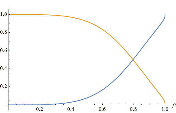
\Phi(\rho,\theta)=\sum_{l=0}^{\infty}\sum_{m=-l}^{l}D_{lm}Y_{lm}(2\arccot(2\arctanh\rho),\theta)~~.

To obtain inflationary behavior with the scalar field rolling from the plane end towards the interior of $\mathbb{D}$ , one can require that $\widehat{\Phi}$ has a local maximum at the north pole of $\mathrm{S}^{2}$ . In the simplest models, one can take $\widehat{\Phi}$ to have only two critical points, namely a global maximum at the north pole and a global minimum at the south pole. In that case, $\Phi$ has a global minimum at $u=0$ (the center of $\mathbb{D}$ ) and increases monotonically to a $\theta$ -independent finite value as $|u|$ grows from zero to $1$ (toward the conformal boundary $\partial_{\infty}\mathbb{D}=\mathrm{S}^{1}$ of $\mathbb{D}$ ).

In polar coordinates $(\rho,\theta)$ , the extended potentials (10) of Section 2 correspond to the following globally well-behaved scalar potentials on $\mathbb{D}$ :

\Phi_{+}=M_{0}\frac{r^{2}}{1+r^{2}}=M_{0}\frac{\left(\log\frac{1+\rho}{1-\rho}\right)^{2}}{1+\left(\log\frac{1+\rho}{1-\rho}\right)^{2}}~~,~~\Phi_{-}=\frac{M_{0}}{1+r^{2}}=\frac{M_{0}}{1+\left(\log\frac{1+\rho}{1-\rho}\right)^{2}}~~,

(17)

where $\rho=|u|$ . These potentials are shown in Figures 2 and 2, which illustrate the characteristic stretching toward the end when the potential is expressed in semi-geodesic coordinates $(r,\theta)$ (with respect to which the two locally-defined real scalar fields of the sigma model have canonical kinetic terms). The supremum of $\Phi_{+}$ corresponds to $\rho\rightarrow 1$ (being equal to $M_{0}$ ), while the infimum is attained at $\rho=0$ (where $\Phi_{+}$ vanishes). On the other hand, $\Phi_{-}$ tends to its vanishing infimum for $\rho\rightarrow 1$ and has a maximum at $\rho=0$ (where it equals $M_{0}$ ). Notice that only $\Phi_{+}$ leads to standard $\alpha$ -attractor behavior.

Using the relation $\sin\psi=2\sin(\psi/2)\cos(\psi/2)=\frac{2r}{1+r^{2}}$ , the choice (11) gives the following potential on $\mathbb{D}$ :

\Phi_{0}=M_{0}\left[1+\frac{2r}{1+r^{2}}\cos\theta\right]=M_{0}\left[1+\frac{2\log\frac{1+\rho}{1-\rho}}{1+\left(\log\frac{1+\rho}{1-\rho}\right)^{2}}\cos\theta\right]~~.

5 The hyperbolic punctured disk

The hyperbolic punctured disk $\mathbb{D}^{\ast}$ (also known as the “parabolic cylinder” [8]) is the simplest example of a hyperbolic surface with a cusp end. It also has a horn end.

5.1 The hyperbolic metric

The punctured unit disk $\mathbb{D}^{\ast}=\{u\in\mathbb{C}\,|\,0<|u|<1\}$ admits a unique complete hyperbolic metric given by [19]:

\mathrm{d}s_{\mathbb{D}^{\ast}}^{2}=\lambda_{\mathbb{D}^{\ast}}^{2}(u,\bar{u})|\mathrm{d}u|^{2}~~,~\mathrm{where}~~\lambda_{\mathbb{D}^{\ast}}(u,\bar{u})=\frac{1}{|u|\log(1/|u|)}~~.

(18)

In particular, $\mathrm{Re}u$ and $\mathrm{Im}u$ are isothermal coordinates. In polar coordinates $(\rho,\theta)$ defined through:

u=\rho e^{\mathbf{i}\theta}~~(\rho=|u|\in(0,1))~~,

the metric takes the form:

\mathrm{d}s_{\mathbb{D}^{\ast}}^{2}=\frac{1}{(\rho\log\rho)^{2}}(\mathrm{d}\rho^{2}+\rho^{2}\mathrm{d}\theta^{2})~~.

The center of $\mathbb{D}^{\ast}$ corresponds to the cusp end, while the bounding circle of $\mathbb{D}^{\ast}$ corresponds to the horn end (see below). The Euclidean circle at $\rho=e^{-2\pi}$ is a horocycle of hyperbolic length $1$ . Notice that $\mathbb{D}^{\ast}$ has infinite hyperbolic area.

5.2 Diffeomorphism to the punctured plane

One can introduce an orthogonal coordinate system $(\mathfrak{r},\theta)\in(0,+\infty)\times(0,2\pi)$ on $\mathbb{D}^{\ast}$ through the coordinate transformation:

\mathfrak{r}\stackrel{{\scriptstyle{\rm def.}}}{{=}}\frac{1}{\log\left(\frac{1}{\rho}\right)}=\frac{1}{|\log\rho|}\in(0,+\infty)~~\mathrm{i.e.}~~\rho=e^{-\frac{1}{\mathfrak{r}}}\in(0,1)~~.

(19)

This gives a diffeomorphism between $\mathbb{D}^{\ast}$ and the punctured complex plane $\mathbb{C}^{\ast}\stackrel{{\scriptstyle{\rm def.}}}{{=}}\mathbb{C}\setminus\{0\}$ with complex coordinate:

\zeta=\mathfrak{r}e^{\mathbf{i}\theta}~~.

In this coordinate system, the metric (18) takes the form:

\mathrm{d}s_{\mathbb{D}^{\ast}}^{2}=\frac{1}{\mathfrak{r}^{2}}\mathrm{d}\mathfrak{r}^{2}+\mathfrak{r}^{2}\mathrm{d}\theta^{2}~~.

(20)

The center of $\mathbb{D}^{\ast}$ corresponds to $\mathfrak{r}\rightarrow 0$ , while the bounding circle of $\mathbb{D}^{\ast}$ corresponds to $\mathfrak{r}\rightarrow+\infty$ .

5.3 Partial isometric embedding into Euclidean 3-space

One can isometrically embed the portion $0<|u|<\frac{1}{e}$ of the hyperbolic punctured disk into Euclidean $\mathbb{R}^{3}$ as the open half-tractricoid³³ 3 The surface obtained by revolving an open half of a tractrix along its asymptote [20]. $\mathcal{E}$ defined in cylindrical coordinates $(\mathfrak{r},\theta,x_{3})$ (where $x_{1}=\mathfrak{r}\cos\theta$ and $x_{2}=\mathfrak{r}\sin\theta$ ) by the parametric equations:

\mathfrak{r}=\frac{1}{\cosh(\mathfrak{t})}\in(0,1)~~,~~x_{3}=\mathfrak{t}-\tanh(\mathfrak{t})~~(\mathfrak{t}\in(0,+\infty))~~.

Indeed, it is easy to see that the Euclidean metric of $\mathbb{R}^{3}$ induces a metric on $\mathcal{E}$ which coincides with (20). This is the classical pseudosphere model of Beltrami (see Figure 3).

5.4 The end compactification of $\mathbb{D}^{\ast}$

The stereographic projection (13) identifies $\mathrm{S}^{2}$ with the one-point compactification of the $\zeta$ -plane. This shows explicitly that $\mathrm{S}^{2}$ is the end compactification of $\mathbb{D}^{\ast}$ , where the north pole $\psi=0$ corresponds to the horn end and the south pole $\psi=\pi$ corresponds to the cusp end. The embedding $j:\mathbb{D}^{\ast}\rightarrow\mathrm{S}^{2}$ is given by:

\psi=2\arctan(|\log\rho|)~~,~~\theta=\theta~~.

5.5 Semi-geodesic coordinates

The further change of variables:

\mathfrak{r}=\frac{1}{2\pi}e^{-r}~~\mathrm{i.e.}~~r=-\log(2\pi\mathfrak{r})=\log\left(\frac{|\log\rho|}{2\pi}\right)\in(-\infty,+\infty)

(21)

brings the metric (20) to the form:

\mathrm{d}s_{\mathbb{D}^{\ast}}^{2}=\mathrm{d}r^{2}+\frac{e^{-2r}}{(2\pi)^{2}}\mathrm{d}\theta^{2}~~,

(22)

where $r\in\mathbb{R}$ . In particular, $(r,\theta)$ are semi-geodesic coordinates. The center $u=0$ of $\mathbb{D}^{\ast}$ corresponds to $r\rightarrow+\infty$ while the bounding circle $|u|=1$ of $\mathbb{D}^{\ast}$ corresponds to $r\rightarrow-\infty$ . The horocycle at $r=0$ (i.e. $\rho=e^{-2\pi}$ ) has length $1$ .

5.6 The hyperbolic cusp

Let:

\kappa\stackrel{{\scriptstyle{\rm def.}}}{{=}}e^{-2\pi}~~.

(23)

As mentioned above, the Euclidean circle $|u|=\kappa$ has hyperbolic length $1$ . The hyperbolic cusp (cf. [1]) corresponds to the portion of $\mathbb{D}^{\ast}$ lying inside this circle (see Figure 3), which is the open punctured disk:

\mathrm{C}\stackrel{{\scriptstyle{\rm def.}}}{{=}}\{u\in\mathbb{C}\,\,|\,\,0<|u|<\kappa\}\subset\mathbb{D}^{\ast}~~,

(24)

endowed with the restriction of the metric (18); notice that the restricted metric is not complete. In coordinates $(\mathfrak{r},\theta)$ , the metric on $\mathrm{C}$ is obtained by restricting (20) to the range $\mathfrak{r}\in(0,\mathfrak{r}_{0})$ , where:

\mathfrak{r}_{0}\stackrel{{\scriptstyle{\rm def.}}}{{=}}\frac{1}{2\pi}~~.

In semi-geodesic coordinates $(r,\theta)$ the cusp metric is given by (22) with the restriction $r\in(0,+\infty)$ . Notice that $\mathrm{C}$ has hyperbolic area equal to $1$ .

5.7 The hyperbolic horn

By definition, the hyperbolic horn is the annulus:

\mathrm{H}=\{u\in\mathbb{C}\,\,|\,\,\kappa<|u|<1\}\subset\mathbb{D}^{\ast}~~,

endowed with the (incomplete) restriction of the metric (18). In coordinates $(\mathfrak{r},\theta)$ , the horn metric is obtained from (20) by restricting the range of $\mathfrak{r}$ to $(\mathfrak{r}_{0},+\infty)$ . In coordinates $(r,\theta)$ , the metric takes the form (22), with the restriction $r\in(-\infty,0)$ . Defining $r^{\prime}\stackrel{{\scriptstyle{\rm def.}}}{{=}}-r$ , this can be brought to the form:

\mathrm{d}s^{2}_{\mathrm{H}}=(\mathrm{d}r^{\prime})^{2}+\frac{e^{2r^{\prime}}}{(2\pi)^{2}}\mathrm{d}\theta^{2}~~,~~\mathrm{with}~~r^{\prime}\in(0,+\infty)~~,

(25)

where the bounding circle $|u|=1$ of $\mathbb{D}^{\ast}$ corresponds to $r^{\prime}\rightarrow+\infty$ .

5.8 Canonical uniformization to $\mathbb{H}$

The punctured disk is uniformized to the Poincaré half-plane (1) with complex coordinate $\tau$ by the parabolic cyclic group $\Gamma_{P}\stackrel{{\scriptstyle{\rm def.}}}{{=}}\langle P\rangle\subset\mathrm{PSL}(2,\mathbb{R})$ generated by the translation:

\tau\rightarrow\tau+1~~,

(26)

which corresponds to the parabolic element:

P\stackrel{{\scriptstyle{\rm def.}}}{{=}}\left[\begin{array}[]{cc}1&1\\ 0&1\end{array}\right]\in\mathrm{PSL}(2,\mathbb{R})~~.

(27)

This fixes the point $\tau=\infty\in\partial_{\infty}\mathbb{H}$ . The uniformization map is:

u=\pi_{\mathbb{H}}(\tau)=e^{2\pi\mathbf{i}\tau}~~.

(28)

The hyperbolic cusp $\mathrm{C}$ is the projection through $\pi_{\mathbb{H}}$ of the cusp domain:

\mathcal{C}_{\mathbb{H}}=\{\tau\in\mathbb{H}|\mathrm{Im}\tau>1\}~~,

which is bounded by the horocycle:

c_{\mathbb{H}}=\{\tau\in\mathbb{H}|\mathrm{Im}\tau=1\}~~.

This horocycle is tangent to the conformal boundary of $\mathbb{H}$ at the point $\tau=\infty$ , which projects through $\pi_{\mathbb{H}}$ to the cusp ideal point of the end compactification of $\mathbb{D}^{\ast}$ .

A fundamental polygon for the action of $\Gamma_{P}$ on $\mathbb{H}$ is given by the semi-infinite vertical strip:

\mathfrak{D}_{\mathbb{H}}=\left\{\tau\in\mathbb{H}\,|\,0<\mathrm{Re}\tau<1\right\}~~,

(29)

and has vertices at the points (see Figure 4):

A:\{\tau=\infty\}~,~B:\{\tau=0\}~,~C:\{\tau=1\}~~.

(30)

The Poincaré side pairing maps $(AB)$ into $(AC)$ through the transformation (26), which generates $\Gamma_{P}$ . The relative cusp neighborhood [1] with respect to $\mathfrak{D}_{\mathbb{H}}$ is the intersection $\mathfrak{C}_{\mathbb{H}}\stackrel{{\scriptstyle{\rm def.}}}{{=}}\mathcal{C}_{\mathbb{H}}\cap\mathfrak{D}_{\mathbb{H}}$ . A lifted scalar potential ${\widetilde{\Phi}}=\Phi\circ\pi_{\mathbb{H}}$ is given by:

{\widetilde{\Phi}}(\tau)=\Phi(e^{2\pi i\tau})~~,

being invariant under the translation (26). In particular, the restrictions of ${\widetilde{\Phi}}$ to the sides $(AB)$ and $(AC)$ agree through the Poincaré pairing.

5.9 Canonical uniformization to $\mathbb{D}$

For completeness and comparison with [1], we also give the canonical uniformization of $\mathbb{D}^{\ast}$ to the hyperbolic disk. The Cayley transformation:

u=\frac{\mathbf{i}-\tau}{\mathbf{i}\tau-1}

(31)

is an isometry from $\mathbb{H}$ to $\mathbb{D}$ . When uniformizing $\mathbb{D}^{\ast}$ to $\mathbb{D}$ , the fundamental polygon $\mathfrak{D}_{\mathbb{H}}$ becomes a hyperbolic triangle $\mathfrak{D}_{\mathbb{D}}$ with vertices at the following points, which correspond respectively to the points $A$ , $B$ and $C$ of (30) through the Cayley transformation:

A^{\prime}:\{u=\mathbf{i}\}~,~B^{\prime}:\{u=-\mathbf{i}\}~,~~C^{\prime}:\{u=1\}

and a free side connecting the points $B^{\prime}$ and $C^{\prime}$ (see Figure 4). The sides of this triangle are a segment connecting $A^{\prime}$ to $B^{\prime}$ (which passes through the origin of $\mathbb{D}$ ), the portion of $\partial_{\infty}\mathbb{D}$ connecting $B^{\prime}$ to $C^{\prime}$ and a Euclidean circular arc orthogonal to $\partial_{\infty}\mathbb{D}$ which connects $A^{\prime}$ to $C^{\prime}$ . The hyperbolic cusp neighborhood $\mathcal{C}_{\mathbb{D}}$ of the vertex $A^{\prime}$ is bounded by the horocycle:

c_{\mathbb{D}}=\left\{\frac{t}{2-\mathbf{i}t}\in\mathfrak{D}_{\mathbb{D}}\,|\,t\in\mathbb{R}\right\}~~,

which is tangent to $\partial_{\infty}\mathbb{D}$ at the point $A^{\prime}$ . The intersection of $\mathcal{C}_{\mathbb{D}}$ with $\mathfrak{D}_{\mathbb{D}}$ is the relative cusp neighborhood $\mathfrak{C}_{\mathbb{D}}$ with respect to $\mathfrak{D}_{\mathbb{D}}$ (see [1]), which is the image of $\mathfrak{C}_{\mathbb{H}}$ through the Cayley transformation.

5.10 Globally well-behaved scalar potentials on $\mathbb{D}^{\ast}$

A scalar potential $\Phi:\Sigma\rightarrow\mathbb{R}$ is globally well-behaved on $\mathbb{D}^{\ast}$ iff there exists a smooth map $\widehat{\Phi}:\mathrm{S}^{2}\rightarrow\mathbb{R}$ such that:

\Phi(\mathfrak{r},\theta)=\widehat{\Phi}(2\arccot(\mathfrak{r}),\theta)~~,

i.e.:

\Phi(\rho,\theta)=\widehat{\Phi}(2\arctan(|\log\rho|),\theta)~~,

where $\rho=|u|$ . Expansion (8) gives the uniformly-convergent series:

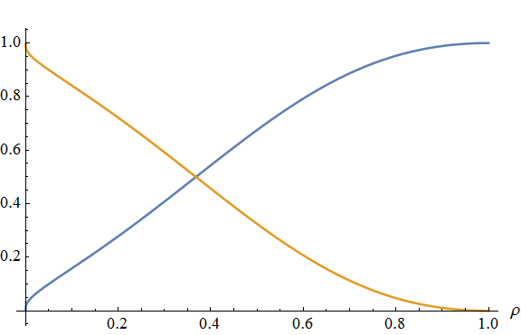
\Phi(\rho,\theta)=\sum_{l=0}^{\infty}\sum_{m=-l}^{l}D_{lm}Y_{lm}(2\arctan(|\log\rho|),\theta)~~.

For the choices (10) and (11), we find:

	$\displaystyle\Phi_{+}=M_{0}\frac{\mathfrak{r}^{2}}{1+\mathfrak{r}^{2}}=M_{0}\frac{1}{1+(\log\rho)^{2}}$
	$\displaystyle\Phi_{-}=M_{0}\frac{1}{1+\mathfrak{r}^{2}}=M_{0}\frac{(\log\rho)^{2}}{1+(\log\rho)^{2}}$		(32)
	$\displaystyle\Phi_{0}=M_{0}\left[1+\frac{2\mathfrak{r}\cos\theta}{1+\mathfrak{r}^{2}}\right]=M_{0}\left[1+\frac{2\|\log\rho\|}{1+(\log\rho)^{2}}\cos\theta\right]~~.$

These potentials are shown in Figure 5. Notice that $\Phi_{+}$ leads to $\alpha$ -attractor behavior if inflation takes place near the horn end, while $\Phi_{-}$ leads to $\alpha$ -attractor behavior if inflation takes place near the cusp end [1]. The extended potentials $\widehat{\Phi}_{\pm}$ have maxima and minima at the two ideal points of the end compactification of $\mathbb{D}^{\ast}$ (which correspond to the north and south poles of $\mathrm{S}^{2}$ ). On the other hand, $\widehat{\Phi}_{0}$ does not have extrema at the ideal points; its extrema coincide with those of $\Phi_{0}$ , being located inside $\mathbb{D}^{\ast}$ . The minimum (equal to zero) is at the point $u=-\frac{1}{e}\approx-0.36$ while the maximum (equal to $2M_{0}$ ) is at $u=+\frac{1}{e}\approx+0.36$ .

Remark.

Using (21), we find the following expressions in semi-geodesic coordinates:

\Phi_{+}(r)=\frac{M_{0}}{1+(2\pi)^{2}e^{2r}}~~,~~\Phi_{-}(r)=\frac{M_{0}}{1+\frac{e^{-2r}}{(2\pi)^{2}}}~~,~~\Phi_{0}(r,\theta)=M_{0}\left[1+\frac{4\pi e^{-r}\cos\theta}{(2\pi)^{2}+e^{-2r}}\right]~~.

(33)

Lift of the potentials $\Phi_{\pm}$ and $\Phi_{0}$ to $\mathbb{H}$ .

Consider the well-behaved scalar potentials $\Phi_{\pm}$ and $\Phi_{0}$ on $\mathbb{D}^{\ast}$ given in (32). Let $x=\mathrm{Re}\tau$ and $y\stackrel{{\scriptstyle{\rm def.}}}{{=}}\mathrm{Im}\tau$ . Then the covering map (28) reads:

u=\pi_{\mathbb{H}}(\tau)=e^{2\pi\mathbf{i}\tau}=e^{-2\pi y}[\cos(2\pi x)+\mathbf{i}\sin(2\pi x)]~~,

which gives:

\rho=|u|=e^{-2\pi y}~~,~~\theta=\arg(u)=2\pi x~(\mathrm{mod}\,2\pi)~~.

(34)

Hence the potentials $\Phi_{\pm}$ and $\Phi_{0}$ have the following lifts to $\mathbb{H}$ (see Figure 6):

{\widetilde{\Phi}}_{+}=M_{0}\frac{1}{1+(2\pi)^{2}y^{2}}~~,~~{\widetilde{\Phi}}_{-}=M_{0}\frac{y^{2}}{(2\pi)^{-2}+y^{2}}~~,~~{\widetilde{\Phi}}_{0}=M_{0}\left[1+\frac{4\pi y\cos(2\pi x)}{1+4\pi^{2}y^{2}}\right]~~.

(35)

The function ${\widetilde{\Phi}}_{0}(\tau)$ (which is periodic under $\tau\rightarrow\tau+1$ ) attains its minimum $\min{\widetilde{\Phi}}_{0}=0$ at the points $\tau=n+\frac{1}{2}+\frac{\mathbf{i}}{2\pi}\approx n+0.5+0.16\mathbf{i}$ (with $n\in\mathbb{Z}$ ), while the maximum $\max{\widetilde{\Phi}}_{0}=2M_{0}$ is attained for $\tau=n+\frac{\mathbf{i}}{2\pi}\approx n+0.16\mathbf{i}$ with $n\in\mathbb{Z}$ .

5.11 Cosmological trajectories on the hyperbolic punctured disk

In this subsection, we present examples of numerically-computed trajectories on $\mathbb{D}^{\ast}$ for the vanishing scalar potential and for the globally well-behaved scalar potentials $\Phi_{\pm}$ and $\Phi_{0}$ . These were obtained as explained in Subsection 1.2, by numerically computing solutions of the system (5) on the Poincaré half-plane for the corresponding lifted potentials and then projecting these trajectories to the hyperbolic punctured disk using the explicitly-known uniformization map (28) (which is equivalent with (34)).

Trajectories for vanishing scalar potential.

To understand the effect of the hyperbolic metric on the dynamics, we start with the case of a vanishing scalar potential $\Phi=0$ . Then ${\widetilde{\Phi}}=0$ and one immediately checks that straight lines given by constant functions $x(t)=x_{0},y(t)=y_{0}$ are solutions of (4) for any initial point $(x_{0},y_{0})\in\mathbb{H}$ , with initial velocity zero. This means that a scalar field starting “at rest” remains at rest for all times. On the other hand, numerical computation shows that any solution of (4) tends to the real axis for $t\rightarrow+\infty$ , irrespective of its initial conditions. As a consequence, any solution defined on $\mathbb{D}^{\ast}$ (which is obtained by projecting a solution defined on $\mathbb{H}$ through the map (28)) will tend toward the horn end as $t\rightarrow+\infty$ . This shows that the hyperbolic metric acts as an effective force which repulses $\varphi$ away from the cusp end. Notice that a global trajectory defined on $\mathbb{D}^{\ast}$ can have cusp and self-intersection points and hence that it need not correspond to an embedded curve in $\mathbb{D}^{\ast}$ .

Figure 7 shows five trajectories on $\mathbb{H}$ and their projections to $\mathbb{D}^{\ast}$ for $\Phi=0$ and $\alpha=\frac{M_{0}}{3}$ , with the following initial conditions:

trajectory	$\tau_{0}$	$\widetilde{v}_{0}$
orange	$0.3+0.159\,\mathbf{i}$	$0$
yellow	$0.01+0.009\,\mathbf{i}$	$0$
red	$0.1+0.2\,\mathbf{i}$	$2+3\,\mathbf{i}$
blue	$\mathbf{i}$	$1+\,\mathbf{i}$
magenta	$0.1\,\mathbf{i}$	$1.3+7\,\mathbf{i}$

Table 1: Initial conditions for five trajectories on the Poincaré half-plane.

Trajectories for $\Phi_{-}$ .

Five lifted trajectories (and their projections to $\mathbb{D}^{\ast}$ ) for $\alpha=\frac{M_{0}}{3}$ and $\Phi=\Phi_{-}$ with the initial conditions given in Table 1 are shown in Figure 8. Since $\widehat{\Phi}_{-}$ has a maximum at the cusp end (center of the disk) and a minimum at the horn end, it reinforces the effect of the hyperbolic metric, together with which it produces an effective repulsion away from the cusp end. In particular, the two trajectories which start with vanishing initial velocity are no longer stationary, but evolve for $t\rightarrow+\infty$ to the funnel end (see the orange and yellow trajectories in the figures). Any other trajectory (irrespective of its initial velocity) also evolves for $t\rightarrow+\infty$ to the funnel end.

Trajectories for $\Phi_{+}$ .

Five lifted trajectories for $\alpha=\frac{M_{0}}{3}$ and $\Phi=\Phi_{+}$ (and their projections to $\mathbb{D}^{\ast}$ ) with the initial conditions given in Table 1 are shown in Figure 9. Since $\widehat{\Phi}_{+}$ has a minimum at the cusp end (which corresponds to the center of the disk), it produces an attractive force towards the cusp end, which acts as a counterbalance to the repulsive effect of the hyperbolic metric.

Trajectories for $\Phi_{0}$ .

Five lifted trajectories (and their projections to $\mathbb{D}^{\ast}$ ) for $\alpha=\frac{M_{0}}{3}$ and $\Phi=\Phi_{0}$ with the initial conditions given in Table 1 are shown in Figure 10.

Figure 11 shows in more detail the behavior of the magenta trajectory of Figure 10 near the local minimum of ${\widetilde{\Phi}}_{0}$ located at $\tau=\frac{3}{2}+\frac{\mathbf{i}}{2\pi}$ (which projects to $u=-\frac{1}{e}$ ) and of its projection to $\mathbb{D}^{\ast}$ . For this solution, $\varphi$ evolves in a spiral around the minimum of $\Phi_{0}$ , until it settles at the minimum.

5.12 Inflationary regions and number of e-folds

Recall from [21] the expressions for the Hubble parameter and the critical Hubble parameter:

H(t)=\frac{1}{3M_{0}}\sqrt{3\alpha\frac{\dot{x}(t)^{2}+\dot{y}(t)^{2}}{y(t)^{2}}+2{\widetilde{\Phi}}(x(t),y(t))}~~,

(36)

H_{c}(t)=\frac{1}{M_{0}}\sqrt{\frac{{\widetilde{\Phi}}(t)}{3}}~.

(37)

For the inflationary regions the following inequality should be satisfied:

H(t)<H_{c}(t)~,

(38)

while the number of e-folds ${N}$ is given by integrating $H(t)$ over the first inflationary time interval $t_{I}$ :

{N}=\int_{0}^{t_{I}}H(t)\mathrm{d}t~.

(39)

Analyzing the five trajectories with the initial conditions given in Table 1, we find that only the orange and yellow trajectories start in inflationary regime for each of the three potentials $\Phi_{+},\Phi_{-},\Phi_{0}$ , while the other three trajectories do not start in inflationary regime for any of these potentials. We also notice that the yellow trajectory in $\Phi_{0}$ is in inflationary regime for all times. Calculating the number of e-folds, we find for the orange trajectory the values $0.44$ for the potential $\Phi_{0}$ and $0.75$ for $\Phi_{\pm}$ , while the yellow trajectory has $55$ e-folds for the potential $\Phi_{+}$ (so it satisfies the observational requirement of $50-60$ e-folds) and $0.3$ for $\Phi_{-}$ . Varying the initial conditions of the yellow trajectory in the potential $\Phi_{+}$ (namely varying $\mathrm{Im}\tau_{0}$ in the range $[0.0094,0.0096]$ ) produces many other trajectories with $N$ lying in the observationally expected range of $[50,60]$ e-folds.

6 Hyperbolic annuli

Hyperbolic annuli (also known as “hyperbolic cylinders” [8]) have a single modulus and two funnel ends.

6.1 The hyperbolic metric

Let $R>1$ be a real number. The annulus ${\mathbb{A}}(R)=\{u\in\mathbb{C}\,|\,\frac{1}{R}<|u|<R\}$ of modulus $\mu=2\log R>0$ admits a unique complete hyperbolic metric, which is given by [19]:

\mathrm{d}s_{R}^{2}=\lambda_{R}(u,\bar{u})^{2}|\mathrm{d}u|^{2}~~,~\mathrm{where}~~\lambda_{R}(u,\bar{u})=\frac{\pi}{2\log R}\frac{1}{|u|\cos\left(\frac{\pi\log|u|}{2\log R}\right)}~~.

(40)

In particular, $\mathrm{Re}u$ and $\mathrm{Im}u$ are isothermal coordinates. Notice that the transformation $u\rightarrow\frac{1}{\bar{u}}$ is an isometry. In polar coordinates $(\rho,\theta)$ defined through:

u=\rho e^{\mathbf{i}\theta}~,~\mathrm{with}~~\rho=|u|\in(\frac{1}{R},R)~~,

the metric takes the form:

\mathrm{d}s_{R}^{2}=\left(\frac{\pi}{2\log R}\right)^{2}\frac{\mathrm{d}\rho^{2}+\rho^{2}\mathrm{d}\theta^{2}}{\left[\rho\cos\left(\frac{\pi\log\rho}{2\log R}\right)\right]^{2}}~~.

(41)

For any $\rho\in(1/R,R)$ , the Euclidean circle $c_{\rho}\stackrel{{\scriptstyle{\rm def.}}}{{=}}\{u\in\mathbb{C}||u|=\rho\}$ has hyperbolic circumference given by:

\ell_{R}(c_{\rho})=\frac{\pi^{2}}{(\log R)\cos\left(\frac{\pi\log\rho}{2\log R}\right)}~~.

We have:

\ell_{R}(c_{\rho})=\ell_{R}(c_{1/\rho})~~.

Notice that $\ell_{R}(c_{\rho})$ increases from $\frac{\pi^{2}}{\log R}$ to infinity as $\rho$ increases from $1$ to $R$ and as $\rho$ decreases from $1$ to $1/R$ . In particular, the minimum hyperbolic length is attained for the circle $c_{1}$ of Euclidean radius $\rho=1$ , which is the only closed hyperbolic geodesic of ${\mathbb{A}}(R)$ and has hyperbolic length:

\ell\stackrel{{\scriptstyle{\rm def.}}}{{=}}\ell_{R}(c_{1})=\frac{\pi^{2}}{\log R}=\frac{2\pi^{2}}{\mu}~~,

(42)

known as the hyperbolic circumference of ${\mathbb{A}}(R)$ . The lines:

\{te^{i\theta}|t\in(1/R,R)\}

are geodesics of infinite length. Notice that the hyperbolic area of ${\mathbb{A}}(R)$ is infinite. Relation (42) gives:

R=R_{\ell}=e^{\frac{~\pi^{2}}{\ell}}~~.

(43)

6.2 Diffeomorphism to the punctured disk and to the punctured plane

The annulus ${\mathbb{A}}(R)$ is diffeomorphic (but not biholomorphic !) with the punctured unit disk with complex coordinate $u^{\prime}$ through the map:

u^{\prime}=f(u)=\frac{|u|-\frac{1}{R}}{(R-\frac{1}{R})|u|}u\in\mathbb{D}^{\ast}~~(u\in{\mathbb{A}}(R))~~,

(44)

whose inverse is given by:

u=f^{-1}(u^{\prime})=\frac{(R-\frac{1}{R})|u^{\prime}|+\frac{1}{R}}{|u^{\prime}|}u^{\prime}\in{\mathbb{A}}(R)~~(u^{\prime}\in\mathbb{D}^{\ast})~~.

Notice that $f$ maps the Euclidean circle $|u|=\frac{1}{R}$ to $u^{\prime}=0$ and the Euclidean circle $|u|=R$ to the Euclidean circle $|u^{\prime}|=1$ . Composing $f$ with the map (19) gives a diffeomorphism from ${\mathbb{A}}(R)$ to the punctured complex plane with coordinate:

\zeta=\mathfrak{r}e^{\mathbf{i}\theta}~~,

where:

\mathfrak{r}=-\frac{1}{\log|u^{\prime}|}=\frac{1}{\log\frac{R-\frac{1}{R}}{|u|-\frac{1}{R}}}=\frac{1}{\log\frac{R-\frac{1}{R}}{\rho-\frac{1}{R}}}~~.

(45)

The funnel end at $|u|=\frac{1}{R}$ corresponds to $\zeta=0$ while the funnel end at $|u|=R$ corresponds to $\zeta=\infty$ .

6.3 The end compactification of ${\mathbb{A}}(R)$

The end compactification of ${\mathbb{A}}(R)$ is the unit sphere $\mathrm{S}^{2}$ with polar coordinates $(\psi,\theta)\in(0,\pi)\times(0,2\pi)$ , which maps to the $\zeta$ -plane through the stereographic projection (13). The funnel end at $|u|=\frac{1}{R}$ corresponds to the south pole, while the funnel end at $|u|=R$ corresponds to the north pole. The explicit embedding of ${\mathbb{A}}(R)$ into $\mathrm{S}^{2}$ is given by:

\psi=2\arctan\left(\log\frac{R-\frac{1}{R}}{\rho-\frac{1}{R}}\right)~~,~~\theta=\theta~~.

6.4 The hyperbolic funnel

Let $\ell>0$ be a positive real number and $R_{\ell}$ be defined as in (43). By definition, a hyperbolic funnel (cf. [1]) of circumference $\ell>0$ is the annulus:

\mathrm{F}_{\ell}=\{u\in\mathbb{C}\,\,|\,\,\frac{1}{R_{\ell}}<|u|<1\}\subset{\mathbb{A}}(R_{\ell})~~,

(46)

endowed with the restriction of the metric (40). Since $u\rightarrow\frac{1}{\bar{u}}$ is an isometry of ${\mathbb{A}}(R)$ , the funnel is isometric with the annulus $1<|u|<R_{\ell}$ (endowed with the restriction of (40)). Hence ${\mathbb{A}}(R)$ decomposes as the disjoint union of two funnels and the closed geodesic $c_{1}$ . Notice that a funnel has infinite hyperbolic area. The funnel is diffeomorphic (but not conformally equivalent !) with the punctured unit disk through the map:

u^{\prime}=\frac{|u|-\frac{1}{R_{\ell}}}{(1-\frac{1}{R_{\ell}})|u|}u\in\mathbb{D}^{\ast}~~(u\in\mathrm{F}_{\ell})~~,

(47)

which takes the funnel end $u\rightarrow\frac{1}{R_{\ell}}$ to the center $u^{\prime}\rightarrow 0$ of the unit disk and the circle $c_{1}$ into the bounding circle of the unit disk.

6.5 Semi-geodesic coordinates on $\mathrm{F}_{\ell}$

Consider orthogonal coordinates $(q,\theta)$ on $\mathrm{F}_{\ell}$ given by:

q=\frac{\pi}{\mu}\frac{1}{\cos(\frac{\pi}{\mu}\log\rho)}\in(\frac{\pi}{\mu},+\infty)~~,

where $\rho=|u|$ and $\theta\in(0,2\pi)$ is the polar angle in the $u$ -plane. The limit $\rho\rightarrow 1/R$ corresponds to $q\rightarrow\infty$ , while $\rho\rightarrow 1$ corresponds to $q\rightarrow\frac{\pi}{\mu}=\frac{\ell}{2\pi}$ . In these coordinates, the metric on $\mathrm{F}_{\ell}$ becomes:

\mathrm{d}s_{\mathrm{F}_{\ell}}^{2}=\frac{1}{q^{2}-\left(\frac{\pi}{\mu}\right)^{2}}\mathrm{d}q^{2}+q^{2}\mathrm{d}\theta^{2}=\frac{1}{q^{2}-\left(\frac{\ell}{2\pi}\right)^{2}}\mathrm{d}q^{2}+q^{2}\mathrm{d}\theta^{2}~~.

(48)

The coordinates $\theta$ and:

r\stackrel{{\scriptstyle{\rm def.}}}{{=}}\arccosh\left(\frac{2\pi}{\ell}q\right)=\arccosh\left[\frac{1}{\cos(\frac{\pi}{\mu}\log\rho)}\right]\in(0,+\infty)

(49)

are semi-geodesic on $\mathrm{F}_{\ell}$ . In these coordinates, the metric takes the form:

\mathrm{d}s_{\mathrm{F}_{\ell}}^{2}=\mathrm{d}r^{2}+\frac{\ell^{2}}{(2\pi)^{2}}\cosh^{2}(r)\mathrm{d}\theta^{2}~~.

(50)

The limit $\rho\rightarrow 1/R$ corresponds to $r\rightarrow+\infty$ while $\rho\rightarrow 1$ corresponds to $r\rightarrow 0$ . The parameter $\ell>0$ is the hyperbolic length of the geodesic at $r=0$ .

6.6 Partial isometric embedding of the funnel into Euclidean 3-space

One can isometrically embed the annulus $\mathrm{F}_{\ell}^{0}\subset\mathrm{F}_{\ell}$ corresponding to the range:

\frac{\ell}{2\pi}=\frac{\pi}{\mu}<q\leq\sqrt{1+\left(\frac{\pi}{\mu}\right)^{2}}=\sqrt{1+\left(\frac{\ell}{2\pi}\right)^{2}}

into Euclidean $\mathbb{R}^{3}$ as the surface of revolution defined by the parametric equations (see (20, Chap. 3C) or (22, Chap. 15)):

x_{1}=q(r)\cos\theta~~,~~x_{2}=q(r)\sin\theta~,~~x_{3}=\xi(r)~~,~\mathrm{with}~~r\in\left(0,\arcsinh\left(\frac{2\pi}{\ell}\right)\right)~~,

where:

	$\displaystyle q(r)$	$\displaystyle=$	$\displaystyle\frac{\ell}{2\pi}\cosh(r)\in\left(\frac{\ell}{2\pi},\sqrt{1+\left(\frac{\ell}{2\pi}\right)^{2}}\right)~~(\mathrm{see}~~\eqref{rq})$
	$\displaystyle\xi(r)$	$\displaystyle\stackrel{{\scriptstyle{\rm def.}}}{{=}}$	$\displaystyle\int_{0}^{r}\mathrm{d}r^{\prime}\sqrt{1-\left(\frac{\ell}{2\pi}\right)^{2}\sinh^{2}(r^{\prime})}=-\mathbf{i}\,\mathrm{E}\left(\mathbf{i}r\,,-\left(\frac{\ell}{2\pi}\right)^{2}\right)~~,$

and $\mathrm{E}(\tau,m)$ denotes the elliptic integral of the second kind. This is one of the three⁴⁴ 4 The other two are the pseudosphere/tractricoid (which corresponds to a portion of the hyperbolic cusp) and the surface of “conical type”. types of (incomplete) classical surfaces of revolution in $\mathbb{R}^{3}$ of constant Gaussian curvature equal to $-1$ , namely a surface of “hyperboloid type” (see Figure 14).

6.7 Canonical uniformization to $\mathbb{H}$

The hyperbolic annulus ${\mathbb{A}}(R_{\ell})$ is uniformized to the upper half plane by the hyperbolic cyclic subgroup generated by the transformation:

\tau\rightarrow e^{\ell}\tau~~,

(51)

which corresponds to the hyperbolic element:

H_{\ell}\stackrel{{\scriptstyle{\rm def.}}}{{=}}\left[\begin{array}[]{cc}e^{\ell/2}&0\\ 0&e^{-\ell/2}\end{array}\right]\in\mathrm{PSL}(2,\mathbb{R})~~

(52)

and fixes the points $\tau=0$ and $\tau=\infty$ lying on $\partial_{\infty}\mathbb{H}$ . The uniformization map is:

u=\pi_{\mathbb{H}}(\tau)=R_{\ell}e^{\frac{2\pi i}{\ell}\log\tau}=e^{\frac{\pi^{2}}{\ell}+\frac{2\pi i}{\ell}\log\tau}~~,

(53)

which gives:

\rho=e^{\frac{\pi^{2}}{\ell}-\frac{2\pi}{\ell}\arg(\tau)}~~,~~\theta=\frac{2\pi}{\ell}\log|\tau|~~(\mathrm{mod}~2\pi)~~.

(54)

A fundamental polygon is given by (see Figure 15):

\mathfrak{D}_{\mathbb{H}}=\left\{\tau\in\mathbb{H}\,\,|\,\,e^{l}<|\tau|<e^{2l}\right\}~~,~~l>0~~.

(55)

This is a hyperbolic quadrilateral with two free sides and vertices located at the points:

A:\{\tau=-e^{2\ell}\}~,~B:\{\tau=-e^{\ell}\}~,~C:\{\tau=e^{\ell}\}~~,~~D:\{\tau=e^{2\ell}\}~~.

(56)

The funnel $\mathrm{F}_{\ell}$ is the projection of the relative funnel neighborhood [1]:

\mathfrak{F}_{\mathbb{H}}^{\ell}=\{\tau\in\mathfrak{D}_{\mathbb{H}}|\mathrm{Re}\tau<0\}=\{\tau\in\mathfrak{D}_{\mathbb{H}}|\arg(\tau)\in\left(\frac{\pi}{2},\pi\right)\}~~.

6.8 Canonical uniformization to $\mathbb{D}$

When passing to the disk model, the fundamental domain $\mathfrak{D}_{\mathbb{H}}$ is mapped by the Cayley transformation (31) to a hyperbolic quadrilateral $\mathfrak{D}_{\mathbb{D}}$ with vertices located at the following points, which are obtained from the points $A,B,C,D$ defined in (56) by applying (31):

A^{\prime}:\{u=-\frac{\mathbf{i}+e^{2l}}{\mathbf{i}e^{2l}+1}\}~~,~~B^{\prime}:\{u=-\frac{\mathbf{i}+e^{l}}{\mathbf{i}e^{l}+1}\}~~,~~C^{\prime}:\{u=\frac{\mathbf{i}-e^{l}}{\mathbf{i}e^{l}-1}\}~~,~~D^{\prime}:u=\{\frac{\mathbf{i}-e^{2l}}{\mathbf{i}e^{2l}-1}\}~~.

The free sides $(A^{\prime}B^{\prime})$ and $(C^{\prime}D^{\prime})$ are portions of $\partial_{\infty}\mathbb{D}$ (see Figure 15), while the sides $(B^{\prime}C^{\prime})$ and $(A^{\prime}D^{\prime})$ are arc segments of Euclidean circles which are orthogonal to $\partial_{\infty}\mathbb{D}$ .

6.9 Globally well-behaved scalar potentials on ${\mathbb{A}}(R)$

A scalar potential $\Phi$ on ${\mathbb{A}}(R)$ is globally well-behaved iff there exists a smooth function $\widehat{\Phi}:\mathrm{S}^{2}\rightarrow\mathbb{R}$ such that:

\Phi(\mathfrak{r},\theta)=\widehat{\Phi}(2\arccot(\mathfrak{r}),\theta)~~,

i.e.:

\Phi(\rho,\theta)=\widehat{\Phi}\left(2\arctan\left(\log\frac{R-\frac{1}{R}}{\rho-\frac{1}{R}}\right),\theta\right)~~.

Expansion (8) gives the uniformly-convergent series:

\Phi(\rho,\theta)=\sum_{l=0}^{\infty}\sum_{m=-l}^{l}D_{lm}Y_{lm}\left(2\arctan\left(\log\frac{R-\frac{1}{R}}{\rho-\frac{1}{R}}\right),\theta\right)~~.

For the choices (10), we find:

\Phi_{+}=M_{0}\frac{\mathfrak{r}^{2}}{1+\mathfrak{r}^{2}}=M_{0}\frac{1}{1+\left[\log\frac{R-\frac{1}{R}}{\rho-\frac{1}{R}}\right]^{2}}~~,~~\Phi_{-}=M_{0}\frac{1}{1+\mathfrak{r}^{2}}=M_{0}\frac{\left[\log\frac{R-\frac{1}{R}}{\rho-\frac{1}{R}}\right]^{2}}{1+\left[\log\frac{R-\frac{1}{R}}{\rho-\frac{1}{R}}\right]^{2}}~~,

(57)

where $\rho=|u|\in(\frac{1}{R},R)$ and we used (45). The potentials $\Phi_{\pm}$ are plotted in Figure 16 for the case $\ell=\pi^{2}$ ( $R=e$ ). For the choice (11), we find:

\Phi_{0}=M_{0}\left[1+\frac{2\mathfrak{r}}{1+\mathfrak{r}^{2}}\cos\theta\right]=M_{0}\left[1+\frac{2\log\frac{R-\frac{1}{R}}{\rho-\frac{1}{R}}}{1+\left(\log\frac{R-\frac{1}{R}}{\rho-\frac{1}{R}}\right)^{2}}\cos\theta\right]~~.

(58)

Recall that $\widehat{\Phi}_{0}$ has two extrema on $\mathrm{S}^{2}$ , which are located at $(\psi,\theta)=(\frac{\pi}{2},0)$ (maximum) and $(\psi,\theta)=(\frac{\pi}{2},\pi)$ (minimum). At each of these points, relation (13) gives $\mathfrak{r}=\cot(\frac{\pi}{4})=1$ , so (45) gives $\rho=\rho_{0}$ , where:

\rho_{0}\stackrel{{\scriptstyle{\rm def.}}}{{=}}\frac{1}{R}+\frac{1}{e}(R-\frac{1}{R})~~.

(59)

It follows that the two critical points of $\Phi_{0}$ on ${\mathbb{A}}(R)$ are located on the real axis at:

•

$u_{M}=+\rho_{0}$ , where $\Phi_{0}$ attains its maximum (which equals $2M$ )
•

$u_{m}=-\rho_{0}$ , where $\Phi_{0}$ attains its minimum (which equals zero).

The level curves of $\Phi_{0}$ are shown in Figure 16 for the case $\ell=\pi^{2}$ ( $R=e$ ), which gives $\rho_{0}=\frac{e^{2}+e-1}{e^{2}}=1+\frac{1}{e}-\frac{1}{e^{2}}\approx 1.23$ .

Lift of $\Phi_{\pm}$ and $\Phi_{0}$ to $\mathbb{H}$ .

The globally well-behaved scalar potentials (57) and (58) lift to the following potentials on $\mathbb{H}$ (see Figures 17 and 17):

	$\displaystyle{\widetilde{\Phi}}_{+}(\tau)=M_{0}\frac{1}{1+\left[\log\frac{R-\frac{1}{R}}{\rho(\tau)-\frac{1}{R}}\right]^{2}}~,~{\widetilde{\Phi}}_{-}(\tau)=M_{0}\frac{\left[\log\frac{R-\frac{1}{R}}{\rho(\tau)-\frac{1}{R}}\right]^{2}}{1+\left[\log\frac{R-\frac{1}{R}}{\rho(\tau)-\frac{1}{R}}\right]^{2}}$
	$\displaystyle{\widetilde{\Phi}}_{0}(\tau)=M_{0}\left[1+\frac{2\log\frac{R-\frac{1}{R}}{\rho(\tau)-\frac{1}{R}}}{1+\left(\log\frac{R-\frac{1}{R}}{\rho(\tau)-\frac{1}{R}}\right)^{2}}\cos\left(\frac{2\pi}{\ell}\log\|\tau\|\right)\right]~~,$		(60)

where $\rho(\tau)=e^{\frac{\pi^{2}}{\ell}-\frac{2\pi}{\ell}\arg(\tau)}$ (see (54)). The lifted potential ${\widetilde{\Phi}}_{0}$ has local maxima at the inverse image points of $u_{M}=+\rho_{0}$ and local minima at the inverse image points of $u_{m}=-\rho_{0}$ (see (59)). Using (54), we find that these are located at:

•

(maxima) $\tau=\tau_{M}(n)\stackrel{{\scriptstyle{\rm def.}}}{{=}}e^{n\ell+\mathbf{i}\frac{\ell}{2\pi}\log\left(\frac{R}{\rho_{0}}\right)}$ (where ${\widetilde{\Phi}}_{0}$ equals $2M_{0}$ )
•

(minima) $\tau=\tau_{m}(n)\stackrel{{\scriptstyle{\rm def.}}}{{=}}e^{(n+\frac{1}{2})\ell+\mathbf{i}\frac{\ell}{2\pi}\log\left(\frac{R}{\rho_{0}}\right)}$ (where ${\widetilde{\Phi}}_{0}$ vanishes) ,

with $n\in\mathbb{Z}$ an arbitrary integer. Hence all extrema of ${\widetilde{\Phi}}_{0}$ lie on the half-line $L_{0}$ through the origin which makes an angle $\theta_{0}=\frac{\ell}{2\pi}\log\left(\frac{R}{\rho_{0}}\right)$ with the $x$ axis of the $\tau$ -plane. The maxima and minima alternate along this half-line and the ratio between the absolute values of two consecutive maxima or two consecutive minima equals $e^{\ell}$ ; in particular, the extrema accumulate toward the origin along $L_{0}$ . The fundamental domain $\mathfrak{D}_{\mathbb{H}}$ contains exactly one of the minima, namely that located at $\tau=e^{\frac{3}{2}\ell+\mathbf{i}\theta_{0}}$ . On the other hand, the two non-free sides of $\mathfrak{D}_{\mathbb{H}}$ contain the two consecutive maxima located at $\tau=e^{\ell+\mathbf{i}\theta_{0}}$ and $\tau=e^{2\ell+\mathbf{i}\theta_{0}}$ ; these two maxima of ${\widetilde{\Phi}}_{0}$ are identified by the projection $\pi_{\mathbb{H}}$ .

In Figure 17, we show the level curves of ${\widetilde{\Phi}}_{0}$ for the case $\ell=\pi^{2}$ ( $R=e$ ), which gives $\rho_{0}=1+\frac{1}{e}-\frac{1}{e^{2}}\approx 1.23$ and $\theta_{0}=\frac{\pi}{2}\left[1-\log\left(1+\frac{1}{e}-\frac{1}{e^{2}}\right)\right]\approx 0.39\pi$ . In this case, the absolute value of the ratio of successive minima or maxima of ${\widetilde{\Phi}}_{0}$ equals $e^{\pi^{2}}\approx 1.93\times 10^{4}$ . Due to the large size of this ratio, we chose for clarity to display the level curves of ${\widetilde{\Phi}}$ on a region of the “semi-logarithmic upper half plane”. The latter has complex coordinate $T=X+iY$ (where $X=\mathrm{Re}T$ and $Y=\mathrm{Im}T>0$ ), being related to the region:

{\mathcal{R}}\stackrel{{\scriptstyle{\rm def.}}}{{=}}\{\tau\in\mathbb{H}\,|\,|\tau|>1\}

of the Poincaré half-plane through the coordinate transformation:

T=(\log|\tau|)e^{\mathbf{i}\arg(\tau)}~~,~~\tau=e^{|T|}e^{\mathbf{i}\arg(T)}~~.

Notice that ${\mathcal{R}}$ contains only those extrema of ${\widetilde{\Phi}}_{0}$ which have absolute value larger than one. In the semi-logarithmic half-plane, these extrema are located at $T=n\ell e^{\mathbf{i}\theta_{0}}$ with $n\in\mathbb{Z}_{>0}$ (maxima) and $T=(n+\frac{1}{2})\ell e^{\mathbf{i}\theta_{0}}$ with $n\in\mathbb{Z}_{\geq 0}$ (minima), lying equally-spaced on the half-line in the $T$ -plane which passes through the origin at angle $\theta_{0}$ with the $X$ axis. The Cartesian coordinates $X,Y$ and $x=\mathrm{Re}\tau$ , $y=\mathrm{Im}\tau$ are related through:

x=X\frac{e^{\sqrt{X^{2}+Y^{2}}}}{\sqrt{X^{2}+Y^{2}}}~~,~~y=Y\frac{e^{\sqrt{X^{2}+Y^{2}}}}{\sqrt{X^{2}+Y^{2}}}~~.

Figure 17 shows the level curves of the function ${\widetilde{\Phi}}_{0}(X,Y)$ in the region defined by $|X|<2\ell$ and $|Y|<2\ell$ (where $2\ell=2\pi^{2}\approx 19.7$ ), which contains the image of the following annular region of the Poincaré half-plane:

A\stackrel{{\scriptstyle{\rm def.}}}{{=}}\{\tau\in\mathbb{H}|1<|\tau|<e^{2\ell}\}~~.

Notice that $A$ contains a copy of the fundamental domain $\mathfrak{D}_{\mathbb{H}}$ .

6.10 Lift of the cosmological model to $\mathbb{H}$

We now present examples of trajectories on ${\mathbb{A}}(R)$ for $\ell=\pi^{2}$ ( $R=e$ , modulus $\mu=2$ ) for the vanishing scalar potential and for the globally well-behaved scalar potentials $\Phi_{\pm}$ and $\Phi_{0}$ . These were obtained as explained in Subsection 1.2, by numerically computing solutions of the system (5) on the Poincaré half-plane for the corresponding lifted potentials and then projecting these trajectories to the hyperbolic punctured disk using the explicitly-known uniformization map (53), which is equivalent with (54).

Trajectories for vanishing scalar potential.

Figure 18 shows five trajectories (orange, yellow, red, blue and magenta) for $\alpha=\frac{M_{0}}{3}$ , $\ell=\pi^{2}$ ( $R=e$ ) and $\Phi=0$ , with the initial conditions given in Table 1 of Subsection 5.11. In this case, vanishing initial velocity leads to two stationary trajectories (the orange and yellow dots), while the hyperbolic geometry produces an effective attraction toward the outer funnel end for $|u|>1$ and toward the inner funnel end for $|u|<1$ . The red, blue and magenta trajectories start in the funnel region given by $|u|>1$ (with velocities pointing toward the outer funnel end) and hence evolve toward that end.

Trajectories for $\Phi_{-}$ .

Figure 19 shows five trajectories (orange, yellow red, blue and magenta) for $\alpha=\frac{M_{0}}{3}$ , $\ell=\pi^{2}$ ( $R=e$ ) and $\Phi=\Phi_{-}$ , with the initial conditions given in Table 1. In this case, the potential produces a repulsive force away from the inner funnel end and an attraction force toward the outer end, thus accentuating the effect of the hyperbolic metric on the trajectories shown.

Trajectories for $\Phi_{+}$ .

Figure 20 shows five trajectories (orange, yellow red, blue and magenta) for $\alpha=\frac{M_{0}}{3}$ , $\ell=\pi^{2}$ ( $R=e$ ) and $\Phi=\Phi_{+}$ , with the initial conditions given in Table 1. In this case, the potential induces an attractive force toward the inner funnel end. As a consequence, each of the red, blue and magenta trajectories turns at some point in ${\mathbb{A}}(R)$ and evolves back toward the inner funnel end.

Trajectories for $\Phi_{0}$ .

Figure 21 shows five trajectories (orange, yellow, red, blue and magenta) for $\alpha=\frac{M_{0}}{3}$ , $\ell=\pi^{2}$ ( $R=e$ ) and $\Phi=\Phi_{0}$ , with the initial conditions given in Table 1. Figure 22 shows a detail of the yellow trajectory on both $\mathbb{H}$ and ${\mathbb{A}}(R)$ . It spirals in a complicated manner around a minimum point of ${\widetilde{\Phi}}_{0}$ and projects to the single minimum of $\Phi_{0}$ on ${\mathbb{A}}(R)$ located at $u=-\rho_{0}\approx-1.23$ . For $t\rightarrow\infty$ , the trajectory reaches the minimum point.

6.11 Inflationary regions and the number of e-folds

Using relations (36)-(39), we find that among the five trajectories with initial conditions given in Table 1, the orange and yellow trajectories start in inflationary regime for all three potentials $\Phi_{+},\Phi_{-}$ and $\Phi_{0}$ , while the blue trajectory is always inflationary in potential $\Phi_{0}$ but is never inflationary for the other potentials. The orange and yellow trajectories give respectively $76$ and $74$ e-folds in the potential $\Phi_{+}$ after the first inflationary regime⁵⁵ 5 It is easy to see that one can rescale the potential $\Phi_{+}$ by a positive constant in order to reach a phenomenologically appropriate value $N\in[50,60]$ for each of the orange and yellow trajectories in this potential., which lasts a cosmological time of $t=2223\,s$ , respectively $t=2184\,s$ . The other trajectories do not start in the inflationary regime for any of the three potentials.

7 On the relation to observational cosmology

As explained in [1], generalized $\alpha$ -attractor models based on any geometrically-finite non-compact hyperbolic Riemann surface $\Sigma$ and with a well-behaved scalar potential enjoy universal behavior near each end of $\Sigma$ where the extended potential has a local maximum, in a certain one-field truncation near that end. Within this approximation, such models make the same predictions for the spectral index $n_{s}$ and the tensor to scalar ratio $r$ as ordinary $\alpha$ -attractors, provided that inflation takes place sufficiently close to such an end and along a trajectory which proceeds radially from that end in canonical local semi-geodesic coordinates. In the slow-roll approximation for motion along such a trajectory, one finds [1]:

n_{s}\approx 1-\frac{2}{N}~~,~~r\approx\frac{12\alpha}{N^{2}}~~,

(61)

where $N$ is the number of e-folds during the inflationary period. For such trajectories, generalized $\alpha$ -attractors are therefore as promising for matching observational data as ordinary $\alpha$ -attractors, whose agreement with current observations is quite good [2, 3, 4, 5]. For the models considered in this paper, such special trajectories are the radial trajectories on the punctured disk and on the annulus, when inflation takes place close to any of the components of the conformal boundary. We gave two explicit examples of such trajectories:

•

The yellow trajectory for the hyperbolic punctured disk in potential $\Phi_{+}$ (see Figure 9 in Subsection 5.11). As discussed in Subsection 5.12, this trajectory produces $55$ e-folds, a value which lies in the observationally expected range of $50-60$ e-folds.
•

The orange and yellow trajectories for the hyperbolic annulus in potential $\Phi_{+}$ (see figure 20 in Subsection 6.10). As discussed in Subsection 6.11, both of these trajectories produce around $75$ e-folds, but a constant positive rescaling of the potential $\Phi_{+}$ allows one to bring the number of e-folds within the phenomenologically desired range $N\in[50,60]$ .

Unlike the one-field $\alpha$ -attractors usually considered in the literature, generalized $\alpha$ -attractors are genuine two-field models and hence they can incorporate corrections to the traditional paradigm of inflationary cosmology, which assumes for simplicity that the inflaton is a single real scalar field. While current observational data can be successfully reproduced by various one-field models, they can also be reproduced by multi-field models and it is generally deemed quite possible that, within the next decade, improved measurements could detect deviations from one-field model predictions. The recognition of this possibility has lead to renewed interest in the study of multi-field models [23, 24, 25, 26] and in particular to the development of numerical methods for determining the effect of their cosmological perturbations [27, 28, 29] beyond the limitations of the SRST approximation [30, 31]. As a single example, see [32] for a recent investigation of constraints imposed on such models by Planck 2015 data [33].

In the context of the elementary generalized $\alpha$ -attractor models considered in this paper, deviations from the one-field paradigm could be visible, for example, for trajectories which depart slightly from the radial trajectories discussed above. This will affect the two-point correlators which determine cosmological observables, thus producing sub-leading corrections to relations (61). Generalized $\alpha$ -attractor models are also interesting for investigations of the post-inflationary period of a given trajectory, for which generic two field models have low predictive power since they depend on the choice of an arbitrary metric for the target manifold of the scalar fields. By contrast, generalized $\alpha$ -attractors provide a natural class of two-field models which have universal behavior in the truncated inflationary regime near the ends, while at the same time allowing for remarkable dynamical complexity beyond that regime. As shown in the previous sections, even the simplest instances of such models (namely those based on elementary hyperbolic surfaces) already allow trajectories of considerable complexity, due to the interplay between the effective force induced by the hyperbolic geometry and that induced by the scalar potential. Such models could therefore play the role of a natural testing ground of two-field model technology, in a mathematically tractable framework which may allow one to develop insights deeper than those afforded by current approximations and by generic numerical methods.

We end by mentioning that it is a non-trivial task to embed cosmological models with a single real scalar field within fundamental quantum theories of gravity such as string theory in a manner which is compatible with all phenomenological and self-consistency constraints. In particular, most scalar fields which arise naturally in closed string theory are complex-valued and one has to rely on special and quite finely tuned constructions when embedding single field models in string theory in a consistent and phenomenologically reasonable manner. Naturality arguments might therefore suggest that the inflaton could in fact be a complex-valued field in a fundamental theory of gravity, thus leading to a two-field cosmological model. In this context, we mention that generalized $\alpha$ -attractors appear to have natural string-theoretic realizations which involve F-theory backgrounds with discrete fluxes, though a proper discussion of that construction (which involves the theory of modular curves and Shimura varieties) lies well outside the scope of the present paper.

8 Conclusions and further directions

We studied generalized $\alpha$ -attractor models defined by elementary hyperbolic surfaces, showing how they fit into the framework developed in [1]. Following a “universal” approach to globally well-behaved scalar potentials, we showed how they can be approximated systematically using the Laplace expansion of their extension to the end compactification (which in such models is the unit sphere) and how a smooth real-valued map defined on the latter induces different potentials on each elementary hyperbolic surface. We also illustrated cosmological dynamics of generalized $\alpha$ -attractor models by numerically extracting various trajectories for the cases of $\mathbb{D}^{\ast}$ and ${\mathbb{A}}(R)$ , finding rather complex behavior even for relatively simple scalar potentials. From the universal perspective followed here and in [1], the difference between models with globally well-behaved scalar potential defined on various hyperbolic surfaces of the same genus is captured by two maps, namely the uniformization map $\pi_{\mathbb{H}}$ and the map $j$ which embeds the given surface into its end compactification. For elementary surfaces, both of these maps can be constructed explicitly and hence their effects on the cosmological dynamics can be explored systematically.

A similar approach could in principle be followed for any geometrically finite hyperbolic surface. In this regard, it would be natural to explore the large class of non-elementary planar surfaces, which form a classical subject in complex analysis and uniformization theory. For such surfaces, the uniformization map $\pi_{\mathbb{H}}$ is not usually known explicitly and, at least for general values of the moduli, it must be determined numerically. Despite this fact, a fundamental domain is known for any planar surface, as are certain other properties of the hyperbolic metric and of the uniformization map [34, 35]. This allows one to approach generalized $\alpha$ -attractor models whose scalar manifolds are given by such surfaces using the general algorithm proposed in (1, Sec. 7). For example, it would be interesting to perform a detailed study of cosmological trajectories for some triply-connected non-elementary planar surfaces such as the twice-punctured disk [36, 37, 38, 39] and once-punctured annulus [40].

We also commented briefly on the potential relevance of such models to observational cosmology. As pointed out in Section 7, the models considered in this paper share the general features discussed in [1] and hence provide reasonable candidates for reproducing current observational constraints, similar to ordinary $\alpha$ -attractors. In particular, they easily support cosmological trajectories which produce the expected number of $50-60$ e-folds. Of course, much deeper investigation of such models is needed before the question of their phenomenological relevance can be answered fully.

Acknowledgements.

The work of M.B. and C.I.L. was supported by grant IBS-R003-S1. The authors thank C. S. Shahbazi for participation in the initial stages of the project.

References

(1) C. I. Lazaroiu, C. S. Shahbazi, Generalized $\alpha$ -attractor models from geometrically finite hyperbolic surfaces, arXiv:1702.06484 [hep-th].
(2) R. Kallosh, A. Linde, D. Roest, Superconformal Inflationary $\alpha$ -Attractors, JHEP 11 (2013) 098, arXiv:1311.0472 [hep-th].
(3) R. Kallosh, A. Linde, D. Roest, Large field inflation and double $\alpha$ -attractors, JHEP 08 (2014) 052, arXiv:1405.3646 [hep-th].
(4) R. Kallosh, A. Linde, D. Roest, A universal attractor for inflation at strong coupling, Phys. Rev. Lett. 112 (2014) 011303, arXiv:1310.3950 [hep-th].
(5) M. Galante, R. Kallosh, A. Linde, D. Roest, The Unity of Cosmological Attractors, Phys. Rev. Lett. 114 (2015) 141302, arXiv:1412.3797 [hep-th].
(6) J. J. M. Carrasco, R. Kallosh, A. Linde, D. Roest, The hyperbolic geometry of cosmological attractors, Phys. Rev. D 92 (2015) 4, 41301, arXiv:1504.05557 [hep-th].
(7) R. Kallosh, A. Linde, Escher in the Sky, Comptes Rendus Physique 16 (2015) 914, arXiv:1503.06785 [hep-th].
(8) D. Borthwick, Spectral Theory of Infinite-Area Hyperbolic Surfaces, Progress in Mathematics 256, Birkhäuser, Boston, 2007.
(9) H. P. de Saint-Gervais, Uniformization of Riemann Surfaces: revisiting a hundred-year-old theorem, EMS, 2016.
(10) I. Richards, On the Classification of Non-Compact Surfaces, Trans. Amer. Math. Soc. 106 (1963) 2, 259–269.
(11) S. Stoilow, Leçons sur les principes topologiques de la théorie des fonctions analytiques, Gauthier-Villars, Paris, 1956.
(12) H. Kalf, On the expansion of a function in terms of spherical harmonics in arbitrary dimensions, Bull. Belg. Math. Soc. Simon Stevin 2 (1995) 4, 361–380.
(13) A. F. Beardon, The geometry of discrete groups, Graduate Texts in Mathematics 91, Springer, 1983.
(14) S. Katok, Fuchsian Groups, U. Chicago Press, 1992.
(15) W. Fenchel, J. Nielsen, Discontinuous Groups of Isometries in the Hyperbolic Plane, De Gruyter, 2003.
(16) D. Borthwick, C. Judge, P. A. Perry, Selberg’s zeta function and the spectral geometry of geometrically finite hyperbolic surfaces, Comment. Math. Helv. 80 (2005) 483–515.
(17) B. Maskit, Canonical domains on Riemann surfaces, Proc. Amer. Math. Soc. 106 (1989), 713–721.
(18) A. Haas, Linearization and mappings onto pseudocircle domains, Trans. Amer. Math. Soc. 282 (1984), 415–429.
(19) A. F. Beardon, D. Minda, The hyperbolic metric and geometric function theory, in “Quasiconformal Mappings and their Applications”, eds. S. Ponnusamy, T. Sugawa and M. Vuorinen, Narosa Publishing House, New Delhi, 2007, pp. 10–56.
(20) W. Kuhnel, Differential Geometry: Curves–Surfaces–Manifolds, AMS 2015.
(21) E. M. Babalic, C. I. Lazaroiu, Generalized $\alpha$ -atractors from the hyperbolic triply-punctured sphere, arXiv:arXiv:1703.06033.
(22) A. Gray, E. Abbena, S. Salamon, Modern Differential Geometry of Curves and Surfaces with Mathematica (3rd ed.), Chapman & Hall, 2006.
(23) S. G. Nibbelink, B. van Tent, Scalar perturbations during multiple field slow-roll inflation Class. Quant. Grav. 19 (2002) 613–640, hep-ph/0107272.
(24) S. Cremonini, Z. Lalak, K. Turzynski, Strongly Coupled Perturbations in Two-Field Inflationary Models, JCAP, 1103 (2011) 016, arXiv:1010.3021.
(25) Z. Lalak, D. Langlois, S. Pokorski, K. Turzynski, Curvature and isocurvature perturbations in two-field inflation, JCAP 0707 (2007) 014, arXiv:0704.0212.
(26) A. Achucarro, J.-O. Gong, S. Hardeman, G. A. Palma, S. P. Patil, Mass hierarchies and nondecoupling in multi-scalar field dynamics, Phys. Rev. D 84 (2011) 043502, arXiv:1005.3848.
(27) M. Dias, J. Frazer, D. Seery, Computing observables in curved multifield models of inflation – A guide (with code) to the transport method, JCAP 12 (2015) 030.
(28) M. Dias, J. Frazer, D. J. Mulryne, D. Seery, Numerical evaluation of the bispectrum in multiple field inflation, JCAP 12 (2016) 033.
(29) D. J. Mulryne, PyTransport: A Python package for the calculation of inflationary correlation functions, arXiv:1609.00381.
(30) C. M. Peterson, M. Tegmark, Testing Two-Field Inflation, Phys. Rev. D 83 (2011) 023522, arXiv:1005.4056.
(31) C. M. Peterson, M. Tegmark, Non-Gaussianity in Two-Field Inflation, Phys. Rev. D 84 (2011) 023520, arXiv:1011.6675 [astro-ph.CO].
(32) K. Kainulainen, J. Leskinen, S. Nurmi, T. Takahashi, CMB spectral distortions in generic two-field models, JCAP 11 (2017) 002.
(33) P. A. R. Ade et al. [Planck Collaboration], Astron. Astrophys. 594 (2016) A20 doi:10.1051/0004-6361/201525898 [arXiv:1502.02114 [astro-ph.CO]]
(34) J. A. Hempel, On the uniformization of the n-punctured sphere, Bull. London Math. Soc. 20 (1988), 97–115.
(35) T. Sugawa, M. Vuorinen, Some inequalities for the Poincaré metric of plane domains, Math. Z. 250 (2005) 4, 885–906.
(36) A. F. Beardon, The uniformisation of a twice-punctured disc, Comput. Methods Funct. Theory 12 (2012) 2, 585–596.
(37) J. A. Hempel, S. J. Smith, Hyperbolic lengths of geodesics surrounding two punctures, Proc. Amer. Math. Soc. 103 (1988), 513–516.
(38) J. A. Hempel, S. J. Smith, The accessory parameter problem for the uniformization of the twice-punctured disc, J. London Math. Soc. 40 (1989) 2, 269–279.
(39) J. A. Hempel, S. J. Smith, Uniformization of the twice-punctured disc – problems of confluence, Bull. Australian Math. Soc. 39 (1989), 369–387.
(40) T. Zhang, Uniformization of a once-punctured annulus, Comput. Methods Funct. Theory 15 (2015) 1, 75–91.

Generalized α\alpha-attractor models from elementary hyperbolic surfaces

Abstract

Introduction

Notations and conventions.

1 Generalized α\alpha-attractor models

1.1 Definition of the models

1.2 Lift to the Poincaré half-plane

Eliminating the Planck mass.

2 Laplace expansion of globally well-behaved scalar potentials

Some particular choices for Φ^\widehat{\Phi}.

A universal approach to globally well-behaved potentials.

3 Elementary hyperbolic surfaces

Remark.

4 The hyperbolic disk

4.1 Semi-geodesic coordinates

4.2 The end compactification of 𝔻\mathbb{D}

Remark.

4.3 Globally well-behaved scalar potentials on 𝔻\mathbb{D}

5 The hyperbolic punctured disk

5.1 The hyperbolic metric

5.2 Diffeomorphism to the punctured plane

5.3 Partial isometric embedding into Euclidean 3-space

5.4 The end compactification of 𝔻∗\mathbb{D}^{\ast}

5.5 Semi-geodesic coordinates

5.6 The hyperbolic cusp

5.7 The hyperbolic horn

5.8 Canonical uniformization to ℍ\mathbb{H}

5.9 Canonical uniformization to 𝔻\mathbb{D}

5.10 Globally well-behaved scalar potentials on 𝔻∗\mathbb{D}^{\ast}

Remark.

Lift of the potentials Φ±\Phi_{\pm} and Φ0\Phi_{0} to ℍ\mathbb{H}.

5.11 Cosmological trajectories on the hyperbolic punctured disk

Trajectories for vanishing scalar potential.

Trajectories for Φ−\Phi_{-}.

Trajectories for Φ+\Phi_{+}.

Trajectories for Φ0\Phi_{0}.

5.12 Inflationary regions and number of e-folds

6 Hyperbolic annuli

6.1 The hyperbolic metric

6.2 Diffeomorphism to the punctured disk and to the punctured plane

6.3 The end compactification of 𝔸⁡(R){\mathbb{A}}(R)

6.4 The hyperbolic funnel

6.5 Semi-geodesic coordinates on Fℓ\mathrm{F}_{\ell}

6.6 Partial isometric embedding of the funnel into Euclidean 3-space

6.7 Canonical uniformization to ℍ\mathbb{H}

6.8 Canonical uniformization to 𝔻\mathbb{D}

6.9 Globally well-behaved scalar potentials on 𝔸⁡(R){\mathbb{A}}(R)

Lift of Φ±\Phi_{\pm} and Φ0\Phi_{0} to ℍ\mathbb{H}.

6.10 Lift of the cosmological model to ℍ\mathbb{H}

Trajectories for vanishing scalar potential.

Trajectories for Φ−\Phi_{-}.

Trajectories for Φ+\Phi_{+}.

Trajectories for Φ0\Phi_{0}.

6.11 Inflationary regions and the number of e-folds

7 On the relation to observational cosmology

8 Conclusions and further directions

Acknowledgements.

References

Generalized $\alpha$ -attractor models from elementary hyperbolic surfaces

1 Generalized $\alpha$ -attractor models

Some particular choices for $\widehat{\Phi}$ .

4.2 The end compactification of $\mathbb{D}$

4.3 Globally well-behaved scalar potentials on $\mathbb{D}$

5.4 The end compactification of $\mathbb{D}^{\ast}$

5.8 Canonical uniformization to $\mathbb{H}$

5.9 Canonical uniformization to $\mathbb{D}$

5.10 Globally well-behaved scalar potentials on $\mathbb{D}^{\ast}$

Lift of the potentials $\Phi_{\pm}$ and $\Phi_{0}$ to $\mathbb{H}$ .

Trajectories for $\Phi_{-}$ .

Trajectories for $\Phi_{+}$ .

Trajectories for $\Phi_{0}$ .

6.3 The end compactification of ${\mathbb{A}}(R)$

6.5 Semi-geodesic coordinates on $\mathrm{F}_{\ell}$

6.7 Canonical uniformization to $\mathbb{H}$

6.8 Canonical uniformization to $\mathbb{D}$

6.9 Globally well-behaved scalar potentials on ${\mathbb{A}}(R)$

Lift of $\Phi_{\pm}$ and $\Phi_{0}$ to $\mathbb{H}$ .

6.10 Lift of the cosmological model to $\mathbb{H}$

Trajectories for $\Phi_{-}$ .

Trajectories for $\Phi_{+}$ .

Trajectories for $\Phi_{0}$ .