跳到论文正文
W Papers独立论文阅读器 arXiv:1703.01629 论文正文 计算阅读时间 · 0%
引用这篇论文根据当前论文元数据生成,正式投稿前建议核对。


License: arXiv.org perpetual non-exclusive license
arXiv:1703.01629v1 [math-ph] 05 Mar 2017

Photon-added coherent states for shape invariant systems

Komi Sodoga Email: ksodoga@tg.refer.org Affiliation: a,c Université de Lomé Faculté des Sciences, Département de Physique,
Laboratoire de Physique des Matériaux et des Composants à Semi-Conducteurs,
02 BP 1515 Lomé, Togo
 
a,b,cUniversity of Abomey-Calavi,
International Chair in Mathematical Physics and Applications
(ICMPA–UNESCO Chair), 072 B.P. 50 Cotonou, Republic of Benin
   Mahouton Norbert Hounkonnou Email:  norbert.hounkonnou@cipma.uac.bj, with copy to hounkonnou@yahoo.fr Affiliation: a,c Université de Lomé Faculté des Sciences, Département de Physique,
Laboratoire de Physique des Matériaux et des Composants à Semi-Conducteurs,
02 BP 1515 Lomé, Togo
 
a,b,cUniversity of Abomey-Calavi,
International Chair in Mathematical Physics and Applications
(ICMPA–UNESCO Chair), 072 B.P. 50 Cotonou, Republic of Benin
   Isiaka Aremua Email:  claudisak@yahoo.fr Affiliation: a,c Université de Lomé Faculté des Sciences, Département de Physique,
Laboratoire de Physique des Matériaux et des Composants à Semi-Conducteurs,
02 BP 1515 Lomé, Togo
 
a,b,cUniversity of Abomey-Calavi,
International Chair in Mathematical Physics and Applications
(ICMPA–UNESCO Chair), 072 B.P. 50 Cotonou, Republic of Benin
August 24, 2026
Abstract

This paper addresses a full characterization of photon-added coherent states for shape-invariant potentials. Main properties are investigated and discussed. A statistical computation of relevant physical quantities is performed, emphasizing the importance of using generalized hypergeometric functions Fqp{}_{p}F_{q} and Meijer’s GG-functions for such a study.

I Introduction

Since the introduction of the concept of canonical coherent states (CS), associated with the one dimensional harmonic oscillator by Schrödinger in 1926 [1], followed decades in which this concept has reached great investigations [2]-[5]. CS are a useful mathematical framework for dealing with the connection between classical and quantum mechanics [5, 6, 7]. These states can globally be constructed in three equivalent ways: (i) by defining them as eigenstates of the lowering operator (called CS of the Barut-Girardello [8] type), (ii) by applying a unitary displacement operator on a ground state (Klauder-Perelomov CS [9] or CS of the Gazeau-Klauder type), and (iii) by considering them as quantum states with a minimum uncertainty relationship [10, 11].

The CS for shape-invariant potentials (SIP) performed in this work [12, 13], belong to the Barut-Girardello type. They are built using algebraic approach based on the supersymmetric quantum mechanics (SUSY-QM) [14, 15]. SUSY QM deals with the study of partner Hamiltonians which are isospectral, that is, they have almost the same energy eigenvalues. A number of such partner Hamiltonians satisfy an integrability condition called shape invariance [16]-[18]. However, not all exactly solvable systems are shape-invariant.

Recently, a considerable attention is devoted to photon-added CS (PACS)[19]-[22], first introduced by Agarwal and Tara [23]. The PACS represent interesting states generalizing both the Fock states and CS. Indeed, they are obtained by repeatedly operating the photon creation operator on an ordinary CS. In some previous works, the PACS were assimilated to nonlinear CS. Their various generalizations were also performed [24, 25]. They evidence some nonclassical effects, for e.g, amplitude squeezing, sub-Poissonian behaviour, nonclassical quasi-probability distribution. In one of our previous papers [26], a family of photon added as well as photon depleted CS related to the inverse of ladder operators acting on hypergeometric CS was introduced. Their squeezing and antibunching properties were investigated in both standard (nondeformed) and deformed quantum optics. Recently [27], new generalized PACS were formulated by excitations on a family of generalized CS. Their non-classical features and quantum statistical properties were compared with those obtained by Agarwal. Besides, in another paper [28], photon-subtracted generalized CS, which are reminiscent of the PACS, were introduced; their nonclassical features were also discussed. PACS find many applications in physics. In [29], a generating Schrödinger-cat-like states of a single-mode optical field scheme was provided, leading to properties similar to those of superpositions of two CS with relevant statistical quantities which were analytically and numerically treated. In [30], the photon number average value dependence, and the factor of the conditional output state on the measurement outcome as well as the statistical distance between the input and conditional output states, were investigated in the study of a lossless beam splitter. All these applications motivate the necessity to look at this kind of states associated to the generalized CS for shape-invariant potentials, investigated by Aleixo and Balantekin[13], in a unified description of different CS for exactly solvable quantum systems.

All known previous works on PACS were based on SUSYQM factorization or similar methods generating exactly solvable potentials. Unfortunately, to our best knowledge of the literature, the SIP approach for PACS is still lacking. Our present study also aims at filling this gap. Indeed, we are interested in producing the PACS from the shape-invariant potential CS. These new states are denoted by photon-added shape invariant potential CS (PA-SIPCS). Their mathematical and physical properties are defined and discussed in details. Relevant examples are explicitly treated as illustration.
The paper is organized as follows. First, in Section 2, a brief review of SUSY-QM factorization, the algebraic formulation of shape-invariance condition and the construction of the generalized shape-invariant potentials coherent states (SIPCS) are provided. In Section 3, PA-SIPCS are built by successive applications of the raising operator on the SIP-CS. The inner product of two different PA-SIPCS is nonzero, evidencing that the obtained states are not mutually orthogonal. Besides, the normalization factor is determined and the resolution of unity studied. Next, their reproducing kernel insights, due to their overcompleteness on the quantum Hilbert space property, are analyzed. Then, their statistical properties are determined and discussed. Different concrete examples, based on Infeld and Hull [33] classification, are furnished in Section 4, on different types of shape-invariant systems. Finally, in Section 5, we end with some concluding remarks.

II Quick overview on SUSY-QM factorization, shape invariance and related generalized CS

For convenience, let us consider here a one dimensional Hamiltonian

H=−d2d​x2+V⁡(x),x∈I⊂I​R,\displaystyle H=-{d^{2}\over dx^{2}}+V(x),\quad x\in I\subset\rm I\!R, (1)

where for notation simplification we set ℏ=2​m=1\hbar=2m=1. The SUSY-QM factorization of the Hamiltonian (1) consists in writing

H−E0:=A†​A,\displaystyle H-E_{0}:=A^{\dagger}A, (2)

where E0E_{0} is the ground state energy of HH corresponding to the ground state Ψ0.\Psi_{0}. The formal mutually adjoint operators AA and A†A^{\dagger} are defined by

A:=dd​x+W⁡(x)andA†:=−dd​x+W⁡(x)withW⁡(x)=−dd​x​[ln⁡Ψ0​(x)].\displaystyle A:=\displaystyle{d\over dx}+W(x)\quad\textrm{and}\quad A^{\dagger}:=-\displaystyle{d\over dx}+W(x)\quad\textrm{with}\quad W(x)=-\displaystyle{d\over dx}[\ln\Psi_{0}(x)]. (3)

The function WW, called superpotential, related to the ground state eigenfunction, is solution of the Riccati equation V2​(x)−E0=W2​(x)−W′​(x)V^{2}(x)-E_{0}=W^{2}(x)-W^{\prime}(x). The partner Hamiltonians H1,2H_{1,2} are

H1=−d2d​x2+V1​(x),H2=−d2d​x2+V2​(x).\displaystyle H_{1}=-{d^{2}\over dx^{2}}+V_{1}(x),\quad H_{2}=-{d^{2}\over dx^{2}}+V_{2}(x). (4)

H1H_{1} is expressed through the initial Hamiltonian as: H1=H−E0H_{1}=H-E_{0}. The partner potentials are defined by:

V1​(x):=W2​(x)−W′​(x),V2​(x):=W2​(x)+W′​(x).\displaystyle V_{1}(x):=W^{2}(x)-W^{\prime}(x),\quad V_{2}(x):=W^{2}(x)+W^{\prime}(x). (5)

The partner Hamiltonians H1,H2H_{1},H_{2} and mutually adjoint operators AA and A†A^{\dagger} are linked as:

H1​A†=A†​H2,H2​A=A​H1.\displaystyle H_{1}A^{\dagger}=A^{\dagger}H_{2},\quad H_{2}A=AH_{1}. (6)

From equation (6) one can show that H1H_{1} and H2H_{2} are isospectral, i.e,

if{H1​Ψn(1)=En(1)​Ψn(1)H2​Ψn(2)=En(2)​Ψn(2)then{Ψn(2)∝A​Ψn+1(1)Ψn+1(1)∝A†​Ψn(2).\displaystyle\textrm{if}\quad\left\{\begin{array}[]{rcl}H_{1}\Psi_{n}^{(1)}&=&E_{n}^{(1)}\Psi_{n}^{(1)}\\ H_{2}\Psi_{n}^{(2)}&=&E_{n}^{(2)}\Psi_{n}^{(2)}\end{array}\right.\quad\textrm{then}\quad\left\{\begin{array}[]{rcl}\Psi_{n}^{(2)}\propto A\Psi_{n+1}^{(1)}\\ \Psi_{n+1}^{(1)}\propto A^{\dagger}\Psi_{n}^{(2)}\end{array}\right..

More precisely, the spectra of H1H_{1} and H2H_{2} are related as:

En(2)=En+1(1),Ψn(2)=[En+11]−1/2AΨn+1(1),Ψn+1(1)=[En2]−1/2A†Ψn(2),E0(1)=0.\displaystyle E_{n}^{(2)}=E_{n+1}^{(1)},\ \Psi_{n}^{(2)}=[E_{n+1}^{1}]^{-1/2}A\Psi_{n+1}^{(1)},\ \Psi_{n+1}^{(1)}=[E_{n}^{2}]^{-1/2}A^{\dagger}\Psi_{n}^{(2)},\ E_{0}^{(1)}=0.\ (12)

These relations (12) express that if the spectra of one of the partners, say H1H_{1}, are known, one can immediately deduce the spectra of H2H_{2}. However, Eqs. (12) only give the relations between the spectra of the two partner Hamiltonians, but do not allow to determine their spectra.

A criterion of an exact solvability is known as shape invariance condition [16]; that is the pair of SUSY partner potentials V1,2V_{1,2} are similar in shape and differ only in the parameters that appear in them.

Definition II.1

The SUSY partner potentials V1,2V_{1,2} are said shape-invariant if:

V2​(x,a1)=V1​(x,a2)+ℛ⁡(a1)\displaystyle V_{2}(x;a_{1})=V_{1}(x;a_{2})+{\cal R}(a_{1}) (13)

where a1a_{1} is a set of parameters: a2:=f⁡(a1)a_{2}:=f(a_{1}) a functional of a1a_{1}, and ℛ⁡(a1){\cal R}(a_{1}) is a remainder, independent from the dynamical variables xx and pxp_{x}.

Constructing a hierarchy of Hamiltonians by repeated re-factorization of H1H_{1}, the shape invariance condition (13) allows to explicitly deduce the eigenvalues and eigenfunctions [17]-[18] as follows:

En(1):=∑k=1nℛ⁡(ak),Ψn(1)​(x,a1)∝A†​(x,a1)​…​A†​(x,an).A†​(x,an+1)​ψ0(1)​(x,an+1).\displaystyle E_{n}^{(1)}:=\sum_{k=1}^{n}{\cal R}(a_{k}),\quad\Psi_{n}^{(1)}(x;a_{1})\propto A^{\dagger}(x;a_{1})\ldots A^{\dagger}(x;a_{n}).A^{\dagger}(x;a_{n+1})\,\psi_{0}^{(1)}(x;a_{n+1}). (14)

The method of shape-invariant potentials can be viewed as a generalization of the operator method for harmonic oscillator. Then, a question immediately arises: is there any algebraic structure underlying the shape-invariant potentials (SIP), similar to the Harmonic oscillator (Weyl Heisenberg) algebra? The answer to this question is provided by Fukui [12], and Balantekin [13]. SIP condition (13) can be rewritten in operator form as: A⁡(a1)​A†​(a1)=A†​(a2)​A​(a2)+ℛ⁡(a1)A(a_{1})A^{\dagger}(a_{1})=A^{\dagger}(a_{2})A(a_{2})+{\cal R}(a_{1}). Introducing a similarity transformation TT which replaces, in a given operator 𝒪⁡(x,a1)≡𝒪⁡(a1){\cal O}(x;a_{1})\equiv{\cal O}(a_{1}), a1a_{1} by a2a_{2}: T⁡(a1)​𝒪​(a1)​T†​(a1)=𝒪⁡(a2)T(a_{1}){\cal O}(a_{1})T^{\dagger}(a_{1})={\cal O}(a_{2}), and the operators

B+:=A†​(a1)​T​(a1),B−:=T†​(a1)​A​(a1)\displaystyle B_{+}:=A^{\dagger}(a_{1})T(a_{1}),\quad B_{-}:=T^{\dagger}(a_{1})A(a_{1}) (15)

the Hamiltonian can be factorized in terms of the new operators as follows:

H−E0=H1=A†​(a1)​A​(a1)=B+​B−\displaystyle H-E_{0}=H_{1}=A^{\dagger}(a_{1})A(a_{1})=B_{+}B_{-} (16)

where

[B−,B+]\displaystyle[B_{-},B_{+}] :⁣=\displaystyle:= ℛ(a0),B−|Ψ0⟩:=0.\displaystyle{\cal R}(a_{0}),\quad B_{-}\left|\Psi_{0}\right>:=0. (17)

Let us introduce the Hilbert space ℌ\mathfrak{H} spanned by the states |Ψn⟩\left|\Psi_{n}\right> given by

ℌ:=span{|Ψn⟩,n=0,1,2,⋯,+∞}\displaystyle\mathfrak{H}:=span\left\{\left|\Psi_{n}\right>,n=0,1,2,\cdots,+\infty\right\} (18)

in which the following relation

∑n=0∞|Ψn⟩⟨Ψn|=1Iℌ\displaystyle\sum_{n=0}^{\infty}\left|\Psi_{n}\right>\left<\Psi_{n}\right|=\hbox{\bf\large 1}\!\!\hbox{\bf\large\sf I}_{{\mathfrak{H}}} (19)

holds, where 1​Iℌ\hbox{\bf\large 1}\!\!\hbox{\bf\large\sf I}_{{\mathfrak{H}}} is the identity operator on ℌ.\mathfrak{H}.
The states B+n|Ψ0⟩B_{+}^{n}\left|\Psi_{0}\right> are eigenfunctions of HH with eigenvalues EnE_{n}, that is:

H(B+n|Ψ0⟩)\displaystyle H(B_{+}^{n}\left|\Psi_{0}\right>) =\displaystyle= [∑k=1nℛ⁡(ak)]⏟EnB+n|Ψ0⟩.\displaystyle\underbrace{\left[\sum_{k=1}^{n}{\cal R}(a_{k})\right]}_{E_{n}}B_{+}^{n}\left|\Psi_{0}\right>. (20)

B±B_{\pm} act as raising and lowering operators:

B+|Ψn⟩\displaystyle B_{+}\left|\Psi_{n}\right> :⁣=\displaystyle:= En+1|Ψn+1⟩,B−|Ψn⟩:=ℛ⁡(a0)+En−1|Ψn−1⟩.\displaystyle\sqrt{E_{n+1}}\left|\Psi_{n+1}\right>,\quad B_{-}\left|\Psi_{n}\right>:=\sqrt{{\cal R}(a_{0})+E_{n-1}}\left|\Psi_{n-1}\right>. (21)

To define the shape-invariant potential coherent states (SIPCS), Balantekin etal [13] introduce the right inverse B−−1B_{-}^{-1} of B−B_{-} as: B−​B−−1=1​IB_{-}B_{-}^{-1}=\hbox{\bf\large 1}\!\!\hbox{\bf\large\sf I} and the left inverse H−1H^{-1} of HH such that: H−1​B+:=B−−1H^{-1}B_{+}:=B_{-}^{-1}. The SIPCS defined by

|z⟩=∑n=0n(zB−−1)n|Ψ0⟩\displaystyle\left|z\right>=\sum_{n=0}^{n}(zB_{-}^{-1})^{n}\left|\Psi_{0}\right> (22)

are eigenstates of the lowering operator B−B_{-}:

B−|z⟩\displaystyle B_{-}\left|z\right> =\displaystyle= z|z⟩.\displaystyle z\left|z\right>. (23)

A generalization of the SIPCS (22) is performed in [13]:

|z;aj⟩=∑n=0∞{z𝒵jB−−1}n|Ψ0⟩,z,𝒵j∈𝖨C\displaystyle\left|z;a_{j}\right>=\sum_{n=0}^{\infty}\left\{z{\cal Z}_{j}B_{-}^{-1}\right\}^{n}\left|\Psi_{0}\right>,\quad z,{\cal Z}_{j}\in{\sf I}\!\!\!{\rm C} (24)

where 𝒵j≡𝒵⁡(aj)=𝒵⁡(a1,a2,…){\cal Z}_{j}\equiv{\cal Z}(a_{j})={\cal Z}(a_{1},a_{2},\ldots). Observing that B−−1​𝒵j=𝒵j+1​B−−1B_{-}^{-1}{\cal Z}_{j}={\cal Z}_{j+1}\ B_{-}^{-1}, and from

𝒵j−1:=T†​(a1)​𝒵j​T​(a1),\displaystyle{\cal Z}_{j-1}:=T^{\dagger}(a_{1}){\cal Z}_{j}T(a_{1}), (25)

one can readily show that

(z​𝒵j​B−−1)n=zn​∏k=0n−1𝒵j+k​B−−n.\displaystyle(z{\cal Z}_{j}B_{-}^{-1})^{n}=z^{n}\prod_{k=0}^{n-1}{\cal Z}_{j+k}B_{-}^{-n}. (26)

Using the relation (25), one can straightforwardly show that the states (24) are eigenstates of B−B_{-}:

B−|z;aj⟩=z𝒵j−1|z;aj⟩.\displaystyle B_{-}\left|z;a_{j}\right>=z{\cal Z}_{j-1}\left|z;a_{j}\right>. (27)

Observing that

B−−n|Ψ0⟩=Cn|Ψn⟩,Cn=[∏k=1n(∑s=knℛ(as))]−1/2\displaystyle B_{-}^{-n}\left|\Psi_{0}\right>=C_{n}\left|\Psi_{n}\right>,\quad C_{n}=\left[\prod_{k=1}^{n}\left(\sum_{s=k}^{n}{\cal R}(a_{s})\right)\right]^{-1/2} (28)

and using Eq. (26), the normalized form of the CS (24) can be obtained as:

|z;ar⟩=𝒩(|z|2;ar)∑n=0∞znhn​(ar)|Ψn⟩\displaystyle\left|z;a_{r}\right>={\cal N}(|z|^{2};a_{r})\sum_{n=0}^{\infty}{z^{n}\over h_{n}(a_{r})}\left|\Psi_{n}\right> (29)

where we used the shorthand notation ar:=[ℛ⁡(a1),ℛ⁡(a2),…,ℛ⁡(an);aj,aj+1,…,aj+n−1]a_{r}:=[{\cal R}(a_{1}),{\cal R}(a_{2}),\ldots,{\cal R}(a_{n})\,;\,a_{j},a_{j+1},\ldots,a_{j+n-1}]. The expansion coefficient hn​(ar)h_{n}(a_{r}) and the normalization constant 𝒩⁡(|z|2,ar){\cal N}(|z|^{2};a_{r}) are:

hn(ar)=∏k=1n(∑s=knℛ⁡(as))∏k=0n−1Zj+kforn≥1,h0(ar)=1,𝒩(x;ar)=[∑n=0∞xn|hn​(ar)|2]−1/2.\displaystyle h_{n}(a_{r})=\displaystyle\frac{\sqrt{\displaystyle\prod_{k=1}^{n}\left(\sum_{s=k}^{n}{\cal R}(a_{s})\right)}}{\displaystyle\prod_{k=0}^{n-1}Z_{j+k}}\hskip 9.24994pt\textrm{for}\ n\geq 1,\ h_{0}(a_{r})=1,\hskip 9.24994pt{\cal N}(x;a_{r})=\left[\sum_{n=0}^{\infty}\,{x^{n}\over|h_{n}(a_{r})|^{2}}\right]^{-1/2}. (30)

It is shown that these states (29) fulfill the standard properties of label continuity, overcompleteness, temporal stability, and action identity [13].

III Construction of photon-added coherent states for shape invariant systems

III.1 Definition of the PA-SIPCS

Let ℌm{\mathfrak{H}}_{m} be the Hilbert subspace of ℌ\mathfrak{H} defined as follows

ℌm:=span{|Ψn+m⟩}n,m≥0.\displaystyle{\mathfrak{H}}_{m}:=span\left\{\left|\Psi_{n+m}\right>\right\}_{n,m\geq 0}. (31)

By repeated applications of the raising operator B+B_{+} on the generalized SIPCS (24), we can obtain photon-added shape-invariant potential CS (PA-SIPCS) denoted by |z;ar⟩m\left|z;a_{r}\right>_{m} as follows:

|z;ar⟩m\displaystyle\left|z;a_{r}\right>_{m} :⁣=\displaystyle:= (B+m)|z;ar⟩\displaystyle(B_{+}^{m})\left|z;a_{r}\right> (32)

where mm is a positive integer standing for the number of added quanta or photons.
It is worth mentioning that the first mm eigenstates |Ψn⟩\left|\Psi_{n}\right>, n=0,1,…,m−1n=0,1,\dots,m-1 are absent from the wavefunction |z;ar⟩m∈ℌm.\left|z;a_{r}\right>_{m}\in{\mathfrak{H}}_{m}. Therefore, from the orthonormality relation satisfied by the states |Ψn⟩,\left|\Psi_{n}\right>, the overcompleteness relation fulfilled by the identity operator on ℌm,{\mathfrak{H}}_{m}, denoted by 1​Iℌm\hbox{\bf\large 1}\!\!\hbox{\bf\large\sf I}_{{\mathfrak{H}}_{m}}, is to be written as [Penson, 20]

1Iℌm=∑n=m∞|Ψn⟩⟨Ψn|=∑n=0∞|Ψn+m⟩⟨Ψn+m|.\displaystyle\hbox{\bf\large 1}\!\!\hbox{\bf\large\sf I}_{{\mathfrak{H}}_{m}}=\sum_{n=m}^{\infty}\left|\Psi_{n}\right>\left<\Psi_{n}\right|=\sum_{n=0}^{\infty}\left|\Psi_{n+m}\right>\left<\Psi_{n+m}\right|. (33)

Here, 1​Iℌm\hbox{\bf\large 1}\!\!\hbox{\bf\large\sf I}_{{\mathfrak{H}}_{m}} is only required to be a bounded positive operator with a densely defined inverse [4]. From (30), and using the relation B+​ℛ​(an−1)=ℛ⁡(an)​B+B_{+}{\cal R}(a_{n-1})={\cal R}(a_{n})B_{+}, we obtain:

B+​1hn​(ar)=∏k=1n𝒵j+k[∏k=2n+1(∑s=knℛ⁡(as))]1/2​B+.\displaystyle B_{+}{1\over h_{n}(a_{r})}=\displaystyle\frac{\displaystyle\prod_{k=1}^{n}{\cal Z}_{j+k}}{\displaystyle\left[\prod_{k=2}^{n+1}\left(\sum_{s=k}^{n}{\cal R}(a_{s})\right)\right]^{1/2}}B_{+}. (34)

From Eq. (21), B+|Ψn⟩=ℛ⁡(a1)+…+ℛ⁡(an+1)|Ψn+1⟩B_{+}\left|\Psi_{n}\right>=\sqrt{{\cal R}(a_{1})+\ldots+{\cal R}(a_{n+1})}\left|\Psi_{n+1}\right>, we obtain:

B+znhn​(ar)|Ψn⟩=(∏k=1nZj+k).(∑s=1n+1ℛ⁡(as))1/2[∏k=2n+1(∑s=knℛ⁡(as))]1/2zn|Ψn+1⟩.\displaystyle B_{+}{z^{n}\over h_{n}(a_{r})}\left|\Psi_{n}\right>=\displaystyle\frac{\displaystyle\left(\prod_{k=1}^{n}Z_{j+k}\right).\left(\sum_{s=1}^{n+1}{\cal R}(a_{s})\right)^{1/2}}{\displaystyle\left[\prod_{k=2}^{n+1}\left(\sum_{s=k}^{n}{\cal R}(a_{s})\right)\right]^{1/2}}z^{n}\left|\Psi_{n+1}\right>. (35)

Repeated applications of B+B_{+} give:

B+mznhn​(ar)|Ψn⟩=znKnm​(ar)|Ψn+m⟩ ,\displaystyle B_{+}^{m}{z^{n}\over h_{n}(a_{r})}\left|\Psi_{n}\right>={z^{n}\over K_{n}^{m}(a_{r})}\left|\Psi_{n+m}\right>{\textrm{\ ,}} (36)

where the expansion coefficient takes the form:

Knm​(ar)\displaystyle K_{n}^{m}(a_{r}) =\displaystyle= [∏k=m+1n+m(∑s=kn+mℛ⁡(as))]1/2[∏k=mn+m−1Zj+k].[∏k=1m(∑s=kn+mℛ⁡(as))]1/2.\displaystyle\displaystyle\frac{\displaystyle\left[\prod_{k=m+1}^{n+m}\left(\sum_{s=k}^{n+m}{\cal R}(a_{s})\right)\right]^{1/2}}{\displaystyle\left[\prod_{k=m}^{n+m-1}Z_{j+k}\right].\left[\prod_{k=1}^{m}\left(\sum_{s=k}^{n+m}{\cal R}(a_{s})\right)\right]^{1/2}}. (37)

Then, the PA-SIPCS can be written as:

|z;ar⟩m=B+m|z;ar⟩=∑n=0∞znKnm​(ar)|Ψn+m⟩.\displaystyle\left|z;a_{r}\right>_{m}=B_{+}^{m}\left|z;a_{r}\right>=\sum_{n=0}^{\infty}{z^{n}\over K_{n}^{m}(a_{r})}\left|\Psi_{n+m}\right>. (38)

III.2 Normalization and non-orthogonality

We can obtain the normalized form of the PA-SIPCS

|z;ar⟩m=𝒩m(|z|2;ar)∑n=0∞znKnm​(ar)|Ψn+m⟩\displaystyle\left|z;a_{r}\right>_{m}={\cal N}_{m}(|z|^{2};a_{r})\sum_{n=0}^{\infty}{z^{n}\over K_{n}^{m}(a_{r})}\left|\Psi_{n+m}\right> (39)

by requiring that ⟨z;ar|z;ar⟩mm=1{}_{m}\left<z;a_{r}\right.\left|z;a_{r}\right>_{m}=1. The normalization constant 𝒩m​(|z|2,ar){\cal N}_{m}(|z|^{2};a_{r}) is given by:

𝒩m(|z|2;ar)=(∑n=0∞|z|2​n|Knm​(ar)|2)−1/2.\displaystyle{\cal N}_{m}(|z|^{2};a_{r})=\left(\sum_{n=0}^{\infty}{|z|^{2n}\over|K_{n}^{m}(a_{r})|^{2}}\right)^{-1/2}. (40)

The inner product of two different PA-SIPCS |z;ar⟩m\left|z;a_{r}\right>_{m} and |z′;ar⟩m′\left|z^{\prime};a_{r}\right>_{m^{\prime}}

⟨z′;ar|z;ar⟩mm′\displaystyle{}_{m^{\prime}}\left<z^{\prime};a_{r}\right.\left|z;a_{r}\right>_{m} =\displaystyle= 𝒩m′(|z′|2;ar)𝒩m(|z|2;ar)∑n,n′=0∞z′⋆n′​znKn′m′⋆​(ar)​Knm​(ar)⟨Ψn′+m′|Ψn+m⟩\displaystyle{\cal N}_{m^{\prime}}(|z^{\prime}|^{2};a_{r}){\cal N}_{m}(|z|^{2};a_{r})\sum_{n,n^{\prime}=0}^{\infty}{{{z^{\prime}}^{\star}}^{n^{\prime}}z^{n}\over{K_{n^{\prime}}^{m^{\prime}}}^{\star}(a_{r})K_{n}^{m}(a_{r})}\left<\Psi_{n^{\prime}+m^{\prime}}\right.\left|\Psi_{n+m}\right> (41)

does not vanish. Indeed, due to the orthonormality of the eigenstates |Ψn⟩|\Psi_{n}\rangle, the inner product (41) can be rewritten as

⟨z′;ar|z;ar⟩mm′\displaystyle{}_{{}_{m^{\prime}}}\left<z^{\prime};a_{r}\right.\left|z;a_{r}\right>_{m} =\displaystyle= 𝒩m′​(|z′|2,ar)​𝒩m​(|z|2,ar)​z′⁣⋆(m−m′)​∑n=0∞(z′⋆​z)nKn+m−m′m′⋆​(ar)​Knm​(ar),\displaystyle{\cal N}_{m^{\prime}}(|z^{\prime}|^{2};a_{r}){\cal N}_{m}(|z|^{2};a_{r}){z^{\prime\star}}^{(m-m^{\prime})}\sum_{n=0}^{\infty}{({z^{\prime}}^{\star}z)^{n}\over{K_{n+m-m^{\prime}}^{m^{\prime}}}^{\star}(a_{r})\ K_{n}^{m}(a_{r})}, (42)

showing that the PA-SIPCS are not mutually orthogonal.

III.3 Overcompleteness

We assume the existence of a non-negative weight function ωm\omega_{m} such that the overcompleteness or the resolution of identity

∫𝖨​Cd2z|z;ar⟩mωm(|z|2;ar)⟨z;ar|=1Iℌmm\displaystyle\int_{{{\sf I}\!\!\!{\rm C}}}\ d^{2}z\,\left|z;a_{r}\right>_{m}\,\omega_{m}(|z|^{2};a_{r})\,{}_{m}\left<z;a_{r}\right|=\hbox{\bf\large 1}\!\!\hbox{\bf\large\sf I}_{{\mathfrak{H}}_{m}} (43)

holds.

Inserting the definition (39) of the PA-SIPCS |z;ar⟩m\left|z;a_{r}\right>_{m} into Eq. (43) yields:

∫𝖨​Cd2z𝒩m2(|z|2;ar)∑n,n′=0∞z⋆n′​znKn′m⋆​(ar)​Knm​(ar)|Ψn′+m⟩⟨Ψn+m|ωm(|z|2;ar)=1Iℌm.\displaystyle\int_{{{\sf I}\!\!\!{\rm C}}}\ d^{2}z\ {\cal N}^{2}_{m}(|z|^{2};a_{r})\sum_{n,n^{\prime}=0}^{\infty}{{z^{\star}}^{n^{\prime}}z^{n}\over{K_{n^{\prime}}^{m}}^{\star}(a_{r})K_{n}^{m}(a_{r})}\ \left|\Psi_{n^{\prime}+m}\right>\left<\Psi_{n+m}\right|\omega_{m}(|z|^{2};a_{r})=\hbox{\bf\large 1}\!\!\hbox{\bf\large\sf I}_{{\mathfrak{H}}_{m}}. (44)

The diagonal matrix elements of the above relation, using the orthonormality of the eigenfunctions |Ψn⟩\left|\Psi_{n}\right>, gives:

∫𝖨​Cd2​z​𝒩m2​(|z|2,ar)​|z|2​n​ωm​(|z|2,ar)=|Knm​(ar)|2.\displaystyle\int_{{\sf I}\!\!\!{\rm C}}\ d^{2}z\ {\cal N}^{2}_{m}(|z|^{2};a_{r})|z|^{2n}\omega_{m}(|z|^{2};a_{r})=|K_{n}^{m}(a_{r})|^{2}. (45)

We can see, after computation of the angular integration, that the weight function ωm\omega_{m} must fulfill the condition:

∫0∞d​x​xn​𝒲m​(x,ar)=|Knm​(ar)|2,where𝒲m​(x,ar)=π​𝒩m2​(x,ar)​ωm​(x,ar).\displaystyle\int_{0}^{\infty}dx\ x^{n}\ {\cal W}_{m}(x;a_{r})=|K_{n}^{m}(a_{r})|^{2},\quad\quad\textrm{where}\quad{\cal W}_{m}(x;a_{r})=\pi{\cal N}_{m}^{2}(x;a_{r})\ \omega_{m}(x;a_{r}). (46)

Here we use the polar representation z=r​ei​ϕz=re^{i\phi}; xx stands for |z|2=r2|z|^{2}=r^{2}. Therefore, the weight function ωm\omega_{m} is related to the undetermined moment distribution 𝒲m​(x,ar){\cal W}_{m}(x;a_{r}), which is the solution of the Stieltjes moment problem with the moments given by |Knm​(ar)|2|K_{n}^{m}(a_{r})|^{2}.
Let us point out here that there are several methods to determine the measure ωm​(x,ar)\omega_{m}(x;a_{r}). Depending on the form of the coefficient Knm​(ar)K_{n}^{m}(a_{r}), we can refer to well known results following standard handbooks of tabulated integrals [34]-[35]. Another way is to use a transformation procedure, like Fourier or Mellin, to determine the measure.
In the Fourier representation, 𝒲m​(x,ar){\cal W}_{m}(x;a_{r}) is given by [13],

𝒲m​(x,ar)=12​π​∫−∞+∞d​t​Φm​(t,ar)​e−i​x​t,where ϕm​(t,ar)=∑n=0∞|Knm​(ar)|2​(i​t)nn!.\displaystyle{\cal W}_{m}(x;a_{r})=\frac{1}{2\pi}\int_{-\infty}^{+\infty}dt\Phi_{m}(t;a_{r})e^{-ixt},\quad\textrm{where }\quad\phi_{m}(t;a_{r})=\sum_{n=0}^{\infty}|K_{n}^{m}(a_{r})|^{2}\frac{(it)^{n}}{n!}. (47)

The explicit expression of 𝒲⁡(x,m){\cal W}(x,m) depends on the term of Knm​(ar)K_{n}^{m}(a_{r}) and can be worked out following standard Handbooks of tabulated integrals [34]-[35].
To use Mellin transformation, we have to rewrite (46) as

∫0∞d​x​xn+m​gm​(x,ar)=|Knm​(ar)|2,wheregm​(x,ar)=π​𝒩m2​(x,ar)​x−m​ωm​(x,ar).\displaystyle\int_{0}^{\infty}dx\ x^{n+m}\ g_{m}(x;a_{r})=|K_{n}^{m}(a_{r})|^{2},\quad\textrm{where}\quad g_{m}(x;a_{r})=\pi{{\cal N}_{m}^{2}(x;a_{r})}x^{-m}\ \omega_{m}(x;a_{r}). (48)

Let us consider the Meijer’s G-function and the Mellin inversion theorem [36]

∫0∞dxxs−1Gp,qm,n(αx|a1,…,an;an+1,…,apb1,…,bm;bm+1,…,bq)=1αs∏j=1mΓ⁡(bj+s)​∏j=1nΓ⁡(1−aj−s)∏j=m+1qΓ⁡(1−bj−s)​∏j=n+1pΓ⁡(aj+s).\displaystyle\int_{0}^{\infty}dx\,x^{s-1}G_{p,q}^{m,n}\left(\alpha x\left|\begin{array}[]{c}a_{1},...,a_{n};a_{n+1},...,a_{p}\\ b_{1},...,b_{m};b_{m+1},...,b_{q}\end{array}\right.\right)={1\over\alpha^{s}}\ {\displaystyle\prod_{j=1}^{m}\Gamma(b_{j}+s)\prod_{j=1}^{n}\Gamma(1-a_{j}-s)\over\displaystyle\prod_{j=m+1}^{q}\Gamma(1-b_{j}-s)\prod_{j=n+1}^{p}\Gamma(a_{j}+s)}.

Performing the variable change n+m→s−1,n+m\to s-1, Eq. (48) becomes:

∫0∞d​x​xs−1​gm​(x,ar)=|Ksm​(ar)|2.\displaystyle\int_{0}^{\infty}dxx^{s-1}g_{m}(x;a_{r})=|K_{s}^{m}(a_{r})|^{2}. (52)

In the different examples of the next section, |Ksm​(ar)|2|K_{s}^{m}(a_{r})|^{2} in the above relation can be expressed in terms of Gamma functions as in the second member of the Mellin inversion theorem (III.3). Then comparing the equations (III.3) and (52), gm​(x,ar)g_{m}(x;a_{r}) can be identified as the Meijer’s G- function:

gm(x;ar)=Gp,qm,n(αx|a1,…,an;an+1,…,apb1,…,bm;bm+1,…,bq).\displaystyle g_{m}(x;a_{r})=G_{p,q}^{m,n}\left(\alpha x\left|\begin{array}[]{c}a_{1},...,a_{n};a_{n+1},...,a_{p}\\ b_{1},...,b_{m};b_{m+1},...,b_{q}\end{array}\right.\right).

Therefore, the measure ωm\omega_{m} can be derived from Eq. (48). The overcompleteness of the PA-SIPCS on ℌm\mathfrak{H}_{m} leads to discuss the relation with the reproducing kernels.

III.4 Reproducing kernel

Define the quantity 𝒦(z,z′):=⟨z′;ar|z;ar⟩mm.\mathcal{K}(z,z^{\prime}):={}_{m}\left<z^{\prime};a_{r}\right.\left|z;a_{r}\right>_{m}. From

⟨z′;ar|z;ar⟩mm\displaystyle{}_{{}_{m}}\left<z^{\prime};a_{r}\right.\left|z;a_{r}\right>_{m} =\displaystyle= 𝒩m​(|z′|2,ar)​𝒩m​(|z|2,ar)𝒩m2​(z′⋆​z,ar)\displaystyle\frac{{\cal N}_{m}(|z^{\prime}|^{2};a_{r}){\cal N}_{m}(|z|^{2};a_{r})}{{\cal N}^{2}_{m}({z^{\prime}}^{\star}z;a_{r})} (56)

we obtain

m⟨z′;ar|z;ar⟩m¯=𝒩m​(|z′|2,ar)​𝒩m​(|z|2,ar)𝒩m2​(z⋆​z′,ar):=𝒦⁡(z′,z).\displaystyle\overline{{}_{{}_{m}}\left<z^{\prime};a_{r}\right.\left|z;a_{r}\right>_{m}}=\frac{{\cal N}_{m}(|z^{\prime}|^{2};a_{r}){\cal N}_{m}(|z|^{2};a_{r})}{{\cal N}^{2}_{m}(z^{\star}{z^{\prime}};a_{r})}:=\mathcal{K}(z^{\prime},z). (57)

𝒦⁡(z,z′)\mathcal{K}(z,z^{\prime}) is a reproducing kernel through the following result:

Proposition III.1

The following properties

(i)Hermiticity𝒦⁡(z,z′)=𝒦⁡(z′,z)¯,\displaystyle(i)\quad\textrm{Hermiticity}\quad\mathcal{K}(z,z^{\prime})=\overline{\mathcal{K}(z^{\prime},z)}, (58)
(i​i)PositivityK⁡(z,z)>0,\displaystyle(ii)\quad\textrm{Positivity}\quad\mathcal{\mathcal{}}K(z,z)>0, (59)
(i​i) Idempotence∫𝖨​Cd2​z′′​ωm​(|z′′|2,ar)​𝒦​(z,z′′)​𝒦​(z′′,z′)\displaystyle(ii)\quad\textrm{ Idempotence}\quad\int_{{\sf I}\!\!\!{\rm C}}\ d^{2}z^{\prime\prime}\ \omega_{m}(|z^{\prime\prime}|^{2};a_{r})\mathcal{K}(z,z^{\prime\prime})\mathcal{K}(z^{\prime\prime},z^{\prime}) (60)

are satisfied by the function 𝒦\mathcal{K} on ℌm.\mathfrak{H}_{m}.

Proof.

  • (i)

    Hermiticity: using (56) and (57), we get

    𝒦⁡(z,z′)=𝒦​(z′,z)⋆.\displaystyle\mathcal{K}(z,z^{\prime})={\mathcal{K}(z^{\prime},z)}^{\star}. (61)
  • (ii)

    Positivity: from (57), we obtain

    𝒦(z,z)=⟨z;ar|z;ar⟩mm\displaystyle\mathcal{K}(z,z)={}_{{}_{m}}\left<z;a_{r}\right.\left|z;a_{r}\right>_{m} =\displaystyle= 𝒩m​(|z|2,ar)​𝒩m​(|z|2,ar)𝒩m2​(|z|2,ar)=1>0.\displaystyle\frac{{\cal N}_{m}(|z|^{2};a_{r}){\cal N}_{m}(|z|^{2};a_{r})}{{\cal N}^{2}_{m}(|z|^{2};a_{r})}=1>0. (62)
  • (iii)

    Idempotence: let ℐ=∫𝖨​Cd2​z′′​ωm​(|z′′|2,ar)​𝒦​(z,z′′)​𝒦​(z′′,z′){\cal I}=\displaystyle\int_{{\sf I}\!\!\!{\rm C}}\ d^{2}z^{\prime\prime}\ \omega_{m}(|z^{\prime\prime}|^{2};a_{r})\mathcal{K}(z,z^{\prime\prime})\mathcal{K}(z^{\prime\prime},z^{\prime}). Then, Setting ξm,m′​(z,z′,ar)=𝒩m​(|z|2,ar)​𝒩m​(|z′|2,ar)\xi_{m,m^{\prime}}(z,z^{\prime};a_{r})={\cal N}_{m}(|z|^{2};a_{r}){\cal N}_{m}(|z^{\prime}|^{2};a_{r}) gives

    ℐ\displaystyle{\cal I} =\displaystyle= ξm,m′​(z,z′,ar)​∫𝖨​Cd2​z′′​ωm​(|z′′|2,ar)​𝒩m2​(|z′′|2,ar)𝒩2m(zz′′⋆;ar)𝒩2m(z′′z′⁣⋆;ar)\displaystyle\xi_{m,m^{\prime}}(z,z^{\prime};a_{r})\int_{{\sf I}\!\!\!{\rm C}}\ d^{2}z^{\prime\prime}\ \omega_{m}(|z^{\prime\prime}|^{2};a_{r})\frac{{\cal N}^{2}_{m}(|z^{\prime\prime}|^{2};a_{r})}{{\cal N}^{2}_{m}(zz^{\prime\prime\star};a_{r}){\cal N}^{2}_{m}(z^{\prime\prime}z^{\prime\star};a_{r})} (63)
    =\displaystyle= ξm,m′​(z,z′,ar)​∑k,p=0∞∫0∞∫02​πe−i⁡(k−p)​θ′′r′′k+p|Kkm​(ar)|2​zk​(z′⁣⋆)p|Kpm​(ar)|2​𝒩m2​(|z′′|2,ar)​r′′​d​r′′​d​θ′′​ωm​(|z′′|2,ar)\displaystyle\xi_{m,m^{\prime}}(z,z^{\prime};a_{r})\sum_{k,p=0}^{\infty}\int_{0}^{\infty}\int_{0}^{2\pi}\frac{e^{-i(k-p)\theta^{\prime\prime}}\,r^{\prime\prime k+p}}{|K^{m}_{k}(a_{r})|^{2}}\frac{z^{k}(z^{\prime\star})^{p}}{|K^{m}_{p}(a_{r})|^{2}}{\cal N}^{2}_{m}(|z^{\prime\prime}|^{2};a_{r})r^{\prime\prime}dr^{\prime\prime}\,d\theta^{\prime\prime}\omega_{m}(|z^{\prime\prime}|^{2};a_{r}) (64)
    =\displaystyle= ξm,m′​(z,z′,ar)​∑k=0∞zk​(z′⁣⋆)k|Kkm​(ar)|2​∫0∞2​π×d​x′′2​x′′k|Kkm​(ar)|2​ωm​(x′′,ar)​𝒩m2​(|z′′|2,ar)\displaystyle\xi_{m,m^{\prime}}(z,z^{\prime};a_{r})\sum_{k=0}^{\infty}\frac{z^{k}(z^{\prime\star})^{k}}{|K^{m}_{k}(a_{r})|^{2}}\int_{0}^{\infty}2\pi\times\frac{dx^{\prime\prime}}{2}\frac{x^{\prime\prime k}}{|K^{m}_{k}(a_{r})|^{2}}\omega_{m}(x^{\prime\prime};a_{r}){\cal N}^{2}_{m}(|z^{\prime\prime}|^{2};a_{r}) (65)
    =\displaystyle= ξm,m′​(z,z′,ar)​∑k=0∞(z​z′⁣⋆)2​k|Kkm​(ar)|2​{∫0∞x′′k+mKmk(ar)|2​gm​(x′′,ar)​d​x′′}\displaystyle\xi_{m,m^{\prime}}(z,z^{\prime};a_{r})\sum_{k=0}^{\infty}\frac{(\sqrt{zz^{\prime\star}})^{2k}}{|K^{m}_{k}(a_{r})|^{2}}\left\{\int_{0}^{\infty}\frac{x^{\prime\prime k+m}}{K^{m}_{k}(a_{r})|^{2}}\,g_{m}(x^{\prime\prime};a_{r})dx^{\prime\prime}\right\} (66)
    =\displaystyle= 𝒩m​(|z|2,ar)​𝒩m​(|z′|2,ar)𝒩m2​(z​z′⁣⋆,ar)=𝒦⁡(z,z′)\displaystyle\frac{{\cal N}_{m}(|z|^{2};a_{r}){\cal N}_{m}(|z^{\prime}|^{2};a_{r})}{{\cal N}^{2}_{m}(zz^{\prime\star};a_{r})}=\mathcal{K}(z,z^{\prime}) (67)

    which completes the proof.

□\hfill{\square}

III.5 Photon number statistics

Here, we deal with some nonclassical properties, which will be checked for the constructed PA-SIPCS, such as the photon number distribution (PND), the Mandel Q-parameter and the second order correlation function.

(i) The PND

The probability of finding the vector |Ψn⟩|\Psi_{n}\rangle in the states |z;ar⟩m|z;a_{r}\rangle_{m}, i.e., the PND which exhibits oscillations, corresponding to the probability of finding nn quanta in the PA-SIPCS, is given by [23],[32]

𝒫nm(x;ar):=|⟨n|z;ar⟩m|2=𝒩m(x;ar)2xn−m|Kn−mm​(ar)|2,x=|z|2.\displaystyle{\cal P}_{n}^{m}(x;a_{r}):=|\langle n|z;a_{r}\rangle_{m}|^{2}={\cal N}_{m}(x;a_{r})^{2}\,{x^{n-m}\over|K_{n-m}^{m}(a_{r})|^{2}},\quad x=|z|^{2}. (68)

It reduces to a Poisson distribution for the conventional CS, for m→0m\to 0. This distribution exhibits strong oscillations and its variance is less than that for a Poisson distribution.

(ii) The Mandel Q-parameter and the second-order correlation function

The Mandel Q-parameter yields the information about photon statistics of the quantum states. It is defined as [31]:

Q:=(Δ​N)2⟨N⟩−1,with(Δ​N)2:=⟨N2⟩−⟨N⟩2\displaystyle Q:={(\Delta N)^{2}\over\left<N\right>}-1,\quad\textrm{with}\quad(\Delta N)^{2}:=\left<N^{2}\right>-\left<N\right>^{2} (69)

and also expressed as the second-order correlation function given by

g2:=⟨N2⟩−⟨N⟩⟨N⟩2\displaystyle g^{2}:={\langle N^{2}\rangle-\langle N\rangle\over\langle N\rangle^{2}} (70)

where the mean values of the operator N:=H−E0=B+​B−N:=H-E_{0}=B_{+}B_{-} and its square in the PA-SIPCS, are defined as:

⟨N⟩:=m⟨z;ar|N|z;ar⟩m,⟨N2⟩:=m⟨z;ar|N2|z;ar⟩m.\displaystyle\left<N\right>:=\,_{m}\left<z;a_{r}\right|N\left|z;a_{r}\right>_{m},\quad\left<N^{2}\right>:=\,_{m}\left<z;a_{r}\right|N^{2}\left|z;a_{r}\right>_{m}. (71)

The Mandel Q-parameter (or the second-order correlation function) determines whether the PA-SIPCS have a photon number distribution. This latter is sub-Poissonian (anti-bunching effect) if −1≤Q<0-1\leq Q<0 (or g2<1g^{2}<1), Poissoinian if Q=0Q=0 (or g2=1g^{2}=1), and super-Poissonian (bunching effect) if Q>0Q>0 (or g2>1g^{2}>1).
One can check that, for a PA-SIPCS (39), the expectation values (71) are:

⟨N⟩=𝒩m2​(|z|2,ar)​∑n=0∞En+m​|z|2​n|Knm​(ar)|2,⟨N2⟩=𝒩m2​(|z|2,ar)​∑n=0∞En+m2​|z|2​n|Knm​(ar)|2.\displaystyle\left<N\right>={\cal N}_{m}^{2}(|z|^{2};a_{r})\sum_{n=0}^{\infty}E_{n+m}\ {|z|^{2n}\over|K_{n}^{m}(a_{r})|^{2}}\ ,\ \left<N^{2}\right>={\cal N}_{m}^{2}(|z|^{2};a_{r})\sum_{n=0}^{\infty}E_{n+m}^{2}\ {|z|^{2n}\over|K_{n}^{m}(a_{r})|^{2}}. (72)

In the next section, the quantum statistical features will be explicitly computed for concrete expressions of the coefficient Knm​(ar).K_{n}^{m}(a_{r}).

IV Some examples

In this section, we construct the PA-SIPCS for different shape-invariant systems using the Infeld and Hull [33] factorization method classification. We consider the examples of C, D and A types treated in [13] so that, if we put m=0m=0 in our PA-SIPCS states, we recover their corresponding ordinary SIPCS.

IV.1 Type C and D SIP systems

They are the simplest shape invariant systems. The superpotentials in this case are:

WC​(x,a1)\displaystyle W_{C}(x;a_{1}) =\displaystyle= a1+δx+β2​x\displaystyle{a_{1}+\delta\over x}+{\beta\over 2}x (73)
WD​(x,a1)\displaystyle W_{D}(x;a_{1}) =\displaystyle= β​x+δ\displaystyle\beta x+\delta (74)

with the shape invariant condition (13) written now as:

V2​(x,a1)=V1​(x,a1−1)+2​βfor C-typeV2​(x,a1)=V1​(x,a1)+2​βfor D-type,\displaystyle\begin{array}[]{rcll}V_{2}(x;a_{1})&=&V_{1}(x;a_{1}-1)+2\beta&\quad\textrm{for C-type}\\ V_{2}(x;a_{1})&=&V_{1}(x;a_{1})+2\beta&\quad\textrm{for D-type,}\end{array}

the relations between the parameters expressed in the form:

an+1=an−1for C-typean+1=an=an−1=…=a1for D-type∀n∈I​N.\displaystyle\begin{array}[]{lclcc}a_{n+1}&=&a_{n}-1&&\textrm{for C-type}\\ a_{n+1}&=&a_{n}=a_{n-1}=\ldots=a_{1}&&\textrm{for D-type}\end{array}\quad\forall n\in\rm I\!N.

The remainders are the same for both C and D systems:

ℛ⁡(a1)=ℛ⁡(a2)=…=ℛ⁡(an)=2​β=γ.\displaystyle{\cal R}(a_{1})={\cal R}(a_{2})=\ldots={\cal R}(a_{n})=2\beta=\gamma. (81)

IV.1.1 D-Type shape invariant systems

The products in the expansion coefficient (37) for D-type systems give

∏k=1m(∑s=kn+mℛ⁡(as))=γm​Γ⁡(n+m+1)Γ⁡(n+1),∏k=m+1n+m(∑s=kn+mℛ⁡(as))=γn​n!.\displaystyle\prod_{k=1}^{m}\left(\sum_{s=k}^{n+m}{\cal R}(a_{s})\right)=\gamma^{m}\ {\Gamma(n+m+1)\over\Gamma(n+1)},\quad\prod_{k=m+1}^{n+m}\left(\sum_{s=k}^{n+m}{\cal R}(a_{s})\right)=\gamma^{n}n!. (82)

The constant values of the potential parameters for D-type SIP imply that we should have 𝒵j=c=c​o​n​s​t​a​n​t{\cal Z}_{j}=c=constant. Then

∏k=mn+m−1𝒵j+k=cn.\displaystyle\prod_{k=m}^{n+m-1}{\cal Z}_{j+k}=c^{n}. (83)

Inserting Eqs. (82), (83) in the relation (37), we obtain the result for D-type systems:

Knm​(ar)\displaystyle K_{n}^{m}(a_{r}) =\displaystyle= γ(n−m)/2Γ⁡(n+m+1)​n!cn.\displaystyle{\gamma^{(n-m)/2}\over\sqrt{\Gamma(n+m+1)}}\ {n!\over c^{n}}. (84)

The unnormalized form of the D-type PA-SIPCS can be written as:

|z;ar⟩m=∑n=0∞Γ⁡(n+m+1)γn−mcn​znn!|Ψn+m⟩.\displaystyle\left|z;a_{r}\right>_{m}=\sum_{n=0}^{\infty}\sqrt{\displaystyle{\Gamma(n+m+1)\over\gamma^{n-m}}}\ {c^{n}z^{n}\over n!}\left|\Psi_{n+m}\right>. (85)

From

1|Knm​(ar)|2\displaystyle{1\over|K_{n}^{m}(a_{r})|^{2}} =\displaystyle= γm​Γ⁡(m+n+1)Γ⁡(n+1)​(c2γ)n​1n!\displaystyle\gamma^{m}{\Gamma(m+n+1)\over\Gamma(n+1)}\ \left({c^{2}\over\gamma}\right)^{n}\ {1\over n!} (86)

we deduce the normalization constant as follows:

𝒩m​(|z|2,ar)\displaystyle{\cal N}_{m}(|z|^{2};a_{r}) =\displaystyle= [γmΓ(m+1)1F1(m+1;1;|c​z|2γ)]−1/2\displaystyle\left[\gamma^{m}\ \Gamma(m+1)\ _{1}F_{1}\left(m+1;1;{|cz|^{2}\over\gamma}\right)\right]^{-1/2} (87)

where F11{}_{1}F_{1} is the generalized hypergeometric function. It can be obtained in a more explicit way in terms of Meijer’s G-function by:

𝒩m​(|z|2,ar)\displaystyle{\cal N}_{m}(|z|^{2};a_{r}) =\displaystyle= [γmG1,21,1(−|c​z|2γ|−m;0;0)]−1/2\displaystyle\left[\gamma^{m}G_{1,2}^{1,1}\left(\left.-{|cz|^{2}\over\gamma}\right|\begin{array}[]{ccc}-m&;&\\ 0&;&0\end{array}\right)\right]^{-1/2}

where we use the following relation between the generalized hypergeometric function and the Meijer’s G-function [36]:

Fqp(a1,…,ap;b1,…,bq;x)=∏j=1qΓ⁡(bj)∏j=1pΓ⁡(aj)Gp,q+11,p(−x|(1−ap);0;(1−bq)).{}_{p}F_{q}(a_{1},\ldots,a_{p};b_{1},\ldots,b_{q};x)=\displaystyle\frac{\displaystyle\prod_{j=1}^{q}\Gamma(b_{j})}{\displaystyle\prod_{j=1}^{p}\Gamma(a_{j})}\,G_{p,q+1}^{1,p}\left(-x\left|\begin{array}[]{rcl}(1-a_{p})&;&\\ 0&;&(1-b_{q})\end{array}\right.\right).

The explicit form of the PA-SIPCS, defined for any finite |z||z|, can be read as:

|z,ar⟩m=1γm​Γ​(m+1)1​F1​(m+1,1,|c​z|2γ)∑n=0∞Γ⁡(n+m+1)γn−mcn​znn!|Ψn+m⟩.\displaystyle\left|z,a_{r}\right>_{m}={1\over\sqrt{\displaystyle\gamma^{m}\ \Gamma(m+1)\ _{1}F_{1}\left(m+1;1;{|cz|^{2}\over\gamma}\right)}}\,\sum_{n=0}^{\infty}\sqrt{\displaystyle{\Gamma(n+m+1)\over\gamma^{n-m}}}\ {c^{n}z^{n}\over n!}\left|\Psi_{n+m}\right>. (94)

For m=0m=0, the expressions of Knm​(ar)K_{n}^{m}(a_{r}) and 𝒩m​(|z|2,ar){\cal N}_{m}(|z|^{2};a_{r}) reduce to hn​(|z|2,ar)h_{n}(|z|^{2};a_{r}) and 𝒩⁡(|z|2,ar){\cal N}(|z|^{2};a_{r}), respectively, obtained in [13] for the corresponding ordinary SIPCS:

|z;ar⟩=exp(−12|c​z|2γ)∑n=0∞cn​znγn​n!|Ψn⟩.\displaystyle\left|z;a_{r}\right>=\exp\left({-\mbox{\small{$\frac{1}{2}$}}{|cz|^{2}\over\gamma}}\right)\sum_{n=0}^{\infty}{c^{n}z^{n}\over\sqrt{\gamma^{n}n!}}\left|\Psi_{n}\right>. (95)

Using (42), the inner product 𝒫=m′⟨z′;ar|z;ar⟩m{\cal P}=\,_{m^{\prime}}\left<z^{\prime};a_{r}\right.\left|z;a_{r}\right>_{m} of two different PA-SIPCS |z;ar⟩m\left|z;a_{r}\right>_{m} and |z′;ar⟩m′\left|z^{\prime};a_{r}\right>_{m^{\prime}} is given by:

𝒫\displaystyle{\cal P} =\displaystyle= 𝒩m′​(|z′|2,ar)​𝒩m​(|z|2,ar)​∑n=0∞Γ⁡(n+m+1)​c2​n​cm−m′​(z′⋆​z)n​z′⋆m−m′γ(n+m−2​m′)/2​γ(n−m)/2​(n+m−m′)!​n!.\displaystyle{\cal N}_{m^{\prime}}(|z^{\prime}|^{2};a_{r}){\cal N}_{m}(|z|^{2};a_{r})\,\sum_{n=0}^{\infty}{\Gamma(n+m+1)c^{2n}c^{m-m^{\prime}}({z^{\prime}}^{\star}z)^{n}{{z^{\prime}}^{\star}}^{m-m^{\prime}}\over\gamma^{(n+m-2m^{\prime})/2}\gamma^{(n-m)/2}(n+m-m^{\prime})!n!}. (96)

This relation can be expressed in terms of generalized hypergeometric function F11{}_{1}F_{1}, as:

𝒫=ξ​(m,m′,|z|,|z′|)1​F1​(m+1,m−m′+1,|c|2​z′⋆​zγ)\displaystyle{\cal P}=\xi(m,m^{\prime},|z|,|z^{\prime}|)\ _{1}F_{1}\left(m+1;m-m^{\prime}+1;{|c|^{2}{z^{\prime}}^{\star}z\over\gamma}\right) (97)

where ξ⁡(m,m′,|z|,|z′|)=𝒩m′​(|z′|2,ar)​𝒩m​(|z|2,ar)​cm−m′​(z′⋆)m−m′​γm′​Γ⁡(m+1)Γ⁡(m−m′+1)\xi(m,m^{\prime},|z|,|z^{\prime}|)={\cal N}_{m^{\prime}}(|z^{\prime}|^{2};a_{r}){\cal N}_{m}(|z|^{2};a_{r})c^{m-m^{\prime}}\ {({z^{\prime}}^{\star})}^{m-{m^{\prime}}}\gamma^{m^{\prime}}\ \displaystyle{\Gamma(m+1)\over\Gamma(m-m^{\prime}+1)}.
In terms of Meijer’s G- function, we have:

𝒫=χ(m,m′,|z|,|z′|)G2,11,1(−z′⋆​z​|c|2γ|−m;00;m′−m)\displaystyle{\cal P}=\chi(m,m^{\prime},|z|,|z^{\prime}|)\ G_{2,1}^{1,1}\left(\left.-{{z^{\prime}}^{\star}z|c|^{2}\over\gamma}\right|\begin{array}[]{ccl}-m&;&0\\ 0&;&m^{\prime}-m\end{array}\right)

where χ⁡(m,m′,|z|,|z′|)=𝒩m′​(|z′|2,ar)​𝒩m​(|z|2,ar)​cm−m′​(z′⋆)m−m′​γm′\chi(m,m^{\prime},|z|,|z^{\prime}|)={\cal N}_{m^{\prime}}(|z^{\prime}|^{2};a_{r}){\cal N}_{m}(|z|^{2};a_{r})c^{m-m^{\prime}}\ {({z^{\prime}}^{\star})}^{m-{m^{\prime}}}\gamma^{m^{\prime}}. For m=m′=0m=m^{\prime}=0, we recover the inner product 𝒫=exp⁡[−|c|22​γ​(|z′|2+|z|2−2​z′⁣⋆​z)]{\cal P}=\exp\left[-{|c|^{2}\over 2\gamma}(|z^{\prime}|^{2}+|z|^{2}-2z^{\prime\star}z)\right] obtained in [13] for the corresponding SIPCS.
Refer to caption
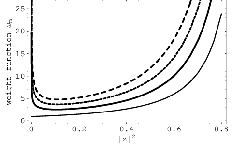
Figure 1: Plots of the weight function (IV.1.1) of the PA-SIPCS (94) versus |z|2|z|^{2} with |c|2=γ,|c|^{2}=\gamma, for different values of the photon added number mm with m=1m=1 (thin solid line), m=2m=2 (solid line), m=3m=3 (dot line), and m=4m=4 (dashed line).

Let us turn now to the problem of overcompleteness. The relation (48) gives in this D-type case:

∫0∞d​x​xn+m​gm​(x,ar)\displaystyle\int_{0}^{\infty}dx\ x^{n+m}\ g_{m}(x;a_{r}) =\displaystyle= |Knm​(ar)|2=γn​n!​Γ​(n+1)|c|2​n​γm​Γ​(n+m+1)\displaystyle|K_{n}^{m}(a_{r})|^{2}={\gamma^{n}n!\ \Gamma(n+1)\over|c|^{2n}\ \gamma^{m}\ \Gamma(n+m+1)} (101)

which, after performing the variable change n+m→s−1n+m\to s-1, leads to:

∫0∞d​x​xs−1​hm​(x,ar)\displaystyle\int_{0}^{\infty}dx\ x^{s-1}\ h_{m}(x;a_{r}) =\displaystyle= (|c|2γ)−s​(Γ⁡(s−m))2Γ⁡(s)\displaystyle\left(\displaystyle{|c|^{2}\over\gamma}\right)^{-s}{(\Gamma(s-m))^{2}\over\Gamma(s)} (102)

where hm​(x,ar)=gm​(x,ar)​γ2​m+1​c−2​(m+1)h_{m}(x;a_{r})=g_{m}(x;a_{r})\gamma^{2m+1}\ c^{-2(m+1)}. From the formula (III.3) of the Mellin-inversion theorem, we get:

hm​(x,ar)\displaystyle h_{m}(x;a_{r}) =\displaystyle= G1,22,0(|c|2γx|;0−m,−m;)\displaystyle G_{1,2}^{2,0}\left(\left.{|c|^{2}\over\gamma}x\right|\begin{array}[]{rcl}&;&0\\ -m,-m&;&\end{array}\right)

and the weight function gives

ωm(|z|2;ar)=1π|c|2γG1,21,1(−|c​z|2γ|−m;0;0)G1,22,0(|c|2γ|z|2|;m0,0;)\displaystyle\omega_{m}(|z|^{2};a_{r})={1\over\pi}{|c|^{2}\over\gamma}\,G_{1,2}^{1,1}\left(\left.-{|cz|^{2}\over\gamma}\right|\begin{array}[]{ccc}-m&;&\\ 0&;&0\end{array}\right)G_{1,2}^{2,0}\left(\left.{|c|^{2}\over\gamma}|z|^{2}\right|\begin{array}[]{rcl}&;&m\\ 0,0&;&\end{array}\right)

where we use (IV.1.1) and the multiplication formula of the Meijer’s G-function [36]

xαGm,np,q(x|(ap)(bq))=Gm,np,q(x|(ap+α)(bq+α)).\displaystyle x^{\alpha}G_{m,n}^{p,q}\left(x\left|\begin{array}[]{c}(a_{p})\\ (b_{q})\end{array}\right.\right)=G_{m,n}^{p,q}\left(x\left|\begin{array}[]{c}(a_{p}+\alpha)\\ (b_{q}+\alpha)\end{array}\right.\right).

Since the measure in equation (45) must be necessary positive, the function ωm​(|z|2,ar)\omega_{m}(|z|^{2};a_{r}) must be a positive function. This is confirmed in FIG. 1, where we represent the weight functions (IV.1.1) for m=1,2,3,4m=1,2,3,4. We can see that the weight function has a singularity at x=|z|2=0x=|z|^{2}=0 and tends to zero for x→∞x\to\infty. For m=0m=0, we recover the measure ω0​(|z|2,ar)=1π​|c|2γ\omega_{0}(|z|^{2};a_{r})=\displaystyle{1\over\pi}{|c|^{2}\over\gamma} obtained in [13]. Let us note that, by the variable change z→c​z/γz\to cz/\sqrt{\gamma}, we obtain, for m=0m=0, the bosonic coherent states of the harmonic oscillator [3]. Then, the PA-SIPCS (94) for |c|2=γ|c|^{2}=\gamma can be considered as the photon-added coherent states of the harmonic oscillator.
 

Refer to caption
Refer to caption
Figure 2: Plots of the Mandel Q-parameter (119)(a) and the second-order correlation function (120)(b) of the PA-SIPCS (94) versus |z|,|z|, for different values of the photon added number m,m, with m=1m=1 (thin solid line), m=2m=2 (solid line), m=5m=5 (dot line), and m=10m=10 (dashed line).

To finish with the D-type SI system, let us analyse the statistical properties of its PA-SIPCS states. Taking into account the expressions (84) and (87) of the factors Knm​(ar)K_{n}^{m}(a_{r}) and 𝒩m​(|z|2,ar){\cal N}_{m}(|z|^{2};a_{r}), the expectation values ⟨N⟩\left<N\right> and ⟨N2⟩\left<N^{2}\right> (72) are given by:

⟨N⟩\displaystyle\left<N\right> =\displaystyle= m​γ​F22​(m+1,m+1,1,m,|c​z|2/γ)F11​(m+1,1,|c​z|2/γ)\displaystyle m\gamma\ {{}_{2}F_{2}(m+1,m+1;1,m;|cz|^{2}/\gamma)\over{}_{1}F_{1}(m+1;1;|cz|^{2}/\gamma)} (116)
⟨N2⟩\displaystyle\left<N^{2}\right> =\displaystyle= m2​γ2​F33​(m+1,m+1,m+1,1,m,m,|c​z|2/γ)1F1(m+1;1;||cz|2/γ).\displaystyle m^{2}\gamma^{2}\ {{}_{3}F_{3}(m+1,m+1,m+1;1,m,m;|cz|^{2}/\gamma)\over{}_{1}F_{1}(m+1;1;||cz|^{2}/\gamma)}. (118)

Then, the Mandel Q-parameter and the second-order correlation function can be deduced, respectively, as:

Q=m​γ​(ℱ33​(|z|2,m,γ)ℱ22​(|z|2,m,γ)−ℱ22​(|z|2,m,γ)ℱ11​(|z|2,m,γ))−1,\displaystyle Q=m\gamma\left({{}_{3}{\cal F}_{3}(|z|^{2};m,\gamma)\over{}_{2}{\cal F}_{2}(|z|^{2};m,\gamma)}-{{}_{2}{\cal F}_{2}(|z|^{2};m,\gamma)\over{}_{1}{\cal F}_{1}(|z|^{2};m,\gamma)}\right)-1, (119)
g2=mγ3ℱ3(|z|2;m,γ)−2ℱ2(|z|2;m,γ)m​γ2​ℱ2​(|z|2,m,γ)​ℱ11​(|z|2,m,γ)ℱ22​(|z|2,m,γ),\displaystyle g^{2}={m\gamma\ _{3}{\cal F}_{3}(|z|^{2};m,\gamma)-_{2}{\cal F}_{2}(|z|^{2};m,\gamma)\over m\gamma\ _{2}{\cal F}_{2}(|z|^{2};m,\gamma)}\,{{}_{1}{\cal F}_{1}(|z|^{2};m,\gamma)\over{}_{2}{\cal F}_{2}(|z|^{2};m,\gamma)}, (120)

where ℱ11{}_{1}{\cal F}_{1}, ℱ22{}_{2}{\cal F}_{2} and ℱ33{}_{3}{\cal F}_{3} are the generalized hypergeometric functions:

ℱ11​(|z|2,m,γ){}_{1}{\cal F}_{1}(|z|^{2};m,\gamma) =\displaystyle= F11​(m+1,1,|c​z|2/γ){}_{1}F_{1}(m+1;1;|cz|^{2}/\gamma)
ℱ22​(|z|2,m,γ){}_{2}{\cal F}_{2}(|z|^{2};m,\gamma) =\displaystyle= F22​(m+1,m+1,1,m,|c​z|2/γ){}_{2}F_{2}(m+1,m+1;1,m;|cz|^{2}/\gamma)
ℱ33​(|z|2,m,γ){}_{3}{\cal F}_{3}(|z|^{2};m,\gamma) =\displaystyle= F33​(m+1,m+1,m+1,1,m,m,|c​z|2/γ).{}_{3}F_{3}(m+1,m+1,m+1;1,m,m;|cz|^{2}/\gamma).

The PND (68) reads as

𝒫n(m)​(|z|2,γ)=Γ⁡(n+1)Γ​(m+1)1​F1​(1+m,1,|c​z|2/γ)​(|c​z|2/γ)n−m((n−m)!)2\displaystyle{\cal P}_{n}^{(m)}(|z|^{2};\gamma)={\Gamma(n+1)\over\Gamma(m+1)\,_{1}F_{1}(1+m;1;|cz|^{2}/\gamma)}\,{(|cz|^{2}/\gamma)^{n-m}\over((n-m)!)^{2}} (121)

Refer to caption
Refer to caption
Figure 3: Plots of the photon number distribution (121) of the PA-SIPCS (94) versus the photon number nn for different values of the photon-added number mm for |z|=2|z|=2(a) and |z|=5|z|=5(b), respectively, with m=0m=0 (thin solid line), m=1m=1 (solid line), m=2m=2 (dot line) and m=3m=3 (dashed line).

In FIG. 2, the Mandel Q-parameter (119) and the second-order correlation function (120) derived for the PA-SIPCS (94) have been plotted in terms of the amplitude |z||z|, in (a) and (b), respectively, for different values of the photon-added number mm, where |c|2=γ|c|^{2}=\gamma. As shown in FIG. 2, the number mm increases as the Mandel Q-parameter decreases, while the second-order correlation function increases. In addition, the Mandel Q-parameter increasing, takes negative values for given |z||z| and mm and asymptotically tends to 00. As for the second-order correlation function, it increases and asymptotically tends to 11. This indicates that the PA-SIPCS obey sub-Poissonian distribution statistics. Hence, for larger z,z, the PA-SIPCS (94) behave like the states exhibiting Poissonian statistics.
In FIG. 3, the PND of the PA-SIPCS (94), as a function of |z||z|, is depicted in (a) and (b) for |z|=2|z|=2 and |z|=5,|z|=5, respectively, with different values of the photon-added number mm. As |z||z| and mm increase, the peaks decrease and shift to the right.

IV.1.2 C-Type shape invariant systems

For C-type systems, we consider the auxiliary function [13]:

g⁡(aj,c,d)\displaystyle g(a_{j};c,d) =\displaystyle= c​aj+d\displaystyle ca_{j}+d (122)

where cc and dd are constants. Using the potential parameter relations (IV.1), we can obtain, after a straightforward computation, that:

∏k=mn+m−1g⁡(aj,c,d)=(−c)n​Γ⁡(n+m−a1+j−1−dc)Γ⁡(m−a1+j−1−dc).\displaystyle\prod_{k=m}^{n+m-1}g(a_{j};c,d)=(-c)^{n}{\Gamma\left(n+m-a_{1}+j-1-{d\over c}\right)\over\Gamma\left(m-a_{1}+j-1-{d\over c}\right)}. (123)

Defining the functional 𝒵j:=g⁡(a1,−γ,1)​e−i​α​ℛ​(a1){\cal Z}_{j}:=\sqrt{g(a_{1};-\gamma,1)}\,e^{-i\alpha{\cal R}(a_{1})}, we get:

∏k=mn+m−1Zj+k=γn​Γ​(−ρ+m+n)Γ⁡(−ρ+m)​e−i​α​n​γ\displaystyle\prod_{k=m}^{n+m-1}Z_{j+k}=\sqrt{\gamma^{n}\Gamma(-\rho+m+n)\over\Gamma(-\rho+m)}\,e^{-i\alpha n\gamma} (124)

where we set ρ=a1−1γ\rho=a_{1}-{1\over\gamma}. This last relation, with (82) inserted in (37), gives for C-Type systems:

Knm​(ar)\displaystyle K_{n}^{m}(a_{r}) =\displaystyle= [Γ⁡(−ρ+m)​Γ​(n+1)2γm​Γ​(−ρ+m+n)​Γ​(n+m+1)]1/2​ei​α​n​γ.\displaystyle\left[{\Gamma(-\rho+m)\Gamma(n+1)^{2}\over\gamma^{m}\Gamma(-\rho+m+n)\Gamma(n+m+1)}\right]^{1/2}\ e^{i\alpha n\gamma}. (125)

The normalized form of the C-type PA-SIPCS, defined on the unit open disc |z|<1|z|<1, can be written as:

|z;ar⟩m=𝒩m(|z|2;ar)∑n=0∞γm​Γ​(−ρ+m+n)​Γ​(n+m+1)Γ⁡(−ρ+m)e−i​α​n​γznn!|Ψn+m⟩\displaystyle\left|z;a_{r}\right>_{m}={\cal N}_{m}(|z|^{2};a_{r})\sum_{n=0}^{\infty}\sqrt{\displaystyle{\gamma^{m}\Gamma(-\rho+m+n)\Gamma(n+m+1)\over\Gamma(-\rho+m)}}\,e^{-i\alpha n\gamma}\ {z^{n}\over n!}\left|\Psi_{n+m}\right> (126)

where the normalization factor is given by:

𝒩m​(|z|2,ar)\displaystyle{\cal N}_{m}(|z|^{2};a_{r}) =\displaystyle= [γmΓ(m+1)2F1(m−ρ,m+1;1;|z|2)]−1/2.\displaystyle\left[\gamma^{m}\ \Gamma(m+1)\ _{2}F_{1}\left(m-\rho,m+1;1;|z|^{2}\right)\right]^{-1/2}. (127)

Using Eq. (IV.1.1), the normalization factor can also be formulated in terms of Meijer’s G-function as:

𝒩m​(|z|2,ar)\displaystyle{\cal N}_{m}(|z|^{2};a_{r}) =\displaystyle= [γmΓ⁡(m−ρ)G2,21,2(−|z|2|−m,1−m+ρ;0;0)]−1/2.\displaystyle\left[{\gamma^{m}\over\Gamma(m-\rho)}\ G_{2,2}^{1,2}\left(-|z|^{2}\left|\begin{array}[]{ccc}-m,1-m+\rho&;&\\ 0&;&0\end{array}\right.\right)\right]^{-1/2}.

For m=0m=0, Knm​(ar)K_{n}^{m}(a_{r}) and 𝒩m​(|z|2,ar){\cal N}_{m}(|z|^{2};a_{r}) reduce to the equivalent quantities hn​(ar)h_{n}(a_{r}) and 𝒩⁡(|z|2,ar){\cal N}(|z|^{2};a_{r}), respectively, for the corresponding ordinary SIPCS [13] :

Kn0​(ar)\displaystyle K_{n}^{0}(a_{r}) =\displaystyle= Γ⁡(−ρ)​Γ​(n+1)Γ⁡(n−ρ)​ei​α​n​γ=hn​(ar)\displaystyle\sqrt{\Gamma(-\rho)\Gamma(n+1)\over\Gamma(n-\rho)}\,e^{i\alpha n\gamma}=h_{n}(a_{r}) (131)
𝒩0​(|z|2,ar)\displaystyle{\cal N}_{0}(|z|^{2};a_{r}) =\displaystyle= (1−|z|2)−ρ/2=𝒩(|z|2;ar).\displaystyle(1-|z|^{2})^{-\rho/2}={\cal N}(|z|^{2};a_{r}). (132)

Then, the PA-SIPCS correspond to ordinary SIPCS obtained in [13] :

|z;ar⟩=(1−|z|2)−ρ/2∑n=0∞Γ⁡(n−ρ)Γ⁡(−ρ)​Γ​(n+1)e−i​α​n​γzn|Ψn⟩\displaystyle\left|z;a_{r}\right>=(1-|z|^{2})^{-\rho/2}\sum_{n=0}^{\infty}\sqrt{\Gamma(n-\rho)\over\Gamma(-\rho)\Gamma(n+1)}\,e^{-i\alpha n\gamma}\,z^{n}\left|\Psi_{n}\right> (133)

which are the Perelomov CS for the SU(1,1) group [9]. Consequently, Eqs. (126) and (127) can be considered as the PA-SIPCS associated to the Perelomov CS.
The inner product of two different PA-SIPCS |z;ar⟩m\left|z;a_{r}\right>_{m} and |z′;ar⟩m′\left|z^{\prime};a_{r}\right>_{m^{\prime}} follows from Eq (42):

⟨z′;ar|z;ar⟩mm′=F(ρ,m,m′)2F1(m−ρ,m+1;m−m′+1;z′⋆z){}_{m^{\prime}}\left<z^{\prime};a_{r}\right|\left.z;a_{r}\right>_{m}=F(\rho,m,m^{\prime})\ _{2}F_{1}(m-\rho,m+1;m-m^{\prime}+1;{z^{\prime}}^{\star}z) (134)

where

F⁡(ρ,m,m′)=𝒩m′​(|z′|2,ar)​𝒩m​(|z|2,ar)​Γ⁡(m+1)Γ⁡(m−m′+1)​γ(m+m′)​Γ​(−ρ+m)¯​Γ​(−ρ+m′)​ei​α​(m−m′)​γ.\displaystyle F(\rho,m,m^{\prime})={\cal N}_{m^{\prime}}(|z^{\prime}|^{2};a_{r})\ {\cal N}_{m}(|z|^{2};a_{r})\ {\Gamma(m+1)\over\Gamma(m-m^{\prime}+1)}\ \sqrt{\gamma^{(m+m^{\prime})}\Gamma(-\rho+m)\over\textasciimacron\Gamma(-\rho+m^{\prime})}\ e^{i\alpha(m-m^{\prime})\gamma}. (135)

For m=m′=0m=m^{\prime}=0, we recover the result for the SIPCS obtained in [13]:

⟨z′;ar|z;ar⟩00{}_{0}\left<z^{\prime};a_{r}\right|\left.z;a_{r}\right>_{0} =\displaystyle= 𝒩⁡(|z′|2,ar)​𝒩​(|z|2,ar)2​F1​(−ρ,1,1,z′⁣⋆​z)=[(1−|z|2)​(1−|z′|2)1−z′⁣⋆​z]−ρ.\displaystyle{\cal N}(|z^{\prime}|^{2};a_{r}){\cal N}(|z|^{2};a_{r})_{2}F_{1}(-\rho,1;1;{z^{\prime\star}}z)=\left[{\sqrt{(1-|z|^{2})(1-|z^{\prime}|^{2})}\over 1-{z^{\prime\star}}z}\right]^{-\rho}. (136)
Refer to caption
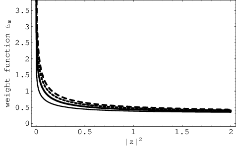
Figure 4: Plots of the weight function (IV.1.2) of the PA-SIPCS (126) versus |z|2|z|^{2} for different values of the photon added number mm with m=0m=0 (thin solid line), m=1m=1 (solid line), m=2m=2 (dot line), and m=3m=3 (dashed line).

Taking into account the expression (125) of the expansion coefficient, the overcompleteness relation (48) becomes

∫0∞d​x​xn+m​gm​(x,ar)=Γ⁡(−ρ+m)​Γ​(n+1)​Γ​(n+1)γm​Γ​(−ρ+m+n)​Γ​(n+m+1).\displaystyle\int_{0}^{\infty}dx\ x^{n+m}g_{m}(x;a_{r})={\Gamma(-\rho+m)\Gamma(n+1)\Gamma(n+1)\over\gamma^{m}\Gamma(-\rho+m+n)\Gamma(n+m+1)}. (137)

Making the variable change n+m→s−1n+m\to s-1, we get

∫0∞d​x​xs−1​hm​(x,ar)=Γ⁡(s−m)​Γ​(s−m)Γ⁡(s)​Γ​(s−ρ−1)\displaystyle\int_{0}^{\infty}dx\ x^{s-1}\ h_{m}(x;a_{r})={\Gamma(s-m)\Gamma(s-m)\over\Gamma(s)\Gamma(s-\rho-1)} (138)

where hm=γmΓ⁡(−ρ+m)×gmh_{m}=\displaystyle{\gamma^{m}\over\Gamma(-\rho+m)}\times g_{m}. Identifying Eq. (138) and taking into account the formuula (III.3) given by the Mellin inversion theorem, we deduce

hm=G2,22,0(|z|2|;0,−ρ−1−m,−m;).\displaystyle h_{m}=G_{2,2}^{2,0}\left(\left.|z|^{2}\right|\begin{array}[]{rcl}&;&0,-\rho-1\\ -m,-m&;&\end{array}\right).

Then the measure is derived as

ωm​(|z|2;arCLOSE\displaystyle\omega_{m}(|z|^{2};a_{r} =\displaystyle= 1πG2,21,2(−|z|2|−m,1−m+ρ;0;0)G2,22,0(|z|2|;m,m−ρ−10,0;)\displaystyle{1\over\pi}G_{2,2}^{1,2}\left(-|z|^{2}\left|\begin{array}[]{ccc}-m,1-m+\rho&;&\\ 0&;&0\end{array}\right.\right)G_{2,2}^{2,0}\left(|z|^{2}\left|\begin{array}[]{rcl}&;&m,m-\rho-1\\ 0,0&;&\end{array}\right.\right)

where we use (IV.1.2) and the multiplication formula of the Meijer’s G-function (IV.1.1). The measure (IV.1.2) is positive for ρ<−1\rho<-1 as shown on the representation in FIG. 4. for ρ=−2\rho=-2 and for m=0,1,2,3m=0,1,2,3. We remark that the measure ωm​(|z|2,ar)\omega_{m}(|z|^{2};a_{r}) for m≠0m\neq 0 has the same behaviour as the measure corresponding to the conventional coherent states (m=0m=0). It presents singularities at x=0x=0 and x=1x=1. For m=0m=0, the Meijer’s G-function reduces to (1−|z|2)−ρ−2Γ⁡(−ρ−1)\displaystyle{(1-|z|^{2})^{-\rho-2}\over\Gamma(-\rho-1)} and we recover the measure −1π​(1+ρ)​(1−|z|2)−2-{1\over\pi}(1+\rho)(1-|z|^{2})^{-2} obtained in [13].  

Refer to caption
Refer to caption
Figure 5: Plots of the Mandel Q-parameter (149)(a) and the second-order correlation function (150)(b) of the PA-SIPCS (126) versus |z||z| with the parameter ρ=−4\rho=-4 for different values of the photon added number mm with m=1m=1 (thin solid line), m=2m=2 (solid line), m=5m=5 (dot line), and m=10m=10 (dashed line).

We end the discussion on C-type SI systems by the study of the statistical properties of their PA-SIPCS states. Inserting the expressions (125) and (127) of the factors Knm​(ar)K_{n}^{m}(a_{r}) and 𝒩m​(|z|2,ar){\cal N}_{m}(|z|^{2};a_{r}) in Eq. (72), we obtain the expectation values of ⟨N⟩\left<N\right> and ⟨N2⟩\left<N^{2}\right> as:

⟨N⟩\displaystyle\left<N\right> =\displaystyle= m​γ​F23​(−ρ+m,m+1,m+1,1,m,|z|2)F12​(−ρ+m,m+1,1,|z|2)\displaystyle m\gamma\ {{}_{3}F_{2}(-\rho+m,m+1,m+1;1,m;|z|^{2})\over{}_{2}F_{1}(-\rho+m,m+1;1;|z|^{2})} (147)
⟨N2⟩\displaystyle\left<N^{2}\right> =\displaystyle= m2​γ2​F34​(−ρ+m,m+1,m+1,m+1,1,m,m,|z|2)F12​(−ρ+m,m+1,1,|z|2).\displaystyle m^{2}\gamma^{2}\ {{}_{4}F_{3}(-\rho+m,m+1,m+1,m+1;1,m,m;|z|^{2})\over{}_{2}F_{1}(-\rho+m,m+1;1;|z|^{2})}. (148)

Then, the Mandel Q-parameter and the second-order correlation function can be deduced, respectively, as:

Q=m​γ​(ℱ34​(|z|2,m,ρ)ℱ23​(|z|2,m,ρ)−ℱ23​(|z|2,m,ρ)ℱ12​(|z|2,m,ρ))−1\displaystyle Q=m\gamma\left({{}_{4}{\cal F}_{3}(|z|^{2};m,\rho)\over{}_{3}{\cal F}_{2}(|z|^{2};m,\rho)}-{{}_{3}{\cal F}_{2}(|z|^{2};m,\rho)\over{}_{2}{\cal F}_{1}(|z|^{2};m,\rho)}\right)-1 (149)
g2=mγ4ℱ3(|z|2;m,ρ)−3ℱ2(|z|2;m,ρ)m​γ3​ℱ2​(|z|2,m,ρ)​ℱ12​(|z|2,m,ρ)ℱ23​(|z|2,m,ρ),\displaystyle g^{2}={m\gamma\ _{4}{\cal F}_{3}(|z|^{2};m,\rho)-_{3}{\cal F}_{2}(|z|^{2};m,\rho)\over m\gamma\ _{3}{\cal F}_{2}(|z|^{2};m,\rho)}\,{{}_{2}{\cal F}_{1}(|z|^{2};m,\rho)\over{}_{3}{\cal F}_{2}(|z|^{2};m,\rho)}, (150)

where ℱ12{}_{2}{\cal F}_{1}, ℱ23{}_{3}{\cal F}_{2} and ℱ34{}_{4}{\cal F}_{3} are the generalized hypergeometric functions:

ℱ12​(|z|2,m,ρ){}_{2}{\cal F}_{1}(|z|^{2};m,\rho) =\displaystyle= F12​(−ρ+m,m+1,1,|z|2){}_{2}F_{1}(-\rho+m,m+1;1;|z|^{2})
ℱ23​(|z|2,m,ρ){}_{3}{\cal F}_{2}(|z|^{2};m,\rho) =\displaystyle= F23​(−ρ+m,m+1,m+1,1,m,|z|2){}_{3}F_{2}(-\rho+m,m+1,m+1;1,m;|z|^{2})
ℱ34​(|z|2,m,ρ){}_{4}{\cal F}_{3}(|z|^{2};m,\rho) =\displaystyle= F34​(−ρ+m,m+1,m+1,m+1,1,m,m,|z|2).{}_{4}F_{3}(-\rho+m,m+1,m+1,m+1;1,m,m;|z|^{2}).
Refer to caption
Refer to caption
Figure 6: Plots of the photon number dstribution (121) of the PA-SIPCS (126) versus the photon number nn for different values of the photon-added number mm with parameter ρ=−8\rho=-8 for |z|=0.5|z|=0.5(a) and |z|=0.8|z|=0.8(b), respectively, with m=0m=0 (thin solid line), m=1m=1 (solid line), m=2m=2 (dot line) and m=3m=3 (dashed line).

The PND (68) reads as

𝒫n(m)​(|z|2,ρ)=Γ⁡(n+1)​Γ​(n−ρ)Γ⁡(m−ρ)​Γ​(m+1)2​ℱ1​(|z|2,m,ρ)​(|z|)2​(n−m)((n−m)!)2.\displaystyle{\cal P}_{n}^{(m)}(|z|^{2};\rho)={\Gamma(n+1)\Gamma(n-\rho)\over\Gamma(m-\rho)\Gamma(m+1)\,_{2}{\cal F}_{1}(|z|^{2};m,\rho)}\,{(|z|)^{2(n-m)}\over((n-m)!)^{2}}. (151)

In FIG. 5, the Mandel Q-parameter (149) and the second-order correlation function (150) derived in the PA-SIPCS (126) are plotted in terms of the amplitude |z||z|, in (a) and (b), respectively, for different values of the photon-added number mm with the potential parameter ρ=−4\rho=-4. As |z||z| increases from 00 to 11, the Mandel Q-parameter increases from negative values to positive ones, while the second-order correlation function increases from g2<1g^{2}<1 to g2>1g^{2}>1. Thus, there exists a value z0z_{0}, depending on the parameter ρ\rho, such that the PASIPCS (126) exhibit sub-Poisonnian distribution for 0<|z|<|z0|0<|z|<|z_{0}|, Poissonian for |z|=|z0||z|=|z_{0}| and super-Poisonnian distribution for |z0|<|z|<1|z_{0}|<|z|<1.
In FIG. 6, the PND obtained in the PA-SIPCS (126) as a function of |z||z|, is depicted in (a) and (b) for |z|=0.5|z|=0.5 and |z|=0.8|z|=0.8, respectively, for different values of the photon-added number mm. Increasing the number mm shifts the PND. The peaks position increases with the photon-added number mm and the amplitude |z||z|, while their intensities decrease.

IV.2 Type A and B SIP systems

The superpotentials for these types of SI systems are:

WA​(x,a1)\displaystyle W_{A}(x;a_{1}) =\displaystyle= β⁡(a1+γ)​cot⁡[u⁡(x)]+δsin⁡[u⁡(x)],u⁡(x)≡β⁡(x+λ)\displaystyle\beta(a_{1}+\gamma)\cot[u(x)]+{\delta\over\sin[u(x)]},\quad u(x)\equiv\beta(x+\lambda) (152)
WB​(x,a1)\displaystyle W_{B}(x;a_{1}) =\displaystyle= i​β​(a1+γ)+δ​e−i​β​x\displaystyle i\beta(a_{1}+\gamma)+\delta e^{-i\beta x} (153)

where β\beta is a real constant for A-type or pure imaginary for B-type and γ,λ,δ\gamma,\lambda,\delta are real constants. For both cases, the remainder in the shape invariant condition (13) is ℛ⁡(a1)=β2​[2​(a1+γ)−1]{\cal R}(a_{1})=\beta^{2}[2(a_{1}+\gamma)-1], the potential parameters being related as: an+1=an−1a_{n+1}=a_{n}-1. Since we are interested to bound states Hamiltonian, we restrict our attention to A-type systems. For these systems, the products in terms of the quantity ℛ⁡(as){\cal R}(a_{s}) in the numerator and denominator of the coefficient Knm​(ar)K_{n}^{m}(a_{r}), see Eq. (37), can be read, respectively, as:

∏k=m+1n+m(∑s=kn+mℛ⁡(as))\displaystyle\prod_{k=m+1}^{n+m}\left(\sum_{s=k}^{n+m}{\cal R}(a_{s})\right) =\displaystyle= β2​n​Γ⁡(n+1)​Γ​(2​n+2​m+2​ρ)Γ⁡(n+2​m+2​ρ)\displaystyle\beta^{2n}\frac{\Gamma(n+1)\Gamma(2n+2m+2\rho)}{\Gamma(n+2m+2\rho)} (154)
∏k=1m(∑s=kn+mℛ⁡(as))\displaystyle\prod_{k=1}^{m}\left(\sum_{s=k}^{n+m}{\cal R}(a_{s})\right) =\displaystyle= β2​m​Γ⁡(n+m+1)​Γ​(n+2​m+2​ρ)Γ⁡(n+1)​Γ​(n+m+2​ρ)\displaystyle\beta^{2m}\frac{\Gamma(n+m+1)\Gamma(n+2m+2\rho)}{\Gamma(n+1)\Gamma(n+m+2\rho)} (155)

where we set ρ=−(a1+γ)\rho=-(a_{1}+\gamma). The explicit form of the expansion coefficient Knm​(ar)K_{n}^{m}(a_{r}) depends on the choice of the functional 𝒵j{\cal Z}_{j}. We adopt the functionals used in [13] for commodity of comparison.

IV.2.1 First choice of the functional 𝒵j{\cal Z}_{j}

First we make the choice 𝒵j=c{\cal Z}_{j}=c, where cc is a real constant. Then ∏k=mn+m−1𝒵j+k=cn\displaystyle\prod_{k=m}^{n+m-1}{{\cal Z}_{j+k}}=c^{n}. Inserting this and the results (154) and (155) in (37), we obtain the expansion coefficient as:

Knm​(ar)\displaystyle K_{n}^{m}(a_{r}) =\displaystyle= 1κm​Γ​(n+1)2​Γ​(2​n+2​m+2​ρ)​Γ​(n+m+2​ρ)Γ⁡(n+m+1)​Γ​(n+2​m+2​ρ)2\displaystyle{1\over\kappa^{m}}\ \sqrt{\frac{\Gamma(n+1)^{2}\ \Gamma(2n+2m+2\rho)\ \Gamma(n+m+2\rho)}{\Gamma(n+m+1)\Gamma(n+2m+2\rho)^{2}}} (156)

where we set κ=β=c\kappa=\beta=c.
(i) Normalization
The normalization factor, in terms of the generalized hypergeometric functions F43{}_{3}F_{4}, can readily be deduced from the above relation as:

𝒩m​(|z|2,ar)\displaystyle{\cal N}_{m}(|z|^{2};a_{r}) =\displaystyle= [ξ(m,ρ)F43(m+1,2m+2ρ,2m+2ρ;1,m+ρ,m+2ρ,m+ρ+1/2;|z|24)]−1/2\displaystyle\left[\xi(m,\rho){}_{3}F_{4}\left(m+1,2m+2\rho,2m+2\rho;1,m+\rho,m+2\rho,m+\rho+1/2;{|z|^{2}\over 4}\right)\right]^{-1/2} (157)

where ξ⁡(m,ρ)=κ2​m​Γ​(m+1)​Γ​(2​m+2​ρ)Γ⁡(m+2​ρ)\xi(m,\rho)=\displaystyle{\kappa^{2m}\Gamma(m+1)\Gamma(2m+2\rho)\over\Gamma(m+2\rho)}. In terms of Meijer’s G-function, we have:

𝒩m​(|z|2,ar)\displaystyle{\cal N}_{m}(|z|^{2};a_{r}) =\displaystyle= [χ(m,ρ)G3,51,3(−|z|24|−m,1−2​m−2​ρ,1−2​m−2​ρ;0,0,1−m−ρ,1−m−2​ρ,1/2−m−ρ)]−1/2\displaystyle\left[\chi(m,\rho)\ G_{3,5}^{1,3}\left(-{|z|^{2}\over 4}\left|\begin{array}[]{l}-m,1-2m-2\rho,1-2m-2\rho;\\ 0,0,1-m-\rho,1-m-2\rho,1/2-m-\rho\end{array}\right.\right)\right]^{-1/2}

with χ⁡(m,ρ)=κ2​m​Γ​(m+ρ)​Γ​(m+ρ+12)Γ⁡(2​m+2​ρ)\chi(m,\rho)=\displaystyle{\kappa^{2m}\Gamma(m+\rho)\Gamma(m+\rho+\mbox{\small{$\frac{1}{2}$}})\over\Gamma(2m+2\rho)} and where we use the more compact notation of Meijer’s G-function.

Gp,qm,n(x|a1,…,apb1,…,bq).\displaystyle G_{p,q}^{m,n}\left(x\left|\begin{array}[]{c}a_{1},...,a_{p}\\ b_{1},...,b_{q}\end{array}\right.\right).

The explicit form of the PA-SIPCS are:

|z;ar⟩m=𝒩m(|z|2;ar)κm∑n=0∞Γ⁡(n+m+1)​Γ​(n+2​m+2​ρ)2Γ⁡(n+m+2​ρ)​Γ​(2​n+2​m+2​ρ)znn!|n+m⟩\displaystyle\left|z;a_{r}\right>_{m}={\cal N}_{m}(|z|^{2};a_{r})\kappa^{m}\sum_{n=0}^{\infty}\sqrt{\frac{\Gamma(n+m+1)\Gamma(n+2m+2\rho)^{2}}{\Gamma(n+m+2\rho)\Gamma(2n+2m+2\rho)}}\,{z^{n}\over n!}\left|n+m\right> (164)

defined on the whole complex plane. For m=0m=0, we recover the expansion coefficient and the normalization factor obtained in [13] for the generalized SIPCS:

Kn0\displaystyle K_{n}^{0} =\displaystyle= Γ⁡(n+1)​Γ​(2​ρ+2​n)Γ⁡(2​ρ+n)=hn​(ar),\displaystyle\sqrt{\Gamma(n+1)\Gamma(2\rho+2n)\over\Gamma(2\rho+n)}=h_{n}(a_{r}), (165)
𝒩0​(|z|2,ar)\displaystyle{\cal N}_{0}(|z|^{2};a_{r}) =\displaystyle= [F21(2ρ;ρ,ρ+1/2;|z|24)]−1/2=𝒩(|z|2;ar).\displaystyle\left[{}_{1}F_{2}\left(2\rho;\rho,\rho+1/2;{|z|^{2}\over 4}\right)\right]^{-1/2}={\cal N}(|z|^{2};a_{r}). (166)

For giving mm, fixing ρ=1/2\rho=1/2, the states (164) become

|z;ar⟩m=𝒩m(|z|2;ar)κm∑n=0∞(n+2​m)2!(2​n+2​m)!znn!|n+m⟩\displaystyle\left|z;a_{r}\right>_{m}={\cal N}_{m}(|z|^{2};a_{r})\kappa^{m}\sum_{n=0}^{\infty}\sqrt{\frac{(n+2m)^{2}!}{(2n+2m)!}}{z^{n}\over n!}\,\left|n+m\right> (167)

with

𝒩m(|z|2;ar)=[κ2​mΓ(2m+1)F32(2m+1,2m+1;1,m+1,m+1/2;|z|24)]−1/2.\displaystyle{\cal N}_{m}(|z|^{2};a_{r})=\left[\kappa^{2m}\Gamma(2m+1){}_{2}F_{3}\left(2m+1,2m+1;1,m+1,m+1/2;{|z|^{2}\over 4}\right)\right]^{-1/2}.

Setting m=0m=0 in (167), we recover the ordinary SIPCS obtained in [12]:

|z;ar⟩=sech​(|z|)∑n=0∞zn2​n!|n⟩.\displaystyle\left|z;a_{r}\right>=\sqrt{{\textrm{sech}}(|z|)}\,\sum_{n=0}^{\infty}{z^{n}\over\sqrt{2n!}}\,\left|n\right>. (168)

(ii) Non-orthogonality
The inner product of two different PA-SIPCS |z;ar⟩m\left|z;a_{r}\right>_{m} and |z′;ar⟩m′\left|z^{\prime};a_{r}\right>_{m^{\prime}} follows from Eq (42):

⟨z′;ar|z;ar⟩mm′=χ(z′,z,m,m′,ρ)×{}_{m^{\prime}}\left<z^{\prime};a_{r}\right|\left.z;a_{r}\right>_{m}=\chi(z^{\prime},z,m,m^{\prime},\rho)\times
×3F4(m+1,2m+2ρ,m+m′+2ρ;m−m′+1,m+2ρ,m+ρ,m+ρ+12;z′⋆​z4)\displaystyle\times_{3}F_{4}\left(m+1,2m+2\rho,m+m^{\prime}+2\rho;m-m^{\prime}+1,m+2\rho,m+\rho,m+\rho+\mbox{\small{$\frac{1}{2}$}};{{z^{\prime}}^{\star}z\over 4}\right)

where

χ⁡(z′,z,m,m′,ρ)=𝒩m′​(|z′|2,ar)​𝒩m​(|z|2,ar)​z′⋆(m−m′)​κ(m+m′)​Γ⁡(m+1)​Γ​(m+m′+2​ρ)Γ⁡(m−m′+1)​Γ​(m+2​ρ).\displaystyle\chi(z^{\prime},z,m,m^{\prime},\rho)={\cal N}_{m^{\prime}}(|z^{\prime}|^{2};a_{r})\ {\cal N}_{m}(|z|^{2};a_{r})\ {{z^{\prime}}^{\star}}^{(m-m^{\prime})}\kappa^{(m+m^{\prime})}{\Gamma(m+1)\Gamma(m+m^{\prime}+2\rho)\over\Gamma(m-m^{\prime}+1)\Gamma(m+2\rho)}.
Refer to caption
Figure 7: Plots of the weight function (IV.2.1) of the PA-SIPCS (164) versus |z|2|z|^{2} for different values of the photon added number mm with m=0m=0 (thin solid line), m=m= (solid line), m=3m=3 (dot line), and m=4m=4 (dashed line).

(iii) Overcompleteness
The non-negative weight function ωm​(|z|2,ar)\omega_{m}(|z|^{2};a_{r}) is related to the function gmg_{m} satisfying (48):

∫0∞d​x​xn+m​gm​(x,ar)\displaystyle\int_{0}^{\infty}dx\,x^{n+m}\,g_{m}(x;a_{r}) =\displaystyle= ξ⁡(x,n,m,ρ)\displaystyle\xi(x,n,m,\rho)\, (170)
×Γ​(n+1)2​Γ​(n+m+2​ρ)​Γ​(n+m+ρ)​Γ​(n+m+ρ+12)Γ⁡(n+m+1)​Γ​(n+2​m+2​ρ)2\displaystyle\times{\Gamma(n+1)^{2}\Gamma(n+m+2\rho)\Gamma(n+m+\rho)\Gamma(n+m+\rho+\mbox{\small{$\frac{1}{2}$}})\over\Gamma(n+m+1)\Gamma(n+2m+2\rho)^{2}}

where xx stands for |z|2|z|^{2}, ξ⁡(x,n,m,ρ)=2(2​n+2​m+2​ρ)2​π​κ2​m\xi(x,n,m,\rho)=\displaystyle{2^{(2n+2m+2\rho)}\over 2\sqrt{\pi}\kappa^{2m}} and ωm=xm​gm​(x,ar)π​Nm2​(x,ar)\omega_{m}=\displaystyle{x^{m}g_{m}(x;a_{r})\over\pi N_{m}^{2}(x;a_{r})}. After variable change n+m→s−1n+m\to s-1, (170) becomes

∫0∞d​x​xs−1​hm​(x,ar)=(14)−s​Γ​(s−m)2​Γ​(s−1+2​ρ)​Γ​(s−1+ρ)​Γ​(s−1/2+ρ)Γ⁡(s)​Γ​(s−1+2​ρ+m)2\displaystyle\int_{0}^{\infty}dx\,x^{s-1}\,h_{m}(x;a_{r})=\left({1\over 4}\right)^{-s}\,{\Gamma(s-m)^{2}\Gamma(s-1+2\rho)\Gamma(s-1+\rho)\Gamma(s-1/2+\rho)\over\Gamma(s)\Gamma(s-1+2\rho+m)^{2}} (171)

where hm​(x,ar)h_{m}(x;a_{r}) is related to gm​(x,ar)g_{m}(x;a_{r}) as: gm=12​π​κ−2​m​22​(ρ−1)​hm​(x,ar)g_{m}={1\over 2\sqrt{\pi}}\kappa^{-2m}2^{2(\rho-1)}h_{m}(x;a_{r}). Then, using the Mellin inversion theorem in terms of Meijer’s G-function (III.3), we deduce:

ωm​(|z|2,ar)\displaystyle\omega_{m}(|z|^{2};a_{r}) =\displaystyle= 14​πG3,51,3(−|z|24|−m,1−2​m−2​ρ,1−2​m−2​ρ;0,0,1−m−ρ,1−m−2​ρ,1/2−m−ρ)×\displaystyle{1\over 4\pi}G_{3,5}^{1,3}\left(-{|z|^{2}\over 4}\left|\begin{array}[]{l}-m,1-2m-2\rho,1-2m-2\rho;\\ 0,0,1-m-\rho,1-m-2\rho,1/2-m-\rho\end{array}\right.\right)\times
×G3,55,0(|z|24|m,−1+2​ρ+2​m,−1+2​ρ+2​m0,0,2ρ+m−1,−1+m+ρ,−1/2+m+ρ)\displaystyle\times G_{3,5}^{5,0}\left({|z|^{2}\over 4}\left|\begin{array}[]{l}m,-1+2\rho+2m,-1+2\rho+2m\\ 0,0,2\rho+m-1,-1+m+\rho,-1/2+m+\rho\end{array}\right.\right)

where we use (IV.2.1). The weight function (IV.2.1) is positive for the parameter ρ>0\rho>0 as confirmed in FIG. 7, where the curves are represented for ρ=12\rho=\mbox{\small{$\frac{1}{2}$}} and for m=0,1,2,3m=0,1,2,3. All the functions are positive for x=|z|2∈I​R+x=|z|^{2}\in\rm I\!R_{+} and tend asymptotically to the measure of the conventional CS (m=0)(m=0). The measure has a singularity at x=0x=0 and tends to zero for x→∞.x\to\infty. For m=0m=0 and ρ=1/2\rho=1/2 we have h0=2​π​e−|z||z|h_{0}=\displaystyle 2\sqrt{\pi}{e^{-|z|}\over|z|} and 𝒩02​(|z|2,ar)=sech​(|z|){\cal N}_{0}^{2}(|z|^{2};a_{r})={\textrm{sech}}(|z|). Then, we recover the weight function ω⁡(|z|2,ar)=cosh⁡(|z|)π​e−|z|2​|z|\omega(|z|^{2};a_{r})=\displaystyle{\cosh(|z|)\over\pi}{e^{-|z|}\over 2|z|} obtained in [12].
(iv) Statistical properties

Refer to caption
Refer to caption
Figure 8: Plots of the Mandel Q-parameter (179)(a) and the second-order correlation function (180)(b) of the PA-SIPCS (164) versus |z||z| with the parameter ρ=12\rho=\mbox{\small{$\frac{1}{2}$}} for different values of the photon added number mm with m=1m=1 (thin solid line), m=2m=2 (solid line), m=5m=5 (dot line), and m=10m=10 (dashed line).

We consider now the statistical properties of the state (164). The expectation values ⟨H⟩\left<H\right> and ⟨H2⟩\left<H^{2}\right> result from the expressions (156) and (157) of KnmK_{n}^{m} and 𝒩m{\cal N}_{m}, respectively, as:

⟨N⟩\displaystyle\left<N\right> =\displaystyle= κ2​m​(m+2​ρ)​ℱ65​(|z|2,m,ρ)ℱ3​4​(|z|2,m,ρ),⟨N2⟩=κ4​m2​(m+2​ρ)2​ℱ87​(|z|2,m,ρ)ℱ43​(|z|2,m,ρ).\displaystyle\kappa^{2}m(m+2\rho){{}_{5}{\cal F}_{6}(|z|^{2};m,\rho)\over{}_{3}{\cal F}4(|z|^{2};m,\rho)}\hskip 9.24994pt,\hskip 9.24994pt\left<N^{2}\right>=\kappa^{4}m^{2}(m+2\rho)^{2}{{}_{7}{\cal F}_{8}(|z|^{2};m,\rho)\over{}_{3}{\cal F}_{4}(|z|^{2};m,\rho)}. (178)

Then, the Mandel Q-parameter and the second-order correlation function are derived, respectively, as:

Q\displaystyle Q =\displaystyle= κ2​m​(m+2​ρ)​(ℱ87​(|z|2,m,ρ)ℱ65​(|z|2,m,ρ)−ℱ65​(|z|2,m,ρ)ℱ43​(|z|2,m,ρ))−1\displaystyle\kappa^{2}m(m+2\rho)\left({{}_{7}{\cal F}_{8}(|z|^{2};m,\rho)\over{}_{5}{\cal F}_{6}(|z|^{2};m,\rho)}-{{}_{5}{\cal F}_{6}(|z|^{2};m,\rho)\over{}_{3}{\cal F}_{4}(|z|^{2};m,\rho)}\right)-1 (179)
g2\displaystyle g^{2} =\displaystyle= mκ2(m+2ρ)7ℱ8(|z|2;m,ρ)−5ℱ6(|z|2;m,ρ)m​κ2​(m+2​ρ)5​ℱ6​(|z|2,m,ρ)​ℱ43​(|z|2,m,ρ)ℱ65​(|z|2,m,ρ),\displaystyle{m\kappa^{2}(m+2\rho)\ _{7}{\cal F}_{8}(|z|^{2};m,\rho)-_{5}{\cal F}_{6}(|z|^{2};m,\rho)\over m\kappa^{2}(m+2\rho)\ _{5}{\cal F}_{6}(|z|^{2};m,\rho)}\,{{}_{3}{\cal F}_{4}(|z|^{2};m,\rho)\over{}_{5}{\cal F}_{6}(|z|^{2};m,\rho)}, (180)

where ℱ43{}_{3}{\cal F}_{4}, ℱ65{}_{5}{\cal F}_{6} and ℱ87{}_{7}{\cal F}_{8} are the generalized hypergeometric functions:

ℱ43​(|z|2,m,ρ){}_{3}{\cal F}_{4}(|z|^{2};m,\rho) =\displaystyle= F43​(m+1,2​m+2​ρ,2​m+2​ρ;1,m+ρ,m+2​ρ,m+ρ+12;|z|2/4){}_{3}F_{4}\left(\begin{array}[]{lcr}m+1,2m+2\rho,2m+2\rho&;&\\ 1,m+\rho,m+2\rho,m+\rho+\mbox{\small{$\frac{1}{2}$}}&;&{|z|^{2}/4}\end{array}\right)
ℱ65​(|z|2,m,ρ){}_{5}{\cal F}_{6}(|z|^{2};m,\rho) =\displaystyle= F65​(m+1,m+1,2​m+2​ρ,2​m+2​ρ,m+1+2​ρ;1,m,m+ρ,m+2​ρ,m+2​ρ,m+ρ+12;|z|2/4){}_{5}F_{6}\left(\begin{array}[]{lcr}m+1,m+1,2m+2\rho,2m+2\rho,m+1+2\rho&;&\\ 1,m,m+\rho,m+2\rho,m+2\rho,m+\rho+\mbox{\small{$\frac{1}{2}$}}&;&{|z|^{2}/4}\end{array}\right)
ℱ87​(|z|2,m,ρ){}_{7}{\cal F}_{8}(|z|^{2};m,\rho) =\displaystyle= F87​(m+1,m+1,m+1,2​m+2​ρ,2​m+2​ρ,m+1+2​ρ,m+1+2​ρ;1,m,m,m+ρ,m+2​ρ,m+2​ρ,m+2​ρ,m+ρ+12;|z|2/4).{}_{7}F_{8}\left(\begin{array}[]{lcr}m+1,m+1,m+1,2m+2\rho,2m+2\rho,m+1+2\rho,m+1+2\rho&;&\\ 1,m,m,m+\rho,m+2\rho,m+2\rho,m+2\rho,m+\rho+\mbox{\small{$\frac{1}{2}$}}&;&{|z|^{2}/4}\end{array}\right).

where we adopt in the sequel the following notation

Fqp​(a1,…,ap;b1,…,bq;x).{}_{p}F_{q}\left(\begin{array}[]{lcr}a_{1},\ldots,a_{p}&;&\\ b_{1},\ldots,b_{q}&;&x\end{array}\right).

for long hypergometric function instead of the form in (IV.1.1). The PND (68) reads as

𝒫n(m)​(|z|2,ρ)=Γ⁡(m+2​ρ)​Γ​(n+1)​Γ​(n+m+2​ρ)2Γ⁡(2​m+2​ρ)​Γ​(m+1)​Γ​(n+2​ρ)​Γ​(2​n+2​ρ)3​ℱ4​(|z|2,m,ρ)​(|z|)2​(n−m)((n−m)!)2.\displaystyle{\cal P}_{n}^{(m)}(|z|^{2};\rho)={\Gamma(m+2\rho)\Gamma(n+1)\Gamma(n+m+2\rho)^{2}\over\Gamma(2m+2\rho)\Gamma(m+1)\Gamma(n+2\rho)\Gamma(2n+2\rho)\,_{3}{\cal F}_{4}(|z|^{2};m,\rho)}\,{(|z|)^{2(n-m)}\over((n-m)!)^{2}}. (187)

Refer to caption
Refer to caption
Figure 9: Plots of the photon number dstribution (187) of the PA-SIPCS (164) versus the photon number nn for different values of the photon-added number mm with ρ=12\rho=\mbox{\small{$\frac{1}{2}$}} as parameter for |z|=5|z|=5(a) and |z|=20|z|=20(b), respectively, with m=0m=0 (thin solid line), m=1m=1 (solid line), m=2m=2 (dot line) and m=3m=3 (dashed line).

In FIG. 8, the Mandel Q-parameter (179) and the second-order correlation function (180) calculated in the PA-SIPCS (164) are plotted in terms of the amplitude |z||z|, in (a) and (b), respectively, for different values of the photon-added number mm with the potential parameter ρ=12\rho=\mbox{\small{$\frac{1}{2}$}}. We see that the Mandel Q-parameter increases with the amplitude |z||z|, while the second-order correlation function decreases. In addition, for sufficiently large values of |z||z|, the Mandel Q-parameter is positive while the second-order correlation function is greater than one. Therefore, the PA-SIPCS (164) exhibit super-Poissonian distribution for large values of |z||z|.
In FIG. 9, the PND derived in the PA-SIPCS (126) as a function of |z||z|, is depicted for |z|=5|z|=5 and |z|=20|z|=20, in (a) and (b) with the potential parameter ρ=12\rho=\mbox{\small{$\frac{1}{2}$}}, respectively, for different values of the photon-added number mm. The peaks position increases with both the photon-added number mm and the amplitude |z||z|.

IV.2.2 Second choice of the functional 𝒵j{\cal Z}_{j}

We make the second choice of the functional 𝒵j{\cal Z}_{j} as:

𝒵j=g⁡(a1,−2​κ,κ)​g​(a1,−2​κ,2​κ)​e−i​α​ℛ​(a1)\displaystyle{\cal Z}_{j}=\sqrt{g(a_{1};-2\kappa,\kappa)g(a_{1};-2\kappa,2\kappa)}\,e^{-i\alpha{\cal R}}(a_{1}) (188)

with κ\kappa a real constant and where we use the auxiliary function (122). From the potential parameter relations (IV.1) and Eq. (123) we obtain:

∏k=mn+m−1𝒵j+k=κ2​n​Γ⁡(2​n+2​m+ν+1)Γ⁡(2​m+ν+1)​e−i​α​En\displaystyle\prod_{k=m}^{n+m-1}{\cal Z}_{j+k}=\sqrt{\kappa^{2n}{\Gamma(2n+2m+\nu+1)\over\Gamma(2m+\nu+1)}}e^{-i\alpha E_{n}} (189)

where we assume a1=−ν2,a_{1}=-{\nu\over 2}, the eigenenergies being En=κ2​n​(n+ν+1)E_{n}=\kappa^{2}n(n+\nu+1). Inserting Eqs. (189), (154) and (155) in the expansion coefficient (37), we obtain

Knm​(ar)=[1κ2​m​Γ​(n+1)2​Γ​(n+m+ν+1)​Γ​(2​m+ν+1)Γ⁡(n+m+1)​Γ​(n+2​m+ν+1)2]12​ei​α​En,\displaystyle K_{n}^{m}(a_{r})=\left[{1\over\kappa^{2m}}{\Gamma(n+1)^{2}\,\Gamma(n+m+\nu+1)\Gamma(2m+\nu+1)\over\Gamma(n+m+1)\Gamma(n+2m+\nu+1)^{2}}\right]^{\mbox{\small{$\frac{1}{2}$}}}e^{i\alpha E_{n}}, (190)

where we assume β=κ\beta=\kappa and ρ=ν2+12\rho={\nu\over 2}+\mbox{\small{$\frac{1}{2}$}} in (154) and (155). For m=0m=0, we recover the coefficient hnh_{n} in [13]:

Kn0​(ar)=[Γ⁡(n+1)​Γ​(ν+1)Γ⁡(n+ν+1)]12​ei​α​En=hn​(ar).\displaystyle K_{n}^{0}(a_{r})=\left[{\Gamma(n+1)\Gamma(\nu+1)\over\Gamma(n+\nu+1)}\right]^{\mbox{\small{$\frac{1}{2}$}}}e^{i\alpha E_{n}}=h_{n}(a_{r}). (191)

(i) Normalization
The normalization factor in terms of hypergeometric and Meijer’s G-functions is

𝒩m​(|z|2,ar)\displaystyle{\cal N}_{m}(|z|^{2};a_{r}) =\displaystyle= ξ⁡(m,ν)​[F23​(m+1,2​m+ν+1,2​m+ν+1;1,m+ν+1;|z|2)]−12\displaystyle\xi(m,\nu)\,\left[{}_{3}F_{2}\left(\begin{array}[]{lcr}m+1,2m+\nu+1,2m+\nu+1&;&\\ 1,m+\nu+1&;&|z|^{2}\end{array}\right)\right]^{-\mbox{\small{$\frac{1}{2}$}}}
𝒩m​(|z|2,ar)\displaystyle{\cal N}_{m}(|z|^{2};a_{r}) =\displaystyle= [κ2​mΓ⁡(2​m+ν+1)G3,31,3(−|z|2|−m,−2​m−ν,−2​m−ν0,0,−m−ν)]−12\displaystyle\left[{\kappa^{2m}\over\Gamma(2m+\nu+1)}G_{3,3}^{1,3}\left(-|z|^{2}\left|\begin{array}[]{ccc}-m,-2m-\nu,-2m-\nu\\ 0,0,-m-\nu\end{array}\right.\right)\right]^{-\mbox{\small{$\frac{1}{2}$}}}

where ξ⁡(m,ν)=κ2​m​Γ​(m+1)​Γ⁡(2​m+ν+1)Γ⁡(m+ν+1)\xi(m,\nu)=\kappa^{2m}\Gamma(m+1){\Gamma(2m+\nu+1)\over\Gamma(m+\nu+1)}. For m=0m=0, we recover the normalization factor

𝒩0(|z|2;ar)=F01(ν+1;−;|z|2)−12=(1−|z|2)−1/2−ν/2=𝒩(|z|2;ar)\displaystyle{\cal N}_{0}(|z|^{2};a_{r})={}_{1}F_{0}(\nu+1;-;|z|^{2})^{-\mbox{\small{$\frac{1}{2}$}}}=(1-|z|^{2})^{-1/2-\nu/2}={\cal N}(|z|^{2};a_{r}) (198)

obtained in [13]. In this case, the explicit form of the PA-SIPCS, defined for |z|<1|z|<1, is provided by:

|z;ar⟩m=𝒩m(|z|2;ar)∑n=0∞κ2​m​Γ⁡(n+m+1)​Γ​(n+2​m+ν+1)2Γ​(n+1)2​Γ​(n+m+ν+1)​Γ​(2​m+ν+1)zne−i​α​En|n+m⟩.\displaystyle\left|z;a_{r}\right>_{m}={\cal N}_{m}(|z|^{2};a_{r})\sum_{n=0}^{\infty}\sqrt{\kappa^{2m}{\Gamma(n+m+1)\Gamma(n+2m+\nu+1)^{2}\over\Gamma(n+1)^{2}\Gamma(n+m+\nu+1)\Gamma(2m+\nu+1)}}z^{n}e^{-i\alpha E_{n}}\left|n+m\right>. (199)
Refer to caption
Figure 10: Plots of the measure (IV.2.2) of the PA-SIPCS (199) versus |z|2|z|^{2} for different values of the photon added number mm with m=0m=0 (thin solid line), m=1m=1 (solid line) and m=2m=2 (dot line)

(ii) Non-orthogonality
The inner product of two different PA-SIPCS |z;ar⟩m\left|z;a_{r}\right>_{m} and |z′;ar⟩m′\left|z^{\prime};a_{r}\right>_{m^{\prime}} is given by:

⟨z′;ar|z;ar⟩mm′{}_{m^{\prime}}\left<z^{\prime};a_{r}\right|\left.z;a_{r}\right>_{m} =\displaystyle= χ​(z′,z,m,m′,ν)3​F2​(m+1,m+m′+ν+1,2​m+ν+1;m−m′+1,m+ν+1;z′⋆​z)\displaystyle\chi(z^{\prime},z,m,m^{\prime},\nu)\,_{3}F_{2}\left(\begin{array}[]{lcr}m+1,m+m^{\prime}+\nu+1,2m+\nu+1&;&\\ m-m^{\prime}+1,m+\nu+1&;&{z^{\prime}}^{\star}z\end{array}\right)

where

χ⁡(z′,z,m,m′,ν′)\displaystyle\chi(z^{\prime},z,m,m^{\prime},\nu^{\prime}) =\displaystyle= 𝒩m′(|z′|2;ar)𝒩m(|z|2;ar)z′⋆(m−m′)​κ(m+m′)Γ⁡(2​m+ν+1)​Γ​(2​m′+ν+1)×\displaystyle{\cal N}_{m^{\prime}}(|z^{\prime}|^{2};a_{r})\ {\cal N}_{m}(|z|^{2};a_{r})\ {{{z^{\prime}}^{\star}}^{(m-m^{\prime})}\kappa^{(m+m^{\prime})}\over\sqrt{\Gamma(2m+\nu+1)\Gamma(2m^{\prime}+\nu+1)}}\times
×Γ⁡(m+1)​Γ​(m+m′+ν+1)​Γ​(2​m+ν+1)Γ⁡(m−m′+1)​Γ​(m+ν+1)​ei​α​(En−En+m−m′).\displaystyle\times{\Gamma(m+1)\Gamma(m+m^{\prime}+\nu+1)\Gamma(2m+\nu+1)\over\Gamma(m-m^{\prime}+1)\Gamma(m+\nu+1)}\ e^{i\alpha(E_{n}-E_{n+m-m^{\prime}})}.

(iii) Overcompleteness
Following the steps and the method of the previous subsections, we obtain the weight-function of the PA-SIPCS as

ωm​(|z|2,ar)\displaystyle\omega_{m}(|z|^{2};a_{r}) =\displaystyle= 1πG3,31,3(−|z|2|−m,−2​m−ν,−2​m−ν0,0,−m−ν)G3,33,0(|z|2|m,2​m+ν,2​m+ν0,0,m+ν)\displaystyle{1\over\pi}G_{3,3}^{1,3}\left(-|z|^{2}\left|\begin{array}[]{l}-m,-2m-\nu,-2m-\nu\\ 0,0,-m-\nu\end{array}\right.\right)\,G_{3,3}^{3,0}\left(|z|^{2}\left|\begin{array}[]{l}m,2m+\nu,2m+\nu\\ 0,0,m+\nu\end{array}\right.\right)

The measure (IV.2.2) as represented in FIG. 10, for ν=1.5\nu=1.5 and m=0,1,2m=0,1,2 is positive for ν>0\nu>0. We recover, for m=0m=0, the result:

ω0​(|z|2,ar)\displaystyle\omega_{0}(|z|^{2};a_{r}) =\displaystyle= Γ⁡(ν+1)π1F0(ν+1;−;|z|2)G1,11,0(|z|2|;ν0;)=νπ(1−|z|2)−2\displaystyle{\Gamma(\nu+1)\over\pi}\,_{1}F_{0}(\nu+1;-;|z|^{2})\,G_{1,1}^{1,0}\left(|z|^{2}\left|\begin{array}[]{ccc}&;&\nu\\ 0&;&\end{array}\right.\right)={\nu\over\pi}(1-|z|^{2})^{-2}

obtained in [13] for the corresponding ordinary SIPCS.
(iv) Statistical properties

Refer to caption
Refer to caption
Figure 11: Plots of the Mandel Q-parameter (210)(a) and the second-order correlation function (211)(b) of the PA-SIPCS (199) versus |z||z| with the parameter ν=5\nu=5 for different values of the photon added number mm with m=1m=1 (thin solid line), m=2m=2 (solid line), m=5m=5 (dot line), and m=10m=10 (dashed line).

The expectation values ⟨N⟩\left<N\right> and ⟨N2⟩\left<N^{2}\right> in the state (199) are provided as follows:

⟨N⟩\displaystyle\left<N\right> =\displaystyle= κ2​m​(m+ν+1)​ℱ45​(|z|2,m,ν)ℱ23​(|z|2,m,ν),⟨N2⟩=κ4​m2​(m+ν+1)2​ℱ67​(|z|2,m,ν)ℱ23​(|z|2,m,ν).\displaystyle\kappa^{2}m(m+\nu+1){{}_{5}{\cal F}_{4}(|z|^{2};m,\nu)\over{}_{3}{\cal F}_{2}(|z|^{2};m,\nu)}\ ,\ \left<N^{2}\right>=\kappa^{4}m^{2}(m+\nu+1)^{2}{{}_{7}{\cal F}_{6}(|z|^{2};m,\nu)\over{}_{3}{\cal F}_{2}(|z|^{2};m,\nu)}. (209)

Then, the Mandel Q-parameter and the second-order correlation function are given by:

Q=κ2​m​(m+ν+1)​(ℱ67​(|z|2,m,ν)ℱ45​(|z|2,m,ν)−ℱ45​(|z|2,m,ν)ℱ23​(|z|2,m,ν))−1\displaystyle Q=\kappa^{2}m(m+\nu+1)\left({{}_{7}{\cal F}_{6}(|z|^{2};m,\nu)\over{}_{5}{\cal F}_{4}(|z|^{2};m,\nu)}-{{}_{5}{\cal F}_{4}(|z|^{2};m,\nu)\over{}_{3}{\cal F}_{2}(|z|^{2};m,\nu)}\right)-1 (210)
g2=mκ2(m+ν+1)7ℱ6(|z|2;m,ν)−5ℱ4(|z|2;m,ν)m​κ2​(m+ν+1)5​ℱ4​(|z|2,m,ν)​ℱ23​(|z|2,m,ν)ℱ45​(|z|2,m,ν)\displaystyle g^{2}={m\kappa^{2}(m+\nu+1)\ _{7}{\cal F}_{6}(|z|^{2};m,\nu)-_{5}{\cal F}_{4}(|z|^{2};m,\nu)\over m\kappa^{2}(m+\nu+1)\ _{5}{\cal F}_{4}(|z|^{2};m,\nu)}\,{{}_{3}{\cal F}_{2}(|z|^{2};m,\nu)\over{}_{5}{\cal F}_{4}(|z|^{2};m,\nu)} (211)

where ℱ23{}_{3}{\cal F}_{2}, ℱ45{}_{5}{\cal F}_{4} and ℱ67{}_{7}{\cal F}_{6} are the generalized hypergeometric functions:

ℱ23​(|z|2,m,ν){}_{3}{\cal F}_{2}(|z|^{2};m,\nu) =\displaystyle= F23​(m+1,2​m+ν+1,2​m+ν+1;1,m+ν+1;|z|2){}_{3}F_{2}\left(\begin{array}[]{lcr}m+1,2m+\nu+1,2m+\nu+1&;&\\ 1,m+\nu+1&;&|z|^{2}\end{array}\right)
ℱ45​(|z|2,m,ν){}_{5}{\cal F}_{4}(|z|^{2};m,\nu) =\displaystyle= F45​(m+1,m+1,2​m+ν+1,2​m+ν+1,m+ν+2;1,m,m+ν+1,m+ν+1;|z|2){}_{5}F_{4}\left(\begin{array}[]{lcr}m+1,m+1,2m+\nu+1,2m+\nu+1,m+\nu+2&;&\\ 1,m,m+\nu+1,m+\nu+1&;&|z|^{2}\end{array}\right)
ℱ67​(|z|2,m,ν){}_{7}{\cal F}_{6}(|z|^{2};m,\nu) =\displaystyle= F67​(m+1,m+1,m+1,2​m+ν+1,2​m+ν+1,m+ν+2,m+ν+2;1,m,m,m+ν+1,m+ν+1,m+ν+1;|z|2).{}_{7}F_{6}\left(\begin{array}[]{lcr}m+1,m+1,m+1,2m+\nu+1,2m+\nu+1,m+\nu+2,m+\nu+2&;&\\ 1,m,m,m+\nu+1,m+\nu+1,m+\nu+1&;&|z|^{2}\end{array}\right).

The PND (68) reads as

𝒫n(m)​(|z|2,ν)=Γ⁡(m+ν+1)​Γ​(n+1)​Γ​(n+m+ν+1)2Γ​(2​m+ν+1)2​Γ​(m+1)​Γ​(n+ν+1)3​ℱ2​(|z|2,m,ν)​(|z|)2​(n−m)((n−m)!)2\displaystyle{\cal P}_{n}^{(m)}(|z|^{2};\nu)={\Gamma(m+\nu+1)\Gamma(n+1)\Gamma(n+m+\nu+1)^{2}\over\Gamma(2m+\nu+1)^{2}\Gamma(m+1)\Gamma(n+\nu+1)\,_{3}{\cal F}_{2}(|z|^{2};m,\nu)}\,{(|z|)^{2(n-m)}\over((n-m)!)^{2}} (215)
Refer to caption
Refer to caption
Figure 12: Plots of the photon number dstribution (215) of the PA-SIPCS (199) versus the photon number nn for different values of the photon-added number mm with the parameter ν=5\nu=5 for |z|=0.5|z|=0.5(a) and |z|=0.8|z|=0.8 (b), respectively, with m=0m=0 (thin solid line), m=1m=1 (solid line), m=2m=2 (dot line) and m=3m=3 (dashed line).

In FIG. 11, the Mandel Q-parameter (210) and the second-order correlation function (211) calculated in the PA-SIPCS (199) are plotted in terms of the amplitude |z||z|, in (a) and (b), respectively, for different values of the photon-added number mm with the potential parameter ν=5\nu=5. We observe that the Mandel Q-parameter increases with the amplitude |z||z|, while the second-order correlation function decreases. Furthermore, for sufficiently large values of |z||z|, the Mandel Q-parameter is positive while the second-order correlation function is greater than one. Therefore, the PA-SIPCS (199) exhibit super-Poissonian distribution for large values of |z||z|.

In FIG. 12, the PND derived in the PA-SIPCS (199) as a function of |z||z|, is depicted for |z|=0.5|z|=0.5 and |z|=0.8|z|=0.8, in (a) and (b) with the potential parameter ν=5\nu=5, respectively, for different values of the photon-added number mm. Increasing the photon-added number mm engenders a clear shift of the PND. Comparing Figures (a) and (b), it comes that the peaks position increases with the amplitude |z||z|.

V Conclusion

In this paper, a set of non-classical states, i.e, the photon-added coherent states associated with the shape-invariant systems, denoted PA-SIPCS, have been constructed and fully characterized from mathematics and physics points of view. The formalism has been illustrated on some relevant examples withdrawn from Infeld and Hull [33] classes. The generalized states obtained here encompass the previous known results in the literature as particular cases. Relevant physical quantities have been expressed in terms of generalized hypergeometric functions Fqp{}_{p}F_{q} and the Meijer’s G-functions. The moment problem has been explicitly solved by using the Mellin inversion theorem and the Meijer’s G-function.
The statistical properties involving the PND, Q-Mandel parameter and the second-order correlation function of the investigated physical systems have been described and thoroughly discussed. The Poissonian, sub-Poissonian and super-Poissonian distribution behaviors of the PA-SIPCS in the studied main physical systems have been highlighted.

References

  • [1] E. Schrödinger, Naturwiss  14, 664 (1926)
  • [2] J. R. Klauder, B.-S. Skagerdtam, Coherent states: applications in physics and mathematical physics, (World Sientific, Singapore, 1985); J. R. Klauder   Phys. Rev. D 19, 2349 (1979)
  • [3] A. M. Perelomov, Generalized coherent states and their applications (Springer, Berlin, 1986)
  • [4] S. T. Ali, J. P. Antoine, J.-P. Gazeau and U. A. Mueller, Rev. Math. Phys.  7, 1013 (1995)
  • [5] J.-P.Gazeau, Coherent states in quantum mechanics (Wiley-VCH,Weinheim, 2009)
  • [6] F. A. Berezin, The method of Second Quantization (Nauka, Moscow, 1986) (1986)
  • [7] I. Aremua, J.-P. Gazeau and M. N. Hounkonnou, J. Phys. A: Math. Gen 45, 335302 (2012)
  • [8] A. O. Barut and L. Girardello, Commun. Math. Phys. 21, 41 (1971)
  • [9] A. M. Perelomov, Commun. Math. Phys. 26, 222 (1972)
  • [10] C. Aragone, G. Guerri, S. Salamó and J. L. Tanin J. Phys. A: Math. Gen. 7, L149 (1974)
  • [11] M. M. Nieto and L. M. Jr. Simmons, Phys. Rev. Lett. 41, 207 (1978)
  • [12] T. Fukui and N. Aizawa, Phys. Lett. A 189, 7 (1994)
  • [13] A. N. F. Aleixo, A. B. Balantekin and M. A. Cândido Ribeiro, J. Phys. A: Math. Gen. 35, 9063 (2002)
  • [14] E. Witten, Nucl. Phys. B 185, 5123 (1981)
  • [15] F. Cooper, A. Khare and U. Sukhatme, Phys. Rep. 251, 267 (1995)
  • [16] L. Gendenshtein, JETP Lett. 38, 356 (1983)
  • [17] R. Dutt, A. Khare and U. Sukhatme, Ame. J. Phys. 56(2), 163 (1988)
  • [18] J. Dabrowska, A. Khare and U. Sukhatme, J. Phys. A: Math. Gen. 21, L195 (1988)
  • [19] V. V. Dodonov, M. A. Marchiolli, Ya. A. Korenmoy, V. I. Man’ko and Y. A. Mouchin,   Phys. Rev. A 58, 4087 (1998)
  • [20] D. Popov, J. Phys A: Math. Gen 35, 7205 (2002)
  • [21] K. Berrada, J. Math. Phys 56, 072104 (2015)
  • [22] Daoud M, Phys. Lett. A. 305, 135 (2002)
  • [23] G. S. Agarwal and K. Tara, Phys. Rev A. 43, 492 (1991); G. S. Agarwal and K. Tara, phys. Rev A. 46, 485 (1992)
  • [24] H. M. Li, H. C. Yuan and H. Y. Fan, Int. J. Theor. Phys. 48, 2849 (2009)
  • [25] J. S. Zhang and J. B. Xu, Phys. Scr. 79, 025008 (2009)
  • [26] M. N. Hounkonnou and E. B. Ngompe Nkouankam, J. Phys A: Math. Theor. 42(2), (2008)
  • [27] B. Mojaveri, A. Dehghani and S. Mahmoodi, Phys. Scr. 89, 085202 (2014)
  • [28] B. Mojaveri and A. Dehghani, Eur. Phys. J. D 68, 315 (2014)
  • [29] M. Dakna, T. Anhut, T. Opatrny, L. Knöll and D-G. Welsch, Phys. Rev.A. 55, 3184 (1997); M. Dakna, L. Knöll, and D-G Welsch, Opt. Commun. 145, 309 (1998)
  • [30] M. Ban, J. Mod. Opt. 43, 1281 (1996)
  • [31] L. Mandel and E. Wolf, Optical coherence and quantum optics (Cambridge University Press, Cambridge, 1995) (1995)
  • [32] K. A. Penson and A. I. Solomon, J. Math. Phys. 40, 2354 (1999)
  • [33] L. Infeld and T. E. Hull, Rev. Mod. Phys. 23, 28 (1951)
  • [34] O. I. Marichev, Handbook of integral transforms of higher transcendental functions: theory and algorithmic tables  (Ellis Harwood, Chichester, UK, 1983)
  • [35] F. Oberhettinger, Tables of Mellin transforms (Springer, Berlin, 1974)
  • [36] A. M. Mathai and R. K. Saxena, Generalized Hypergeometric Functions with Applications in Statistics and Physical Sciences (Lecture Notes in Mathematics vol 348) (Springer, Berlin, 1973)