Physics behind precision
Abstract
This document provides a writeup of contributions to the FCC-ee mini-workshop on "Physics behind precision" held at CERN, on 2-3 February 2016.
1 Foreword
This document presents the highlights of the 10th FCC-ee mini-workshop “Physics behind precision”, held at CERN on 2-3 February 2016 [1]. The main purpose of the mini-workshop was to review the precision goals of FCC-ee for Z peak, W pair threshold and top-quark physics and to discuss the physics reach of precision measurements in comparison with conceivable BSM scenarios. The workshop schedule included seventeen talks, which are summarized in the following pages.
The workshop opened with an historical perspective of the role played by precision at colliders in testing the Standard Model and constraining New Physics (beyond the Standard Model) having in mind possible scenarios at future colliders. The subsequent talks focussed on few key items at future machines, related to the precision as well as to the BSM potential, in view of the conceivable accuracy of the measurements and theoretical calculations. On the precision side, the following topics have been discussed:
- •
electroweak physics at the Z peak, with particular attention to the challenges posed by the uncertainties related to the photon vacuum polarization;
- •
recent developments in the study of the W mass and width determination through an energy threshold scan;
- •
present accuracy in the knowledge of the threshold at FCC-ee and the top quark mass determination through the energy threshold scan.
The potential of Z- and W-boson physics with a statistics four to five times larger than the one collected at LEP has been clearly underlined at the workshop. The physics of the top quark has been the link between the precision and what can be reached behind precision. A session was devoted to BSM physics reach with top quark pairs in scenarios of composite Higgs models. Also possible BSM scenarios involving FCNC single top processes has been addressed. A common theme of the discussions has been the critical comparison of the reach among different machines, such as FCC-ee, FCC-hh, ILC, HL-LHC.
2 Precision Measurements & Their Sensitivity to New Physics
Paul Langacker
Precision electroweak studies [2, 3, 4] have played a major role in establishing the standard model at both the tree (gauge principle, group, representations) and loop (renormalization theory, predictions of the top and Higgs masses) levels. They have also significantly constrained the possibilities for new physics beyond the standard model and allowed precise measurements of the gauge couplings, suggesting supersymmetric gauge unification.
The discovery of the Higgs boson completes the verification of the standard model as a mathematically consistent theory that successfully describes most aspects of nature down to cm, a feat that was almost undreamt of 50 years ago. Nevertheless, the standard model is very complicated, involves severe fine-tunings, has many free parameters, and does not address such questions as the existence of three families. It also does not contain the dark matter and energy, explain the excess of baryons over antibaryons, or incorporate quantum gravity. It can be extended to include either Dirac or Majorana neutrino masses, but we do not know which.
The observation of the Higgs-like boson raises new questions. Its 125 GeV mass is rather low if there is no physics beyond the standard model up to high scales, implying a metastable vacuum. Conversely, it is rather high for the minimal supersymmetric extension of the standard model. Moreover, the quadratic divergences in the Higgs mass-square suggest that the natural value should be the Planck scale, some 17 orders of magnitude above what is observed. To avoid extreme fine-tuning, naturalness arguments have long been invoked to predict that the divergences would be cancelled or cut off by new physics at the TeV scale, such as supersymmetry, strong dynamics, or extra space dimensions. However, there is so far no unambiguous evidence for such effects from the LHC. It may be that the new physics is just around the corner and will show up in Run 2, or perhaps at the FCC-hh. However, it is also possible that the naturalness paradigm is not correct, perhaps replaced by environmental considerations (such as have often been invoked for the even more unnatural value of the vacuum energy).
It is perhaps time to examine two other paradigms as well: Are the laws of physics unique, perhaps controlled by some elegant underlying symmetry, or are they in part determined by our accidental location in a vast multiverse of vacua, as suggested by string theory and inflation? Is new physics minimal, as usually assumed in bottom-up models, or does it involve remnants (such as gauge bosons, additional Higgs doublets or singlets, and new vector-like fermions) that are not motivated by any particular low-energy problem, but which instead accidentally remained light in the breaking of high-scale symmetries?
There are a number of ways (not all mutually exclusive) in which nature may choose to address the shortcomings of the standard model and the paradigms of naturalness vs tuning, uniqueness vs environment, and minimality vs remnants. These include
- •
Strong dynamics at some relatively low scale, such as in composite Higgs models.
- •
A low fundamental scale, such as large or warped dimensions or a low string scale.
- •
A perturbative connection to a very high scale, such as in string theory or grand unification. Such theories may involve (possibly nonminimal) supersymmetry or other such physics, remnants, or perhaps nothing new.
- •
A vast multiverse of vacua, which could include all of the above.
The precision and Higgs programs at the FCC-ee would be extremely sensitive to many of the possible new particles and related effects. If observed the next difficulty might be in distinguishing, e.g., between new particles from strong dynamics or string remnants. A balanced program of complementary experiments, including, for example, the FCC-ee and FCC-hh would be essential.
3 Status of Top Physics
Marcel Vos
3.1 Introduction
Top quarks have never been produced at lepton colliders. Lepton colliders with sufficient energy therefore open up a completely new set of measurements. The evolution of the cross section versus center-of-mass energy is shown in Figure 1
The first threshold, that of top quark pair production, lies at a center-of-mass energy equal to twice the top quark mass, i.e. 350 GeV. The second important threshold, that of top quark pair production in association with a Higgs boson, lies at 500 GeV. Yet higher energies may be required to produce undiscovered particles decaying to top quarks and provide exquisite sensitivity to new massive mediators in top quark production even if they are outside the direct reach of the machine.
The largest among the circular colliders currently under consideration (TLEP or FCC-ee [5]) could possibly reach the top quark pair production theshold with a non-negligible luminosity [6]. All colliders envisage a scan through the pair production threshold. Higher energies can be explored with a long linear collider. The ILC project [7, 8, 9] furthermore envisages a main stage with large integrated luminosity (up to 2.6 ab-1 [10]) at GeV and is upgradeable to 1 TeV. A relatively small investment to raise the center-of-mass energy to 550 GeV yields a factor two improvement in the measurement of the Yukawa coupling and should definitely be pursued [7]. The CLIC project [11, 12] for a relatively compact collider with multi-TeV capacity envisages a first low-energy stage [13] at 380 GeV.
Two further projects exist, that will not be discussed. The Chinese CEPC [14] focuses on operation at 250 GeV, the energy that maximizes the cross section for the Higgs-strahlung process. Its pre-CDR does not envisage operation at . A high-energy muon collider [15] remains an interesting option, but its physics potential has not been explored yet.
3.2 Top quark mass
A threshold scan through the pair production threshold is a unique opportunity to measure top quark properties. The line shape of the threshold depends strongly on the top quark width and mass [18]. The latter is a key input to the SM and a precise measurement is crucial to test the internal consistency of the theory [19, 20]. The rate right above threshold moreover has a strongly enhanced sensitivity to the strong coupling constant of QCD and the Yukawa coupling of the top quark.
The theory calculations required for an analysis of the threshold shape have a surprising level of maturity: calculations have reached NNNLO precision in QCD [21] (or, alternatively, NNLL [22]) and include a host of electro-weak and off-shell corrections. The conversion between threshold mass schemes and is known to four loops [23].
A fit to a threshold scan, that would take well under a year to perform, can extract the top quark mass with a statistical uncertainty of order 20 MeV (small differences between Ref. [24, 25, 26] can be understood in terms of assumptions on the beam polarization and details of the fit). The largest systematic uncertainties are expected to be due to scale uncertainties [27] and the conversion to scheme [17]. A total uncertainty of 50 MeV is a realistic prospect at any lepton collider capable of collecting 100 fb-1 at threshold11 1 A target of 10 MeV precision has been reported in some documents; while it is clear that such a statistical precision can be reached at the lepton collider projects considered here it is equally clear that the total uncertainty will be dominated by other sources unless a theory breakthrough is made..
At the LHC the experimental uncertainty is expected decrease significantly in the next decades [28, 29], to 200-500 MeV. The future evolution of the ucertainty due to the ambiguity in the interpretation of the most precise measurements (currently estimated as [30, 28, 31, 32, 33, 34]) is much harder to predict and the perspective for the ultimate precision at hadron colliders remain unclear [35].
3.3 Top and EW gauge bosons
The couplings of the top quark to neutral electro-weak gauge are relatively unconstrained by experiment. A precise characterization of the and vertices is possible at lepton colliders, where is the dominant production process. Several studies, either using a simple fit on cross section and forward-backward asymmetries measured with different beam polarizations [36, 37] or with a more sophisticated matrix-element fit [6, 38], show that the relevant form factors can be constrained to the %-level. The measurement of the CP-odd triple products proposed in Ref. [39] yields tight constraint on CP violation in the top quark sector [40].
The first preliminary studies of the sensivity versus center-of-mass energy show that the axial coupling to the -boson is best constrained at energies well above the threshold, as the dependence scale with the top quark velocity. At energies beyond a TeV the sensivity decreases for most form factors, as a result of the decreasing production rate. It increases, however, for the dipole moments
Key to this precision is the predictability of rates and distributions at a lepton collider. QCD corrections to the pair production cross section at NNNLO are estimated at a few per mil for 500 GeV. Further work is needed to estimate the uncertainty due to uncalculated NNLO EW corrections and the uncertainty close to threshold, where bound-state where the sensitivity to QCD and EW scale variations is strongly enhanced.
The constraints that can be derived from experiments at any of the colliders considered here are an order of magnitude tighter than those
3.4 Top and Higgs
The interaction of the golden couple formed by top quark and Higgs bosons is arguably one of the most intriguing areas of particle physics today. The precision to which the strength of the top quark Yukawa coupling can be measured in production has been studied by CLIC[41] and ILC [42, 7]. Both projects expect 3-4% precision in a broad range of center-of-mass energies: TeV. This precision is competitive compared to the order 10% precision of the HL-LHC programme [43].
3.5 FCNC top interactions
Flavour Changing Neutral Current interactions with top quarks are strongly suppressed in the Standard Model, but several extensions of the SM predict branching ratios , , of order that might be observable at colliders. Lepton colliders can provide competitive constraints in the case of , as the dominant decay is more readily distinguished from background than at hadron colliders and charm tagging achieves better performance.
3.6 Summary and outlook
Future high-energy colliders offer a unique chance for precision physics of the Higgs boson and top quark, comparing SM predictions and measurements at the per-mil level. The prospects for a selection of key measurements are compared to those of the HL-LHC programme in Table 1.
| measurement | HL-LHC | data set | |
| mass (exp.) | 200 MeV | 20 MeV [29] | 100 ab-1 at |
| (theo.) | ?* | 50 MeV | [17, 24, 25, 26, 27] |
| EW couplings | 0.5 ab-1, 500 GeV [36, 37, 38] | ||
| 0.1 [45, 46, 47] | 0.01** | 0.5 ab-1, 380 GeV [13] | |
| 2.6 ab-1, 360 GeV [6] | |||
| BR() | [16] | 1 ab-1, 380-500 GeV [17, 44] | |
| Yukawa | 10% [43] | 3-4% | 1 ab-1, 0.55 - 1.5 TeV [7, 42, 41] |
A scan of the beam energy through the top quark pair production threshold () allows for an extraction of the mass to a precision of approximately 50 MeV (including all theoretical uncertainties). Precision studies of pair production above threshold constrain the couplings to neutral electro-weak gauge bosons to the %-level, exceeding the current precision by two orders of magnitude and that envisaged after 3 ab-1 at the LHC by one order. A direct measurement of the production rate at a center-of-mass energy greater than 500 GeV yields a competitive determination of the top Yukawa coupling, with a precision of 3-4%.
4 Precise measurements of the top mass: theory vs. experiment
Gennaro Corcella
The top quark mass () is a fundamental parameter of the Standard Model, constraining the Higgs boson mass even before its discovery; it plays a role in the result that the electroweak vacuum lies at the border between metastability and instability regions [20]. This statement depends on the precision achieved on the determination, about 700 MeV in the world average [48] and 500 MeV in the latest CMS analysis [49], as well as on the assumption that the measured value corresponds to the pole mass.
Standard hadron-collider techniques, such as the template or matrix-element methods, use Monte Carlo generators, namely parton showers and hadronization models, which are not exact QCD calculations. However, the very fact that such measurements reconstruct top-decay () final states, with on-shell top quarks, makes the identification of the measured with the pole mass quite reasonable, up to theoretical uncertainties, such as missing higher-order and width contributions, or colour-reconnection effects. A recent analysis, based on the 4-loop calculation of the relation between pole and masses [23] and its comparison with the renormalon computation [50], showed that the renormalon ambiguity on the pole mass is even below 100 MeV [51], thus making it a reliable quantity. Furthermore, studies carried out in the SCET framework found that the discrepancy between the pole and the so-called ‘Monte Carlo mass’ is about 200 MeV [52]. Work is presently undertaken to assess the non-perturbative uncertainty on , due to colour reconnection, by comparing standard events with final states obtained from fictitious -meson decays [53, 34].
Within the so-called alternative methods, the total [54, 55] and +jet cross section [56], calculated respectively in the NNLO [57] and NLO [58] approximations, have been used to extract the pole mass. The current uncertainty, using the LHC Run I data, is about 2 GeV and should go down to 1 GeV, thanks to the higher Run II statistics. Other strategies, based on endpoints [59], -jet energy peaks [60, 61], -jet+ invariant mass [62] and final states [63], are very interesting, but will not yield measurements more precise than those achieved with standard methods.
At future colliders, the threshold scan of the production cross section allows a very precise determination of : in this regime, the 1S [64] and the potential-subtracted (PS) masses [65] are adequate definitions. The ratio is typically expressed as a series of powers of and , the velocity of the top quarks:
| (1) |
The state of the art of the calculation of is NNNLO [21], where the NkLO approximation includes contributions , with , and NNLL [22], where terms are LL, and are NLL and so on. The NNNLO computation uses the PS-subtracted mass and yields MeV, when extracting from the peak of . The NNLL resummation employs the 1S mass and leads to MeV.
By carrying out a threshold scan of at fb-1, in the CLIC, ILC and FCC- scenarios and using the NNLO+NNLL TOPPIK code can be determined through a 1D or a 2D fit, according to wether is fixed or fitted[24]. The resulting statistical errors are 21- 34 MeV (CLIC), 18-27 MeV (ILC) and 16-22 MeV (FCC-). The theoretical uncertainty, gauged as a 1% error on the normalization is 5-18 MeV (CLIC and ILC), 8-14 MeV (FCC-); if the theory error grows to 3%, we have 8-56 MeV (CLIC), 9-55 MeV (ILC) and 9-41 MeV (FCC-).
5 Top quark threshold production and the top quark mass
Matthias Steinhauser
In this contribution we discuss the third order QCD corrections to top quark threshold production and elaborate on the precision of the conversion formula relating the extracted threshold mass to the top quark mass in the scheme.
An important task of a future electron-positron collider is a precise measurement of the total cross section in the threshold region. From comparison with theoretical predictions it is possible to extract precise values for the top quark mass. Furthermore, also the top quark width, the strong coupling and the top quark Yukawa coupling can be determined to high precision.
The calculation of the threshold cross section requires that the top-anti-top system is considered in the non-relativistic limit. Due to the fact that both mass and width of the top quark are quite large, perturbation theory should be applicable. However, truncating the perturbative series at next-to-next-to-leading order (NNLO) [66] leads to unsatisfactory results; there is no sign of convergence in the peak region. This has triggered a number of calculations of N3LO building blocks (see Ref. [67] for a detailed discussion). Among the most important ones are the three-loop corrections to the static potential [68, 69, 70] and three-loop corrections to the vector current matching coefficient between QCD and NRQCD [71, 72, 73]. Furthermore, ultrasoft corrections, all Coulombic contributions up to the third order, and all single- and double non-Coulomb potential insertions [74, 75, 76] have been computed to the non-relativistic two-point Green function of the top-anti-top system.
The total cross section up to N3LO (normalized to ) is shown in Fig. 2 where the bands are obtained from variation of the renormalization scale (see caption for details) [21]. One observes a big jump from NLO to NNLO. However, in and below the peak region the N3LO band lies on top of the NNLO band and has a significantly reduced uncertainty. The normalized N3LO cross section is shown in Fig. 3 as hatched band. One observes an uncertainty of about . Fig. 3 also shows the effect of the variation of the top quark mass and width and demonstrates that the current theory uncertainty allows for a sensitivity of MeV and MeV.
There are various beyond-QCD effects which are available on top of the N3LO QCD corrections like electroweak corrections, non-resonant production, QED effects and -wave production. Their numerical effect is taken into account in Ref. [77]. However, the overall features of the pure-QCD result (in particular the obtain precision) is not changed.
As can be seen from Fig. 3, the determination of the top quark mass defined in a properly chosen threshold scheme with an uncertainty of about 50 MeV is possible. In a next step the mass value has to be transformed to the scheme which has to done with highest possible precision. It has been shown in Ref. [23, 78] that only after using the N3LO formula, which is based on the four-loop relation between the and on-shell quark mass, a precision of the order 10 MeV can be obtained.
6 Study of the sensitivity in measuring the Top electroweak couplings at the FCC-ee
Nicolò Foppiani
The top electroweak couplings are an extremely interesting topic since they could be significantly affected by BSM physics.
However the present LHC precision of the couplings is not very constraining (). The scheduled FCC-ee phase to study the Top quark is the perfect occasion to measure the top electroweak couplings with high precision.
The FCC-ee data can reduce the statistical uncertainties by orders of magnitude: this claim is supported, first of all, by another work (ref. [6]), performed in a purely analytic way. In that paper it has been shown that it is possible to measure the top EW couplings with a satisfactory precision, with no need of incoming beam polarization. In addition it has been demonstrated that GeV is the center of mass energy at which the statistical uncertainties of such a measurement are minimal.
For the results presented here, the expected precision on the measurement of the top EW coupling has been performed using fully simulated collisions at GeV. The simulation, based on the CERN-CLIC group software, was obtained using the WHIZARD generator and the Marlin particle flow reconstruction algorithm [79, 80]. The integrated luminosity considered amounts to 2.5 , corresponding to about 3 years of running at FCC-ee. The simulation is based on the performance of the CLIC-ILD detector, since it is currently expected that the characteristics of the FCC-ee detector will be similar, although a different technology might be used.
The ttV vertex (V= , Z) can be parametrized as in ref. [81]:
where and are the SM couplings to the vector and axial current, whereas the () are some possible corrections to the SM couplings. These anomalous couplings influence the top polarization which is transferred to the decay product distribution (similar to ).
So it is possible to measure the EW couplings by studying the angular-energy distribution of the lepton in the semi-leptonic decay:
The results focus on two possible corrections to the Z coupling and , assuming that all the others corrections are zero. These terms, which are related to the couplings to the right and left handed part of the top quark, are nonzero in many new physics models, in particular in Composite Higgs models.
The analysis starts from the samples generated with zero anomalous couplings with . The tagging efficiency of events in the single lepton channel has been studied, including the rejection of the background, using the efficiency and purity of the selected sample as the discriminator.
The resulting distribution has been fitted with the previous distribution (after a proper smearing to take in account the detector resolution and the selection algorithm efficiency) to obtain and , which are consistent with zero as expected. The uncertainties on and represent the precision that it is possible to reach with the FCC-ee and are the one standard deviation uncertainty is shown as the ellipse in figure 4.
The results confirm the analytical results in previous published work, showing that the FCC-ee could reduce significantly the statistical uncertainties on these couplings, giving a sufficient sensitivity to test some new physics models[82], as it is shown in figure 4. In fact, the relative precision obtained on the couplings to the left and the right handed top quark are of the order of few percent, enough to exclude the 4D Composite Higgs Models in this example with new physics energy scales lower than 1.5 TeV.
7 Photon-photon interactions with Pythia 8: Current status and future plans
Ilkka Helenius
Photon-photon interactions provide access to many interesting processes and serve as a further test of QCD factorization. In addition, these interactions will produce background for future colliders such as FCC-ee. To quantify the physics potential of these future experiments, accurate simulations of these background processes are required. Here we present the current status of our implementation of processes into Pythia 8 [83] general-purpose Monte-Carlo (MC) event generator and discuss briefly about the next developments.
As with hadrons, the partonic structure of resolved photons can be described with PDFs. The scale evolution of the photon PDFs is given by the DGLAP equation
| (2) |
The solution for this equation can be divided into a point-like part and a hadron-like part. The first describes the partons arising from splittings and can be calculated directly using pQCD. The latter requires some non-perturbative input that is typically obtained from vector meson dominance (VMD) model. In these studies we have used PDFs from CJKL analysis [84].
To extend the Pythia 8 parton shower algorithm [85] to accommodate also photon beams, a term corresponding to the splitting of the original beam photon is added as a part of the initial state radiation (ISR). Since the photons do not have a fixed valence content, some further assumptions for the beam remnant handling [86] is also required. Here we first decide whether the parton taken from the beam was a valence parton using the PDFs. If it was, the beam remnant is simply the corresponding (anti)quark and if the parton was a sea quark or a gluon, the valence content is sampled according to the PDFs. It may also happen that the hard interaction does not leave enough energy to construct the beam remnants with massive partons. Also the ISR can end up at a state where the remnants cannot be constructed due to the lack of energy. These cases (few but not negligible) are rejected in order to generate only physical events.
The described modifications allow one to generate hard-process events in resolved interactions of two real photons with parton showers and hadronization. These developments were recently included into the public version of Pythia 8. Currently we are working to include also photon emissions from electrons, which are required to obtain the correct rate of events in collisions at a given energy. In general the form of the photon flux depends on the machine. For a circular collider (such as FCC-ee) the dominant contribution comes from bremsstrahlung photons, which can be modeled using equivalent photon approximation (EPA). The PDFs for partons inside photons, which in turn arise from electrons, can be defined as a convolution between the photon flux and the photon PDFs
| (3) |
After the hard process is selected according to the and values are sampled, the collision is set up and the usual partonic evolution is performed for the subsystem. Also addition of + collisions is in the works. These developments will soon be included to the Pythia 8.
Work have been supported by the MCnetITN FP7 Marie Curie Initial Training Network, contract PITN-GA-2012-315877 and has received funding from the European Research Council (ERC) under the European Union’s Horizon 2020 research and innovation programme (grant agreement No 668679).
8 The WHIZARD generator for FCC[-ee] Physics
Jürgen Reuter on behalf of the WHIZARD collaboration
WHIZARD [79] is a multi-purpose event generator for , and collisions. It contains the tree-level matrix-element generator O’Mega [87] that can generate amplitudes for many implemented models with (almost) arbitrarily high multiplicity. New physics models can be generated via interfaces to external programs (like Sarah and FeynRules), while support of the UFO-file format will come in summer 2016. processes. WHIZARD contains a sophisticated automated phase-space parameterization for complicated multi-particle processes, whose integration is performed by its adaptive multi-channel Monte Carlo integrator, VAMP [88]. For lepton colliders, important effects like beamstrahlung, beam spectra, initial state photon radiation, polarization, crossing angles etc. are supported. Beyond leading order, WHIZARD can generate events at next-to-leading order (NLO) in the strong coupling constant for Standard Model (SM) processes for both lepton and hadron colliders. It automatically generates the real corrections and the subtraction terms to render the separate contributions finite, while the virtual amplitudes come from standard external one-loop provider programs. As an example for a special implementation that is particularly important for the high-energy program of the FCC-ee, Fig. 5 shows the next-to-leading logarithm top-threshold resummation matched to the NLO continuum process. WHIZARD has its own module for QCD parton showers [89] (-ordered and analytic) and allows for automated MLM matching to provide matched inclusive jet samples. Only hadronization is left to external programs. At NLO, it allows for an automated POWHEG matching to the parton shower. WHIZARD can handle scattering processes also as cascades with production and subsequent decay chains, where it allows to keep full spin correlations, only classical ones, or to switch them off. For polarized decays, helicities of intermediate particles can be selected.
Besides its wide physics potential, WHIZARD is very user-friendly: it allows steering of the processes, the collider specifications, arbitrary cuts together with the analysis setup in one single input file, using its own very easy scripting language SINDARIN.
9 and future prospects with low energy collider data
Fred Jegerlehner
The non-perturbative hadronic vacuum polarization contribution
can be evaluated
in terms of
data and the dispersion integral
| (4) |
An up-to-date evaluation yields and , where . Here I advocate to apply the space-like split trick which allows us to reduce uncertainties, by exploiting perturbative QCD in an optimal way. The monitor to control the applicability of pQCD is the Adler function
| (5) |
which also is determined by and can be evaluated in terms of experimental –data [90].
Perturbative QCD is observed to work well to predict down to . This may be used to separate non-perturbative and perturbative parts by the following split of contributions:
| (6) | |||||
where the space-like reference scale is chosen such that pQCD is well under control for . can be evaluated by the standard approach, but evaluated in the space-like region at fairly low scale. The second term can be obtained by calculating
| (7) |
based on the accurate pQCD prediction of the Adler function. This part may also be computed directly as The third term is small and may be evaluated based on data in the standard way or via pQCD, as the non-perturbative effects are expected to cancel largely by global quark-hadron duality in the difference between the time-like and space-like version at a high energy scale . For one obtains [91]
and , including a shift from the 5-loop contribution and with an error added in quadrature form the perturbative part, based on a complete 3–loop massive QCD calculation by Kühn et al. 2007.
The required improvement on the uncertainty of by about a factor 5 seems to be feasible by the following means:
- •
reducing the errors in the range 1.0 to 2.5 GeV is mandatory for both the muon as well as for . It requires improved cross sections for at the 1% level up to energies about 2.5 GeV.
- •
the same goal can be achieved with lattice QCD calculations, which made big progress recently. The is directly accessible to Lattice QCD and are expected to achieve 1% level results within the next years. However, one needs an 0.4% calculation.
- •
perturbative QCD calculations of the Adler-function have to be extended from 3- to 4-loops full massive QCD for 5 flavors (physical and and common light and quark masses: )
- •
improved values for and on which the Adler function is rather sensitive.
Ongoing are cross section measurements with the CMD-3 and SND detectors at the VEPP-2000 collider (energy scan) and with the BESIII detector at the BEPCII collider (ISR method)
Very promising alternative possibility: determine for in Bhabha–scattering as advocated for in [92].
10 Direct measurement of at the FCC-ee
Patrick Janot
When the measurements from the FCC-ee become available, an improved determination of the standard-model "input" parameters will be needed to fully exploit the new precision data towards either constraining or fitting the parameters of beyond-the-standard-model theories. Among these input parameters is the electromagnetic coupling constant estimated at the Z mass scale, . The measurement of the muon forward-backward asymmetry at the FCC-ee, just below and just above the Z pole, can be used to make a direct determination of with an accuracy deemed adequate for an optimal use of the FCC-ee precision data.
At a given centre-of-mass energy , the production cross section, , is the sum of three terms: the photon-exchange term, , proportional to ; the Z-exchange term, , proportional to (where is the Fermi constant); and the Z-photon interference term, , proportional to . The muon forward-backward asymmetry, , is maximally dependent on the interference term
| (11) |
(where , , and is the small asymmetry at the Z pole), hence varies with as follows:
| (12) |
This expression shows that the asymmetry is not sensitive to when the Z- and photon-exchange terms are equal, i.e., at and GeV, where the asymmetry is maximal. Similarly, the sensitivity to the electromagnetic coupling constant vanishes in the immediate vicinity of the Z pole. A maximum of sensitivity is therefore to be expected between GeV and the Z pole, on the one hand, and between the Z pole and GeV, on the other. With the luminosity targeted at the FCC-ee in one year data taking, the statistical precision expected on is displayed in Fig. 6 and indeed exhibit two optimal centre-of-mass energies, GeV and GeV. With one year of data at either energy, the expected relative precision on is of the order of , a factor four smaller than today’s accuracy.
The large uncertainty related to the running of the electromagnetic constant, inherent to the measurements made at low-energy colliders, totally vanishes at the FCC-ee with the weighted average of the two measurements of and of :
| (13) |
This combination has other advantages, the most important of which is the cancellation to a large extent of many systematic uncertainties, common to both measurements, but affecting and in opposite direction because of the change of sign of below and above the Z peak (Eq. 12).
A comprehensive list of sources for experimental, parametric, theoretical systematic uncertainties are examined in Ref. [93]. Most of these uncertainties are shown to be under control at the level of or below, as summarized in Table 2, often because of the aforementioned delicate cancellation between the two asymmetry measurements. The knowledge of the beam energy, both on- and off-peak, turns out to be the dominant contribution, albeit still well below the targeted statistical power of the method.
| Type | Source | Uncertainty |
|---|---|---|
| calibration | ||
| spread | ||
| Experimental | Acceptance and efficiency | negl. |
| Charge inversion | negl. | |
| Backgrounds | negl. | |
| and | ||
| Parametric | ||
| QED (ISR, FSR, IFI) | ||
| Theoretical | Missing EW higher orders | few |
| New physics in the running | ||
| Total | Systematics | |
| (except missing EW higher orders) | Statistics |
The fantastic integrated luminosity and the unique beam-energy determination are the key breakthrough advantages of the FCC-ee in the perspective of a precise determination of the electromagnetic coupling constant. Today, the only obstacle towards this measurement – beside the construction of the collider and the delivery of the target luminosities – stems from the lack of higher orders in the determination of the electroweak corrections to the forward-backward asymmetry prediction in the standard model. With the full one-loop calculation presently available for these corrections, a relative uncertainty on of the order of a few is estimated. An improvement deemed adequate to match the FCC-ee experimental precision might require a calculation beyond two loops, which may be beyond the current state of the art, but is possibly within reach on the time scale required by the FCC-ee.
A consistent international programme for present and future young theorists must therefore be set up towards significant precision improvements in the prediction of all electroweak precision observables, in order to reap the rewards potentially offered by the FCC-ee.
11 QED interference effects in muon charge asymmetry near Z peak
by S. Jadach
Experimenta data for are most important input in the SM overall fit to experimental data. However, is ported to using low energy hadronic data – this limits its usefulness beyond LEP precision. Patrick Janot has proposed [93] another observable, at , with a similar ”testing profile” in the SM overall fit as , but could be measured at high luminosity FCCee very precisely. 22 2 It is advertised as “determining ” from ”. However, near is varying very strongly, hence is prone to large QED corrections due to initial state bremsstrahlung. Moreover, away from Z peak, it gets also a direct sizable contributions from QED initial-final state interference, nicknamed at LEP era as IFI. It is therefore necessary to re-discuss how efficiently these trivial but large QED effects in can be controlled and/or eliminated.

Using numerical results from KKMC program [94], Fig.7 illustrates well known IFI suppression in AFB near resonance by factor , when comparing contribution of IFI at GeV and GeV. Variable represents (dimensionless) upper limit on the total photon energy in units of the beam energy. The IFI effect is near peak at (down to when combined). Hence the effect of IFI is huge, compared to the aimed precision . Note that suppression dies out for . Let us also stressed, that for stronger cut-off on photon emissions IFI effect in is not smaller but bigger! The above result was obtained using latest version of KKMC 4.22, which is available on the FCC wiki page https://twiki.cern.ch/twiki/bin/view/FCC/Kkmc.
Is there any hope to control such a huge IFI effect extremely precisely? The precedes of the lineshape, where QED effects ia also huge, 30%, and finally has turned out to be controlable in QED calculation well below 0.1%, shows that it may be possible. Especially that in both cases, IFI in and ISR in lineshape, both are due to well known physics of the multiple soft photon radiation.
Preliminary study using KKMC, in which the difference between two versions of the IFI implementations was examined, provides optimistic uncertainty estimate for , that is comparable with the experimental goal. However, this result should not be trusted, unless more systematic studies are done. Generally, KKMC has the best, and possibly sufficient implementation of the IFI effect taking multiphoton resummation. However, one should validate KKMC predictions with a semianalytical calculation, which was already proposed in ref. [94], extending earlier pioneering works of Frascati group [95]and [96], but was not implemented in a numerical program. It was not done, because it is technicaly a litle bit complicated – instead of one-dimensional integration in the lineshape case, it involves 3-dimensional integral, to complicated to be done analytically. At the LEP times it was also not urgent to do the above exercise, because of sizeable experimental errors of LEP data for . Such a formula for the QED effects in the muon pair angular distribution, based on the soft photon resummation [94] and depicted in Fig. 8, has the following structure:
| (14) |
where , , , , the non-infrared remnant is and is a resonance addition to virtual form-factor. Once the above formula is implemented in a numerical form and compared with KKMC, we shall gain solid estimate of the uncertainty of the QED corrections to near resonance.

12 Precision measurements: sensitivity to new physics scenarios
Jens Erler
In the following, I will assume the very optimistic case, where the theory uncertainties from unknown higher orders will not be dominant. Progress has been steady in the past, and many types of radiative corrections can be included even after the FCC-ee era. The fit results described below derive from the observable list in Table 3.
| observable | current | FCC-ee | comment |
|---|---|---|---|
| MeV | keV | limited by systematics | |
| MeV | keV | limited by systematics | |
| limited by systematics | |||
| limited by systematics | |||
| MeV | MeV | current error includes QCD uncertainty | |
| pb | pb | assumes 0.01% luminosity error at FCC | |
| needs 4-loop calculation to match exp. | |||
| if no polarization at FCC use | |||
| MeV | MeV | LEP precision was MeV | |
| MeV | MeV | 1st + 2nd row CKM unitarity test | |
| MeV | MeV | using branching ratio at FCC | |
| MeV | MeV | using branching ratio at FCC | |
| from and at FCC near |
If one succeeds to extract these (pseudo)-observables with the indicated precision, a fit to the SM parameters would result in a determination of
where the projection includes further non--pole determinations that would be possible at the FCC [97], such as from decays, deep inelastic scattering and jet-event shapes. Likewise, the number of active neutrinos can be constrained within compared to the current result .
An important benchmark are the oblique parameters (see Fig. 9) describing new physics contributions to the gauge boson self-energies. E.g., (or ) would constrain VEVs of higher dimensional Higgs representations within GeV, while degenerate scalar doublets could be probed up to 2 TeV [98]. Assuming that the FCC-ee would not see a deviation from the SM (), or alternatively that the central value would be unchanged from today (), the mass splittings of non-degenerate doublets of heavy fermions would satisfy ( is the color factor),
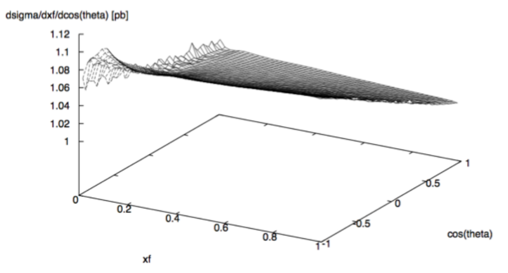
respectively, compared to the current limit of . Model-independently, would be sensitive to new physics with (1) couplings up to scales of about 70 TeV. Also, the precision in the parameters entering the -vertex (one of which currently showing a 2.7 deviation) would improve by an order of magnitude.
Acknowledgements
I gratefully acknowledge support by Alain Blondel and the University of Geneva.
13 Composite Higgs Models at Colliders
Stefania De Curtis
A future collider will be capable to show the imprint of composite Higgs scenarios encompassing partial compositeness. Besides the detailed study of the Higgs properties, such a machine will have a rich top-quark physics program mainly in two domains: top property accurate determination at the production threshold, search for New Physics (NP) with top quarks above the threshold. In both domains, a composite Higgs scenario can show up. Here we discuss such possibility using a particular realisation, namely the 4-Dimensional Composite Higgs Model (4DCHM) [99]. It describes the intriguing possibility that the Higgs particle may be a composite state arising from some strongly interacting dynamics at a high scale. This will solve the hierarchy problem owing to compositeness form factors taming the divergent growth of the Higgs mass upon quantum effects. Furthermore, the now measured light mass could be consistent with the fact that the composite Higgs arises as a pseudo Nambu-Goldstone Boson (pNGB) from a particular coset of a global symmetry breaking. Models with a pNGB Higgs generally predict modifications of its couplings to both bosons and fermions of the SM, hence the measurement of these quantities represents a powerful way to test its possible non-fundamental nature. Furthermore, the presence of additional particles in the spectrum of such composite Higgs models (CHMs) leads to both mixing effects with the SM states as well as new Feynman diagram topologies both of which would represent a further source of deviations from the SM expectations.
In the near future, the LHC will be able to test Beyond-Standard-Model (BSM) scenarios more extensively, probing the existence of new particles predicted by extensions of the SM to an unprecedented level. Nevertheless the expected bounds, though severe, could not be conclusive to completely exclude natural scenarios for the Fermi scale. As an example, new gauge bosons predicted by CHMs with mass larger than 2 TeV could escape the detection of the LHC [100]. Furthermore, concerning the Higgs properties, the LHC will not be able to measure the Higgs couplings to better than few % leaving room to scenarios, like CHMs, which predict deviations within the foreseen experimental accuracy for natural choices of the compositeness scale , (namely in the TeV range) and of the strong coupling constant . For these reasons we will face here the case in which LHC will not discover a (or not be able to clearly asses its properties) and also will not discover any extra fermion (or it will discover it with a mass around 800 GeV, which is roughly the present bound, but without any other hint about the theory to which it belongs). In this situation, an collider could have a great power for enlightening indirect effects of BSM physics.
The main Higgs production channels within the 4DCHM were considered in [101] for three possible energy stages and different luminosity options of the proposed machines, and the results were confronted to the expected experimental accuracies in the various Higgs decay channels. Moreover the potentialities of such colliders in discovering the imprint of partial compositeness in the top-quark sector through an accurate determination of the top properties at the production threshold were analized in [102]. In Fig. 10 we compare the deviations for the and couplings and in Fig. 11(left panel) for the and couplings in the 4DCHM with the relative precision expected at HL-LHC, ILC, FCC-ee [102, 82, 6, 103]
From the Higgs coupling measurements, it is clear that the FCC-ee will be able to discover CHMs with a very large significance, also for values of larger than 1 TeV for which the LHC measurements will not be sufficient to detect deviations from the SM. This is true a fortiori for the top electroweak coupling measurements. In fact an collider can separately extract the left- and right-handed electroweak couplings of the top. This is particularly relevant for models with partially composite top, like the 4DCHM where the coupling modification comes not only from the mixing of the with the s but also from the mixing of the top (antitop) with the extra-fermions (antifermions), as expected by the partial compositeness mechanism. For the "natural" scan described in the caption of Fig. 10, the typical deviations lie within the region uncovered by the HL-LHC but are well inside the reach of the polarized ILC-500 and the FCC-ee where the lack of initial polarization is compensated by the presence of a substantial final state polarization and by a larger integrated luminosity [82, 6, 103].
But this is not the end of the story, in fact in CHMs the modifications in the and processes arise not only via the modification of the coupling for the former and of the coupling for the latter, but also from the exchange of new particles, namely the -channel exchange of ts, which can be sizeable also for large masses due to the interference with the SM states. This effect can be crucial at high c.o.m energies of the collider but also important at moderate [82]. In particular it is impressive how the FCC-ee with GeV and 2.6 ab-1 (corresponding to 3 years of operation) could discover the imprint of extra particles through their effective contribution to the EW top coupling deviations. This result emerges from the optimal-observable analysis of the lepton angular and energy distributions from top-quark pair production with semi-leptonic decays [81, 6, 102]. The , vertices can be expressed in the usual way in terms of 8 form factors:
| (15) |
and the differential cross-section for the process: can be expanded around their SM values:
| (16) |
Here gives the SM contribution, and are the lepton reduced energy and the polar angle. By considering only the 6 CP-conserving form factors (), the elements of the covariance matrix (the statistical uncertainties) are derived from a likelihood fit to the lepton angular/energy distributions and the total event rate [6]. The result for the top pair left- and right-handed couplings to the is represented by the continous green ellipses in Fig. 10.
In order to compare these uncertainties with the deviations expected in CHMs (deviations in the form factors due not only to coupling modifications but also to s exchanges) we have considered one representative benchmark point of the 4DCHM (point-A) corresponding to TeV, =1.5, =1.4 TeV ( is the scale of the extra-fermion mass). This scenario describes two nearly degenerate s, with mass 2.1 and 2.2 TeV respectively, which are active in the top pair production. The deviations in the and couplings are and as shown by the yellow point in Fig. 11(right) , while .
As an exercise, we have evaluated the double differential cross section of Eq. 16 within the 4DCHM without including the exchanges and extracted the deviations in the and photon left and right couplings to the top pair by performing a 4 parameter fit (i.e. fixing the other two CP conserving form factors, , to their SM value). The result is shown in Fig. 12. The ellipses correspond to 1,2,3 . As expected the deviations in the photon couplings are fully compatible with zero. Also, the central values of the coupling deviations reproduce very well the deviations corresponding to the point-A ( to be compared with and to be compared with where we have included the marginalized uncertainties). The fit is very good in reproducing the theoretical deviations for the couplings, but, as said, this is an exercise. In fact the s were taken off.
The double differential cross section within the full 4DCHM normalized to the SM one is shown in the bottom-left panel of Fig. 13, while the deviations in the and photon left and right "effective" couplings to the top pair extracted by performing a 4 parameter fit, are shown in Fig. 14. We called them "effective" couplings because they include the effects of the interference of the s with the SM gauge bosons. This is clearly evident by looking at the deviations of the photon couplings, which are completely due to these interference effects.
These results, derived here for a single benchmark point, are very promising and show the importance of the interference between the SM and the s already at =365 GeV. A more detailed analysis is worth to be done [104] to extract the dependence of the effective EW top couplings from the properties (mass and couplings, the width is not important at such moderate energies) in order to clearly relate them to these new spin-1 particles which are naturally present in CHMs. The optimal-observable statistical analysis at FCC-ee offers a unique possibility to disentangle the effects of top coupling modifications (always taken into account in NP searches) from interference effects (often neglected).




14 Constraints on top FCNC’s from (hadronic) single top production in collisions
S. Biswas,F. Margaroli, B. Mele
Single top production in colliders is a sensitive probe of anomalous Flavor Changing Neutral Currents (FCNC) in the top sector. In particular, the production (with ), mediated by an -channel photon and vector boson has undetectably small rates in the standard model (SM), but might become visible for - and -coupling strenghts allowed by various beyond-the-SM theoretical frameworks, and not excluded by present experiments [16]. Single top production has two advantages with respect to top pair production above the threshold, where FCNC’s can be probed in top decays. On the one hand, it can be studied at lower (more easily accessible) c.m. energies, such as GeV which optimizes Higgs-boson studies. On the other hand, since the FCNC and couplings in are active in production, one can enhance the sensitivity to the magnetic-dipole-moment part () of the FCNC Lagrangian by increasing the collision energy . This feature can even make the single top production more sensitive to FCNC couplings than top-pair production at energies above the threshold [16].
Here we report the results of a recent analysis of the sensitivity reach on FCNC and couplings at GreV, with the top quark decaying hadronically. Indeed, the exceptionally clean environment and the great particle-identification capabilities expected at future detectors will allow to fully exploit events with hadronic top decays, with a control and separation of background never experienced before in top quark studies. The relevant FCNC couplings (assuming no related parity violation) are defined by the lagrangian : . The couplings can be straightforwardly related to the corresponding decay branching ratios , , .
The signal, and main background (other 4-jets background like have been checked to be negligible) have been generated via MadGraph5_aMC@NLO (with FeynRules modeling the FCNC interactions), and interfaced with PYTHIA for showering and hadronization. Jets have been defined by PYTHIA iterative cone algorithm with cone size , and jet energy resolution has been parametrized as . The -tagging efficiency and corresponding fake jet rejection for and light-quark jets are crucial, since the background does not contain -quark initiated jets. We have worked with two hypothesis : a) true -jet tagging efficiency of , and corresponding -(light)-jet rejection factor of 250 (1000); b) with -(light)-jet rejection factor 10 (100) [106]. An optimized choice of fake jet rejection factors indeed proved to be more useful than a large -tagging efficiency. Basic cuts applied on jets are GeV, , and . Through an MVA study we have then identified a further set of cuts, improving the background rejection: a) a di-jet system inside the mass window 65 GeV 90 GeV (compatibility with ); b) rejection of events if invariant mass of the remaining di-jet system peaks around a second within a mass window 65 GeV 85 GeV; c) a jet tagged as a -jet is then combined with the reconstructed , and required to produce a top system satisfying 150 GeV 175 GeV; d) finally, the jet which is neither a -jet nor a jet coming from a -decay is required to have 65 GeV.
The final bounds on FCNC couplings and corresponding Br’s are reported for different integrated luminosities L in Table 1. With L=100 fb-1, we find that the hadronic top channel has about twice the sensitivity to BR’s as the semileptonic top channel [107].
| ( | BR | BR | ||
| L=0.5 ab-1 | 1.8 | 1.4 | 3.3 | 4.7 |
| L=10 ab-1 | 8.6 | 3.2 | 1.6 | 1.1 |
| ( | BR | BR | ||
| L=0.5 ab-1 | 2.8 | 3.8 | 5.1 | 1.2 |
| L=10 ab-1 | 1.3 | 8.2 | 2.4 | 2.8 |
| ( | BR | BR | ||
| L=0.5 ab-1 | 2.2 | 1.9 | 4.1 | 6.1 |
| L=10 ab-1 | 1.1 | 4.1 | 1.9 | 1.4 |
15 EFT approach to top-quark physics at FCC-ee
Cen Zhang
At high-energy colliders, precision measurements play an important role in the search for physics beyond the standard model (SM). In this respect, the top quark is often considered as a window to new physics, thanks to its large mass. Results from the LHC measurements already provided valuable information on possible deviations [97]. Future lepton colliders such as FCC-ee have been proposed to complement the search program at the LHC, with much higher sensitivities expected.
A general theoretical framework where the experimental information on possible deviations from the SM can be consistently and systematically interpreted is provided by the effective field theory (EFT) approach [108, 109, 110]. The EFT Lagrangian corresponds to that of the SM augmented by higher-dimensional operators that respect the symmetries of the SM. It provides a powerful approach to identify observables where deviations could be expected in the top sector, and allows for a global interpretation of all available measurements. In the following, we briefly discuss several features of the approach, and the corresponding implications for top physics at future lepton colliders.
First of all, EFT is a global approach where all possible deviations from the SM are allowed in the framework, provided that the new physics scale is heavier than the scale of the experiment. Hence all precision measurements can be taken into account in this one approach, allowing for a global analysis of the world’s data. Such an analysis for the top quark has been carried out already for direct measurements at the Tevatron and the LHC Run-I [111, 112]. Other indirect measurements can be analyzed and combined in the same way, for example those from precision electroweak data [113, 114] and from flavor data [115]. As we move on to future colliders, it is important to continue this program within the same framework, to fully exploit all the knowledge at hand.
Second, unlike the “anomalous coupling” parametrization (see, e.g. Ref. [116]) that focuses on specific vertices, the EFT description is more complete, allowing for analyzing certain classes of interactions that are not captured in the “anomalous coupling” approach, and are often overlooked. For example, the four-fermion interactions involving two leptons and two quarks, such as
are well motivated as they can be easily generated by integrating out a tree-level heavy mediator in certain new physics scenarios, but are not well constrained at the LHC. There are measurements on production which could give some information [117], but the uncertainties there are quite large, and the process itself is not very sensitive to the operators. On the other hand, at future lepton colliders the process is much cleaner, and the sensitivity to the operators are at least two orders of magnitude better. Another interesting scenario is the flavor-changing neutral (FCN) interactions coupled to heavy particles. These interactions are described by similar operators, such as
where is the flavor index. The FCN four-fermion operators have constraints from at LEP2 and at the LHC [118]. One might think that the LHC gives much tighter bounds on FCN couplings than LEP2; it turns out that this is true for two-fermion FCN couplings (such as a vertex), but is not the case for the four-fermion ones, mainly because the top-quark three-body decays are suppressed. This is reflected in Figure 1, where current bounds on the two types of FCN operators are compared. It follows that future lepton collider will provide much more accurate information on FCN interactions coupled to heavy mediators, and an EFT approach should be used to capture these interactions and incorporate them in a global study.
Finally, EFT allows for higher-order corrections to be consistently added, and therefore predictions can be systematically improved. This is important not only for the LHC where QCD corrections are always large, but also for lepton colliders as the expected precision level is much higher. Recently a set of effective operators that parametrize the chromo-dipole and the electroweak couplings of the top quark have been implemented in the MadGraph5_aMC@NLO [119] framework at next-to-leading order (NLO) in QCD [120, 121]. As a result, starting from an EFT with these operators, one can make NLO predictions for various top-quark processes, for cross sections as well as distributions, in a fully automatic way. Furthermore, NLO results matched to the parton shower simulation are available, so event generation can be and should be directly employed in future experimental analyses. These works provide a solid basis for the interpretation of measurements both at the LHC and at possible future colliders. As an example, in Table 1 we show the contribution of various operators in process at a center-of-mass energy of 500 GeV.
| 500GeV | SM | ||||||
|---|---|---|---|---|---|---|---|
| 566 | 0 | 15.3 | -15.3 | -1.3 | 272 | 191 | |
| 647 | -6.22 | 18.0 | -18.0 | -1.0 | 307 | 216 | |
| K-factor | 1.14 | N/A | 1.17 | 1.17 | 0.78 | 1.13 | 1.13 |

16 W mass and width determination using the WW threshold cross section
Paolo Azzurri
The W mass is a fundamental parameter of the standard model (SM) of particle physics, currently measured with a precision of 15 MeV [122]. In the context of precision electroweak precision tests the direct measurement of the W mass is currently limiting the sensitivity to possible effects of new physics [19].
A precise direct determination of the W mass can be achieved by observing the rapid rise of the W-pair production cross section near its kinematic threshold. The advantages of this method are that it only involves counting events, it is clean and uses all decay channels.
In 1996 the LEP2 collider delivered collisions at a single energy point near 161 GeV, with a total integrated luminosity of about 10 pb-1 at each of the four interaction points. The data was used to measure the W-pair cross section () at 161 GeV, and extract the W mass with a precision of 200 MeV [123, 124, 125, 126].
In the SM the W width is well constrained by the W mass, and the Fermi constant, with a QCD correction coming from hadronic decays; the W width is currently measured to a precision of 42 MeV [122]. The first calculations of the W boson width effects in reactions have been performed in Ref. [127], and revealed the substantial effects of the width on the full cross section lineshape, in particular at energies below the nominal threshold.
In this study the possibility of extracting both the W mass and width from the determination of at a minimum of two energy points near the kinematic threshold is explored.
The YFSWW3 version 1.18 [128] program has been used to calculate as a function of the energy (), W mass () and width (). Figure 16 shows the W-pair cross section as a function of the collision energy with W mass and width values set at the PDG [122] average measured central values GeV and GeV, and with large 1 GeV variation bands of the mass and width central values.

It can be noted that while a variation of the W mass roughly corresponds to a shift of the cross section lineshape along the energy axis, a variation of the W width has the effect of changing the slope of cross section lineshape rise. It can also be noted that the W width dependence shows a crossing point at GeV, where the cross section is insensitive to the W width.
16.1 W mass measurement at a single energy point
Detailed studies have illustrated the possibility of obtaining a precision W mass determination by further exploiting the threshold W pair production measurement at future colliders [129, 130].
Taking data at a single energy point the statistical sensitivity to the W mass with a simple event counting is given by
| (17) |
where is the data integrated luminosity, the event selection efficiency and the selection purity. The purity can be also expressed as
where is the total selected background cross section.
A systematic uncertainty on the background cross section will propagate to the W mass uncertainty as
| (18) |
Other systematic uncertainties as on the acceptance () and luminosity () will propagate as
| (19) |
while theoretical uncertainties on the cross section () propagate directly as
| (20) |
Finally the uncertainty on the center of mass energy will propagate to the W mass uncertainty as
| (21) |
that can be shown to be limited as , and in fact for near the threshold it is , so it is the beam energy uncertainty that propagates directly to the W mass uncertainty.
In the case of ab-1 accumulated by the FCCee data taking in one year, and assuming the LEP event selection quality [123] with fb and , a statistical precision of MeV is achievable if the systematic uncertainties will not be limiting the precision, i.e. if the following conditions are achieved:
| (22) | |||
| (23) | |||
| (24) | |||
| (25) |
corresponding to precision levels of on the background, on acceptance and luminosity, on the theoretical cross section, and on the beam energy.
16.2 W mass and width measurements at two energy points
Figures 17 and 18 show the differential functions relevant to the statistical and systematical uncertainties discussed above. For the statistical terms the efficiency and purities are evaluated assuming an event selection quality with fb and .


The minima of the mass differential curves plotted in Fig. 17 indicate the optimal points to take data for a W mass measurement, in particular minimum statistical uncertainty is achieved with GeV GeV. The minima of the width differential curves, on Fig. 18, indicate maximum sensitivity to the W width, while all curves diverge at the W width insensitive point GeV, where .
If two cross section measurements are performed at two energy points , both the W mass and width can be extracted with a fit to the cross section lineshape. The uncertainty propagation would then follow
| (26) | |||
| (27) |
The resulting uncertainty on the W mass and width would be
| (28) |
| (29) |
If the uncertainties on the cross section measurements are uncorrelated, e.g. only statistical, the linear correlation between the derived mass and width uncertainties is
| (30) |
16.3 Optimal data taking configurations
When conceiving data taking at two different energy points near the W-pair threshold in order to extract both and , it is useful to figure out which energy points values and , would be optimally suited to obtain the best measurements, also as a function of the data luminosity fraction delivered at the lower energy point. For this a full 3-dimensional scan of possible and values, with 100 MeV steps, and of values, with 0.05 steps, has been performed, and the data taking configurations that minimize arbitrary combination of the expected statistical uncertainties on the mass and the width are found.
In order to minimize the simple sum of the statistical uncertainties , the optimal data taking configuration would be with
| (31) |
With this configuration, and assuming a total luminosity of ab-1, the projected statistical uncertainties would be
| (32) |
With this same data taking configuration,the statistical uncertainty obtained when measuring only the W mass would yield MeV, just slightly better with respect to the two-parameter fit. On the other hand the MeV precision obtained in this way must be compared with the MeV statistical precision obtainable when taking all data at the most optimal single energy point GeV.
When varying the target to optimize towards, the obtained optimal energy points don’t change much, with the upper energy always at the -independent GeV point, and the optimal lower point at units below the nominal threshold, , according to if the desired precision is more or less focused on the W mass or the W width measurement. In a similar way the optimal data fraction to be taken at the lower off-shell energy point varies according to the chosen precision targets, with larger fractions more to the benefit of the W width precision. When a small fraction of data (e.g. 0.05) is taken off-shell a statistical precision MeV is recovered both in the single- () and the two-parameter () fits.
17 Summary
The goal of the mini-workshop ”Physics behind Precision” was to provide inspiration for new work on precision physics for FCC-ee in the realm of top quark and electroweak precision physics. The covered topics included Electroweak physics at the Z boson peak, the physics of the threshold at colliders and W boson physics at the threshold. The mini-workshop also allowed the possibility of discussing the details of recent event generator developments. The studies confirm that for most scenarios the FCC-ee will reduce experimental errors by factors of 10 or more compared to LEP/SLC. This indicates the need for developments in theory to keep the theory uncertainties of similar order.
The mini-workshop succeded in attracting the main proponents from different communities in theory, experiments and tools. The productive discussion during the workshop has resulted in these (online) proceedings. In the future the community aims to further incorporate these and new results on top quark and electroweak precision physics into the FCC-ee Conceptual Design Report under preparation.
References
- [1] Physics Beyond Precision, https://indico.cern.ch/event/469561/, note = CERN indico page, contains many of the talk contributions, year = 2016,.
- [2] S. Schael et al. Precision electroweak measurements on the resonance. Phys. Rept., 427:257–454, 2006.
- [3] S. Schael et al. Electroweak Measurements in Electron-Positron Collisions at W-Boson-Pair Energies at LEP. Phys. Rept., 532:119–244, 2013.
- [4] Paul Langacker. The standard model and beyond. High Energy Physics, Cosmology and Gravitation. Taylor and Francis, Boca Raton, FL, 2010.
- [5] M. Bicer, H. Duran Yildiz, I. Yildiz, G. Coignet, M. Delmastro, et al. First Look at the Physics Case of TLEP. 2013.
- [6] Patrick Janot. Top-quark electroweak couplings at the FCC-ee. JHEP, 04:182, 2015.
- [7] Keisuke Fujii et al. Physics Case for the International Linear Collider. 2015.
- [8] Howard Baer, Tim Barklow, Keisuke Fujii, Gao Yuanning, Andre Hoang, et al. The International Linear Collider Technical Design Report - Volume 2: Physics. 2013.
- [9] Halina Abramowicz et al. The International Linear Collider Technical Design Report - Volume 4: Detectors. 2013.
- [10] T. Barklow, J. Brau, K. Fujii, J. Gao, J. List, N. Walker, and K. Yokoya. ILC Operating Scenarios. 2015.
- [11] Lucie Linssen, Akiya Miyamoto, Marcel Stanitzki, and Harry Weerts. Physics and Detectors at CLIC: CLIC Conceptual Design Report. 2012.
- [12] M Aicheler, P Burrows, M Draper, T Garvey, P Lebrun, K Peach, N Phinney, Schmickler H, D Schulte, and N Toge. A Multi-TeV Linear Collider Based on CLIC Technology. 2012.
- [13] M J Boland et al. Updated baseline for a staged Compact Linear Collider. 2016.
- [14] CEPC-SPPC Study Group. CEPC-SPPC Preliminary Conceptual Design Report. 1. Physics and Detector, IHEP-CEPC-DR-2015-01 (2015). 2015.
- [15] Yuri Alexahin et al. Muon Collider Higgs Factory for Snowmass 2013. In Community Summer Study 2013: Snowmass on the Mississippi (CSS2013) Minneapolis, MN, USA, July 29-August 6, 2013, 2013.
- [16] K. Agashe et al. Working Group Report: Top Quark. In Community Summer Study 2013: Snowmass on the Mississippi (CSS2013) Minneapolis, MN, USA, July 29-August 6, 2013, 2013.
- [17] M. Vos et al. Top physics at high-energy lepton colliders. 2016.
- [18] S. Gusken, Johann H. Kuhn, and P. M. Zerwas. Threshold Behavior of Top Production in Annihilation. Phys. Lett., B155:185, 1985.
- [19] M. Baak et al. The global electroweak fit at NNLO and prospects for the LHC and ILC. 2014.
- [20] Giuseppe Degrassi, Stefano Di Vita, Elias-Miro Joan, Jose R. Espinosa, Gian F. Giudice, Gino Isidori, and Alessandro Strumia. Higgs mass and vacuum stability in the Standard Model at NNLO. JHEP, 08:098, 2012.
- [21] Martin Beneke, Yuichiro Kiyo, Peter Marquard, Alexander Penin, Jan Piclum, and Steinhauser Matthias. Next-to-Next-to-Next-to-Leading Order QCD Prediction for the Top Antitop -Wave Pair Production Cross Section Near Threshold in Annihilation. Phys. Rev. Lett., 115(19):192001, 2015.
- [22] André H. Hoang and Maximilian Stahlhofen. The Top-Antitop Threshold at the ILC: NNLL QCD Uncertainties. JHEP, 05:121, 2014.
- [23] Peter Marquard, Alexander V. Smirnov, Smirnov Vladimir A., and Matthias Steinhauser. Quark Mass Relations to Four-Loop Order in Perturbative QCD. Phys. Rev. Lett., 114(14):142002, 2015.
- [24] Katja Seidel, Frank Simon, Michal Tesar, and Stephane Poss. Top quark mass measurements at and above threshold at CLIC. Eur. Phys. J., C73(8):2530, 2013.
- [25] Tomohiro Horiguchi, Akimasa Ishikawa, Suehara Taikan, Keisuke Fujii, Yukinari Sumino, Kiyo Yuichiro, and Hitoshi Yamamoto. Study of top quark pair production near threshold at the ILC. 2013.
- [26] Manel Martinez and Ramon Miquel. Multiparameter fits to the t anti-t threshold observables at a future e+ e- linear collider. Eur. Phys. J., C27:49–55, 2003.
- [27] Frank Simon. A First Look at the Impact of NNNLO Theory Uncertainties on Top Mass Measurements at the ILC. In International Workshop on Future Linear Colliders (LCWS15) Whistler, B.C., Canada, November 2-6, 2015, 2016.
- [28] Aurelio Juste, Sonny Mantry, Alexander Mitov, Alexander Penin, Peter Skands, Erich Varnes, Marcel Vos, and Stephen Wimpenny. Determination of the top quark mass circa 2013: methods subtleties, perspectives. Eur. Phys. J., C74(10):3119, 2014.
- [29] Projected improvement of the accuracy of top-quark mass measurements at the upgraded LHC. CMS-PAS-FTR-13-017.
- [30] Mathias Butenschoen, Bahman Dehnadi, Andre H. Hoang, Vicent Mateu, Moritz Preisser, and Stewart Iain W. Top Quark Mass Calibration for Monte Carlo Event Generators. 2016.
- [31] Andre H. Hoang and I W Stewart. Top-mass measurements from jets and the Tevatron top mass. Nouvo Cimento, B123:1092–1100, 2008.
- [32] S. Moch et al. High precision fundamental constants at the TeV scale. 2014.
- [33] Andre H. Hoang. The Top Mass: Interpretation and Theoretical Uncertainties. 2014.
- [34] Gennaro Corcella. Interpretation of the top-quark mass measurements: a theory overview. PoS, TOP2015:037, 2016.
- [35] M. L. Mangano et al. Physics at a 100 TeV pp collider: Standard Model processes. 2016.
- [36] M. S. Amjad, M. Boronat, T. Frisson, Garcia I., R. Poschl, E. Ros, F. Richard, Rouene J., P. Ruiz Femenia, and M. Vos. A precise determination of top quark electro-weak couplings at the ILC operating at GeV. 2013.
- [37] M. S. Amjad et al. A precise characterisation of the top quark electro-weak vertices at the ILC. Eur. Phys. J., C75(10):512, 2015.
- [38] P. H. Khiem, E. Kou, Y. Kurihara, and Diberder F. Le. Probing New Physics using top quark polarization in the process at future Linear Colliders. 2015.
- [39] Raoul R¨oentsch and Markus Schulze. Constraining the top- coupling through production at the LHC. Nucl. Part. Phys. Proc., 273-275:2311–2316, 2016.
- [40] J. A. Aguilar-Saavedra et al. TESLA: The Superconducting electron positron linear collider with an integrated x-ray laser laboratory. Technical design report. Part 3. Physics at an e+ e- linear collider. 2001.
- [41] H. Abramowicz et al. Higgs Physics at the CLIC Electron-Positron Linear Collider. 2016.
- [42] Tony Price, Philipp Roloff, Jan Strube, and Tomohiko Tanabe. Full simulation study of the top Yukawa coupling at the ILC at 1 TeV. Eur. Phys. J., C75(7):309, 2015.
- [43] Sally Dawson et al. Working Group Report: Higgs Boson. In Community Summer Study 2013: Snowmass on the Mississippi (CSS2013) Minneapolis, MN, USA, July 29-August 6, 2013, 2013.
- [44] Aleksander Filip Żarnecki. Top physics at CLIC and ILC. In 38th International Conference on High Energy Physics (ICHEP 2016) Chicago, USA, August 3-10, 2016, 2016.
- [45] Raoul Röentsch and Markus Schulze. Constraining the top- coupling through production at the LHC. Nucl. Part. Phys. Proc., 273-275:2311–2316, 2016.
- [46] Raoul Röentsch and Markus Schulze. Probing top-Z dipole moments at the LHC and ILC. JHEP, 08:044, 2015.
- [47] U. Baur, A. Juste, L. H. Orr, and D. Rainwater. Probing electroweak top quark couplings at hadron colliders. Phys. Rev., D71:054013, 2005.
- [48] First combination of Tevatron and LHC measurements of the top-quark mass. 2014.
- [49] Vardan Khachatryan et al. Measurement of the top quark mass using proton-proton data at = 7 and 8 TeV. Phys. Rev., D93(7):072004, 2016.
- [50] M. Beneke and Vladimir M. Braun. Heavy quark effective theory beyond perturbation theory: Renormalons, the pole mass and the residual mass term. Nucl. Phys., B426:301–343, 1994.
- [51] Paolo Nason. Theory Summary. PoS, TOP2015:056, 2016.
- [52] Andre H. Hoang and Iain W. Stewart. Top Mass Measurements from Jets and the Tevatron Top-Quark Mass. Nucl. Phys. Proc. Suppl., 185:220–226, 2008.
- [53] Gennaro Corcella. Hadronization systematics and top mass reconstruction. EPJ Web Conf., 80:00019, 2014.
- [54] CMS Collaboration. Measurement of the ttbar production cross section in the emu channel in pp collisions at 7 and 8 TeV. 2015.
- [55] Georges Aad et al. Measurement of the production cross-section using events with b-tagged jets in pp collisions at = 7 and 8 with the ATLAS detector. Eur. Phys. J., C74(10):3109, 2014. [Addendum: Eur. Phys. J.C76,no.11,642(2016)].
- [56] Georges Aad et al. Determination of the top-quark pole mass using + 1-jet events collected with the ATLAS experiment in 7 TeV pp collisions. JHEP, 10:121, 2015.
- [57] Michał Czakon, Paul Fiedler, and Alexander Mitov. Total Top-Quark Pair-Production Cross Section at Hadron Colliders Through . Phys. Rev. Lett., 110:252004, 2013.
- [58] Simone Alioli, Patricia Fernandez, Juan Fuster, Adrian Irles, Sven-Olaf Moch, Peter Uwer, and Marcel Vos. A new observable to measure the top-quark mass at hadron colliders. Eur. Phys. J., C73:2438, 2013.
- [59] Serguei Chatrchyan et al. Measurement of masses in the system by kinematic endpoints in pp collisions at = 7 TeV. Eur. Phys. J., C73:2494, 2013.
- [60] Kaustubh Agashe, Roberto Franceschini, Kim Doojin, and Markus Schulze. Top quark mass determination from the energy peaks of b-jets and B-hadrons at NLO QCD. Eur. Phys. J., C76(11):636, 2016.
- [61] CMS Collaboration. Measurement of the top-quark mass from the b jet energy spectrum. 2015.
- [62] CMS Collaboration. Determination of the top-quark mass from the m(lb) distribution in dileptonic ttbar events at sqrt(s) = 8 TeV. 2014.
- [63] R. Chierici and A. Dierlamm. Determination of the top mass with exclusive events t —> W b —> l nu J/psi X. 2006.
- [64] A. H. Hoang and T. Teubner. Top quark pair production close to threshold: Top mass width and momentum distribution. Phys. Rev., D60:114027, 1999.
- [65] M. Beneke. A Quark mass definition adequate for threshold problems. Phys. Lett., B434:115–125, 1998.
- [66] K. Melnikov T. Nagano A. Ota A. A. Penin A. A. Pivovarov A. H. Hoang, M. Beneke and A. Signer et al. Eur. Phys. J., C2(1), 2000. hep-ph/001286.
- [67] M. Beneke, Y. Kiyo, and K. Schuller. Third-order correction to top-quark pair production near threshold I. Effective theory set-up and matching coefficients. 2013.
- [68] V. A. Smirnov A. V. Smirnov and M. Steinhauser. Phys. Lett. B, 668:293, 2008.
- [69] V. A. Smirnov A. V. Smirnov and M. Steinhauser. Phys.Rev.Lett., 104:112002, 2010.
- [70] Y.Kiyo C.Anzai and Y. Sumino. Phys.Rev.Lett., 104:112003, 2010.
- [71] D. Seidel P. Marquard, J. H. Piclum and M. Steinhauser. Nucl.Phys.B, 758:144, 2006.
- [72] D. Seidel P. Marquard, J. H. Piclum and M. Steinhauser. Phys.Lett.B, page 269, 2009.
- [73] D. Seidel P. Marquard, J. H. Piclum and M. Steinhauser. Phys.Lett., D 89(3):034027.
- [74] M. Beneke and Y.Kiyo. Phys.Lett.B, 668:143, 2008.
- [75] Y.Kiyo M. Beneke and K.Schuller. Nucl.Phys.B, 714:67, 2005.
- [76] Y.Kiyo M. Beneke and K.Schuller. Third-order correction to top-quark pair production near theshold II. Potential contributions. to be published.
- [77] Martin Beneke, Andreas Maier, Jan Piclum, and Thomas Rauh. Nucl. Phys.B, 899:180–193, 2015.
- [78] Peter Marquard, Alexander V. Smirnov, Vladimir A. Smirnov, and Matthias Steinhauser. Four-loop relation between the and on-shell quark mass. In Proceedings, 12th International Symposium on Radiative Corrections (Radcor 2015) and LoopFest XIV (Radiative Corrections for the LHC and Future Colliders), 2016.
- [79] Wolfgang Kilian, Thorsten Ohl, and Jurgen Reuter. WHIZARD: Simulating Multi-Particle Processes at LHC and ILC. Eur. Phys. J., C71:1742, 2011.
- [80] O. Wendt, F. Gaede, and T. Kramer. Event Reconstruction with MarlinReco at the ILC. Pramana, 69:1109–1114, 2007.
- [81] Bohdan Grzadkowski and Zenro Hioki. Optimal observable analysis of the angular and energy distributions for top quark decay products at polarized linear colliders. Nucl. Phys., B585:3–27, 2000. [Erratum: Nucl. Phys.B894,585(2015)].
- [82] Daniele Barducci, Stefania De Curtis, Stefano Moretti, and Giovanni Marco Pruna. Top pair production at a future machine in a composite Higgs scenario. JHEP, 08:127, 2015.
- [83] Torbjörn Sjöstrand, Stefan Ask, Christiansen Jesper R., Richard Corke, Nishita Desai, Ilten Philip, Stephen Mrenna, Stefan Prestel, Christine O. Rasmussen, and Peter Z. Skands. An Introduction to PYTHIA 8.2. Comput. Phys. Commun., 191:159–177, 2015.
- [84] F. Cornet, P. Jankowski, M. Krawczyk, and Lorca A. A New five flavor LO analysis and parametrization of parton distributions in the real photon. Phys. Rev., D68:014010, 2003.
- [85] Torbjörn. Sjöstrand and Peter Z. Skands. Transverse-momentum-ordered showers and interleaved multiple interactions. Eur. Phys. J., C39:129–154, 2005.
- [86] Torbjörn. Sjöstrand and Peter Z. Skands. Multiple interactions and the structure of beam remnants. JHEP, 03:053, 2004.
- [87] T. Ohl M. Moretti and J. Reuter. hep-ph/0102195.
- [88] T. Ohl. Comput.Phys.Commun., 120:13, 1999.
- [89] S. Schmidt W. Kilian, J. Reuter and D. Wiesler. JHEP, 1204:013, 2012.
- [90] A. L. Kataev S. Eidelman, F. Jegerlehner and O. Veretin. Phys. Lett. B, 454(369):0370–2693, 1999.
- [91] F. Jegerlehner. Nucl. Phys. Proc. Suppl., 162, 2006.
- [92] L. Trentadue G. Venanzoni C. M. Carloni Calame, M. Passera. Phys. Lett. B, 746, 2015.
- [93] Patrick Janot. Direct measurement of at the FCC-ee. JHEP, 02:053, 2016.
- [94] S. Jadach, B. F. L. Ward, and Z. Was. Coherent exclusive exponentiation for precision Monte Carlo calculations. Physical Review D, 63(11), may 2001.
- [95] M. Greco, G. Pancheri-Srivastava, and Y. Srivastava. Radiative effects for resonances with applications to colliding beam processes. Physics Letters B, 56(4):367–372, may 1975.
- [96] M. Greco, F. Palumbo, G. Pancheri-Srivastava, and Y. Srivastava. Coherent state approach to the infra-red behaviour of non-abelian gauge theories. Physics Letters B, 77(3):282–286, aug 1978.
- [97] K. A. Olive et al. Review of Particle Physics. Chin. Phys., C38:090001, 2014.
- [98] X. Lu B. Henning and H. Murayama. JHEP, 1601:023, 2016.
- [99] Stefania De Curtis, Michele Redi, and Andrea Tesi. The 4D Composite Higgs. JHEP, 04:042, 2012.
- [100] Daniele Barducci, Alexander Belyaev, De Curtis Stefania, Stefano Moretti, and Giovanni Marco Pruna. Exploring Drell-Yan signals from the 4D Composite Higgs Model at the LHC. JHEP, 04:152, 2013.
- [101] Daniele Barducci, Stefania De Curtis, Moretti Stefano, and Giovanni Marco Pruna. Future Electron-Positron Colliders and the 4-Dimensional Composite Higgs Model. JHEP, 02:005, 2014.
- [102] Patrick Janot. Precision measurements of the top quark couplings at the FCC. PoS, EPS-HEP2015:333, 2015.
- [103] A. Andreazza et al. What Next: White Paper of the INFN-CSN1. Frascati Phys. Ser., 60:1–302, 2015.
- [104] P. Janot De Curtis and S. Moretti. in preparation.
- [105] Francois Richard. Present and future constraints on top EW couplings. 2014.
- [106] N. Alipour Tehrani. Optimisation studies for the clic vertex-detector geometry. Journal of Instrumentation, 10(07):C07001, 2015.
- [107] M.K.Yanehsari Khanpour, S.Khatibi and M.M.Najafabadi. Single top quark production as a probe of anomalous and couplings at the FCC-ee. arXiv:1408.2090.
- [108] Steven Weinberg. Phenomenological Lagrangians. Physica, A96:327, 1979.
- [109] W. Buchmuller and D. Wyler. Effective Lagrangian Analysis of New Interactions and Flavor Conservation. Nucl. Phys., B268:621–653, 1986.
- [110] Chung Ngoc Leung, S. T. Love, and S. Rao. Low-Energy Manifestations of a New Interaction Scale: Operator Analysis. Z. Phys., C31:433, 1986.
- [111] Andy Buckley, Christoph Englert, James Ferrando, David J. Miller, Liam Moore, Michael Russell, and Chris D. White. Constraining top quark effective theory in the LHC Run II era. 2015.
- [112] Andy Buckley, Christoph Englert, James Ferrando, David J. Miller, Liam Moore, Michael Russell, and Chris D. White. Global fit of top quark effective theory to data. Phys. Rev., D92(9):091501, 2015.
- [113] Cen Zhang, Nicolas Greiner, and Scott Willenbrock. Constraints on Non-standard Top Quark Couplings. Phys. Rev., D86:014024, 2012.
- [114] Jorge de Blas, Mikael Chala, and Jose Santiago. Renormalization Group Constraints on New Top Interactions from Electroweak Precision Data. JHEP, 09:189, 2015.
- [115] Joachim Brod, Admir Greljo, Emmanuel Stamou, and Patipan Uttayarat. Probing anomalous interactions with rare meson decays. JHEP, 02:141, 2015.
- [116] M. Beneke, I. Efthymiopoulos, Mangano Michelangelo L., J. Womersley, A. Ahmadov, et al. Top quark physics.
- [117] Georges Aad et al. Measurement of the and production cross sections in collisions at TeV with the ATLAS detector. 2015.
- [118] Gauthier Durieux, Fabio Maltoni, and Cen Zhang. Global approach to top-quark flavor-changing interactions. Phys. Rev., D91(7):074017, 2015.
- [119] J. Alwall, R. Frederix, S. Frixione, Hirschi V., F. Maltoni, et al. The automated computation of tree-level and next-to-leading order differential cross sections, and their matching to parton shower simulations. JHEP, 1407:079, 2014.
- [120] Cen Zhang. Single top production at next-to-leading order in the Standard Model effective field theory. 2016.
- [121] Olga Bessidskaia Bylund, Fabio Maltoni, Tsinikos Ioannis, Eleni Vryonidou, and Cen Zhang. Probing top quark neutral couplings in the Standard Model Effective Field Theory at NLO QCD. 2016.
- [122] C. Patrignani et al. Review of Particle Physics. Chin. Phys., C40(10):100001, 2016.
- [123] R. Barate et al. Measurement of the mass in collisions at production threshold. Phys. Lett., B401:347–362, 1997.
- [124] P. Abreu et al. Measurement and interpretation of the pair cross-section in interactions at 161-GeV. Phys. Lett., B397:158–170, 1997.
- [125] M. Acciarri et al. Pair production of bosons in interactions at = 161-GeV. Phys. Lett., B398:223–238, 1997.
- [126] K. Ackerstaff et al. Measurement of the mass of the boson in collisions at = 161-GeV. Phys. Lett., B389:416–428, 1996.
- [127] T. Muta, R. Najima, and S. Wakaizumi. . Modern Physics Letters A, 01(03):203–210, jun 1986.
- [128] S. Jadach, W. Placzek, M. Skrzypek, B. F. L. Ward, and Z. Was. The Monte Carlo event generator YFSWW3 version 1.16 for W pair production and decay at LEP-2 / LC energies. Comput. Phys. Commun., 140:432–474, 2001.
- [129] G. Wilson. Precision measurement of the w mass with a polarized threshold scan at a linear collider. pages 1498–1505, 2001.
- [130] Graham W. Wilson. Updated Study of a Precision Measurement of the W Mass from a Threshold Scan Using Polarized and at ILC. In Proceedings, International Workshop on Future Linear Colliders (LCWS15): Whistler, B.C., Canada, November 02-06, 2015, 2016.