Approximate -penalized estimation of piecewise-constant signals on graphsThanks: ZF was supported by a Hertz Foundation Fellowship and an NDSEG Fellowship (DoD, Air Force Office of Scientific Research, 32 CFR 168a).
Abstract.
We study recovery of piecewise-constant signals on graphs by the estimator minimizing an -edge-penalized objective. Although exact minimization of this objective may be computationally intractable, we show that the same statistical risk guarantees are achieved by the -expansion algorithm which computes an approximate minimizer in polynomial time. We establish that for graphs with small average vertex degree, these guarantees are minimax rate-optimal over classes of edge-sparse signals. For spatially inhomogeneous graphs, we propose minimization of an edge-weighted objective where each edge is weighted by its effective resistance or another measure of its contribution to the graph’s connectivity. We establish minimax optimality of the resulting estimators over corresponding edge-weighted sparsity classes. We show theoretically that these risk guarantees are not always achieved by the estimator minimizing the /total-variation relaxation, and empirically that the -based estimates are more accurate in high signal-to-noise settings.
1. Introduction
Let be a known (undirected) graph, with vertices and edge set . At each vertex , an unknown signal value is observed with noise:
For simplicity, we assume and is fully connected. This paper studies the problem of estimating the true signal vector from observed data , when is (or is well-approximated by) a piecewise-constant signal over . Informally, this will mean that the set of edges where is a small subset of all edges.
Examples of this problem occur in a number of applications:
- •
Multiple changepoint detection. The graph is a linear chain with vertices and edges, which identifies a sequential order to the observations. The signal is piecewise constant in the sense for a small number of changepoints .
- •
Image segmentation. The graph is a 2-D (or 3-D) lattice graph, and corresponds to the pixels (or voxels) of a digital image. The assumption of piecewise-constancy implies that has regions of approximately constant pixel value.
- •
Anomaly identification in networks. The graph represents a network. The signal indicates locations of anomalous clusters of vertices, for example representing individuals infected by a disease or a computer virus. Piecewise-constancy of reflects the assumption that the anomaly spreads along the network connections.
Early and pioneering works include [CZ64, Yao84, BH93] on multiple changepoint detection and [GG84, Bes86] on image segmentation. For general graphs and networks, [ACCHZ08, ABBDL10, ACCD11, ACG13, SKS13, SSR13] studied related hypothesis testing problems, and [HR16, WSST16, HMPSST16] also recently considered estimation. We discuss some connections of our work to this existing literature in Section 1.1.
The focus of our paper is the method of “-edge-denoising”, which seeks to estimate by the values minimizing the residual squared error plus a penalty for each edge where . (Here and throughout, without a subscript denotes the standard Euclidean norm.) More formally, this estimate minimizes the objective function
| (L0) |
Here, denotes a vertex-edge incidence matrix with entries in that maps to the vector of edge differences (with an arbitrary sign for each edge). The penalty term denotes the usual “-norm” of , and is a user-specified tuning parameter that controls the magnitude of this penalty.
For reasons to be discussed, we will also consider procedures that seek to minimize a more general weighted version of the above objective function,
| (W) |
where assigns a non-negative weight to each edge. This allows possibly different penalty values to be applied to different edges of the graph.
The combinatorial nature of (L0) and (W) render exact minimization of these objectives computationally intractable for general graphs. A primary purpose of this paper is to show, however, that approximate minimization is sufficient to obtain statistically rate-optimal guarantees. We study one such approximation algorithm by Boykov, Veksler, and Zabih [BVZ01], suggest its use in minimizing (W) for applications involving inhomogeneous networks, and provide a unified analysis of minimax squared-error risk for this estimation problem over edge-sparse signal classes on general graphs.
We summarize our results as follows:
- 1.
A polynomial-time algorithm using the -expansion procedure of [BVZ01] yields approximate minimizers of (L0) and (W) that achieve the same statistical risk guarantees as the exact minimizers, up to constant factors. Computation of is reasonably efficient in practice and yields good empirical signal recovery in our tested examples. In this sense, inference based on minimizing (L0) or (W) is computationally tractable, even for large graphs.
- 2.
For any graph , the estimate (exactly or approximately) minimizing (L0) with satisfies an “edge-sparsity” oracle inequality
(1) This bounds the squared-error risk of in terms of the approximability of by any piecewise-constant signal . If it is known that , then setting instead yields
(2) The risk bound (2) is rate-optimal in a minimax sense over the edge-sparse signal class up to a multiplicative factor depending on the mean vertex degree of .
- 3.
An alternative to minimizing (L0) is to minimize its /total-variation relaxation,
(TV) One advantage of this approach is that (TV) is convex and can be exactly minimized in polynomial time. However, whether the risk guarantees (1) and (2) hold for minimizing (TV) depends on properties of the graph. In particular, they do not hold for the linear chain graph, where instead
(3) denoting the minimizer of (TV) for each . This result is connected to the “slow rate” of convergence in prediction risk for the Lasso [Tib96, CDS01] in certain linear regression settings with correlated predictors.
- 4.
When has regions of differing connectivity, is not a spatially homogeneous measure of complexity, and it may be more appropriate to minimize the edge-weighted objective (W) where measures the contribution of edge to the connectivity of the graph. One such weighting, inspired by the analyses in [SKS13, SSR13], weighs each edge by its effective resistance when is viewed as an electrical resistor network. In simulations on real networks, this weighting can yield a substantial reduction in error over minimizers of the unweighted objective (L0). For general weightings belonging to the spanning tree polytope of , the guarantee (2) holds over the larger class for minimizing (W), and this guarantee is minimax rate-optimal up to a graph-independent constant factor, for all graphs.
We provide a more detailed discussion of these results in Sections 2 to 5. Simulations comparing minimization of (L0), (W), and (TV) over several graphs are presented in Section 6. Proofs are deferred to the appendices.
1.1. Related work
For changepoint problems where is the linear chain, (L0) may be exactly minimized by dynamic programming in quadratic time [AL89, WL02, JS+05]. Pruning ideas may reduce runtime to be near-linear in practice [KFE12]. Correct changepoint recovery and distributional properties of minimizing (L0) were studied asymptotically in [Yao88, YA89] when the number of true changepoints is fixed. Non-asymptotic risk bounds similar to (1) and (2) were established for estimators minimizing similar objectives in [Leb05, BM07]; we discuss this further below. Extension to the recovery of piecewise-constant functions over a continuous interval was considered in [BKL+09].
In image applications where is the 2-D lattice, (L0) is closely related to the Mumford-Shah functional [MS89] and Ising/Potts-model energies for discrete Markov random fields [GG84]. In the latter discrete setting, where each is allowed to take value in a finite set of “labels”, a variety of algorithms seek to minimize (L0) using minimum s-t cuts on augmented graphs; see [KZ04] and the contained references for a review. For an Ising model with only two distinct labels, [GPS89] showed that the exact minimizer may be computed via a single minimum s-t cut. For more than two distinct labels, exact minimization of (L0) is NP-hard [BVZ01]. We analyze a graph-cut algorithm from [BVZ01] that applies to more than two labels, where the exact minimization property is replaced by an approximation guarantee. We show that the deterministic guarantee of this algorithm implies rate-optimal statistical risk bounds, for the 2-D lattice as well as for general graphs.
For an arbitrary graph , the estimators exactly minimizing (L0) and (W) are examples of general model-complexity penalized estimators studied in [BBM99, BM07]. The penalties we impose may be smaller than those needed for the analyses of [BBM99, BM07] by logarithmic factors, and we instead control the supremum of a certain Gaussian process using an argument specialized to our graph-based problem. A theoretical focus of [BBM99, BM07] was on adaptive attainment of minimax rates over families of models—for example, for the linear chain graph, [Leb05, BM07] considered penalties increasing but concave in the number of changepoints, and the resulting estimates achieve the guarantee (2) simultaneously for all . Instead of using such a penalty, which poses additional computational challenges, we will apply a data-driven procedure to choose , although we will not study the adaptivity properties of the procedure in this paper.
The method of -edge-denoising and the characterization of signal complexity by are “nonparametric” in the sense of [ACDH05, ACCD11]. This is in contrast to methods that employ additional prior knowledge about , for instance that its constant regions belong to parametric classes of shapes [ACDH05], are thick and blob-like in nature [ACCD11], or have sufficiently smooth boundaries when is embedded in a Euclidean space [KT93, Don99]. In this regard, our study is more closely related to the hypothesis testing work of [ACG13, SKS13, SSR13] in similar nonparametric contexts. An advantage of this perspective is that the inference algorithm is broadly applicable to general graphs and networks, where appropriate notions of boundary smoothness or support constraints for are less naturally defined. A disadvantage is that such an approach may not be statistically optimal in more specialized settings when such prior assumptions hold true.
A connection between this problem, effective edge resistances, and graph spanning trees emerged in the analyses of [SKS13, SSR13]. In [SSR13], a procedure was proposed to construct an orthonormal wavelet basis over a spanning tree of and to perform inference by thresholding in this basis. Our proposal to minimize (W) for in the spanning tree polytope of may be viewed as a derandomization of this idea when the spanning tree is chosen at random; we discuss this connection in Remark 5.7. Sampling edges by effective resistances is also a popular method of graph sparsification [ST04, SS11], and effective-resistance edge weighting may be viewed as a derandomization of procedures such as in [SWT16b] that operate on a randomly sparsified graph.
There is a large body of literature on the -relaxation (TV). This method and generalizations were suggested in different contexts and guises for the linear chain graph in [LF97, MvdG97, DK01, CDS01, TSR+05] and also studied theoretically in [Rin09, HLL10, DHL17, LSRT16, GLCS17]. For 2-D lattice graphs in image denoising, variants of (TV) were proposed and studied in [ROF92, CL97, GO09]. For more general graphs, this method and generalizations have been studied in [Hoe10, KS11, TT11, SRS12, TS15, HR16, WSST16, SWT16a], among others. In particular, [Cha05, DS05, XKWG14] developed algorithms for minimizing (TV) and related objectives also using iterated graph cuts, although these algorithms yield exact solutions and are different from the algorithm we study. A body of theoretical work establishes that minimizing (TV) is (or is nearly) minimax rate-optimal over signal classes of bounded variation, , for the linear chain graph and higher-dimensional lattices [MvdG97, SWT16a, WSST16, HR16]. Several risk bounds over the exact-sparsity classes that we consider were also established for the linear chain graph in [DHL17, LSRT16, GLCS17] and for general graphs in [HR16, HMPSST16]; we discuss some of these results in Section 4. We believe that benefits of using effective resistance weighted edge penalties may also apply to the /TV setting, and we leave further exploration of this to future work.
1.2. Notation and conventions
We assume throughout that is fully connected with vertices. Theoretical results are non-asymptotic, in the sense that they are valid for all finite and with universal constants independent of , , and the graph . For positive and , we write informally if and if for universal constants and all .
For a vector , is the Euclidean norm, the “-norm”, the -norm, and the -norm. For vectors and , is the Euclidean inner-product.
denotes the non-negative reals. For an edge weighting , is shorthand for , and we denote for any edge subset . For two edge weightings , we write if for all edges . For , denotes the -norm weighted by .
denotes the indicator function, i.e. if condition is true and 0 otherwise.
2. Approximation algorithm
As discussed in Section 1.1, whether (L0) and (W) may be minimized exactly in polynomial time depends on the graph . However, good approximation of the solution is tractable for any graph. We review in this section one approach that achieves such an approximation, based on discretizing the range of values of the entries of and applying the -expansion local move of [BVZ01] for discrete Markov random fields. We describe the algorithm for (W), as (L0) is a special case.
The fundamental property of this algorithm will be that its output is a -local-minimizer for the objective function (W), defined as follows:
Definition 2.1.
For , denote by
the set of all integer multiples of . For any , a -expansion of is any other vector such that there exists a single value for which, for every , either or . For and , a -local-minimizer of (W) is any such that for every -expansion of ,
More informally, a -expansion of can replace any subset of vertex values by a single new value , and a -local-minimizer is such that no further -expansion reduces the objective value by more than . This definition does not require -local-minimizers to have all entries belonging to —hence, in particular, a global minimizer of (W) is also a -local-minimizer for any and . We define analogously )-local-minimizers for (L0).
The -expansion procedure of [BVZ01] may be used to compute a -local-minimizer efficiently with graph cuts. We review this procedure and how we apply it to our problem in Algorithm 1. We will use a small discretization so as to yield a good solution to the original continuous problem.
The following propositions verify that this algorithm returns a -local-minimizer in polynomial time; proofs are contained in Appendix A.
Proposition 2.2.
Algorithm 1, using Edmonds-Karp or Dinic’s algorithm for solving minimum s-t cut, has worst-case runtime .
Proposition 2.3.
In particular, if , , and are polynomial in , then Algorithm 1 is polynomial-time in . We will use the Boykov-Kolmogorov algorithm [BK04] instead of Edmonds-Karp or Dinic to solve minimum s-t cut. This has slower worst-case runtime but is much faster in practice on our tested examples. We have found Algorithm 1 to be fast in practice, even with , and we discuss empirical runtime in Section 6.2.
The vertex-cost and edge cost of (L0) and (W) are not intrinsic to this algorithm, and the same method may be applied to approximately minimize
for any vertex cost functions and edge cost functions such that each satisfies a triangle inequality. Thus the algorithm is easily applicable to other likelihood models and forms of edge penalties.
3. Theoretical guarantees for denoising
In this section, we describe squared-error risk guarantees for (exactly or approximately) minimizing (L0). Although these results are corollaries of those in Section 5 for the weighted objective (W), we state them here separately as they are simpler to understand and also provide a basis for comparison with total-variation denoising discussed in the next section. We defer discussion of the proofs to Section 5.
Recall Definition 2.1 of -local-minimizers, which include both the exact minimizer and the estimator computed by Algorithm 1. A sparsity-oracle inequality for any such minimizer holds when the penalty in (L0) is set to a “universal” level :
Theorem 3.1.
Let and . For any , there exist constants depending only on such that if and is any -local-minimizer of (L0), then
| (4) |
The upper bound in (4) trades off the edge-sparsity of and its approximation of the true signal . Setting yields the guarantee (1) described in the introduction. If is exactly edge-sparse with , then evaluating (4) at yields a risk bound of order . When is known, we may obtain the tighter guarantee (2) by using a smaller penalty:
Theorem 3.2.
Let and . There exist universal constants such that for any , if and is any -local-minimizer of (L0), then
| (5) |
Theorems 3.1 and 3.2 are analogous to estimation guarantees in the sparse normal-means problem: For estimating a signal with at most nonzero entries, asymptotically if and , then
| (6) |
This risk is achieved by for , corresponding to entrywise hard-thresholding at level [Joh15, Theorem 8.20]. Setting hard-thresholds instead at the universal level , and Lemma 1 of [DJ94] implies an oracle bound
for any true signal .
When there is an underlying graph , the sparsity condition is a notion of vertex sparsity, in contrast to our notion of edge-sparsity. The edge-sparsity of a “typical” piecewise-constant signal may be graph-dependent—for example, if is a -dimensional lattice graph with side length and consists of two constant pieces separated by a smooth boundary, then . For such choices of and for , the risk in (5) grows polynomially in and does not represent a parametric rate. On the other hand, vertex-sparse signals are also edge-sparse for low-degree graphs. This containment may be used to show, when has bounded average degree, that the above nonparametric rate is optimal in a minimax sense over :
Theorem 3.3.
Suppose has average vertex degree . There exists a universal constant such that for any ,
| (7) |
where the infimum is taken over all possible estimators .
When the average degree is not small, there is a gap between (5) and (7) of order , which we will discuss in Section 5.
Remark 3.4.
We assume for (7) so that the result does not depend on the exact structure of near-minimum cuts in . For example, if vertices are connected in a single cycle and vertex is connected to vertex 1 by a single edge, then for , any with must be constant over vertices and take a possibly different value on vertex . The minimax risk over this class is then , rather than order . Considering the graph tensor product of this example with the complete graph on vertices, a similar argument shows that a general lower bound must restrict to for some small constant .
While our main focus is estimation, let us state a result relevant to testing:
Theorem 3.5.
Let and , and suppose is constant over . There exist universal constants such that if and is any -local-minimizer of (L0), then
This implies that we may test the null hypothesis
| (8) |
by setting and rejecting if is not constant. Denoting by the orthogonal projection onto the space orthogonal to the all-1’s vector, since
the risk bound (5) (or more precisely, Lemma B.3(b) which establishes an analogous bound in probability) implies that this test can distinguish a non-constant alternative with probability approaching 1 as long as , for a universal constant .
4. Comparison with /total-variation denoising
We compare the guarantees of the preceding section with those attainable by minimizing (TV). Theoretical risk bounds for the TV-penalized estimator have been established for both piecewise-constant classes and bounded-variation classes , and we focus our comparison on the former. We will empirically explore in Section 6 some trade-offs between the and TV approaches for signals that are both piecewise-constant and of small total-variation norm.
One general risk bound for minimizing (TV) was established in [HR16]. For an arbitrary graph , let be its vertex-edge incidence matrix, the Moore-Penrose pseudo-inverse of , and the maximum Euclidean norm of any column of . Theorem 2 of [HR16] implies, for the estimator minimizing (TV) with the choice , and for any , with probability at least ,
| (9) |
where is a compatibility constant bounded as and is the mean vertex degree of . (The result of [HR16] is more general, involving both and , and we have specialized to the “pure-” setting.)
An important difference between this result and Theorem 3.1 is the appearance of , which is graph-dependent. Assuming has small average degree , the above guarantee is similar to Theorem 3.1 if is small. It is shown in [HR16] that for 3-D (and higher-dimensional) lattice graphs and for 2-D lattice graphs, indicating that is nearly rate-optimal over for these graphs. However, for example, when is the linear chain, and the bound (9) is larger than those of the preceding section by a factor of .
More specialized analyses were performed for the linear chain in [DHL17, LSRT16], where sharper results were obtained that depend on the minimum spacing between two changepoints of . More precisely, denoting by the values for which and letting and , define . Then Theorem 4 of [LSRT16] shows, if and , then
If so that changepoints are nearly equally-spaced, then this bound is of order times logarithmic factors, and furthermore this has been improved to the optimal bound in [GLCS17]. However, if for any , then the above bound differs from the guarantee of Theorem 3.2 by a factor of roughly , and in the worst case this suboptimality is of order .
It has been conjectured, for example in Remark 3 of [LSRT16] and Remark 2.3 of [GLCS17], that this suboptimality is not an artifact of the theoretical analysis, but rather that the TV-penalized estimate exhibits a slower rate of convergence when the equal spacing condition is not met. We provide in this section a theoretical validation of this conjecture; proofs are given in Appendix C.
First, suppose the true signal is constant and equal to zero:
Theorem 4.1.
Let be the linear chain graph with vertices, and suppose . There exists a constant such that for any fixed , if is the minimizer of (TV), then the following hold:
- (a)
For some constants , letting be the number of constant intervals of ,
- (b)
For some constant , the squared-error risk of satisfies
Hence if and for any , then the number of changepoints and the squared-error risk of the TV-penalized estimator are (up to logarithmic factors) at least of order and , respectively. As a consequence, we obtain the following lower bound in a minimax sense:
Theorem 4.2.
Let be the linear chain graph with vertices, and let denote the minimum distance between two changepoints in . For each fixed , let denote the minimizer of (TV) for this . Then there exists a constant such that for any and ,
In particular, setting removes restrictions on the minimum spacing between changepoints and yields (3) stated in the introduction.
Theorem 4.2 may be re-interpreted in the context of the Lasso estimate for sparse linear regression: Setting and
minimizing (TV) is equivalent to minimizing the Lasso objective
over , where denotes centered by its mean. The maximum column norm of is , the error corresponds to times the “prediction loss” , and in this context Theorem 4.2 (with ) implies
Hence the minimax prediction risk for the Lasso estimate over decays essentially no faster than order . This is in contrast to the faster rate of that is achievable when has well-behaved restricted eigenvalue constants (see, for example, [BRT09, VDGB09] and the references contained therein).
More generally, for any connected graph , noting that is of rank with range orthogonal to the all-1’s vector, minimizing (TV) is equivalent to minimizing
where denotes the column span of in . The results of the two preceding sections imply that whenever has small average degree, the “fast” optimal rate for prediction risk over the class for the above problem is attainable in polynomial time, even if it is not achieved by the estimator. This may be contrasted with the negative results of [ZWJ14, ZWJ17], which show that there exist adversarial design matrices for sparse regression where such fast rates are not achieved by a broad class of -estimators or by any polynomial-time algorithm returning an -sparse output.
5. Edge-weighting for inhomogeneous graphs
In this section, we generalize the results of Section 3 by considering (exact or approximate) minimizers of the edge-weighted objective (W). Proofs are contained in Appendix B, with a brief summary of proof ideas at the end of this section.
We motivate our discussion by the following example, which examines the factor- gap between the upper and lower bounds of (5) and (7):
Example 5.1.
Let be the complete graph on vertices. Then the average vertex degree of is , and (7) implies
| (10) |
This lower bound is in fact tight, and the upper bound of (5) is loose by a factor of : Theorem 5.5 below will imply that setting in (L0) achieves the above level of risk, when is the complete graph.
On the other hand, let be a “tadpole” graph consisting of a linear chain of vertices with one endpoint connected by an edge to a clique of remaining vertices. The average vertex degree of in this case is , so a direct application of (7) still yields (10). However, by restricting to the sub-class of signals that take a constant value on the -clique, it is clear that the minimax risk over is at least that of estimating the signal over only the linear chain portion of with vertices. The lower bound (7) applied to only this sub-graph implies that in this case, the upper bound (5) is tight up to a constant factor, and the lower bound (10) is loose by a factor of .
This example highlights the problem that the complexity measure is not necessarily spatially homogeneous over . For example, when is the tadpole graph, a signal that is constant over all but one vertex belonging to the -clique has , but a signal taking a different value at each of the vertices of the linear chain also has . A theoretical consequence is that the minimax risk over is controlled by the least well-connected portion of the graph. A practical consequence is that any choice of will either oversmooth the signal over the -clique or undersmooth the signal over the linear chain, and no single choice of leads to good signal recovery in both of these regions.
While the tadpole graph is an extreme example, the same phenomenon arises in any graph with regions of varying connectivity. In such applications, we propose to consider the weighted objective function (W) where each edge is weighted by a measure of its contribution to the connectivity of . We believe both that minimizing this weighted objective is usually a more reasonable procedure in practice and that the value provides a better indication of the complexity of the piecewise-constant signal .
One specific weighting that implements this idea is to weigh each edge by its effective resistance.
Definition 5.2.
Let be a connected graph and an edge in . The effective resistance of this edge has the following four equivalent definitions:
- (1)
is the effective electrical resistance measured across vertices and when represents an electrical network where each edge is a resistor with resistance 1.
- (2)
Let be the (unweighted) Laplacian matrix of , the pseudo-inverse of , and the basis vector with entry 1 and remaining entries 0. Then .
- (3)
Consider a simple random walk on starting at vertex , and let be the number of steps taken to reach vertex and then return to vertex for the first time. Then .
- (4)
Let be (the edges of) a random spanning tree of chosen uniformly from the set of all spanning trees of . Then .
For verification of the equivalence of these definitions, see [L93, GBS08]. In practice, may be computed via the second characterization using fast Laplacian solvers [ST04, LB12].
The fourth characterization above describes one sense in which measures the “contribution” of edge to the connectivity of : For example, if removing breaks into two disconnected components, then every spanning tree of must contain , so . Conversely, if there are many short alternative paths from to not using edge , then is much smaller than 1.
More generally, the contribution of each edge to the graph connectivity may be measured by any weighting belonging to the spanning tree polytope of .
Definition 5.3.
A weighting is a spanning tree weighting if there exists a spanning tree of such that if and otherwise. The spanning tree polytope is the convex hull of all spanning tree weightings.
(With a slight abuse of notation, we will henceforth denote general weightings by and any weighting in by .) Thus, if , then there exist spanning trees of and with such that
for every edge . The weighting is thus identified with the probability distribution of a random spanning tree , where with probability . This distribution satisfies the property, for all ,
For any subset of edges and weighting , let us denote as the total weight of these edges. Then the above implies, for the random spanning tree associated to ,
| (11) |
The effective resistance weighting of Definition 5.2 corresponds to the uniform distribution for .
The results below describe the squared-error risk of the estimator that (exactly or approximately) minimizes (W) for any edge-weighting . We derive, for all graphs , minimax upper and lower bounds on this risk over the class . The tightness of these bounds will depend on how close is to the spanning tree polytope —for effective resistance weighting, or more generally for any , these bounds are tight up to a universal constant factor independent of the graph.
Let us make a remark about scaling, which is important for the interpretation of the below results: As rescaling by and by leads to the same penalty in (W), we will state all of our results, for simplicity and without loss of generality, under a scaling such that for some , meaning for every edge. For any (where remains connected by edges with positive weight), there is a smallest constant for which this property holds for ; the below results yield the tightest risk bounds when applied to scaled in this way. Whenever for some , (11) implies that the total weight of all edges satisfies
| (12) |
since every spanning tree has edges. The ratio provides a measure of the distance of to . Furthermore, if is any subset of edges whose removal disconnects into connected components, then every spanning tree contains at least edges of , so . In particular,
| (13) |
Theorem 5.4.
Let be such that for some , and let and . For any , there exist constants depending only on such that if and is any -local-minimizer of (W), then
| (14) |
Theorem 5.5.
Let be such that for some , and let and . There exist universal constants such that for any , if and is any -local-minimizer of (W), then
| (15) |
Conversely, there exists a universal constant such that for any ,
where the infimum is taken over all possible estimators .
The restriction to in the lower bound is necessary for generality of the result to all graphs , for the same reason as in Remark 3.4.
The minimax upper and lower bounds above differ by the factor . Recall from (12) that , with precisely when . Hence the above immediately implies the following corollary:
Corollary 5.6.
If where is the effective resistance of each edge , or more generally where , then for any ,
| (16) |
Remark 5.7.
One may compare (15) with a guarantee achieved by the wavelet spanning tree method of [SSR13]: In this method, for a fixed spanning tree of , an orthonormal basis of Haar-like wavelet functions is constructed over such that a signal cutting edges of has a representation of sparsity in this basis, where is the maximal vertex degree of . The corresponding wavelet thresholding estimator then satisfies
If is chosen at random from the spanning tree distribution corresponding to any weighting , then bounding and averaging over the random choice of yields
which agrees with (15) up to extra logarithmic factors. Whereas this defines a randomized algorithm and the above risk is averaged also over the algorithm execution, minimizing (W) for directly penalizes the number of edges cut by in the average spanning tree, and thus may be interpreted loosely as a derandomization of this wavelet approach.
Finally, we state a result of relevance to testing the null hypothesis (8):
Theorem 5.8.
Let be such that for some , and let and . There exist universal constants such that if is constant over , , and is any -local-minimizer of (W), then
Thus we may test in (8) by setting and rejecting if minimizing (W) is not constant. Denoting by the projection orthogonal to the all-1’s vector, the risk bound (15) (or more precisely, the probability guarantee of Lemma B.3(b)) implies that this test can distinguish a non-constant alternative with probability approaching 1 as long as , for a universal constant . When is the effective resistance weighting, this recovers a similar detection threshold as established for the tests in [SSR13, SKS13].
In the case of uniform edge weights , it is clear that and for all . Then Theorems 3.1, 3.2, 3.3, and 3.5 follow directly by specializing these results. If there exists such that for every edge, then the results of Section 3 are trivially strengthened by rescaling by . For example, if is the complete graph, then every edge has effective resistance , and Theorems 5.4 and 5.5 imply that may in fact be set to and in Theorems 3.1 and 3.2 respectively, as claimed in Example 5.1.
We prove Theorems 5.4, 5.5, and 5.8 in Appendix B. The upper bound in Theorem 5.5 uses the idea of [KS96, Theorem 3.3] for bounding the number of small graph cuts by controlling the number of cut edges in a given spanning tree. We apply this idea in Lemma B.2, controlling a supremum over all small cuts by selecting a random spanning tree according to the weighting and taking a union bound over cuts of this tree. In conjunction with a Chernoff bound and a standard Cauchy-Schwarz argument, this establishes (14) and (15) for the exact minimizer of (W) with high probability. We obtain bounds in expectation using Holder’s inequality to control the risk on the complementary low-probability event. The extension to approximate minimizers uses the factor-2 approximation guarantee for the alpha-expansion algorithm established in [BVZ01]. However, whereas the optimal objective value for (W) is usually dominated by the squared-error term, we verify in Lemma B.1 that the approximation factor applies not to this term but only to the penalty, and it holds not only with respect to the global minimizer of (W) but also with respect to any candidate vector . This yields (14) and (15) for local minimizers. Theorem 5.8 uses the preceding risk bounds together with the observation that the optimal constant estimate is within one alpha-expansion from any vector . Finally, the lower bound in Theorem 5.5 follows from an embedding of vertex-sparse vectors into and a standard lower bound for sparse normal-means; similar arguments were used in [SSR13, SWT16a].
6. Simulations
We study empirically the squared-errors of the approximate minimizers of (L0) and (W) as returned by Algorithm 1, as well as the exact minimizer of (TV) (computed using the pygfl library [TS15]). We denote these estimates by , , and . We consider piecewise-constant signals over various graphs, corrupted by Gaussian noise for various noise levels . We report in each setting the standardized mean-squared-error
| (st.MSE) |
Due to this normalization by , one may equivalently interpret these results as for a fixed noise level under various rescalings of the true signal .
6.1. Parameter tuning
For Algorithm 1, we fix throughout and . This value of may be larger than that prescribed by the theory of the preceding section, but represents a compromise to yield faster runtime.
We select by minimizing an empirical estimate of . Typically, cross-validation is used to obtain such an estimate. However, we observe that naive cross-validation does not necessarily work well for all graphs and signals. (Consider, for example, a case where the primary contribution to error comes from vertices near the boundaries of the constant pieces of , and estimation of these values is more difficult when is removed.) We instead use the following procedure based on [TT15, Har16]:
- (1)
Compute an estimate for . Set .
- (2)
For repetitions :
- (a)
Generate , and set and .
- (b)
For each , compute based on data , and compute .
- (a)
- (3)
Choose that minimizes the average error .
This is motivated by the insight that if , then and are independent, so . Hence estimates a constant plus the risk of applied to data at the slightly elevated noise level . Due to this elevation in noise level, this procedure has a slight tendency to oversmooth.
For each edge where , we have . Hence may be estimated from the edge differences by identifying a normal mixture component corresponding to this subset of values; we used the method of [Efr04] as implemented in the locfdr R package. Increasing reduces the variability of the selection procedure. For the smaller graphs (linear chain, Oldenburg, Gnutella P2P) we set , and for the larger graphs (2-D cow, San Francisco, Enron email) we set .
We will report both the st.MSE achieved using this method, as well as the best-attained st.MSE corresponding to retrospective optimal tuning of . For (TV), may alternatively be selected by minimizing Stein’s unbiased risk estimate (SURE) using the simple degrees-of-freedom formula derived in [TT11]. We found results of the SURE approach to be very close to those obtained using the above procedure.
6.2. Empirical runtime
For Algorithm 1, we computed minimum s-t cuts using the method of [BK04]. The outer loop required no more than 15 iterations, and typically fewer than 10 iterations, in all tested examples. Table 1 displays the average runtime of this algorithm on our personal computer for computing with a single value of . The runtime of this algorithm for computing was comparable, although computing effective resistance weights required an additional a priori cost of 10 seconds, 3 hours, 45 seconds, and 30 minutes for the four networks in the order listed, using the approxCholLap method of the Laplacians-0.2.0 Julia package with error tolerance . (The effective resistance computation is a one-time cost per network, reusable across different values and data vectors .) Parameter tuning using the approach of Section 6.1 is slower as it requires running the method multiple times over a range of values, although this computation is easily parallelized.
| Graph | 1-D | cow | Oldenburg | San Fran. | Gnutella | Enron |
|---|---|---|---|---|---|---|
| Runtime (seconds) | 0.13 | 45 | 0.7 | 40 | 4 | 240 |
6.3. Linear chain graph




Two signals on a linear chain graph with vertices are depicted in Figure 1. The first signal has 19 equally-spaced break points, while the second has 20 break points at unequal spacing. We studied recovery for noise levels to . Figure 1 displays one instance of simulated noise and the resulting estimates and . In both examples, for data-tuned , tends to over-smooth (missing two and four changepoints respectively) and tends to undersmooth.
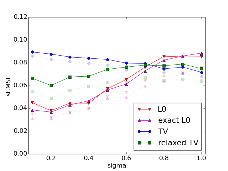
Figure 2 plots st.MSE comparisons for and . The estimate achieves significantly smaller risk than at higher signal-to-noise regimes, for example those displayed in Figure 1, while becomes competitive or better in lower signal-to-noise regimes, corresponding to lower values of normalized total-variation for the true signal. Figure 3 presents a different example to further explore this trade-off, in which the normalized total-variation of the signal is fixed at , and we increase the number of changepoints while simultaneously decreasing the jump sizes. (Changepoints are equally spaced, and distinct signal values are normally distributed.) The estimate is better under strong edge-sparsity, while becomes better as we transition to weaker edge-sparsity.
For the linear chain, we may compare with the exact minimizer of (L0) (computed using PELT in the changepoint R package [KFE12]). Algorithm 1 achieves risk comparable to the exact minimizer in all tested settings. One may ask, at the higher signal-to-noise regimes, how much of the sub-optimality of is due to estimator bias incurred by shrinkage. To address this, we computed also the “relaxed” TV estimate
where is an additional tuning parameter, and where replaces each constant interval of with the mean of over this interval. The error of at high signal-to-noise is partially reduced, but not to the same levels as .
6.4. 2-D lattice graph


Figure 4 displays a cartoon gray-scale image of a cow, represented by its pixel values on a 2-D lattice graph of size . Pure white corresponds to , and pure black to . The figure also displays and when the image is contaminated by noise at level . We again observe that oversmooths, missing details in the cow’s feet, right horn, and the shadows of the image. In contrast, undersmooths and returns a blotchy cow.
| sigma | 0.1 | 0.2 | 0.3 | 0.4 | 0.5 |
|---|---|---|---|---|---|
| st.MSE | 0.041 | 0.067 | 0.076 | 0.081 | 0.082 |
| (0.039) | (0.067) | (0.071) | (0.081) | (0.082) | |
| st.MSE | 0.083 | 0.075 | 0.065 | 0.061 | 0.054 |
| (0.083) | (0.075) | (0.065) | (0.059) | (0.053) |
6.5. Road and digital networks
We tested signal recovery over four real networks: the Oldenburg and San Francisco road networks from www.cs.utah.edu/~lifeifei/SpatialDataset.htm, and the Gnutella08 peer-to-peer network and Enron email network from snap.stanford.edu/data. Duplicate edges were removed, and only the largest connected component of each network was retained.
| Network | verts. | edges | res. var. | inf. | cut | inf. | cut | inf. | cut |
|---|---|---|---|---|---|---|---|---|---|
| Oldenburg | 6105 | 7029 | 0.118 | 57 | 16 | 515 | 75 | 2108 | 164 |
| San Fran. | 174956 | 221802 | 0.203 | 8574 | 306 | 27724 | 562 | 70925 | 774 |
| Gnutella | 6299 | 20776 | 0.826 | 19 | 91 | 67 | 477 | 271 | 3894 |
| Enron | 33696 | 180811 | 1.297 | 179 | 7319 | 2564 | 74117 | 16868 | 29253 |


For each network, we simulated an epidemic according to a simple graph-based discrete-time SI model [MN00], randomly selecting a source vertex to infect at time and, for each of timesteps, allowing each infected vertex to independently infect each non-infected neighbor with probability 0.5. We associated the values and to infected and non-infected vertices. For each network, we considered three signals corresponding to observations of the epidemic at three different times . Various properties of these networks and signals are summarized in Table 3.


For noise level , the simulated signal, , and computed with effective-resistance edge weights are depicted in Figure 6 for the San Francisco road network at observation time . The most difficult regions to estimate are the signal boundaries; we zoom in on three regions of the map where is inaccurate at these boundaries, but is mostly correct. At this noise level, the st.MSE of exceeds by a factor of about 2.
Figure 5 displays st.MSE comparisons for , , and with effective-resistance weighting at noise levels to in each example. We observe that is not substantially worse than in any tested setting, and that in the Gnutella and Enron digital networks where there is large variation in effective edge resistances, is sometimes substantially better. At the tested noise levels, these methods are (with the exception of Enron ) not substantially worse than , and can be substantially better in the lower noise settings.
7. Conclusion
We have studied estimation of piecewise-constant signals over arbitrary graphs using an edge penalty, establishing minimax rate-optimal statistical guarantees for the local minimizer computed by an approximation algorithm for minimizing this objective. We have shown theoretically that the same guarantees are not necessarily achieved by total-variation denoising, and empirically that -penalization may be more effective in high signal-to-noise settings. For application to networks with regions of varying connectivity, we have proposed minimization of an edge-weighted objective, which achieves better empirical performance in tested examples and leads to theoretical guarantees that are spatially uniform over all graphs.
We note that while Algorithm 1 is provably polynomial-time, discretization of the continuous parameter domain yields poor worst-case runtime and may be computationally costly to extend to likelihood models with multi-dimensional parameters. The development of faster non-discretized algorithms is an interesting direction for future work. Finally, our problem may be reformulated as sparse regression with particular graph-based designs, and we believe it is an interesting question whether similar computational ideas may be used to achieve better prediction error in sparse regression for more general families of designs.
Appendix A Properties of Algorithm 1
Proof of Proposition 2.2.
The initial objective value is . This value decreases by at least in each outer loop of Algorithm 1, so there are at most outer iterations. Within each outer iteration, there are at most inner loop iterations. The augmented graph of Algorithm 2 has vertices and edges, so solving minimum s-t cut using either Edmonds-Karp or Dinic’s algorithm requires time . This is the dominant cost of Algorithm 2, so combining these runtimes yields the proposition. ∎
Proof of Proposition 2.3.
The objective (W) may be written as
and each edge-cost satisfies the triangle inequality in the sense
for any . Hence, the first statement follows from Theorem 5.4 and Corollary 5.5 of [BVZ01]. Termination of the algorithm implies that for every -expansion of with new value , and hence also for every new value . Then is a -local-minimizer. ∎
Appendix B Analysis of weighted -denoising
In this appendix, we prove Theorems 5.4, 5.5, and 5.8. Recall from the end of Section 5 that these imply, as direct corollaries, Theorems 3.1, 3.2, 3.3, and 3.5. By rescaling, we will assume without loss of generality that .
Terminology.
A multi-cut of is a partition of its vertices into non-empty disjoint vertex subsets , which are called the elements of the multi-cut. In this appendix, we do not require each element of to be connected in . The multi-cut is trivial if , i.e. its only element is the entire vertex set . For two multi-cuts and , is a refinement of if this holds in the usual sense of partitions: For every element of , there exists an element of that contains as a subset. For any two multi-cuts and , their least common refinement is denoted by .
For every , the multi-cut induced by is such that any two vertices are in the same element of the cut if and only if . (If is constant on , then it induces the trivial multi-cut.) A multi-cut cuts an edge if and belong to two different elements. The set of all cut edges of , i.e. the boundary of the multi-cut, is denoted
( is empty if is trivial.) Recall for any . It is then evident that if induces , then
Associated to each multi-cut is a -dimensional subspace , such that if and only if takes a constant value on each element . (I.e., if and only if is equal to, or is a refinement of, the multi-cut induced by .) We denote the orthogonal projection onto by .
We first recall a deterministic sub-optimality bound for any -local-minimizer of (W). Such a bound was stated in [BVZ01] as a factor-2 approximation, , where is any -local-minimizer of (W) and is the exact minimizer in . In fact, this factor of 2 applies only to the penalty term, the resulting bound holds not only for but also for any , and it is easily extended to any . The proof is essentially the same, and we provide it here for completeness.
Lemma B.1.
Let and , and let be any -local-minimizer of in (W). Then for any vector whose entries take distinct values,
Proof.
Let be the multi-cut induced by . Fix and denote by the (constant) value of on . Let be the -expansion of defined entrywise by
Since is a -local-minimizer of (W), by definition
As for , we may cancel terms from both sides to yield
For the right side above, note that when , and apply the trivial bound when , i.e. when is cut by . Then, summing the above over ,
where the second line follows from noting that each edge cut by appears twice in the sum. The desired result then follows by noting that each edge appears at least once in the double sum on the left side. ∎
Next, we control using the weighted cut-size uniformly over all multi-cuts of . As the number of distinct multi-cuts of may be very large, we will first condition on a random spanning tree of , consider the common refinement of those multi-cuts that cut the same set of edges of , and take a union bound over these refinements. The distribution of the random spanning tree that we take is the one specified by the edge-weighting such that .
Lemma B.2.
Let be such that for some , and let have coordinates . Then there exist universal constants such that with probability at least , for every multi-cut of ,
Proof.
If is the trivial multi-cut consisting of the single element , then and , so with probability at least by a standard Gaussian tail bound.
Consider, then, non-trivial multi-cuts . By (13), . Observe that for any , the function is increasing over . Then, as ,
and it suffices to establish the stronger bound given by the right side above.
For any , we may bound
where the suprema are over all non-trivial multi-cuts of . Corresponding to the weighting is a distribution over random spanning trees of , satisfying the property (11). Let and denote the expectations over and over . Then the above yields
Observe that for any , is concave over , so is convex over . Also, . Then applying Jensen’s inequality,
| (17) |
Fix , and note that for any non-trivial multi-cut . We now control the supremum over by a union bound over all possible non-empty edge sets :
Consider any fixed non-empty subset , and denote by the multi-cut obtained in the following way: Remove the edges from , and let the elements of be the remaining connected components in the graph with edges . If is any other multi-cut satisfying , then any two vertices in the same element of are connected by a path of edges in that are not cut by , and hence these vertices belong to the same element of . Thus is a refinement of . Then the range of the projection is a linear subspace of the range of , and we consequently have (deterministically for any ). Then
has elements, so . Then for , the chi-squared moment-generating-function yields , so
Applying for every spanning tree ,
Fixing to be a constant (say ), it is easily verified that for , the function
is convex, so its maximum over is attained at either or . Thus
for sufficiently large constants , as desired. ∎
The preceding two lemmas yield risk bounds for in probability via a standard Cauchy-Schwarz argument, see e.g. [BM01, Theorem 2].
Lemma B.3.
Let and , and let be such that for some .
- (a)
For any , there exist constants depending only on such that for any true signal , any (fixed) , and any , with probability at least all -local-minima of (W) satisfy
- (b)
There exist universal constants such that for any , any true signal with , and any , with probability at least all -local-minima of (W) satisfy
Proof.
For part (a), let be the vector obtained by rounding each entry of to the nearest value in , and let be any -local-minimizer. Recall that if the entries of take distinct values, then by (13). Then by Lemma B.1,
Writing and canceling from both sides,
| (18) |
Suppose induces the multi-cut of , and induces the multi-cut of . Denote by the least common refinement of and , so
For any positive constants such that and , applying and yields
Applying this to (18) and rearranging yields
| (19) |
Finally, we obtain bounds in expectation by applying Hölder’s inequality and a crude bound on the th power of the squared-error risk for some .
Lemma B.4.
Let , , and be any -local-minimizer of (W). Then for any , there exists a constant depending only on such that
Proof.
Let denote the vector obtained by rounding each entry of to the nearest value in . For each vertex , the vector obtained by replacing with and keeping all other coordinates of the same is a -expansion of . Since is a -local-minimizer, this implies and hence (cancelling terms not depending on the th coordinate)
Summing over and applying ,
Then, applying ,
for a constant . Since , this implies
for a different constant . ∎
Proof of Theorem 5.4.
For and , denote
Note that whenever , , and . Applying Hölder’s inequality and Lemma B.3(a), there exist constants such that for any , any , and any constants such that ,
Note that , so for any . Then, choosing , , and applying Lemma B.4,
for a constant . Taking the infimum over yields the desired result. ∎
Proof of Theorem 5.5.
The proof of the upper bound is the same as that of Theorem 5.4, using Lemma B.3(b) instead of Lemma B.3(a): For universal constants , any , , , and and ,
For the lower bound, denote , and consider the vertex subset . Then the class contains the class of sparse vectors
where denotes the set of vertices for which . (This is because for any , .) Then
For , the lower-bound for the sparse normal-means problem (see e.g. Theorem 1(b) of [RWY11] in the case ) yields, for a universal constant ,
Note that for all , so
Then , and the lower bound follows. ∎
Proof of Theorem 5.8.
Let denote the (constant) vector obtained by rounding the value in to the closest value in . As is a -expansion of , and is a -local-minimizer, we have
Denoting by the multi-cut induced by , the same steps as leading to (19) yield, for any positive constants and such that ,
Hence, for and ,
for a constant . Lemma B.2 implies, with probability at least ,
Recall by (13) that if . Thus, if , then the above two statements imply , and hence is constant with probability at least , as desired. ∎
Appendix C Total-variation lower bound for the linear chain
In this appendix, we prove Theorems 4.1 and 4.2. By rescaling, we will assume . We say that consecutive intervals partition if there are integers such that for each . We associate to each such partition two orthogonal projections and , such that projects onto the -dimensional subspace of vectors assuming a constant value on each , and projects onto the -dimensional orthogonal complement of this subspace. More formally, for each and each , is defined by , and . We denote by the range of , and for any we denote by the (constant) value of over .
We will say that induces such a partition and a sign vector if and for each . Recall the vertex-edge incidence matrix : In this appendix, for the linear chain graph, let us fix the sign convention for so that .
The following lemma is an implication of the subgradient condition for minimizing (TV); a similar result was stated as Lemmas 2.1 and A.1 of [Rin09].
Lemma C.1.
Let . Fix consecutive intervals that partition , and fix a sign vector . Define such that, for each ,
| (21) |
where we set . Define also
Then the following two events are equivalent:
- (1)
The minimizer of (TV) induces the partition and the signs .
- (2)
and .
Furthermore, if this event holds, then .
Proof.
Suppose minimizes (TV) and induces and . Then is precisely the subdifferential of the -norm at , so is the subdifferential of with respect to . Since minimizes (TV), it satisfies the subgradient condition . Apply to both sides, noting that and for any . Then . Since induces the signs , we have . Also, , as desired.
Using this characterization, we may lower-bound the number of intervals in the partition induced by when the true signal is 0:
Proof of Theorem 4.1(a).
For a fixed partition into consecutive intervals, let us first bound
Denoting by the Euclidean unit ball in centered at 0, clearly
The range of is the -dimensional space orthogonal to the all-1’s vector, and is a projection onto an -dimensional subspace of this range—hence has rank . Let denote the (reduced) singular value decomposition of , where contains the singular values , and and have orthonormal columns. Then, as , we have
The set is an ellipsoid in , whose principal axes are aligned with the standard basis and have lengths . The vector of length has i.i.d. entries distributed as (when .) Then, for any , letting denote the first coordinates of and denote the projection of onto the first dimensions,
Here, denotes the volume in , and we have used . Note, by Cauchy interlacing, that where denotes the smallest non-zero singular value of . (Equality holds if the directions in the column span of that are projected out by are exactly those corresponding to the smallest non-zero singular values of .) As is the Laplacian of the linear chain graph, which has non-zero eigenvalues for [AJM85], this implies and hence, for any ,
Applying the Gamma function duplication formula , and , this yields
| (22) |
Fix . Suppose induces the partition having elements, and . Then Lemma C.1 implies , where and are defined in terms of and . Applying to both sides and noting ,
Thus there exists some partition into exactly consecutive intervals (equal to or refining ) for which applying to both sides above yields . As there are such partitions, applying a union bound, (22), and for any (see Theorem 1.5 of [Bat08]),
Taking ensures , and taking for a sufficiently small constant then ensures , for constants , as desired. ∎
To show part (b) of Theorem 4.1, we will argue that on the event where induces a partition into at least intervals, the squared-error of is typically also at least (up to logarithmic factors). We establish this using the next two lemmas.
Suppose that induces the partition and the signs . For any , let us call a local maximum interval if and , and a local minimum interval if and , where by convention .
Lemma C.2.
Let , let be the minimizer of (TV), and suppose is such that . There exists a constant such that with probability at least , every local minimum interval and local maximum interval of the partition and signs induced by has length at least .
Proof.
For any and any interval , denote . Define the event
By a Gaussian tail bound and union bound, .
Let be the partition into consecutive intervals induced by . Define
Consider corresponding to the smallest length . Let be the element immediately before or after in , and note that if is a local maximum, then is a local minimum, and vice versa. Then, letting be as defined in (21), exceeds by , so we must have
On the event ,
where the last bound recalls that has smallest length among . Then on ,
which implies
∎
Lemma C.3.
Fix any . Let be a random vector distributed as , and let be any convex cone with vertex 0 and non-empty interior. Then there exists a universal constant such that
Proof.
Consider a change of variables to and a set of angular variables representing the angle of . Since is a cone with vertex 0, the condition is a function only of . Hence the joint density of and conditional on is given by
for some quantity independent of . Note that for any and any ,
Letting denote a positive random variable with density function
where is the normalization constant such that , this implies . Integrating over and denoting by the marginal distribution of conditional on , this implies . The inequality is reversed for , so
That is, the distribution of conditional on stochastically dominates the (unconditional) distribution of .
Thus, to conclude the proof of the lemma, it suffices to lower bound
where is the moment of the distribution truncated on the left at 0. Integration by parts yields the recurrence , and Cauchy-Schwarz yields . Then
so
and the result follows by taking the square. ∎
Proof of Theorem 4.1(b).
For any positive constant , it suffices to consider graphs with . (For , the lower bound trivially holds by adjusting based on , as the risk is clearly non-zero for any graph.)
Let induce the partition and signs . For any fixed partition and signs , by Lemma C.1,
where , , and are fixed and defined by and . Since the projections and are orthogonal to each other, is independent of , so we may drop the conditioning on the event . Define by for each , where . Then , for , and the condition is equivalent to for some convex cone with vertex 0 and non-empty interior. Applying Lemma C.3, for a constant ,
| (23) |
Let , , and denote , , and as defined above for the random induced partition and signs and . By part (a) of this theorem (already established), for some constant and any , on an event of probability at least , . Note that is only non-zero on those intervals which are local maxima or local minima, and that the (constant) value of on any such interval has magnitude at most . Applying Lemma C.2 with , on a different event of probability at least , every local minimum and local maximum interval of has length . (For this statement is trivial.) Then, on this event, there are at most such intervals, and hence
Taking the full expectation of (23) over the intersection of these two events of probability at least , the theorem follows. ∎
Proof of Theorem 4.2.
Let denote the constant in Lemma C.2. If
then the lower bound follows from Theorem 4.1(b) by considering the risk at . Otherwise, construct a signal by the following procedure:
- (1)
Choose
disjoint intervals in , each of length .
- (2)
Set . For each , divide into three sub-intervals of length , and set for each belonging to the middle such sub-interval.
- (3)
Set for all remaining indices.
This signal satisfies and . We have
so Lemma C.2 implies that on an event of probability at least , every local maximum or local minimum interval for the partition and signs induced by has length at least . On this event , there cannot be a sub-interval of any that is a local maximum or local minimum, so the estimate must be monotonically increasing or monotonically decreasing over each interval . Then it is easily verified that
for constants , where the last inequality uses and . The result follows upon taking the expectation over . ∎
Acknowledgments
We would like to thank Professors Amin Saberi, James Sharpnack, and Emmanuel Candes for helpful and inspiring discussions on this problem and related literature.
References
- [ABBDL10] Louigi Addario-Berry, Nicolas Broutin, Luc Devroye, and Gábor Lugosi. On combinatorial testing problems. Ann. Statist., 38(5):3063–3092, 2010.
- [ACCD11] Ery Arias-Castro, Emmanuel J Candès, and Arnaud Durand. Detection of an anomalous cluster in a network. Ann. Statist., 39(1):278–304, 2011.
- [ACCHZ08] Ery Arias-Castro, Emmanuel J Candès, Hannes Helgason, and Ofer Zeitouni. Searching for a trail of evidence in a maze. Ann. Statist., 36(4):1726–1757, 2008.
- [ACDH05] Ery Arias-Castro, David L Donoho, and Xiaoming Huo. Near-optimal detection of geometric objects by fast multiscale methods. IEEE Trans. Inform. Theory, 51(7):2402–2425, 2005.
- [ACG13] Ery Arias-Castro and Geoffrey R Grimmett. Cluster detection in networks using percolation. Bernoulli, 19(2):676–719, 2013.
- [AJM85] William N Anderson Jr and Thomas D Morley. Eigenvalues of the Laplacian of a graph. Linear Multilinear Algebra, 18(2):141–145, 1985.
- [AL89] Ivan E Auger and Charles E Lawrence. Algorithms for the optimal identification of segment neighborhoods. Bull. Math. Biol., 51(1):39–54, 1989.
- [Bat08] Necdet Batir. Inequalities for the gamma function. Arch. Math. (Basel), 91(6):554–563, 2008.
- [BBM99] Andrew Barron, Lucien Birgé, and Pascal Massart. Risk bounds for model selection via penalization. Probab. Theory Related Fields, 113(3):301–413, 1999.
- [Bes86] Julian Besag. On the statistical analysis of dirty pictures. J. R. Stat. Soc. Ser. B. Stat. Methodol., 48(3):259–302, 1986.
- [BH93] Daniel Barry and John A Hartigan. A Bayesian analysis for change point problems. J. Amer. Statist. Assoc., 88(421):309–319, 1993.
- [BK04] Yuri Boykov and Vladimir Kolmogorov. An experimental comparison of min-cut/max-flow algorithms for energy minimization in vision. IEEE Trans. Pattern Anal. Mach. Intell., 26(9):1124–1137, 2004.
- [BKL+09] Leif Boysen, Angela Kempe, Volkmar Liebscher, Axel Munk, and Olaf Wittich. Consistencies and rates of convergence of jump-penalized least squares estimators. Ann. Statist., 37(1):157–183, 2009.
- [BM01] Lucien Birgé and Pascal Massart. Gaussian model selection. J. Euro. Math. Soc., 3(3):203–268, 2001.
- [BM07] Lucien Birgé and Pascal Massart. Minimal penalties for Gaussian model selection. Probab. Theory Related Fields, 138(1-2):33–73, 2007.
- [BRT09] Peter J Bickel, Ya’acov Ritov, and Alexandre B Tsybakov. Simultaneous analysis of Lasso and Dantzig selector. Ann. Statist., 37(4):1705–1732, 2009.
- [BVZ01] Yuri Boykov, Olga Veksler, and Ramin Zabih. Fast approximate energy minimization via graph cuts. IEEE Trans. Pattern Anal. Mach. Intell., 23(11):1222–1239, 2001.
- [CDS01] Scott Shaobing Chen, David L Donoho, and Michael A Saunders. Atomic decomposition by basis pursuit. SIAM Rev., 43(1):129–159, 2001.
- [Cha05] Antonin Chambolle. Total variation minimization and a class of binary MRF models. In EMMCVPR, volume 5, pages 136–152. Springer, 2005.
- [CL97] Antonin Chambolle and Pierre-Louis Lions. Image recovery via total variation minimization and related problems. Numer. Math., 76(2):167–188, 1997.
- [CZ64] Herman Chernoff and Shelemyahu Zacks. Estimating the current mean of a normal distribution which is subjected to changes in time. Ann. Math. Statist., 35(3):999–1018, 1964.
- [DHL17] Arnak S Dalalyan, Mohamed Hebiri, and Johannes Lederer. On the prediction performance of the Lasso. Bernoulli, 23(1):552–581, 2017.
- [DJ94] David L Donoho and Iain M Johnstone. Ideal spatial adaptation by wavelet shrinkage. Biometrika, 81(3):425–455, 1994.
- [DK01] P Laurie Davies and Arne Kovac. Local extremes, runs, strings and multiresolution. Ann. Statist., 29(1):1–48, 2001.
- [Don99] David L Donoho. Wedgelets: Nearly minimax estimation of edges. Ann. Statist., 27(3):859–897, 1999.
- [DS05] Jérôme Darbon and Marc Sigelle. A fast and exact algorithm for total variation minimization. In Iberian Conference on Pattern Recognition and Image Analysis, pages 351–359. Springer, 2005.
- [Efr04] Bradley Efron. Large-scale simultaneous hypothesis testing: the choice of a null hypothesis. J. Amer. Statist. Assoc., 99(465):96–104, 2004.
- [GBS08] Arpita Ghosh, Stephen Boyd, and Amin Saberi. Minimizing effective resistance of a graph. SIAM Rev., 50(1):37–66, 2008.
- [GG84] Stuart Geman and Donald Geman. Stochastic relaxation, Gibbs distributions, and the Bayesian restoration of images. IEEE Trans. Pattern Anal. Mach. Intell., 6:721–741, 1984.
- [GLCS17] Adityanand Guntuboyina, Donovan Lieu, Sabyasachi Chatterjee, and Bodhisattva Sen. Spatial adaptation in trend filtering. arXiv:1702.05113, 2017.
- [GO09] Tom Goldstein and Stanley Osher. The split Bregman method for L1-regularized problems. SIAM J. Imaging Sci., 2(2):323–343, 2009.
- [GPS89] Dorothy M Greig, Bruce T Porteous, and Allan H Seheult. Exact maximum a posteriori estimation for binary images. J. R. Stat. Soc. Ser. B. Stat. Methodol., 51(2):271–279, 1989.
- [Har16] Xiaoying Tian Harris. Prediction error after model search. arXiv:1610.06107, 2016.
- [HLL10] Zaıd Harchaoui and Céline Lévy-Leduc. Multiple change-point estimation with a total variation penalty. J. Amer. Statist. Assoc., 105(492):1480–1493, 2010.
- [HMPSST16] Oscar Hernan Madrid Padilla, James G Scott, James Sharpnack, and Ryan J Tibshirani. The DFS fused lasso: nearly optimal linear-time denoising over graphs and trees. arXiv:1608.03384, 2016.
- [Hoe10] Holger Hoefling. A path algorithm for the fused lasso signal approximator. J. Comput. Graph. Statist., 19(4):984–1006, 2010.
- [HR16] Jan-Christian Hütter and Philippe Rigollet. Optimal rates for total variation denoising. In Conf. Learning Theory, pages 1115–1146, 2016.
- [Joh15] Iain Johnstone. Gaussian estimation: Sequence and wavelet models. Available at statweb.stanford.edu/ imj/GE09-08-15.pdf, 2015.
- [JS+05] Brad Jackson, Jeffrey D Scargle, et al. An algorithm for optimal partitioning of data on an interval. IEEE Signal Process. Lett., 12(2):105–108, 2005.
- [KFE12] Rebecca Killick, Paul Fearnhead, and Idris A Eckley. Optimal detection of changepoints with a linear computational cost. J. Amer. Statist. Assoc., 107(500):1590–1598, 2012.
- [KS96] David R Karger and Clifford Stein. A new approach to the minimum cut problem. Journal of the ACM (JACM), 43(4):601–640, 1996.
- [KS11] Arne Kovac and Andrew DAC Smith. Nonparametric regression on a graph. J. Comput. Graph. Statist., 20(2):432–447, 2011.
- [KT93] Aleksandr Petrovich Korostelev and Alexandre B Tsybakov. Minimax theory of image reconstruction, volume 82. Springer Science & Business Media, 1993.
- [KZ04] Vladimir Kolmogorov and Ramin Zabin. What energy functions can be minimized via graph cuts? IEEE Trans. Pattern Anal. Mach. Intell., 26(2):147–159, 2004.
- [L93] Lovász L. Random walks on graphs: A survey. Combinatorics, Paul Erdös is eighty, 2:1–46, 1993.
- [LB12] Oren E Livne and Achi Brandt. Lean algebraic multigrid (LAMG): Fast graph Laplacian linear solver. SIAM J. Sci. Comput., 34(4):B499–B522, 2012.
- [Leb05] Émilie Lebarbier. Detecting multiple change-points in the mean of Gaussian process by model selection. Signal processing, 85(4):717–736, 2005.
- [LF97] Stephanie R Land and Jerome H Friedman. Variable fusion: A new adaptive signal regression method. Technical report, 656, Department of Statistics, Carnegie Mellon University, 1997.
- [LSRT16] Kevin Lin, James Sharpnack, Alessandro Rinaldo, and Ryan J Tibshirani. Approximate recovery in changepoint problems, from estimation error rates. arXiv:1606.06746, 2016.
- [MN00] Cristopher Moore and Mark EJ Newman. Epidemics and percolation in small-world networks. Phys. Rev. E, 61(5):5678, 2000.
- [MS89] David Mumford and Jayant Shah. Optimal approximations by piecewise smooth functions and associated variational problems. Comm. Pure Appl. Math., 42(5):577–685, 1989.
- [MvdG97] Enno Mammen and Sara van de Geer. Locally adaptive regression splines. Ann. Statist., 25(1):387–413, 1997.
- [Rin09] Alessandro Rinaldo. Properties and refinements of the fused lasso. Ann. Statist., 37(5B):2922–2952, 2009.
- [ROF92] Leonid I Rudin, Stanley Osher, and Emad Fatemi. Nonlinear total variation based noise removal algorithms. Phys. D, 60(1-4):259–268, 1992.
- [RWY11] Garvesh Raskutti, Martin J Wainwright, and Bin Yu. Minimax rates of estimation for high-dimensional linear regression over -balls. IEEE Trans. Inform. Theory, 57(10):6976–6994, 2011.
- [SKS13] James L Sharpnack, Akshay Krishnamurthy, and Aarti Singh. Near-optimal anomaly detection in graphs using lovasz extended scan statistic. In Adv. Neural Inform. Process. Syst., pages 1959–1967, 2013.
- [SRS12] James Sharpnack, Alessandro Rinaldo, and Aarti Singh. Sparsistency of the edge lasso over graphs. In Int. Conf. Artific. Intell. Statist., pages 1028–1036, 2012.
- [SS11] Daniel A Spielman and Nikhil Srivastava. Graph sparsification by effective resistances. SIAM J. Comput., 40(6):1913–1926, 2011.
- [SSR13] James Sharpnack, Aarti Singh, and Alessandro Rinaldo. Detecting activations over graphs using spanning tree wavelet bases. In Int. Conf. Artific. Intell. Statist., pages 545–553, 2013.
- [ST04] Daniel A Spielman and Shang-Hua Teng. Nearly-linear time algorithms for graph partitioning, graph sparsification, and solving linear systems. In ACM Symp. Theory Comput., pages 81–90. ACM, 2004.
- [SWT16a] Veeranjaneyulu Sadhanala, Yu-Xiang Wang, and Ryan J Tibshirani. Total variation classes beyond 1d: Minimax rates, and the limitations of linear smoothers. In Adv. Neural Inform. Process. Syst., pages 3513–3521, 2016.
- [SWT16b] Veeru Sadhanala, Yu-Xiang Wang, and Ryan Tibshirani. Graph sparsification approaches for Laplacian smoothing. In Int. Conf. Artific. Intell. Statist., pages 1250–1259, 2016.
- [Tib96] Robert Tibshirani. Regression shrinkage and selection via the lasso. J. R. Stat. Soc. Ser. B. Stat. Methodol., 58(1):267–288, 1996.
- [TS15] Wesley Tansey and James G Scott. A fast and flexible algorithm for the graph-fused lasso. arXiv:1505.06475, 2015.
- [TSR+05] Robert Tibshirani, Michael Saunders, Saharon Rosset, Ji Zhu, and Keith Knight. Sparsity and smoothness via the fused lasso. J. R. Stat. Soc. Ser. B. Stat. Methodol., 67(1):91–108, 2005.
- [TT11] Ryan J Tibshirani and Jonathan Taylor. The solution path of the generalized lasso. Ann. Statist., 39(3):1335–1371, 2011.
- [TT15] Xiaoying Tian and Jonathan E Taylor. Selective inference with a randomized response. arXiv:1507.06739, 2015.
- [VDGB09] Sara A Van De Geer and Peter Bühlmann. On the conditions used to prove oracle results for the Lasso. Electron. J. Stat., 3:1360–1392, 2009.
- [WL02] Gerhard Winkler and Volkmar Liebscher. Smoothers for discontinuous signals. J. Nonparametr. Stat., 14(1-2):203–222, 2002.
- [WSST16] Yu-Xiang Wang, James Sharpnack, Alex Smola, and Ryan J Tibshirani. Trend filtering on graphs. J. Mach. Learn. Res., 17(105):1–41, 2016.
- [XKWG14] Bo Xin, Yoshinobu Kawahara, Yizhou Wang, and Wen Gao. Efficient generalized fused lasso and its application to the diagnosis of Alzheimer’s disease. In Proc. Assoc. Adv. Artific. Intell. Conf., pages 2163–2169, 2014.
- [YA89] Yi-Ching Yao and Siu-Tong Au. Least-squares estimation of a step function. Sankhya A, 51(3):370–381, 1989.
- [Yao84] Yi-Ching Yao. Estimation of a noisy discrete-time step function: Bayes and empirical Bayes approaches. Ann. Statist., 12(3):1434–1447, 1984.
- [Yao88] Yi-Ching Yao. Estimating the number of change-points via Schwarz’ criterion. Statist. Probab. Lett., 6(3):181–189, 1988.
- [ZWJ14] Yuchen Zhang, Martin J Wainwright, and Michael I Jordan. Lower bounds on the performance of polynomial-time algorithms for sparse linear regression. In Conf. Learning Theory, volume 35, pages 1–28, 2014.
- [ZWJ17] Yuchen Zhang, Martin J Wainwright, and Michael I Jordan. Optimal prediction for sparse linear models? Lower bounds for coordinate-separable M-estimators. Electron. J. Stat., 11(1):752–799, 2017.