跳到论文正文
W Papers独立论文阅读器 arXiv:1703.01395 论文正文 计算阅读时间 · 0%
引用这篇论文根据当前论文元数据生成,正式投稿前建议核对。


License: arXiv.org perpetual non-exclusive license
arXiv:1703.01395v1 [math.QA] 04 Mar 2017

Dual wavefunction of the symplectic ice

Kohei Motegi ††thanks: E-mail: kmoteg0@kaiyodai.ac.jp Affiliation: Faculty of Marine Technology, Tokyo University of Marine Science and Technology, Affiliation: Etchujima 2-1-6, Koto-Ku, Tokyo, 135-8533, Japan
August 24, 2026
Abstract

The wavefunction of the free-fermion six-vertex model was found to give a natural realization of the Tokuyama combinatorial formula for the Schur polynomials by Bump-Brubaker-Friedberg. Recently, we studied the correspondence between the dual version of the wavefunction and the Schur polynomials, which gave rise to another combinatorial formula. In this paper, we extend the analysis to the reflecting boundary condition, and show the exact correspondence between the dual wavefunction and the symplectic Schur functions. This gives a dual version of the integrable model realization of the symplectic Schur functions by Ivanov. We also generalize to the correspondence between the wavefunction, the dual wavefunction of the six-vertex model and the factorial symplectic Schur functions by the inhomogeneous generalization of the model.

Mathematics Subject Classification. 05E05, 05E10, 16T25, 16T30, 17B37.

Keywords. Integrable lattice models, Yang-Baxter equation, Symmetric functions, Combinatorial representation theeory.

1 Introduction

The study of the connections between integrable lattice models [1, 2, 3, 4] and combinatorial representation theory of symmetric polynomials is an active area of research in these years.

The main actor is the wavefunction in this research, which is constructed from the RR-matrices satisfying the Yang-Baxter relation. The wavefunction of the most famous six-vertex model [5, 6] whose RR-matrix comes from the Drinfeld-Jimbo quantum group [7, 8] Uq​(s​l2)U_{q}(sl_{2}) representation, and its q=0q=0 five-vertex model degeneration, has turned out to give a representation of the Grothendieck polynomials and its quantum group deformation (see [9, 10, 11, 12, 13, 14, 15, 16, 17] for example). Based on this correspondence, various algebraic combinatorial identities have been discovered and proved. It seems that many of the identities themselves are hard to be discovered without the power of quantum integrability. These developments may shed new light in the world of Schubert calculus [18, 19, 20, 21, 22, 23, 24, 25]. For example, the notion of excited Young diagram [21] in the field of Schubert calculus is essentially equivalent to the wavefunction of certain integrable five-vertex models. Translating into the language of quantum integrable models can give new insights. For example, there is a recent development on the investigation of the Littlewood-Richardson coefficients from the point of view of quantum integrability [13].

The object treated in this paper is based on another way of direction of the developments uncovered by number theorists. Bump, Brubaker and Friedberg found [26] that a ceratin kind of free-fermion six-vertex model gives a natural realization of the Tokuyama formula [27], which gives a deformation of the Weyl character formula. The free-fermion six-vertex model can be regarded as a gauge-deformed version of the Felderhof free-fermion model [28], whose underlying quantum group symmetry can be explained either as an exotic roots of unity finite-dimensional highest weight representation [29, 30]. Another explanation is that the free-fermion six-vertex model corresponds to the simplest case of the Perk-Schultz model [31] which is a representation of quantum supergroup. The latter formulation recently gave rise to the Yang-Baxter equation [32] for the metaplectic ice [33]. As for the domain wall boundary partition function which is a special class of partition functions, it was evaluated in [34, 35] by using the Izergin-Korepin technique in the past and factorization phenomena was observed.

However, it was only found in recent years that the free-fermion model has rich mathematical structures related with the combinatorial representation theory of Schur polynomials. One of the striking facts found [26] was that the Tokuyama formula [27], which is a one-parameter deformation of the Weyl character formula, is naturally realized as the wavefunction of the free-fermion model. The wavefunction is the most fundamental object in the statistical physical aspects of quantum integrable models, since it becomes the Bethe eigenvectors of the corresponding one-dimensional spin chain when the Bethe ansatz equation is imposed on the spectral parameters.

The Tokuyama formula for the Schur polynomials can be understood as a consequence of the evaluation of the wavefunction in two ways. One by expressing it as a product of a one-parameter deformation of the Vandermonde determinant and the Schur polynomials, and another one by making a microscopic analysis and deirve an expression using the strict Gelfand-Tsetlin pattern. The Tokuyama formula is a consequence of the two evaluations for the same object. This understanding [26] opened a new doorway to the combinatorial representation theory of symmetric polynomials via the free-fermion model. One of the progresses after this work is the construction of variations of the Tokuyamya-type formulas by changing boundary conditions. Several Tokuyama-type formulas for types other than type AA was obtained by Okada [36] and Hamel-King [37, 38] earlier, and recently by using methods of analytic number theory [39] and non-intersecting lattice paths [40, 41, 42].

They were investigated from the viewpoint of quantum integrability in [43, 44, 45, 46] where local objects and relations such as the LL-operators, KK-matrix and the Yang-Baxter relation are extensively used. For example, the correspondence between the wavefunction under the half-turn boundary condition and the symplectic Schur functions was obtained by Ivanov in [43].

On the other hand, we studied the dual wavefunction of the free-fermion model in a recent paper [47]. We gave the exact correspondence between the dual wavefunction and the Schur polynomials. which includes the special case t=1t=1 of the deformation parameter [26, 48], which was obtained by transforming the original wavefuncion to the dual wavefunction by symmetry arguments. We gave two proofs for the correspondence. One proof used transformation of the statement of the theorem to an equivalent statement so that one can use the arguments given in [26]. Another proof is a modern statistical mechanical approach, which combines the matrix product method [49, 50] and the Izergin-Korepin method of analysis on the domain wall boundary partition function [51, 52]. The exact correspondence with the Schur polynomials, together with a microscopic analysis of the dual wavefunction gave rise to a dual version of the Tokuyama-type formula for the Schur polynomials.

In this paper, we combine these two directions of progresses, and extend the study of the dual wavefunction to the free-fermion model under the reflecting boundary condition. We give the exact correspondence between the dual wavefunction and the symplectic Schur functions. We prove the correspondence by extending the argument used in the first proof in [47] to the reflecting boundary condition, so that one can use the arguments by Brubaker-Bump-Friedberg [26] and Ivanov [43]. This gives a dual version of type CC Tokuyama formula. We also generalize the Theorems by Ivanov and the main result in this paper to give the exact correspondence between the wavefunction, dual wavefunction and the factorial symplectic Schur functions by using two types of LL-operators and the KK-matrix of the inhomogeneous six-vertex model. This is a symplectic analogue of the work of Bump-McNamara-Nakasuji [48] which they established the Tokuyama-type formulas for factorial Schur functions. Recently, the Tokuyama-type formulas for factorial characters were obtained by using non-intersecting lattice paths by Hamel-King [41, 42] which is worthwhile to investigate the relation and the results in this paper in the future.

This paper is organized as follows. We introduce the free-fermion model in section 2 and review the relation between the wavefunction under the reflecting boundary condition and the symplectic Schur functions in section 3. In section 4, we introduce the dual wavefunction, and prove the relation with the symplectic Schur functions, which can be regarded as a dual version of type CC Tokuyama formula. In section 5, we generalize the correspondence and give the exact relation between the wavefuncion, dual wavefunction of the inhomogeneous free-fermion model and the factorial symplectic Schur functions. Section 6 is devoted to the conclusion.

2 Free-fermion model

We introduce the free-fermion model in this section, and review the results on the relation between the wavefunction and the symplectic Schur functions in the next section. We use the LL-operator in [26] which is best suited for the study of the combinatorics of the Schur polynomials, since the Tokuyama formula is exactly realized as the wavefunction constructed from this LL-operator. More generic or gauge-transformed ones can be found in [29, 30, 35] for example. We also use the terminology of the quantum inverse scattering method or the algebraic Bethe ansatz, which is one of the most fundamental methods for the analysis of quantum integrable models.

The most fundamental objects in integrable lattice models are the RR-matrix and the LL-operator. For the case of the free-fermion model we consider, the RR-matrix is given by

Ra​b​(z,t)=(1+t​z−10000t⁡(1−z−1)t+100(t+1)​z−1z−1−10000z−1+t),\displaystyle R_{ab}(z,t)=\left(\begin{array}[]{cccc}1+tz^{-1}&0&0&0\\ 0&t(1-z^{-1})&t+1&0\\ 0&(t+1)z^{-1}&z^{-1}-1&0\\ 0&0&0&z^{-1}+t\end{array}\right),

acting on the tensor product Wa⊗WbW_{a}\otimes W_{b} of the complex two-dimensional space WaW_{a}. Let us denote the orthonormal basis of WaW_{a} and its dual as {|0⟩a,|1⟩a}\{|0\rangle_{a},|1\rangle_{a}\} and {⟨0|,⟨1|}aa\{{}_{a}\langle 0|,{}_{a}\langle 1|\}, and the matrix elements of the RR-matrix as ⟨γ|⟨δ|Ra​b(z,t)|α⟩ab|β⟩ba=[Ra​b(z,t)]α​βγ​δ{}_{a}\langle\gamma|{}_{b}\langle\delta|R_{ab}(z,t)|\alpha\rangle_{a}|\beta\rangle_{b}=[R_{ab}(z,t)]_{\alpha\beta}^{\gamma\delta}. The matrix elements of the RR-matrix are explicitly given as

⟨0|⟨0|Ra​b(z,t)|0⟩ab|0⟩ba\displaystyle{}_{a}\langle 0|{}_{b}\langle 0|R_{ab}(z,t)|0\rangle_{a}|0\rangle_{b} =1+t​z−1,\displaystyle=1+tz^{-1}, (2.6)
⟨0|⟨1|Ra​b(z,t)|0⟩ab|1⟩ba\displaystyle{}_{a}\langle 0|{}_{b}\langle 1|R_{ab}(z,t)|0\rangle_{a}|1\rangle_{b} =t⁡(1−z−1),\displaystyle=t(1-z^{-1}), (2.7)
⟨0|⟨1|Ra​b(z,t)|1⟩ab|0⟩ba\displaystyle{}_{a}\langle 0|{}_{b}\langle 1|R_{ab}(z,t)|1\rangle_{a}|0\rangle_{b} =t+1,\displaystyle=t+1, (2.8)
⟨1|⟨0|Ra​b(z,t)|0⟩ab|1⟩ba\displaystyle{}_{a}\langle 1|{}_{b}\langle 0|R_{ab}(z,t)|0\rangle_{a}|1\rangle_{b} =(t+1)​z−1,\displaystyle=(t+1)z^{-1}, (2.9)
⟨1|⟨0|Ra​b(z,t)|1⟩ab|0⟩ba\displaystyle{}_{a}\langle 1|{}_{b}\langle 0|R_{ab}(z,t)|1\rangle_{a}|0\rangle_{b} =z−1−1,\displaystyle=z^{-1}-1, (2.10)
⟨1|⟨1|Ra​b(z,t)|1⟩ab|1⟩ba\displaystyle{}_{a}\langle 1|{}_{b}\langle 1|R_{ab}(z,t)|1\rangle_{a}|1\rangle_{b} =z−1+t.\displaystyle=z^{-1}+t. (2.11)

The LL-operator of the free-fermion model is given by

La​j​(z,t)=(10000t100(t+1)​z−1z−10000z−1),\displaystyle L_{aj}(z,t)=\left(\begin{array}[]{cccc}1&0&0&0\\ 0&t&1&0\\ 0&(t+1)z^{-1}&z^{-1}&0\\ 0&0&0&z^{-1}\end{array}\right),

acting on the tensor product Wa⊗ℱjW_{a}\otimes\mathcal{F}_{j} of the space WaW_{a} and the two-dimensional Fock space at the jjth site ℱj\mathcal{F}_{j}. We also denote the orthonormal basis of ℱj\mathcal{F}_{j} and its dual as {|0⟩j,|1⟩j}\{|0\rangle_{j},|1\rangle_{j}\} and {⟨0|,⟨1|}jj\{{}_{j}\langle 0|,{}_{j}\langle 1|\}, and the matrix elements of the LL-operator as ⟨γ|⟨δ|La​j(z,t)|α⟩aj|β⟩ja=[La​j(z,t)]α​βγ​δ{}_{a}\langle\gamma|{}_{j}\langle\delta|L_{aj}(z,t)|\alpha\rangle_{a}|\beta\rangle_{j}=[L_{aj}(z,t)]_{\alpha\beta}^{\gamma\delta}. The matrix elements of the LL-operator are explicitly written as (see Figure 1 for a pictorial description)

⟨0|⟨0|La​j(z,t)|0⟩aj|0⟩ja\displaystyle{}_{a}\langle 0|{}_{j}\langle 0|L_{aj}(z,t)|0\rangle_{a}|0\rangle_{j} =1,\displaystyle=1, (2.17)
⟨0|⟨1|La​j(z,t)|0⟩aj|1⟩ja\displaystyle{}_{a}\langle 0|{}_{j}\langle 1|L_{aj}(z,t)|0\rangle_{a}|1\rangle_{j} =t,\displaystyle=t, (2.18)
⟨0|⟨1|La​j(z,t)|1⟩aj|0⟩ja\displaystyle{}_{a}\langle 0|{}_{j}\langle 1|L_{aj}(z,t)|1\rangle_{a}|0\rangle_{j} =1,\displaystyle=1, (2.19)
⟨1|⟨0|La​j(z,t)|0⟩aj|1⟩ja\displaystyle{}_{a}\langle 1|{}_{j}\langle 0|L_{aj}(z,t)|0\rangle_{a}|1\rangle_{j} =(t+1)​z−1,\displaystyle=(t+1)z^{-1}, (2.20)
⟨1|⟨0|La​j(z,t)|1⟩aj|0⟩ja\displaystyle{}_{a}\langle 1|{}_{j}\langle 0|L_{aj}(z,t)|1\rangle_{a}|0\rangle_{j} =z−1,\displaystyle=z^{-1}, (2.21)
⟨1|⟨1|La​j(z,t)|1⟩aj|1⟩ja\displaystyle{}_{a}\langle 1|{}_{j}\langle 1|L_{aj}(z,t)|1\rangle_{a}|1\rangle_{j} =z−1.\displaystyle=z^{-1}. (2.22)

The RR-matrices and the LL-operators have origins in statistical physics, and |0⟩|0\rangle or its dual ⟨0|\langle 0| can be regarded as a hole state, while |1⟩|1\rangle or its dual ⟨1|\langle 1| can be interpretted as a particle state from the point of view of statistical physics. We use the terms hole states and particle states to describe states constructed from |0⟩|0\rangle, ⟨0|\langle 0|, |1⟩|1\rangle and ⟨1|\langle 1| from now on since they are convenient for the description of the states. We also remark that in the language of the quantum inverse scattering method, the Fock spaces WaW_{a} and ℱj\mathcal{F}_{j} are usually called as the auxiliary and quantum spaces, respectively.

Refer to caption
Figure 1: The first LL-operator (2). The (dual) state |0⟩|0\rangle (⟨0|\langle 0|) is represented as ⊕\oplus, while the (dual) state |1⟩|1\rangle (⟨1|\langle 1|) is represented as ⊖\ominus, following the pictorial description of [26].
Refer to caption
Figure 2: The second LL-operator (2). We follow the pictorial description of [43] for this second LL-operator.
Refer to caption
Figure 3: The KK-matrix (2). We follow the pictorial description of [43] for the KK-matrix.

The RR-matrix (2) and LL-operator (2) satsify the Yang-Baxter relation

Ra​b​(z1/z2,t)​La​j​(z1,t)​Lb​j​(z2,t)=Lb​j​(z2,t)​La​j​(z1,t)​Ra​b​(z1/z2,t),\displaystyle R_{ab}(z_{1}/z_{2},t)L_{aj}(z_{1},t)L_{bj}(z_{2},t)=L_{bj}(z_{2},t)L_{aj}(z_{1},t)R_{ab}(z_{1}/z_{2},t), (2.23)

acting on Wa⊗Wb⊗ℱjW_{a}\otimes W_{b}\otimes\mathcal{F}_{j}. We remark that this R​L​LRLL relation (2.23) can be regarded as a special case of the generalized Yang-Baxter relation for a more general RR-matrix [29, 30, 35]. The RR-matrix (2) and the LL-operator (2) in this section can be regarded as different specializations of the general RR-matrix from this viewpoint. One of the advantages of the point of view from the quantum group is that one can systematically generalize the Felderhof model to higher-dimensional representations [30].

To realize the Tokuyama formula for Schur polynomials, it was enough to use the LL-operator (2). To deal with symplectic Schur functions, one needs more objects. We introduce the second LL-operator (see Figure 2 )

L~a​j​(z,t)=(z0000t​z100(t+1)​z100001),\displaystyle\widetilde{L}_{aj}(z,t)=\left(\begin{array}[]{cccc}z&0&0&0\\ 0&tz&1&0\\ 0&(t+1)z&1&0\\ 0&0&0&1\end{array}\right),

whose matrix elements are explicitly given by

⟨0|⟨0|L~a​j(z,t)|0⟩aj|0⟩ja\displaystyle{}_{a}\langle 0|{}_{j}\langle 0|\widetilde{L}_{aj}(z,t)|0\rangle_{a}|0\rangle_{j} =z,\displaystyle=z, (2.29)
⟨0|⟨1|L~a​j(z,t)|0⟩aj|1⟩ja\displaystyle{}_{a}\langle 0|{}_{j}\langle 1|\widetilde{L}_{aj}(z,t)|0\rangle_{a}|1\rangle_{j} =t​z,\displaystyle=tz, (2.30)
⟨0|⟨1|L~a​j(z,t)|1⟩aj|0⟩ja\displaystyle{}_{a}\langle 0|{}_{j}\langle 1|\widetilde{L}_{aj}(z,t)|1\rangle_{a}|0\rangle_{j} =1,\displaystyle=1, (2.31)
⟨1|⟨0|L~a​j(z,t)|0⟩aj|1⟩ja\displaystyle{}_{a}\langle 1|{}_{j}\langle 0|\widetilde{L}_{aj}(z,t)|0\rangle_{a}|1\rangle_{j} =(t+1)​z,\displaystyle=(t+1)z, (2.32)
⟨1|⟨0|L~a​j(z,t)|1⟩aj|0⟩ja\displaystyle{}_{a}\langle 1|{}_{j}\langle 0|\widetilde{L}_{aj}(z,t)|1\rangle_{a}|0\rangle_{j} =1,\displaystyle=1, (2.33)
⟨1|⟨1|L~a​j(z,t)|1⟩aj|1⟩ja\displaystyle{}_{a}\langle 1|{}_{j}\langle 1|\widetilde{L}_{aj}(z,t)|1\rangle_{a}|1\rangle_{j} =1.\displaystyle=1. (2.34)

We also introduce the KK-matrix acting on the auxiliray space WaW_{a} (see Figure 3)

Ka​(z,t)=(t​z00z−1).\displaystyle K_{a}(z,t)=\left(\begin{array}[]{cc}tz&0\\ 0&z^{-1}\\ \end{array}\right).

The KK-matrix is used when partition functions of integrable lattice models under reflecting boundary conditions are considered. The matrix elements are explicitly given by

⟨0|Ka(z,t)|0⟩aa\displaystyle{}_{a}\langle 0|K_{a}(z,t)|0\rangle_{a} =t​z,\displaystyle=tz, (2.38)
⟨1|Ka(z,t)|1⟩aa\displaystyle{}_{a}\langle 1|K_{a}(z,t)|1\rangle_{a} =z−1.\displaystyle=z^{-1}. (2.39)
Refer to caption
Figure 4: The AA-operator A⁡(z)A(z) (2.42), which is a matrix element of the monodromy matrix Ta​(z)T_{a}(z). The AA-operator is 2M×2M2^{M}\times 2^{M} matrix-valued. Both the leftmost and rightmost state on the horizontal line (auxiliary space) are fixed as ⊕\oplus.
Refer to caption
Figure 5: The BB-operator B⁡(z)B(z) (2.43). The leftmost state on the horizontal line is fixed as ⊕\oplus, whereas the rightmost state is fixed as ⊖\ominus.
Refer to caption
Figure 6: The second AA-operator A~​(z)​(2.44)\widetilde{A}(z)\eqref{secondA}. Both the leftmost and rightmost state on the horizontal line are fixed as ⊖\ominus.
Refer to caption
Figure 7: The second BB-operator B~​(z)\widetilde{B}(z) (2.45). The leftmost state on the horizontal line is fixed as ⊖\ominus, whereas the rightmost state is fixed as ⊕\oplus.

From the LL-operator, we construct two monodromy matrices as products of LL-operators

Ta(z)=La​M(z,t)⋯La​1(z,t),\displaystyle T_{a}(z)=L_{aM}(z,t)\cdots L_{a1}(z,t), (2.40)

and

T~a(z)=L~a​1(z,t)⋯L~a​M(z,t),\displaystyle\widetilde{T}_{a}(z)=\widetilde{L}_{a1}(z,t)\cdots\widetilde{L}_{aM}(z,t), (2.41)

which act on Wa⊗(ℱ1⊗⋯⊗ℱM)W_{a}\otimes(\mathcal{F}_{1}\otimes\dots\otimes\mathcal{F}_{M}).

In the language of quantum inverse scattering method, the matrix elements of the monodromy matrices with respect to the auxiliary space are called as A​B​C​DABCD operators. In this paper, we consider two types of AA- and BB-operators

A(z)=⟨0|Ta(z)|0⟩aa,\displaystyle A(z)={}_{a}\langle 0|T_{a}(z)|0\rangle_{a}, (2.42)
B(z)=⟨0|Ta(z)|1⟩aa,\displaystyle B(z)={}_{a}\langle 0|T_{a}(z)|1\rangle_{a}, (2.43)

and

A~(z)=⟨1|T~a(z)|1⟩aa,\displaystyle\widetilde{A}(z)={}_{a}\langle 1|\widetilde{T}_{a}(z)|1\rangle_{a}, (2.44)
B~(z)=⟨0|T~a(z)|1⟩aa.\displaystyle\widetilde{B}(z)={}_{a}\langle 0|\widetilde{T}_{a}(z)|1\rangle_{a}. (2.45)

See Figures 4, 5, 6 and 7 for a graphical description of these two types of AA- and BB-operators.

Refer to caption
Figure 8: The double row BB-operator ℬ⁡(z)\mathcal{B}(z) (the left hand side of (2.47)).
Refer to caption
Figure 9: The decomposition of the double row BB-operator ℬ⁡(z)\mathcal{B}(z) (the right hand side of (2.47)). The top figure where the rightmost states are fixed as ⊕\oplus represents the term B~(z)⟨0|K(z,t)|0⟩aaA(z)=tzB~(z)A(z)\widetilde{B}(z){}_{a}\langle 0|K(z,t)|0\rangle_{a}A(z)=tz\widetilde{B}(z)A(z). The bottom figure where the rightmost states are fixed as ⊕\oplus represents the term A~(z)⟨1|K(z,t)|1⟩aaB(z)=z−1A~(z)B(z)\widetilde{A}(z){}_{a}\langle 1|K(z,t)|1\rangle_{a}B(z)=z^{-1}\widetilde{A}(z)B(z).

By using these four monodromy operators and KK-matrix, we introduce the following double row BB-operator [53] which we use to construct the wavefunctions under reflecting boundary.

ℬ⁡(z)\displaystyle\mathcal{B}(z) =B~(z)⟨0|K(z,t)|0⟩aaA(z)+A~(z)⟨1|K(z,t)|1⟩aaB(z)\displaystyle=\widetilde{B}(z){}_{a}\langle 0|K(z,t)|0\rangle_{a}A(z)+\widetilde{A}(z){}_{a}\langle 1|K(z,t)|1\rangle_{a}B(z) (2.46)
=t​z​B~​(z)​A​(z)+z−1​A~​(z)​B​(z).\displaystyle=tz\widetilde{B}(z)A(z)+z^{-1}\widetilde{A}(z)B(z). (2.47)

See Figures 8 and 9 for pictorial descriptions of (2.47).

3 Wavefunction and symplectic Schur functions

We introduce the wavefunction which is a special class of partition functions, and review the relation with the symplectic Schur functions defined below.

Definition 3.1.

The symplectic Schur functions is defined to be the following determinant:

s​pλ​({z}N)=detN​(zjλk+N−k+1−zj−λk−N+k−1)detN​(zjN−k+1−zj−N+k−1),\displaystyle sp_{\lambda}(\{z\}_{N})=\frac{\mathrm{det}_{N}(z_{j}^{\lambda_{k}+N-k+1}-z_{j}^{-\lambda_{k}-N+k-1})}{\mathrm{det}_{N}(z_{j}^{N-k+1}-z_{j}^{-N+k-1})}, (3.1)

where {z}N={z1,…,zN}\{z\}_{N}=\{z_{1},\dots,z_{N}\} is a set of variables and λ\lambda denotes a Young diagram λ=(λ1,λ2,…,λN)\lambda=(\lambda_{1},\lambda_{2},\dots,\lambda_{N}) with weakly decreasing non-negative integers λ1≥λ2≥⋯≥λN≥0\lambda_{1}\geq\lambda_{2}\geq\cdots\geq\lambda_{N}\geq 0.

Before introducing the wavefunction, we first define the arbitrary NN-particle state
|Ψ⁡(z1,…,zN)⟩|\Psi(z_{1},\dots,z_{N})\rangle with NN spectral parameters {z}N={z1,…,zN}\{z\}_{N}=\{z_{1},\dots,z_{N}\} as a state constructed by a multiple action of the double row BB-operator on the vacuum state |Ω⟩:=|0M⟩:=|0⟩1⊗⋯⊗|0⟩M|\Omega\rangle:=|0^{M}\rangle:=|0\rangle_{1}\ \otimes\dots\otimes|0\rangle_{M}

|Ψ(z1,…,zN)⟩=ℬ(z1)⋯ℬ(zN)|Ω⟩.\displaystyle|\Psi(z_{1},\dots,z_{N})\rangle=\mathcal{B}(z_{1})\cdots\mathcal{B}(z_{N})|\Omega\rangle. (3.2)
Refer to caption
Figure 10: The wavefunction ⟨x1⋯xN|Ψ(z1,…,zN)⟩\langle x_{1}\cdots x_{N}|\Psi(z_{1},\dots,z_{N})\rangle for the case M=5M=5, N=3N=3, (x1,x2,x3)=(2,3,5)(x_{1},x_{2},x_{3})=(2,3,5).

Next, we introduce the wavefunction ⟨x1⋯xN|Ψ(z1,…,zN)⟩\langle x_{1}\cdots x_{N}|\Psi(z_{1},\dots,z_{N})\rangle as the overlap between an arbitrary off-shell NN-particle state |Ψ⁡(z1,…,zN)⟩|\Psi(z_{1},\dots,z_{N})\rangle and the (normalized) state with an arbitrary particle configuration |x1⋯xN⟩|x_{1}\cdots x_{N}\rangle (1≤x1<⋯<xN≤MCLOSE(1\leq x_{1}<\dots<x_{N}\leq M), where xjx_{j} denotes the positions of the particles. The particle configurations are explicitly defined as

⟨x1⋯xN|=⟨Ω|∏j=1Nσxj+,\displaystyle\langle x_{1}\cdots x_{N}|=\langle\Omega|\prod_{j=1}^{N}\sigma^{+}_{x_{j}}, (3.3)

where ⟨Ω|:=⟨0M|:=⟨0|⊗⋯⊗⟨0|M1\langle\Omega|:=\langle 0^{M}|:={}_{1}\langle 0|\otimes\dots\otimes{}_{M}\langle 0|. Here, we define σ+\sigma^{+} and σ−\sigma^{-} as operators acting on the basis elements as

σ+​|1⟩=|0⟩,σ+​|0⟩=0,⟨0|​σ+=⟨1|,⟨1|​σ+=0,\displaystyle\sigma^{+}|1\rangle=|0\rangle,\ \sigma^{+}|0\rangle=0,\ \langle 0|\sigma^{+}=\langle 1|,\ \langle 1|\sigma^{+}=0, (3.4)
σ−​|0⟩=|1⟩,σ−​|1⟩=0,⟨1|​σ−=⟨0|,⟨0|​σ−=0.\displaystyle\sigma^{-}|0\rangle=|1\rangle,\ \sigma^{-}|1\rangle=0,\ \langle 1|\sigma^{-}=\langle 0|,\ \langle 0|\sigma^{-}=0. (3.5)

The subscript jj of σj+\sigma_{j}^{+} or σj−\sigma_{j}^{-} indicates that the operator acts on the space ℱj\mathcal{F}_{j} as σ+\sigma^{+} or σ−\sigma^{-}, and as an idenitity on the other spaces.

The following correspondence between the wavefunction of the Felderhof model under reflecting boundary and the symplectic Schur functions was proved by Ivanov.

Theorem 3.2.

[43] The wavefunction ⟨x1⋯xN|Ψ(z1,…,zN)⟩\langle x_{1}\cdots x_{N}|\Psi(z_{1},\dots,z_{N})\rangle is expressed by the symplectic Schur functions as

⟨x1⋯xN|Ψ(z1,…,zN)⟩=∏j=1Nzjj−1−N(1+tzj2)∏1≤j<k≤N(1+tzjzk)(1+tzjzk−1)spλ({z}N).\displaystyle\langle x_{1}\cdots x_{N}|\Psi(z_{1},\dots,z_{N})\rangle=\prod_{j=1}^{N}z_{j}^{j-1-N}(1+tz_{j}^{2})\prod_{1\leq j<k\leq N}(1+tz_{j}z_{k})(1+tz_{j}z_{k}^{-1})sp_{\lambda}(\{z\}_{N}). (3.6)

Here the Young diagram for the symplectic Schur functions correspond to the particle configuration under the relation λj=xN−j+1−N+j−1\lambda_{j}=x_{N-j+1}-N+j-1, j=1,…,Nj=1,\dots,N.

The above theorem means that the product of a deformation of Weyl’s denominator and the symplectic Schur functions, which is an irreducible character of the symplectic group S​p​(2​n,𝐂)Sp(2n,\mathbf{C}), can be expressed as a wavefunction of the free-fermion six-vertex model under the reflecting boundary condition. The wavefunction offers an explicit description in terms the Proctor pattern, and hence this result can be regarded as a type CC version of the Tokuyama formula.

4 Dual wavefunction

We now introduce the dual wavefunction, and study the exact relation between it and the symplectic Schur functions. The strategy of the proof of the correspondence given here can be regarded as the symplectic version of our proof of the correspondence between the dual wavefunction without reflecting boundary and the Schur polynomials [47]. We transform the statement of the theorem into another equivalent one which enables us to use the arguments of Bump-Brubaker-Friedberg [26] and Ivanov [43].

Before defining the dual wavefunction, we introduce another type of arbitrary dual NN-hole state ⟨Φ⁡(z1,…,zN)|\langle\Phi(z_{1},\dots,z_{N})| by a multiple action of the double row BB-operator on the dual particle occupied state ⟨1⋯M|:=⟨1M|:=⟨1|⊗⋯⊗⟨1|M1\langle 1\cdots M|:=\langle 1^{M}|:={}_{1}\langle 1|\otimes\dots\otimes{}_{M}\langle 1|

⟨Φ(z1,…,zN)|=⟨1⋯M|ℬ(z1)⋯ℬ(zN).\displaystyle\langle\Phi(z_{1},\dots,z_{N})|=\langle 1\cdots M|\mathcal{B}(z_{1})\cdots\mathcal{B}(z_{N}). (4.1)

It is convenient to introduce a notation for the state with an arbitrary hole configuration |x1¯⋯xN¯⟩|\overline{x_{1}}\cdots\overline{x_{N}}\rangle (1≤x1¯<⋯<xN¯≤MCLOSE(1\leq\overline{x_{1}}<\dots<\overline{x_{N}}\leq M), where xj¯\overline{x_{j}} denotes the positions of holes. Explicitly,

|x1¯⋯xN¯⟩=∏j=1Nσxj+(|1⟩1⊗⋯⊗|1⟩M).\displaystyle|\overline{x_{1}}\cdots\overline{x_{N}}\rangle=\prod_{j=1}^{N}\sigma^{+}_{x_{j}}(|1\rangle_{1}\otimes\cdots\otimes|1\rangle_{M}). (4.2)

The dual wavefunction ⟨Φ(z1,…,zN)|x1¯⋯xN¯⟩\langle\Phi(z_{1},\dots,z_{N})|\overline{x_{1}}\cdots\overline{x_{N}}\rangle is defined as the overlap between the arbitrary dual NN-hole state ⟨Φ⁡(z1,…,zN)|\langle\Phi(z_{1},\dots,z_{N})| and hole configurations |x1¯⋯xN¯⟩|\overline{x_{1}}\cdots\overline{x_{N}}\rangle (see Figure 11 for an example of a graphical description of the dual wavefunction).

Refer to caption
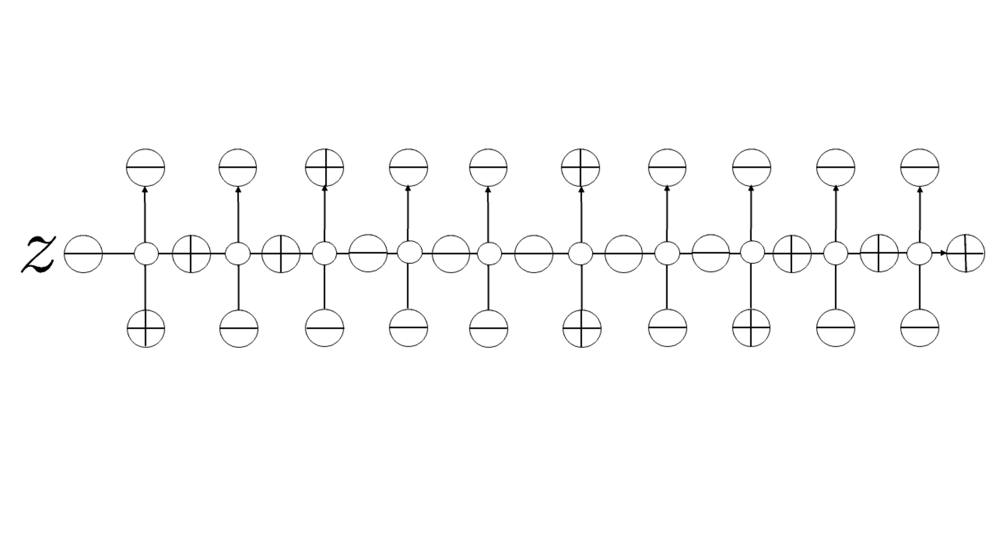
Figure 11: The dual wavefunction ⟨Φ(z1,…,zN)|x1¯⋯xN¯⟩\langle\Phi(z_{1},\dots,z_{N})|\overline{x_{1}}\cdots\overline{x_{N}}\rangle for the case M=5M=5, N=3N=3, (x1¯,x2¯,x3¯)=(1,2,4)(\overline{x_{1}},\overline{x_{2}},\overline{x_{3}})=(1,2,4).

We show the following relation between the dual wavefunction and the symplectic Schur functions.

Theorem 4.1.

The dual wavefunction ⟨Φ(z1,…,zN)|x1¯⋯xN¯⟩\langle\Phi(z_{1},\dots,z_{N})|\overline{x_{1}}\cdots\overline{x_{N}}\rangle can be expressed by the symplectic Schur functions as

⟨Φ(z1,…,zN)|x1¯⋯xN¯⟩\displaystyle\langle\Phi(z_{1},\dots,z_{N})|\overline{x_{1}}\cdots\overline{x_{N}}\rangle
=\displaystyle= tN⁡(M−N)​∏j=1Nzjj−1−N​(1+t​zj2)​∏1≤j<k≤N(1+t​zj​zk)​(1+t​zj​zk−1)​s​pλ¯​({t​z}N).\displaystyle t^{N(M-N)}\prod_{j=1}^{N}z_{j}^{j-1-N}(1+tz_{j}^{2})\prod_{1\leq j<k\leq N}(1+tz_{j}z_{k})(1+tz_{j}z_{k}^{-1})sp_{\overline{\lambda}}(\{tz\}_{N}). (4.3)

Here the Young diagram for the symplectic Schur functions correspond to the hole configuration under the relation λj¯=xN−j+1¯−N+j−1\overline{\lambda_{j}}=\overline{x_{N-j+1}}-N+j-1, j=1,…,Nj=1,\dots,N, and the symmetric variables are {t​z}N={t​z1,…,t​zN}\displaystyle\{tz\}_{N}=\{tz_{1},\dots,tz_{N}\}.

The result of Theorem 4.1 resembles the case for the dual wavefunction without reflecting boundary which gives the Schur polynomials. There is again a factor tN⁡(M−N)t^{N(M-N)} which depends on the number of sites MM and the number of particles NN in the right hand side of (4.3). Also, the symmetric variables of the symplectic Schur functions are {t​z}N\displaystyle\{tz\}_{N}, not simply {z}N\displaystyle\{z\}_{N}.

It seems difficult to directly prove (4.3) itself by using the argument by Ivanov [43], which extends the one for the case without reflecting boundary by Bump-Brubaker-Friedberg [26] to the symplectic ice. As in the case of the paper which we proved the correspondence between the dual wavefunction without reflecting boundary and the Schur polynomials, the key is to transform the statement (4.3) to another equivalent one, which enables us to give a proof by using the argument by Ivanov.

Proof.

We transform (4.3) as follows. First, by rescaling each zjz_{j} to t−1​zjt^{-1}z_{j}, we have

⟨Φ(t−1z1,…,t−1zN)|x1¯⋯xN¯⟩\displaystyle\langle\Phi(t^{-1}z_{1},\dots,t^{-1}z_{N})|\overline{x_{1}}\cdots\overline{x_{N}}\rangle
=\displaystyle= tM​N​∏j=1Nzjj−1−N​(1+t−1​zj2)​∏1≤j<k≤N(1+t−1​zj​zk)​(t−1+zj​zk−1)​s​pλ¯​({z}N).\displaystyle t^{MN}\prod_{j=1}^{N}z_{j}^{j-1-N}(1+t^{-1}z_{j}^{2})\prod_{1\leq j<k\leq N}(1+t^{-1}z_{j}z_{k})(t^{-1}+z_{j}z_{k}^{-1})sp_{\overline{\lambda}}(\{z\}_{N}). (4.4)

We further rewrite (4.4) in the following form.

tN⟨1⋯M|(ℬ⁡(t−1​z1)tM+1)⋯(ℬ⁡(t−1​zN)tM+1)|x1¯⋯xN¯⟩\displaystyle t^{N}\langle 1\cdots M|\Bigg(\frac{\mathcal{B}(t^{-1}z_{1})}{t^{M+1}}\Bigg)\cdots\Bigg(\frac{\mathcal{B}(t^{-1}z_{N})}{t^{M+1}}\Bigg)|\overline{x_{1}}\cdots\overline{x_{N}}\rangle
=\displaystyle= ∏j=1Nzjj−1−N​(1+t−1​zj2)​∏1≤j<k≤N(1+t−1​zj​zk)​(t−1+zj​zk−1)​s​pλ¯​({z}N).\displaystyle\prod_{j=1}^{N}z_{j}^{j-1-N}(1+t^{-1}z_{j}^{2})\prod_{1\leq j<k\leq N}(1+t^{-1}z_{j}z_{k})(t^{-1}+z_{j}z_{k}^{-1})sp_{\overline{\lambda}}(\{z\}_{N}). (4.5)

For giving a proof, it is convenient to introduce the following rescaled LL-operators and KK-matrix

L′​(z,t)=1t​L​(t−1​z,t)=(t−100001t−100(t+1)​z−1z−10000z−1),\displaystyle L^{\prime}(z,t)=\frac{1}{t}L(t^{-1}z,t)=\left(\begin{array}[]{cccc}t^{-1}&0&0&0\\ 0&1&t^{-1}&0\\ 0&(t+1)z^{-1}&z^{-1}&0\\ 0&0&0&z^{-1}\end{array}\right),
L~′​(z,t)=L~​(t−1​z,t)=(t−1​z0000z100(1+t−1)​z100001),\displaystyle\widetilde{L}^{\prime}(z,t)=\widetilde{L}(t^{-1}z,t)=\left(\begin{array}[]{cccc}t^{-1}z&0&0&0\\ 0&z&1&0\\ 0&(1+t^{-1})z&1&0\\ 0&0&0&1\end{array}\right),
K′​(z,t)=1t​K​(t−1​z)=(t−1​z00z−1).\displaystyle K^{\prime}(z,t)=\frac{1}{t}K(t^{-1}z)=\left(\begin{array}[]{cc}t^{-1}z&0\\ 0&z^{-1}\\ \end{array}\right).

We denote the two types of the AA- and BB-operators, the double row BB-operator constructed from these rescaled LL-operators and KK-matrix L′​(z,t)L^{\prime}(z,t), L~′​(z,t)\widetilde{L}^{\prime}(z,t), K′​(z,t)K^{\prime}(z,t) as A′​(z)A^{\prime}(z), B′​(z)B^{\prime}(z), A~′​(z)\widetilde{A}^{\prime}(z), B~′​(z)\widetilde{B}^{\prime}(z) and ℬ′​(z)\mathcal{B}^{\prime}(z) respectively. The double row BB operator is now constructed from the two types of the AA- and BB-operators as

ℬ′​(z)\displaystyle\mathcal{B}^{\prime}(z) =B~′(z)⟨0|K′(z,t)|0⟩aaA′(z)+A~′(z)⟨1|K′(z,t)|1⟩aaB′(z)\displaystyle=\widetilde{B}^{\prime}(z){}_{a}\langle 0|K^{\prime}(z,t)|0\rangle_{a}A^{\prime}(z)+\widetilde{A}^{\prime}(z){}_{a}\langle 1|K^{\prime}(z,t)|1\rangle_{a}B^{\prime}(z) (4.19)
=t−1​z​B~′​(z)​A′​(z)+z−1​A~′​(z)​B′​(z).\displaystyle=t^{-1}z\widetilde{B}^{\prime}(z)A^{\prime}(z)+z^{-1}\widetilde{A}^{\prime}(z)B^{\prime}(z). (4.20)

Using these rescaled objects, (4.5) can be expressed as

tN⟨1⋯M|ℬ′(z1)⋯ℬ′(zN)|x1¯⋯xN¯⟩\displaystyle t^{N}\langle 1\cdots M|\mathcal{B}^{\prime}(z_{1})\cdots\mathcal{B}^{\prime}(z_{N})|\overline{x_{1}}\cdots\overline{x_{N}}\rangle
=\displaystyle= ∏j=1Nzjj−1−N​(1+t−1​zj2)​∏1≤j<k≤N(1+t−1​zj​zk)​(t−1+zj​zk−1)​s​pλ¯​({z}N).\displaystyle\prod_{j=1}^{N}z_{j}^{j-1-N}(1+t^{-1}z_{j}^{2})\prod_{1\leq j<k\leq N}(1+t^{-1}z_{j}z_{k})(t^{-1}+z_{j}z_{k}^{-1})sp_{\overline{\lambda}}(\{z\}_{N}). (4.21)

Instead of proving (4.3), we show (4.21) since this is equivalent to (4.3) and is the expression which one can use the argument given in Ivanov [43].

We first show the following lemma.

Lemma 4.2.
∏j=1NzjN+1−j​(1+t−1​zj2)−1​∏1≤j<k≤N(1+t−1​zj​zk)−1​(t−1+zj​zk−1)−1\displaystyle\prod_{j=1}^{N}z_{j}^{N+1-j}(1+t^{-1}z_{j}^{2})^{-1}\prod_{1\leq j<k\leq N}(1+t^{-1}z_{j}z_{k})^{-1}(t^{-1}+z_{j}z_{k}^{-1})^{-1}
×\displaystyle\times tN⟨1⋯M|ℬ′(z1)⋯ℬ′(zN)|x1¯⋯xN¯⟩\displaystyle t^{N}\langle 1\cdots M|\mathcal{B}^{\prime}(z_{1})\cdots\mathcal{B}^{\prime}(z_{N})|\overline{x_{1}}\cdots\overline{x_{N}}\rangle (4.22)

does not depend on tt.

Proof.

We follow along the lines of the proof by Ivanov [43]. It is enough to prove the following properties for
tN⟨1⋯M|ℬ′(z1)⋯ℬ′(zN)|x1¯⋯xN¯⟩t^{N}\langle 1\cdots M|\mathcal{B}^{\prime}(z_{1})\cdots\mathcal{B}^{\prime}(z_{N})|\overline{x_{1}}\cdots\overline{x_{N}}\rangle:

  1. 1.

    tN⟨1⋯M|ℬ′(z1)⋯ℬ′(zN)|x1¯⋯xN¯⟩t^{N}\langle 1\cdots M|\mathcal{B}^{\prime}(z_{1})\cdots\mathcal{B}^{\prime}(z_{N})|\overline{x_{1}}\cdots\overline{x_{N}}\rangle is a polynomial of t′:=t−1t^{\prime}:=t^{-1} with its highest degree at most N2N^{2}.

  2. 2.

    tN⟨1⋯M|ℬ′(z1)⋯ℬ′(zN)|x1¯⋯xN¯⟩/D′t^{N}\langle 1\cdots M|\mathcal{B}^{\prime}(z_{1})\cdots\mathcal{B}^{\prime}(z_{N})|\overline{x_{1}}\cdots\overline{x_{N}}\rangle/D^{\prime},
    where D′:=∏j=1Nzjj−1−N​(1+t′​zj2)​∏1≤j<k≤N(1+t′​zj​zk)​(t′+zj​zk−1)D^{\prime}:=\prod_{j=1}^{N}z_{j}^{j-1-N}(1+t^{\prime}z_{j}^{2})\prod_{1\leq j<k\leq N}(1+t^{\prime}z_{j}z_{k})(t^{\prime}+z_{j}z_{k}^{-1}), is invariant under any permutation of z1,…,zNz_{1},\dots,z_{N}.

  3. 3.

    tN⟨1⋯M|ℬ′(z1)⋯ℬ′(zN)|x1¯⋯xN¯⟩/D′t^{N}\langle 1\cdots M|\mathcal{B}^{\prime}(z_{1})\cdots\mathcal{B}^{\prime}(z_{N})|\overline{x_{1}}\cdots\overline{x_{N}}\rangle/D^{\prime} is invariant under zi⟷zi−1z_{i}\longleftrightarrow z_{i}^{-1}.

We first show degt′(tN⟨1⋯M|ℬ′(z1)⋯ℬ′(zN)|x1¯⋯xN¯⟩)≤N2\mathrm{deg}_{t^{\prime}}(t^{N}\langle 1\cdots M|\mathcal{B}^{\prime}(z_{1})\cdots\mathcal{B}^{\prime}(z_{N})|\overline{x_{1}}\cdots\overline{x_{N}}\rangle)\leq N^{2} by induction on NN. We use the following properties for the matrix elements of the AA- and BB-operators, which can easily be seen from the matrix elements of the LL-operators.

0≤degt′(t⟨x1¯⋯xN¯|A′(z)|y1¯⋯yN¯⟩)≤N−1,N≥1,\displaystyle 0\leq\mathrm{deg}_{t^{\prime}}(t\langle\overline{x_{1}}\cdots\overline{x_{N}}|A^{\prime}(z)|\overline{y_{1}}\cdots\overline{y_{N}}\rangle)\leq N-1,\ \ \ N\geq 1, (4.23)
0≤degt′(t⟨x1¯⋯xN¯|B′(z)|y1¯⋯yN+1¯⟩)≤N,N≥0,\displaystyle 0\leq\mathrm{deg}_{t^{\prime}}(t\langle\overline{x_{1}}\cdots\overline{x_{N}}|B^{\prime}(z)|\overline{y_{1}}\cdots\overline{y_{N+1}}\rangle)\leq N,\ \ \ N\geq 0, (4.24)
0≤degt′(⟨x1¯⋯xN¯|A~′(z)|y1¯⋯yN¯⟩)≤N,N≥0,\displaystyle 0\leq\mathrm{deg}_{t^{\prime}}(\langle\overline{x_{1}}\cdots\overline{x_{N}}|\widetilde{A}^{\prime}(z)|\overline{y_{1}}\cdots\overline{y_{N}}\rangle)\leq N,\ \ \ N\geq 0, (4.25)
0≤degt′(⟨x1¯⋯xN¯|B~′(z)|y1¯⋯yN+1¯⟩)≤N,N≥0.\displaystyle 0\leq\mathrm{deg}_{t^{\prime}}(\langle\overline{x_{1}}\cdots\overline{x_{N}}|\widetilde{B}^{\prime}(z)|\overline{y_{1}}\cdots\overline{y_{N+1}}\rangle)\leq N,\ \ \ N\geq 0. (4.26)

We first remark that it is enough to consider the above matrix elements, since all of the non-zero matrix elements are included in the above cases. For example, one does not need to consider ⟨x1¯⋯xN¯|A′(z)|y1¯⋯yN+1¯⟩\langle\overline{x_{1}}\cdots\overline{x_{N}}|A^{\prime}(z)|\overline{y_{1}}\cdots\overline{y_{N+1}}\rangle. This is because due to the so-called ice rule ⟨δ|⟨γ|L(z)|α⟩aj|β⟩ja=0{}_{a}\langle\delta|{}_{j}\langle\gamma|L(z)|\alpha\rangle_{a}|\beta\rangle_{j}=0 unless α+β=γ+δ\alpha+\beta=\gamma+\delta for the LL-operator of the six-vertex model, the AA-operators preserve the total number of holes in the quantum space, hence
⟨x1¯⋯xN¯|A′(z)|y1¯⋯yN+1¯⟩=0\langle\overline{x_{1}}\cdots\overline{x_{N}}|A^{\prime}(z)|\overline{y_{1}}\cdots\overline{y_{N+1}}\rangle=0 follows immediately. Similary, the BB-operators increase the total number of holes in the quantum space by one, one can see ⟨x1¯⋯xN¯|B′(z)|y1¯⋯yN¯⟩=0\langle\overline{x_{1}}\cdots\overline{x_{N}}|B^{\prime}(z)|\overline{y_{1}}\cdots\overline{y_{N}}\rangle=0 immediately. It is not difficult to find the above properties of the degree with respect to t′t^{\prime} by taking the ice-rule into account.

Let us show Property 1 for the case N=1N=1. We use the decomposition of the double row BB-operator (4.20) and insert the completeness relation ∑y¯|y¯⟩​⟨y¯|=Id\displaystyle\sum_{\overline{y}}|\overline{y}\rangle\langle\overline{y}|=\mathrm{Id} between the AA- and BB-operators to deform dett′(t⟨1⋯M|ℬ′(z)|x¯⟩)\mathrm{det}_{t^{\prime}}(t\langle 1\cdots M|\mathcal{B}^{\prime}(z)|\overline{x}\rangle) as

dett′(t⟨1⋯M|ℬ′(z)|x¯⟩)=dett′(t⟨1⋯M|(t−1zB~′(z)A′(z)+z−1A~′(z)B′(z))|x¯⟩)\displaystyle\mathrm{det}_{t^{\prime}}(t\langle 1\cdots M|\mathcal{B}^{\prime}(z)|\overline{x}\rangle)=\mathrm{det}_{t^{\prime}}(t\langle 1\cdots M|(t^{-1}z\widetilde{B}^{\prime}(z)A^{\prime}(z)+z^{-1}\widetilde{A}^{\prime}(z)B^{\prime}(z))|\overline{x}\rangle)
=\displaystyle= degt′(t−1z∑y¯⟨1⋯M|B~′(z)|y¯⟩⟨y¯|tA′(z)|x¯⟩+z−1⟨1⋯M|A~′(z)|1⋯M⟩⟨1⋯M|tB′(z)|x¯⟩).\displaystyle\mathrm{deg}_{t^{\prime}}(t^{-1}z\sum_{\overline{y}}\langle 1\cdots M|\widetilde{B}^{\prime}(z)|\overline{y}\rangle\langle\overline{y}|tA^{\prime}(z)|\overline{x}\rangle+z^{-1}\langle 1\cdots M|\widetilde{A}^{\prime}(z)|1\cdots M\rangle\langle 1\cdots M|tB^{\prime}(z)|\overline{x}\rangle). (4.27)

Using the generic property of the degree deg⁡(P+Q)=Max⁡(deg​P,deg​Q)\mathrm{deg}(P+Q)=\mathrm{Max}(\mathrm{deg}P,\mathrm{deg}Q) and the properties (4.23), (4.24), (4.25) and (4.26), it follows that 0≤degt′(t⟨1⋯M|ℬ′(z)|x¯⟩)≤10\leq\mathrm{deg}_{t^{\prime}}(t\langle 1\cdots M|\mathcal{B}^{\prime}(z)|\overline{x}\rangle)\leq 1.

Next, let us assume degt′(tN⟨1⋯M|ℬ′(z1)⋯ℬ′(zN)|x1¯⋯xN¯⟩)≤N2\mathrm{deg}_{t^{\prime}}(t^{N}\langle 1\cdots M|\mathcal{B}^{\prime}(z_{1})\cdots\mathcal{B}^{\prime}(z_{N})|\overline{x_{1}}\cdots\overline{x_{N}}\rangle)\leq N^{2}. Let us show 0≤degt′(t⟨x1¯⋯xN¯|ℬ′(z)|y1¯⋯yN+1¯⟩)≤2N+10\leq\mathrm{deg}_{t^{\prime}}(t\langle\overline{x_{1}}\cdots\overline{x_{N}}|\mathcal{B}^{\prime}(z)|\overline{y_{1}}\cdots\overline{y_{N+1}}\rangle)\leq 2N+1. This can be seen as above by using the decomposition of the double row BB-operator (4.20) and inserting the completeness relation to deform degt′(t⟨x1¯⋯xN¯|ℬ′(z)|y1¯⋯yN+1¯⟩)\mathrm{deg}_{t^{\prime}}(t\langle\overline{x_{1}}\cdots\overline{x_{N}}|\mathcal{B}^{\prime}(z)|\overline{y_{1}}\cdots\overline{y_{N+1}}\rangle) as

degt′(t⟨x1¯⋯xN¯|ℬ′(z)|y1¯⋯yN+1¯⟩)\displaystyle\mathrm{deg}_{t^{\prime}}(t\langle\overline{x_{1}}\cdots\overline{x_{N}}|\mathcal{B}^{\prime}(z)|\overline{y_{1}}\cdots\overline{y_{N+1}}\rangle)
=\displaystyle= degt′(t⟨x1¯⋯xN¯|(t−1zB~′(z)A′(z)+z−1A~′(z)B′(z))|y1¯⋯yN+1¯⟩)\displaystyle\mathrm{deg}_{t^{\prime}}(t\langle\overline{x_{1}}\cdots\overline{x_{N}}|(t^{-1}z\widetilde{B}^{\prime}(z)A^{\prime}(z)+z^{-1}\widetilde{A}^{\prime}(z)B^{\prime}(z))|\overline{y_{1}}\cdots\overline{y_{N+1}}\rangle)
=\displaystyle= degt′(t−1z∑{u¯}⟨x1¯⋯xN¯|B~′(z)|u1¯⋯uN+1¯⟩⟨u1¯⋯uN+1¯|tA′(z)|y1¯⋯yN+1¯⟩\displaystyle\mathrm{deg}_{t^{\prime}}\Bigg(t^{-1}z\sum_{\{\overline{u}\}}\langle\overline{x_{1}}\cdots\overline{x_{N}}|\widetilde{B}^{\prime}(z)|\overline{u_{1}}\cdots\overline{u_{N+1}}\rangle\langle\overline{u_{1}}\cdots\overline{u_{N+1}}|tA^{\prime}(z)|\overline{y_{1}}\cdots\overline{y_{N+1}}\rangle
+\displaystyle+ z−1∑{v¯}⟨x1¯⋯xN¯|A~′(z)|v1¯⋯vN¯⟩⟨v1¯⋯vN¯|tB′(z)|y1¯⋯yN+1¯⟩),\displaystyle z^{-1}\sum_{\{\overline{v}\}}\langle\overline{x_{1}}\cdots\overline{x_{N}}|\widetilde{A}^{\prime}(z)|\overline{v_{1}}\cdots\overline{v_{N}}\rangle\langle\overline{v_{1}}\cdots\overline{v_{N}}|tB^{\prime}(z)|\overline{y_{1}}\cdots\overline{y_{N+1}}\rangle\Bigg), (4.28)

and using deg⁡(P+Q)=Max⁡(deg​P,deg​Q)\mathrm{deg}(P+Q)=\mathrm{Max}(\mathrm{deg}P,\mathrm{deg}Q), the properties (4.23), (4.24), (4.25) and (4.26).

One can finally see degt′(tN+1⟨1⋯M|ℬ′(z1)⋯ℬ′(zN+1)|y1¯⋯yN+1¯⟩)≤(N+1)2\mathrm{deg}_{t^{\prime}}(t^{N+1}\langle 1\cdots M|\mathcal{B}^{\prime}(z_{1})\cdots\mathcal{B}^{\prime}(z_{N+1})|\overline{y_{1}}\cdots\overline{y_{N+1}}\rangle)\leq(N+1)^{2} by using the property 0≤degt′(t⟨x1¯⋯xN¯|ℬ′(z)|y1¯⋯yN+1¯⟩)≤2N+10\leq\mathrm{deg}_{t^{\prime}}(t\langle\overline{x_{1}}\cdots\overline{x_{N}}|\mathcal{B}^{\prime}(z)|\overline{y_{1}}\cdots\overline{y_{N+1}}\rangle)\leq 2N+1 together with the assumption degt′(tN⟨1⋯M|ℬ′(z1)⋯ℬ′(zN)|x1¯⋯xN¯⟩)≤N2\mathrm{deg}_{t^{\prime}}(t^{N}\langle 1\cdots M|\mathcal{B}^{\prime}(z_{1})\cdots\mathcal{B}^{\prime}(z_{N})|\overline{x_{1}}\cdots\overline{x_{N}}\rangle)\leq N^{2} and the decomposition

tN+1⟨1⋯M|ℬ′(z1)⋯ℬ′(zN+1)|y1¯⋯yN+1¯⟩\displaystyle t^{N+1}\langle 1\cdots M|\mathcal{B}^{\prime}(z_{1})\cdots\mathcal{B}^{\prime}(z_{N+1})|\overline{y_{1}}\cdots\overline{y_{N+1}}\rangle
=\displaystyle= ∑{x¯}(tN⟨1⋯M|ℬ′(z1)⋯ℬ′(zN)|x1¯⋯xN¯⟩)(t⟨x1¯⋯xN¯|ℬ′(zN+1)|y1¯⋯yN+1¯⟩).\displaystyle\sum_{\{\overline{x}\}}(t^{N}\langle 1\cdots M|\mathcal{B}^{\prime}(z_{1})\cdots\mathcal{B}^{\prime}(z_{N})|\overline{x_{1}}\cdots\overline{x_{N}}\rangle)(t\langle\overline{x_{1}}\cdots\overline{x_{N}}|\mathcal{B}^{\prime}(z_{N+1})|\overline{y_{1}}\cdots\overline{y_{N+1}}\rangle). (4.29)

Property 2 can be proved exactly in the same way as in Lemma 2 in Ivanov [43] which is a lengthy one, since one needs many local relations and arguments to prove the lemma. Instead, given below is a shortcut of the argument by transforming his result to Property 2. First, one notes that Ivanov’s proof of Lemma 2 shows that not only ⟨x1⋯xN|ℬ(z1)⋯ℬ(zN)|Ω⟩\langle x_{1}\cdots x_{N}|\mathcal{B}(z_{1})\cdots\mathcal{B}(z_{N})|\Omega\rangle but also every matrix element ⟨y1⋯yn+N|ℬ(z1)⋯ℬ(zN)|x1⋯xn⟩\langle y_{1}\cdots y_{n+N}|\mathcal{B}(z_{1})\cdots\mathcal{B}(z_{N})|x_{1}\cdots x_{n}\rangle has the property that ⟨y1⋯yn+N|ℬ(z1)⋯ℬ(zN)|x1⋯xn⟩/D\langle y_{1}\cdots y_{n+N}|\mathcal{B}(z_{1})\cdots\mathcal{B}(z_{N})|x_{1}\cdots x_{n}\rangle/D where D:=∏j=1Nzjj−1−N​(1+t​zj2)​∏1≤j<k≤N(1+t​zj​zk)​(1+t​zj​zk−1)D:=\prod_{j=1}^{N}z_{j}^{j-1-N}(1+tz_{j}^{2})\prod_{1\leq j<k\leq N}(1+tz_{j}z_{k})(1+tz_{j}z_{k}^{-1}), is invariant under any permutation zi⟷zjz_{i}\longleftrightarrow z_{j}.

From the fact that the rescaled double row BB-operator ℬ′​(z)\mathcal{B}^{\prime}(z) consists of rescaled LL-operators and KK-matrix, which can be essentially obtained from the original LL-operators and KK-matrix by the changing the spectral parameters z⟶t−1​zz\longrightarrow t^{-1}z, the statement of the invariance for the matrix element ⟨y1⋯yn+N|ℬ(z1)⋯ℬ(zN)|x1⋯xn⟩\langle y_{1}\cdots y_{n+N}|\mathcal{B}(z_{1})\cdots\mathcal{B}(z_{N})|x_{1}\cdots x_{n}\rangle can be converted to the statement that every matrix element ⟨x1¯⋯xn¯|ℬ′(z1)⋯ℬ′(zN)|y1¯⋯yn+N¯⟩\langle\overline{x_{1}}\cdots\overline{x_{n}}|\mathcal{B}^{\prime}(z_{1})\cdots\mathcal{B}^{\prime}(z_{N})|\overline{y_{1}}\cdots\overline{y_{n+N}}\rangle has the property that tN⟨x1¯⋯xn¯|ℬ′(z1)⋯ℬ′(zN)|y1¯⋯yn+N¯⟩/D′t^{N}\langle\overline{x_{1}}\cdots\overline{x_{n}}|\mathcal{B}^{\prime}(z_{1})\cdots\mathcal{B}^{\prime}(z_{N})|\overline{y_{1}}\cdots\overline{y_{n+N}}\rangle/D^{\prime} where D′=∏j=1Nzjj−1−N​(1+t′​zj2)​∏1≤j<k≤N(1+t′​zj​zk)​(t′+zj​zk−1)D^{\prime}=\prod_{j=1}^{N}z_{j}^{j-1-N}(1+t^{\prime}z_{j}^{2})\prod_{1\leq j<k\leq N}(1+t^{\prime}z_{j}z_{k})(t^{\prime}+z_{j}z_{k}^{-1}), t′=t−1t^{\prime}=t^{-1}, is invariant under any permutation zi⟷zjz_{i}\longleftrightarrow z_{j}. Property 2 follows from this statement since we are considering a special matrix element tN⟨1⋯M|ℬ′(z1)⋯ℬ′(zN)|x1¯⋯xN¯⟩/D′t^{N}\langle 1\cdots M|\mathcal{B}^{\prime}(z_{1})\cdots\mathcal{B}^{\prime}(z_{N})|\overline{x_{1}}\cdots\overline{x_{N}}\rangle/D^{\prime}.

We prove Property 3 as follows. Since one cannot apply Ivanov’s argument as exactly as it is due to the change of the matrix elements of the LL-operators, we modify the argument as follows. First, we find that it is enough to show

⟨1⋯M|ℬ′(z)|x¯⟩=(1+t−1​z2)t​zzλ¯+1−z−λ¯−1z−z−1,λ¯=x¯−1.\displaystyle\langle 1\cdots M|\mathcal{B}^{\prime}(z)|\overline{x}\rangle=\frac{(1+t^{-1}z^{2})}{tz}\frac{z^{\overline{\lambda}+1}-z^{-\overline{\lambda}-1}}{z-z^{-1}},\ \ \ \overline{\lambda}=\overline{x}-1. (4.30)

From (4.30) and using the decomposition,

⟨1⋯M|ℬ′(z1)⋯ℬ′(zN)|x1¯⋯xN¯⟩=∑y¯⟨1⋯M|ℬ′(z1)|y¯⟩⟨y¯|ℬ′(z2)⋯ℬ′(zN)|x1¯⋯xN¯⟩,\displaystyle\langle 1\cdots M|\mathcal{B}^{\prime}(z_{1})\cdots\mathcal{B}^{\prime}(z_{N})|\overline{x_{1}}\cdots\overline{x_{N}}\rangle=\sum_{\overline{y}}\langle 1\cdots M|\mathcal{B}^{\prime}(z_{1})|\overline{y}\rangle\langle\overline{y}|\mathcal{B}^{\prime}(z_{2})\cdots\mathcal{B}^{\prime}(z_{N})|\overline{x_{1}}\cdots\overline{x_{N}}\rangle, (4.31)

we have

⟨1⋯M|ℬ′(z1)⋯ℬ′(zN)|x1¯⋯xN¯⟩=(1+t−1​z12)t​z1∑y¯z1y¯−z1−y¯z1−z1−1⟨y¯|ℬ′(z2)⋯ℬ′(zN)|x1¯⋯xN¯⟩,\displaystyle\langle 1\cdots M|\mathcal{B}^{\prime}(z_{1})\cdots\mathcal{B}^{\prime}(z_{N})|\overline{x_{1}}\cdots\overline{x_{N}}\rangle=\frac{(1+t^{-1}z_{1}^{2})}{tz_{1}}\sum_{\overline{y}}\frac{z_{1}^{\overline{y}}-z_{1}^{-\overline{y}}}{z_{1}-z_{1}^{-1}}\langle\overline{y}|\mathcal{B}^{\prime}(z_{2})\cdots\mathcal{B}^{\prime}(z_{N})|\overline{x_{1}}\cdots\overline{x_{N}}\rangle, (4.32)

from which one gets

tN⟨1⋯M|ℬ′(z1)⋯ℬ′(zN)|x1¯⋯xN¯⟩tN⟨1⋯M|ℬ′(z1)⋯ℬ′(zN)|x1¯⋯xN¯⟩|z1⟷z1−1=(t′​z1+z1−1)(z1+t′​z1−1).\displaystyle\frac{t^{N}\langle 1\cdots M|\mathcal{B}^{\prime}(z_{1})\cdots\mathcal{B}^{\prime}(z_{N})|\overline{x_{1}}\cdots\overline{x_{N}}\rangle}{t^{N}\langle 1\cdots M|\mathcal{B}^{\prime}(z_{1})\cdots\mathcal{B}^{\prime}(z_{N})|\overline{x_{1}}\cdots\overline{x_{N}}\rangle|_{z_{1}\longleftrightarrow z_{1}^{-1}}}=\frac{(t^{\prime}z_{1}+z_{1}^{-1})}{(z_{1}+t^{\prime}z_{1}^{-1})}. (4.33)

This ratio and D′D′|z1⟷z1−1=(t′​z1+z1−1)(z1+t′​z1−1)\displaystyle\frac{D^{\prime}}{D^{\prime}|_{z_{1}\longleftrightarrow z_{1}^{-1}}}=\frac{(t^{\prime}z_{1}+z_{1}^{-1})}{(z_{1}+t^{\prime}z_{1}^{-1})} gives the relation

tN⟨1⋯M|ℬ′(z1)⋯ℬ′(zN)|x1¯⋯xN¯⟩/D′\displaystyle t^{N}\langle 1\cdots M|\mathcal{B}^{\prime}(z_{1})\cdots\mathcal{B}^{\prime}(z_{N})|\overline{x_{1}}\cdots\overline{x_{N}}\rangle/D^{\prime}
=\displaystyle= tN⟨1⋯M|ℬ′(z1)⋯ℬ′(zN)|x1¯⋯xN¯⟩/D′|z1⟷z1−1,\displaystyle t^{N}\langle 1\cdots M|\mathcal{B}^{\prime}(z_{1})\cdots\mathcal{B}^{\prime}(z_{N})|\overline{x_{1}}\cdots\overline{x_{N}}\rangle/D^{\prime}\Big|_{z_{1}\longleftrightarrow z_{1}^{-1}}, (4.34)

which shows that tN⟨1⋯M|ℬ′(z1)⋯ℬ′(zN)|x1¯⋯xN¯⟩/D′t^{N}\langle 1\cdots M|\mathcal{B}^{\prime}(z_{1})\cdots\mathcal{B}^{\prime}(z_{N})|\overline{x_{1}}\cdots\overline{x_{N}}\rangle/D^{\prime} is invariant under z1⟷z1−1z_{1}\longleftrightarrow z_{1}^{-1}. Together with Property 2, one gets Property 3.

Let us show (4.30). We insert the completeness relation to decompose ⟨1⋯M|ℬ′(z)|x¯⟩\langle 1\cdots M|\mathcal{B}^{\prime}(z)|\overline{x}\rangle as

⟨1⋯M|ℬ′(z)|x¯⟩\displaystyle\langle 1\cdots M|\mathcal{B}^{\prime}(z)|\overline{x}\rangle
=\displaystyle= t−1z∑y¯⟨1⋯M|B~′(z)|y¯⟩⟨y¯|A′(z)|x¯⟩+z−1⟨1⋯M|A~′(z)|1⋯M⟩⟨1⋯M|B′(z)|x¯⟩\displaystyle t^{-1}z\sum_{\overline{y}}\langle 1\cdots M|\widetilde{B}^{\prime}(z)|\overline{y}\rangle\langle\overline{y}|A^{\prime}(z)|\overline{x}\rangle+z^{-1}\langle 1\cdots M|\widetilde{A}^{\prime}(z)|1\cdots M\rangle\langle 1\cdots M|B^{\prime}(z)|\overline{x}\rangle
=\displaystyle= t−1z∑y¯=1,…,x¯−1⟨1⋯M|B~′(z)|y¯⟩⟨y¯|A′(z)|x¯⟩\displaystyle t^{-1}z\sum_{\overline{y}=1,\dots,\overline{x}-1}\langle 1\cdots M|\widetilde{B}^{\prime}(z)|\overline{y}\rangle\langle\overline{y}|A^{\prime}(z)|\overline{x}\rangle
+t−1z⟨1⋯M|B~′(z)|x¯⟩⟨x¯|A′(z)|x¯⟩+z−1⟨1⋯M|A~′(z)|1⋯M⟩⟨1⋯M|B′(z)|x¯⟩.\displaystyle+t^{-1}z\langle 1\cdots M|\widetilde{B}^{\prime}(z)|\overline{x}\rangle\langle\overline{x}|A^{\prime}(z)|\overline{x}\rangle+z^{-1}\langle 1\cdots M|\widetilde{A}^{\prime}(z)|1\cdots M\rangle\langle 1\cdots M|B^{\prime}(z)|\overline{x}\rangle. (4.35)

Inserting the explicit forms of the matrix elements

⟨1⋯M|B~′(z)|y¯⟩\displaystyle\langle 1\cdots M|\widetilde{B}^{\prime}(z)|\overline{y}\rangle =zy¯−1,y¯=1,…,x¯−1,\displaystyle=z^{\overline{y}-1},\ \ \ \overline{y}=1,\dots,\overline{x}-1, (4.36)
⟨y¯|A′​(z)|x¯⟩\displaystyle\langle\overline{y}|A^{\prime}(z)|\overline{x}\rangle =t+1tz−x¯+y¯,y¯=1,…,x¯−1,\displaystyle=\frac{t+1}{t}z^{-\overline{x}+\overline{y}},\ \ \ \overline{y}=1,\dots,\overline{x}-1, (4.37)
⟨1⋯M|B~′(z)|x¯⟩\displaystyle\langle 1\cdots M|\widetilde{B}^{\prime}(z)|\overline{x}\rangle =zx¯−1,\displaystyle=z^{\overline{x}-1}, (4.38)
⟨x¯|A′​(z)|x¯⟩\displaystyle\langle\overline{x}|A^{\prime}(z)|\overline{x}\rangle =1t,\displaystyle=\frac{1}{t}, (4.39)
⟨1⋯M|A~′(z)|1⋯M⟩\displaystyle\langle 1\cdots M|\widetilde{A}^{\prime}(z)|1\cdots M\rangle =1,\displaystyle=1, (4.40)
⟨1⋯M|B′(z)|x¯⟩\displaystyle\langle 1\cdots M|B^{\prime}(z)|\overline{x}\rangle =1t​z−x¯+1,\displaystyle=\frac{1}{t}z^{-\overline{x}+1}, (4.41)

into the right hand side of (4.35), we have

⟨1⋯M|ℬ′(z)|x¯⟩=\displaystyle\langle 1\cdots M|\mathcal{B}^{\prime}(z)|\overline{x}\rangle= t−1​z​∑y¯=1,…,x¯−1t+1t​z−x¯+y¯​zy¯−1+t−1​z​1t​zx¯−1+z−1​1t​z−x¯+1\displaystyle t^{-1}z\sum_{\overline{y}=1,\dots,\overline{x}-1}\frac{t+1}{t}z^{-\overline{x}+\overline{y}}z^{\overline{y}-1}+t^{-1}z\frac{1}{t}z^{\overline{x}-1}+z^{-1}\frac{1}{t}z^{-\overline{x}+1}
=\displaystyle= t−2​(t+1)​zx¯−1−z1−x¯z−z−1+t−2​zx¯+t−1​z−x¯\displaystyle t^{-2}(t+1)\frac{z^{\overline{x}-1}-z^{1-\overline{x}}}{z-z^{-1}}+t^{-2}z^{\overline{x}}+t^{-1}z^{-\overline{x}}
=\displaystyle= z+t​z−1t2​(z−z−1)​(zx¯−z−x¯)=(1+t−1​z2)t​z​zλ¯+1−z−λ¯−1z−z−1,\displaystyle\frac{z+tz^{-1}}{t^{2}(z-z^{-1})}(z^{\overline{x}}-z^{-\overline{x}})=\frac{(1+t^{-1}z^{2})}{tz}\frac{z^{\overline{\lambda}+1}-z^{-\overline{\lambda}-1}}{z-z^{-1}}, (4.42)

and (4.30) is shown.

Properties 1, 2 and 3 show that tN⟨1⋯M|ℬ′(z1)⋯ℬ′(zN)|x1¯⋯xN¯⟩t^{N}\langle 1\cdots M|\mathcal{B}^{\prime}(z_{1})\cdots\mathcal{B}^{\prime}(z_{N})|\overline{x_{1}}\cdots\overline{x_{N}}\rangle is a polynomial of t′t^{\prime} with highest degree 2​N22N^{2}, and is divided by D′=∏j=1Nzjj−1−N​(1+t′​zj2)​∏1≤j<k≤N(1+t′​zj​zk)​(t′+zj​zk−1)D^{\prime}=\prod_{j=1}^{N}z_{j}^{j-1-N}(1+t^{\prime}z_{j}^{2})\prod_{1\leq j<k\leq N}(1+t^{\prime}z_{j}z_{k})(t^{\prime}+z_{j}z_{k}^{-1}). Hence, Lemma 4.2 is proved.

∎

From Lemma 4.2, one sees that to study the wavefunction, it is enough to examine a particular value of tt. At the point t=−1t=-1, the six-vertex model reduces to a five-vertex model since the first LL-operator becomes

L′​(z,−1)=−L⁡(−z,−1)=(−100001−1000z−10000z−1),\displaystyle L^{\prime}(z,-1)=-L(-z,-1)=\left(\begin{array}[]{cccc}-1&0&0&0\\ 0&1&-1&0\\ 0&0&z^{-1}&0\\ 0&0&0&z^{-1}\end{array}\right),

and second LL-operator becomes

L~′​(z,−1)=L~​(−z,−1)=(−z0000z1000100001).\displaystyle\widetilde{L}^{\prime}(z,-1)=\widetilde{L}(-z,-1)=\left(\begin{array}[]{cccc}-z&0&0&0\\ 0&z&1&0\\ 0&0&1&0\\ 0&0&0&1\end{array}\right).

The KK-matrix at t=−1t=-1 becomes

K′​(z,−1)=−K⁡(−z,−1)=(t​z00z−1).\displaystyle K^{\prime}(z,-1)=-K(-z,-1)=\left(\begin{array}[]{cc}tz&0\\ 0&z^{-1}\\ \end{array}\right).

It is easy to examine at this reduced point t=−1t=-1, and we find the following relation.

Lemma 4.3.

We have

∏j=1NzjN+1−j​(1+t−1​zj2)−1​∏1≤j<k≤N(1+t−1​zj​zk)−1​(t−1+zj​zk−1)−1\displaystyle\prod_{j=1}^{N}z_{j}^{N+1-j}(1+t^{-1}z_{j}^{2})^{-1}\prod_{1\leq j<k\leq N}(1+t^{-1}z_{j}z_{k})^{-1}(t^{-1}+z_{j}z_{k}^{-1})^{-1}
×\displaystyle\times tN⟨1⋯M|ℬ′(z1)⋯ℬ′(zN)|x1¯⋯xN¯⟩|t=−1=spλ¯({z}N).\displaystyle t^{N}\langle 1\cdots M|\mathcal{B}^{\prime}(z_{1})\cdots\mathcal{B}^{\prime}(z_{N})|\overline{x_{1}}\cdots\overline{x_{N}}\rangle\Bigg|_{t=-1}=sp_{\overline{\lambda}}(\{z\}_{N}). (4.56)
Proof.

From the factorization formula of the determinant

detN​(zjN−k+1−zj−N+k−1)=(−1)N​∏j=1Nzjj−1−N​(1−zj2)​∏1≤j<k≤N(1−zj​zk)​(1−zj​zk−1),\displaystyle\mathrm{det}_{N}(z_{j}^{N-k+1}-z_{j}^{-N+k-1})=(-1)^{N}\prod_{j=1}^{N}z_{j}^{j-1-N}(1-z_{j}^{2})\prod_{1\leq j<k\leq N}(1-z_{j}z_{k})(1-z_{j}z_{k}^{-1}), (4.57)

and the definition of the symplectic Schur functions (3.1), one sees that proving the Lemma is equivalent to showing the following equality

⟨1⋯M|ℬ′(z1)⋯ℬ′(zN)|x1¯⋯xN¯⟩=(−1)N⁡(N−1)/2detN(zjλk+N−k+1−zj−λk−N+k−1).\displaystyle\langle 1\cdots M|\mathcal{B}^{\prime}(z_{1})\cdots\mathcal{B}^{\prime}(z_{N})|\overline{x_{1}}\cdots\overline{x_{N}}\rangle=(-1)^{N(N-1)/2}\mathrm{det}_{N}(z_{j}^{\lambda_{k}+N-k+1}-z_{j}^{-\lambda_{k}-N+k-1}). (4.58)

To show this, let us first list the matrix elements of the single AA- and BB-operators.

Lemma 4.4.

We have the following explicit expressions for the matrix elements of the AA- and BB-operators at t=−1t=-1.
(1) The matrix element of A′​(z)A^{\prime}(z) is given by

⟨x1¯⋯xk¯|A′(z)|y1¯⋯yk¯⟩=\displaystyle\langle\overline{x_{1}}\cdots\overline{x_{k}}|A^{\prime}(z)|\overline{y_{1}}\cdots\overline{y_{k}}\rangle= (−1)k​∏j=1kδxj¯​yj¯.\displaystyle(-1)^{k}\prod_{j=1}^{k}\delta_{\overline{x_{j}}\overline{y_{j}}}. (4.59)

(2) The matrix element of B′​(z)B^{\prime}(z) is given by

⟨x1¯⋯xk−1¯|B′(z)|y1¯⋯yk¯⟩=\displaystyle\langle\overline{x_{1}}\cdots\overline{x_{k-1}}|B^{\prime}(z)|\overline{y_{1}}\cdots\overline{y_{k}}\rangle= (−1)k​(−1)j−1​z1−yj¯,\displaystyle(-1)^{k}(-1)^{j-1}z^{1-\overline{y_{j}}}, (4.60)

when the hole configurations {x¯}\{\overline{x}\} and {y¯}\{\overline{y}\} satisfy
x1¯=y1¯,⋯,xj−1¯=yj−1¯\overline{x_{1}}=\overline{y_{1}},\cdots,\overline{x_{j-1}}=\overline{y_{j-1}}, xj¯=yj+1¯,⋯,xk−1¯=yk¯\overline{x_{j}}=\overline{y_{j+1}},\cdots,\overline{x_{k-1}}=\overline{y_{k}} for some jj, and 0 otherwise.

(3) The matrix element of A~′​(z)\widetilde{A}^{\prime}(z) is given by

⟨x1¯⋯xk¯|A~′(z)|y1¯⋯yk¯⟩=\displaystyle\langle\overline{x_{1}}\cdots\overline{x_{k}}|\widetilde{A}^{\prime}(z)|\overline{y_{1}}\cdots\overline{y_{k}}\rangle= ∏j=1kδxj¯​yj¯,\displaystyle\prod_{j=1}^{k}\delta_{\overline{x_{j}}\overline{y_{j}}}, (4.61)

(4) The matrix element of B~′​(z)\widetilde{B}^{\prime}(z) is given by

⟨x1¯⋯xk−1¯|B~′(z)|y1¯⋯yk¯⟩=\displaystyle\langle\overline{x_{1}}\cdots\overline{x_{k-1}}|\widetilde{B}^{\prime}(z)|\overline{y_{1}}\cdots\overline{y_{k}}\rangle= (−1)j−1​zyj¯−1,\displaystyle(-1)^{j-1}z^{\overline{y_{j}}-1}, (4.62)

when the hole configurations {x¯}\{\overline{x}\} and {y¯}\{\overline{y}\} satisfy
x1¯=y1¯,⋯,xj−1¯=yj−1¯\overline{x_{1}}=\overline{y_{1}},\cdots,\overline{x_{j-1}}=\overline{y_{j-1}}, xj¯=yj+1¯,⋯,xk−1¯=yk¯\overline{x_{j}}=\overline{y_{j+1}},\cdots,\overline{x_{k-1}}=\overline{y_{k}} for some jj, and 0 otherwise.

Using these explicit forms of the matrix elements (4.59), (4.60), (4.61) (4.62), and using the decomposition of the double row BB-operator (4.20), one finds that the matrix elements of a single double row BB-operator ℬ′​(z)\mathcal{B}^{\prime}(z) at t=−1t=-1 is given by

⟨x1¯⋯xk−1¯|ℬ′(z)|y1¯⋯yk¯⟩=\displaystyle\langle\overline{x_{1}}\cdots\overline{x_{k-1}}|\mathcal{B}^{\prime}(z)|\overline{y_{1}}\cdots\overline{y_{k}}\rangle= (−1)k+1​(−1)j−1​(zyj¯−z−yj¯),\displaystyle(-1)^{k+1}(-1)^{j-1}(z^{\overline{y_{j}}}-z^{-\overline{y_{j}}}), (4.63)

when the hole configurations {x¯}\{\overline{x}\} and {y¯}\{\overline{y}\} satisfy
x1¯=y1¯,⋯,xj−1¯=yj−1¯\overline{x_{1}}=\overline{y_{1}},\cdots,\overline{x_{j-1}}=\overline{y_{j-1}}, xj¯=yj+1¯,⋯,xk−1¯=yk¯\overline{x_{j}}=\overline{y_{j+1}},\cdots,\overline{x_{k-1}}=\overline{y_{k}} for some jj, and 0 otherwise.

Since the matrix elements of a single BB-operator are essentially the same with the ones for the original wavefunction at t=−1t=-1 in [43] except the sign (−1)k+1(-1)^{k+1} (we also have to translate the hole configurations to particle configurations), the same argument can be applied, and one finds the wavefunction at t=−1t=-1 is the symplectic Schur functions detN​(zjλk+N−k+1−zjλk−N+k−1)\mathrm{det}_{N}(z_{j}^{\lambda_{k}+N-k+1}-z_{j}^{\lambda_{k}-N+k-1}) multiplied by a sign factor ∏k=1N(−1)k+1=(−1)N⁡(N−1)/2\prod_{k=1}^{N}(-1)^{k+1}=(-1)^{N(N-1)/2}.

⟨1⋯M|ℬ′(z1)⋯ℬ′(zN)|x1¯⋯xN¯⟩|t=−1\displaystyle\langle 1\cdots M|\mathcal{B}^{\prime}(z_{1})\cdots\mathcal{B}^{\prime}(z_{N})|\overline{x_{1}}\cdots\overline{x_{N}}\rangle|_{t=-1}
=\displaystyle= ∏k=1N(−1)k+1​∑σ∈SN(−1)σ​∏j=1N(zjxσ⁡(j)¯−zj−xσ⁡(j)¯)\displaystyle\prod_{k=1}^{N}(-1)^{k+1}\sum_{\sigma\in S_{N}}(-1)^{\sigma}\prod_{j=1}^{N}(z_{j}^{\overline{x_{\sigma(j)}}}-z_{j}^{-\overline{x_{\sigma(j)}}})
=\displaystyle= ∏k=1N(−1)N⁡(N−1)/2​∑σ∈SN(−1)σ​∏j=1N(zjλσ​(j)¯+N−σ⁡(j)+1−zj−λσ​(j)¯−N+σ⁡(j)−1)\displaystyle\prod_{k=1}^{N}(-1)^{N(N-1)/2}\sum_{\sigma\in S_{N}}(-1)^{\sigma}\prod_{j=1}^{N}(z_{j}^{\overline{\lambda_{\sigma}(j)}+N-\sigma(j)+1}-z_{j}^{-\overline{\lambda_{\sigma}(j)}-N+\sigma(j)-1})
=\displaystyle= (−1)N⁡(N−1)/2​detN​(zjλk+N−k+1−zj−λk−N+k−1).\displaystyle(-1)^{N(N-1)/2}\mathrm{det}_{N}(z_{j}^{\lambda_{k}+N-k+1}-z_{j}^{-\lambda_{k}-N+k-1}). (4.64)

Thus (4.58) is shown, hence (4.56) is proved. ∎

Finally, from Lemma 4.2 and (4.56), we have

∏j=1NzjN+1−j​(1+t−1​zj2)−1​∏1≤j<k≤N(1+t−1​zj​zk)−1​(t−1+zj​zk−1)−1\displaystyle\prod_{j=1}^{N}z_{j}^{N+1-j}(1+t^{-1}z_{j}^{2})^{-1}\prod_{1\leq j<k\leq N}(1+t^{-1}z_{j}z_{k})^{-1}(t^{-1}+z_{j}z_{k}^{-1})^{-1}
×\displaystyle\times tN⟨1⋯M|ℬ′(z1)⋯ℬ′(zN)|x1¯⋯xN¯⟩\displaystyle t^{N}\langle 1\cdots M|\mathcal{B}^{\prime}(z_{1})\cdots\mathcal{B}^{\prime}(z_{N})|\overline{x_{1}}\cdots\overline{x_{N}}\rangle
=\displaystyle= ∏j=1NzjN+1−j​(1+t−1​zj2)−1​∏1≤j<k≤N(1+t−1​zj​zk)−1​(t−1+zj​zk−1)−1\displaystyle\prod_{j=1}^{N}z_{j}^{N+1-j}(1+t^{-1}z_{j}^{2})^{-1}\prod_{1\leq j<k\leq N}(1+t^{-1}z_{j}z_{k})^{-1}(t^{-1}+z_{j}z_{k}^{-1})^{-1}
×\displaystyle\times tN⟨1⋯M|ℬ′(z1)⋯ℬ′(zN)|x1¯⋯xN¯⟩|t=−1\displaystyle t^{N}\langle 1\cdots M|\mathcal{B}^{\prime}(z_{1})\cdots\mathcal{B}^{\prime}(z_{N})|\overline{x_{1}}\cdots\overline{x_{N}}\rangle\Bigg|_{t=-1}
=\displaystyle= s​pλ¯​({z}N).\displaystyle sp_{\overline{\lambda}}(\{z\}_{N}). (4.65)

which is exactly (4.21), hence Theorem 4.1 is proved. ∎

5 A generalization to the factorial symplectic Schur functions

We have showed Theorem 4.1 which gives the relation between the dual wavefunction and the symplectic Schur functions. The proof given in Ivanov [43] and the last section can be lifted to give the exact correspondence between the wavefunction, the dual wavefunction and the factorial symplectic Schur functions by introducing inhomogeneous parameters in the quantum spaces. We state the correspondence in this section.

First we introduce the LL-operator of Bump-McNamara-Nakasuji [48] which now has dependence on the quantum space ℱj\mathcal{F}_{j}. The LL-operator La​j​(z,t,αj)L_{aj}(z,t,\alpha_{j}) at the jj-th site in the quantum space is given by

La​j​(z,t,αj)=(10000t100(t+1)​z−1z−1+αj0000z−1−t​αj).\displaystyle L_{aj}(z,t,\alpha_{j})=\left(\begin{array}[]{cccc}1&0&0&0\\ 0&t&1&0\\ 0&(t+1)z^{-1}&z^{-1}+\alpha_{j}&0\\ 0&0&0&z^{-1}-t\alpha_{j}\end{array}\right).

The LL-operators now have inhomogeneous parameters αj\alpha_{j}, j=1,⋯Mj=1,\cdots M besides the spectral parameters and the deformation parameter. For the case of the wavefunction without reflecting boundary, these newly introduced inhomogeneous parameters become factorial parameters of the factorial Schur functions in the end.

We also introduce inhomogeneous parameters in the second LL-operator. The second LL-operator L~a​j​(z,t,αj)\widetilde{L}_{aj}(z,t,\alpha_{j}) at the jj-th site in the quantum space is given by

L~a​j​(z,t,αj)=(z+αj0000t​z−αj100(t+1)​z100001).\displaystyle\widetilde{L}_{aj}(z,t,\alpha_{j})=\left(\begin{array}[]{cccc}z+\alpha_{j}&0&0&0\\ 0&tz-\alpha_{j}&1&0\\ 0&(t+1)z&1&0\\ 0&0&0&1\end{array}\right).

One can also generalize the KK-matrix to the following one

Ka​(z,t,α0)=(t​z−α000z−1+α0),\displaystyle K_{a}(z,t,\alpha_{0})=\left(\begin{array}[]{cc}tz-\alpha_{0}&0\\ 0&z^{-1}+\alpha_{0}\\ \end{array}\right),

where α0\alpha_{0} is a free parameter.

Using these inhomogeneous LL-operators and KK-matrix, we as again introduce two types of monodromy matrices

Ta(z,{α})=La​M(z,t,αM)⋯La​1(z,t,α1),\displaystyle T_{a}(z,\{\alpha\})=L_{aM}(z,t,\alpha_{M})\cdots L_{a1}(z,t,\alpha_{1}), (5.14)

and

T~a(z,{α})=L~a​1(z,t,α1)⋯L~a​M(z,t,αM),\displaystyle\widetilde{T}_{a}(z,\{\alpha\})=\widetilde{L}_{a1}(z,t,\alpha_{1})\cdots\widetilde{L}_{aM}(z,t,\alpha_{M}), (5.15)

which act on Wa⊗(ℱ1⊗⋯⊗ℱM)W_{a}\otimes(\mathcal{F}_{1}\otimes\dots\otimes\mathcal{F}_{M}), and denote the matrix elements of the two monodromy matrices as

A(z,{α})=⟨0|Ta(z,{α})|0⟩aa,\displaystyle A(z,\{\alpha\})={}_{a}\langle 0|T_{a}(z,\{\alpha\})|0\rangle_{a}, (5.16)
B(z,{α})=⟨0|Ta(z,{α})|1⟩aa,\displaystyle B(z,\{\alpha\})={}_{a}\langle 0|T_{a}(z,\{\alpha\})|1\rangle_{a}, (5.17)

and

A~(z,{α})=⟨1|T~a(z,{α})|1⟩aa,\displaystyle\widetilde{A}(z,\{\alpha\})={}_{a}\langle 1|\widetilde{T}_{a}(z,\{\alpha\})|1\rangle_{a}, (5.18)
B~(z,{α})=⟨0|T~a(z,{α})|1⟩aa.\displaystyle\widetilde{B}(z,\{\alpha\})={}_{a}\langle 0|\widetilde{T}_{a}(z,\{\alpha\})|1\rangle_{a}. (5.19)

Here, {α}={α1,…,αM}\{\alpha\}=\{\alpha_{1},\dots,\alpha_{M}\} is included in the notation to indicitate that the operators depend on this set of parameters. As again, we introduce the following double row BB-operator.

ℬ⁡(z,{α¯})\displaystyle\mathcal{B}(z,\{\overline{\alpha}\}) =B~(z,{α})⟨0|K(z,t,α0)|0⟩aaA(z)+A~(z,{α})⟨1|K(z,t,α0)|1⟩aaB(z,t,{α})\displaystyle=\widetilde{B}(z,\{\alpha\}){}_{a}\langle 0|K(z,t,\alpha_{0})|0\rangle_{a}A(z)+\widetilde{A}(z,\{\alpha\}){}_{a}\langle 1|K(z,t,\alpha_{0})|1\rangle_{a}B(z,t,\{\alpha\}) (5.20)
=(t​z−α0)​B~​(z,{α})​A​(z,{α})+(z−1+α0)​A~​(z,{α})​B​(z,{α}).\displaystyle=(tz-\alpha_{0})\widetilde{B}(z,\{\alpha\})A(z,\{\alpha\})+(z^{-1}+\alpha_{0})\widetilde{A}(z,\{\alpha\})B(z,\{\alpha\}). (5.21)

Since the double row BB-operator uses the generalized KK-matrix as a component, the dependence on the inhomogeneous parameters is lifted to the set of parameters {α¯}={α0,α1,…,αM}\{\overline{\alpha}\}=\{\alpha_{0},\alpha_{1},\dots,\alpha_{M}\} where α0\alpha_{0} is added to {α}\{\alpha\}.

We now introduce the inhomogeneous wavefunction ⟨x1⋯xN|Ψ(z1,…,zN,{α})⟩\langle x_{1}\cdots x_{N}|\Psi(z_{1},\dots,z_{N},\{\alpha\})\rangle as the overlap between the particle configurations ⟨x1⋯xN|\langle x_{1}\cdots x_{N}| and the inhomogeneous NN-particle state

Ψ(z1,…,zN,{α¯})⟩=ℬ(z1,{α¯})⋯ℬ(zN,{α¯})|Ω⟩.\displaystyle\Psi(z_{1},\dots,z_{N},\{\overline{\alpha}\})\rangle=\mathcal{B}(z_{1},\{\overline{\alpha}\})\cdots\mathcal{B}(z_{N},\{\overline{\alpha}\})|\Omega\rangle. (5.22)

Likewise, the dual wavefunction ⟨Φ(z1,…,zN,{α})|x1¯⋯xN¯⟩\langle\Phi(z_{1},\dots,z_{N},\{\alpha\})|\overline{x_{1}}\cdots\overline{x_{N}}\rangle is introduced as the overlap between the hole configurations |x1¯⋯xN¯⟩|\overline{x_{1}}\cdots\overline{x_{N}}\rangle and the inhomogeneous dual NN-particle state

⟨Φ(z1,…,zN,{α¯})|=⟨1⋯M|ℬ(z1,{α¯})⋯ℬ(zN,{α¯}).\displaystyle\langle\Phi(z_{1},\dots,z_{N},\{\overline{\alpha}\})|=\langle 1\cdots M|\mathcal{B}(z_{1},\{\overline{\alpha}\})\cdots\mathcal{B}(z_{N},\{\overline{\alpha}\}). (5.23)

These wavefunctions can be expressed by the factorial symplectic Schur functions defined below.

Definition 5.1.

The factorial symplectic Schur functions is defined to be the following determinant:

s​pλ​({z}N|{α¯})=Gλ+δ​({z}N|{α¯})detN​(zjN−k+1−zj−N+k−1),\displaystyle sp_{\lambda}(\{z\}_{N}|\{\overline{\alpha}\})=\frac{G_{\lambda+\delta}(\{z\}_{N}|\{\overline{\alpha}\})}{\mathrm{det}_{N}(z_{j}^{N-k+1}-z_{j}^{-N+k-1})}, (5.24)

where {z}N={z1,…,zN}\{z\}_{N}=\{z_{1},\dots,z_{N}\} is a set of variables and λ\lambda denotes a Young diagram λ=(λ1,λ2,…,λN)\lambda=(\lambda_{1},\lambda_{2},\dots,\lambda_{N}) with weakly decreasing non-negative integers λ1≥λ2≥⋯≥λN≥0\lambda_{1}\geq\lambda_{2}\geq\cdots\geq\lambda_{N}\geq 0, and δ=(N−1,N−2,…,0)\delta=(N-1,N-2,\dots,0). Gμ​({z}N|{α¯})G_{\mu}(\{z\}_{N}|\{\overline{\alpha}\}) is an N×NN\times N determinant

Gμ​({z}N|{α¯})=detN​(∏j=0μ(zk+αj)−∏j=0μ(zk−1+αj)).\displaystyle G_{\mu}(\{z\}_{N}|\{\overline{\alpha}\})=\mathrm{det}_{N}\Bigg(\prod_{j=0}^{\mu}(z_{k}+\alpha_{j})-\prod_{j=0}^{\mu}(z_{k}^{-1}+\alpha_{j})\Bigg). (5.25)

We remark that one must respect the ordering of the factorial parameters {α¯}={α0,α1,…,αM}\{\overline{\alpha}\}=\{\alpha_{0},\alpha_{1},\dots,\alpha_{M}\}.

We have the following correspondence between the wavefunction of the free-fermion model with inhomogeneties and the factorial Schur symplectic functions.

Theorem 5.2.

The wavefunction ⟨x1​…​xN|Ψ⁡(z1,…,zN,{α¯})⟩\langle x_{1}\dots x_{N}|\Psi(z_{1},\dots,z_{N},\{\overline{\alpha}\})\rangle is expressed by the factorial symplectic functions as

⟨x1⋯xN|Ψ(z1,…,zN,{α¯})⟩\displaystyle\langle x_{1}\cdots x_{N}|\Psi(z_{1},\dots,z_{N},\{\overline{\alpha}\})\rangle
=\displaystyle= ∏j=1Nzjj−1−N​(1+t​zj2)​∏1≤j<k≤N(1+t​zj​zk)​(1+t​zj​zk−1)​s​pλ​({z}N|{α¯}),\displaystyle\prod_{j=1}^{N}z_{j}^{j-1-N}(1+tz_{j}^{2})\prod_{1\leq j<k\leq N}(1+tz_{j}z_{k})(1+tz_{j}z_{k}^{-1})sp_{\lambda}(\{z\}_{N}|\{\overline{\alpha}\}), (5.26)

under the relation λj=xN−j+1−N+j−1\lambda_{j}=x_{N-j+1}-N+j-1, j=1,…,Nj=1,\dots,N.

This Theorem can be proved by noting that the arguments in Ivanov [43] naturally lift to this inhomogeneous setting. One first shows that the wavefunction is a polynomial of tt with highest degree N2N^{2} whose tt-dependent part can be factorized as ∏j=1N(1+t​zj2)​∏1≤j<k≤N(1+t​zj​zk)​(1+t​zj​zk−1)\prod_{j=1}^{N}(1+tz_{j}^{2})\prod_{1\leq j<k\leq N}(1+tz_{j}z_{k})(1+tz_{j}z_{k}^{-1}). Then one evaluates the wavefunction at t=−1t=-1, at which the six-vertex model reduces to a five-vertex model, and each configuration making non-zero contribution (2N×N!2^{N}\times N! configurations in total) to the wavefunction essentially corrresponds to each term of the determinant expansion of the numerator of the factorial symplectic Schur functions (5.24).

As for the inhomogeneous dual wavefunction, one can apply the argument in section 4 and get the following relation with the factorial symplectic Schur functions.

Theorem 5.3.

The dual wavefunction ⟨Φ(z1,…,zN,{α¯})|x1¯⋯xN¯⟩\langle\Phi(z_{1},\dots,z_{N},\{\overline{\alpha}\})|\overline{x_{1}}\cdots\overline{x_{N}}\rangle can be expressed by the factorial symplectic Schur functions as

⟨Φ(z1,…,zN,{α¯})|x1¯⋯xN¯⟩\displaystyle\langle\Phi(z_{1},\dots,z_{N},\{\overline{\alpha}\})|\overline{x_{1}}\cdots\overline{x_{N}}\rangle
=\displaystyle= tN⁡(M−N)​∏j=1Nzjj−1−N​(1+t​zj2)​∏1≤j<k≤N(1+t​zj​zk)​(1+t​zj​zk−1)​s​pλ¯​({t​z}N|{−α¯}).\displaystyle t^{N(M-N)}\prod_{j=1}^{N}z_{j}^{j-1-N}(1+tz_{j}^{2})\prod_{1\leq j<k\leq N}(1+tz_{j}z_{k})(1+tz_{j}z_{k}^{-1})sp_{\overline{\lambda}}(\{tz\}_{N}|\{-\overline{\alpha}\}). (5.27)

Here the Young diagram for the factorial symplectic Schur functions corresponds to the hole configuration under the relation λj¯=xN−j+1¯−N+j−1\overline{\lambda_{j}}=\overline{x_{N-j+1}}-N+j-1, j=1,…,Nj=1,\dots,N, and the symmetric variables are {t​z}N={t​z1,…,t​zN}\displaystyle\{tz\}_{N}=\{tz_{1},\dots,tz_{N}\}. Moreover, the signs of the parameters of the factorial symplectic Schur functions in the right hand side of (5.27) are now inverted simultaneously: {−α¯}={−α0,−α1,…,−αM}\{-\overline{\alpha}\}=\{-\alpha_{0},-\alpha_{1},\dots,-\alpha_{M}\}.

The correspondence (5.27) can be proved by naturally lifting the arguments given in section 4 to this inhomogeneous setting. At the point when t=−1t=-1 where the six-vertex model reduces to the five-vertex model, the introduction of inhomogeneous parameters is reflected in the tt-independent part of the correspondence. The right hand side of the final expression of the correspondence in (5.27) is lifted to the factorial symplectic Schur functions.

6 Conclusion

We investigated the free-fermion model under the reflecting boundary condition, and showed the precise relation between the dual wavefunction and the symplectic Schur functions. The result and the proof is an extension of the ones in [47] for the case without reflecting boundary, where the statement was transformed into another equivalent one so that one can use the arguments given by [26] and [43]. The correspondence can be regarded as a type CC version of the dual version of the Tokuyama formula by Ivanov.

In its relation with authomorphic representation theory, the wavefunction with another boundary KK-matrices is introduced by Brubaker-Bump-Chinta-Gunnells [44]. The conjectures about the correpondence may be solved by using other ideas such as the theory of divided difference operators. As for the wavefunction with reflecting boundary condition, we remark that there are several works on the XXZ model with reflecting boundary condition and its degeneration in [54, 55, 56, 57, 58], for example.

We also generalized the correspondence between the wavefunction, the dual wavefunction and the symplectic Schur functions to factorial symplectic Schur functions by using the first inhomogeneous LL-operator in [48], the second inhomogeneous LL-operator and the inhomogeneous KK-matrix. The result is a symplectic version of the result in [48], where the correspondence between the wavefunction without reflecting boundary and the factorial Schur polynomials is established. We extended furthermore to the free-fermion model with two types of inhomogeneous parameters, and there are correspondences between the original and the dual wavefunctions and a generalization of the factorial Schur polynomials and factorial symplectic Schur functions [59, 60]. Details will appear elsewhere. Recently, the Tokuyama-type formula for classical groups were realized combinatorially using the methods of non-intersecting lattice paths by Hamel-King [41, 42]. Factorial characters also appear in their work. It is worthwhile studying the relation with integrable models, which may lead to further studies on the subject.

We finally remark that number theorists regard the free-fermion six-vertex model as a special case of the “metaplectic ice” (see [33] for example). Recently, they established the relation between the Yang-Baxter equation for the Perk-Schultz model and the metaplectic ice [32]. It seems worthwhile to study these models and find novel combinatorial formulas by means of modern statistical physical methods and techniques developed to analyze quantum integrable models.

Acknowledgements

This work was partially supported by grant-in-Aid for Research Activity start-up No. 15H06218 and Scientific Research (C) No. 16K05468.

Appendix A Matrix elements

We first list the matrix elements of the AA- and BB-operators.

Proposition A.1.

(1) The matrix elements of a single AA-operator A⁡(z)A(z) is given by

⟨x1¯⋯xN¯|A(z)|y1¯⋯yN¯⟩=\displaystyle\langle\overline{x_{1}}\cdots\overline{x_{N}}|A(z)|\overline{y_{1}}\cdots\overline{y_{N}}\rangle= (t+1)|{xj¯,j=1,⋯,N|xj¯≠yj¯,xj¯≠yj−1¯}|\displaystyle(t+1)^{|\{\overline{x_{j}},\ j=1,\cdots,N\ |\ \overline{x_{j}}\neq\overline{y_{j}},\ \overline{x_{j}}\neq\overline{y_{j-1}}\}|}
×t∑j=0NMax⁡(xj+1¯−yj¯−1, 0)​z∑j=1N(xj¯−yj¯),\displaystyle\times t^{\sum_{j=0}^{N}\mathrm{Max}(\overline{x_{j+1}}-\overline{y_{j}}-1,\ 0)}z^{\sum_{j=1}^{N}(\overline{x_{j}}-\overline{y_{j}})}, (A.1)

for hole configurations {x¯}\{\overline{x}\} (1≤x1¯<⋯<xN¯≤M)(1\leq\overline{x_{1}}<\cdots<\overline{x_{N}}\leq M) and {y¯}\{\overline{y}\} (1≤y1¯<⋯<yN¯≤M)(1\leq\overline{y_{1}}<\cdots<\overline{y_{N}}\leq M) satisfying the interlacing relation x1¯≤y1¯≤x2¯≤⋯≤xN¯≤yN¯\overline{x_{1}}\leq\overline{y_{1}}\leq\overline{x_{2}}\leq\cdots\leq\overline{x_{N}}\leq\overline{y_{N}}, and 0 otherwise. Here we also set y0¯=0\overline{y_{0}}=0 and xN+1¯=M+1\overline{x_{N+1}}=M+1.
(2) The matrix elements of a single BB-operator B⁡(z)B(z) is given by

⟨x1¯⋯xN¯|B(z)|y1¯⋯yN+1¯⟩=\displaystyle\langle\overline{x_{1}}\cdots\overline{x_{N}}|B(z)|\overline{y_{1}}\cdots\overline{y_{N+1}}\rangle= (t+1)|{xj¯,j=1,⋯,N|xj¯≠yj¯,xj¯≠yj+1¯}|\displaystyle(t+1)^{|\{\overline{x_{j}},\ j=1,\cdots,N\ |\ \overline{x_{j}}\neq\overline{y_{j}},\ \overline{x_{j}}\neq\overline{y_{j+1}}\}|}
×t∑j=1N+1Max⁡(xj¯−yj¯−1, 0)​z∑j=1N(xj¯−yj+1¯),\displaystyle\times t^{\sum_{j=1}^{N+1}\mathrm{Max}(\overline{x_{j}}-\overline{y_{j}}-1,\ 0)}z^{\sum_{j=1}^{N}(\overline{x_{j}}-\overline{y_{j+1}})}, (A.2)

for hole configurations {x¯}\{\overline{x}\} (1≤x1¯<⋯<xN¯≤M)(1\leq\overline{x_{1}}<\cdots<\overline{x_{N}}\leq M) and {y¯}\{\overline{y}\} (1≤y1¯<⋯<yN+1¯≤M)(1\leq\overline{y_{1}}<\cdots<\overline{y_{N+1}}\leq M) satisfying the interlacing relation y1¯≤x1¯≤y2¯≤x2¯≤⋯≤xN¯≤yN+1¯\overline{y_{1}}\leq\overline{x_{1}}\leq\overline{y_{2}}\leq\overline{x_{2}}\leq\cdots\leq\overline{x_{N}}\leq\overline{y_{N+1}}, and 0 otherwise. Here we also set xN+1¯=M+1\overline{x_{N+1}}=M+1.
(3) The matrix elements of a single AA-operator A~​(z)\widetilde{A}(z) is given by

⟨x1¯⋯xN¯|A~(z)|y1¯⋯yN¯⟩=\displaystyle\langle\overline{x_{1}}\cdots\overline{x_{N}}|\widetilde{A}(z)|\overline{y_{1}}\cdots\overline{y_{N}}\rangle= (t+1)|{xj¯,j=1,⋯,N|xj¯≠yj¯,xj¯≠yj−1¯}|\displaystyle(t+1)^{|\{\overline{x_{j}},\ j=1,\cdots,N\ |\ \overline{x_{j}}\neq\overline{y_{j}},\ \overline{x_{j}}\neq\overline{y_{j-1}}\}|}
×t∑j=1NMax⁡(yj¯−xj¯−1, 0)​z∑j=1N(yj¯−xj¯),\displaystyle\times t^{\sum_{j=1}^{N}\mathrm{Max}(\overline{y_{j}}-\overline{x_{j}}-1,\ 0)}z^{\sum_{j=1}^{N}(\overline{y_{j}}-\overline{x_{j}})}, (A.3)

for hole configurations {x¯}\{\overline{x}\} (1≤x1¯<⋯<xN¯≤M)(1\leq\overline{x_{1}}<\cdots<\overline{x_{N}}\leq M) and {y¯}\{\overline{y}\} (1≤y1¯<⋯<yN¯≤M)(1\leq\overline{y_{1}}<\cdots<\overline{y_{N}}\leq M) satisfying the interlacing relation x1¯≤y1¯≤x2¯≤⋯≤xN¯≤yN¯\overline{x_{1}}\leq\overline{y_{1}}\leq\overline{x_{2}}\leq\cdots\leq\overline{x_{N}}\leq\overline{y_{N}}, and 0 otherwise. We also set y0¯=0\overline{y_{0}}=0.
(4) The matrix elements of a single BB-operator B~​(z)\widetilde{B}(z) is given by

⟨x1¯⋯xN¯|B~(z)|y1¯⋯yN+1¯⟩=\displaystyle\langle\overline{x_{1}}\cdots\overline{x_{N}}|\widetilde{B}(z)|\overline{y_{1}}\cdots\overline{y_{N+1}}\rangle= (t+1)|{xj¯,j=1,⋯,N|xj¯≠yj¯,xj¯≠yj+1¯}|\displaystyle(t+1)^{|\{\overline{x_{j}},\ j=1,\cdots,N\ |\ \overline{x_{j}}\neq\overline{y_{j}},\ \overline{x_{j}}\neq\overline{y_{j+1}}\}|}
×t∑j=1N+1Max⁡(yj¯−xj−1¯−1, 0)​z∑j=1N+1(yj¯−xj−1¯)−1,\displaystyle\times t^{\sum_{j=1}^{N+1}\mathrm{Max}(\overline{y_{j}}-\overline{x_{j-1}}-1,\ 0)}z^{\sum_{j=1}^{N+1}(\overline{y_{j}}-\overline{x_{j-1}})-1}, (A.4)

for hole configurations {x¯}\{\overline{x}\} (1≤x1¯<⋯<xN¯≤M)(1\leq\overline{x_{1}}<\cdots<\overline{x_{N}}\leq M) and {y¯}\{\overline{y}\} (1≤y1¯<⋯<yN+1¯≤M)(1\leq\overline{y_{1}}<\cdots<\overline{y_{N+1}}\leq M) satisfying the interlacing relation y1¯≤x1¯≤y2¯≤x2¯≤⋯≤xN¯≤yN+1¯\overline{y_{1}}\leq\overline{x_{1}}\leq\overline{y_{2}}\leq\overline{x_{2}}\leq\cdots\leq\overline{x_{N}}\leq\overline{y_{N+1}}, and 0 otherwise. Here we also set x0¯=0\overline{x_{0}}=0.

Proof.

The matrix elements (A.2) is essentially calcaluted in [47] (we just need to reverse the signs of the powers of zz to get the result (A.2) because of the change of the definition of the LL-operator (2)). The other cases (A.1), (A.3) and (A.4) can be calculated in the same way as in [47].

Let us show (A.4) for example. Let us first count the powers of the spectral parameter zz. If the hole configurations {x¯}\{\overline{x}\} and {y¯}\{\overline{y}\} are fixed and satisfies the interlacing relation y1¯≤x1¯≤y2¯≤x2¯≤⋯≤xN¯≤yN+1¯\overline{y_{1}}\leq\overline{x_{1}}\leq\overline{y_{2}}\leq\overline{x_{2}}\leq\cdots\leq\overline{x_{N}}\leq\overline{y_{N+1}}, the inner states in the auxiliary space is fixed uniquely, which is a sequence of 00’s and 11’s. We observe that for each sequence 10⋯0110\cdots 01 of the inner states in the auxiliary space, all the matrix elements of the LL-operators (2) in between contribute to the power zz, and gives z∑j(yj¯−xj−1¯)z^{\sum_{j}(\overline{y_{j}}-\overline{x_{j-1}})} for some sum over jj. Taking all of the 01⋯1001\cdots 10 sequences into account, we have the factor z∑j=1N+1(yj¯−xj−1¯)−1z^{\sum_{j=1}^{N+1}(\overline{y_{j}}-\overline{x_{j-1}})-1}. Here, we also take into account the first sequence consisting only of 00’s 0⋯00\cdots 0, which contribute to the factor zy1¯−x0¯−1z^{\overline{y_{1}}-\overline{x_{0}}-1}.

Let us turn to count the powers of t+1t+1 and tt. We get a factor t+1t+1 for each case when both xj¯≠yj¯\overline{x_{j}}\neq\overline{y_{j}} and xj¯≠yj+1¯\overline{x_{j}}\neq\overline{y_{j+1}} are satisfied since the matrix element of the LL-operator is [L⁡(z,t)]0110=(t+1)​z[L(z,t)]_{01}^{10}=(t+1)z at the xj¯\overline{x_{j}}-th site for this case. One gets (t+1)|{xj¯,j=1,⋯,N|xj¯≠yj¯,xj¯≠yj+1¯}|(t+1)^{|\{\overline{x_{j}},\ j=1,\cdots,N\ |\ \overline{x_{j}}\neq\overline{y_{j}},\ \overline{x_{j}}\neq\overline{y_{j+1}}\}|} in total.

Next, we count the powers of tt. If yj¯<xj¯\overline{y_{j}}<\overline{x_{j}} is satisfied, the matrix elements of the LL-operators are all [L⁡(z,t)]0101=t​z[L(z,t)]_{01}^{01}=tz from the (xj−1¯+1)(\overline{x_{j-1}}+1)-th site to the (yj¯−1)(\overline{y_{j}}-1)-th site. On the other hand, [L⁡(z,t)]0101[L(z,t)]_{01}^{01} does not appear if xj−1¯=yj¯\overline{x_{j-1}}=\overline{y_{j}}, and there is no contribution to the power of tt for this case. The contributions from tt is given by t∑j=1N+1Max⁡(yj¯−xj−1¯−1, 0)t^{\sum_{j=1}^{N+1}\mathrm{Max}(\overline{y_{j}}-\overline{x_{j-1}}-1,\ 0)}.

Having calculated all factors, one finds the matrix elements are given by (A.4)

∎

Example of ⟨x1¯⋯xN¯|A(z)|y1¯⋯yN¯⟩\langle\overline{x_{1}}\cdots\overline{x_{N}}|A(z)|\overline{y_{1}}\cdots\overline{y_{N}}\rangle
Let M=15M=15, N=4N=4, x¯=(3,5,8,11)\overline{x}=(3,5,8,11) and y¯=(3,6,11,13)\overline{y}=(3,6,11,13). We also set x5¯=15+1=16\overline{x_{5}}=15+1=16 and y0¯=0\overline{y_{0}}=0. From Max⁡(x1¯−y0¯−1,0)=Max⁡(3−0−1,0)=2\mathrm{Max}(\overline{x_{1}}-\overline{y_{0}}-1,0)=\mathrm{Max}(3-0-1,0)=2, Max⁡(x2¯−y1¯−1,0)=Max⁡(5−3−1,0)=1\mathrm{Max}(\overline{x_{2}}-\overline{y_{1}}-1,0)=\mathrm{Max}(5-3-1,0)=1, Max⁡(x3¯−y2¯−1,0)=Max⁡(8−6−1,0)=1\mathrm{Max}(\overline{x_{3}}-\overline{y_{2}}-1,0)=\mathrm{Max}(8-6-1,0)=1, Max⁡(x4¯−y3¯−1,0)=Max⁡(11−11−1,0)=0\mathrm{Max}(\overline{x_{4}}-\overline{y_{3}}-1,0)=\mathrm{Max}(11-11-1,0)=0, Max⁡(x5¯−y4¯−1,0)=Max⁡(16−13−1,0)=2\mathrm{Max}(\overline{x_{5}}-\overline{y_{4}}-1,0)=\mathrm{Max}(16-13-1,0)=2, we have the factor t2+1+1+0+2=t6t^{2+1+1+0+2}=t^{6}. The relations y0¯≠x1¯=y1¯\overline{y_{0}}\neq\overline{x_{1}}=\overline{y_{1}}, y1¯≠x2¯≠y2¯\overline{y_{1}}\neq\overline{x_{2}}\neq\overline{y_{2}}, y2¯≠x3¯≠y3¯\overline{y_{2}}\neq\overline{x_{3}}\neq\overline{y_{3}}, y3¯=x4¯≠y4¯\overline{y_{3}}=\overline{x_{4}}\neq\overline{y_{4}} give the factor (t+1)2(t+1)^{2}, and we also have the factor z−6z^{-6} from (x1¯−y1¯)+(x2¯−y2¯)+(x3¯−y3¯)+(x4¯−y4¯)=(3−3)+(5−6)+(8−11)+(11−13)=0−1−3−2=−6(\overline{x_{1}}-\overline{y_{1}})+(\overline{x_{2}}-\overline{y_{2}})+(\overline{x_{3}}-\overline{y_{3}})+(\overline{x_{4}}-\overline{y_{4}})=(3-3)+(5-6)+(8-11)+(11-13)=0-1-3-2=-6. In total, the right hand side of (A.1) is calculated as (t+1)2​t6​z−6(t+1)^{2}t^{6}z^{-6}. One can check that this matches the left hand side of (A.1), i.e., the matrix elements of the corresponding AA-operator by explicit calculation.

Example of ⟨x1¯⋯xN¯|B(z)|y1¯⋯yN+1¯⟩\langle\overline{x_{1}}\cdots\overline{x_{N}}|B(z)|\overline{y_{1}}\cdots\overline{y_{N+1}}\rangle
Let M=10M=10, N=2N=2, x¯=(3,6)\overline{x}=(3,6) and y¯=(1,6,8)\overline{y}=(1,6,8). We also set x3¯=10+1=11\overline{x_{3}}=10+1=11. From Max⁡(x1¯−y1¯−1,0)=Max⁡(3−1−1,0)=1\mathrm{Max}(\overline{x_{1}}-\overline{y_{1}}-1,0)=\mathrm{Max}(3-1-1,0)=1, Max⁡(x2¯−y2¯−1,0)=Max⁡(6−6−1,0)=0\mathrm{Max}(\overline{x_{2}}-\overline{y_{2}}-1,0)=\mathrm{Max}(6-6-1,0)=0, Max⁡(x3¯−y3¯−1,0)=Max⁡(11−8−1,0)=2\mathrm{Max}(\overline{x_{3}}-\overline{y_{3}}-1,0)=\mathrm{Max}(11-8-1,0)=2, we have the factor t1+0+2=t3t^{1+0+2}=t^{3}. The relations y1¯≠x1¯≠y2¯\overline{y_{1}}\neq\overline{x_{1}}\neq\overline{y_{2}}, y2¯=x2¯≠y3¯\overline{y_{2}}=\overline{x_{2}}\neq\overline{y_{3}} give the factor (t+1)1=t+1(t+1)^{1}=t+1, and we also have the factor z−5z^{-5} from (x1¯−y2¯)+(x2¯−y3¯)=(3−6)+(6−8)=−3−2=−5(\overline{x_{1}}-\overline{y_{2}})+(\overline{x_{2}}-\overline{y_{3}})=(3-6)+(6-8)=-3-2=-5. In total, the right hand side of (A.2) is calculated as (t+1)​t3​z−5(t+1)t^{3}z^{-5}. One can check that this matches the left hand side of (A.2), i.e., the matrix elements of the corresponding BB-operator by explicit calculation.

Example of ⟨x1¯⋯xN¯|A~(z)|y1¯⋯yN¯⟩\langle\overline{x_{1}}\cdots\overline{x_{N}}|\widetilde{A}(z)|\overline{y_{1}}\cdots\overline{y_{N}}\rangle
Let M=15M=15, N=4N=4, x¯=(2,5,10,13)\overline{x}=(2,5,10,13) and y¯=(2,8,10,15)\overline{y}=(2,8,10,15). We also set y0¯=0\overline{y_{0}}=0. From Max⁡(y1¯−x1¯−1,0)=Max⁡(2−2−1,0)=0\mathrm{Max}(\overline{y_{1}}-\overline{x_{1}}-1,0)=\mathrm{Max}(2-2-1,0)=0, Max⁡(y2¯−x2¯−1,0)=Max⁡(8−5−1,0)=2\mathrm{Max}(\overline{y_{2}}-\overline{x_{2}}-1,0)=\mathrm{Max}(8-5-1,0)=2, Max⁡(y3¯−x3¯−1,0)=Max⁡(10−10−1,0)=0\mathrm{Max}(\overline{y_{3}}-\overline{x_{3}}-1,0)=\mathrm{Max}(10-10-1,0)=0, Max⁡(y4¯−x4¯−1,0)=Max⁡(15−13−1,0)=1\mathrm{Max}(\overline{y_{4}}-\overline{x_{4}}-1,0)=\mathrm{Max}(15-13-1,0)=1, we have the factor t0+2+0+1=t3t^{0+2+0+1}=t^{3}. The relations y0¯≠x1¯=y1¯\overline{y_{0}}\neq\overline{x_{1}}=\overline{y_{1}}, y1¯≠x2¯≠y2¯\overline{y_{1}}\neq\overline{x_{2}}\neq\overline{y_{2}}, y2¯≠x3¯=y3¯\overline{y_{2}}\neq\overline{x_{3}}=\overline{y_{3}}, y3¯≠x4¯≠y4¯\overline{y_{3}}\neq\overline{x_{4}}\neq\overline{y_{4}} give the factor (t+1)2(t+1)^{2}, and we also have the factor z5z^{5} from (y1¯−x1¯)+(y2¯−x2¯)+(y3¯−x3¯)+(y4¯−x4¯)=(2−2)+(8−5)+(10−10)+(15−13)=0+3+0+2=5(\overline{y_{1}}-\overline{x_{1}})+(\overline{y_{2}}-\overline{x_{2}})+(\overline{y_{3}}-\overline{x_{3}})+(\overline{y_{4}}-\overline{x_{4}})=(2-2)+(8-5)+(10-10)+(15-13)=0+3+0+2=5. In total, the right hand side of (A.3) is calculated as (t+1)2​t3​z5(t+1)^{2}t^{3}z^{5}. One can check that this matches the left hand side of (A.3), i.e., the matrix elements of the corresponding AA-operator by explicit calculation.

Example of ⟨x1¯⋯xN¯|B~(z)|y1¯⋯yN+1¯⟩\langle\overline{x_{1}}\cdots\overline{x_{N}}|\widetilde{B}(z)|\overline{y_{1}}\cdots\overline{y_{N+1}}\rangle
Let M=10M=10, N=2N=2, x¯=(5,8)\overline{x}=(5,8) and y¯=(3,5,10)\overline{y}=(3,5,10). We also set x0¯=0\overline{x_{0}}=0. From Max⁡(y1¯−x0¯−1,0)=Max⁡(3−0−1,0)=2\mathrm{Max}(\overline{y_{1}}-\overline{x_{0}}-1,0)=\mathrm{Max}(3-0-1,0)=2, Max⁡(y2¯−x1¯−1,0)=Max⁡(5−5−1,0)=0\mathrm{Max}(\overline{y_{2}}-\overline{x_{1}}-1,0)=\mathrm{Max}(5-5-1,0)=0, Max⁡(y3¯−x2¯−1,0)=Max⁡(10−8−1,0)=1\mathrm{Max}(\overline{y_{3}}-\overline{x_{2}}-1,0)=\mathrm{Max}(10-8-1,0)=1, we have the factor t2+0+1=t3t^{2+0+1}=t^{3}. The relations y1¯≠x1¯=y2¯\overline{y_{1}}\neq\overline{x_{1}}=\overline{y_{2}}, y2¯≠x2¯≠y3¯\overline{y_{2}}\neq\overline{x_{2}}\neq\overline{y_{3}} give the factor (t+1)1=t+1(t+1)^{1}=t+1, and we also have the factor z4z^{4} from (y1¯−x0¯)+(y2¯−x1¯)+(y3¯−x2¯)−1=(3−0)+(5−5)+(10−8)−1=3+0+2−1=4(\overline{y_{1}}-\overline{x_{0}})+(\overline{y_{2}}-\overline{x_{1}})+(\overline{y_{3}}-\overline{x_{2}})-1=(3-0)+(5-5)+(10-8)-1=3+0+2-1=4. In total, the right hand side of (A.4) is calculated as (t+1)​t3​z4(t+1)t^{3}z^{4}. One can check that this matches the left hand side of (A.4), i.e., the matrix elements of the corresponding BB-operator by explicit calculation (see Figure 12 for a graphical description of the corresponding matrix element).

Refer to caption
Figure 12: The matrix element ⟨x1¯⋯xN¯|B~(z)|y1¯⋯yN+1¯⟩\langle\overline{x_{1}}\cdots\overline{x_{N}}|\widetilde{B}(z)|\overline{y_{1}}\cdots\overline{y_{N+1}}\rangle for M=10M=10, N=2N=2, x¯=(5,8)\overline{x}=(5,8) and y¯=(3,5,10)\overline{y}=(3,5,10). One sees that the inner state is uniquely fixed, and the matrix element is calculated by multiplying the matrix elements of the LL-operators 1×t​z×(t+1)​z×1×1×1×1×1×t​z×t​z=(t+1)​t3​z41\times tz\times(t+1)z\times 1\times 1\times 1\times 1\times 1\times tz\times tz=(t+1)t^{3}z^{4}.

Combining the matrix elements of the single AA- and BB-operators (A.1), (A.2), (A.3) and (A.4), one can calculate the matrix elements of the double row BB-operators.

Proposition A.2.

The matrix elements of the double row BB-operator is given by

⟨xNN¯⋯x1N¯|ℬ(z)|x1N+1¯⋯xN+1N+1¯⟩=α(z,{xN¯},{xN+1¯})+β(z,{xN¯},{xN+1¯}),\displaystyle\langle\overline{x^{N}_{N}}\cdots\overline{x^{N}_{1}}|\mathcal{B}(z)|\overline{x^{N+1}_{1}}\cdots\overline{x^{N+1}_{N+1}}\rangle=\alpha(z,\{\overline{x^{N}}\},\{\overline{x^{N+1}}\})+\beta(z,\{\overline{x^{N}}\},\{\overline{x^{N+1}}\}), (A.5)

for hole configurations {xN¯}\{\overline{x^{N}}\} (1≤x1N¯<⋯<xNN¯≤M)(1\leq\overline{x^{N}_{1}}<\cdots<\overline{x^{N}_{N}}\leq M) and {xN+1¯}\{\overline{x^{N+1}}\} (1≤x1N+1¯<⋯<xN+1N+1¯≤M)(1\leq\overline{x^{N+1}_{1}}<\cdots<\overline{x^{N+1}_{N+1}}\leq M) satisfying the interlacing relation x1N+1¯≤x1N¯≤x2N+1¯≤x2N¯≤⋯≤xNN¯≤xN+1N+1¯\overline{x^{N+1}_{1}}\leq\overline{x^{N}_{1}}\leq\overline{x^{N+1}_{2}}\leq\overline{x^{N}_{2}}\leq\cdots\leq\overline{x^{N}_{N}}\leq\overline{x^{N+1}_{N+1}}, and 0 otherwise.
α⁡(z,{xN¯},{xN+1¯})\alpha(z,\{\overline{x^{N}}\},\{\overline{x^{N+1}}\}) is given by

α⁡(z,{xN¯},{xN+1¯})\displaystyle\alpha(z,\{\overline{x^{N}}\},\{\overline{x^{N+1}}\})
=\displaystyle= ∑{yN¯}(t+1)|{xjN¯,j=1,⋯,N|xjN¯≠yjN¯,xjN¯≠yj−1N¯}|+|{yjN¯,j=1,⋯,N|yjN¯≠xjN+1¯,yjN¯≠xj+1N+1¯}|\displaystyle\sum_{\{\overline{y^{N}}\}}(t+1)^{|\{\overline{x^{N}_{j}},\ j=1,\cdots,N\ |\ \overline{x^{N}_{j}}\neq\overline{y^{N}_{j}},\ \overline{x^{N}_{j}}\neq\overline{y^{N}_{j-1}}\}|+|\{\overline{y^{N}_{j}},\ j=1,\cdots,N\ |\ \overline{y^{N}_{j}}\neq\overline{x^{N+1}_{j}},\ \overline{y^{N}_{j}}\neq\overline{x^{N+1}_{j+1}}\}|}
×t∑j=1NMax⁡(yjN¯−xjN¯−1, 0)+∑j=1N+1Max⁡(yjN¯−xjN+1¯−1, 0)\displaystyle\times t^{\sum_{j=1}^{N}\mathrm{Max}(\overline{y^{N}_{j}}-\overline{x^{N}_{j}}-1,\ 0)+\sum_{j=1}^{N+1}\mathrm{Max}(\overline{y^{N}_{j}}-\overline{x^{N+1}_{j}}-1,\ 0)}
×z∑j=1N(yjN¯−xjN¯)+∑j=1N(yjN¯−xj+1N+1¯)−1,\displaystyle\times z^{\sum_{j=1}^{N}(\overline{y^{N}_{j}}-\overline{x^{N}_{j}})+\sum_{j=1}^{N}(\overline{y^{N}_{j}}-\overline{x^{N+1}_{j+1}})-1}, (A.6)

where we have set yN+1N¯=M+1\overline{y^{N}_{N+1}}=M+1, y0N¯=0\overline{y^{N}_{0}}=0, and take the sum over {yN¯}={y1N¯,…,yNN¯}\{\overline{y^{N}}\}=\{\overline{y^{N}_{1}},\dots,\overline{y^{N}_{N}}\} such that Max⁡(xjN¯,xjN+1¯)≤yjN¯≤Min⁡(xj+1N¯,xj+1N+1¯)\mathrm{Max}(\overline{x^{N}_{j}},\overline{x^{N+1}_{j}})\leq\overline{y^{N}_{j}}\leq\mathrm{Min}(\overline{x^{N}_{j+1}},\overline{x^{N+1}_{j+1}}) is satisfied for each j=1,…,Nj=1,\dots,N.

β⁡(z,{xN¯},{xN+1¯})\beta(z,\{\overline{x^{N}}\},\{\overline{x^{N+1}}\}) is given by

β⁡(z,{xN¯},{xN+1¯})\displaystyle\beta(z,\{\overline{x^{N}}\},\{\overline{x^{N+1}}\})
=\displaystyle= ∑{yN¯}(t+1)|{xjN¯,j=1,⋯,N|xjN¯≠yjN¯,xjN¯≠yj+1N¯}|+|{yjN¯,j=1,⋯,N+1|yjN¯≠xjN+1¯,yjN¯≠xj−1N+1¯}|\displaystyle\sum_{\{\overline{y^{N}}\}}(t+1)^{|\{\overline{x^{N}_{j}},\ j=1,\cdots,N\ |\ \overline{x^{N}_{j}}\neq\overline{y^{N}_{j}},\ \overline{x^{N}_{j}}\neq\overline{y^{N}_{j+1}}\}|+|\{\overline{y^{N}_{j}},\ j=1,\cdots,N+1\ |\ \overline{y^{N}_{j}}\neq\overline{x^{N+1}_{j}},\ \overline{y^{N}_{j}}\neq\overline{x^{N+1}_{j-1}}\}|}
×t∑j=1N+1Max⁡(yjN¯−xj−1N¯−1, 0)+∑j=0N+1Max⁡(yj+1N¯−xjN+1¯−1, 0)+1\displaystyle\times t^{\sum_{j=1}^{N+1}\mathrm{Max}(\overline{y^{N}_{j}}-\overline{x^{N}_{j-1}}-1,\ 0)+\sum_{j=0}^{N+1}\mathrm{Max}(\overline{y^{N}_{j+1}}-\overline{x^{N+1}_{j}}-1,\ 0)+1}
×z∑j=1N+1(yjN¯−xj−1N¯)+∑j=1N+1(yjN¯−xjN+1¯),\displaystyle\times z^{\sum_{j=1}^{N+1}(\overline{y^{N}_{j}}-\overline{x^{N}_{j-1}})+\sum_{j=1}^{N+1}(\overline{y^{N}_{j}}-\overline{x^{N+1}_{j}})}, (A.7)

where we have set yN+2N¯=M+1\overline{y^{N}_{N+2}}=M+1, and take the sum over {yN¯}={y1N¯,…,yNN¯}\{\overline{y^{N}}\}=\{\overline{y^{N}_{1}},\dots,\overline{y^{N}_{N}}\} such that Max⁡(xj−1N¯,xj−1N+1¯)≤yjN¯≤Min⁡(xjN¯,xjN+1¯)\mathrm{Max}(\overline{x^{N}_{j-1}},\overline{x^{N+1}_{j-1}})\leq\overline{y^{N}_{j}}\leq\mathrm{Min}(\overline{x^{N}_{j}},\overline{x^{N+1}_{j}}) is satisfied for each j=1,…,Nj=1,\dots,N. Here we also set x0N¯=x0N+1¯=0\overline{x^{N}_{0}}=\overline{x^{N+1}_{0}}=0.

α⁡(z,{xN¯},{xN+1¯})\alpha(z,\{\overline{x^{N}}\},\{\overline{x^{N+1}}\}) and β⁡(z,{xN¯},{xN+1¯})\beta(z,\{\overline{x^{N}}\},\{\overline{x^{N+1}}\}) are the explicit forms of the matrix elements ⟨xNN¯⋯x1N¯|z−1A~(z)B(z)|x1N+1¯⋯xN+1N+1¯⟩\langle\overline{x^{N}_{N}}\cdots\overline{x^{N}_{1}}|z^{-1}\widetilde{A}(z)B(z)|\overline{x^{N+1}_{1}}\cdots\overline{x^{N+1}_{N+1}}\rangle and ⟨xNN¯⋯x1N¯|tzB~(z)A(z)|x1N+1¯⋯xN+1N+1¯⟩\langle\overline{x^{N}_{N}}\cdots\overline{x^{N}_{1}}|tz\widetilde{B}(z)A(z)|\overline{x^{N+1}_{1}}\cdots\overline{x^{N+1}_{N+1}}\rangle which are calculated by inserting the completeness relation between A~​(z)\widetilde{A}(z) and B⁡(z)B(z) and using (A.2) (A.3), and by inserting the completeness relation between B~​(z)\widetilde{B}(z) and A⁡(z)A(z) and using (A.1) (A.4), respectively. The sum of those two matrix elements becomes the explicit form of the matrix elements ⟨xNN¯⋯x1N¯|ℬ(z)|x1N+1¯⋯xN+1N+1¯⟩\langle\overline{x^{N}_{N}}\cdots\overline{x^{N}_{1}}|\mathcal{B}(z)|\overline{x^{N+1}_{1}}\cdots\overline{x^{N+1}_{N+1}}\rangle due to the decomposition of the double row BB-operator (2.47).

Inserting the completeness relation between each double row BB-operators and using (A.5) repeatedly, one gets the explicit form of the dual wavefunction ⟨Φ(z1,…,zN)|x1N¯⋯xNN¯⟩\langle\Phi(z_{1},\dots,z_{N})|\overline{x^{N}_{1}}\cdots\overline{x^{N}_{N}}\rangle.

Proposition A.3.

The matrix elements of the dual wavefunction ⟨Φ(z1,…,zN)|x1N¯⋯xNN¯⟩\langle\Phi(z_{1},\dots,z_{N})|\overline{x^{N}_{1}}\cdots\overline{x^{N}_{N}}\rangle is given by

⟨Φ(z1,…,zN)|x1N¯⋯xNN¯⟩=∑{x1¯},…,{xN−1¯}∏k=1N(α(zk,{xk−1¯},{xk¯})+β(zk,{xk−1¯},{xk¯})),\displaystyle\langle\Phi(z_{1},\dots,z_{N})|\overline{x^{N}_{1}}\cdots\overline{x^{N}_{N}}\rangle=\sum_{\{\overline{x^{1}}\},\dots,\{\overline{x^{N-1}}\}}\prod_{k=1}^{N}(\alpha(z_{k},\{\overline{x^{k-1}}\},\{\overline{x^{k}}\})+\beta(z_{k},\{\overline{x^{k-1}}\},\{\overline{x^{k}}\})), (A.8)

where the sum is over all sequences of hole configurations {xk¯}\{\overline{x^{k}}\}, k=1,…,N−1k=1,\dots,N-1 (1≤x1k¯<⋯<xkk¯≤M)(1\leq\overline{x^{k}_{1}}<\cdots<\overline{x^{k}_{k}}\leq M) satisfying the interlacing relations x1k+1¯≤x1k¯≤x2k+1¯≤x2k¯≤⋯≤xkk¯≤xk+1k+1¯\overline{x^{k+1}_{1}}\leq\overline{x^{k}_{1}}\leq\overline{x^{k+1}_{2}}\leq\overline{x^{k}_{2}}\leq\cdots\leq\overline{x^{k}_{k}}\leq\overline{x^{k+1}_{k+1}} for all k=1,…,N−1k=1,\dots,N-1. α⁡(z,{xk−1¯},{xk¯})\alpha(z,\{\overline{x^{k-1}}\},\{\overline{x^{k}}\}) and 𝑂𝑃𝐸𝑁β⁡(z,{xk−1¯},{xk¯}))\beta(z,\{\overline{x^{k-1}}\},\{\overline{x^{k}}\})) are given by (A.6) and (A.7).

Combining the above result with (4.3) in Theorem 4.1, one gets the following.

Corollary A.4.

The following identity holds

tN⁡(M−N)​∏j=1Nzjj−1−N​(1+t​zj2)​∏1≤j<k≤N(1+t​zj​zk)​(1+t​zj​zk−1)​s​pλ¯​({t​z}N)\displaystyle t^{N(M-N)}\prod_{j=1}^{N}z_{j}^{j-1-N}(1+tz_{j}^{2})\prod_{1\leq j<k\leq N}(1+tz_{j}z_{k})(1+tz_{j}z_{k}^{-1})sp_{\overline{\lambda}}(\{tz\}_{N})
=\displaystyle= ∑{x1¯},…,{xN−1¯}∏k=1N(α⁡(zk,{xk−1¯},{xk¯})+β⁡(zk,{xk−1¯},{xk¯})),\displaystyle\sum_{\{\overline{x^{1}}\},\dots,\{\overline{x^{N-1}}\}}\prod_{k=1}^{N}(\alpha(z_{k},\{\overline{x^{k-1}}\},\{\overline{x^{k}}\})+\beta(z_{k},\{\overline{x^{k-1}}\},\{\overline{x^{k}}\})), (A.9)

where α⁡(z,{xk−1¯},{xk¯})\alpha(z,\{\overline{x^{k-1}}\},\{\overline{x^{k}}\}) and 𝑂𝑃𝐸𝑁β⁡(z,{xk−1¯},{xk¯}))\beta(z,\{\overline{x^{k-1}}\},\{\overline{x^{k}}\})) are given by (A.6) and (A.7), and the sum is over all sequences of hole configurations {xk¯}\{\overline{x^{k}}\}, k=1,…,N−1k=1,\dots,N-1 (1≤x1k¯<⋯<xkk¯≤M)(1\leq\overline{x^{k}_{1}}<\cdots<\overline{x^{k}_{k}}\leq M) satisfying the interlacing relations x1k+1¯≤x1k¯≤x2k+1¯≤x2k¯≤⋯≤xkk¯≤xk+1k+1¯\overline{x^{k+1}_{1}}\leq\overline{x^{k}_{1}}\leq\overline{x^{k+1}_{2}}\leq\overline{x^{k}_{2}}\leq\cdots\leq\overline{x^{k}_{k}}\leq\overline{x^{k+1}_{k+1}} for all k=1,…,N−1k=1,\dots,N-1. xjN¯\overline{x^{N}_{j}}, j=1,…,Nj=1,\dots,N are uniquely fixed by λj¯\overline{\lambda_{j}}, j=1,…,Nj=1,\dots,N under the relation xjN¯=λN+1−j¯+j\overline{x^{N}_{j}}=\overline{\lambda_{N+1-j}}+j, j=1,…,Nj=1,\dots,N.

References

  • [1] Bethe, H.: Zur Theorie der Metalle I. Eigenwerte und Eigenfunktionen der linearen Atomkette. Z. Phys. 71, 205-226 (1931)
  • [2] Faddeev, L.D., Sklyanin, E.K., and Takhtajan, E.K.: The quantum inverse problem I. Theor. Math. Phys. 40, 194-220 (1979)
  • [3] Baxter, R.J.: Exactly Solved Models in Statistical Mechanics. Academic Press, London (1982)
  • [4] Korepin, V.E., Bogoliubov, N.M., and Izergin, A.G.: Quantum Inverse Scattering Method and Correlation functions. Cambridge University Press, Cambridge (1993)
  • [5] Lieb, E.H., and Wu, F.Y.: Two-Dimensional Ferroelectric Models. in: Phase Transtitions and Critial Phenomena, Vol. 1, Academic Press, London pp. 331-490 (1972)
  • [6] Reshetikhin, N.: Lectures on integrable models in statistical mechanics. in: Exact methods in low-dimensional statistical physics and quantum computing, Proceedings of Les Houches School in Theoretical Physics, Oxford University Press (2010)
  • [7] Drinfeld, V.: Hopf algebras and the quantum Yang-Baxter equation. Sov. Math. Dokl. 32, 254-258 (1985)
  • [8] Jimbo, M.: A qq-difference analogue of U⁡(g)U(g) and the Yang-Baxter equation. Lett. Math. Phys. 10, 63-69 (1985)
  • [9] Motegi, K., and Sakai, K.: Vertex models, TASEP and Grothendieck polynomials. J. Phys. A: Math. Theor. 46, 355201 (2013)
  • [10] Motegi, K., and Sakai, K.: KK-theoretic boson-fermion correspondence and melting crystals. J. Phys. A: Math. Theor. 47, 445202 (2014)
  • [11] Borodin, A.: On a family of symmetric rational functions. Adv. in Math. 306, 973-1018 (2017)
  • [12] Borodin, A., and Petrov, L.: Higher spin six vertex model and symmetric rational functions. Sel. Math. New Ser. pp 1-124 (2016)
  • [13] Wheeler M., and Zinn-Jusin, P.: Littlewood-Richardson coefficients for Grothendieck polynomials from integrability. arXiv:1607.02396
  • [14] Betea, D., and Wheeler, M.: Refined Cauchy and Littlewood identities, plane partitions and symmetry classes of alternating sign matrices. J. Comb. Th. Ser. A 137, 126-165. (2016)
  • [15] Betea, D., Wheeler, M., and Zinn-Justin, P.: Refined Cauchy/Littlewood identities and six-vertex model partition functions: II. Proofs and new conjectures. J. Alg. Comb. 42, 555-603. (2015)
  • [16] Korff, C.: Quantum cohomology via vicious and osculating walkers. Lett. Math. Phys. 104, 771-810. (2014)
  • [17] Gorbounov, V., and Korff, C.: Quantum Integrability and Generalised Quantum Schubert Calculus. arXiv:1408.4718
  • [18] Lascoux, A., and Schützenberger, M.: Structure de Hopf de l’anneau de cohomologie et de l’anneau de Grothendieck d’une variété de drapeaux. C. R. Acad. Sci. Parix Sér. I Math 295, 629 (1982)
  • [19] Fomin, S., and Kirillov, A.N.: Grothendieck polynomials and the Yang-Baxter equation. Proc. 6th Internat. Conf. on Formal Power Series and Algebraic Combinatorics, DIMACS 183-190 (1994)
  • [20] Buch, A.S.: A Littlewood-Richardson rule for the K-theory of Grassmannians. Acta. Math. 189, 37 (2002)
  • [21] Ikeda, T., and Naruse, H.: KK-theoretic analogues of factorial Schur P-and Q-functions. Adv. in Math. 243, 22 (2013)
  • [22] Ikeda, T., and Shimazaki, T.: A proof of K-theoretic Littlewood-Richardson rules by Bender-Knuth-type involutions. Math. Res. Lett. 21, 333 (2014)
  • [23] McNamara, P.J.: Factorial Grothendieck Polynomials. Electron. J. Combin. 13, 71 (2006)
  • [24] Kirillov, A.N.: Notes on Schubert, Grothendieck and Key Polynomials. SIGMA 12, 034 (2016)
  • [25] Matsumura, T.: An algebraic proof of determinant formulas of Grothendieck polynomials. arXiv: 1611.06483
  • [26] Brubaker, B., Bump, D., and Friedberg, S.: Schur polynomials and the Yang-Baxter equation. Commun. Math. Phys. 308, 281-301 (2011).
  • [27] Tokuyama, T.: A generating function of strict Gelfand patterns and some formulas on characters of general linear groups. J. Math. Soc. Japan 40, 671-685 (1988)
  • [28] Felderhof, B.U.: Direct diagonalization of the transfer matrix of the zero-field free-fermion model. Physica 65, 421-451 (1973)
  • [29] Murakami, J.: The free-fermion model in presence of field related to the quantum group Uq​(s​l2)U_{q}(sl_{2}) of affine type and the multi-variable Alexander polynomial of links. Infinite analysis, Adv. Ser. Math. Phys. 16B, 765-772 (1991)
  • [30] Deguchi, T., and Akutsu, Y.: Colored Vertex Models, Colored IRF Models and Invariants of Trivalent Colored Graphs. J. Phys. Soc. Jpn. 62, 19-35 (1993)
  • [31] Perk, J-H-H., and Schultz, C.L.: New families of commuting transfer matrices in qq-state vertex models. Phys. Lett. A 84, 407-410 (1981)
  • [32] Brubaker, B., Buciumas, V., and Bump, D.: A Yang-Baxter equation for metaplectic ice, arXiv:1604.02206.
  • [33] Brubaker, B., Bump, D., Chinta, G., Friedberg, S.: and Gunnells, P.E.: Metaplectic Ice. in: Multiple Dirichlet series, LL-functions and automorphic forms, vol 300 of Progr. Math. Birkhäuser/Springer, New York, 65-92 (2012)
  • [34] Zhao, S-Y., and Zhang, Y-Z.: Supersymmetric vertex models with doain wall boundary conditions. J. Math. Phys. 48 023504 (2007)
  • [35] Foda, O., Caradoc A, D., Wheeler, M,. and Zuparic, M.L.: On the trigonometric Felderhof model with domain wall boundary conditions. J. Stat. Mech. 0703 P03010 (2007)
  • [36] Okada, S.: Alternating sign matrices and some deformations of Weyl’s denominator formula. J. Algebraic Comb. 2, 155-176 (1993)
  • [37] Hamel, A., and King, R.C., Symplectic shifted tableaux and deformations of Weyl’s denominator for s​p​(2​n)sp(2n). J. Algebraic Comb. 16, 269-300 (2002)
  • [38] Hamel, A., and King, R.C., U-Turn Alternatign Sign Matrices, Symplectic Shifted Tableaux and their Weighted Enumeration. J. Algebraic Comb. 21, 395-421 (2005)
  • [39] Friedberg, S., and Zhang L.: Tokuyama-type formulas for characters of type BB. Israel J. Math. 216, 617-655 (2016)
  • [40] Hamel, A.M., and King, R.C.: Half-turn symmetric alternating sign matrices and Tokuyama type factorisation for orthogonal group characters. J. Comb. Theo. Series A 131 1-31 (2015)
  • [41] Hamel, A.M., and King, R.C.: Tokuyama’s Identity for Factorial Schur PP and QQ Functions. Elect. J. Comb. 22, 2 P2.42 (2015)
  • [42] Hamel, A.M., and King, R.C.: Factorial Characters and Tokuyama’s Identity for Classical Groups. DMTCS proc. BC, 623-634 (2016)
  • [43] Ivanov, D.: Symplectic Ice. in: Multiple Dirichlet series, LL-functions and automorphic forms, vol 300 of Progr. Math. Birkhäuser/Springer, New York, 205-222 (2012)
  • [44] Brubaker, B., Bump, D., Chinta, G., and Gunnells, P.E.: Metaplectic Whittaker Functions and Crystals of Type B. in: Multiple Dirichlet series, LL-functions and automorphic forms, vol 300 of Progr. Math. Birkhäuser/Springer, New York, 93-118 (2012)
  • [45] Tabony, S.J.: Deformations of characters, metaplectic Whittaker functions and the Yang-Baxter equation, PhD. Thesis, Massachusetts Institute of Technology, USA (2011)
  • [46] Brubaker, B., and Schultz.: The six-vertex model and deformations of the Weyl character formula. J. Alg. Comb. 42, 917-958. (2015)
  • [47] Motegi, K.: Dual wavefunction of the Felderhof model. Lett. Math. Phys. pp 1-29 (2017)
  • [48] Bump, D., McNamara, P., and Nakasuji, M.: Factorial Schur functions and the Yang-Baxter equation. Comm. Math. Univ. St. Pauli 63, 23-45 (2014)
  • [49] Golinelli, O., and Mallick, K.: Derivation of a matrix product representation for the asymmetric exclusion process from algebraic Bethe ansatz. J. Phys. A: Math. Gen. 39, 10647-10658 (2006)
  • [50] Katsura, H., and Maruyama, I.: Derivation of the matrix product ansatz for the Heisenberg chain from the algebraic Bethe ansatz. J. Phys. A: Math. Theor. 43, 175003 (2010)
  • [51] Korepin, V.E.: Calculation of norms of Bethe wave functions. Commun. Math. Phys. 86, 391-418 (1982)
  • [52] Izergin, A.: Partition function of the six-vertex model in a finite volume. Sov. Phys. Dokl. 32, 878-879 (1987)
  • [53] Sklyanin, E.: Boundary conditions for integrable quantum systems. J. Phys. A: Math. and Gen. 21, 2375 (1988)
  • [54] Tsuchiya, O.: Determinant formula for the six-vertex model with reflecting end. J. Math. Phys. 39, 5946-5951 (1998)
  • [55] Ribeiro, G.A.P., and Korepin, V.: Thermodynamic limit of the six-vertex model with reflecting end. J. Phys. A: Math. and Theor. 48 045205 (2015)
  • [56] Crampe, N., Mallick, K., Ragoucy, E., and Vanicat.: Inhomogeneous discrete-time exclusion processes. J. Phys. A: Math. and Theor. 48 484002 (2015)
  • [57] Wheeler, M., and Zinn-Justin P.: Refined Cauchy/Littlewood identities and six-vertex model partition functions: III. Deformed bosons. Adv. Math. 299 543-600 (2016)
  • [58] van Diejen, J.F., and Emsiz, E.: Orthogonality of Bethe Ansatz eigenfunctions for the Laplacian on a hyperoctahedral Weyl alcove. Commun. Math. Phys. 350, 1017-1067 (2017)
  • [59] Motegi, K., Sakai, K., and Watanabe, S.: Partition functions of integrable lattice models and combinatorics of symmetric polynomials. arXiv:1512.07955
  • [60] Motegi, K., Sakai, K., and Watanabe, S.: in preperation